High-resolution multi-scaling of outdoor human thermal comfort and its intra-urban variability based on machine learning

As the frequency and intensity of heatwaves will continue to increase in the future, accurate and high-resolution mapping and forecasting of human outdoor thermal comfort in urban environments are of great importance. This study presents a machine-learning-based outdoor thermal comfort model with a good trade-off between computational cost, complexity, and accuracy compared to common numerical urban climate models. The machine learning approach is basically an emulation of different numerical urban climate models. The final model consists of four submodels that predict air temperature, relative humidity, wind speed, and mean radiant temperature based on meteorological forcing and geospatial data on building forms, land cover, and vegetation. These variables are then combined into a thermal index (universal thermal climate index – UTCI). All four submodel predictions and the final model output are evaluated using street-level measurements from a dense urban sensor network in Freiburg, Germany. The final model has a mean absolute error of 2.3 K. Based on a city-wide simulation for Freiburg, we demonstrate that the model is fast and versatile enough to simulate multiple years at hourly time steps to predict street-level UTCI at 1 m spatial resolution for an entire city. Simulations indicate that neighbourhood-averaged thermal comfort conditions vary widely between neighbourhoods, even if they are attributed to the same local climate zones, for example, due to differences in age and degree of urban vegetation. Simulations also show contrasting differences in the location of hotspots during the day and at night.

1 Introduction

The frequency and severity of heatwaves have increased and are expected to increase even further due to human-caused climate change (IPCC, 2021). In addition, heatwaves are occurring earlier in summer, resulting in a longer period of potential heat stress (IPCC, 2021). Rousi et al. (2022) found that the frequency and intensity of heatwaves increased 3–4 times faster in Europe than in the rest of the mid-latitudes over the past decades. In 2020, heatwaves in western Europe accounted for 42 % of all reported global deaths from extreme weather events, with a total of 6340 deaths (CRED and UNDRR, 2021). As the severity of heatwaves also depends on land cover and land use, urban areas are even more exposed to extreme heatwave events than rural areas due to their physical characteristics (Masson et al., 2020; Unger et al., 2020), including reduced nocturnal cooling and limited access to cool microenvironments for urban populations.

Human thermal comfort is influenced not only by air temperature (T_a) but also by wind speed (U), radiation, and humidity. The variables expressing the effect of radiation and humidity are the mean radiant temperature (T_mrt) and relative humidity (RH), respectively. Thermal indices combine these four environmental variables to describe the thermal comfort and overall thermal stress of an individual (Epstein and Moran, 2006). Multiple thermal indices have been developed, such as the physiological equivalent temperature (PET) or the universal thermal climate index (UTCI) (Coccolo et al., 2016; Potchter et al., 2018). Several studies have concluded that T_mrt is the driver of outdoor human thermal comfort during the daytime (Cohen et al., 2012; Holst and Mayer, 2011; Kántor and Unger, 2011). In addition to terrain, the complex and heterogeneous three-dimensional structure of cities causes high spatial and temporal variability of these environmental variables. T_mrt and U have the highest variability at the micro-scale (Matzarakis et al., 2016). However, T_a also varies locally, although less strongly (Fenner et al., 2017; Quanz et al., 2018; Shreevastava et al., 2021). In particular, T_a is more relevant to human thermal comfort during the nighttime than T_mrt (Lee et al., 2013). As this study is concerned with a city-wide multi-scale approach to modelling outdoor human thermal comfort, the focus is on modelling T_a, RH, U, and T_mrt within the urban canopy layer (at about 1.1–2.0 m a.g.l.) at the neighbourhood scale (T_a and RH: 500×500 m) and building-resolving scale (T_mrt and U: 1×1 m).

In recent years, several deterministic and stochastic modelling approaches have been developed to map urban climate, outdoor thermal comfort, and canopy urban heat island (UHI) at different scales and layers and with varying complexity (Mirzaei, 2015). Mesoscale models have been parameterized for urban surfaces, the so-called slab or bulk models (Dupont et al., 2006), and coupled with urban canopy models (Chen et al., 2011; Hamdi et al., 2012; Martilli et al., 2002; Masson, 2000; Rafael et al., 2020). Urban canopy models, on the other hand, have also been used as standalone (offline) models to investigate the urban surface energy and water balance at the local scale (Best and Grimmond, 2015; Grimmond et al., 2011). In addition to numerical urban climate models, statistical models (Chen et al., 2022; Ho et al., 2014; Straub et al., 2019) and dense measurement networks (Gubler et al., 2021) have been used to map urban climate. It can be concluded that there are several ways to model urban climate on various scales. However, as pointed out by Hamdi et al. (2020) and Masson et al. (2020), the complexity of the model should depend on the application and should only be as complex as necessary.

Recently, machine learning (ML) and deep learning models have gained increasing attention in urban meteorology and have been used to emulate numerical urban climate models (Briegel et al., 2023; Meyer et al., 2022). The micro-scale T_mrt model SOLWEIG (solar and longwave environmental irradiance geometry; Lindberg and Grimmond, 2019) was emulated by a deep convolutional encoder–decoder approach called U-Net, which showed a promising trade-off between accuracy and computational cost (Briegel et al., 2023). Meyer et al. (2022) emulated an ensemble of urban land surface models (ULSMs) using a simple multi-layer perceptron (MLP). The MLP was used to model energy and radiation fluxes and was compared to a reference ULSM (Town Energy Balance model). The MLP was found to be more accurate and more stable, especially in online mode. It can be concluded from these studies that the advantage of ML models lies in their lower computational cost once trained. Nevertheless, an emulated ML model can never exceed the accuracy of a numerical model as it is trained on its model results.

This study proposes a novel and fast computational ML approach to model outdoor human thermal comfort at 1×1 m resolution in complex urban areas, hereafter called the Human Thermal Comfort Neural Network (HTC-NN). The HTC-NN can be used to downscale numerical weather prediction models or reanalysis data considering urban geometry and function and can predict outdoor human thermal comfort at a high resolution at a limited computational cost. The HTC-NN consists of four submodels: two neighbourhood-scale MLP models for modelling T_a and RH, a building-resolved U-Net model for modelling T_mrt, and a building-resolved statistical wind field. We use the MLPs to emulate a surface energy balance model to model T_a and RH at the neighbourhood scale (500×500 m) at 2.0 m a.g.l. and a U-Net to emulate a T_mrt model at the building-resolved scale (1×1 m) at 1.1 m a.g.l. (Briegel et al., 2023). In addition, large eddy simulations (LESs) are emulated by a random forest (RF) model to compute statistical wind fields at 1.0 m a.g.l. in the urban canopy layer with a 1×1 m resolution for the four cardinal wind directions in relation to the forcing data. The wind fields are calculated from the x, y, and z wind components. The single-layer model surface urban energy and water balance scheme (SUEWS) is used as surface energy model for the neighbourhood-scale modelling of T_a and RH (Järvi et al., 2011; Sun and Grimmond, 2019; Ward et al., 2016). SOLWEIG is the building-resolved T_mrt model (Lindberg and Grimmond, 2019). The U-Net that emulates SOLWEIG has already been developed and validated (Briegel et al., 2023). LESs are used to obtain the scaling matrices and maps of mean wind speed in relation to forcing wind speed based on the LES of Albertson and Parlange (1999a, b).

The objectives of this study are (i) to develop and validate ML models emulating numerical urban climate models to predict T_a, RH, and U at different scales; (ii) to link these models to predict and validate spatially distributed UTCI at 1×1 m resolution; and (iii) to map UTCI at a high resolution in a case study of an entire urbanized area (Freiburg, Germany) over many years to derive a climatology of intra-urban variability of outdoor thermal climate.

2 Data

2.1 Study area

The study area covers the urbanized area of Freiburg im Breisgau, Germany, and is partially identical to the study area reported in Briegel et al. (2023). According to the Local Climate Zone (LCZ) classification, the urbanized area of Freiburg can be mainly classified into LCZs 5 (open mid-rise), 6 (open low-rise), and 8 (large low-rise), while some parts of the city centre are LCZs 2 (compact mid-rise) and 3 (compact low-rise) (Stewart and Oke, 2012; Demuzere et al., 2022). Due to different training requirements, the training and test model domains for the individual submodels, as well as the HTC-NN prediction domain, differ. The MLP submodel training domains have an extent of 15×15 km and a grid size of 500 m, resulting in 436 grid cells. The training domain of the MLPs is larger than the actual HTC-NN prediction domain. The RF U submodel training domain covers 12 areas of varying grid size ranging from 122×122 to 500×500 m. The final HTC-NN model prediction domain has an extent of 10×7 km and a grid size of 1×1 m. An overview of the training and prediction domains, individual training and test areas, and the urban sensor network is given in Fig. 1.

2.2 Spatial and forcing data

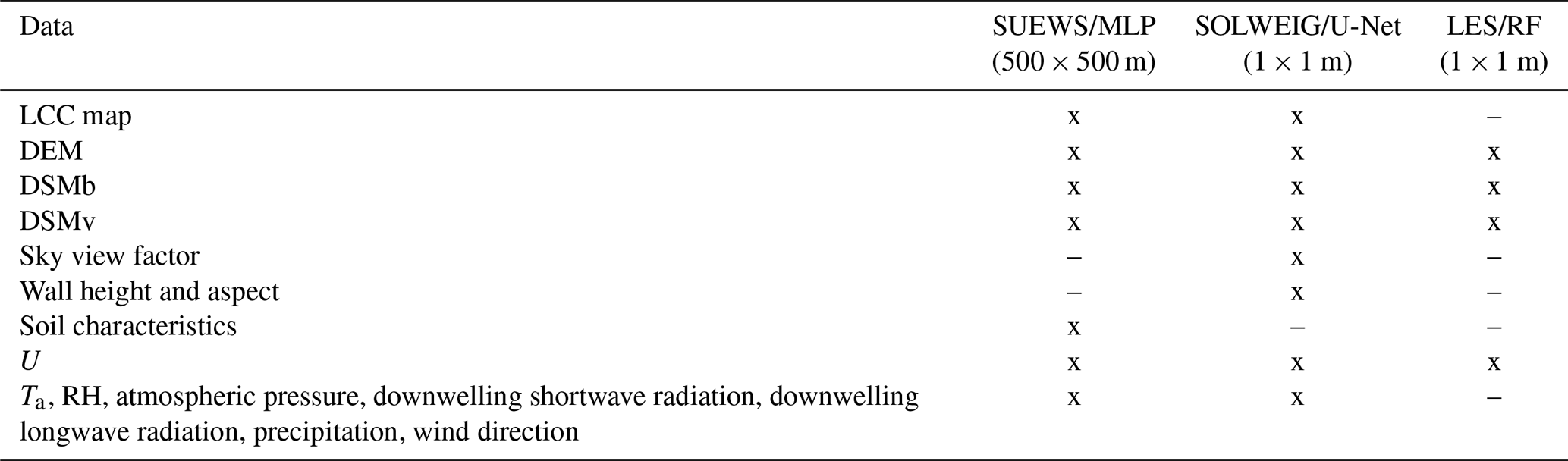
Spatial and forcing data are largely similar for the numerical models and their corresponding ML submodels; however, the MLPs use only a subset of all SUEWS input data (see Sect. 2.4), and the RF uses additional spatial predictors. The derivation of all spatial data other than anthropogenic dynamics is described in Briegel et al. (2023). A detailed overview of the spatial input and forcing data required for each submodel and their derivation is given in Table 2.

SUEWS does not require explicit building-resolved data but rather requires local-scale averaged spatial data. Information on urban morphology, land cover classes, and anthropogenic dynamics is required for SUEWS. Population density for each grid cell is derived from demographic data by city district (City of Freiburg im Breisgau – Bevölkerung, 2022). The remaining spatial input data, such as emissivity and albedo, are left at the default (Sun et al., 2021; Sun and Grimmond, 2019).

LESs and SOLWEIG require three-dimensional building geometry and tree characteristics derived from digital surface models (DSMs), digital elevation models (DEMs), and building outline data (Briegel et al., 2023), hereafter referred to as DSMb and DSMv.

Measurements from the urban weather station of the University of Freiburg are used as meteorological forcing data. The weather station is located on a rooftop (≈ 55 m a.g.l.; 48.0011° N, 7.8486° E) close to the city centre (Fig. 1). A detailed description of the urban weather station can be found in Briegel et al. (2023). The following variables are used as forcing data for SUEWS, the corresponding MLPs, and the U-Net: T_a, RH, atmospheric pressure, downwelling shortwave radiation, downwelling longwave radiation, precipitation, U, and wind direction. LESs and the RF model require only standard forcing related to an initial shear velocity of 1 m s⁻¹.

2.3 Validation data

Validation data for the MLPs and HTC-NN are derived from an urban weather sensor network in Freiburg (Fig. 1), which was installed in the summer of 2022. The sensor network covers the entire urbanized area and some rural areas, adjacent valleys, and hills to account for local weather phenomena such as mountain–valley wind systems or elevation effects which are not resolved by the ML model.

The stations of the sensor network can be divided into tier-I stations or biometeorological stations (7 stations) and tier-II stations (30 stations). Tier-I stations measure T_a, precipitation, RH, wind speed and direction, global radiation, and black-globe temperature (Feigel et al., 2023), while tier-II stations measure only T_a, precipitation, and RH (Plein et al., 2023). Tier-I stations are equipped with full weather sensors (ClimaVUE50, Campbell Scientific Inc., Logan, UT, USA) and black globe temperature sensors (model BLACKGLOBE-L, Campbell Scientific Inc., Logan, UT, USA). All sensors are mounted at 3.0 m a.g.l. on streetlights or custom poles, and the measuring interval is 1 min. Sensor network data in this study are aggregated to hourly values.

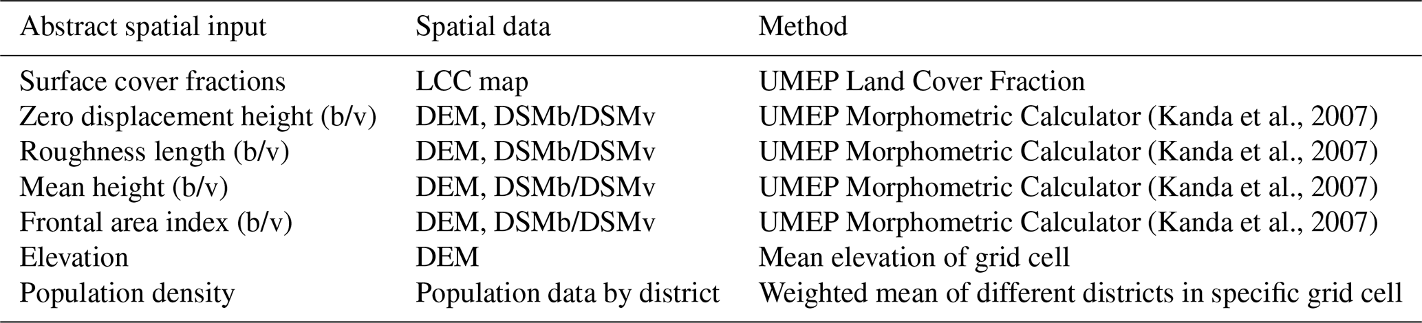
Table 1 Overview of the abstract input data, the spatial data, and the method used to derive the abstract input data. Most calculations are performed by the Urban Multi-scale Environmental Predictor (UMEP (Lindberg et al., 2018)). Spatial data contain land cover class (LCC), digital elevation model (DEM), and digital surface model (DSM). The suffix “b” indicates building data and the suffix “v” vegetation data.

Besides the sensor network, SOLWEIG is run for small subsets (50×50 m) around the tier-I stations to derive UTCI and T_mrt data for the specific locations of the tier-I stations (POI (point of interest) function; Lindberg and Grimmond, 2019). This allows a more detailed evaluation and a better attribution of the HTC-NN results.

2.4 Study period

The study period is aligned with the sensor network data which are collected from June 2022 onwards. The entire model period is from 2018 to 2022, with 2018 used as a spin-up year for SUEWS. The MLPs are trained with data from 2019 to 2021 and tested for 2022 (January–December). Model validation of SUEWS and the MLPs is performed with measurement data from June to December 2022, while the HTC-NN is validated with data from August to December 2022. During the entire model period, the mean annual T_a is 13.00 °C, the mean summer (June–August) T_a is 21.32 °C, and the mean maximum daily summer T_a is 26.27 °C. The number of hot days (maximum T_a≥30 °C) of the consecutive years from 2019 to 2022 is 26, 20, 9, and 37, respectively.

3 Modelling approach

The development of the HTC-NN requires four steps (Fig. 2). The first step is to generate initial spatial and meteorological data from various sources, which are listed in Table 2. In the second step, the so-called “ground truth” data (T_a, RH, T_mrt, and U) for the four HTC-NN submodels (two MLPs, U-Net, and RF) are calculated using numerical models (SUEWS, SOLWEIG, and LES). Training and evaluation of the HTC-NN submodels are done in the third step, while the fourth step is to link these submodels by calculating UTCI. As the U-Net has already been trained and validated, only the development and the requirements of the MLPs and the RF (spatial and temporal data, SUEWS, and LES) are explained.

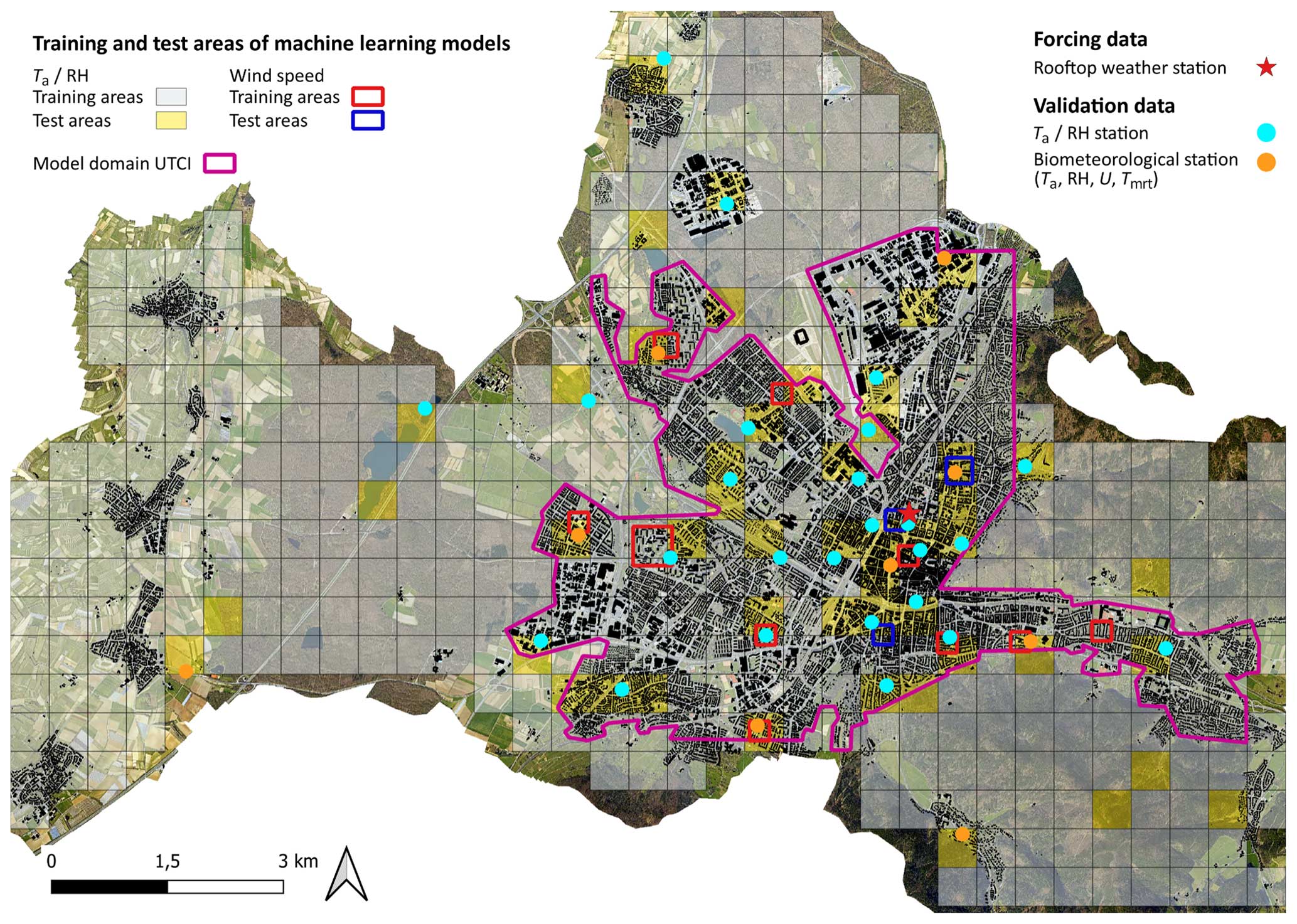
Figure 1 Model domain of the city of Freiburg, Germany. The red star shows the location of the rooftop weather station used for forcing data. Orange and turquoise points show the locations of the urban sensor network used for model evaluation. Grey grid cells show the training areas of the T_a and RH submodels, while yellow grids show the test areas. Red and blue squares show the training and test areas of the U submodel, respectively. The pink border shows the prediction area of UTCI. Orthophoto in the background based on data from the City of Freiburg, http://www.freiburg.de (last access: 4 May 2021).

3.1 Numerical modelling

3.1.1 Local-scale T_a and RH modelling (SUEWS)

SUEWS (version 2020a) is used to model T_a and RH at 2.0 m a.g.l. for 436 grid cells with a resolution of 500 × 500 m (Järvi et al., 2011; Ward et al., 2016). SUEWS has been validated in different cities under different climatic conditions (Ao et al., 2018; Järvi et al., 2011; Ward et al., 2016). Besides the following parameters, SUEWS is run in default mode: net radiation method, maximum and minimum porosity, and roughness length of the momentum method. The net radiation method is set to 1 as downwelling longwave radiation data are available. The maximum and minimum porosities of deciduous trees are set to 0.6 and 0.2, respectively (Ward et al., 2013). Roughness length and zero displacement height are calculated according to Kanda et al. (2007) and are provided to SUEWS, so the roughness length method is set to 1. As mentioned, SUEWS is run for 2018–2022, while 2018 is excluded from subsequent modelling as it serves as a spin-up year.

Table 2 Overview of required spatial and forcing data for the numerical and machine learning models. Note that SUEWS and MLP use abstract spatial data (see Table 1), and the RF model uses additional spatial predictors derived from DEM, DSMb, and DSMv which are not listed here.

3.1.2 Micro-scale U modelling (LES)

LESs are used to obtain micro-scale (1 × 1 m) wind fields for 12 areas ranging in size from 122 × 122 to 500 × 500 m. The LES model code and set-up are described in Giometto et al. (2016) and (2017). LES needs DSMb and DSMv as spatial input data. Training and test areas are carefully selected to ensure that the variability of the urban environment is adequately represented. For each area, four LESs are computed for pressure gradients that cause northward, eastward, southward, and westward inflow directions. The simulations are set up with an identical standard forcing related to an initial shear velocity of 1 m s⁻¹. Each simulation contains 30 min (steady-state) wind field data in 2 s steps, which are then time averaged.

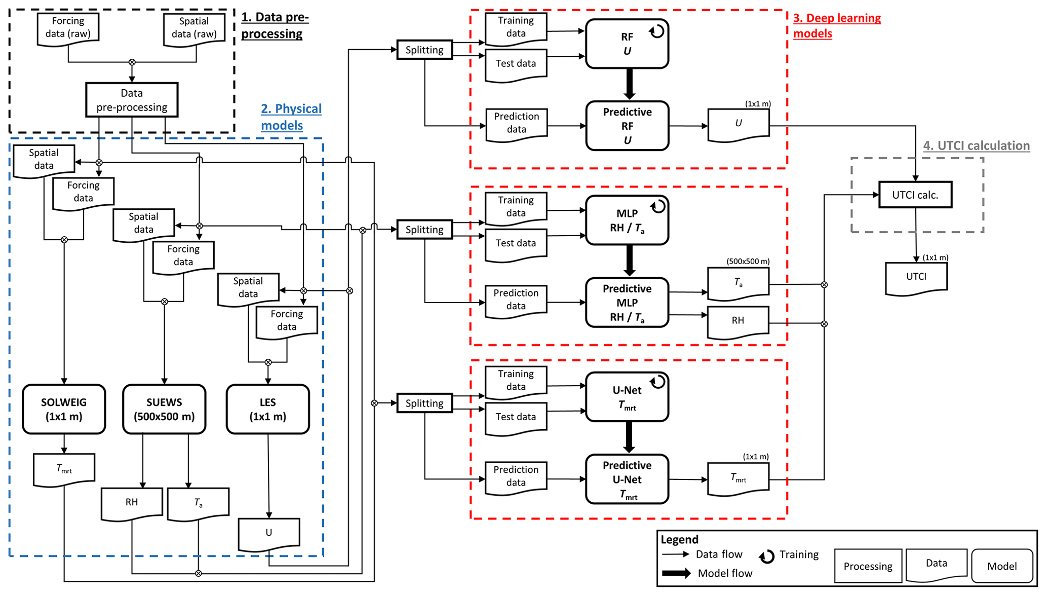
Figure 2 Workflow of the HTC-NN model development: (1) data pre-processing, (2) numerical modelling of ground truth, (3) training and evaluation of machine learning models, and (4) calculation of UTCI.

3.2 Machine learning models

3.2.1 Multi-layer perceptron model development

The MLPs are designed using Python and the PyTorch library. To determine the best model architecture, a model-based Bayesian hyperparameter optimization is performed. For this purpose, the Optuna software framework (Akiba et al., 2019) is used in combination with PyTorch. Training and prediction are conducted on an NVIDIA GeForce RTX 3080.

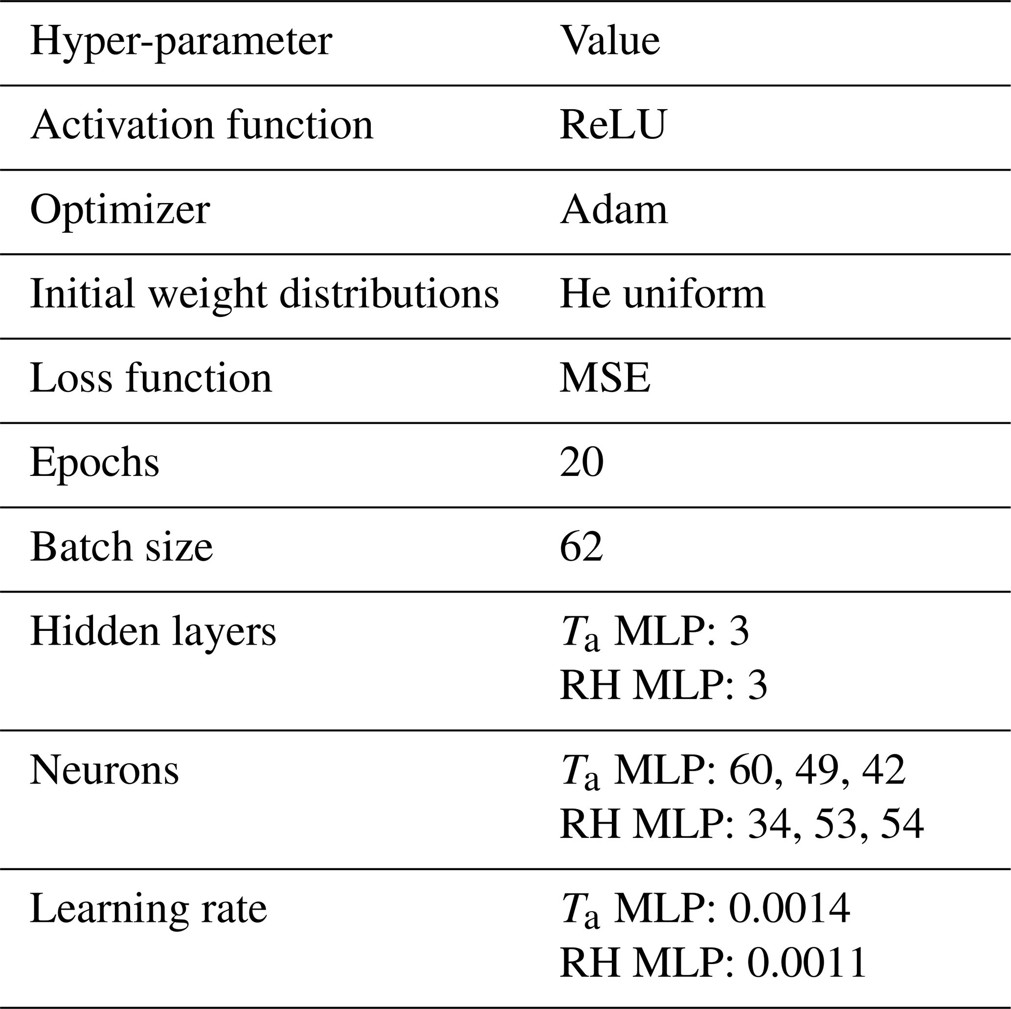
T_a and RH are each modelled with their own deep learning model. Differently to the T_mrt deep learning model, which is based on a convolutional neural network, T_a and RH models are built from fully connected feed-forward artificial neural networks known as MLPs. This is because the different SUEWS grid cells are not connected and have no spatial relationship. MLPs consist of three different types of layers: an input layer, hidden layer, and an output layer. Bayesian optimization determines the number of hidden layers and neurons, the presence or absence of a dropout layer, and the learning rate that leads to the highest model accuracy. In total, 30 hyperparameter combinations (trials) are tested for each model. For this purpose, the training dataset is further divided into training and evaluation datasets, and a 3-fold cross-validation is used to validate each hyperparameter trial. The hyperparameter combination of each trial is defined by the Tree-structured Parzen Estimator (TPE) (Bergstra et al., 2011, 2013), which is a Bayesian hyperparameter optimization algorithm. The best architectures of both MLPs have three hidden layers with 60, 49, and 42 neurons for the T_a MLP and 34, 53, and 54 neurons for the RH MLP. Learning rates are best at 0.0014 and 0.0011 for the T_a MLP and RH MLP, respectively. Drop-out layers do not improve the model accuracy and are not added to the final models. The remaining hyperparameters, such as activation function, optimizer, and initial weight distribution, are taken from the literature (Table 3 and Briegel et al., 2020). As an evaluation metric (loss function), mean squared error (MSE) is used. For further comparisons, root mean square error (RMSE) and mean bias error (MBE) are used.

3.2.2 Random forest model development (U)

The RF modelling is conducted in MATLAB (The Mathworks, Natick, MA, USA, version 2021b) using a regression-bagging approach with 50 learning cycles. In addition to spatial building and tree data, spatial features (derived from DSMb) are predictors. These predictors are indices pertaining to the street length and width, frontal area index relative to the flow direction, horizontal Euclidean distance, and up- and downwind distances to buildings. For each of the 12 training areas and the three components of the wind field, individual models are trained (u: streamwise, v: normal-to-streamwise horizontal, w: vertical), resulting in 36 models. This model ensemble makes predictions for each component, which are then assembled as the Euclidean norm of u, v, and w to obtain the final wind field. The RF models can theoretically compute wind fields for any wind direction over the city, requiring only an adjustment of the predictors. However, for the purpose of calculating outdoor thermal comfort, citywide wind fields are computed only for the northward (315–45°), eastward (45–135°), southward (135–225°), and westward (225–315°) inflow directions, each covering a 90° angle. The LES wind fields are scale-independent, allowing a linear rescaling of the RF model output. Thus, a time series of city-wide wind fields can be computed by hourly wind speed data from the urban weather station.

Table 3 Hyper-parameters of both MLP models.

3.3 Thermal indices

In the final model step, the results of the above-mentioned submodels are combined into a thermal comfort index with a spatial resolution of 1 × 1 m. However, not all indices are appropriate for human thermal comfort (Staiger et al., 2019). Therefore, only UTCI (Błażejczyk et al., 2013), which is widely used in urban climate science and planning, is considered in this study. The reference conditions of UTCI correspond to an individual walking outdoors with T_mrt equal to T_a, no wind, and RH at 50 %. The UTCI values can be categorized based on thermal stress; e.g. UTCI values ranging from 32 to 36 °C are assigned to strong heat stress. The different UTCI stress categories and the corresponding UTCI ranges are listed in Table A1 in the Appendix.

4 Results

This section presents the evaluation of the three submodels of the HTC-NN (Sect. 4.1), the HTC-NN itself (Sect. 4.2), and the high-resolution UTCI mapping of the HTC-NN (Sect. 4.3).

4.1 Evaluation of T_a, RH, and U submodels

The accuracies of SUEWS, SOLWEIG, the MLPs, U-Net, and RF relative to the sensor network are shown in Fig. 3 and Table 4. A spatial evaluation of machine learning models in relation to numerical models in their specific test areas is given in Table B1.

With RMSEs of 1.50 and 1.51 K, respectively, the SUEWS and T_a MLP models demonstrate similar performances compared to the sensor network data. Both models' RMSEs are about 0.30 K lower than the forcing data. The errors of SUEWS and the MLPs across the different stations are similar (Fig. 3a), with a higher variability during the night than during the day. Figure 4b shows a moving average of RMSE over time for the final HTC-NN model and for the T_a and RH MLPs (Fig. 4c and d). It can be seen that the RMSE of the T_a MLP shows two peaks in late October and mid-December, while the RMSE fluctuates around 1.00 K during the remaining time. Overall, the T_a MLP shows good accuracy compared to the SUEWS model (R² of 0.997 and RMSE of 0.50 K). Similar observations can be made for the RH MLP. RMSEs for SUEWS and the MLP model are 7.79 % and 8.14 %, respectively, while the RMSE of the forcing data is 9.08 %. Similarly to the T_a models, the RMSE of the RH MLP has two strong peaks in late October and mid-December, with RMSE values up to 15 %, while RMSE fluctuates around 5 % to 6 % during the remaining time. R² values of SUEWS and the RH MLP are lower at 0.88 and 0.87 compared to 0.97 for the T_a models. Nevertheless, the overall R² between SUEWS and the RH MLP is high at 0.98, and with an overall RMSE of 3.28 %, the accuracy of the RH MLP is considered to be satisfactory. The T_mrt U-Net has a slightly lower accuracy than SOLWEIG (RMSE of 6.18 to 5.86 K; R² of 0.84 to 0.86). A detailed evaluation can be found in Briegel et al. (2023). The RF has an R² of 0.28 and an RMSE of 0.74 m s⁻¹ in relation to sensor network data and shows a large improvement compared to forcing data (RMSE of 2.85 m s⁻¹). However, the R² of RF U is lower than the R² of forcing data. The RF model has an overall accuracy of 0.76 m s⁻¹ (RMSE) compared to the LES model (Table B1).

Table 4 MAE, MBE, RMSE, and coefficient of determination (R²) of numerical and machine learning models and sensor network data for T_a, RH, U, T_mrt, and UTCI. Additionally, errors between forcing data and sensor network data are added for T_a, RH, and U (as baseline). Note that T_a and RH are validated on tier-I and tier-II stations, while U, T_mrt, and UTCI are only validated on tier-I stations.

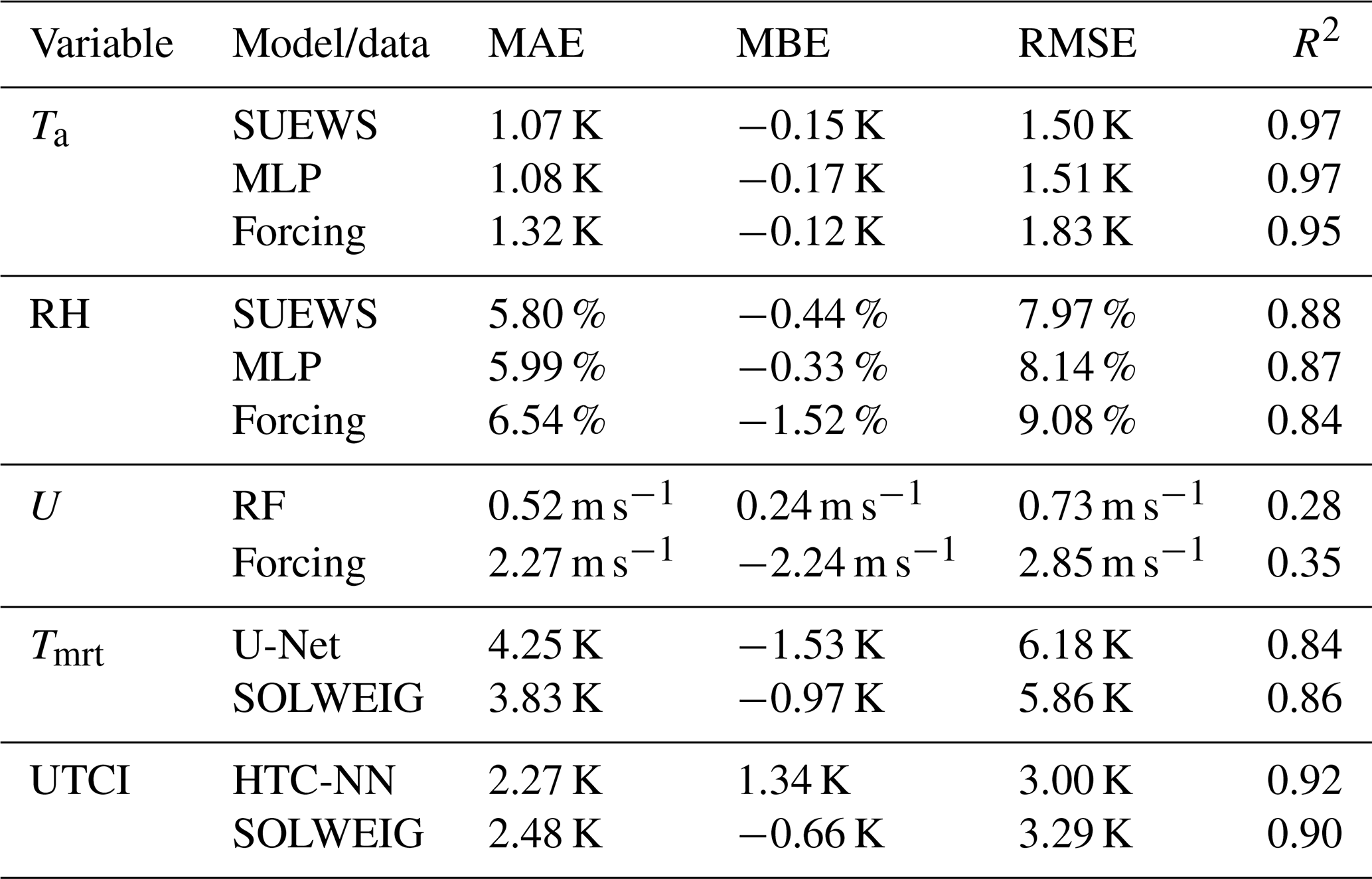
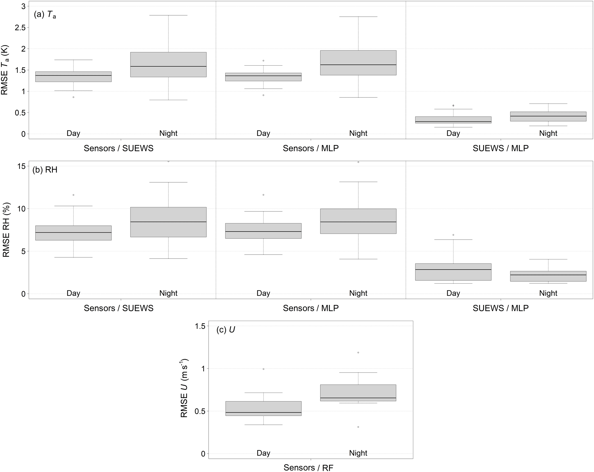
Figure 3 Box plots of RMSEs of SUEWS and MLPs compared to sensor network data and between SUEWS and the MLPs for T_a (a) and RH (b), respectively, and their differences between day and night. In (c) the RMSE of U between sensor network data and RF is shown. Box plots show dispersion of different sensor network stations.

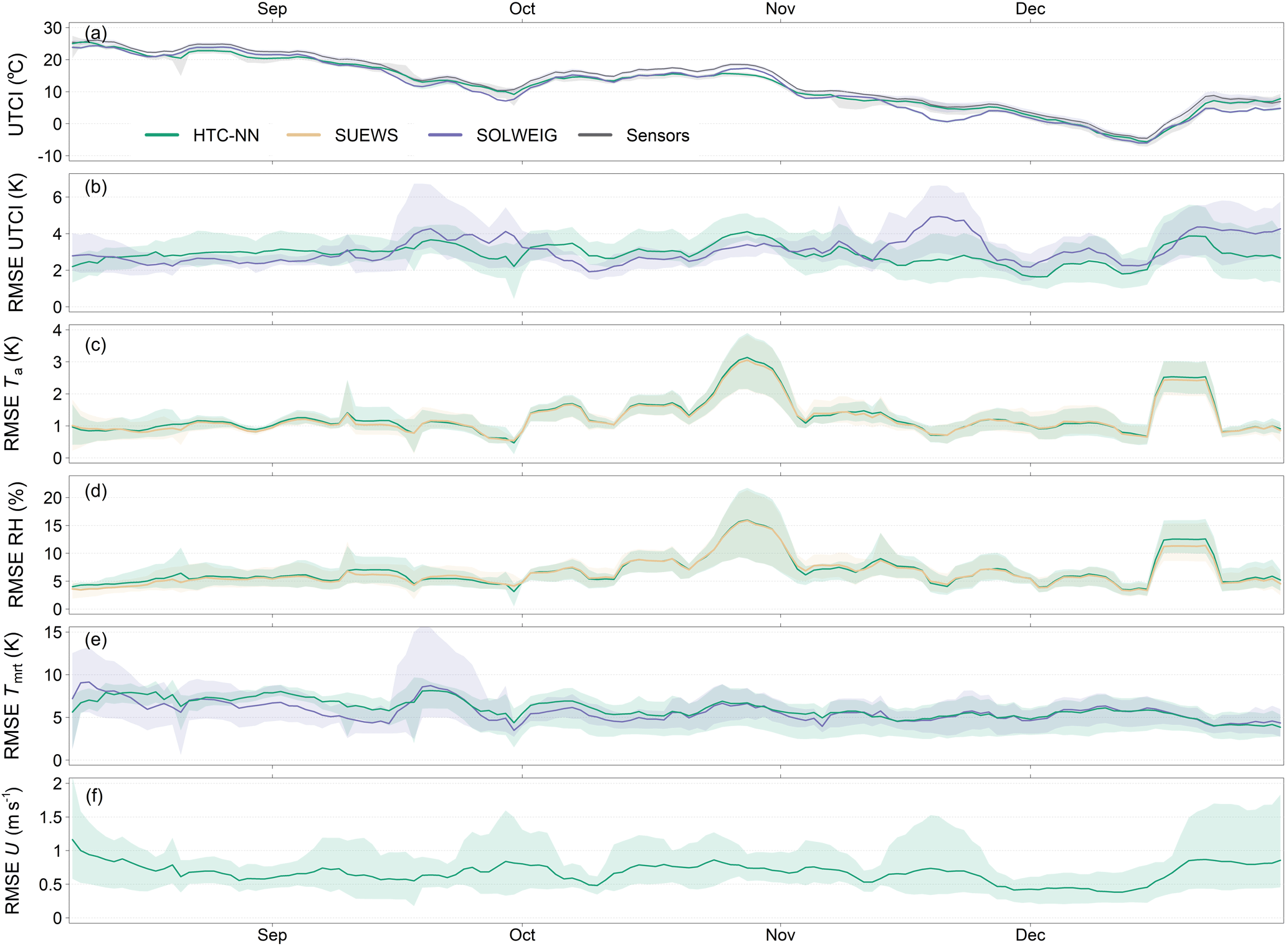
Figure 4 Moving average of UTCI (a) and RMSE of UTCI (b), T_a (c), RH (d), T_mrt (e), and U (f) from August to December 2022. The window size of the moving average is 7 d. Time series starts with the installation of the first tier-I stations in August 2022. In (c) and (d) RMSEs of SUEWS predictions are added for comparison (orange lines). In (b) and (e) RMSEs of SOLWEIG predictions are added (violet lines). For U, no numerical model results exist. Shaded areas represent 95 % confidence interval.

4.2 HTC-NN evaluation

The HTC-NN has an RMSE of about 3.00 K and an R² of 0.92 (in relation to the sensor network), while SOLWEIG has an RMSE of 3.29 K and R² of 0.90 (Table 4). Moving averages of UTCI and RMSE (window size of 7 d) over time (August–December 2022) and diurnal error patterns are shown in Figs. 4 and 5. The annual RMSE of UTCI ranges between 2 and 4 K, with the highest RMSE values in mid-September, late October, and mid-December. T_a and RH show a similar pattern in October and December, while T_mrt has its largest errors in August and September, ranging from 6 to 8 K. The RMSE of U varies between 0.5 and 1 m s⁻¹, with the highest values in August, late October, and late December. The elevated RMSE values of UTCI in mid-September coincide with the RMSE peak of T_mrt in mid-September, while the RMSE peaks for UTCI in late October and December match the high RMSE values for T_a and RH in those periods. In Fig. 4b and e, results from SOLWEIG are added (violet lines). SOLWEIG is more accurate than the HTC-NN in modelling UTCI and T_mrt in summer, while the HTC-NN is more accurate in autumn and winter. Diurnal patterns of UTCI accuracy are shown in Fig. 5a. Model errors are lower during the night than during the day, with the highest errors during the morning. The U-Net T_mrt error is also lowest during the night but has its highest errors in early evening (see also Briegel et al., 2023). The T_a and RH MLPs have similar error patterns and are lowest in the late afternoon. The diurnal pattern of the U RF model accuracy shows higher accuracy during the day than at night.

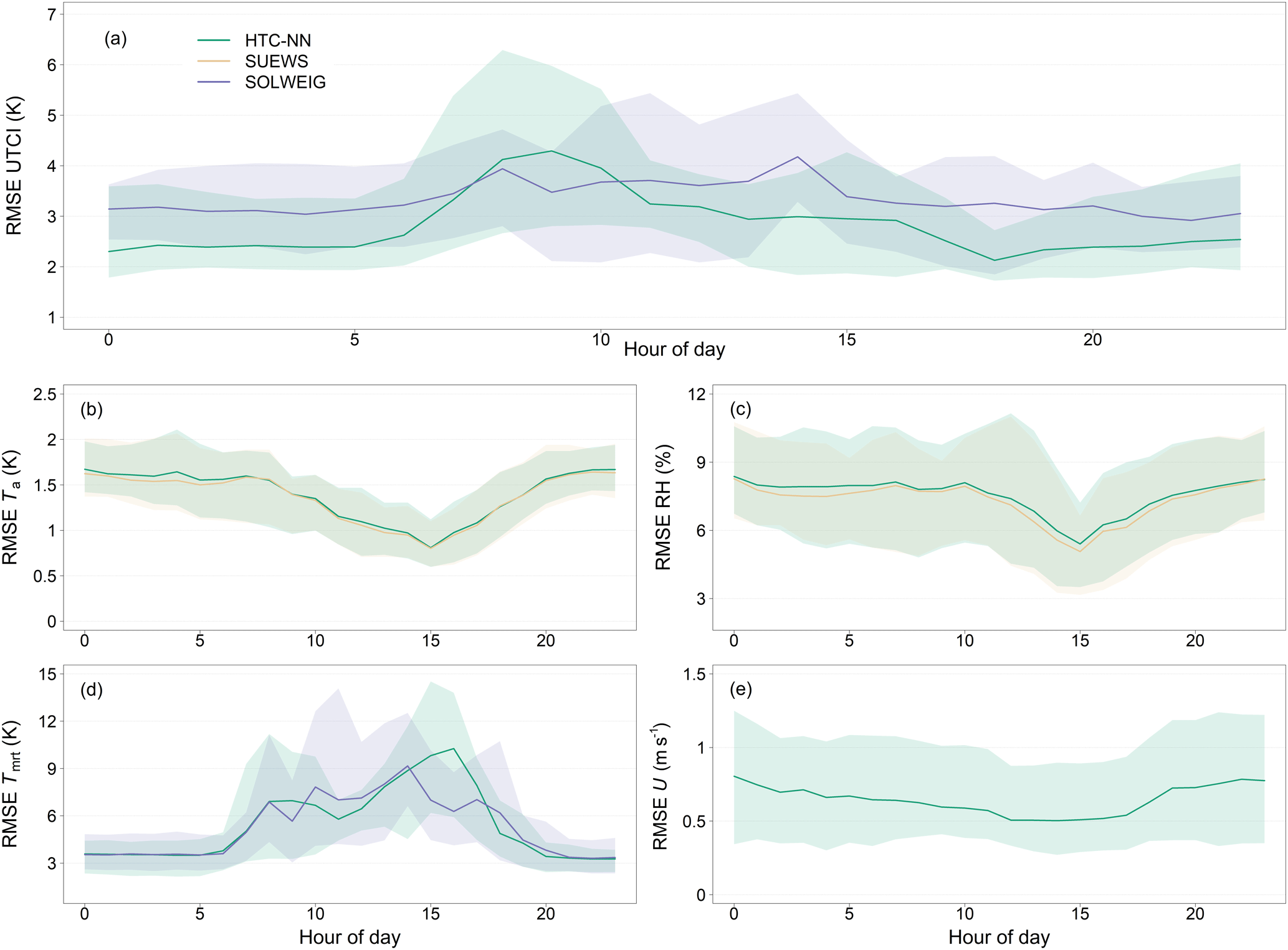
Figure 5 Normalized diurnal RMSE of UTCI (a), T_a (b), RH (c), T_mrt (d), and U (e). In (b) and (c) RMSEs of SUEWS predictions are added for comparison (orange lines). In (a) and (d) RMSEs of SOLWEIG predictions are added (violet lines). For U, no numerical model results exist. Shaded areas represent 95 % confidence interval.

Figure 6 shows sensor network and modelled UTCI values (HTC-NN and SOLWEIG) at five stations during an exemplary heatwave event in August 2022. Daytime UTCI is overestimated by the HTC-NN to varying degrees (between 1 and 5 K), while nighttime predictions are in line with measurements. In Fig. 6c, the HTC-NN underestimated UTCI in the afternoon, which is in line with underestimated T_mrt. SOLWEIG, on the contrary, underestimates UTCI in the morning and overestimates it in the afternoon and evening. Figure 6e shows significantly lower UTCI and T_mrt values for SOLWEIG during the afternoon, while the HTC-NN does not show this pattern.

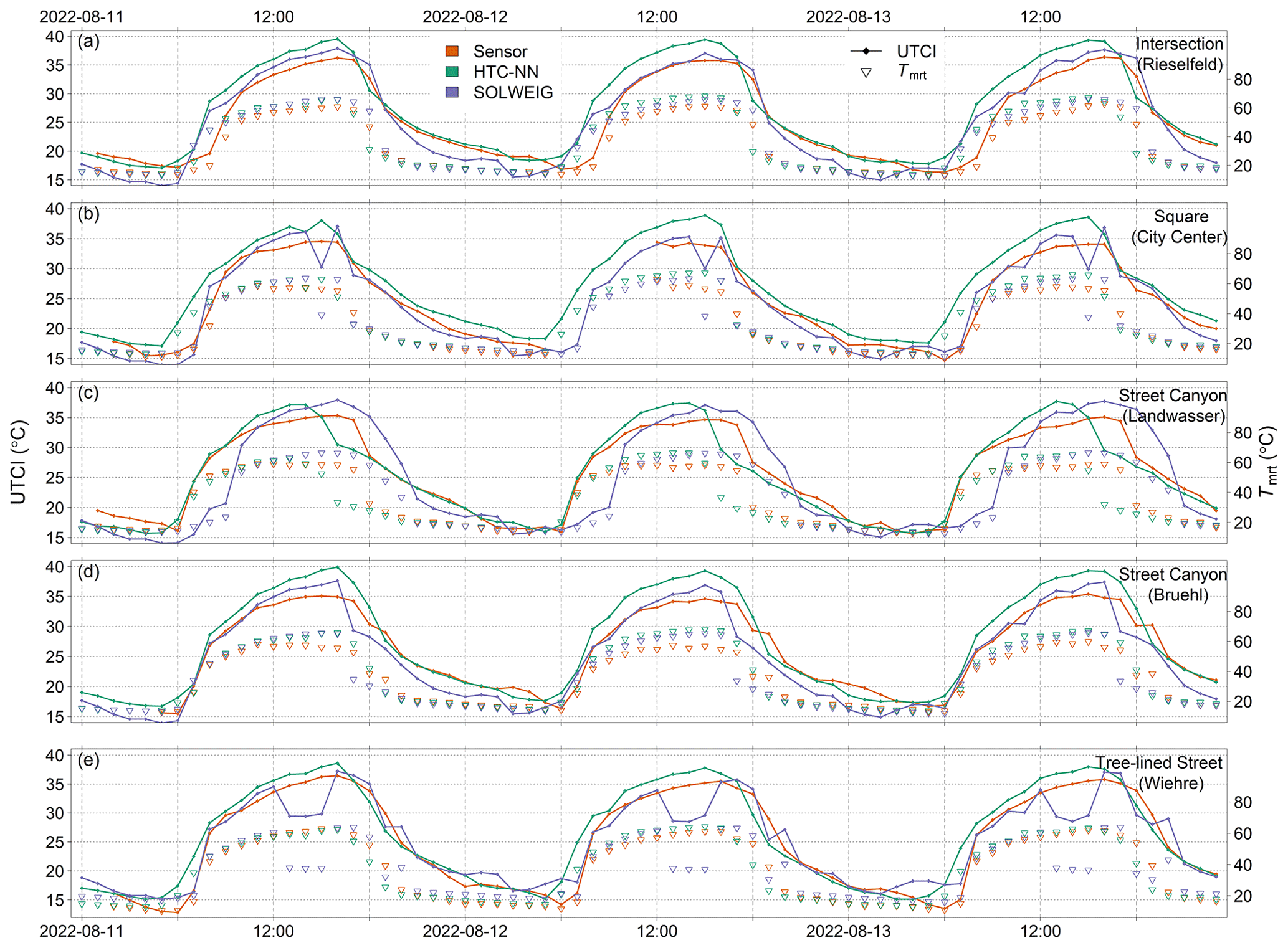
Figure 6 Modelled and measured UTCI and T_mrt at five tier-I stations (a–e) during a heatwave event in August 2022.

In Fig. 7, distributions of both sensors and models and their differences are shown. The HTC-NN has a higher share of values between 15 and 25 °C, whereas shares of UTCI greater than 25 °C are equal. SOLWEIG, on the contrary, has lower shares for almost all the bins below 2.5 °C and higher shares between 5 and 12.5 °C.

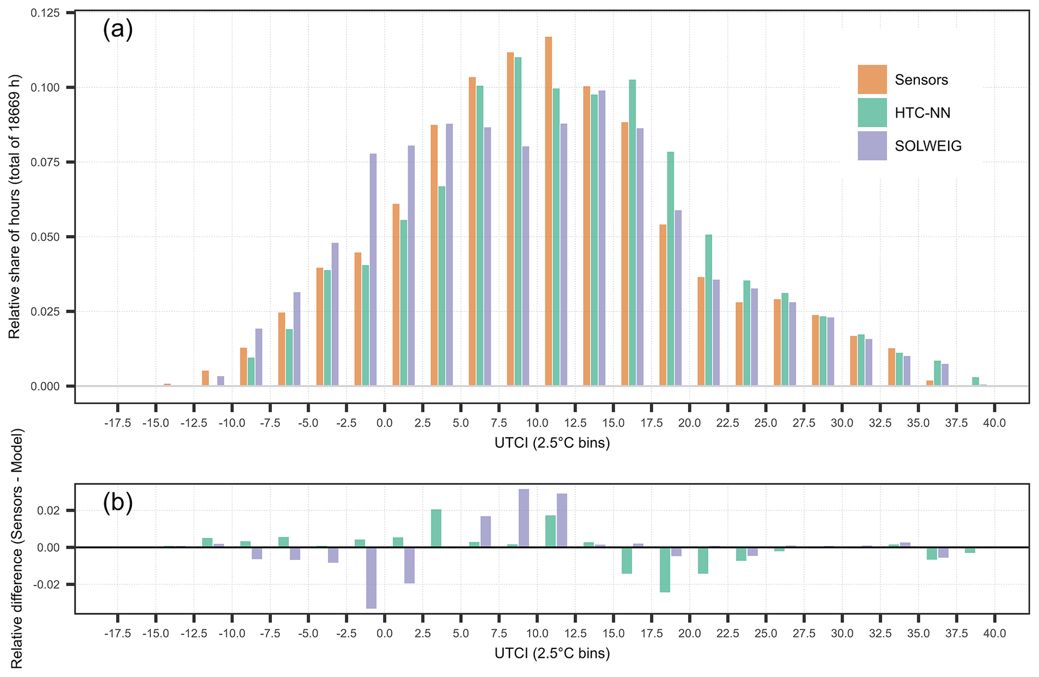
Figure 7 UTCI distributions from sensors, HTC-NN, and SOLWEIG (a) and the differences between models and sensor network (b). Distributions are shown for bins with a size of 2.5 °C, along with their relative share in total hours (n=18 669 h).

4.3 High-resolution UTCI mapping

This section presents an application of the developed HTC-NN for mapping and downscaling the simulated UTCI at 1 m resolution for Freiburg. Calculating hourly UTCI over 4 years (35 064 time steps) and 42.5 million pixels using an Intel Core i9 processor and NVIDIA GeForce RTX 3080 took only about 8 d. No individual runs are saved as this would exceed storage capacities, and predictions are stored as day- and nighttime sums of hours for each month within 1 °C UTCI bins.

Figure 8 shows the spatial distribution of cumulative daytime hours with strong, very strong, or extreme heat stress. This figure shows heat hotspots related to daytime heat stress as UTCI values ≥ 32 °C are rarely reached at night without solar radiation (Fig. 11b). Figure 10 shows the same map extent but with nighttime hours exceeding a UTCI value of 22 °C. Figures 9 and B3 provide a more detailed view of four exemplary urban areas representing the LCZs 2, 5, and 8. These areas show not only the thermal comfort difference between different LCZs but also the intra-LCZ variability (Fig. 9c and d).

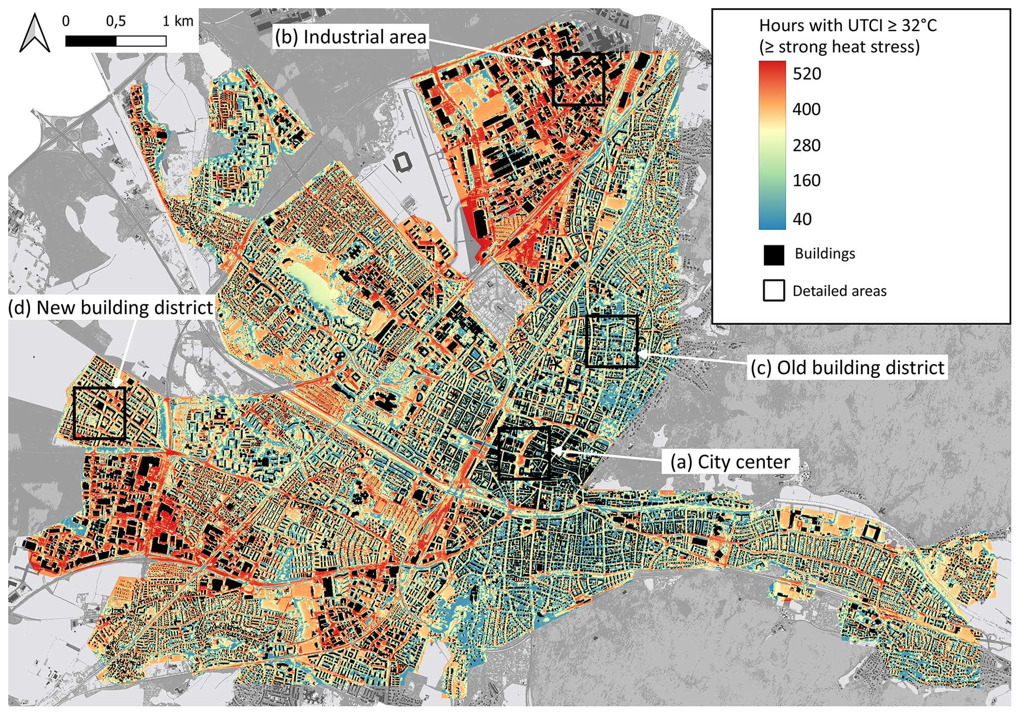
Figure 8 Map of Freiburg representing the average number of daytime hours with a UTCI ≥ 32 °C per pixel (corresponds to strong and more heat stress). Note, colouring is in accordance with predicted UTCI quantiles. The spatial resolution of the map is 1 × 1 m, and the time period for averages is 2019–2022. Rectangles (a–d) define areas shown in more detail in Figs. 9, 11, and B3.

The four areas represent the densely built-up city centre with parts containing large trees but also large open and paved areas (a), an industrial area with mostly paved surfaces and only a few trees (b), an old building district with a large and old tree stock (c), and a relatively new district built in the period 1995–2005 (d).

In Fig. 9, it is quickly apparent that there are large differences due to shading and tree canopy cover during the day and night. Figures 9e and B3e show the distributions of the spatially distributed numbers of hours in Fig. 9a–d. The distributions confirm the visual perspective. The industrial area (b) and the new building district (d) have a higher share of pixels, with more hours exceeding the threshold of 32 °C during the day and fewer hours exceeding the threshold of 22 °C during the night. In turn, the densely built-up city centre (a) and the old building district (c) have fewer hours ≥ 32 °C but more hours ≥ 22 °C. Figure 11 shows the summertime UTCI distributions during the day- and nighttime for these four areas. The distributions underline the visual assumption that tree-covered and less-paved areas are less affected by thermal stress during the daytime but have higher UTCI values during the nighttime. In addition, Fig. 11 shows the 80th percentiles of the different areas, ranging from 29 °C (old building district) to 32 °C (industrial area) during the daytime and from 21 to 22 °C during nighttime. The 80th percentiles highlight the importance of shading to daytime outdoor thermal comfort. During the nighttime, however, the industrial area and the new building district cool down more quickly, resulting in lower UTCI values and 80th percentiles (21 °C vs. 22 °C). Although there is a cooling effect at night, the shading effect during the day is stronger than the reduction in nighttime cooling. These results indicate that outdoor thermal comfort controls have an inverted effect during the day and the night.

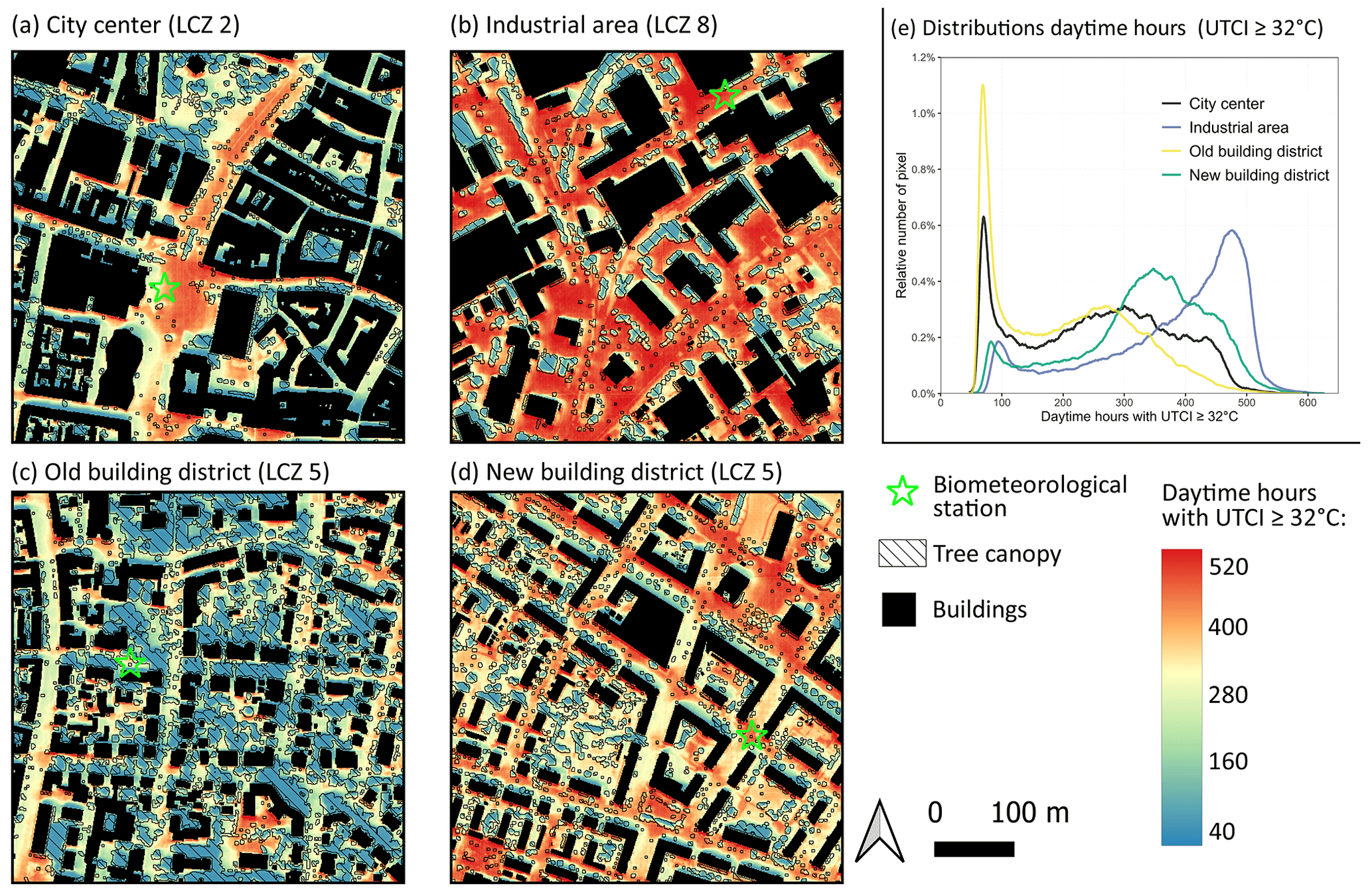
Figure 9 Four 500 × 500 m subsets of different urban neighbourhoods of Freiburg. Average hours per year with a UTCI ≥ 32 °C are shown. Panel (a) shows the city centre of Freiburg, panel (b) shows an industrial area in the north of Freiburg, panel (c) shows a district with old buildings and dense or mature tree stock, and panel (d) shows a building district built after the year 1995. Panel (e) shows the distributions of (a)–(e). Note, colouring is in accordance with predicted UTCI quantiles. The spatial resolution is 1 × 1 m, and the time period is 2019–2022.

There are differences not only between the different LCZs but also within the same LCZ class. The old building and the new building districts show strong differences in their day- and nighttime UTCI distributions. The difference between those two areas is larger than between the city centre and the old building district or between the industrial and new building districts. The areas do not differ much in their physical building characteristics and are both classified as LCZ 5. However, the old building district has a tree cover fraction of 45 % and can be further defined as LCZ subclass 5_b, while the new building district has only 24 % tree cover and can therefore defined as LCZ 5_d.

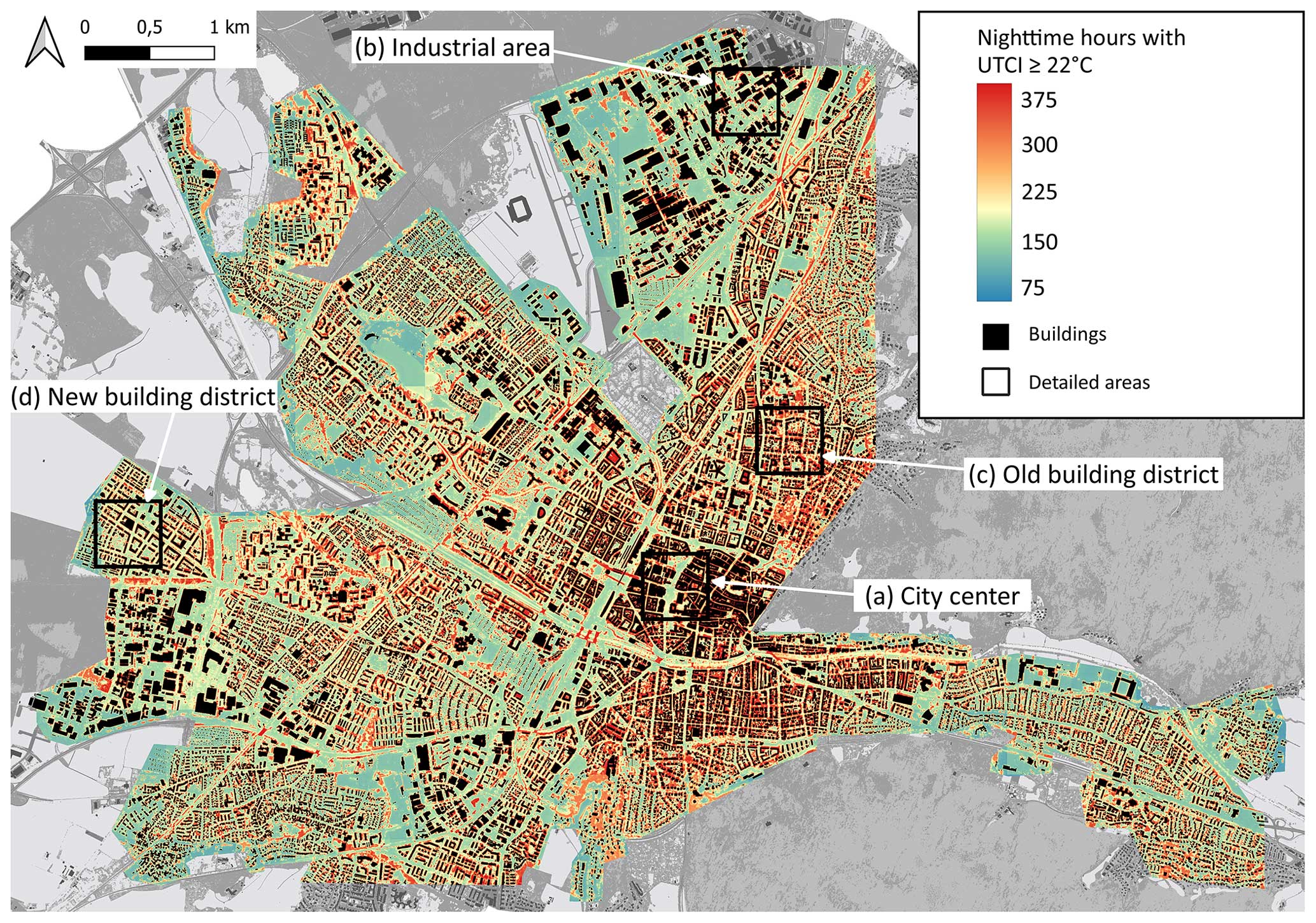
Figure 10 Map of Freiburg representing the average number of nighttime hours with a UTCI ≥ 22 °C per pixel. Note, colouring is in accordance with predicted UTCI quantiles. The spatial resolution is 1 × 1 m, and the time period is 2019–2022. Rectangles (a–d) define areas shown in more detailed in Figs. 9, 11, and B3.

In Fig. 10, sharp UTCI transitions are partially visible. These transitions occur between adjacent grid cells (500 × 500 m) of the T_a and RH MLPs (original SUEWS grid cells). The transitions are more prominent in Fig. 10 than in Fig. 8 as T_mrt influences diurnal UTCI more than T_a. The transitions between grid cells also illustrate that T_a and RH are modelled individually for each grid cell without interaction with adjacent cells.

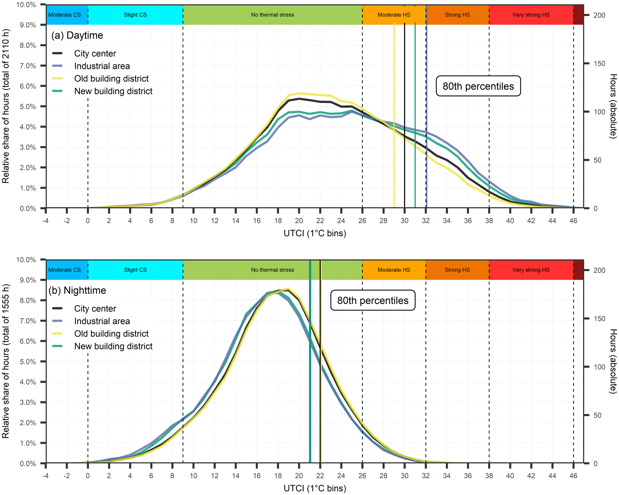
Figure 11 Summertime (May–September) distributions of UTCI of the four districts shown in Figs. 9 and B3 during the daytime (a) and during the nighttime (b). On top of each figure the UTCI heat stress classes are presented (CS: cold stress; HS: heat stress). Vertical lines in the colours of the four areas represent the 80th percentiles. The left y axis shows the relative number of hours, and the right y axis shows the absolute number of hours. Note that the x axis has a bin size of 1 °C; the total number of hours varies between (a) and (b) because of the day length in summer.

5 Discussion

5.1 Evaluation of the HTC-NN submodels

Both MLPs show promising results compared to measurements and especially compared to the numerical model SUEWS. With an overall (spatial) R² of 0.997 and an RMSE of 0.5 K, the T_a MLP shows excellent accuracy. Both SUEWS and the T_a MLP have an RMSE of around 1.5 K in relation to sensor network data, while the MAE is only around 1 K. RMSE also varies with time (Fig. 4c). Apart from the two periods of late October and mid-December, with RMSE values higher than 2 K, the RMSE fluctuates around 1 K for most of the remaining time. This suggests that the overall RMSE of 1.5 K is highly influenced by the two outlier periods in late October and mid-December, with high RMSE values between 2 and 3 K. For the RH MLP, similar observations are made, having higher RMSEs in late October and mid-December. Since the MLPs and the SUEWS model have similar error patterns, the error must already be apparent in forcing data (see also Fig. B1). The end of October was unusually warm, with clear sunny days but cold nights. As forcing data are measured on a rooftop at 55 m a.g.l., the near-surface night cooling is not represented in these data, leading to higher RMSE values. In December, on the other hand, an uncommon weather event occurred with a surface inversion between the surface and the rooftop at 55 m a.g.l., with colder air near the surface and warmer air above. Compared to the ERA5-Land data, the forcing and model data show higher errors during these periods in October and December, indicating that errors are already present in the forcing data and are passed on to the model results. Both SUEWS and the MLP have a lower RMSE than the forcing data in relation to the sensor network data. However, the gain in accuracy is moderate for RH at 1 % and for T_a at 0.3 K. One reason could be that SUEWS is set up in default mode, and no specific model calibrations are performed. In addition, the modelled soil moisture has not been validated against measurement data. Another reason could be that SUEWS is run in offline mode. Running SUEWS in online mode, coupled to a mesoscale weather model, would probably increase its accuracy further as boundary conditions and tile interactions, including local wind systems, would be better mapped.

The RF approach to modelling a statistical wind field for the entire urbanized area of Freiburg shows good results for outdoor thermal comfort modelling. Since the RF models a statistical wind field only, not every wind gust can be accurately represented. Still, as the model is forced with hourly aggregated data, it is sufficient to predict hourly averaged U.

The results of the evaluation of the T_a and RH MLPs and the RF illustrate the power and potential of deep and machine learning models in the context of urban climate when appropriate training data are available. It can also be seen that the MLPs have similar model shortcomings to SUEWS, and an enhanced MLP performance requires an improved numerical model.

5.2 Evaluation of HTC-NN

The trade-off between the computational cost and model accuracy of the HTC-NN compared to numerical models is positive for both. The HTC-NN has a higher model accuracy than SOLWEIG with its POI option. In addition, model accuracy is constant throughout the year, with lower accuracy during less common weather conditions. As mentioned, uncommon weather situations with strong surface inversions in the city are hard to predict for numerical and deep learning models. The overall RMSE of UTCI is around 3 K. The lower RMSE of the HTC-NN compared to SOLWEIG can be explained by the combination of four submodels that downscale T_a, RH, T_mrt, and U separately, while SOLWEIG downscales only T_mrt comprehensively. Diurnal error patterns of UTCI show higher errors during the day than during the night due to higher errors in the T_mrt predictions. However, the highest errors occur before noon, while in the late afternoon, when thermal stress is highest, UTCI predictions are more accurate (RMSE of about 3 K). During the heatwave event, the HTC-NN overestimates UTCI to different degrees during the day. It is also apparent that daytime UTCI follows the patterns of T_mrt most of the time, emphasizing the importance of correct shadow pattern data. Since T_mrt predictions of SOLWEIG and HTC-NN are partly in line while UTCI values differ, the prediction error must be related not only to T_mrt but also to T_a and RH, while U is negligible on these days. These results indicate that the accuracy of the HTC-NN is affected to varying degrees by its submodels under different weather conditions and that an overall attribution of error to the submodels cannot be made but must be done individually for the different weather conditions.

To the authors' knowledge, not many comparisons (of at least 1 week) have been made between UTCI models and measurements. Nice et al. (2018) used a modified version of the TUF-3D model (Krayenhoff and Voogt, 2007) to model UTCI in a suburb of Melbourne for 4 weeks. Observed UTCI values were calculated from T_mrt (black globe), T_a, RH, and U measurements. A total of seven stations were installed and compared to model results. The MAE between modelled and observed UTCI ranged from 1.80 to 3.03 K, and the RMSE ranged from 2.33 to 3.64 K, which aligns with HTC-NN. On the other hand, Meili et al. (2021) applied the ecohydrological model UT&C in Singapore with the model accuracy for UTCI ranging from 1.9 to 3.1 K (RMSE). Since Freiburg is hardly comparable to Melbourne or Singapore, these findings still help to better evaluate the HTC-NN model results. The HTC-NN has a similar accuracy but allows for modelling larger domains at a high resolution.

While the HTC-NN has a very good trade-off between accuracy and computational cost, it has some limitations. First, the HTC-NN is not coupled to a mesoscale model and thus does not include local or mesoscale weather phenomena, such as mountain–valley wind systems, cold-air drainage, and advection of heat (e.g. heat island and urban plume). Additionally, while large model domains are possible, the 500 × 500 m model tiles for T_a and RH are modelled individually, and no boundary or heat and moisture transport effects are considered, similarly to the offline SUEWS version. These constraints are related to the model structure of the offline SUEWS version and could be partially resolved by running it coupled to a mesoscale model. Another constraint is related to the forcing data. The HTC-NN is forced with meteorological data from a weather station at 55 m a.g.l. Measured T_a at this height may already be exposed to other processes such as near-ground-level T_a, which may lead to initial error propagation. Additionally, the larger the model domain, the more difficult it is to force the model with data from one weather station. This could be solved by forcing the HTC-NN with reanalysis data or weather forecast products, which would reduce the model fit due to inconsistencies between measured and reanalysis and forecast data. As the submodels perform well in emulating the numerical models, better numerical models would also be needed to increase the accuracy of the model itself (Briegel et al., 2023). Nevertheless, the HTC-NN should only be applied to “known” spatial and temporal data as ANNs are generally capable of interpolation but not extrapolation. This means that similar urban structures and/or meteorological forcing data are suitable as potential prediction data. However, any unknown spatial configurations or unknown extreme weather events should be approached with caution and should undergo validation against measurement or numerical model data.

The evaluation of the HTC-NN based on sensor network data and the comparison with similar studies show that the HTC-NN is a valuable tool for modelling outdoor thermal comfort in complex urban areas.

5.3 High-resolution UTCI mapping

HTC-NN is used to predict UTCI for Freiburg for 4 years with high temporal (hourly) and spatial resolutions (1 m). Almost 1.5 trillion predictions were made, which took around 8 d. To determine day and night heat hotspots, the hours above the specific 80th percentiles (32 and 22 °C) are summed up and mapped. In addition, four specific areas representing LCZs 2, 5, and 8 are presented in more detail. The four areas differ in terms of their physical characteristics and also strongly in terms of their UTCI distributions. The daytime UTCI distributions of the new building district (d) and the industrial area (b) are flatter and shifted to higher values compared to the distributions of the city centre (a) and the old building district (c). The 80th percentiles are shifted up to 3 °C. The new building district and the industrial area also have more pixels with UTCI values ≥ 32 °C during the day. At night, however, it is the other way around, and the city centre and the old building district have more pixels with UTCI values ≥ 22 °C, which is also present in the nighttime UTCI distributions. This effect can be largely attributed to the proportion of covered areas, either by tree canopies or dense building structures. The denser the buildings and the larger the trees, the lower the sky view factor. Since T_mrt is the driving factor for outdoor thermal comfort during the day, a reduced sky view factor reduces the radiation load and, thus, the UTCI. At night, however, covered areas show reduced upward longwave radiation, leading to higher UTCI values. These results indicate that adaption measures may work inconsistently during the day and at night.

Besides the intra-urban variability in terms of outdoor thermal comfort between different urban areas or LCZs, there is also an intra-LCZ variability in terms of outdoor thermal comfort. The old and new building districts have similar building characteristics but show very different UTCI distributions for day and night. Intra-LCZ variability has the same magnitude as inter-LCZ variability, as seen by their distributions and 80th percentiles. This is due to the remaining land cover characteristics besides building structures, such as tree or grass cover fraction. Outdoor thermal comfort has high variability at the micro-scale due to U and T_mrt, highlighting the importance of high-resolution modelling. These results further indicate that the urban climate characteristics of a small city with large green areas, such as Freiburg, are better described by the LCZ subclasses or directly by land cover class fractions.

6 Conclusions

This study presents a novel deep learning approach to outdoor thermal comfort modelling, the Human Thermal Comfort Neural Network (HTC-NN). The HTC-NN consists of four submodels that separately model T_a, RH, T_mrt, and U, followed by UTCI calculation. The submodels are trained on numerical model results, essentially emulating the numerical models through machine learning methods. Each submodel and the final HTC-NN are validated separately with data from a dense sensor network.

The research objective to develop and evaluate machine learning models emulating numerical urban climate models could be achieved (research objective i). In addition, the evaluation of the HTC-NN shows promising results (research objective ii). Furthermore, we could show that the HTC-NN has a positive trade-off between accuracy and computational cost. The accuracy of the HTC-NN is comparable to numerical urban climate models (RMSE of 3 to 3.3 K from SOLWEIG), while it is computationally superior. This computational superiority allows high-resolution modelling of outdoor thermal comfort for large domains and long periods. The HTC-NN is used to model UTCI for 4 years (2019–2022) for Freiburg with a temporal and spatial resolution of 1 h and 1 × 1 m to determine intra-urban variability of outdoor thermal comfort (research objective iii). The advantage of the HTC-NN is that it is able to model outdoor thermal comfort with high spatial and temporal resolutions, which allows the investigation of spatial and temporal patterns of outdoor thermal comfort. Therefore, high-resolution UTCI predictions can be aggregated either temporally or spatially (or both). The HTC-NN further allows us to study thermal comfort patterns only for specific weather events, UTCI classes, or selected areas.

We demonstrate that HTC-NN is fast and versatile enough to continuously model long periods and entire cities using a building-resolved approach. For urban climate services, but also for urban climate assessments and environmental-consulting applications, there is no longer a need to base assessments on numerical simulations of a few selected case studies; instead, we can build entire climatologies of thermal comfort, including the corresponding exceedance frequencies, explicitly based on end-user machines.

Nevertheless, the HTC-NN has limitations, and its applicability to other cities needs further investigation. It does not consider the city surroundings and its mountains, with elevation differences up to 1000 m, as it is not coupled to a mesoscale weather model. This means it does not consider local wind systems, shading by hills, or interactions between different local-scale grid cells (500 × 500 m). In addition, heat advection is not taken into account. Regarding the transferability to other cities, as long as the city has similar building and vegetation characteristics, it could be easily transferred since the training data cover a wide range of urban structures. However, mapping unknown urban forms, such as skyscrapers or denser building structures, is critical as they are not present in the training data. Nevertheless, it could be applied to unknown cities after validation of the trained submodels by numerical models or on measured data.

Although only one potential application of the HTC-NN has been considered in the present paper, several applications are enabled by the low computational cost of the HTC-NN. These applications include simple urban-specific thermal comfort predictions and warnings for the upcoming days using weather forecast models. The HTC-NN, however, could also be applied to the downscaling of potential future climates to the building scale (e.g. using EURO-CORDEX data) or to the assessment of the effectiveness of adaptation measures by changing the input data on urban forms. Finally, HTC-NN can be used to investigate the driving forces of thermal comfort at different scales and hence, fundamentally, to develop guidelines in support of urban planning and policymaking.

Appendix A

Table A1 Universal thermal climate index (UTCI) classification of thermal stress.

Appendix B

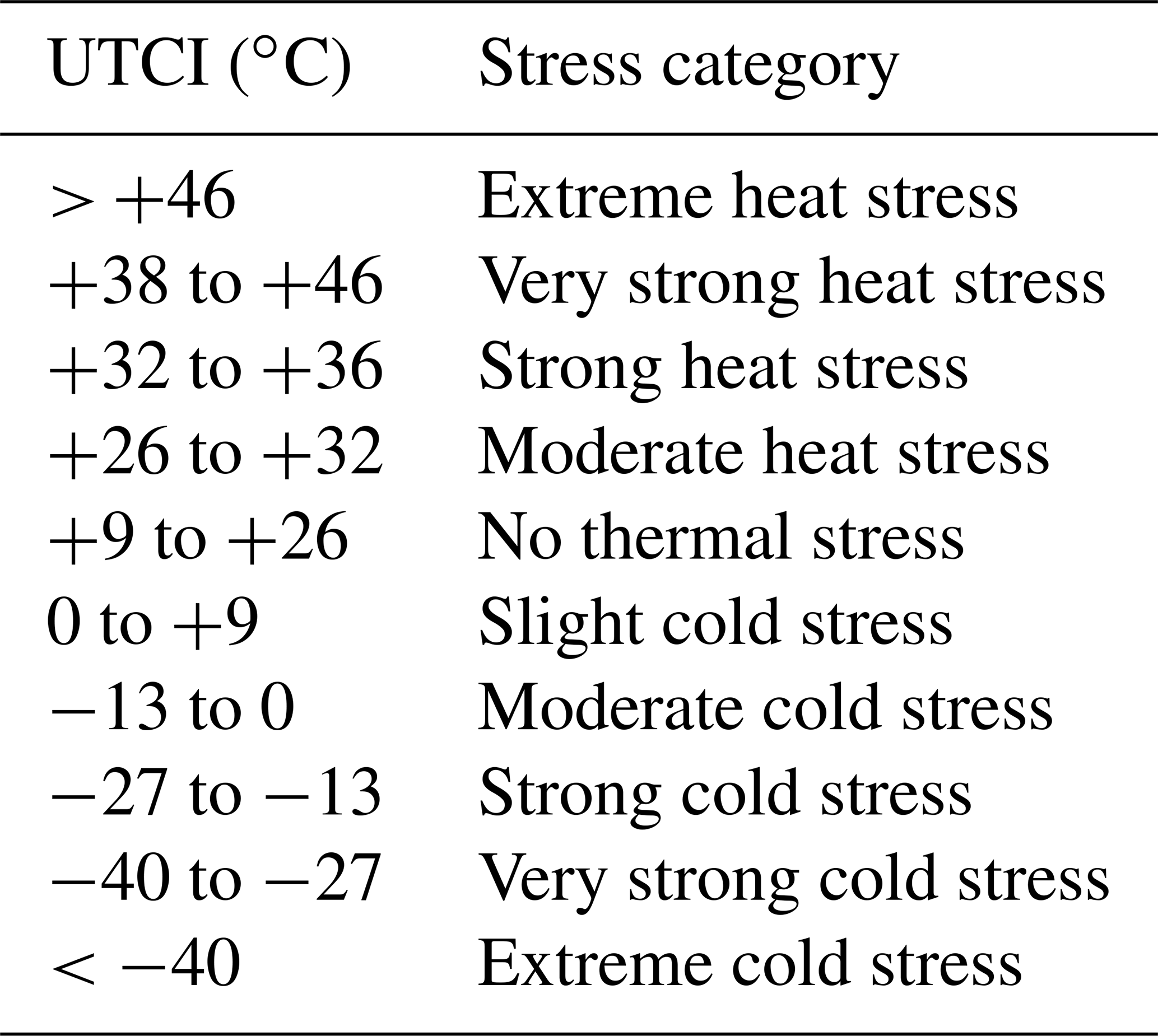
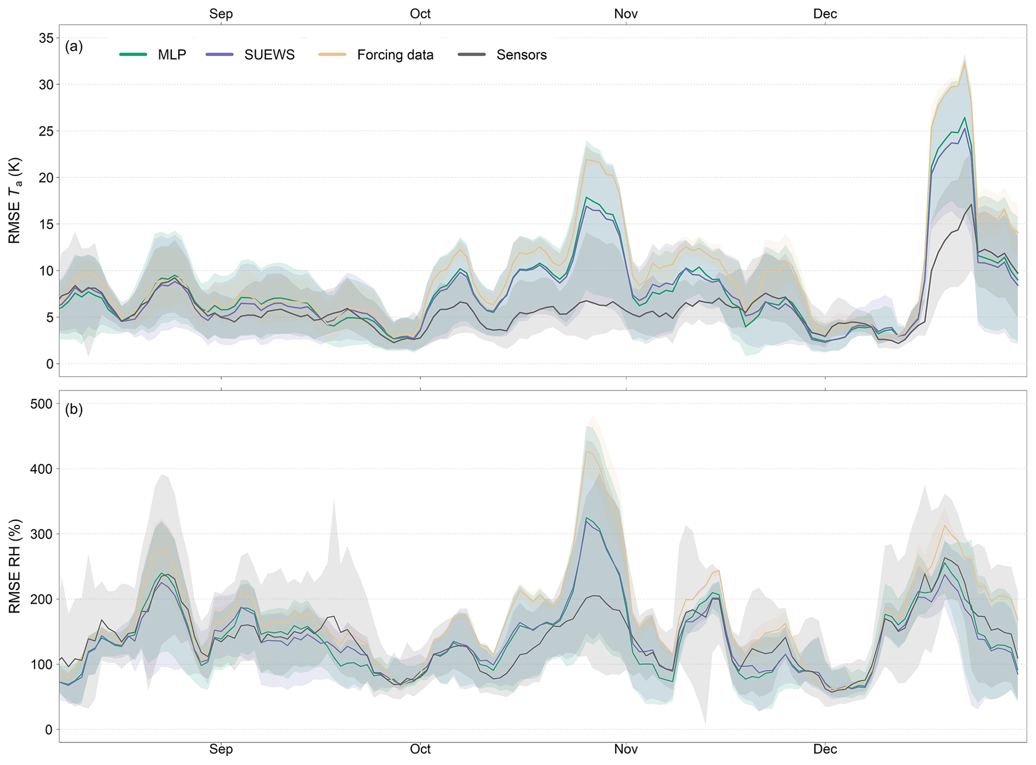
Figure B1 Moving average of RMSEs of T_a (a) and RH (b) from August to December 2022. As reference data, ERA5-Land data are used (Muñoz Sabater, 2019). The window size of the moving average is 7 d. Time series starts with the installation of the first tier-I stations in August 2022. Shaded areas represent 95 % confidence interval.

Table B1 Validation measures of the machine learning models against the numerical models. In contrast to Table 4, where only pointwise comparisons are made, this table shows the mean, MAE, MBE, RMSE, and R² for the entire test area (spatial comparison) for 2022.

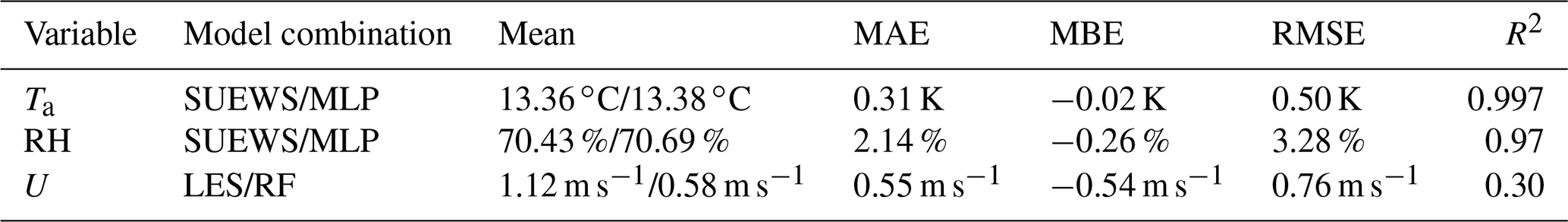
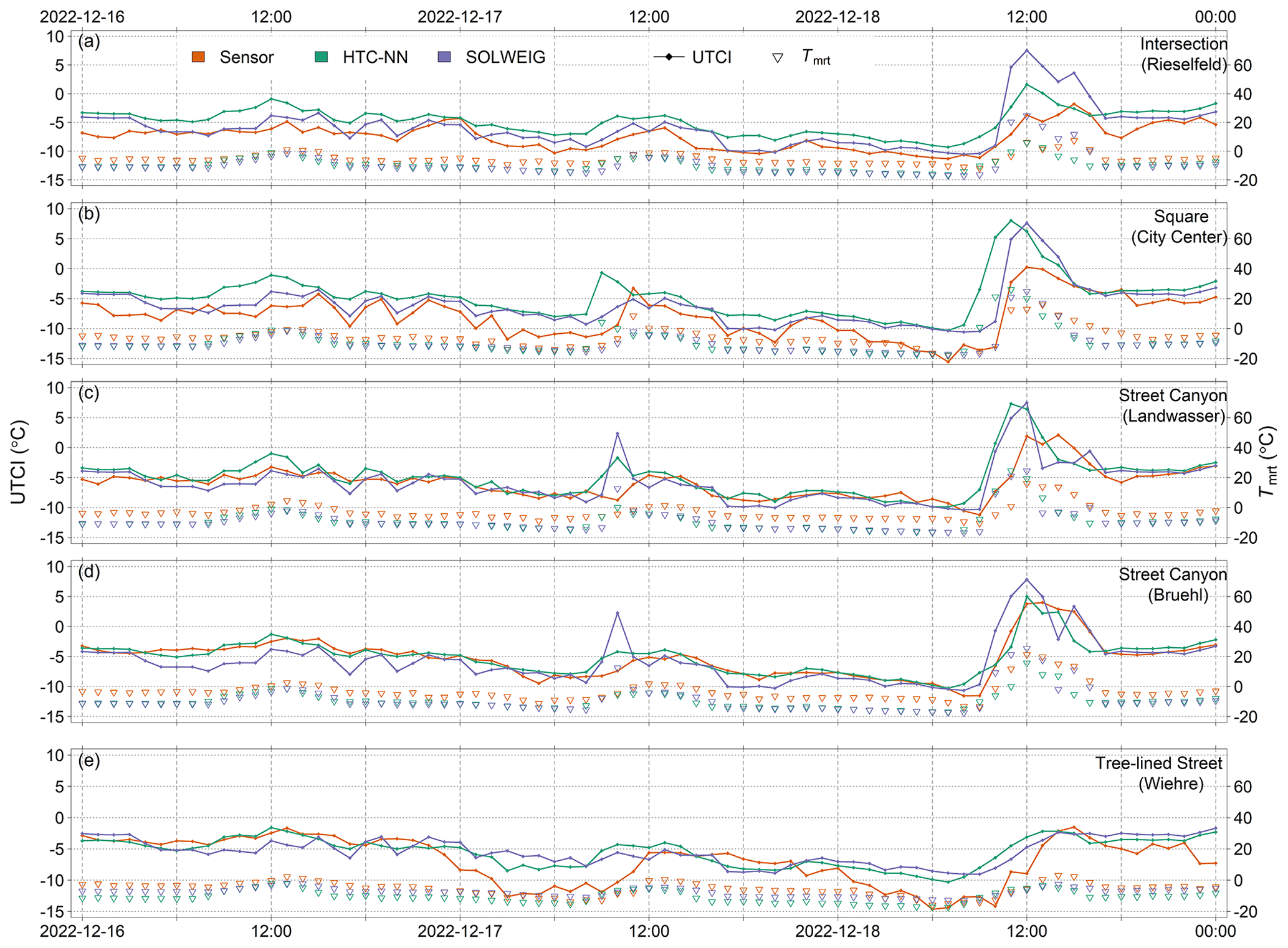
Figure B2 Modelled and measured UTCI at five tier-I stations (a–e) during a cold front in December 2022.

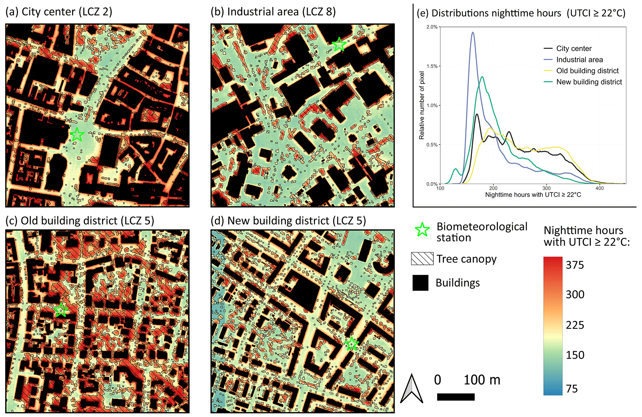
Figure B3 Four 500 × 500 m subsets of different urban neighbourhoods of the city of Freiburg. Average nighttime hours with a UTCI ≥ 22 °C are shown. Panel (a) shows the city centre of Freiburg, panel (b) shows an industrial area in the north of Freiburg, panel (c) shows a district with old buildings and dense or mature tree stock, and panel (d) shows a building district built after the year 1995. Panel (e) shows the distributions of (a)–(e). Note, colouring is in accordance with predicted UTCI quantiles. The spatial resolution is 1 × 1 m, and the time period is 2019–2022.