Perspectives of physics-based machine learning strategies for geoscientific applications governed by partial differential equations

An accurate assessment of the physical states of the Earth system is an essential component of many scientific, societal, and economical considerations. These assessments are becoming an increasingly challenging computational task since we aim to resolve models with high resolutions in space and time, to consider complex coupled partial differential equations, and to estimate uncertainties, which often requires many realizations. Machine learning methods are becoming a very popular method for the construction of surrogate models to address these computational issues. However, they also face major challenges in producing explainable, scalable, interpretable, and robust models. In this paper, we evaluate the perspectives of geoscience applications of physics-based machine learning, which combines physics-based and data-driven methods to overcome the limitations of each approach taken alone. Through three designated examples (from the fields of geothermal energy, geodynamics, and hydrology), we show that the non-intrusive reduced-basis method as a physics-based machine learning approach is able to produce highly precise surrogate models that are explainable, scalable, interpretable, and robust.

1 Introduction

Applications in geosciences dealing with land surface and subsurface environments cover a broad range of disciplines and Earth system compartments comprising lithosphere (including deep reservoirs), groundwater, soil, and the land surface. Subsurface environment applications typically deal with the management of natural resources such as subsurface water stored in soils and aquifers (e.g., water supply, contamination) as well as energy (e.g., geothermal energy, hydrocarbons) that require an in-depth understanding of the governing physical, chemical, and biological principles. In addition, subsurface environments are heterogeneous across a variety of spatial scales, and processes in these environments are typically complex, highly nonlinear, and time-dependent. Spatial scales may range from the nanoscale to the basin and continental scale. Despite the enormous variation in applications in terms of scale and processes, there are underlying common principles. Many of these processes are governed by partial differential equations (PDEs) and are embedded in continuum physics approaches (Bauer et al., 2021; Bergen et al., 2019). In this study, we focus on subsurface applications from the fields of geodynamics, hydrology, and geothermal energy to showcase various methods that are applied in applications which are characterized by data sparsity and difficult accessibility for sampling and measuring states and fluxes as well as for mapping the spatial organization of key subsurface properties.

We focus on continuum PDEs and examine how to accelerate the numerical solution of PDEs that arise from geoscientific applications combining methods from the field of projection-based model order reduction (Benner et al., 2015) and machine learning. Our decision to focus on the aspect of accelerating the solution of PDEs stems from the fact that this is essential in geoscientific applications that aim at improving the understanding of the Earth system with its associated physical processes. An improved understanding requires extensive parameter estimation studies, sensitivity analyses, and uncertainty quantification, which are computationally expensive for many geoscientific PDE-based models (Degen et al., 2022c). This problem is further increased by the circumstance that the governing PDEs are becoming more and more complex as our understanding of the physical processes and their coupling increases. As an example, geothermal studies moved from a purely thermal system to a coupled thermo–hydro–mechanical and, depending on the scale, also a chemical system (e.g., Gelet et al., 2012; Jacquey and Cacace, 2020b; Kohl et al., 1995; Kolditz et al., 2012; O'Sullivan et al., 2001; Stefansson et al., 2020; Taron and Elsworth, 2009). Recent studies include more advanced considerations of the mechanical components, yielding nonlinear hyperbolic PDEs (e.g., Gelet et al., 2012; Jacquey and Cacace, 2017, 2020b, a; Poulet et al., 2014).

The more complex PDEs allow a better characterization of the physical processes in the subsurface. However, they also lead to several challenges.

• Challenge 1. In geoscientific applications, one primary interest is to determine which parameters (e.g., rock and fluid properties) influence the state distribution (e.g., temperature, pressure, stress) to what extent. This question can be addressed through sensitivity analyses, which are categorized into local and global sensitivity analysis (SA) (Wainwright et al., 2014). Local SAs are computationally fast and require only a few simulations. However, they neither return information on the parameter correlation nor allow the exploration of the entirety of the parameter space (Wainwright et al., 2014; Sobol, 2001). Global SAs overcome these issues but are computationally challenging because they demand numerous simulations (Degen et al., 2021b; Degen and Cacace, 2021).

• Challenge 2. Geoscientific and geophysical investigations are often subject to various sources of uncertainty. To assess these uncertainties, stochastic descriptions of the PDEs or probabilistic inverse methods such as Markov chain Monte Carlo are commonly employed. However, these methods have in common that they require solving many forward evaluations, yielding an even more computationally demanding problem (Rogelj and Knutti, 2016; Stewart and Lewis, 2017).

• Challenge 3. Often, PDE-based systems are required for predictions and real-time applications (Bauer et al., 2021; Sabeena and Reddy, 2017). Hence, there is the need to solve PDEs fast. This imposes further difficulties since the simulations for fully coupled nonlinear hyperbolic PDEs are too demanding to allow such fast applications. Therefore, they currently have only limited applicability in many geoscientific research areas (Bauer et al., 2021; Bergen et al., 2019; Willcox et al., 2021).

These challenges have one important aspect in common: they require multiple or fast simulations. If a single simulation already requires a long simulation time, then addressing these challenges becomes difficult to prohibitive.

In this work, we focus on the utility of surrogate models as a way to speed up PDE-based simulations of the physical state in geoscientific problems. In particular, we determine how surrogate models (sometimes also referred to as meta models) can be employed to obtain precise predictions at a reduced computational cost. With the increasing interest in machine learning and the availability of various physics-driven approaches, it is becoming apparent that we need to clarify which requirements we have for our surrogate models. Machine learning has become very popular and powerful in application fields where a vast number of data are available (Baker et al., 2019; Willcox et al., 2021). However, Baker et al. (2019) also stated in their report to the United States Department of Energy that machine learning models need to be scalable, interpretable, generalizable, and robust to be attractive for scientific applications, which is also stated in Willcox et al. (2021). This is important not only for scientific machine learning models but also for surrogate models in general.

• Requirement 1.1, physical scalability. The system resolutions are constantly increasing since one wants to resolve models with higher and higher resolutions in space and time (Bauer et al., 2021; van Zelst et al., 2022). This increase in numerical system size, which is, for instance, noticeable by the increase in degrees of freedom, yields a computationally demanding problem. As an example in geodynamic simulations, one is interested both in large- and small-scale deformations simultaneously. For the time component, variations of the order of milliseconds (seismic cycle) and variations of the order of millions of years (basin- and plate-scale geodynamics) are of interest. In hydrological problems, capturing the spatial small-scale heterogeneity of the surface and subsurface, the short-term nature of meteorological forcing (hours to days), and the long-term nature of subsurface fluxes (tens of years and longer) poses similar challenges (Blöschl and Sivapalan, 1995; Condon et al., 2021; Fan et al., 2019; Paniconi and Putti, 2015). This results in computational expensive problems (van Zelst et al., 2022), which often require high-performance computing (HPC) infrastructures even for solving a single forward problem.

• Requirement 1.2, performance scalability. Porting applications to HPC infrastructures is another major requirement, which requires the rewrite of major parts of the software packages (Alexander et al., 2020; Artigues et al., 2019; Baig et al., 2020; Bauer et al., 2021; Bertagna et al., 2019; Lawrence et al., 2018; Gan et al., 2020; Grete et al., 2021; Hokkanen et al., 2021). Therefore, one important aspect is to evaluate how physics-based machine learning methods can help in the transition to modern HPC infrastructures.

• Requirement 2, interpretability. Another main requirement is to produce surrogate models that maintain the characteristic of PDE solutions and the original structure of the governing principles (i.e., that they map from model parameters to state information). Related to this is the consideration of nonlinear problems (Grepl, 2012; Hesthaven and Ubbiali, 2018; Reichstein et al., 2019; van Zelst et al., 2022), which, in the field of geosciences, is often related to the consideration of mechanical or complex flow effects. Such nonlinear problems result in extensive computation times because of extra iterations in the numerical solve (van Zelst et al., 2022).

• Requirement 3, generalizability. Furthermore, it is important that the approaches apply to various disciplines and are not restricted to single applications only. To enable a transfer between disciplines it is important to provide accessible solutions. Often software packages are developed in-house and are not available to the entire community.

• Requirement 4, robustness. The last requirement is robustness. It is critical that the solutions produced by the surrogate models are consistent for different levels of accuracy. As an example, it is not desired to have a surrogate model that predicts lower accuracy for a diffusion-dominated solution and slightly increased accuracy for an advection-dominated solution.

The paper is structured as follows: we present the PDEs considered in this study first (see Sect. 2). Afterwards, we present the concept of data-driven, physics-based approaches and physics-based machine learning in the same section. In Sect. 3, we present three designated case studies, from the field of geothermal energy, geodynamics, and hydrology, to illustrate the potential of physics-based machine learning. This is further emphasized in Sect. 4, where we evaluate how physics-based machine learning can address various challenges commonly occurring in the field of geosciences. We conclude the paper in Sect. 5.

2 Surrogate modeling methods

In the following, we introduce different surrogate model techniques to address the challenges presented in Sect. 4. Thereby, the focus is on inverse applications, uncertainty quantification methods, global sensitivity analyses, and other methods concerned with parameter estimation.

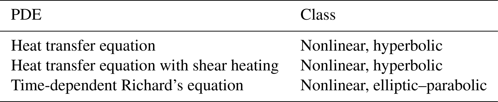
Surrogate models can be constructed with physics- and data-driven approaches (Fig. 1a, b). Physics-driven approaches preserve the governing equations, meaning that they, for instance, conserve mass, momentum, and energy in the same way as the original discretized version. They also maintain the characteristic that for a given set of model parameters (e.g., material properties), they produce information about the state variables (e.g., temperature, pressure) at, for instance, every node of the discretized model. But they are limited in the complexity that they can capture (Fig. 1a). We focus here on hyperbolic and/or nonlinear PDEs as these pose computational challenges in physics-based methods, as outlined above. We will not cover linear elliptic and linear parabolic PDEs for which we advise using pure physics-based approaches. These can provide error bounds in addition to the surrogate model, allowing us to obtain objective guarantees of the approximation quality. In Table 1, we list the PDEs used throughout the paper and their respective classes.

Table 1 List of partial differential equations and their respective classes used throughout the paper.

Within the physics-driven approaches, we focus on techniques that allow a retrieval of the entire state. Projection-based model order reduction techniques, such as proper orthogonal decomposition (POD), balanced truncation, and the reduced-basis method, belong to this class (Benner et al., 2015). We discuss physics-based approaches in detail in Sect. 2.1. Machine learning techniques are a common example of data-driven approaches (Baker et al., 2019; Bauer et al., 2021; Willcox et al., 2021). They have the advantage of capturing the full complexity of the model at hand but lose the information about the physical system (Fig. 1b). Examples of other data-driven techniques are kriging (Gaussian processes), polynomial chaos expansion, and response surfaces (e.g., Miao et al., 2019; Mo et al., 2019; Navarro et al., 2018). Data-driven methods are described in Sect. 2.2. The last category is physics-based machine learning, which combines aspects of both physics-based and data-driven techniques to overcome the limitations of the individual approaches (Fig. 1c). A detailed overview of this technique is provided in Sect. 2.3.

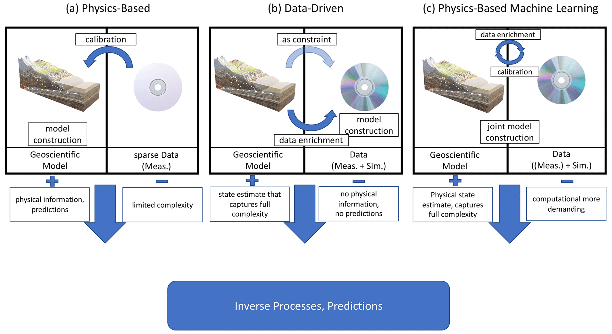
Figure 1 Schematic comparison of physics-based, data-driven, and physics-based machine learning methods for the construction of surrogate models. “Meas.” indicates measured (e.g., well data, surface observations) and “Sim.” indicates simulated. The boxes with a + list advantages, and the boxes with a − list disadvantages of the method above.

2.1 Physics-based surrogate modeling and model order reduction

Model order reduction (also called reduced-order modeling) has been extensively used in various application fields, such as groundwater (Ghasemi and Gildin, 2016; Gosses et al., 2018; Rousset et al., 2014) and thermal studies (Rizzo et al., 2017). The idea is to find a low-dimensional representation of the original high-dimensional problem, while maintaining the input–output relationship. This low-dimensional representation allows a fast computation, enabling, in turn, probabilistic inverse methods and other forward-intensive algorithms. Commonly known methods of projection-based model order reduction techniques are proper orthogonal decomposition (POD) (Benner et al., 2015; Hesthaven et al., 2016; Volkwein, 2011), the reduced-basis (RB) method (Hesthaven et al., 2016; Prud'homme et al., 2002; Quarteroni et al., 2015), and balanced truncation (Antoulas, 2005). In the following, we will briefly introduce the POD and RB methods since they are relevant for the remaining case studies. For a more detailed overview of projection-based model order reduction, we refer to Benner et al. (2015).

POD is the probably most widely used projection-based model order reduction technique. For the construction of the reduced model, we first calculate snapshots. Snapshots are state distributions for different parameters (e.g., rock properties) and/or different time steps. Afterwards, we perform a singular value decomposition. The reduced basis is obtained by keeping the singular vectors corresponding to the largest singular values. The resulting orthonormal POD basis is turned into the reduced model through a Galerkin projection (Benner et al., 2015; Hesthaven et al., 2016; Volkwein, 2011). We categorize the POD as a physics-based method since through the projection the PDE is translated from the space of the spatial coordinates to the material properties. In the case that all POD modes are used this leads to an equivalent representation. The Galerkin projection needs access to the stiffness matrix and load vector and hence direct access to the discretized version of the PDE. Note that a POD can also be directly applied to, for instance, image data that have not been constructed by PDEs. However, in this case, no Galerkin projection would be applied. In the geoscience community, the POD method has been used in, for instance, thermal applications (Rousset et al., 2014) and groundwater studies (e.g., Ghasemi and Gildin, 2016; Gosses et al., 2018; Rizzo et al., 2017; Vermeulen et al., 2004; Vermeulen and Heemink, 2006).

Another physics-based method is the RB method. The idea of RB is similar to the principle of POD. The main difference is the construction of the reduced basis. In RB the selection of the snapshots is often performed via a greedy algorithm as the sampling strategy. The greedy algorithm chooses the solution that adds the highest information content at each iteration (Bertsimas and Tsitsiklis, 1997; Veroy et al., 2003). Afterwards, the orthonormalized snapshots are added to the reduced basis and the reduced model is again obtained via a Galerkin projection (Benner et al., 2015; Hesthaven et al., 2016; Prud'homme et al., 2002; Quarteroni et al., 2015). Since this version of the RB method does not calculate the snapshots in advance but calculates them “on the fly” it performs slightly better for higher-dimensional parameter spaces (Jung, 2012). However, for the efficient construction of the reduced basis, an error bound or estimator is required. Currently, no efficient error bounds for hyperbolic PDEs exist, limiting the applicability of the method. The RB method is a physics-based method since, as described for the POD above, it is a projection method, and the Galerkin method requires the discretized version of the PDE.

A note of caution: the combination of the POD and the Galerkin projection step is sometimes referred to as POD (Swischuk et al., 2019) only and sometimes as POD-Galerkin (Busto et al., 2020).

Both the POD and the RB method have limitations when considering complex geophysical problems. Both methods aim at an affine decomposable problem, meaning that our problem is decomposable into a parameter-dependent and parameter-independent part. This requirement is naturally given for linear but not for nonlinear problems. Methods such as the empirical interpolation method (Barrault et al., 2004) exist to extend the methods for the nonlinear case, but their performance for high-order nonlinearities is limited.

Our choice to mostly rely on physics-based methods stems from the fact that understanding the physical processes is a central component in geosciences. Physics-driven methods are ideal for predictions and risk assessments, but they also have the major disadvantage of being computationally too demanding for complex coupled subsurface processes. In the literature, this can often be observed indirectly. For example, in geothermal applications basin-scale applications usually consider a hydrothermal system, whereas reservoir-scale applications also incorporate the mechanical and/or chemical processes (e.g., Freymark et al., 2019; Gelet et al., 2012; Jacquey and Cacace, 2017, 2020b, a; Kohl et al., 1995; Kolditz et al., 2012; Koltzer et al., 2019; O'Sullivan et al., 2001; Poulet et al., 2014; Stefansson et al., 2020; Taron and Elsworth, 2009; Taron et al., 2009; Vallier et al., 2018; Wellmann and Reid, 2014). Another example is magnetotellurics (MT). The inversion of MT data is very costly; hence, most inversions are performed in 1D or 2D (e.g., Chen et al., 2012; Conway et al., 2018; Jones et al., 2017; Rosas-Carbajal et al., 2014). 3D MT inversion is challenging even with HPC infrastructures (Rochlitz et al., 2019; Schaa et al., 2016). How to accelerate solving the Maxwell equations through the reduced-basis method and simultaneously achieve efficient error estimates or bounds has been shown fundamentally in, e.g., Chen et al. (2010), Hammerschmidt et al. (2015), Hess and Benner (2013a), Hess and Benner (2013b), and Hess et al. (2015). The potential of the reduced-basis method is well illustrated in Manassero et al. (2020), where the authors perform an adaptive Markov chain Monte Carlo run for an MT application using the reduced-basis method.

2.2 Data-driven techniques

In applications where we have a huge amount of data (e.g., earthquake and seismic applications) and only limited knowledge of the physical processes, data-driven approaches such as machine learning are superior to purely physics-based methods (Bergen et al., 2019; Raissi et al., 2019). Machine learning approaches are powerful in discovering low-dimensional patterns and in reducing the dimensionality of the model. Hence, they would be ideal for surrogate models. A review of the state and potential of machine learning techniques for the solid Earth community is provided in Bergen et al. (2019) focusing on data-rich applications such as the analyses of earthquakes. The applied methods in this field comprise, for instance, (deep) neural networks, random forest, decision trees, and support vector machines. However, open questions remain about the reliability, the explainability of the models, the robustness, and the rigorousness of how much the underlying assumptions have been tested and validated (Baker et al., 2019; Willcox et al., 2021). This is critical in applications such as risk assessment, where we need to provide guarantees and confidence intervals for our predictions. Another issue is that data-driven approaches such as machine learning are problematic in terms of robustness and have no proven convergence if applied to the so-called “small data” regime (Raissi et al., 2019). Raissi et al. (2019) define the small data regime as a regime where the collection of data becomes too expensive and thus conclusions have to be drawn on incomplete datasets.

This is especially critical for the application field of solid Earth, where we are classically concerned with a lack of data. Hence, this field does not allow straightforward applicability of data-driven approaches. Furthermore, in this field, we need to perform predictions and risk assessments. Therefore, black-box approaches, such as machine learning, pose a major challenge in how to provide guarantees and how to obtain interpretable models (Baker et al., 2019; Willcox et al., 2021).

Some data-driven methods assume that we are interested in a quantity of interest and not in the entire state distribution. Possible quantities of interest are the value of the state variable at a certain location in space or the amount of substance that is accumulated over time in a certain region. Note that this class of methods allows a violation of the governing conservation laws since it commonly uses statistical methods for the construction of the surrogate model (Bezerra et al., 2008; Cressie, 1990; Khuri and Mukhopadhyay, 2010). Typical methods used in the field of geosciences are kriging, polynomial chaos expansion, and response surfaces (Baş and Boyacı, 2007; Bezerra et al., 2008; Frangos et al., 2010; Khuri and Mukhopadhyay, 2010; Miao et al., 2019; Mo et al., 2019; Myers et al., 2016; Navarro et al., 2018). We will not further discuss this class of methods since in this paper we focus on applications that are not only interested in a quantity of interest but also in the entire state distribution. For an overview of data-driven machine learning techniques, we refer to Jordan and Mitchell (2015), Kotsiantis et al. (2007), and Mahesh (2020).

2.3 Physics-based machine learning

Data-driven methods are a nonideal choice in the Earth sciences because they do not provide an understanding of the underlying subsurface processes (Reichstein et al., 2019). Furthermore, they require more data than physics-based methods (Willcox et al., 2021), which is relevant because some applications fields such as geodynamics and geothermal applications are characterized by data sparsity. However, physics-based methods are also not applicable for complex coupled processes since they do not capture the full complexity of the problem.

This is the reason why we introduce the concept of physics-based machine learning. Note that we discuss the potential of these methods for applications where primarily physical knowledge is available (in the form of PDEs) with very sparse to no data. The discussion would be different in a data-dominated application. Physics-based machine learning uses a combination of data-driven and physics-based techniques, as schematically shown in Fig. 1. For solving PDEs Willard et al. (2020) distinguish various techniques, comprising the categories of physics-guided loss functions, physics-guided architectures, and hybrid models. These various approaches are already compared in several papers (e.g., Faroughi et al., 2022; Swischuk et al., 2019; Willard et al., 2020). However, they focus on applications where substantially more data are available than in most subsurface applications. Therefore, we shift the focus to applications with very sparse datasets. This impacts the potential of physics-based machine learning methods differently, depending on the paradigm used to combine physics- and data-based methods. So, instead of presenting numerous of these techniques in detail, as already done in the aforementioned papers, we want to discuss the different paradigms that exist. Here, we identify two end-member cases: (i) physics-guided loss functions and (ii) hybrid models.

In physics-guided loss function methods, the idea is to use a data-driven approach and incorporate the physics in the loss function to force the system to fulfill the physical principles. They have a better performance for the small data regime since the physical constraints regularize the system and they constrain the size of admissible solutions (Raissi et al., 2019). Within the field of physics-guided loss functions various different approaches are available (e.g., Bar-Sinai et al., 2019; De Bézenac et al., 2019; Dwivedi and Srinivasan, 2020; Geneva and Zabaras, 2020; Karumuri et al., 2020; Meng and Karniadakis, 2020; Meng et al., 2020; Pang et al., 2019, 2020; Peng et al., 2020; Raissi et al., 2019; Shah et al., 2019; Sharma et al., 2018; Wu et al., 2020; Yang et al., 2018; Yang and Perdikaris, 2018; Yang et al., 2020; Zhu et al., 2019). For the following, we focus on the method of physics-informed neural networks (PINNs) as an example.

The second class of physics-based machine learning techniques that we present in more detail are hybrid models. In this technique, the physics are not added as a constraint in the loss function, but instead we perform both a physics-based and a data-driven approach. Often the physics-based method is executed first and the output serves as an input to the machine learning approach (Willard et al., 2020; Hesthaven and Ubbiali, 2018; Swischuk et al., 2019). Also, for this class of methods, various methods are available (Hesthaven and Ubbiali, 2018; Malek and Beidokhti, 2006; Swischuk et al., 2019; Wang et al., 2019); here we focus on the non-intrusive RB method.

Note that both methods act as examples to better illustrate the different concepts used for combining physics- and data-based approaches. Numerous other methods exist such as the physics-encoded neural network (PeNN) (Chen et al., 2018a; Li et al., 2020; Rao et al., 2021), physics-encoded recurrent-convolutional neural network (PeRCNN) (Rao et al., 2021), the Fourier neural operator (FNO) (Li et al., 2020), and DeepONets (Lu et al., 2021). We will not discuss these in detail but shortly explain their relations to the two paradigms, represented by PINNs and the non-intrusive RB method.

2.3.1 Physics-guided loss functions and physics-informed neural networks

PINNs overcome the shortcomings of machine learning techniques by including physics in the system. The principle is that in applications where we lack data we often have other sources of information, including domain expert knowledge and physical laws (e.g., conservation and empirical laws). By including these additional sources into machine learning the problem is regularized and the set of admissible solutions greatly reduced, yielding significantly improved performance of the algorithm (Raissi et al., 2019). The idea of including physical knowledge is well known for Gaussian processes. However, Gaussian processes have only limited applicability for nonlinear problems (Raissi et al., 2017; Raissi and Karniadakis, 2018). Therefore, PINNs rely on neural networks which are known for their good performance in the estimation of nonlinear functions (Raissi et al., 2019).

Figure 2 Schematic representation of a physics-informed neural network.

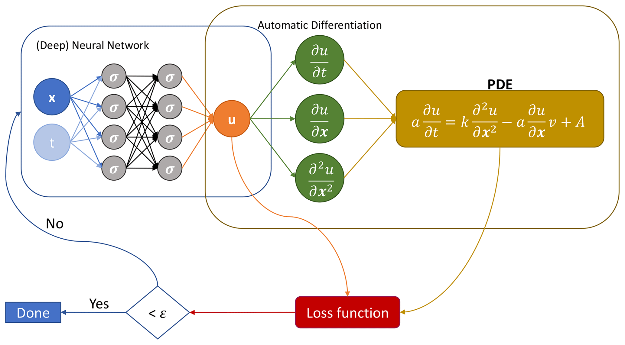
In Fig. 2, we show the setup of a PINN schematically. The first step is to create a (deep) neural network with space and time as inputs. The network generates a model for the state variable u. Through automatic differentiation, we obtain the spatial and temporal derivatives, which, in turn, are used in the calculation of the PDE. We learn the shared parameters of the network and the PDE by minimizing a joint loss function as presented in Eq. (1) (Raissi et al., 2019):

$$\begin{array}{}\text{(1)}& \begin{array}{rl}& \mathrm{MSE}={\mathrm{MSE}}_u+{\mathrm{MSE}}_f,\\ \mathrm{where}& {\mathrm{MSE}}_u={\displaystyle \frac{\mathrm{1}}{N_u}}\sum _{i=\mathrm{1}}^{N_u}|u\left(t_u^i,x_u^i\right)-u^i{\mathrm{|}}^{\mathrm{2}},\\ \text{and}& {\mathrm{MSE}}_f={\displaystyle \frac{\mathrm{1}}{N_f}}\sum _{i=\mathrm{1}}^{N_f}|f\left(t_f^i,x_f^i\right){\mathrm{|}}^{\mathrm{2}}.\end{array}\end{array}$$

Here, MSE stands for mean squared error, u(t,x) denotes the variable with the training data $\mathit{\{}{t}_u^i,x_u^i,u^i{\mathit{\}}}_{i=\mathrm{1}}^{N_u}$, and $\mathit{\{}{t}_f^i,x_f^i,{\mathit{\}}}_{i=\mathrm{1}}^{N_f}$ represents the collocation points for our PDE f(x,t). The subscript u refers to the constraints for the boundary and initial conditions and the subscript f to the PDE constrains. Consequently, the MSE_u minimizes the difference between the data u and the simulated data at the collocation points (for the boundary and initial conditions). The MSE_f enforces the structure of the PDE at selected collocation points. Through the terms $\frac{\mathrm{1}}{N_u}$ and $\frac{\mathrm{1}}{N_f}$, we can weight the components of the loss function depending on, for instance, the amount of available data and physical knowledge.

PINNs are frequently used due to their high flexibility and straightforward implementation. They are used as a state estimation technique since they can recover the entire state from a given set of observations. PINNs face problems in high-frequency and multiscale feature scenarios (Wang et al., 2022). Further disadvantages of PINNs are that the PDE is used as a constraint (among other constrains) and is enforced at a limited number of selected points only. Chuang and Barba (2022) point out that PINNs also have disadvantages concerning their computational efficiency. Due to the usage of automatic differentiation many residuals need to be evaluated, leading to high computational costs. Additionally, in their tested computational fluid dynamics applications, losses close to zero needed to be minimized, yielding performance and convergences issues. This problem is also expected for a wide range of geoscientific applications. Lastly, Chuang and Barba (2022) reported that PINNs did not reproduce the desired physical solution in all of their benchmark examples. Therefore, the applicability of PINNs should be investigated prior to their use.

Numerous variations of PINNs are available, and we provide an overview of the following:

• B-PINNs (provide a built-in uncertainty quantification, Yang et al., 2020)

• fPINNs (for fractional PDEs, Pang et al., 2019)

• nPINNs (for a nonlocal universal Laplace operator, Pang et al., 2020)

• PPINNs (offer a time parallelization, Meng et al., 2020)

• sPINNs (for stochastic PDEs, Chen et al., 2019)

• XPINNs (offer an efficient space–time decomposition, Jagtap and Karniadakis, 2020)

PINNs directly provide an estimate of the state and do not preserve the input–output relationship (e.g., from model parameters to state information) of our original physical problem. Hence, we no longer have a model that takes rock and fluid properties as input and produces estimates of, for instance, the temperature or pressure as our output. Additionally, PINNs assume that observation data might be sparse but are available. In many geoscientific applications, we have an extremely sparse dataset and sometimes no direct observation data. Just as an example, if we want to investigate the formation of a sedimentary basin, we have only direct measurements for the present state. For the past, we have at best indirect measurements at hand. Consequently, we do not have enough data to utilize the PINN. In order to compensate, an enrichment of the dataset by, for instance, numerical simulations is needed. However, these numerical simulations are the results of PDEs. So, the natural question would be why we do not use a method that builds upon the principles of PDEs rather than using the PDEs as a constraint. Therefore, we do not see benefits in employing PINNs for applications that have nearly no data, which is the case for the geothermal and geodynamic applications we consider in this paper. For subsurface hydrological data the situation is better since exhaustive data for the land surface are available. However, the data are commonly of low quality (e.g., coarse, with systematic biases and measurement gaps). This yields similar problems for the PINNs as in the “no data” case. Hence, we focus in the remaining part of the paper on another physics-based machine learning technique, namely the non-intrusive RB method, which we present in the next section.

2.3.2 Hybrid methods – non-intrusive reduced-basis method

The non-intrusive RB method originates from the model order reduction community. Model order reduction and machine learning have huge similarities. For example, proper orthogonal decomposition is very closely connected to principal component analysis (Swischuk et al., 2019). Swischuk et al. (2019) pointed out that the difference between the methods has historical reasons. Model order reduction methods have been developed by the scientific computing community to reduce the high-dimensional character of typical scientific applications. In contrast, machine learning originates from the computer science community aiming at generating low-dimensional representations through black-box approaches (Swischuk et al., 2019).

The first method that we presented, physics-informed neural networks, can be seen as a machine-learning method, where we use physics to constrain our system. On the other hand, the non-intrusive RB approach can be seen as a modification of the model order reduction techniques of POD and RB using data-driven approaches. The major difference between the methods is the question of what we learn from the algorithm. For PINNs, we are learning the operators themselves. In contrast, the non-intrusive RB method derives a mapping between the input parameters (e.g., rock properties) and the output (e.g., temperature and pressure distribution) (Swischuk et al., 2019).

The idea behind model order reduction is that the reduced solution u_L(x;μ) can be expressed as the sum of the product of the basis functions ψ(x) and the reduced coefficients u_rb(μ). Here, x defines the spatial coordinates and μ the parameters. The procedure is described in Eq. (2) (Hesthaven and Ubbiali, 2018):

$$\begin{array}{}\text{(2)}& u_L\left(\mathit{x};\mathit{\mu }\right)=\sum _{l=\mathrm{1}}^L{u}_{\mathrm{rb}}^{\left(l\right)}\left(\mathit{\mu }\right){\mathit{\psi }}_l\left(\mathit{x}\right).\end{array}$$

So, for the construction of the surrogate model, two steps are required. First the basis functions are determined, and afterwards the reduced coefficients are conventionally determined by a Galerkin projection. In Sect. 2.1, we present two projection-based model order reduction techniques. The disadvantage of the presented methods is that they have only limited applicability to nonlinear PDEs (Hesthaven and Ubbiali, 2018; Wang et al., 2019). Furthermore, they require access to the decomposed stiffness matrix and load vector. However, this retrieval is sometimes prevented by the forward solver (i.e., in commercial software packages) (Peherstorfer and Willcox, 2016). Limitations regarding both nonlinearity and the software arise from this intrusive Galerkin projection.

To overcome the problem with the projection recent advances have replaced the intrusive projection with a non-intrusive approximation (Hesthaven and Ubbiali, 2018; Wang et al., 2019). Hesthaven and Ubbiali (2018) and Wang et al. (2019) propose a (deep) neural network for learning the reduced coefficient. Other approaches including interpolation and machine learning methods have been explored for this purpose (Swischuk et al., 2019). Swischuk et al. (2019) compare four machine learning methods, namely neural networks, multivariate polynomial regression, k-nearest neighbors, and decision trees, for the determination of the reduced coefficients in aerodynamic and structural applications. Audouze et al. (2009, 2013) and Wirtz et al. (2015) use Gaussian process regression to determine the reduced coefficients. Another strategy is proposed in Mainini and Willcox (2015), where the reduced coefficients are learned by an adaptive mixture of self-organizing maps and response surfaces.

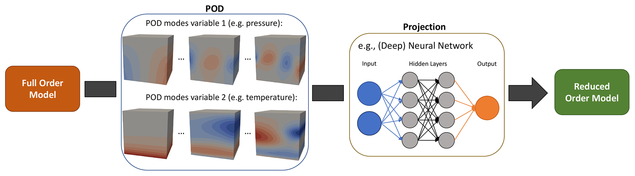
Figure 3 Schematic representation of the non-intrusive reduced-basis method with a proper orthogonal decomposition sampling strategy.

Due to the different methods for obtaining the reduced coefficients, the commonly used greedy sampling strategy of the intrusive RB method (Hesthaven et al., 2016; Veroy et al., 2003) has to be modified. For the selection of basis functions, we can either use a POD (Hesthaven and Ubbiali, 2018; Wang et al., 2019) or a modified greedy sampling strategy (Chen et al., 2018b). In the case of the POD, which is used in this paper, the snapshots (i.e., simulation results for different model parameters) serve as an input and the basis functions as an output. For the second stage, the projection is via a machine learning method. The labels are the different model parameters (e.g., permeability, thermal conductivity), the training data the matrix product of the snapshots and the basis functions, and the outputs the reduced coefficients. Taking the matrix product of snapshots and basis functions means that the dimension of spatial degrees of freedom does not enter into the training of the machine learning model, which has great implications regarding the cost of training these models, as we will detail in Sect. 3.5.

Note that non-intrusive model order reduction is not restricted to the inference of the output states via the input parameters. As an example, Peherstorfer and Willcox (2016) developed a data-driven operator inference non-intrusive method. However, this method is restricted to low-dimensional nonlinearities for computational reasons (Peherstorfer and Willcox, 2016). As we aim to demonstrate the potential of physics-based machine learning, we chose as an example two techniques: one closer to the community of computer science and the other closer to the community of scientific computing. We do not aim to provide an overview of all possible methods.

Again, we add a note of caution with regard to the terminology. The non-intrusive RB method consists of a sampling and projection step. If we use, for instance, the POD as the sampling method and the NN as the projection method, then this is often referred to as POD-NN (Hesthaven and Ubbiali, 2018) instead of non-intrusive RB. In this paper, we use various machine learning techniques for the projection step. Since this has no general impact on the applicability of physics-based machine learning we use the more general term of non-intrusive RB to avoid unnecessary confusion.

2.3.3 Other physics-based machine learning methods

As discussed before, many physics-based machine learning methods are available, all with their own advantages and disadvantages. Nonetheless, we can identify generally different approaches regarding how to integrate physics into data-driven approaches; see also Willcox et al. (2021). These diverse approaches yield different potential for addressing current challenges faced in subsurface applications, as we will present in Sect. 4. So, in the following, we briefly present other physics-based machine learning methods and how they relate to the two paradigms presented in detail.

The idea behind PeNNs is to hard-encode the prior physical knowledge in the architecture of neural networks. This can be achieved through various methods (Chen et al., 2018a; Li et al., 2020; Rao et al., 2021). One possibility is the PeRCNN, where an optional physics convolution layer is implemented. This means that the method is in between PINNs and the non-intrusive RB method. It is able to overcome some common problems encountered with PINNs since it does not implement physics as one of many possible constraints. However, the method is still a statistical interpolation method and therefore cannot guarantee a preservation of the physics. Regarding the categories that are used in Willard et al. (2020), this method would fall under the category of physics-guided architectures.

Another method that is associated with PeNNs involves FNOs (Faroughi et al., 2022; Li et al., 2020). This method uses Fourier layers instead of the typical layers used in a neural network. Conceptually this is close to the non-intrusive RB method. In the Fourier layers the data are decomposed, similar to the POD step of the non-intrusive RB method. However, the main difference is that FNO is limited to sine and cosine functions. Neural operators are known to require large training datasets (Lu et al., 2022), which is critical in the applications presented here since the generation of the data is often very costly. Furthermore, they are limited when it comes to complex 3D problems (Lu et al., 2022). Another difference to the non-intrusive RB method is that again the approach is embedded into a data-driven scheme. Something similar is the case for DeepONets (Lu et al., 2021), which overcome the requirement of structured data that FNOs have but show conceptually similar limitations as FNOs.

2.3.4 Differences in physics-based machine learning

We provide examples from the field of hydrology and water resource management since machine learning is currently actively being studied in these research fields (Shen et al., 2021; Sit et al., 2020). This is fueled by the promise of ML to unravel information and provide hydrological insights (Nearing et al., 2021) in what can be considered increasingly rich(er) datasets, especially for surface hydrology (in comparison to subsurface hydrology and other subsurface geoscientific applications, such as geodynamics). Typical applications of ML include runoff and flood forecasting, drought forecasting, water quality, and subsurface flows, among many others (see Ardabili et al., 2020; Bentivoglio et al., 2021; Mohammadi, 2021; Sit et al., 2020; Zounemat-Kermnai et al., 2021, for extended reviews on the topic). Many of these applications are based on artificial neural networks (ANNs) and deep learning tool sets which have become accessible to hydrologists thanks to the arrival of well-established and GPU-enabled libraries. It is currently clear that ML offers a wide range of possibilities in hydrology, such as faster-than-real-time forecasting, extracting information from citizen data, parameter inversion, and uncertainty quantification. The idea of ML surrogates is increasingly being exploited in hydrological research (e.g., Bermúdez et al., 2018; Liang et al., 2019; Tran et al., 2021; Zahura et al., 2020; Zanchetta and Coulibaly, 2022).

Physics-based ML is still rare and incipient in hydrology, with efforts largely motivated by overcoming the black-box nature of traditional ML techniques (Jiang et al., 2020; Young et al., 2017) and the need to include physical constraints and theory (Nearing et al., 2021). The techniques to inform ML of the physics, as well as how much of the physics is embedded into the problem, depend on the application and the underlying deterministic model, ranging from ordinary partial differential equations (ODEs) (Jiang et al., 2020) to classical lumped cascade hydrological models (Young et al., 2017), subsurface hydraulic parameter estimation based on nonlinear diffusion equations (Tartakovsky et al., 2020), the Darcy equation (He et al., 2020) and Richards equation (Bandai and Ghezzehei, 2021), and overland flow (Maxwell et al., 2021). It is therefore clear that there is growing momentum and clear potential gains in exploring physics-based ML in hydrological sciences, motivated by methodological, theoretical, and computational factors.

The term physics-based machine learning is used in an increasing number of scientific works; however, the methodologies employed vastly differ. Therefore, we would like to briefly elaborate on the differences between these techniques. Note that this explanation is purely meant to illustrate the usage of the term physics-based machine learning throughout the remaining part of this paper. To our knowledge, there is no unique definition of that term. Furthermore, we will only illustrate the differences between the methodologies presented here. We do not aim to provide a complete overview of all physics-based ML techniques but rather illustrate the various concept associated with the technique in general.

What might be sometimes defined as physics-informed or physics-based approaches are applications whereby the surrogate model is constructed with classical data-driven ML techniques but the data originate from a physical model instead of observation data. In this paper, the definition of physics-based ML is purely based on the methodology. Since the former application is methodology-wise the same as a data-driven approach this would be defined here as a data-driven and not a physics-based ML technique.

The two physics-based ML techniques presented here are PINNs and the non-intrusive RB method. Both methods have similar aims but are vastly different in where and how ML techniques and physics are utilized. PINNs use the physics as an additional constraint in the loss function and do not preserve the original structure of the problem. In contrast, the non-intrusive RB method extracts the main physical characteristics and weights them using an ML technique, while maintaining the input–output relationship.

3 Benchmark studies

Combining both data- and physics-driven techniques allows for robust and reliable (surrogate) models that enable probabilistic inverse processes, which yield a significant improvement in the understanding of the Earth system. For an illustration of the potential that physics-based machine learning has for the community, we present in the following three benchmark studies from the field of geothermal, geodynamical, and hydrological applications. Afterwards, we use these studies to illustrate how physics-based machine learning can help to overcome the challenges introduced at the beginning of the paper.

3.1 General workflow

Before we present three case studies in the next section, we present a general workflow (Fig. 4) and point out some common pitfalls for the data-driven part of the methodology. Although the procedure is developed with the projection part of the non-intrusive RB method in mind, it applies to a wide range of data-driven approaches. For the following workflow, we assume that a geometrical and physical model is already available. Hence, we assume that the model is already tested for single forward simulations.

• 1.

  At the beginning of the procedure, we need to define the training and validation set. For its generation, several aspects have to be taken into account.

  • a.

    The sampling strategy is crucial to ensure a small and reliable training set. We recommend using the Latin hypercube sampling method. Regular sampling schemes with equal spacings should be used with caution. They bear the danger of always having the same ratio between the various input parameters. In this case, the predictions will only be accurate if that ratio is maintained. To ensure that the sampling method is not negatively impacting the prediction, we strongly recommend using a different sampling strategy for the validation and training dataset. In our studies, we use randomly chosen parameter combinations for the validation dataset.

  • b.

    Another important aspect is the size of the training and validation set. The size of the training dataset cannot be determined in general since it is dependent on the underlying complexity of the parameter space. However, as a control check, the training dataset needs to be significantly larger than the number of basis functions obtained via the POD method. The size of the validation dataset should be at least 10 % of the training dataset.

• 2.

  After generating the training and validation dataset and before applying the physics-based machine learning method, it is important to preprocess the data. The preprocessing involves the following steps.

  • a.

    The first is the scaling of the input parameters. Common scaling methods are the normal and the min–max transform. In this study, we use normal transformed parameters. This means that the mean of each of the input parameters is zero and that they have a standard deviation of 1.

  • b.

    Also crucial is the preprocessing of the actual training and validation data. This consists of two steps.

    • i.

      The first step is the removal of static effects such as the initial conditions. As an example, we often have an initial temperature distribution that is a magnitude larger than the changes induced by the varying rock properties. In order to capture the changes induced by the rock properties it is important to remove this “masking” effect.

    • ii.

      The other important step is the scaling of the data. Again, common scaling methods are the normal and the min–max transform. In this paper, we employed, where necessary, the min–max transform.

• 3.

  After preparing the data, we can perform the physics-based machine learning method. When using methods such as neural networks, the search for optimal hyperparameters (parameters that determine the architecture of the machine learning model) can be extremely time-consuming. This is a cost that should not be underestimated since it can prolong the construction time of the surrogate model significantly, which majorly impacts the efficiency of the concept. To considerably speed up the hyperparameter search, we advise using a Bayesian optimization scheme with hyperbands (BOHB) (Falkner et al., 2018). The idea behind BOHB is to accelerate the convergence rate of the Bayesian optimization for the tuning of the hyperparameters with the hyperbands. Furthermore, the methodology yields a scalable approach suited for parallel computing. For further details, we refer to Falkner et al. (2018).

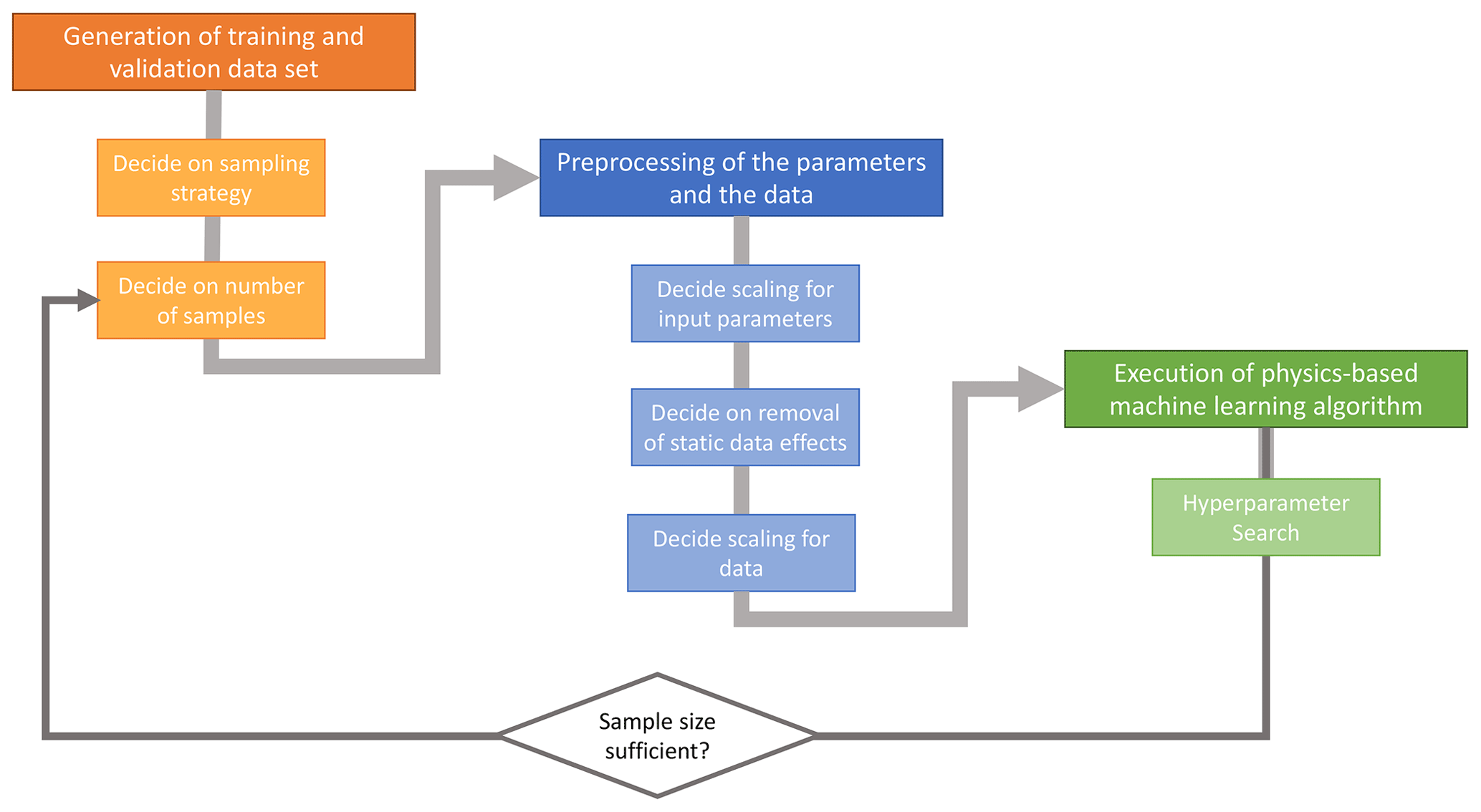
Figure 4 Schematic representation of the workflow to efficiently generate surrogate models by using physics-based machine learning techniques.

3.2 Geothermal example

For the geothermal benchmark study, we consider a three-dimensional model with three equally spaced horizontal layers (Fig. 5). The problem is nondimensional, with an extent of 1 in the x, y, and z direction. The spatial mesh is a tetrahedral mesh with 11 269 nodes.

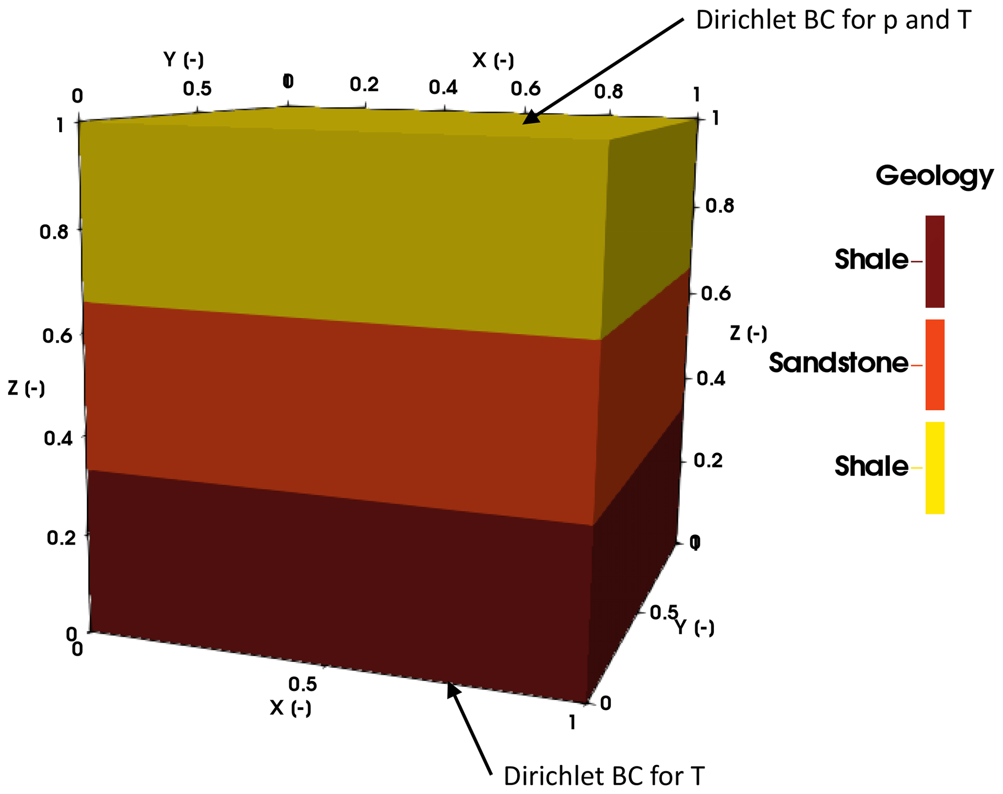
Figure 5 Representation of the geological model used for the geothermal benchmark study. In addition to the geological layers the boundary conditions are also indicated.

As the physical model, we take a fully coupled hydrothermal simulation into account, for which we consider the heat transfer equation (Nield and Bejan, 2017):

$$\begin{array}{}\text{(3)}& \begin{array}{rlrl}& {\displaystyle \frac{\partial \left({\left(\mathit{\rho }c\right)}_{\mathrm{m}}T\right)}{\partial t}}& & =\mathrm{\nabla }\cdot \left(\mathit{\lambda }\mathrm{\nabla }T-{\left(\mathit{\rho }cT\right)}_{\mathrm{f}}v\right)+H,\\ & \text{with}{\left(\mathit{\rho }c\right)}_{\mathrm{m}}& & =\left(\mathrm{1}-\mathit{\varphi }\right){\mathit{\rho }}_{\mathrm{s}}{c}_{\mathrm{s}}+\mathit{\varphi }{\mathit{\rho }}_{\mathrm{f}}{c}_{\mathrm{f}},\\ & \text{and}{\mathit{\lambda }}_{\mathrm{m}}& & =\left(\mathrm{1}-\mathit{\varphi }\right){\mathit{\lambda }}_{\mathrm{s}}+\mathit{\varphi }{\mathit{\lambda }}_{\mathrm{f}}.\end{array}\end{array}$$

Here, ρ is the density, c the specific heat capacity, T the temperature, t the time, λ the thermal conductivity, H the radiogenic heat production, and ϕ the porosity. The subscripts m, s, and f stand for the porous medium, the solid properties, and the fluid properties, respectively. For the fluid discharge v, we consider Darcy's law (Nield and Bejan, 2017):

$$\begin{array}{}\text{(4)}& v=-{\displaystyle \frac{k}{\mathit{\mu }}}\left(\mathrm{\nabla }p+{\mathit{\rho }}_{\mathrm{f}}g\mathrm{\nabla }z\right),\end{array}$$

where k denotes the permeability, μ the viscosity, p the pressure, g the gravity acceleration, and z the vertical coordinate component. In this section, we consider natural convection resulting in a temperature-dependent density of the following form (Nield and Bejan, 2017):

$$\begin{array}{}\text{(5)}& {\mathit{\rho }}_{\mathrm{f}}={\mathit{\rho }}_{\mathrm{ref}}\left(\mathrm{1}-\mathit{\alpha }\left(T-T_{\mathrm{ref}}\right)\right),\end{array}$$

where the subscript ref denotes the reference properties and α the thermal expansion coefficient. Furthermore, we consider the Boussinesq assumption (Nield and Bejan, 2017):

$$\begin{array}{}\text{(6)}& B=\mathit{\alpha }\mathrm{\Delta }T.\end{array}$$

Note that we consider the nondimensional representation to investigate the relative importance of the material properties and to improve the efficiency. This means all properties and variables in the following are presented in their dimensionless form. Since nondimensionalization is not the focus of this paper, we only present the nondimensional equations themselves and not their derivations. For a detailed derivation of the nondimensional equations refer to Degen (2020) and Huang (2018). The nondimensional heat and fluid flow can be expressed as

$$\begin{array}{}\text{(7)}& \begin{array}{rl}{\displaystyle }\mathrm{\nabla }\cdot q^{*}& {\displaystyle }=\mathrm{0},\\ {\displaystyle }{q}^{*}& {\displaystyle }=-{\mathrm{\nabla }}^{*}{p}^{*}+\sqrt{\mathit{Ra}}{T}^{*}\widehat{\mathit{j}},\\ {\displaystyle \frac{\partial T^{*}}{\partial t}}+\sqrt{\mathit{Ra}}{q}^{*}\cdot {\mathrm{\nabla }}^{*}{T}^{*}-{\mathrm{\nabla }}^{\mathrm{2}}{T}^{*}& {\displaystyle }=\mathrm{0},\\ {\displaystyle }\text{with}\mathit{Ra}& {\displaystyle }={\displaystyle \frac{{\mathit{\rho }}_{\mathrm{ref}}g\mathit{\alpha }k{l}_{\text{ref}}\mathrm{\Delta }T}{\mathit{\mu }\mathit{\kappa }}},\\ {\displaystyle }\text{and}\mathit{\kappa }& {\displaystyle }={\displaystyle \frac{{\mathit{\lambda }}_m}{{\mathit{\rho }}_{\mathrm{ref}}{c}_f}}.\end{array}\end{array}$$

Here, the asterisk denotes the nondimensional variables, $\widehat{\mathit{j}}$ the unit vector, and l_ref the reference length.

For the numerical modeling, we use the finite-element software DwarfElephant (Degen et al., 2020a, b), which is based on the MOOSE framework (Permann et al., 2020).

The pressure distribution has a Dirichlet boundary condition of zero at the top and the remaining boundary conditions are no-flow boundaries. For the temperature, we apply Dirichlet boundary conditions at the top and the base of the model, where the top boundary condition has a value of zero and the base one has a value of 1. The remaining boundaries have zero Neumann boundary conditions. For the time stepping, we consider an equal spacing between 0 and 0.8, resulting in 15 time steps. Note that the time is dimensionless. The initial condition is zero everywhere in the model domain.

During the study, we assume that the top and base layers are low-permeability layers with a variation range of 1 to 4 for the Rayleigh number (Ra) and the middle layer is a highly permeable layer with a variation range of 36 to 64 for Ra. For these parameter ranges, we construct two training datasets: one with 50 samples and one with 100 samples. Throughout the entire paper, we use a Latin hypercube sampling strategy for the training datasets and a random sampling strategy for the validation dataset. In the case of the geothermal example, we have a validation dataset consisting of 20 samples.

For this benchmark example, we investigate how to construct reliable surrogate models for the pressure and temperature distribution resulting from the nonlinear and hyperbolic PDE (Eq. 3). We employ the non-intrusive RB method with a Gaussian process regression (GPR) as the machine learning method during the projection step since the variations tested here are linear. We use the GPR method during the projection step since it is known to perform well for linear variations and has fewer hyperparameters that need to be determined, yielding a more efficient construction of the surrogate model.

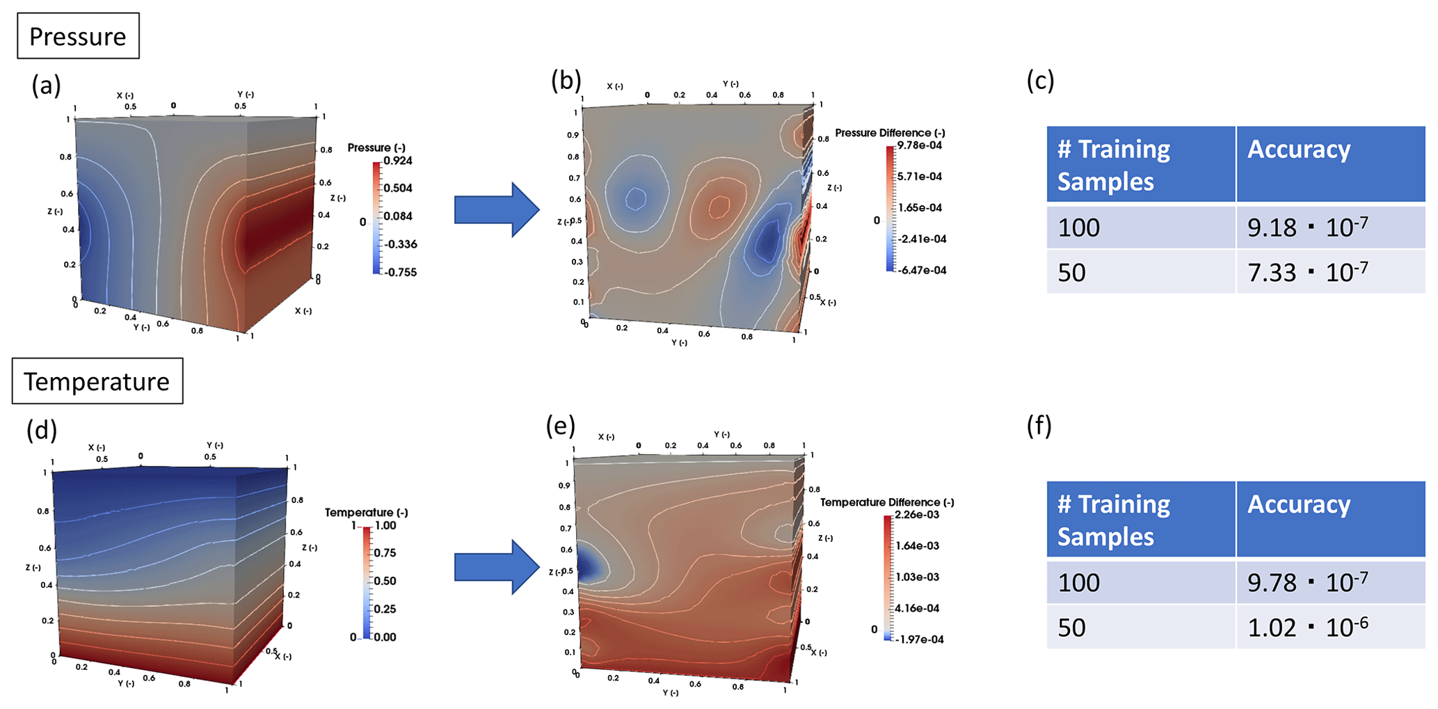
Figure 6 Representation of the accuracy for the pressure and temperature distribution of the geothermal benchmark study. The top three panels show the model for the pressure response; panel (a) contains the original pressure distribution of the finite-element model, panel (b) shows the error between the reduced and full model, and panel (c) lists the accuracy of the reduced pressure response model for different training sample sizes. Analogously, the three bottom panels display the temperature response; panel (d) shows the temperature response of the finite-element model, panel (e) illustrates the error between the reduced and full model, and panel (f) displays the accuracy of the reduced temperature response model for varying training sample sizes.

We start the discussion with the surrogate model for the pressure distribution (top three panels of Fig. 6). The pressure distribution for the full finite-element model is shown in Fig. 6a. As mentioned in the description of the non-intrusive RB method, the method consists of two steps: the POD step (where we determine the basis functions) and the projection step (where the weights are determined). Overall, we desire to achieve an accuracy of 10⁻³; this accuracy is chosen with respect to typical errors of pressure measurements. To reach this accuracy, we require five basis functions, which are partly shown in Fig. 3. The error distribution for one randomly chosen sample from the validation dataset is shown in Fig. 6b. Here, we can see that the error distributions follow the pattern of the higher-order modes obtained by the POD method. This is in accordance with our expectations since we truncated the basis after reaching the desired accuracy. Consequently, we lose information about the higher-order modes. In Fig. 6c, we compare the accuracies for the training datasets with 100 and 50 samples, and we reach our desired accuracy for 50 simulations .

Similar results are obtained for the temperature distribution (Fig. 6d), where we require seven basis functions to obtain an accuracy of 10⁻³. Note that in this example, we chose the same tolerances for the pressure and temperature model. However, they do not need to be the same. Hence, the tolerances can be adjusted to the varying measurement accuracies of, for instance, pressure and temperature measurements. Also, for the temperature model we observe that the errors (Fig. 6e) follow the distribution of the higher-order POD modes and that 50 simulations in the training set are sufficient to reach the desired tolerance (Fig. 6f).

The benefits of the method become apparent when we have a closer look at the computation times. The finite-element model requires 85 s to solve for the pressure and temperature for all time steps. On the other hand, the reduced model requires 1 ms for solving either the pressure or the temperature for a single time step. Note that in the case of the reduced model, we can solve for individual time steps and state variables and do not need to solve for the entire time period if we are, for instance, only interested in the final time step. But even if we want to solve for both variables for all time steps, we are nearly 3 orders of magnitude faster with the reduced model. From previous studies using the intrusive RB method, this speed-up is expected to be higher for real case models because the complexity of these models increases more slowly than the degrees of freedom (Degen et al., 2020a; Degen and Cacace, 2021; Degen et al., 2021b).

3.3 Geodynamic example

For the numerical modeling of the geodynamic benchmark, we use the thermomechanical finite-element code SULEC v. 6.1 (Buiter and Ellis, 2012; Ellis et al., 2011; Naliboff et al., 2017). The software solves the conservation of momentum,

$$\begin{array}{}\text{(8)}& \mathrm{\nabla }\cdot {\mathit{\sigma }}^{\prime }-\mathrm{\nabla }p+\mathit{\rho }g=\mathrm{0},\end{array}$$

and the incompressible continuity equation,

$$\begin{array}{}\text{(9)}& \mathrm{\nabla }\cdot v=\mathrm{0},\end{array}$$

where σ^′ is the deviatoric stress tensor, p is the pressure, ρ is the density, g is the gravitational acceleration, and v is the velocity. The density variations are described analogous to the geothermal example (Eq. 5). Also, the heat transfer is similar to the geothermal description (Eq. 3), with the main difference that we obtain shear heating as an additional source term:

$$\begin{array}{}\text{(10)}& \mathit{\rho }c\left({\displaystyle \frac{\partial T}{\partial t}}+v\cdot \mathrm{\nabla }T\right)=\mathrm{\nabla }\cdot \mathit{\lambda }\mathrm{\nabla }T+H+\mathrm{2}{\mathit{\sigma }}_{\mathrm{2}}^{\prime }\cdot {\dot{\mathit{\epsilon }}}_{\mathrm{2}}^{\prime }.\end{array}$$

Here, ${\mathit{\sigma }}_{\mathrm{2}}^{\prime }$ and ${\dot{\mathit{\epsilon }}}_{\mathrm{2}}^{\prime }$ are the second invariant of the deviatoric stress and strain tensors, respectively.

For this study, we consider the development of a salt dome (Fig. 7). The linear viscous salt rises buoyantly upward through linear viscous sediment layers. The rise is initiated by a sinusoidal perturbation of the salt–sediment interface with a 40 m amplitude. Note that all Neumann boundary conditions (Fig. 7) are no-flow boundary conditions. All velocity Dirichlet boundary conditions have a value of 0 m s⁻¹. Furthermore, the temperature at the top of the model has a fixed value of 0 ^∘C and at the base a value of 140 ^∘C. The discharge temperature Dirichlet boundary condition at the lateral sides has a value of 0 m³ s⁻¹. The model extends 8 km in the x direction and 4 km in the y direction. For the spatial discretization of the 2D benchmark study, we use quadratic cells with a resolution of 40 m × 40 m, resulting in a structured mesh with 20 301 nodes. SULEC solves for velocities on the nodes, whereas pressure is constant over the cells and obtained in Uzawa iterations (Pelletier et al., 1989).

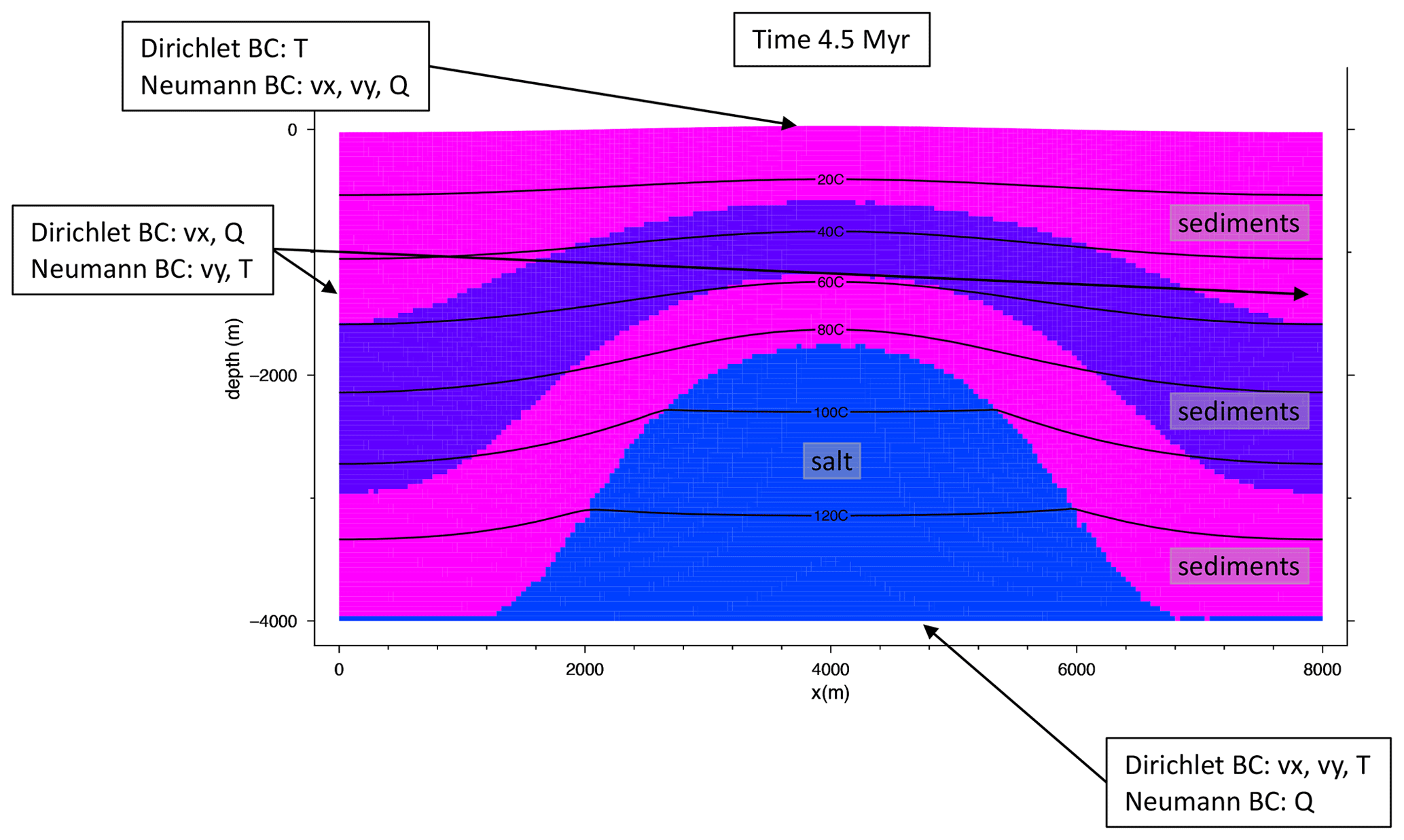
Figure 7 Geological model of the salt diapir at 4.5 Myr. The temperature isolines are plotted for a realization from the training dataset.

For the time stepping, we use fixed time steps of 5 kyr and simulated from 0 to 6.25 Ma. In contrast to the previous example, we consider the dimensional case here. Nondimensional forward simulations are more efficient for physics-based machine learning methods. However, many simulations in the field of geosciences are often conducted in dimensional form. Hence, we want to illustrate how these simulations need to be processed to ensure an efficient construction of the surrogate models. Note that we describe the general workflow in Sect. 3.1; we will only briefly highlight the most important steps for the geodynamic case study here.

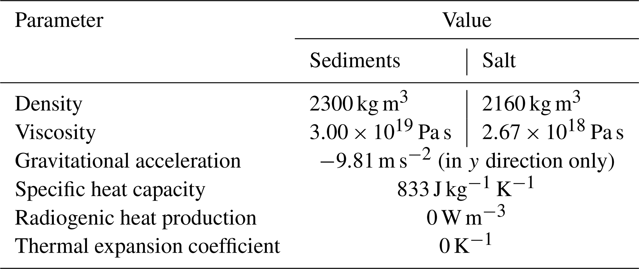
For the given example, we allow a variation of the thermal conductivity of the sediments between 2.5 and 3.0 W m⁻¹ K⁻¹ and for the salt between 5.0 and 8.0 W m⁻¹ K⁻¹. This means we assume that the thermal conductivity of the salt has higher uncertainty than that of the sediments. We construct a training set of 50 samples with a Latin hypercube sampling strategy, and the validation dataset consists of 10 randomly chosen samples. The remaining model parameters stay constant throughout all simulations and are displayed in Table 2. We consider linear viscous materials that are tracked with tracers. For the benchmark example, we have in total 182 709 tracers at the start, yielding a minimum of 16 and a maximum of 20 tracers per cell (which are maintained by a tracer population control). The tracers are moved using a second-order Runge–Kutta scheme.

Table 2 Model parameters of the geodynamic benchmark example.

In Fig. 8, we present the result of the finite-element forward model and the accuracy of the surrogate model. Figure 8a shows the temperature distribution of the full model ranging from 0 to 140^∘C. We observe that the changes induced by the variations of the thermal conductivities (at the interface between the salt dome and the sediments) are much smaller than the initial temperature distribution. Furthermore, the initial temperature distribution is independent of any variations in the thermal conductivity. Hence it is the same for all forward simulations. Therefore, we train the model only on the temperature variations, which we additionally scale between 0 and 1 by calculating the minimum and maximum temperature values of the entire training dataset. The scaled temperature distribution used within the algorithm is shown in Fig. 8b. If visualizations of the absolute temperature distribution are desired they are obtained by adding the initial condition after calculating the reduced forward model.

Figure 8c displays the difference between the full and reduced model, where the highest errors are of the order of 0.1 ^∘C. This means that the errors induced by the approximation are lower than those of typical temperature measurements. We observe the highest errors at the flanks, in the lower part of the model. This matches our expectations since we have the largest changes at the interface between the salt diapir and the surrounding sediments. Furthermore, the temperature distribution at the flanks is more diffusive in contrast to the very sharp changes at the top of the salt dome, which adds to the higher errors of the reduced model at these locations. In total, we required 18 basis functions to reach the given accuracy. Note that the number of basis functions is relatively high because of the rather abrupt changes that we need to capture.

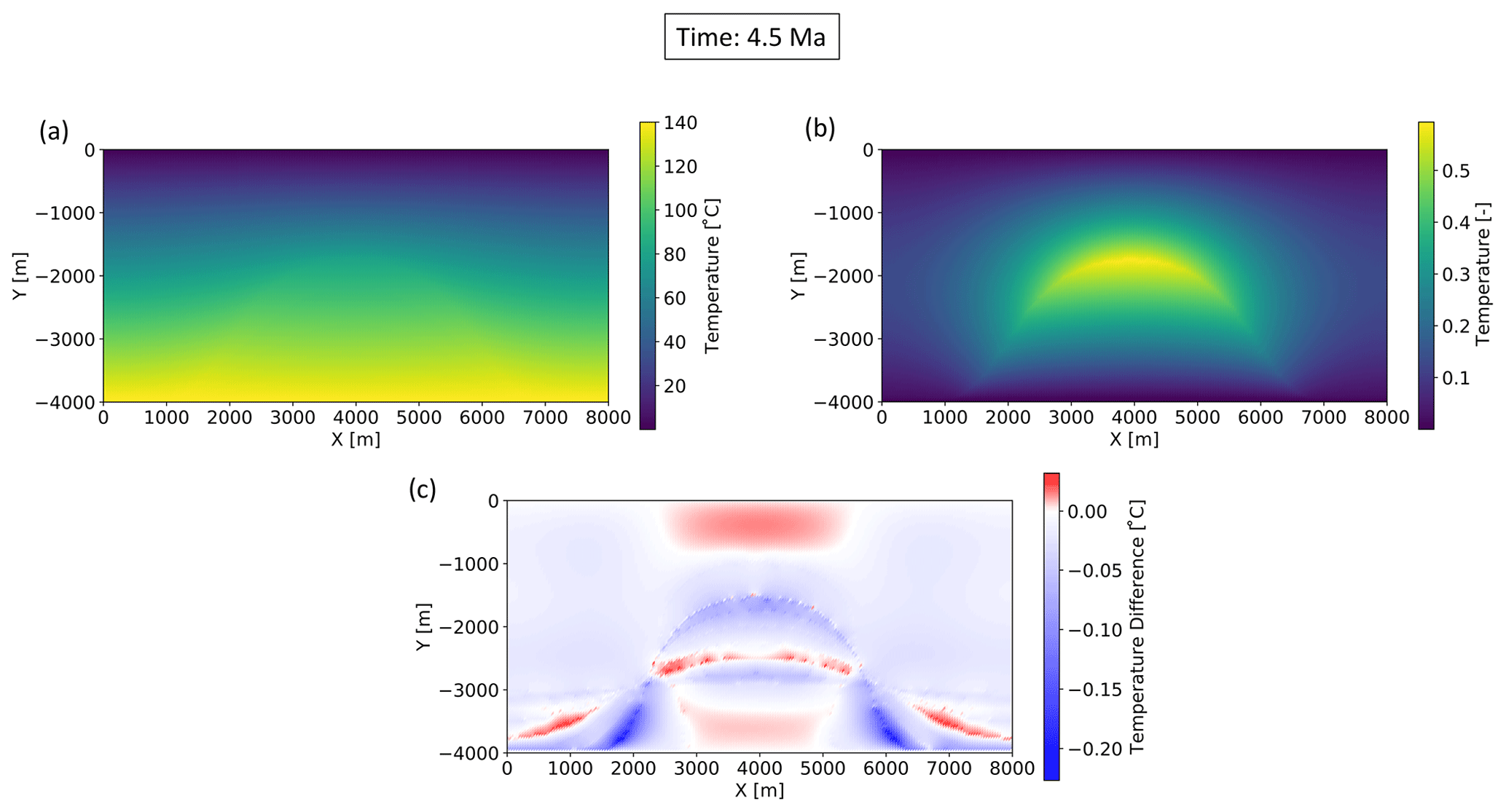
Figure 8 Comparison of the full finite-element and the reduced model. (a) The temperature distribution of the finite-element solution, (b) the scaled finite-element solution as utilized in the training of the reduced model, and (c) the difference between the reduced and full solution.

Analogously to the geothermal example, we evaluate the gain in computation time. The average computation time over 50 finite-element simulations is 1.05 h (including input–output processes) on two Intel Xeon Platinum 8160 CPUs (24 cores, 2.1 GHz, 192 GB of RAM) using the PARallel DIrect SOlver (PARDISO) (Schenk and Gärtner, 2004). In contrast, the average computation time over 50 reduced simulations is about 2 ms for a single time step. Note that with the reduced model, we can perform predictions for individual time steps. That this is of general interest can be seen directly in this case study. Although we calculate the solution for all 1250 time steps, we output 14 only. Note that only these 14 time steps have been used to construct the surrogate model. However, the model is trained for spatial and temporal variations. Hence, we can also retrieve intermediate time steps. The obtained speed-ups range between 5 orders of magnitude (interested in all 14 display time steps) and 6 orders of magnitude (interested in a single time step).

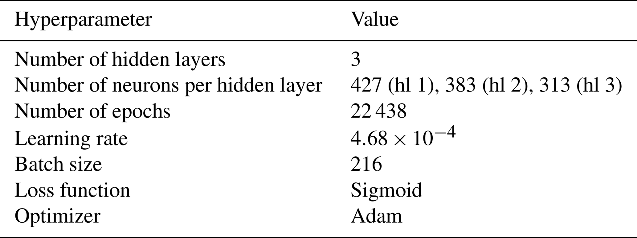
Table 3 Hyperparameters of the neural network for the geodynamic benchmark example. Note that hl denotes hidden layers.

To construct the surrogate model, we require in total 18 basis functions to reach our POD tolerance of 10⁻³, as displayed in Fig. 9. Having a closer look at the basis functions, we observe that the “low-frequency” information is presented in the first basis functions and the “high-frequency” information in the last basis functions. This nicely shows the analogy between the non-intrusive RB method and the Fourier decomposition.

For the determination of the hyperparameters, we use Bayesian optimization with hyperbands (as described in Sect. 3.1). To save memory, the training was performed using only every second node. All results and accuracies presented here are calculated using all nodes in space. The hyperparameters obtained after optimization are presented in Table 3. With these hyperparameters, we obtain an error of $\mathrm{2.21}\times {\mathrm{10}}^{-\mathrm{6}}$ for the scaled training dataset and an error of $\mathrm{1.99}\times {\mathrm{10}}^{-\mathrm{6}}$ for the scaled validation dataset.

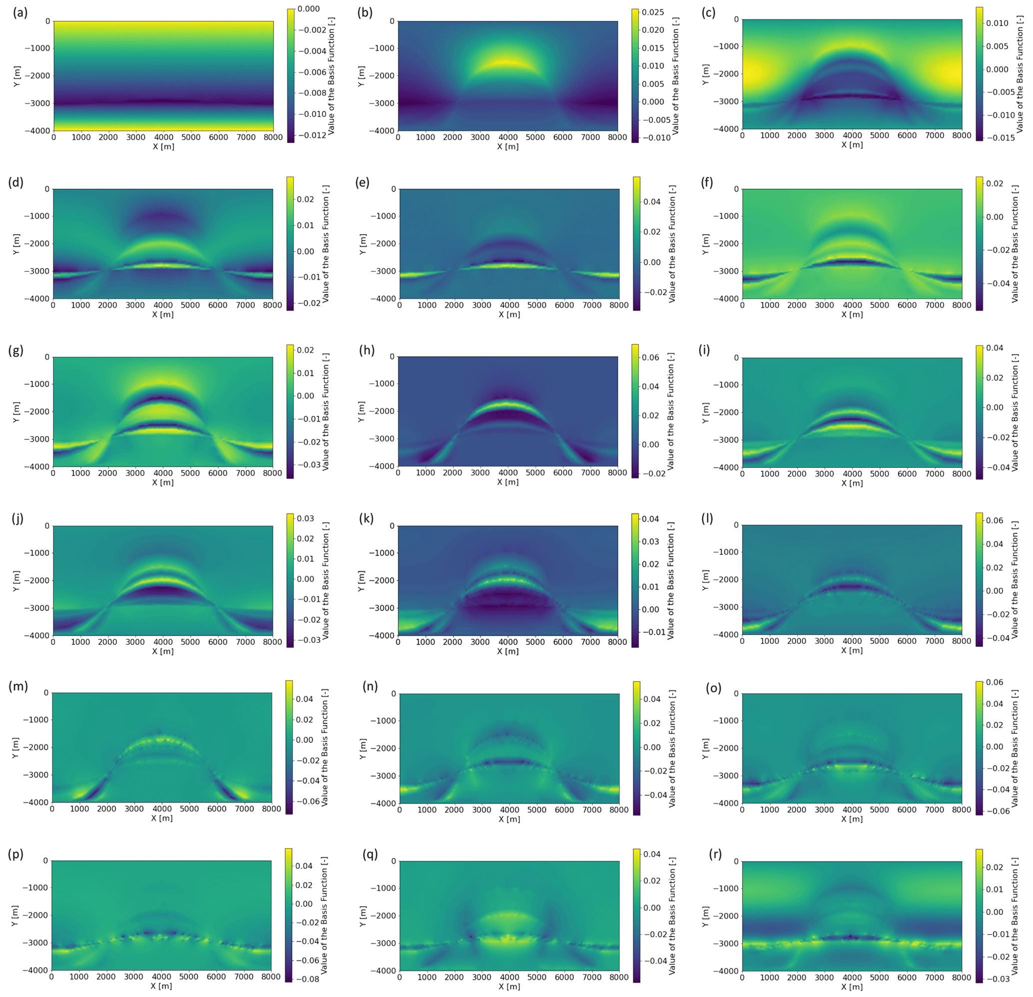
Figure 9 Illustration of the 18 basis functions of the surrogate model, where (a) shows the first basis function and (r) the last basis function.

3.4 Hydrological example

In this section, we present a proof-of-concept hydrological application inspired by a well-known two-dimensional infiltration problem on a domain with soil heterogeneity, originally proposed by Forsyth et al. (1995). The setup is illustrated in Fig. 10. The domain has impervious lateral and bottom boundaries and four zones with different soils, represented through different permeabilities. A uniform initial pressure of $h=-\mathrm{100}$ cm was set and an infiltration flux q is prescribed on the top left corner of the domain.

Although this is evidently a benchmark problem, it offers many of the complexities which arise in subsurface flow simulation, such as heterogeneity and sharp infiltration fronts, and therefore nicely serves as a proof of concept.

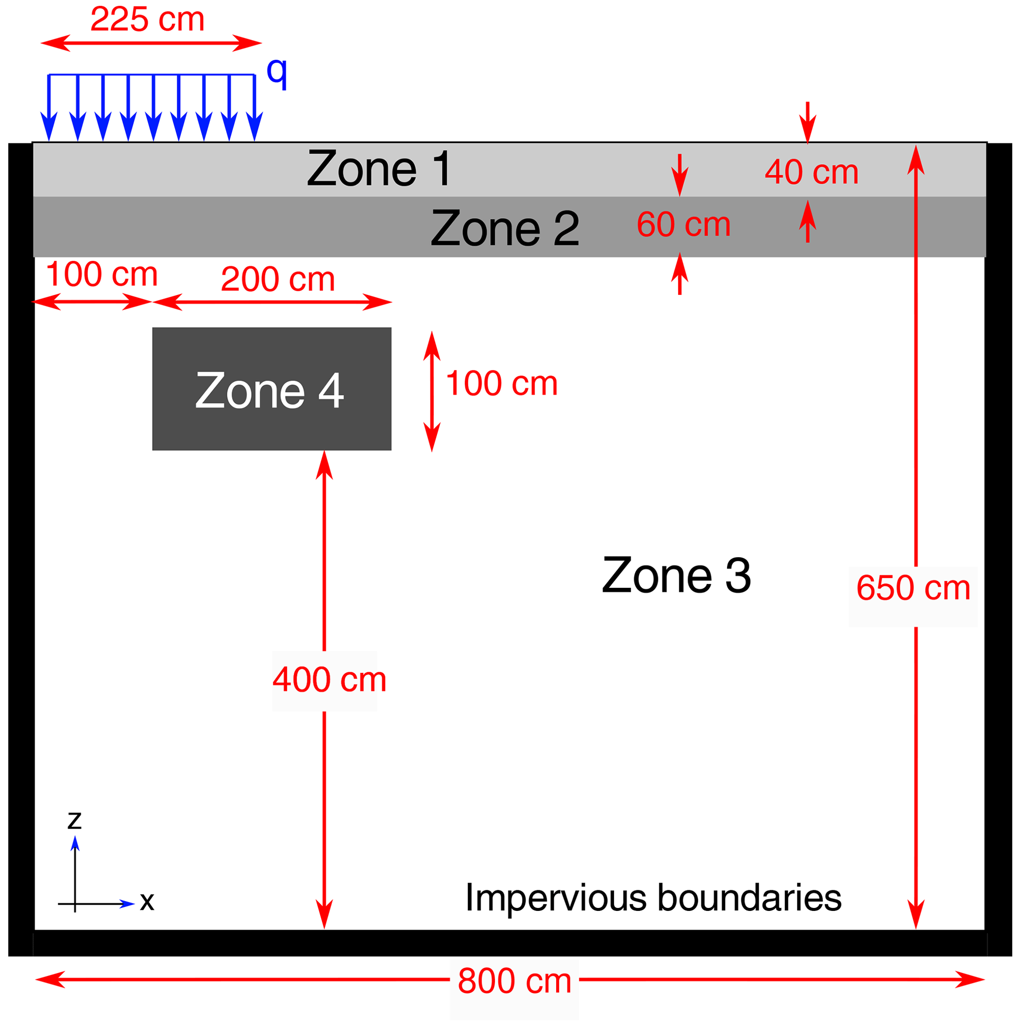
Figure 10 Sketch of the infiltration problem for the proof-of-concept hydrological application. Adapted from Forsyth et al. (1995).

The physical model for variably saturated flow in a porous medium is the Richards equation (Richards, 1931):

$$\begin{array}{}\text{(11)}& {\displaystyle \frac{\partial \mathit{\theta }}{\partial t}}=\mathrm{\nabla }\left[\mathbf{K}\left(h\right)\mathrm{\nabla }\left(h+z\right)\right],\end{array}$$

where h is pressure, θ is the volumetric soil water content, K is hydraulic conductivity, t is the time, and z is the vertical coordinate. A soil model is necessary to provide closure relationships, for which, for this case, we use the Mualem model for the water retention curve θ(h) and the van Genuchten model for K(θ(h)) (van Genuchten, 1980). The resulting mathematical model is a highly nonlinear diffusion equation, formally an elliptic–parabolic PDE, which also shows very sharp front propagation akin to that of advection problems (Caviedes-Voullième et al., 2013).

To numerically solve Eq. (11) we rely on the well-established hydrological model ParFlow (Kuffour et al., 2020). ParFlow solves the Richards equation via a backward Euler finite-difference scheme and uses multigrid-preconditioned Newton–Krylov methods to solve the resulting system. It is massively parallelized and, in fact, recently ported to GPUs (Hokkanen et al., 2021). For the infiltration problem here, we do not leverage ParFlow's HPC capabilities, since the time to solution of this problem is only a few seconds on a single CPU core. In contrast, we ran all realizations of both training sets in parallel in an HPC node in the JUWELS system at the Jülich Supercomputing Centre.

In this proof-of-concept exercise, we first construct a training set for the non-intrusive RB method. A total of 100 different combinations of permeabilities for the four materials in the domain are considered, as well as various inflow rates q. A Latin hypercube strategy was used for sampling the five-dimensional parameter space. A validation set of 20 samples (with a random sampling strategy) was also generated. Importantly, permeability values follow a lognormal distribution, whereas the infiltration flux follows a uniform distribution. The original permeabilities proposed by Forsyth et al. (1995) were selected as the mean value for the lognormal distributions with a standard deviation of 1. The uniform distribution for the infiltration flux was centered around 4 cm d⁻¹ and a standard deviation of 0.5.

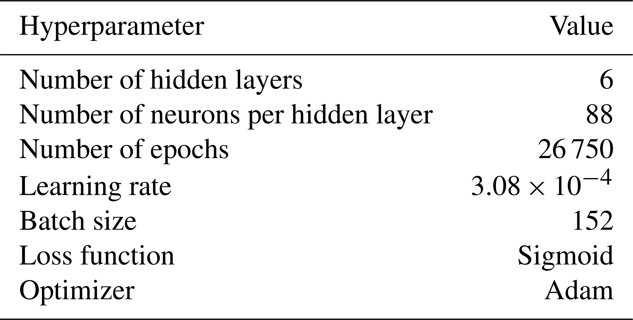
Similar to the previous case studies, we use the non-intrusive RB method to construct a surrogate model that predicts the hydraulic head for every parameter combination in the above-defined ranges at every time step. For the construction of the surrogate model, we require 124 basis functions. This number is significantly larger than in the previous examples. This is related to the more pronounced nonlinearity of the solutions, which differs for the various time periods. Nonetheless, we obtain solutions in less than 3 ms (calculated over 100 iterations), yielding a speed-up of 3 orders of magnitude (if we want to predict the solution for a single time step). With the hyperparameters presented in Table 4, we achieve an accuracy of $\mathrm{8.71}\times {\mathrm{10}}^{-\mathrm{7}}$ for the scaled training set and $\mathrm{2.89}\cdot {\mathrm{10}}^{-\mathrm{5}}$ for the validation dataset.

Table 4 Hyperparameters of the neural network for the hydrological benchmark example. Note that hl denotes hidden layers.

The errors for the training and validation dataset are global errors. In the next step, we look at the spatial distribution of the approximation errors. Therefore, we pick an arbitrary solution from the validation dataset and compare the solution for the last time step (Fig. 11). Figure 11a and b look visually the same, which is the reason we focus the presentation on the difference plot displayed in Fig. 11c. Here, we observe that no part of the model is underrepresented and that the errors are the highest in areas where there is strong spatial heterogeneity of the permeability fields and of the infiltration flux (most notably around zone 4), both of which contribute to strong nonlinear gradients in hydraulic head. The magnitude of the differences is below 2 cm, which for all practical purposes is excellent agreement.

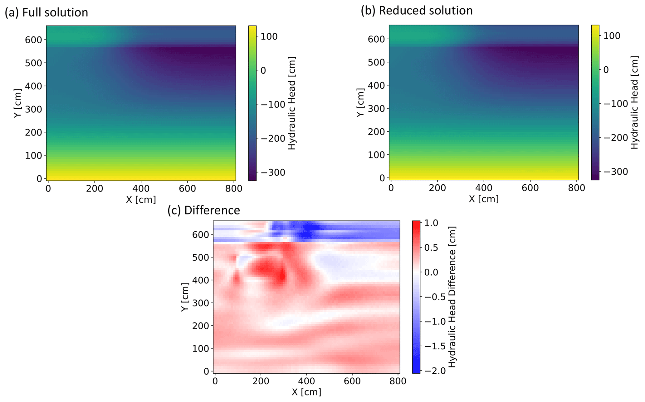
Figure 11 Comparison of the prediction accuracy of the surrogate model for subsurface hydrology. We show in (a) the full solution of the Richards equation, in (b) the prediction from the surrogate model, and in (c) the difference between the full and reduced solutions for the time step 30 of an arbitrarily chosen solution from the validation dataset.

To ensure that the behavior is the same over the entire time period, we pick four random time steps and repeat the procedure (Fig. 12). Note that for an easier comparison between the various temporal responses, we plot the solution over the number of nodes and no longer in the 2D representation from above. We observe that the approximation quality is good over the entire time period and that the errors tend to decrease with progressing time steps, which is again related to the nonlinearity.

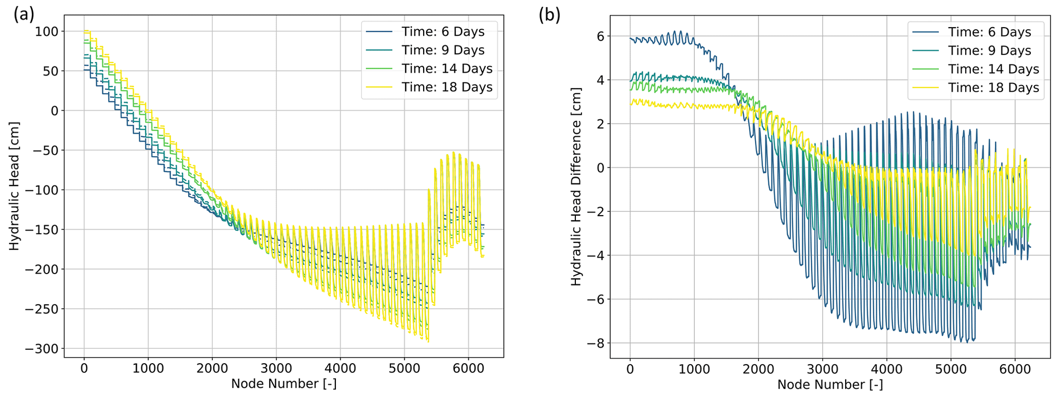
Figure 12 Comparison of the prediction accuracy of the surrogate model for various time steps. We show in (a) the response and in (b) the differences between the full and reduced solutions. In panel (a) the full solutions are denoted by solid lines and the reduced solutions by dashed lines.

3.5 Physics-based machine learning versus data-driven machine learning

In the previous section, we demonstrated how the non-intrusive RB method can be used to construct reliable and efficient surrogate models through three designated benchmark examples. The focus of this paper is to illustrate the perspective of physics-based machine learning for subsurface geoscientific applications and how this perspective might differ for various approaches existing for physics-based machine learning. Therefore, we extend the previous sections by constructing surrogate models through neural networks for all three examples. We chose neural networks for this purpose because this enables a comparison between a physics-based and a data-driven machine learning approach, while at the same time also showing the differences between the two paradigms presented for physics-based machine learning, as we detail later on.

One advantage associated with physics-based machine learning vs. data-driven approaches is the reduction in the amount of training data required by reducing the number of admissible solutions through physical knowledge (Faroughi et al., 2022; Raissi et al., 2019). Due to the simplicity of the presented examples this could not be observed, and we obtained similar global errors for both the non-intrusive RB and the NN surrogate models. Nonetheless, it has been shown in, for instance, Santoso et al. (2022) that for more complex applications significantly fewer data are required for physics-based approaches.

Another important aspect becomes apparent by focusing on the local error distributions presented in Fig. 13. Generally, the error distributions show a noisy behavior for the data-driven approach, whereas they exhibit a smooth behavior for the non-intrusive RB method. Furthermore, we can observe in the areas marked with A and B that boundary conditions are not preserved. Not only are they not preserved but also show one of the highest errors in the entire surrogate model, which is related to the general challenge of optimizing for loss function values close to zero (Chuang and Barba, 2022). Furthermore, we observe a sharp line in area C, where regions of higher and lower error values occur adjacent to each other, which can not be explained through physical processes. Similar observations of error distributions not corresponding to physical effects are observed for areas D and E. In contrast, the error behavior of the non-intrusive RB method is clearly related to physical processes and changes in material properties, as detailed in the previous sections. This observation is not only relevant for the comparison of data-driven and physics-based machine learning approaches but also for distinguishing between the various physics-based machine learning methods. Methods that use physics-guided loss functions (e.g., PINNs) will exhibit the same error behavior as the physics only enter in the loss functions, and physics-guided architecture will also suffer from this as long as the outer layer still operates as a neural network.

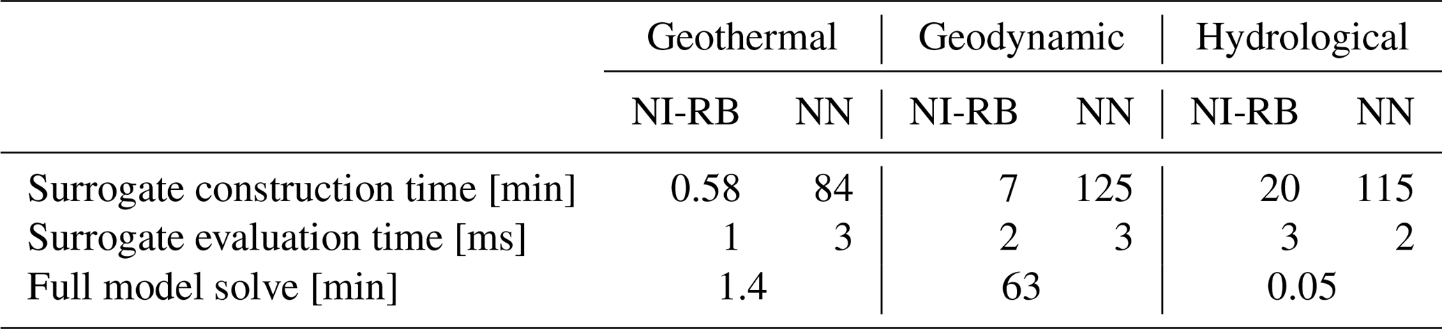
Finally, in Table 5, we compare the construction times for the surrogate models (for both the non-intrusive RB method and the NN), the evaluation times for a single surrogate model run, and the original computation times for the full-dimensional simulations. The first observation is that the construction time of the surrogate models is considerably smaller for the non-intrusive RB method than for the NN. This is related to the dimension of the training dataset entering the machine learning part. For the non-intrusive RB method, we first determine the basis functions and determine only the coefficient over the machine learning technique. This means that the training data have the dimension N_s×N_bfs, where N_s is the number of snapshots and N_bfs is the number of basis functions. In contrast, the dimension of the training dataset for the NN is N_s×N_dofs, where N_dofs denotes the number of spatial degrees of freedom (e.g., nodes, elements). Typically the number of basis functions is orders of magnitude smaller than the degrees of freedom, yielding a reduction in the construction time. The evaluation cost of the surrogate models is comparable for both the non-intrusive RB method and the NN. Furthermore, the evaluation times of the surrogate model are between 3 and 6 orders of magnitude lower than the full-order evaluations. This demonstrates the benefits of surrogate models for applications where either results are required in real time or numerous evaluations are necessary. Note that again the discussed aspect of the increased construction time applies not only to NNs but also to methods such as PINNs.

To conclude, even in applications where we do not have the added benefit of the reduction in the amount of simulation required, the non-intrusive RB method performs better than data-driven alternatives, while yielding a lower computational cost.

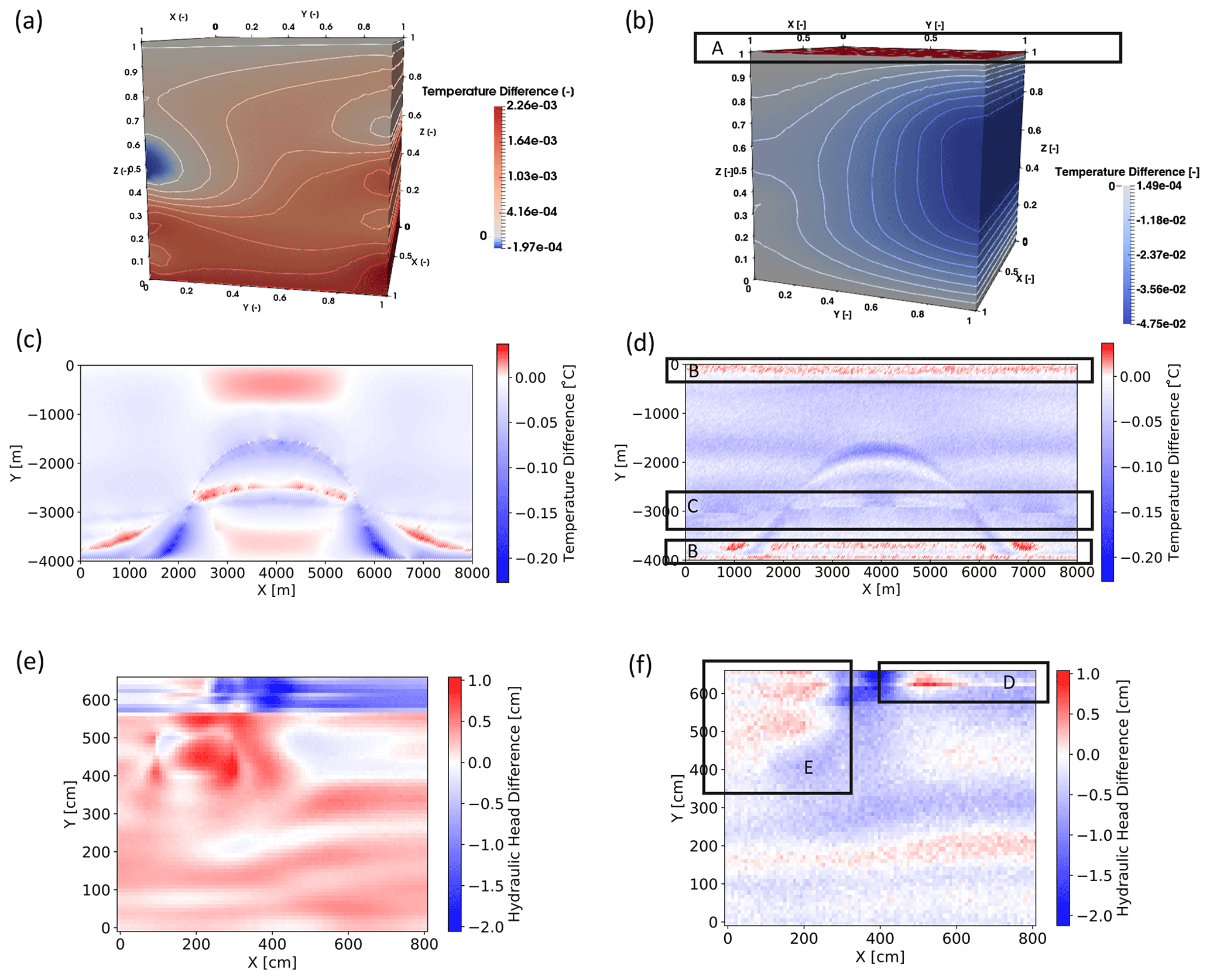
Figure 13 Comparison of the local error distribution for the surrogate models of the geothermal example (a) non-intrusive RB method and (b) NN, the geodynamic example (c) non-intrusive RB method and (d) NN, and the hydrological example (e) non-intrusive RB method and (f) NN.

Table 5 Comparison of the computational cost for the three benchmark examples considering both physics-based and data-driven machine learning methods. Note that the construction time excludes the time required for the generation of the training data. The hyperparameters of the NN are identical to the ones described for the non-intrusive RB method. For the geothermal example, we use the hyperparameters provided for the geodynamic example since the non-intrusive RB method used a Gaussian process regression, and we perform the construction only for the temperature.

Another point to note is that in this paper we looked at parameterized partial differential equations, assuming the parameter of interest is a material parameter. This assumption is purely exemplary. PINNs sampling the input from the state itself can incorporate changing initial and boundary conditions through the sampling. Similar considerations are valid for the non-intrusive RB method. Here, additional parameters are included to take variations in the initial and boundary conditions into account. Examples are provided in, for instance, Degen (2020), Degen and Cacace (2021), Degen et al. (2022b), and Grepl (2005).

4 Challenges and requirements

We introduced three challenges and four requirements common to many geoscientific applications in the Introduction. In the following, we elaborate on how physics-based machine learning, in particular the non-intrusive RB method, can help to address these challenges and fulfill the requirements.

4.1 Challenge 1: sensitivity analysis

Global sensitivity analyses determine the relevant physical parameters for the respective processes and their correlation (Sobol, 2001). Therefore, they enhance our understanding of the subsurface but are computationally demanding, making them prohibitive for large-scale models. The non-intrusive RB method addresses this computational challenge through the construction of surrogate models. As pointed out by Razavi et al. (2012) and Song et al. (2015) the usage of surrogate models in sensitivity analyses is critical. It is critical because if the surrogate model does not represent the high-dimensional model appropriately, we face the high risk of producing biased sensitivity analyses and deriving the wrong conclusions. Although we agree with this statement, we think it is useful to distinguish between different surrogate modeling techniques highlighting the importance of a surrogate model fulfilling the four listed requirements. As shown for its intrusive counterpart, the results of a sensitivity analysis do not change significantly with the surrogate model accuracy (Degen and Cacace, 2021).

The non-intrusive RB method maintains the input–output relationship of the PDEs, in contrast to, for instance, PINNs. This means that in the classical formulation PINNs sample from spaces in time and space and produce as output state information at any arbitrary location of the model. These considerations are for a fixed set of model parameters (e.g., material properties), making the method unsuitable for sensitivity analysis, where the model parameters need to be changed. This is a disadvantage not only of PINNs but also of all other methods that follow the idea of going from state information to state information, while maintaining the same material properties. Note that recent developments (Zhang et al., 2022) allow a variation of the material properties. However, the disadvantage is that the material properties embedded in the loss function change throughout the training process, meaning that an unphysical correlation between hyperparameters and physical parameters is introduced.

In contrast, the non-intrusive RB method yields surrogates that do not change the general characteristics of the original problem. Consequently, we can address the challenge of performing computationally expensive global sensitivity analysis by using surrogate models constructed by the non-intrusive RB method. This reduces the computational cost by several orders of magnitude, making it a suitable technique to also ensure the feasibility of global sensitivity studies for large-scale models (Degen et al., 2021b; Degen and Cacace, 2021; Degen et al., 2021a, 2022b).

4.2 Challenge 2: uncertainty

Another application field where the non-intrusive RB method offers great potential is the field of uncertainty quantification. Here, the method can be used to generate fast surrogate models as a replacement for the computationally expensive high-dimensional problem (Degen et al., 2021b, 2022c, a). Uncertainty quantification (Iglesias and Stuart, 2014) determines the uncertainties of the input parameters and has great potential in reducing the risk associated with installations. Uncertainties can be further reduced by finding the optimal position of new measurement locations by employing optimal experimental design methods (Alexanderian, 2021). Also, for this technique, the non-intrusive RB method is suitable to construct surrogate models as shown in Degen et al. (2022a). An important consideration in the usage of surrogate models for uncertainty quantification is the reliability of the surrogate. The surrogate needs to be representative of the original high-dimensional model because otherwise the uncertainty quantification is biased, analog to the discussion in the previous section. Therefore, we require at least error estimators for the surrogate model and in the ideal case error bounds, i.e., guarantees of the model accuracy. In contrast to other surrogate modeling techniques, the non-intrusive RB method further has the advantage of preserving the input–output relationship and therefore maintains the structure of the original model.

Adaptive MCMC approaches are also interesting, where a smaller reduced basis is constructed which is adapted during the MCMC analysis. The idea of constructing an adaptable reduced basis is presented in Qian et al. (2017), where the authors create a reduced basis that is valid for a trust region. An adaptive MCMC algorithm for MT applications has been presented in Manassero et al. (2020), which follows up on the ideas of Ortega-Gelabert et al. (2020).

To conclude, as for the sensitivity analyses the computational challenge is addressed by using surrogate models. Note that as before methods that map from model parameters to state information are more suitable within an uncertainty quantification framework.

4.3 Challenge 3: real time

In many geoscientific applications, we need to obtain results in real time. Examples are forecasting applications often employed in the fields of hydrology and climate (Bauer et al., 2021; Sabeena and Reddy, 2017), as well as monitoring and/or risk analyses (Asante-Duah, 2021; Kumar et al., 2021; Yu et al., 2018). The latter analysis is often important for fields such as geothermal energy and natural hazards (Kumar et al., 2021; Liu and Ramirez, 2017; Yu et al., 2018). In the field of geothermal energy that concerns the topic of induced seismicity, there is a need to have fast and reliable predictions to employ necessary security measures. However, with increasingly complex models that require more and more computation time, this leads to major challenges. In order to address these challenges, a possibility might be to think of employing physically simplified models, which could result in additional error sources that might bias further analyses. Another possibility is to employ data-driven approaches; however, how the quality of these models can be guaranteed is an open research question (Baker et al., 2019; Willcox et al., 2021). Therefore, physics-based machine learning techniques, such as the non-intrusive RB method that fulfill the four listed requirements, have great potential since the surrogate models produced are computationally fast to compute and at the same time maintain the general characteristics of the original problem.

Consequently, the challenge of producing real-time predictions is addressable by the use of surrogate models. We generally see greater potential in methods that follow the conceptual ideas of the non-intrusive RB method since they allow for both parameter and state estimation. Nonetheless, in the context of state estimation and in situations in which some physical knowledge is available, methods that map from state-to-state information (such as PINNs) are advantageous since they allow also a direct incorporation of the measurement data. However, these are not the target applications of this paper.

Looking at all three presented challenges, we see great potential in the non-intrusive RB method, which combines physics-based and data-driven approaches. This avoids simplifications on the physical level and at the same time yields explainable, generalizable, scalable, and robust models (Willcox et al., 2021), as we will detail in the next sections.

4.4 Requirement 1.1: physical scalability

To improve our understanding of the subsurface, we often want to construct models with an increasingly higher resolution in space and time and also concerning the parameter representation. To give a few examples, in the field of geodynamics we typically aim to investigate different scales in both time and space. On the one hand, we are interested in large-scale spatial deformations related to plate tectonics; on the other hand, we want to investigate how microstructures form. For the time component, we face the same issues of being interested in seismic cycles (of the order of milliseconds) and basin dynamics (of the order of millions of years) (Bauer et al., 2021; van Zelst et al., 2022). Having a single model that crosses over all scales is computationally infeasible, even with adaptive time stepping and spatial discretization schemes. Furthermore, we need to additionally consider the complexity of the parameter space. On a larger scale, local heterogeneities are often negligible and we can use homogenization approaches (Regenauer-Lieb et al., 2013) and often simpler physical formulations. On a smaller scale, these concepts are not applicable and we need to consider the full complexity.

One way to address this problem is a multilevel approach, a concept that works independently of physics-based machine learning. However, physics-based machine learning and other surrogate modeling techniques can considerably accelerate the procedure, as we show later on. The advantages of multilevel approaches to improve convergence have been pointed out by, for instance, Bauer et al. (2021). We can, for example, combine models with different spatial and temporal resolutions, which yields faster convergences. This faster convergence is achieved by starting the solve on the coarsest level first. Once we obtain results for this level, we move to the next level which has a higher resolution. However, since we already have a good starting guess, we need significantly fewer iterations on this level in comparison to the number of iterations required if we directly solved on the finer level. Multilevel or multi-fidelity approaches not only imply different spatial and temporal resolutions but also allow for the employment of different physical descriptions (adjusted to the resolution) and different methodologies (Peherstorfer et al., 2018).

Physics-based machine learning can improve the computational time on several levels. First of all, we can provide surrogate models for the coarse levels through methods such as the non-intrusive RB method. The non-intrusive RB method performs very well in the reduction of the spatial and temporal degrees of freedom but is inefficient if the dimension of the parameter space becomes too large. However, other methods might be less efficient in the reduction of space and time but more efficient in dealing with high-dimensional parameter spaces (Benner et al., 2015). Multilevel approaches allow combining these techniques. Hence, we can employ different methodologies on each of these levels tailored to the different requirements. On the finest level, we can even employ the original full-dimensional problem.

4.5 Requirement 1.2: performance scalability

In the following, we elaborate on how physics-based machine learning approaches impact the field of HPC. Therefore, we first present the current issues we face and afterwards explain how the methods presented here help to address these aspects.

Previously, we illustrated that the complexity of the considered physical processes and their associated coupling processes are constantly increasing. This has a high impact on the computational resources since more complex scenarios yield a higher computational demand, hence often requiring HPC infrastructures. At the same time, we observe the end of the scalability laws such as Dennard scaling (Frank et al., 2001) and Moore's law (Bondyopadhyay, 1998).

A paradigm shift is underway as a consequence of this. The hardware infrastructure has been moving more and more to graphics processing units (GPUs) and is becoming more heterogeneous than before. This poses major challenges for most areas of geosciences (Bauer et al., 2021), as we can no longer rely on hardware developments to cover the required higher computational demand (end of the free-lunch era), but we need to invest in adapting the algorithms and codes themselves (Bauer et al., 2021). This is a nontrivial and potentially time-consuming process that often requires rather specialized knowledge. Moreover, the specific problems can vary greatly for the different geoscientific communities. For example, the climate community relies on very large, well-established community models. Although efforts are underway to port them to GPUs (Bauer et al., 2021), the size and complexity of the codes, and potentially even their inherent structure, make this an ambitious and costly task (Lawrence et al., 2018). Often, more than one intensive kernel may exist and the low-hanging computational hotspot to port is not obvious (Gan et al., 2020). A criticism raised by Bauer et al. (2021) is that software developments are primarily driven by scientific relevance, neglecting computer science aspects in terms of efficiency, which further complicates the transition to future HPC infrastructures. The situation is different for other geoscientific communities since they have smaller – and possibly more manageable – codes, which can therefore be more flexible adapted, or more recent codes, which may even already leverage novel technologies. In either case, porting tasks are still not trivial, but with the help of current developments to leverage GPUs, such as CUDA and OpenACC, as well as domain-specific languages (DSLs) – e.g., Kokkos (Edwards et al., 2014; Trott et al., 2021), RAJA (Beckingsale et al., 2019), Alpaka (Zenker et al., 2016), GridTools (Afanasyev et al., 2021), ClawDSL (Clement et al., 2018) – the resources and expertise required can be reduced or at least compartmentalized and better distributed in time. We can also provide cross-domain platforms such as MOOSE and Firedrake to synchronize the developments in computer and domain sciences. Moreover, it is becoming increasingly relevant to consider co-design approaches (Germann, 2021), in which domain science applications (and developers) engage with library, back-end, and even hardware developers in pointing out where significant (progressive and disruptive) advances can be made without constant adaptation from scientific applications.

Other aspects that we would like to address here are the discretization of time (Bauer et al., 2021) and how to adapt beyond the current HPC infrastructures. This includes future proofing against architectural shifts, vendors, and languages. To name one example, we require strategies to adapt to GPUs from various manufacturers (e.g., upcoming AMD and Intel GPU accelerated systems). Solutions such as CUDA are optimized for Nvidia hardware, and comparing the performance of CUDA against OpenACC (or CUDA through portability layers such as Kokkos) yields indications that this transition still poses challenges (Artigues et al., 2019; Baig et al., 2020). These considerations do not even cover the problems that might arise from tensor processing units (TPUs). Overall, the heterogeneous computing infrastructures of the future and asynchronous processes pose major and partly unpredictable challenges, emphasizing the need for flexible, open-source software projects.

There are various possibilities to address these issues. The first is naturally the intensive training of researchers in the field of HPC, including, for instance, advanced programming training sessions, which is a long learning process. However, here we will focus on how physics-based machine learning and other methodologies can help to fulfill these requirements.

Therefore, let us briefly recap the physical problem. In fields such as climate, groundwater, geodynamical, and geothermal applications we often have problems that are governed by partial differential equations (PDEs). The porting of PDE solvers is an ongoing research question (Alexander et al., 2020; Bertagna et al., 2019; Grete et al., 2021; Hokkanen et al., 2021) and no general solution is available yet. We continue to face an immediate need to adjust to new infrastructures consisting of both central processing units (CPUs) and GPUs, and many codes are still not ported. An alternative approach to harness HPC resources is the usage of physics-based machine learning methods to leverage heterogeneous computations. The need to use GPUs has also been recognized in climate science (Bauer et al., 2021), where the use of machine learning techniques wherever it may be possible without a loss of quality is seen as a way forward. Similar arguments are present in other related communities where porting and machine learning are seen as ways to address the computational demands in fluid mechanics (Dauxois et al., 2021) and in hydrodynamics where they are perceived as possible surrogates for forecasting (Morales-Hernández et al., 2020).

In the following, we explain how physics-based machine learning methods help to optimally use HPC infrastructures, starting with PINNs. PINNs are directly portable to GPUs since they consist of a deep neural network. The calculation of the PDE inside the loss function also offers portability since the derivatives are calculated via automatic differentiation (Raissi et al., 2019). Additionally, the non-intrusive RB method is partly portable to GPUs insofar as the (deep) neural network that replaces the classical Galerkin projection can be directly ported. The calculation of the PDEs and hence the generation of the training data are not easily portable. However, note that this task is embarrassingly parallel since all evaluations are independent of each other. Hence, we can take full advantage of a given HPC system. This is not the case for the inverse processes for which we use the surrogate models. Methods such as Markov chain Monte Carlo are only partly parallelizable since they are dependent on previous results, further emphasizing the usefulness of the methodologies presented here. The presented schemes propose an intermediate solution to solve the paradigm of the new architectural constraints. It can also easily incorporate any new advances for porting PDEs to GPUs. Of course, limitations can still arise when the size and cost of forward simulations for the training set are too large, which reverts the issue to porting PDE solvers. However, once that is achieved, physics-based machine learning workflows directly benefit.

The advantage of such workflows is that GPU support for most of the algorithms required currently exists in environments such as TensorFlow, PyTorch (as described in Sect. 4.7), and DSLs. With the software packages presented here and environments ranging from machine learning libraries over cross-domain finite-element solvers to DSLs, we aim to provide a future-proof concept that can also adapt to new GPU systems (including vendors other than Nvidia) and new architectures such as TPUs. In the ideal case, software built upon these frameworks requires only minimal changes, if at all, to adapt to the architectural changes.

The high portability of these workflows is in line with the general proposition in Bauer et al. (2021), where the authors emphasize the need to use utmost flexible software for adaptability with short-lived hardware infrastructures. We strongly highlight the fact that the life span of scientific software is usually substantially longer than that of hardware. Consequently, software sustainability must be at the center of geoscientific model development. In the context of a changing hardware landscape, it is therefore essential to future-proof codes so that their applicability to new hardware (and software) paradigms is ensured, contributing to their sustainability. Ideally, it will not be necessary to repeat substantial porting efforts in the future. This future proofing is nontrivial and intertwined with ongoing porting efforts, and to achieve these porting efforts we should strive to achieve performance portability, productivity, and maintainability. For this, a good separation of concerns (between geoscientific code, algorithms, and hardware-specific code) is necessary, for which again solutions such as DSLs are interesting, as well as ever more popular approaches (Artigues et al., 2019; Evans et al., 2021; Lawrence et al., 2018). Although there are several paths to this, we argue that leveraging well-established accelerated environments to build physics-based machine learning models acting as PDE solver surrogates is one approach.

From the numerics and algorithmic point of view, there are also opportunities to improve scalability and performance, some of which may also be better suited to upcoming hardware, but for which new implementations in specific codes are inescapable. These include ideas such as mesh adaptivity (e.g., Chen et al., 2021; Kevlahan, 2021; Gerhard et al., 2015; Özgen-Xian et al., 2020; Piggott et al., 2005), higher-order local schemes (e.g., Abdi et al., 2017; Käser and Dumbser, 2006; Gassner and Winters, 2021; Kärnä et al., 2018), local time stepping (e.g., Dazzi et al., 2018), and parallelization in time (Lions et al., 2001; Maday, 2008). These different strategies can also be combined into even more sophisticated algorithms exploiting several features (e.g., Caviedes-Voullième et al., 2020; Dawson et al., 2013; Rannabauer et al., 2018). Mesh adaptivity seeks to reduce computational load, compress data, and reduce communications while keeping accuracy, all of which contribute to scalability. Higher-order schemes which preserve locality (e.g., discontinuous Galerkin) increase the load on arithmetic where accelerators excel and allow for a reduction of the number of elements (which potentially reduces memory and communication costs) for a target accuracy in comparison to lower-order schemes. Local time stepping explicit schemes allow for asynchronous updates, which enhances parallelization and may allow reducing costly reduction operations.

Similarly, parallelization in time can strongly relax the fundamental constraint of one time step depending on the previous one (Bauer et al., 2021; Carraro et al., 2015; Fisher and Gürol, 2017; Hamon et al., 2020). Interestingly, some physics-based machine learning techniques provide parallel-in-time schemes (Meng et al., 2020). Here, we highlight the parareal algorithm, first developed by Lions et al. (2001). The current stage of the algorithm is presented in Maday (2008). The algorithm follows domain decomposition approaches that divide the domain into smaller subdomains. Domain decomposition methods then solve the problem iteratively over the subdomains using different processors. The parareal algorithm divides the global time evolution into a set of independent smaller time intervals. For the iterative algorithm, the method relies on a predictor–corrector approach that yields generally fast convergences (Maday, 2008). A parareal implementation for PINNs, called PPINNs has been already developed in Meng et al. (2020). Similarly, the parallel full approximation scheme in space and time (PFASST) (Emmett and Minion, 2012, 2014; Hamon et al., 2020) falls into the same class as parareal algorithms.

4.6 Requirement 2: interpretability

The next requirement that needs to be addressed is interpretability. For PDE-based applications, we often face the need to provide predictions. However, guaranteeing the correctness of these predictions with surrogate models is challenging (Willcox et al., 2021), especially for nonlinear applications. Many surrogate model techniques that work well for linear examples do not work in the nonlinear setting (Grepl, 2012). Some physics-based methods, such as the reduced-basis method, which yield interpretable models, are extendable to the nonlinear case but are significantly impacted in their efficiency when encountering high degrees of nonlinearity (Hesthaven and Ubbiali, 2018). Neural networks are known for approximating nonlinear problems well (Raissi et al., 2019) but require a high amount of data, do not preserve physical principles, and are in general not explainable.

Both of these aspects are critical since applications in the fields of, for instance, geothermal energy and geodynamics do not have a sufficient amount of data. Furthermore, we need to conduct predictions and risk assessments, which are critical with data-driven schemes since their quality is related to the quality and amount of training data. These aspects are the reason why the mentioned application fields heavily rely on physical models. We see greater potential for methods such as the non-intrusive RB method that incorporate the physics into the surrogate model construction instead of PINNs since the non-intrusive RB method results in explainable surrogate models.

To clarify, PINNs are a complete black-box approach. That means we provide our input data (e.g., sample points in space and time) and obtain predictions for the entire state. So, the method can reconstruct the state for non-sampled points in space and time. In contrast to the non-intrusive RB method, we provide our input data (e.g., rock and fluid properties) and obtain the corresponding state output. This state output consists of two parts, the basis functions (determined by the sampling method, e.g., the POD method) and the weights of the basis functions (determined by the machine learning method). This has several advantages.

1. The POD modes correspond to the different physical processes (as demonstrated in the case studies in this paper).

2. The decomposition of our original problem into basis function time weights is mathematically identical (Hesthaven and Ubbiali, 2018).

3. The machine learning method only investigates the weights.

The last point is especially important for nonlinear examples. Although a PDE might be nonlinear, that does not necessarily mean that the variations of the state are highly nonlinear because of different model parameters. The RB method focuses on the variations of the state caused by changes in the model parameters. So, it depends on this complexity and not on the spatial and temporal distributions.

4.7 Requirement 3: generalizability

In the following, we want to emphasize the importance of generalizability. Approaches to construct suitable surrogate models need to be applicable across different disciplines and not restricted to single applications only. In this paper, we focus on PDE-based systems and demonstrated the suitability of the non-intrusive RB method for three geoscientific applications with partly significantly varying conditions and requirements. The non-intrusive RB methods works efficiently for all three examples, which cover a wide range of the general challenges encountered in geoscience applications and many other PDE-dominated domains.

Connected to the aspect of generalizability is also the question of accessibility, meaning the open-access and open-source availability of research and software. Accessibility is a topic that has great importance in general, especially in the context of interdisciplinarity. The importance of accessibility was already recognized in Bergen et al. (2019), who point out that the recent rapid growth of geoscientific applications using machine learning is associated with the availability of easy-to-use machine learning toolboxes.

Machine learning methods are mainly developed by the computer science community, whereas model order reduction methods (the second set of methods presented here) originate from the scientific computing and applied mathematical community (Swischuk et al., 2019). Geosciences belong to neither of these communities. However, it heavily relies on the methodological developments within these communities to further advance. This opens the path to several subsequent challenges since the terminology and the purposes of the various communities are vastly different.

Consequently, if new algorithms are solely presented in the form of papers, expert knowledge in several fields is required. This is a major challenge since it makes the exploration of different methodologies extremely time-consuming, especially for changing applications. Therefore, it is of great importance to have flexible access to a broad range of methods. Note that with the term flexible, we mean the implementation of algorithms that are not tied to a specific forward solver. Examples of such accessible software frameworks are available for many scientific fields. For inverse methods, packages as Dakota (Adams et al., 2020), Raven (Rabiti et al., 2020), and various designated Python libraries such as SciPy (Virtanen et al., 2020), SALib (Herman and Usher, 2017), and pyMC (Patil et al., 2010) are available. Naturally, this does not mean that no prior knowledge about the methods is required. A general understanding of the methods is necessary to ensure reliable operation and performance of the respective software packages. The step of accessibility should solely simplify the applicability and testing of the different methods for scientific purposes.

In the following, we want to clarify how we understand the term accessibility and what impacts it has on the development of research software. Accessible software means open-source software. However, accessibility means more than open-source. Following the classification of black-box models in Peherstorfer and Willcox (2016), we also define software packages as inaccessible if the complexity of the code prevents an understanding of the methodology and if there is no detailed documentation on the package. Regarding this last point, we want to highlight the difference between educational and scientific software packages. Educational software packages are often written in scripting and/or parsed languages, such as Python, and use simple structures for the implementation (e.g., Ballarin et al., 2017). This eases the learning of the procedures but comes at the cost of lower efficiency. In contrast, scientific software packages are often written in compiled language packages, such as C++, and/or using highly object-oriented structures (e.g., Adams et al., 2020; Rabiti et al., 2020). This complicates the learning process but allows the efficient execution of the methods for real-case applications. In no way do we want to state that only educational software packages are accessible and should be further developed. The point that we want to make here is that scientific software packages additionally require extensive documentation and tutorials to compensate for the complex nature of the code, as presented in, for example, Adams et al. (2020), Herman and Usher (2017), Patil et al. (2010), Rabiti et al. (2020), and Virtanen et al. (2020). However, scientific software packages that lack these additional resources fall under the category of inaccessible software packages in our opinion.

With this last aspect, we already covered the main impacts of accessibility on software development. From the point of view of understanding, scripting and/or parsed languages are preferential. However, from the efficiency point of view, compiled languages would be preferential. Having access to the methods in various compute languages is naturally the ideal case. Here, the parsed implementation serves as an entry point to improve the understanding, whereas the compiled implementation is used later on for actual studies. However, developing the code in several languages or structures is time-consuming and often neither possible nor feasible. Therefore, the abovementioned compensation by documentation seems to be a suitable compromise from our point of view. Also, note that accessibility is not a responsibility of the developing communities (such as computer sciences) alone but a joint responsibility of all communities.

For machine learning methods various high-performance Python packages exist, such as Keras (Chollet, 2015), MXNet (Chen et al., 2015), PyTorch (Paszke et al., 2019), TensorFlow (Abadi et al., 2015), Theano (Al-Rfou et al., 2016), DeepXDE (implementation of PINNs and various modifications, Lu et al., 2019), HeAT (Götz et al., 2020), and SciANN (implementation of PINNs based on Keras/TensorFlow, Haghighat and Juanes, 2021).

The variety of available packages shows the potential for easy usability of machine learning in geosciences but also presents one major danger. The software packages are rapidly developing and, for some, the developments have stopped (Al-Rfou et al., 2016). Hence, software that relies on these packages should be developed with the possibility of interchanging these libraries. Clearly, this is a nontrivial task but is nevertheless important to consider.

Regarding open-source finite-element solvers, several packages are available (in various compute languages): e.g., FEniCS (Alnæs et al., 2015), Firedrake (Rathgeber et al., 2016), and the MOOSE framework (Permann et al., 2020). Note that we need these solvers to generate the input data for physics-based machine learning methods.

4.8 Requirement 4: robustness

The last requirement we address here is the aspect of robustness. Hence, the question of how to ensure that the model does not change if, for instance, the accuracy or the amount of data used for the surrogate model construction is increased. For the application of data-driven methods to PDE-based systems, that can be rather challenging. If we, for instance, generate training sets from numerical simulations and use only spatial and temporal sample points of the solutions to construct our surrogates (as done for PINNs), we need to be careful that we include all physical effects. To give an example, we need to ensure that for a geothermal study we do not extract samples only in the conductive regime but also in the advective regime. This is an aspect that does not occur for the non-intrusive RB method since it constructs the surrogate model directly on the solution space. For the non-intrusive RB method (geothermal example in Sect. 3.2) we construct two surrogate models with different training dataset sizes. Although we see a difference in the overall accuracy of the model, both models return the same general characteristics of the physical problem, demonstrating the robustness. This can be further highlighted by looking at the intrusive counterpart of the method. Degen and Cacace (2021) show that the results of the sensitivity analysis are not impacted by the model accuracy, which demonstrates that the general characteristic is the same for all models.

5 Conclusions

We present the great potential of physics-based machine learning for geoscientific systems governed by partial differential equations through three designated examples from the fields of geothermal energy, geodynamical systems, and hydrology. These three applications fields were chosen to demonstrate the potential across different geoscientific applications. We address three challenges here: enabling efficient (i) global sensitivity analyses, (ii) uncertainty quantification, and (iii) real-time applications for geoscientific problems dominated by PDEs. Furthermore, it is essential that the techniques used for enabling these efficient analyses fulfill the requirements of being scalable, interpretable, generalizable, and robust.

Bergen et al. (2019) pointed out the importance of providing an optimal predictive understanding of the processes for different geosystems. Predictability is a great challenge in ML techniques if based purely on data. In contrast, methods that incorporate our physical knowledge have great advantages in the geosciences. We see particular potential for the non-intrusive RB method since it maintains the structure of the original physical problem, a viewpoint that is also supported by Reichstein et al. (2019) and Willcox et al. (2021).

The presented methods allow for real-time or faster-than-real-time updates of models. This makes them interesting for applications and concepts such as digital twins. Digital twins are digital copies of the original process with real-time capabilities to assist in, for instance, decision- and policy-making (Bauer et al., 2021). However, we are aware that the geoscience community is rather skeptical concerning black-box approaches such as ML (Bauer et al., 2021). For this reason, it is important to ensure transparent qualitative and quantitative measures (Baker et al., 2019), which are a big challenge for ML in general. In this regard, we would like to point out again the non-intrusive RB method, which is in contrast to the other methodologies based on a mathematically rigorous proven method. The intrusive version has limited applicability and efficiency for nonlinear (Hesthaven and Ubbiali, 2018) and hyperbolic PDEs (e.g., Benner et al., 2015; Hesthaven et al., 2016). In the original formulation of the RB method, a Galerkin projection is used instead of the ML techniques presented here. In consequence, this means that by performing simplifications to the physical problem, we are always able to fall back on a proven scheme for quality assurance purposes for elliptic and parabolic PDEs.

Current research on the mathematical foundations of physics-based machine learning also includes efficient error estimators for hyperbolic PDEs, as well as extension to high-dimensional parameter spaces. Further developments in these directions will allow for ever wider applicability of the methods in the field of geosciences.