the Creative Commons Attribution 4.0 License.
the Creative Commons Attribution 4.0 License.
 | 02 Nov 2023
Overcoming computational challenges to realize meter- to submeter-scale resolution in cloud simulations using the super-droplet method
Toshiki Matsushima
Seiya Nishizawa
Shin-ichiro Shima
A particle-based cloud model was developed for meter- to submeter-scale-resolution simulations of warm clouds. Simplified cloud microphysics schemes have already made meter-scale-resolution simulations feasible; however, such schemes are based on empirical assumptions, and hence they contain huge uncertainties. The super-droplet method (SDM) is a promising candidate for cloud microphysical process modeling and is a particle-based approach, making fewer assumptions for the droplet size distributions. However, meter-scale-resolution simulations using the SDM are not feasible even on existing high-end supercomputers because of high computational cost. In the present study, we overcame challenges to realize such simulations. The contributions of our work are as follows: (1) the uniform sampling method is not suitable when dealing with a large number of super-droplets (SDs). Hence, we developed a new initialization method for sampling SDs from a real droplet population. These SDs can be used for simulating spatial resolutions between meter and submeter scales. (2) We optimized the SDM algorithm to achieve high performance by reducing data movement and simplifying loop bodies using the concept of effective resolution. The optimized algorithms can be applied to a Fujitsu A64FX processor, and most of them are also effective on other many-core CPUs and possibly graphics processing units (GPUs). Warm-bubble experiments revealed that the throughput of particle calculations per second for the improved algorithms is 61.3 times faster than those for the original SDM. In the case of shallow cumulous, the simulation time when using the new SDM with 32–64 SDs per cell is shorter than that of a bin method with 32 bins and comparable to that of a two-moment bulk method. (3) Using the supercomputer Fugaku, we demonstrated that a numerical experiment with 2 m resolution and 128 SDs per cell covering 13 8242×3072 m3 domain is possible. The number of grid points and SDs are 104 and 442 times, respectively, those of the highest-resolution simulation performed so far. Our numerical model exhibited 98 % weak scaling for 36 864 nodes, accounting for 23 % of the total system. The simulation achieves 7.97 PFLOPS, 7.04 % of the peak ratio for overall performance, and a simulation time for SDM of 2.86×10¹³ particle ⋅ steps per second. Several challenges, such as incorporating mixed-phase processes, inclusion of terrain, and long-time integrations, remain, and our study will also contribute to solving them. The developed model enables us to study turbulence and microphysics processes over a wide range of scales using combinations of direct numerical simulation (DNS), laboratory experiments, and field studies. We believe that our approach advances the scientific understanding of clouds and contributes to reducing the uncertainties of weather simulation and climate projection.
- Article
(7303 KB) - Full-text XML
-
Supplement
(7066 KB) - BibTeX
- EndNote


Shallow clouds greatly affect the Earth's energy budget, and they are one of the essential sources of uncertainty in weather prediction and climate projection (Stevens et al., 2005). Since various processes affect the behavior of clouds, understanding the individual processes and their interactions is critical. In particular, cloud droplets interact with turbulence over a wide range of scales (Bodenschatz et al., 2010) in phenomena such as entrainment and mixing as well as enhancement of the collisional growth of droplets. Hence, numerical modeling of these processes and model evaluation toward the quantification and reduction of uncertainty are challenges in the fields of weather and climate science.
Meanwhile, accurate numerical simulations of stratocumulus clouds are difficult because of the presence of a sharp inversion layer on the scale of several meters. Mellado et al. (2018) suggest that combining the direct numerical simulation (DNS) approach, which solves the original Navier–Stokes equations while changing only the kinematic viscosity (or Reynolds number) among the atmospheric parameters, and the large-eddy simulation (LES) approach, which solves low-pass-filtered Navier–Stokes equations for unresolved flow below filter length, can accelerate research on related processes. Following Mellado et al. (2018), Schulz and Mellado (2019) investigated the joint effect of droplet sedimentation and wind shear on cloud-top entrainment and found that their effects can be equally important for cloud-top entrainment, while Akinlabi et al. (2019) estimated turbulent kinetic energy. However, since they used saturation adjustment for calculating clouds, their results do not include the influence of detailed microphysics processes and their interactions with entrainment and mixing as well as supersaturation fluctuations (Cooper, 1989), which in turn affect the radiation properties.
To incorporate the details of cloud processes into such simulations, it is essential to remove the empirical assumptions on the droplet size distributions (DSDs) rather than using a bulk cloud microphysics scheme. We should use a sophisticated microphysical scheme such as a bin method and a particle-based Lagrangian cloud microphysical scheme. In particular, herein, we focus on the particle-based super-droplet method (SDM) developed by Shima et al. (2009). If meter- to submeter-scale-resolution simulations could be performed using sophisticated microphysical schemes in large domains, we could use a DNS-based approach (Mellado et al., 2018) to simulate clouds and compare these simulations with small-scale numerical studies (Grabowski and Wang, 2013) and observational studies on a laboratory scale (Chang et al., 2016; Shaw et al., 2020) to field measurement (Brenguier et al., 2011) scales. Such simulations may help understand the origins of the uncertainty in the clouds and their interactions with related processes. However, in reality, only relatively low-resolution simulations are possible using sophisticated microphysical schemes owing to their high computational cost. For example, Shima et al. (2020) recently extended the SDM to predict the morphology of ice particles and reported that the computational resources of the mixed-phase SDM are 30 times that of the two-moment bulk method of Seiki and Nakajima (2014). To the best of the authors' knowledge, the previous studies by Sato et al. (2017, 2018) are possibly the state-of-the-art numerical experiments on the largest computational scale yet. To investigate the sensitivity of nonprecipitating shallow cumulus to spatial resolution, they performed numerical experiments with spatial resolutions up to 6.25 m and 5 m (horizontal and vertical, respectively) with 30 super-droplets (SDs) per cell using the supercomputer K. They found that the highest spatial resolution used in their study is sufficient for achieving grid convergence of the cloud cover but not for the convergence of cloud microphysical properties. For solutions of the microphysical properties to converge with increasing spatial resolution, it is necessary to reduce the vertical grid length (Grabowski and Jarecka, 2015) for simulating the number of activated droplets accurately and to maintain the aspect ratio of the grid length close to 1 for turbulence statistics (Nishizawa et al., 2015).
Nevertheless, using a sophisticated microphysical scheme for meter-scale-resolution simulations remains a challenge. One approach to cope with this difficulty is to await the development of faster computers. However, single-core CPU performance is no longer increasing according to Moore's law. Therefore, to take advantage of state-of-the-art supercomputers, we must adapt our numerical models to their hardware design. Another solution to overcome the challenge is to use the rapidly advancing data scientific approaches. Seifert and Rasp (2020) developed a surrogate model of cloud microphysics from training data using machine learning. Tong and Xue (2008) estimated the parameters of conventional cloud microphysics models through data assimilation to quantify and reduce parameter uncertainty. However, these methods cannot make predictions beyond the training data or enhance the representation power of the bulk cloud microphysics schemes. The Twomey SDM proposed by Grabowski et al. (2018) could be used to reduce the computational cost of a sophisticated model; in this SDM, only cloud and rain droplet data are stored as SDs. However, the Twomey SDM cannot incorporate the hysteresis effect of haze droplets (Abade et al., 2018). Incorporating this effect is necessary for reproducing entrainment and detrainment when eddies cause the same droplets to activate or deactivate in a short time at the cloud interface. In addition, since clouds localize at multiple levels of hierarchy – from a single cloud to cloud clusters – appropriate load balancing is necessary for large-scale problems using domain decomposition parallelization if the computational cost for cloud and rain droplets is high. To the best of our knowledge, load balancing has not been applied to the SDM, even though some studies have applied it to other simulations, such as plasma simulations (Nakashima et al., 2009). The SDM and some other plasma simulations are based on solving partial differential equations that describe a coupled system of particles and cell-averaged variables, known as the particle-in-cell (PIC) method. However, applying load balancing for weather and climate models is not a good option because such codes are complicated and changes in dynamic load balancing can affect the computational performance of other components.
In this study, we attempted meter-scale-resolution cloud simulations with a sophisticated microphysical scheme by optimizing and improving the SDM. This approach is regarded as a technical approach and has not been explored much though it is a crucial approach. Our approach is based on the SDM, which is robust to the difficulties caused by dimensionality for more complex problems and is free from the numerical broadening of the DSD; furthermore, it can be used even when the Smoluchowski equation for collisional growth of droplets is invalid for small coalescence volumes (see Grabowski et al., 2019; Morrison et al., 2020 and the references therein). We focus on optimization on the Fujitsu A64FX processor, which is used in the supercomputer Fugaku. We designed cache-efficient codes and overcame the difficulties in achieving high performance for the PIC method based on the domain knowledge. To achieve this goal, we reduced data movement and parallelization using single-instruction multiple-data (SIMD) for most calculations.
In addition, there are two potentially important aspects of model improvement for meter- to submeter-scale-resolution experiments with the SDM. One aspect is the initialization for the SDM. In the SDM, we need to sample representative droplets from many real droplets to calculate the microphysical processes. Shima et al. (2020) used an importance-sampling method to sample rare-state SDs more frequently to improve the convergence of calculations of collision–coalescence. However, when we sample many SDs for meter-scale-resolution simulations, their number may exceed the number of real droplets for rare-state SDs. The second aspect is SD movement. In the SDM, the divergence at the position of SDs calculated from interpolated velocity should be identical to that at the cell to ensure consistency in changes in SD number density and air density (Grabowski et al., 2018). However, the interpolation used by Grabowski et al. (2018) only achieves first-order spatial accuracy, and the effects of vortical and shear flows within a cell are not incorporated in SD movement. Therefore, their scheme can introduce large errors in the particle mixing calculations and deteriorate the grid convergence of the mixing calculations, which may affect the larger-scale phenomena due to the interactions between eddies and microphysics.
The remainder of this paper is organized as follows. In Sect. 2, we describe and review the basic equations used in our numerical model called the SCALE-SDM, target problem, and computers to be used. Section 3 describes the main contributions in this study for optimizing and improving the SDM. For this purpose, we first describe the domain decomposition. Subsequently, we describe the development of a new initialization method for the SDM and describe optimizations of each process in the SDM (SD movement, activation–deactivation, condensation–evaporation, collision and coalescence, and sorting for SDs). In Sect. 4, we evaluate the computational and physical performances of the new SCALE-SDM in two test cases. We also compare our results with those obtained with the same numerical model using a two-moment bulk and bin methods as well as with those obtained using the original SCALE-SDM. In Sect. 5, we evaluate the applicability of our model to large-scale problems through weak scaling and discuss the detailed computational performance. Section 6 discusses the challenges for incorporating mixed-phase processes, the inclusion of the terrain, and long-time integration. We also discuss the possibilities of achieving further high performance in current and future computers. We summarize our main contributions in Sect. 7.
2.1 Governing equations
We use the fully compressible nonhydrostatic equations as the governing equations for atmospheric flow. To simplify the treatment of water in the SDM, only moist air (i.e., dry air and vapor; aerosol particles or cloud and/or rain droplets are excluded) is considered in the basic equations for atmospheric flow. The fully compressible equations require a shorter time step (20−1–10−1) than that needed to solve anelastic equations (advection time step). However, using numerous message passing interface (MPI) nodes is advantageous, as they do not require collective communications.
The basic equations are discretized using a finite-volume method on the Arakawa C-grid. For solving the time evolution of dynamical variables and the water vapor mass mixing ratio, the fifth-order upwind difference scheme (UD5) and the second-order central difference scheme discretize the advection terms and pressure gradient terms in the momentum equations, respectively. We use the flux-corrected transport (FCT) scheme (Zalesak, 1979) to ensure only positive definiteness for the water vapor mass mixing ratio.
The time evolutions of dynamical variables during the Δt interval are split into short time steps Δtdyn associated with acoustic waves and longer time steps for tracer advection Δtadv and physical processes Δtphy. The classical four-stage fourth-order Runge–Kutta method is used for short time steps, and the three-stage Runge–Kutta method (Wicker and Skamarock, 2002) is used for tracer advection. Unless otherwise noted, . Changes in the dynamic variables caused by physical processes are calculated using tendencies, which are assumed to be constant during Δtadv.
The SDM is used as a cloud microphysics scheme. In this study, only warm cloud processes are considered: movement, activation–deactivation, condensation–evaporation, and collision–coalescence. Spontaneous and collisional breakup processes were not considered here. In the SDM, each SD has a set of attributes that represent droplet characteristics. In this case, the data on SDs necessary to describe time evolution are the position in 3D space x, droplet radius R, number of real droplets (which we refer to as multiplicity ξ), and the aerosol mass dissolved in a droplet M. The ith SD moves according to the wind and falls with terminal velocity, assuming that the velocity of each SD reaches the terminal velocity instantaneously:
where U is the air velocity at the position x, ρ is the air density, P is the atmospheric pressure, T is the temperature, ez is the unit vector in the vertical positive direction, v∞ is the terminal velocity, v is the velocity of the SD, and t is the time. The midpoint method is used for time integration to solve Eq. (1). We also need to specify a method for determining the velocity U at the position of the SDs, which will be described in Sect. 3.3.2.
Activation–deactivation and condensation–evaporation are represented by assuming that the SD radius R evolves according to the Köhler theory:
where S is the saturation ratio; A is a function of the temperature at the position, and it depends on the heat conductivity and vapor diffusivity. The terms and represent the curvature effect and the solute effect, respectively. The ventilation effect is ignored in Eq. (2). See Shima et al. (2020) for the specific forms of A, a, and b since they are not important here. A method to solve Eq. (2) is described in Sect. 3.3.3.
The collision–coalescence process is calculated using the algorithm proposed by Shima et al. (2009). The volume in which SDs are well mixed and capable of colliding is set to have the same size as the control volume of the model grid. If we consider all possible pairs of SDs (, where N is the number of candidate SDs) to calculate collision–coalescence, the computational complexity is of order O(N2). However, their method considers only nonoverlapping pairs of SDs to reduce the computational complexity to the order of O(N). Hence, the obtained coalescence probability is low; this parameter was corrected to make it consistent with the actual probability. Indeed, Unterstrasser et al. (2020) showed that the method proposed by Shima et al. (2009), which they referred to as the all-or-nothing algorithm with linear sampling, is suitable for problems when computational time is critical.
The Smagorinsky–Lilly scheme with the stratification effect (Brown et al., 1994) is used as a turbulent scheme for LES. In the SDM, we do not consider the effect of turbulent fluctuations on movement, activation–deactivation, condensation–evaporation, and collision–coalescence due to the high additional computational cost and memory space required to consider these effects. However, the effect of subgrid motion (or Brownian motion modeled for kinematic viscous diffusion) should be included to ensure the convergence to DNS with ξ→1 while fixing the spatial grid length (Mellado et al., 2018); this will be addressed in future work.
2.2 Target problem
We describe the final target problem in this study and compare the problem size with that considered in Mellado et al. (2018) and Sato et al. (2017); high-resolution numerical experiments on shallow clouds were performed in these studies. Mellado et al. (2018) used the numerical settings of the first research flight of the second Dynamics and Chemistry of Marine Stratocumulus field campaign (DYCOMS-II RF01) (Stevens et al., 2005) to simulate nocturnal stratocumulus. Sato et al. (2017) used the numerical settings of the Barbados Oceanographic and Meteorological Experiment (BOMEX) (Siebesma et al., 2003) to simulate shallow trade-wind cumulous. In this study, we simulated the BOMEX case but with much higher resolutions. The main computational parameters of the two previous studies and our study are listed in Table 1. Here, the numbers of the time steps for 1 h time integration are shown in the third and fourth columns of the table.
Mellado et al. (2018)Sato et al. (2017)Table 1Comparison of model computational configurations among previous studies and this study. The last row shows the ratios of the parameters used in Sato et al. (2017) to those used in this study.
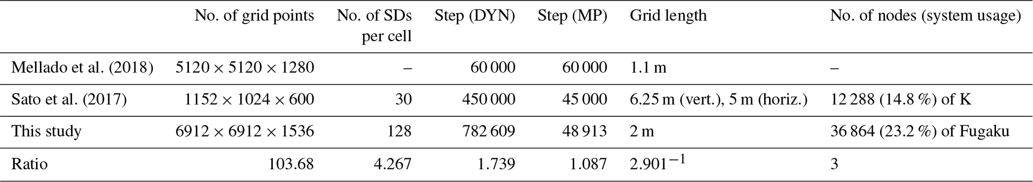
Mellado et al. (2018) used anelastic equations with saturation adjustment for calculating clouds. They performed large-scale numerical experiments using a petascale supercomputer (Blue Gene/Q system supercomputer JUQUEEN at Jülich Supercomputing Centre). We also note that similar numerical experiments with a large number of grid points () were performed by Schulz and Mellado (2019) using the same supercomputer. Meanwhile, Sato et al. (2017) used fully compressible equations with the SDM and performed 6.25 and 5 m resolution simulations of BOMEX using the petascale supercomputer K. The number of time steps for the dynamical process used in Sato et al. (2017) is 1 order of magnitude larger than that used in Mellado et al. (2018). In addition, because of the high computational cost of the SDM, Sato et al. (2017) used fewer grid points though they used 14.8 % of the total system of supercomputer K. We performed meter-scale-resolution numerical simulations of BOMEX with times higher resolution, 104 times more grid points, and 442 times more SDs than Sato et al. (2017), thereby using 23.8 % of the total system of the supercomputer Fugaku. The computational performance of this simulation will be described in detail in Sect. 5.2.
2.3 Target architecture
In this study, we mainly used computers equipped with Fujitsu A64FX processors to evaluate the computational and physical performance of the new model, SCALE-SDM. In this section, we summarize the essential features and functions of the computers.
Table 2Size and bandwidth of the cache and memory for the Fujitsu A64FX processor.

A64FX is a CPU that adopts scalable vector extension (SVE), an extension of the Armv8.2-a instruction set architecture. A64FX has 48 computing cores. Each CPU has four nonuniform memory access nodes called the core memory groups (CMGs). One core has an L1 cache of 64 KiB and can execute SVE-based 512-bit vector operations at 2.0 GHz with two fused multiply–add units. Each CMG shares an L2 cache of 8 MiB and has high bandwidth memory (HBM2) of 32 GB (bandwidth of 256 GB s−1). The theoretical peak performance per node is 3.072 tera floating-point operations per second (TFLOPS) for double precision (FP64). Supercomputer Fugaku has 158 976 nodes with a 6D torus shape. The cache and memory performances, which are particularly important for this study, are summarized in Table 2. A64FX has high memory bandwidth comparable to a GPU. In addition, SVE can execute FP64, single-precision (FP32), 32-byte integer (INT32), 16-byte floating-point number (FP16), and 16-byte integer (INT16) calculations.
Fugaku and FX1000 have a power management function to improve the computational power performance (Grant et al., 2016). Users can control the clock frequency (2.0 GHz or 2.2 GHz) and use one or two of the floating-point pipelines.
The performance of Fugaku is 46 times the peak performance and 30.7 times the memory bandwidth of K. In addition, using FP32 or FP16, the amount of data calculated by single instruction and that transferred from memory doubles or quadruples, respectively, and by optimizing a code according to its characteristics, users can potentially achieve a further 2 or 4 times higher effective peak performance, respectively. Due to the high memory bandwidth of Fugaku, its bytes per flops ratio () is 0.33, which is not too small compared to that of K ().
Although this study describes optimizations for A64FX, most of them can be applied to many-core general-purpose CPUs such as Intel Xeon equipped with x86-64 instruction set architecture. For such generalization, please see Sect. 3.3.1 with the parameters in Table 2 replaced with those for the x86-64 architecture. Optimization using accelerators such as GPUs is beyond the scope of this study. However, since the applicability of this study to accelerators is necessary for future high-performance computing, we discuss some differences between CPU-based and GPU-based approaches.
To map CPU-based optimization to GPU-based optimization, the L1 cache of the CPU can be read as the register file (for storing most frequently accessed data), L1 cache, and shared memory; OpenMP parallelization can be read as streaming multiprocessor parallelization for NVIDIA GPU (or Compute Unite for AMD GPU); and MPI processes can be read as the number of GPUs. In addition, since the memory bandwidth of one node of A64FX is comparable to that of a single GPU (e.g., NVIDIA Tesla V100: 900 GB s−1, A100: 1555 GB s−1), a comparison in terms of memory throughput is reasonable if we assume that all the SD information is on GPU memory. Although the approaches for cache and memory optimization of the CPU and GPU are similar, those for calculation optimization may differ. For example, GPUs are not good for reduction calculations, such as calculating the liquid water content in a cell from the SDs in the cell. The current trend for supercomputers is to use heterogeneous systems comprising both CPUs and GPUs as they provide excellent price performance. Nevertheless, memory bandwidth is essential for weather and climate models, including the SDM. Thus, it is not easy to achieve high performance unless the entire simulation can be handled only in GPUs.
The numerical model UWLCM (Arabas et al., 2015; Dziekan et al., 2019; Dziekan and Zmijewski, 2022) utilized GPUs for the SDM and CPUs for other processes, and Dziekan and Zmijewski (2022) achieved 10–120 times faster computations compared with CPU-only computations. Still, the time to solution using the SDM is 8 times longer than the bulk method. Although the CPU used had a lower bandwidth memory compared with the GPU for the dynamical core and the bulk method, we used a CPU with a higher bandwidth memory for all processes. This is an advantage when the entire simulation must be accelerated to reduce the time to solution.
3.1 Domain decomposition
We used SCALE-RM (Scalable Computing for Advanced Library and Environment-Regional Model; Nishizawa et al., 2015; Sato et al., 2015) as the development platform. We adopted the hybrid type of three- and two-dimensional (3D and 2D) domain decompositions using MPI. For 3D decomposition, we denoted the numbers of MPI processes for the x,y, and z axes as Nx,Ny, and Nz, respectively. For 2D decomposition, we decomposed the x and y axes into and domains, respectively. Here, we set and such that . Then, the total number of MPI processes N is common, i.e., . These two types of domain decompositions were utilized depending on the type of computations. The hybrid type of domain decomposition requires the conversion of grid systems containing every Nz of MPI processes. Note that the cost should not be a significant issue compared to collective communication across the entire MPI processes when Nz is relatively small (Nz<O(100)). The 3D domain decomposition is suitable for dynamical processes because frequent neighborhood communications are required to integrate short time steps for acoustic waves; further, the amount of communication is less because of the small ratio of halos to the inner grids. On the other hand, 2D domain decomposition is suitable for the SDM. As described later, since the number density of SDs is initialized proportional to the air density, the number of computations varies vertically in a stratified atmosphere. In addition, variations in the computation amount and data movement depend on whether clouds and precipitation shafts are within the domain. If 3D decomposition is used, domains without any clouds are likely, e.g., near the top and bottom boundaries; such domains may lead to a drastic load imbalance.
A drawback of the 3D domain decomposition is that it is more likely to suffer from network congestion; further, there will be hardware limitations on the number of simultaneous communications due to the increase in the number of processes in a neighborhood. The number of processes is 26 for 3D domain decomposition, while it is 8 for 2D domain decomposition. In addition, the throughput of communication decreases for smaller message sizes. In this study, we eliminated all unnecessary communications from the diagonal 20 directions and pack communications for each neighborhood direction to the maximum extent possible to gain high communication throughput. Communication time was overlapped with computation time during the dynamics process to reduce the time to solution.
3.2 Initialization of super-droplets
Although the SDM makes fewer assumptions about the DSD, the accuracy of the prediction depends on the initialization of the sampling of SDs from a vast number of real droplets. Shima et al. (2009) first used the constant multiplicity method, which samples SDs from normalized aerosol distribution. Further, Arabas and Shima (2013), Sato et al. (2017), and Shima et al. (2020) used the uniform sampling method, in which SDs were sampled from a uniform distribution of the log of the aerosol dry radius to sample droplets that are rare but important: for example, large droplets that may trigger rain. Indeed, Unterstrasser et al. (2017) showed that collision–coalescence calculations converge faster for a given number of SDs if the dynamic range of multiplicity is broader (i.e., the uniform sampling method), and they converge slower if the constant multiplicity method is used. However, owing to the broad dynamic range of the uniform sampling method, some multiplicities obtained using this method may fall below 1 if too many SDs are used to increase the spatial resolution. In this case, since multiplicity is stored as an integer type, some SDs will be cast to 0, and the number of SDs and real droplets will decrease.
One approach to solve this problem is to allow multiplicity to be a real number (floating-point number) (Unterstrasser et al., 2017). The SDM can handle discrete and continuous systems because its formulation is based on the stochastic and discrete nature of clouds. Nevertheless, simulations using this method may not behave as discrete systems in a small coalescence volume where the Smoluchowski equations do not hold (Dziekan and Pawlowska, 2017).
Another approach to solve the deterioration of multiplicity is to cast multiplicity from a floating-point number to an integer by stochastic rounding (Connolly et al., 2021). For example, let k be an integer, and let us set interval that contains a real number l; then, l rounds to k with probability and to k+1 with probability l−k. Hence, an expected value obtained by the stochastic rounding process is consistent with the original real number l. Thus, the sampling accuracy does not decrease. Although this approach cannot prevent a decrease in the SDs, it can prevent the decrease in the number of real droplets statistically.
However, we can consider these approaches to not be optimal for meter- to submeter-scale-resolution simulations. Unterstrasser et al. (2017)'s discussion was based on the result of a box model, which is a closed system and requires a large ensemble of simulations to obtain robust statistics. In practical 3D simulations, the cloud microphysics field fluctuates spatiotemporally because of cloud dynamics and statistics in finite samples. If we sample a vast number of SDs and if the number of samples becomes close to the actual number of droplets, imposing a constraint on the number is reasonable so that the dynamic range of multiplicity will be small (i.e., more similar to constant multiplicity) and the multiplicity for all SDs will be larger than 1. If such a method is used, we expect rare droplets to exist only in some cells rather than in every cell – this is a more natural continuation toward discrete systems. How can we develop such an initialization method? In addition, previous studies focused on collision–coalescence, but the sensitivity of cloud microphysical variability related to condensation–evaporation to SD initialization must also be considered. Against this background, which type of initialization is better overall?
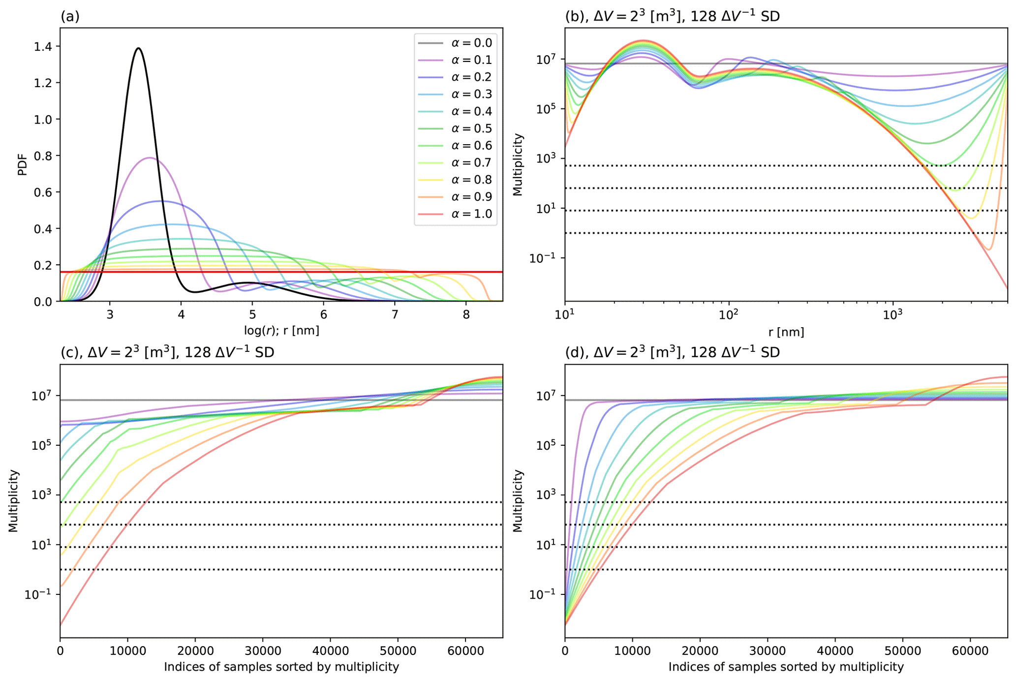
Figure 1(a) Normalized aerosol distribution given by vanZanten et al. (2011) (bold black line) and proposal distributions used for sampling (α=0–1). The bold red line shows the proposal distribution used for the uniform sampling method. (b) Relationship between dry aerosol radius and multiplicity when ΔV=23 m3 and 128 SDs per cell are sampled. (c) Distribution obtained by sampling 216 SDs using the same setup as (b) (ΔV=23 m3 and 128 SDs per cell) and sorted by multiplicity in ascending order. (d) The distribution corresponding to (c) when the L2 norm is used as a metric. The dotted lines in (b), (c), and (d) indicate .
To develop a new initialization method, we considered the simple method of generating a proposal distribution that connects the uniform sampling method to the constant multiplicity method. We chose the log of the aerosol dry radius log r in the interval between rmin and rmax as the random variable. We denote an initial aerosol distribution as n(log r) and its normalization as . The relation between ξ, n, and the proposal distribution p was given by Shima et al. (2020) as
where NSD is the SD number concentration. In the following explanation, we discretize the random variable into k bins and nondimensionalize the bin width to 1 for simplicity.
We define a probability simplex, which is a set of discretized probability distributions as follows:
Let us denote the discretized probability distribution of as b1∈Ck and the uniform distribution as b2∈Ck. Then, we define an α-weighted mean distribution a as the Fréchet mean of b1 and b2:
where ℒ is a metric to measure the distance between two distributions. A distribution a corresponds to a discretized and nondimensionalized proposal distribution of p. When the argument of the optimization is a function, the L2 norm is often used as the metric ℒ. In our case, since the argument is a probability distribution, the Wasserstein distance W2 (Santambrogio, 2015; Peyré and Cuturi, 2019), which is a metric that measures the distance between two probability distributions, is a more natural choice. Several methods have been proposed to obtain solutions in Eq. (5) numerically. One method is to regularize the optimization problem of Eq. (5) by using the entropic regularized Sinkhorn distance Sγ (Cuturi, 2013; Schmitz et al., 2018) (γ is the regularization parameter) instead of the Wasserstein distance . Another method is to use displacement interpolation (McCann, 1997), which is an equivalent formulation of Eq. (5). We used the method based on the Sinkhorn distance with in Sect. 5. In this section and Sect. 4, we used the displacement interpolation specialized for the case in which the random variable is one-dimensional to solve Eq. (5) more accurately. The specific forms of the Wasserstein distance W2, Sinkhorn distance Sγ, and displacement interpolations are described in Appendix A.
We verified this method of generating proposal distributions by adopting a specific aerosol distribution n(log r). We used the bimodal lognormal distribution of vanZanten et al. (2011). This distribution is composed of ammonium bisulfate with a number density of 105 cm−3. We chose the interval for the random variable as rmin=10 nm and rmax=5 µm, and we adopted k=1000 bins and to calculate proposal distributions.
The proposal probability distributions obtained using various α are shown in Fig. 1a. As α decreases, the uniform distribution gradually changes to the normalized aerosol distribution, and probabilities (frequency for sampling) near both ends of the random variable decrease.
The relationships between the aerosol dry radius and multiplicity for cell volume ΔV=23 m3 and 128ΔV−1 SDs are shown in Fig. 1b. Multiplicity for the large dry radius of aerosol falls below 1 for α=1.0 but exceeds 1 for α=0.8 for all samples.
Figure 1c shows the multiplicities of samples that are obtained by sorting 216 SDs by their multiplicity. The influence of α on changing the dynamic range of multiplicity and the number of ξ<1 samples can be clearly observed in Fig. 1c. Since the relationship between the aerosol dry radius and multiplicity does not change relatively with increasing spatial resolution, we indicate ξ=80–83 by dotted lines in Fig. 1c. As α decreases, the dynamic range of multiplicity decreases, and the minimum log multiplicity increases by an almost constant ratio when α≥0.2. When ΔV=1 m3, the multiplicity of all samples exceeds 1 if α≤0.7. Similarly, the multiplicity exceeds 1 when ΔV=503 cm3 if α≤0.6 and when ΔV=253 cm3 if α≤0.5. Since the numbers of samples of ξ<1 and 0.5 account for 7.82 % and 6.70 % of total samples, respectively, many invalid SDs are sampled if the uniform sampling method is used for 2 m resolution.
Figure 1d shows the results corresponding to Fig. 1c obtained for the L2 norm instead of to generate proposal distributions using Eq. (5). In this case, as α decreases, the number of ξ<1 samples decreases (0.413 % of total samples when α=0.1), but the dynamic range of multiplicity does not change unless α=0.0. Thus, these results suggest that the manner of connecting the two distributions is critical.
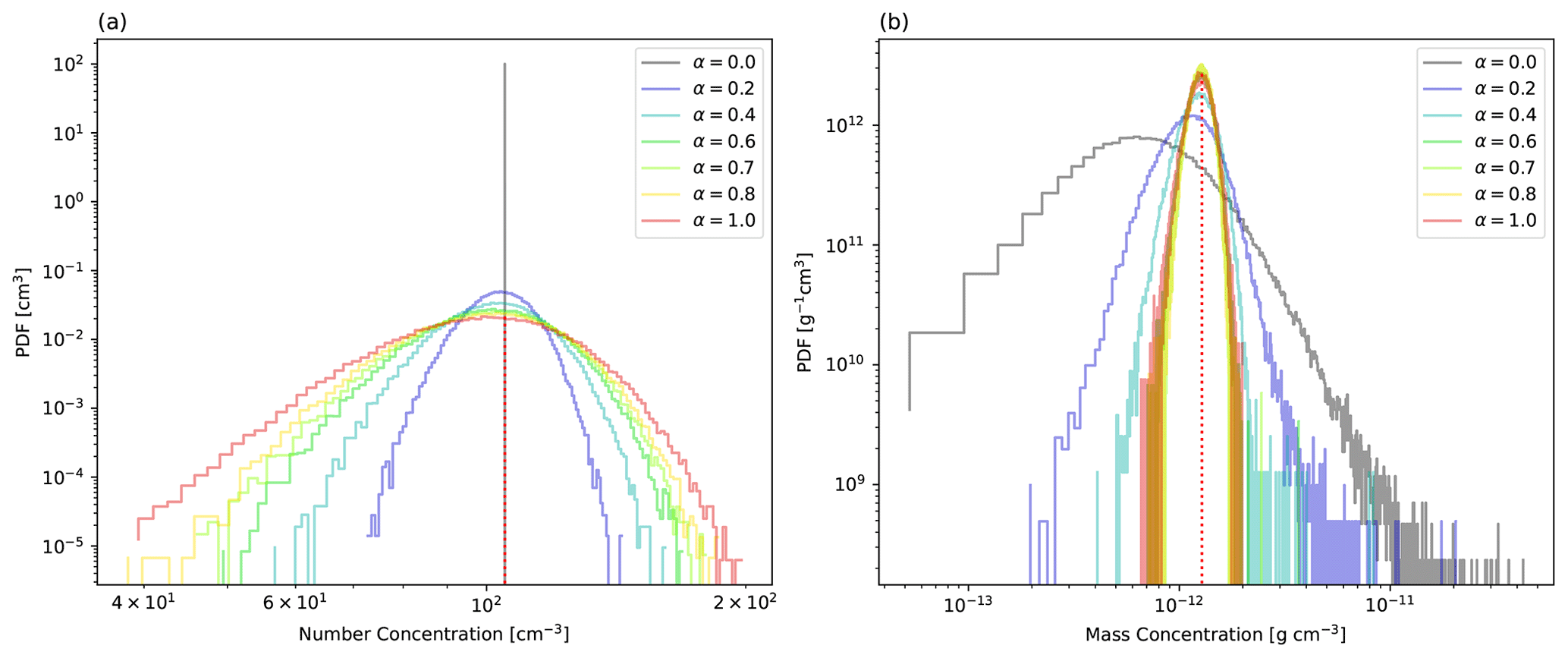
Figure 2Probability distributions of (a) aerosol number concentration and (b) aerosol mass concentration, obtained by sampling from various proposal distributions. The red dotted lines show the exact expected values.
How do aerosol statistics behave if we change α using the above method? The probability distributions of the number and mass concentration of dry aerosol for various α are shown in Fig. 2. We calculated the number and mass concentrations from 128 SDs. The multiplicity was cast to an integer using stochastic rounding for ΔV=23 m3. We performed 105 trials to obtain the probability distributions. The statistics of real droplets, corresponding to the limit when α=0 and the exact expected value, are also shown by a dotted red line in each panel of Fig. 2.
The expected values obtained by applying the importance-sampling method do not depend on the proposal distribution used. However, the variances of the expected values depend on the ratio of the original distribution to the proposal distribution, and they become small when the original and proposal distributions are similar. In fact, the aerosol number concentration distribution is narrow when the proposal distribution used is the same as the original distribution (α=0) (Fig. 2a), and it becomes broader as α increases. Thus, the uniform sampling method introduces significant statistical fluctuations (or confidence interval) of the aerosol number concentration. In contrast, the aerosol mass concentration distribution is narrow when α=1.0, and it broadens as α decreases (Fig. 2b). Thus, the uniform sampling method results in smaller statistical fluctuations of the aerosol mass concentration. That is, as α decreases, the importance sampling for the aerosol size distribution gradually changes its effect from the reduction of the variance of mass concentration to the reduction of the variance of number concentration. We note that the results are almost identical when we store multiplicity as a real-type floating-point number (not shown in the figures).
Based on the above considerations, the proposal distributions for α=0.7 were used for the numerical experiments described in Sect. 5. Although we focused on the statistical fluctuations of the aerosol, α may also be a sensitive parameter influencing the cloud dynamical and statistical fluctuations. Since this aspect is nontrivial because of the effect of cloud dynamics, we will describe the results of the sensitivity experiments for α in Sect. 4.3.
3.3 Model optimization
3.3.1 Strategy for acceleration
Based on the computers described in Sect. 2.3, we devised a strategy for optimizing the SDM. All algorithms used in the SDM have computational complexity of the order of SD numbers. In general, the PIC applications tend to have small due to the large computations involved. This will also hold for the SDM (except for the collision–coalescence process) because of the velocity interpolation to the position of SDs in movement, and the Newton iterations in activation–deactivation involve many calculations. Then, one may expect that a high computational efficiency can be achieved if the information for the grids and information for SDs are both on the cache as this can prevent the memory throughput being a bottleneck for the time to solution. However, since the calculation pattern in the cloud microphysics scheme changes depending on the presence of clouds and particle types, the codes in a loop body are complicated and often include conditional branches. Hence, high efficiency is difficult to achieve because of the difficulty of using SIMD vectorization and software pipelining. In the following paragraphs, we describe optimization based on two strategies: first, we developed cache-efficient codes by cache blocking (e.g., Lam et al., 1991) and reduction of information for the SDs. Second, we simplified the on-cache loop bodies to the maximum extent possible by excluding conditional branches.
We first considered applying cache-blocking techniques to the SDM. Since the L1 cache on A64FX is 64 KiB per core, 32 data arrays, which consist of 83 grids of 4-byte elements (each array consumes 2 KiB), can be stored on the L1 cache simultaneously. Similarly, since the user-available L2 cache is 7 MiB (of 8 MiB)/12=597 KiB per core, two data arrays which consist of 128 SDs per cell ×83 can be stored on the cache if an attribute of SDs consumes 4 bytes. Therefore, we divide the grids into groups of less than 83 (hereafter called “blocks”) for cache blocking. For each cloud microphysics process, we integrated all SDs by one time step forward and then moved on to the next process. In the original SDM, a single loop is used for all SDs in the MPI domain. In this study, we decomposed this single loop for all SDs into loops for all blocks and all SDs in each block; subsequently, we parallelized the loop for all blocks using OpenMP through static scheduling with a chunk size of 1. Although applying dynamic scheduling to the loop for all blocks may improve load balancing among blocks, it is difficult to validate the reproducibility of the stochastic processes, such as collision–coalescence, because random seeds may change with every execution.
To simplify the loop body for the SDs in a block, it is essential that the gridded values in a block are a collection of similar values because similar operations or calculations may be applied to these values in such cases. The effective resolution of atmospheric simulations (Skamarock, 2004) imparts such numerical effects on the grid fields. The volume, which consists of 83 grids, is comparable with the volume of effective resolution, which is the smallest spatial scale at which the energy spectrum is not distorted numerically by the spatial discretization. For example, since the energy spectrum obeys the law roughly in the inertial range for LES, we regard the effective resolution as the smallest spatial scale at which the energy spectrum follows the law. The typical effective resolution is 6Δ–10Δ for planetary boundary layer turbulence, which may depend on the numerical accuracy of the spatial discretization of basic equations as well as the filtering length and shape of LES. The physical interpretation of effective resolution is that the flow is well resolved if the spatial scale is larger than 6Δ–10Δ, and the variability decreases exponentially for scales smaller than this range. We used this prior knowledge to simplify the loop body, as described later.
3.3.2 Super-droplet movement
To save computational cost of the SDM, it would be advantageous to maintain the SD number density in areas where clouds are more likely to occur. This can be achieved by resampling the SDs in clouds using methods such as SD splitting and merging proposed by Unterstrasser and Sölch (2014), thereby optimizing the collision–coalescence calculations. Alternatively, one can automatically adjust the SD number density following the SD movement. We describe the second approach in detail.
To maintain the SD number density in clouds globally, we can initially place an increased number of SDs in the computational domain so that the SD number density is proportional to air density. For example, when the parcel is lifted, the SD number density decreases but may be maintained at the same level as the surrounding SD number density. However, this requires designing the SD movement scheme so that the time evolution of the SD number density follows the changes in air density. We focus on such schemes for grid-scale motion since the effect of subgrid motion should be relatively small. Because the air density decreases by the divergence of the velocity fields, the interpolation of the velocity should be developed to provide the divergence at the position of SDs that are calculated from interpolated velocity equal to divergence at the cell. For such a scheme, a reduction in the variability of the SD number density is also expected since the divergence at the SDs does not differ within a cell.
In addition to ensuring consistency between changes in SD number density and air density in velocity interpolation, numerical accuracy of the interpolation may also be necessary if small eddies and mixing are resolved in LES. Because the SDM is free from numerical diffusion by solving the SD movement in a Lagrangian manner, an interpolation scheme of higher order than the first-order scheme (Grabowski et al., 2018) may not significantly directly affect the phenomena whose spatial scale is sufficiently larger than the grid scale. However, as the flow within a cell is always irrotational and is first-order convergent with respect to grid length, the first-order scheme can deteriorate the numerical accuracy of meter- to submeter-scale eddies. Furthermore, it can affect large-scale phenomena through interactions between eddies and microphysics.
In this study, a second-order spatial-accuracy-conservative velocity interpolation (CVI) is developed on a 3D Arakawa C-grid with these properties. While the CVIs of the second-order spatial accuracy on 2D grids have been used in various studies such as Jenny et al. (2001), few studies have explored such CVIs on 3D grids. Recently, a CVI for a divergence-free velocity field on a 3D A-grid was developed by Wang et al. (2015). We extend the method used in their study for the nondivergence-free velocity field on the C-grid. The accuracy of the interpolation is of second order only within the cell, and we allowed discontinuous velocity across the cell. The derivation of our CVI using symbolic manipulation (Python SymPy) is available in Matsushima et al. (2023b). We only provide the specific form of the CVI in Appendix B.
The number of grid fields necessary to compute Eqs. (B7)–(B12) is important for computational optimization. While 24 elements (3 components × 8 vertices in a cell) are necessary to calculate the velocity at an SD position for trilinear interpolation (and the same applies for second-order CVI on the A-grid), only 18 elements are necessary for the second-order CVI on the C-grid (Eqs. B7)–(B12). That is, we can reduce 25 % of the velocity field data that occupy the L1 cache and use the remaining cache for SDs. The change in the spatial distribution of SDs through SD movement considering the spatial accuracy of CVI will be discussed in Sect. 4.2.
For warm clouds, since the information for the SD position accounts for half of all attributes, reduction of these data without loss of representation and prediction accuracy contributes greatly to saving the overall memory capacity in the SDM. However, using FP32 instead of FP64 may cause critical problems due to the relative inaccuracy and nonuniform representation in the domain in the former case. In the following paragraphs, we describe these problems and a solution.
In the original SDM, the SD position is represented by its absolute coordinate over the entire domain, but this method requires many bits. However, since we already decomposed the domain into blocks, using the relative position of SDs in a block is numerically more efficient. For this case, we can reduce the information per SD by subtracting the information that arises from the partitioning of the domain by the MPI process and a block from the global position.
If we represent the position of SDs as a relative position in a block, additional calculations are necessary when an SD crosses a block. Such calculations introduce rounding errors for the SD position, and the cell position where the SD resides may not be conserved before and after its calculations. Let us consider an example. Consider a block that consists of a grid. Let us define the relative position x of SDs belonging to and the machine epsilon for the precision of floating-point numbers as ϵ. If SD crosses to the left boundary and reaches , the relative position of the SD is calculated by adding the values of right boundary 1 in a new block to the SD position: . However, rounding to the nearest new position results in the following: . For FP32, since µm if we adopt meters as units, we expect this does not happen frequently. However, if such a case occurs even with only one SD of the vast number of SDs in the domain, the computations may be terminated by an out-of-array index. Although a simple solution is exception handling using min–max or floor–ceiling, this solution may deteriorate the computational performance by making the loop bodies more complex, and the correction bias introduced by exception handling may be non-negligible when low-precision arithmetic is used. To ensure safe computing, the suitable approach is to calculate the relative position without introducing numerical errors.
In this study, we represent the relative position using fixed-point numbers. This format allows us to define the representable position of SDs so that they are uniformly distributed in the domain, and integer-arithmetic-only calculations are used. Then, the same problem as in the case of simply using floating-point numbers does not arise in principle. Let us denote the range for which the SD is in cell k as and number of grid points along an axis as b. Then the range of positions in a block is represented as . We define the conversion from z∈Z to its fixed-point number representation q as the following affine mapping:
When b≤8, s=21 and when FP32 is used instead of INT32, the range of is accurately represented by the mantissa of the floating-point numbers, and the representation does not exceed the representable range if it is only a few grids outside a block. With regard to the velocity, the amount of movement per step is represented using a fixed-point number. We used FP32 instead of INT32 for the actual representation because the representable range of fixed-point numbers is small and could easily exceed its range by multiplication.
By using relative coordinates for the SD positions within a block, the precision of their locations is varied when Δz is changed. This is because the change of position in real space is 2−sΔz from Eq. (6) when the grid length is Δz, and the variation in q is 1; this value is reduced for smaller Δz. In addition, the change in the relative position per time step is 2sviΔtΔz−1 when the time step is Δt; hence, it increases as Δz decreases, thus providing a better representation of the relative position. Δt is set sufficiently small to ensure there is no large deviation from the time step of tracer advection. Then, the change in the relative position does not change if the ratio of Δt to Δz is kept constant. In real space, the numerical representation accuracy of position and the arithmetic operation accuracy of the numerical integration vary with the spatial resolution and time step. Therefore, we can maintain numerical precision for meter-scale-resolution simulations.
In terms of I/O, fixed-point numbers facilitate easy compression. For example, the interval of representable positions q in real space with Δz=2 m and a block size of 8 is 0.95 µm; this yields higher accuracy than the Kolmogorov length of 1 mm and is thus always excessive as a representation for DNS and LES. We can discard unnecessary bits when saving data on a disk.
3.3.3 Activation–condensation
The timescale of activation–deactivation of the cloud condensation nuclei (CCN) is short if the aerosol mass dissolved in a droplet is small (Hoffmann, 2016; Arabas and Shima, 2017). Hence, the numerical integration of activation–deactivation is classified as a stiff problem. To solve Eq. (2), Hoffmann (2016) used the fourth-order Rosenbrock method with adaptive time stepping. SCALE-SDM employs the one-step backward differentiation formula (BDF1) with Newton iterations. Although BDF1 has first-order accuracy, it has good stability because it is an L-stable and implicit method, and we can change time intervals easily because it is a single-step method. However, with the implicit method, Newton iterations must be performed per SD, and the number of iterations required for convergence of the solution differs for each SD, thereby making vectorization a complicated task. To overcome this difficulty, the original SDM uses excessive Newton iterations (20–25) that are sufficient for all SDs to converge, assuming that numerical experiments are performed on a vector computer such as the Earth Simulator. However, we cannot tune codes for both vector computers and short-length vector computation by using SIMD instructions in the same way. In the original SDM code, the loop body of time evolution by Eq. (2) is very complex because of the presence of conditional branches, grid fields at the SD position, and iterations; hence, it cannot issue SIMD instructions. Therefore, we devised a method to allow SIMD vectorization based on the previously described strategy.
Equation (2) is discretized by BDF1 as
where p is the current droplet radius, and R is the updated droplet radius. Equation (7) has at most three solutions; in other words, one or two of them may be spurious solutions. However, the uniqueness of the solution is guaranteed analytically in the following two cases (see Appendix C for derivation). Case 1, which depends on Δt, is
and Case 2, which depends on the environment and initial condition, is
Case 1 implies that an activation timescale restricts the stable time step for each SD. Based on the estimation of temperature T=294.5 K at z∼600 m in the BOMEX profile, when α=0.7, 87.7 % of SDs satisfy the condition for Case 1 if Δt=0.0736 s, 91.0 % if , and 100 % if . Similarly, when α=0.0, 91.4 % of SDs satisfy the condition if Δt=0.0736, 97.6 % if , and 100 % if . The smaller the value of α, the smaller the frequency of sampling small droplets and the greater the number of SDs that satisfy the condition.
On the other hand, Case 2 is a condition for the initial size of droplets p in an unsaturated environment. In the BOMEX setup, since cloud fraction converges at a grid length of 12.5 m (Sato et al., 2018), we can estimate the ratio of SDs that satisfy Case 2 for higher resolutions by analyzing the results of similar numerical experiments using new SCALE-SDM. We define droplets of the size as aerosol particles (or haze droplets) and droplets that are larger than and smaller than 40 µm as cloud droplets. We do not provide the detailed results, but the ratio of air density weighted volume (i.e., mass) where cloud water exists in a cell to the total volume in the BOMEX case is approximately 1.5 % in a quasi-steady state based on the numerical experiments with our developed model. Therefore, we estimate that 98.5 % of SDs satisfy the condition of Case 2 in the BOMEX setup.
Hence, if we ensure the uniqueness of the solution by Case 1 for a cloudy cell and Case 2 for a cell with no clouds, the frequency of exception handling during Newton iterations can be largely reduced. We first check whether we need a conditional branch of the unsaturated environment (of Case 2). Since the block has a small volume that is comparable with the effective resolution, as discussed in Sect. 3.3.1, we can convert the conditional branches of the unsaturated condition for an SD to that for all SDs in a block with little or no decreasing ratio of SDs to satisfy the condition. This conversion of the conditional branch allows a loop body of time evolution by Eq. (7) to be simple and specific to Case 2. There is an exception: when the initial size of droplets is larger, it is handled individually only if such droplets exist in a block. If the environment is saturated, we ensure the uniqueness of the solution with Case 1. In this case, we list the SDs that satisfy Case 1 and perform Newton iterations according to the list. Other SDs are calculated individually and using adaptive time stepping for unstable cases.
By using this method, we find that almost all SDs satisfy the uniqueness condition of the solution, and we should only focus on optimizing these SDs. For tuning, the SDs in a block are classified into groups of 1024 SDs (which fit in the L1 cache), and each division calls the process of activation–condensation. In each call, the time evolution of each SD is calculated. A single loop for the updates of droplet radius calculates two iterations because this is the maximum number of Newton iterations that can allow SIMD vectorization and software pipelining without register spill of 32 registers with the current compiler we used for A64FX. The loop is repeated for all SDs in a division and breaks if the squares of all droplet radii of SDs fall below the tolerance relative error of 10−2. Since the loop is vectorized by SIMD instructions and the number of iterations is often limited to two if we use the previous droplet radius for the initial value for the Newton iterations, the computational time for activation and condensation is drastically less than that of the original SDM, as shown later.
Note that the most frequently encountered case might depend on the type of simulated clouds. For example, Case 2 is more often selected in an experiment when clouds occupy a large fraction of the total domain volumes. However, the calculations of both cases are almost identical; hence, the computational performance depends more on the number of iterations (i.e., the closeness between the initial guess and solution) than the differences between the cases.
3.3.4 Collision–coalescence
The computational cost of the collision–coalescence process is already low for the algorithm developed by Shima et al. (2009). We reduced the computational cost and data movement further rather than achieving a higher efficiency against theoretical peak performance of floating-point number operations. Since we used only the Hall kernel for coalescence, the coalescence probability was small for two droplets of small and similar sizes. Therefore, it is reasonable to ignore the collision–coalescence process in cells with no clouds. Notably, no cloud condition can precisely match Case 2 described in Eq. (9). If even a single cloud droplet exists in a block, it becomes necessary to sort the cell indices of all SDs in the block. However, we can remove sorting if cloud droplets do not exist in a block. We do not sort the attributes of the SDs with cell indices as a key since they are already sorted with a block as a key, as will be described in Sect. 3.3.5. Further, some attributes are on the L2 cache during the collision–coalescence process due to cache blocking. By not sorting the attributes of the SDs, the write memory access of SDs that do not coalesce is avoided. In the BOMEX setup, 98.5 % of the SDs satisfy Case 2 and we do not calculate the collision–coalescence of these SDs. Therefore, we expect a drastic reduction in the computational cost and data movement in some cases in which cloudy cells occupy only a small fraction of the total domain volume. This method to reduce the computational cost potentially leads to a large imbalance as in the Twomey SDM by Grabowski et al. (2018). However, we also expect that the imbalance might be mitigated better as cache blocking improves the worst-case elapsed time among the MPI processes.
3.3.5 Sorting for super-droplets
To utilize cache blocking effectively during the simulation, the SDs in a block should be contiguous on memory. This is possible if we sort the attributes of the SDs using the block ID as the sorting key when SDs move out of one block to another. This sorting is different from the usual sorting in which each block can send SDs to any other block; in the present sorting, the direction of SD movement is limited to adjacent blocks along x, y, and z axes. Such sorting is commonly used in the field of high-performance computing. Although we did not make any novel improvement, we summarize this process because it is essential to our study, and some readers may not be familiar with on-cache parallel sorting for the PIC method used during computation (Decyk and Singh, 2014).
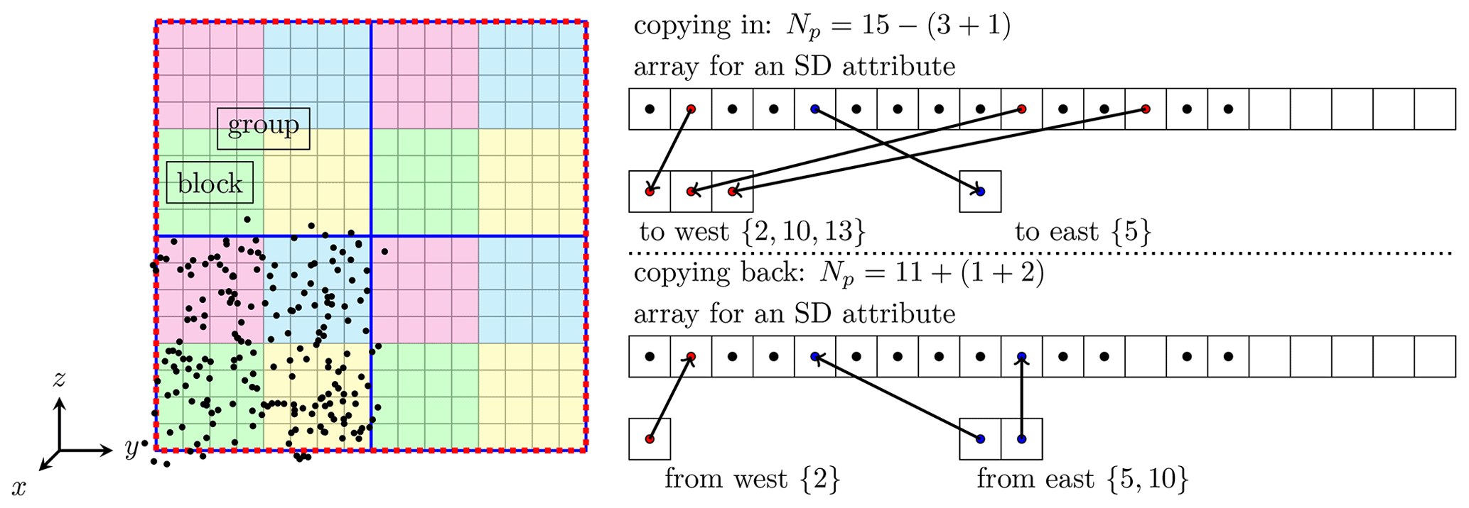
Figure 3Data hierarchy (particle and cell, block, group) in each MPI process and algorithm for SD sorting toward the x direction in each block. In the example, an MPI process has four groups, a group has four blocks, and a block has 4×4 cells. Using a list ({}) that stores the indices, SD sorting is completed by copying in the SDs moving to adjacent blocks and copying back the SDs moving into the block. The number of total SDs within a block is monitored by counting only the moving SDs.
Since memory bandwidth generally limits sorting performance, it is essential to reduce data movement. In our case, the directions of data movement are limited, and most of the SDs in a block are already sorted. We should adopt a design such that these data are not moved and any unnecessary processes are not performed. We should also reduce the buffer size for sorting because of the low memory capacity of A64FX, perform parallelization, and reduce computational costs. However, ready-made sorting, such as the counting sort, may not meet these requirements. Moreover, in the worst case, such sorting may be slower than the main computation in the SDM because of random access in the memory.
In this study, we sorted the attributes of SDs in three steps along the x, y, and z axes. Data hierarchy within each MPI process and an example of one-dimensional SD sorting are shown in Fig. 3. Each step requires at least two loops: copying in the SDs moving to adjacent blocks and copying back the SDs moving into the block. Since the SDs in a block either stay in the same block or only move one block forward or backward, we did not sort the attributes of SDs with combinations as a key. Instead, we made a list of SDs to move to reduce the computational costs and unnecessary data movement. Copying in and back of the SDs to the working array should be divided into small groups so that size of the working array for SDs is reduced by divisions. A loop for a block in each step can be parallelized naturally by using OpenMP. Although a few invalid SDs (buffer) may be included in the arrays, this study does not attempt to defragment them explicitly, expecting that the SD movement and sorting with blocks as a key per microphysical time step may cause defragmenting.
This sorting can avoid the problems of using a ready-made algorithm. The drawback of the current implementation is that a larger buffer space is necessary for SD attribute arrays because a block has few grids and the statistical fluctuation of the number of SDs within a block is large. However, this can be improved if we adaptively adjust the size of SD attribute arrays in a block according to air density and statistical fluctuations of SD numbers.
4.1 Methodology of performance evaluation
We evaluated the computational and physical performances of the numerical models and microphysics schemes by comparing the results of the new SCALE-SDM with those obtained with the same model but using the conventional cloud microphysics schemes as well as with the results obtained with the original SCALE-SDM. When comparing cloud microphysics schemes based on different concepts, we should first consider convergence in spatiotemporal resolutions. The two-moment bulk method imposes empirical assumptions on the DSD, leading to less spatial variability or no dependency on the spatial resolution, such as the spectral width of the DSD. However, this does not mean that the simulated microphysics variables can converge quickly to increase the spatial resolution; rather, this indicates that fair comparison in terms of spatial resolution is difficult in principle. Because the bulk method solves the moments of the DSD, one may assume that the timescale of the moments of the DSD might be larger than that of droplets. However, Santos et al. (2020) performed eigenvalue analysis for a two-moment bulk scheme and found that a fast mode (<1 s) also exists in the bulk scheme, which does not considerably deviate from the timescale of individual droplets. Based on this fact, we use the same spatiotemporal resolutions to compare the two-moment bulk method and sophisticated microphysics schemes.
Our optimization goal was to enable meter- to submeter-scale-resolution experiments of shallow clouds to reduce uncertainty and to contribute to solving future societal and scientific problems. Therefore, we adopted a goal-oriented evaluation method instead of estimating the contributions of various innovations for improving the time to solution. Here, we describe the evaluation of the time to solution and data processing speed (throughput) to ensure the usefulness of our work for solving real problems. The throughput for the microphysics scheme, including the tracer advection of the water and ice substances, is defined as follows:
where the number of steps and elapsed time correspond to the microphysics scheme. To compare the cloud microphysics scheme that is based on different concepts, we defined the throughput for a bulk and a bin method by total tracers, including all categories (e.g., water and ice) and statistics (e.g., number and mass). In contrast, we defined the throughput for the SDM by sampling sizes in the data space . This is because we can add any attributes with less computational cost and fewer data movements, and the effective number of attributes may change during time integration; hence, considering many attributes for defining throughput is inappropriate. For example, because we give an initial value of R as a stationary solution of the Eq. (2), R, ξ, and M are initially correlated. We note that the number of tracers does not account for the water vapor mass mixing ratio. An increasing number of tracers or SDs improves the representation power for microphysics. Such an increase in the representation power can be easily achieved for a bin method and the SDM, but is difficult for a bulk method. We do not incorporate the number of SDs that are actually needed to obtain converged solutions into the metric in Eq. (10) to avoid loss of generality, and we will separately discuss the SD numbers. For example, the convergence properties can depend on the variable to be checked, including liquid water content, cloud droplet number concentration, and precipitation. They can also depend on the setup and results of simulations, such as cloud form, number of CCN, probability distributions used for initialization, and random number properties.
To evaluate physical performance, we should confirm that we obtained qualitatively comparable results faster with the SDM than with the original SDM. In terms of throughput, we should also confirm that we obtained qualitatively improved numerical solutions if the elapsed time was approximately the same.
Next, we briefly describe the original SCALE-SDM and other cloud microphysics scheme used for performance evaluation. We refer to the SCALE-SDM version 5.2.6 (retrieved 6 June 2022 from Bitbucket, contrib/SDM_develop) as the original SCALE-SDM. Meanwhile, we used the develop branch, which branches off from version 5.4.5. The new SCALE-SDM also includes a modification from SCALE version 5.4.5 to generate an initial condition of water vapor mass mixing ratio that is similar to that generated by the original SCALE-SDM. The original SCALE-SDM was used only for numerical experiments with the “original” SDM, as labeled hereinafter. When focusing on some differences among cloud microphysics schemes, we will refer to the SDM schemes associated with new SCALE-SDM and original SCALE-SDM as SDM-new and SDM-orig, respectively.
For the microphysics scheme, we used the Seiki and Nakajima (2014) scheme as a two-moment bulk method and the Suzuki et al. (2010) scheme as a (one-moment) bin method, both implemented in SCALE. The Seiki and Nakajima (2014) scheme solves the number and mass mixing ratio of two water and three ice substance categories, while the Suzuki et al. (2010) scheme solves the mass mixing ratio of each bin in discretized DSD for water and ice substances. We considered liquid-phase processes in the bin method and considered liquid- or mixed-phase processes (only for discussion in Sect. 6.1) in the bulk scheme. We also introduced the subgrid-scale evaporation model (Morrison and Grabowski, 2008) in the Seiki and Nakajima (2014) scheme for comparison with the SDM later, which considers a decrease in the cloud droplet number, depending on the entrainment and mixing scenario controlled by a parameter m (ranges from 0, indicating homogeneous mixing, to 1 for inhomogeneous mixing). We did not consider the delayed evaporation by mixing (Jarecka et al., 2013) because of the increased computational cost, which should be addressed in the future work. General optimization has been applied to the Seiki and Nakajima (2014) scheme. In this scheme, SIMD instructions vectorized the innermost loop for the vertical grid index, performing complex calculations on each water substance. The innermost calculations are divided by separate loops to improve computational performance using cache. However, there may still be room to find optimal loop fission and reordering calculations to reduce the latency of operations. In terms of computational cost, optimization is applied to the Suzuki et al. (2010) scheme. However, the innermost loops for bins are not vectorized for a small number of iterations. The future issues for optimization of the mixed-phase SDM are discussed in Sect. 6.1. SCALE adopts terrain-following coordinates and contains features of map projection as a regional numerical model. However, since any additional computational cost and data movement for these mappings cannot be ignored for meter-scale-resolution simulations, we excluded these features in the new SCALE-SDM for the dynamical core, turbulence scheme, and microphysics scheme.
4.2 Warm-bubble experiment
We first evaluated the computational and physical performances via simple, idealized warm-bubble experiments. The computational domain was km for x, y, and z directions. For the lateral boundaries, doubly periodic conditions were imposed on the atmospheric variables and positions of the SDs. The grid length was 100 m. The initial potential temperature θ, relative humidity (RH), and surface pressure Psfc were as follows:
The air density was given to be in hydrostatic balance. We provided a cosine-bell-type perturbation of the potential temperature θ′ to the initial field to induce a thermal convection:
For the SDM, the initial aerosol distribution was the same as that in vanZanten et al. (2011). For the two-moment bulk and bin methods, we used Twomey's activation formula and activated CCN (CCNact) to cloud droplets according to the supersaturation (S) as CCNact=100S0.462 cm−3. We used the mixing scenario parameter m=0.5 in the two-moment bulk method as a typical value for the pristine case in Jarecka et al. (2013). The uniform sampling method was used to initialize the aerosol mass dissolved in a droplet and multiplicity. In the SDM-orig, SDs were initialized so that they were randomly distributed in the domain. In contrast, for SDM-new, SDs were initialized such that the SD number density was proportional to air density. In addition, to reduce the statistical fluctuations caused by a varying number of SDs in space, we used the Sobol sequence (a low-discrepancy sequence) instead of pseudorandom numbers in the four-dimensional space of positions and aerosol dry radius in each block.
For the computational setup, the domain was decomposed to four MPI processes of one node in the y direction using FX1000 (A64FX, 2.2 GHz). Local domains in each MPI process were further decomposed into blocks of size for x, y, and z directions to apply cache blocking for SDM-new. For the numerical precision of floating-point numbers, FP64 was used for the dynamics, two-moment bulk method, bin method, and SDM-orig. In contrast, SDM-new uses mixed precision, but calculations for SDs were primarily performed by FP32. For time measurement, we inserted MPI_Wtime and barrier synchronization at the start and end of the measurement interval. In this experimental setting, there were no background shear flows, and the simulated convective precipitation systems were localized and stationary in some MPI processes, thereby imposing a huge load imbalance of computational costs. However, the execution time was almost the same in the presence and absence of barrier synchronization owing to the stationarity of convective precipitation systems. In addition, if the measurement interval was nested, the times measured in its lowest level of nests did not include the wait time between MPI processes. To this end, we evaluated the performance of each microphysics subprocess without additional time. Time integrations were performed for 1800 s by using Δtdyn=0.2 s for dynamics and Δt=1.0 s for other physics processes.
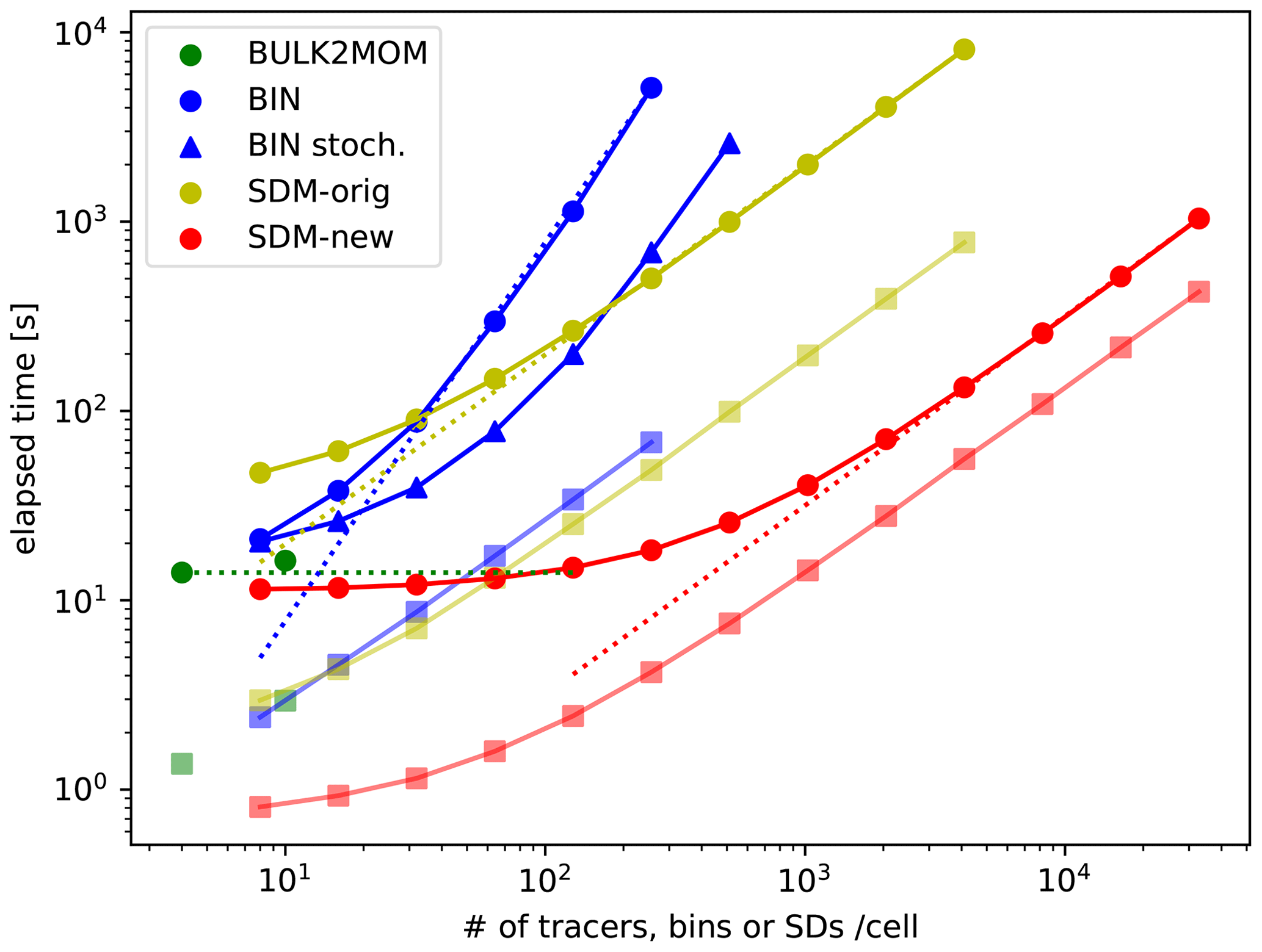
Figure 4Elapsed times of the total (circles) as well as tracer advection and SD tracking (squares) using the two-moment bulk method (green), bin method (blue), SDM-orig (yellow), and SDM-new (red) with different numbers of tracers or mean SDs per cell. Elapsed times of the total (triangles) using the bin method with stochastic collision–coalescence algorithms are also shown. Here, SD tracking included SD movement and sorting with a block as a key. The dotted blue line is the line proportional to N2. The dotted red and yellow lines are lines proportional to N. The dotted green line indicates a constant determined by N. Here, N is the number of tracers, bins, or SDs per cell.
Figure 4 shows the elapsed times of the warm-bubble experiments for various cloud microphysics and different numbers of tracers or SDs per cell. Here, we show only the elapsed times of those numerical simulations that were completed in less than 3 h and that required less than 28 GB of memory. The elapsed time obtained using the bin method (BIN) behaves as O(N2) because all possible pairs of droplet size bins N are considered for calculating collision–coalescence, while that of the SDM-orig behaves as O(N), indicating that the collision–coalescence calculation developed by Shima et al. (2009) reduces the elapsed time. Sato et al. (2009) proposed that the possible combinations of collision–coalescence of the bin method () could be reduced using Monte Carlo integration, which is similar to the SDM; hence, Fig. 4 also shows the results using this option, in which we use , and 4096 for , and 512, respectively. We should use M∝N for reducing the order of the computational complexity to O(N). However, when we set the number of bins to N≥128, the computations were terminated due to large negative values of liquid water that fixers cannot compensate for. This is consistent with a previous study (Sato et al., 2009), which stated that should be used. If we can use this option stably in the future, the elapsed time of the bin method would become comparable to that of SDM-orig. Even if we consider the above point, the SDM-new drastically reduced the elapsed time compared to the bin method for the same number of bins or SDs. Moreover, the elapsed time obtained using the SDM-new with 128 SDs per cell was about the same as that obtained using the two-moment bulk method (BULK2MOM).
The results seem to contradict the intuition that computations using sophisticated cloud microphysics schemes take more time than simpler schemes because of the high computational costs of the former. The main reason for the present results is related to the tracer advection and SD tracking, which is a bottleneck for the elapsed times, as described below, rather than to other cloud microphysics subprocesses. The elapsed times of tracer advection and SD tracking are shown in Fig. 4. The elapsed times of tracer advection and SD tracking obtained using the bin method and SDM-orig are comparable and increase as O(N). For small N, the elapsed time of tracer advection and SD tracking for the SDM-new up to 32 SDs per cell is shorter than that for the two-moment bulk method, which is advantageous in terms of the elapsed time of simulations.
The advantages of SDM-new against the two-moment bulk for calculating tracer and SD dynamics are fewer calculations, higher compactness, and more reasonable use of low-precision arithmetic for SD tracking than for tracer advection. While tracer advection requires a high-order difference scheme to reduce the effect of numerical viscosity, SD tracking does not require a high-order scheme. We used Fujitsu's performance analysis tool (fapp) to measure the number of floating-point operations (FLOPs). We found 303.915 FLOPs per grid and tracer for tracer advection (UD5) excluding FCT and 164.3 FLOPs per SD for SD movement using CVI of second-order spatial accuracy. Since the calculation of UD5 requires values at five grids and halo regions of width 3 in each direction, the calculations are not localized, and a relatively larger amount of communication is necessary. For SD tracking, the calculations for a single SD require only grids that contain the SD, and communication is necessary only when the SD moves out of the MPI process. If FP32 is used for tracer advection, one of the advantages of the SDM-new over the two-moment bulk method is lost. However, the calculations of tracer advection require differential operations, which may cause cancellation of the significant digits. This likely cannot be ignored for high-resolution simulations where the amplitude of small-scale perturbations from the mean state decreases, especially for variables that have stratified structures (e.g., water vapor mass mixing ratio). On the other hand, for the proposed SD tracking, numerical representation precision of the SD positions in physical space becomes more accurate as the grid length and time interval decrease simultaneously. Therefore, the use of FP32 for high-resolution simulations is reasonable. Of course, another important factor behind these results is the fact that the calculations of other SDM subprocesses are no longer bottlenecks in SDM-new.
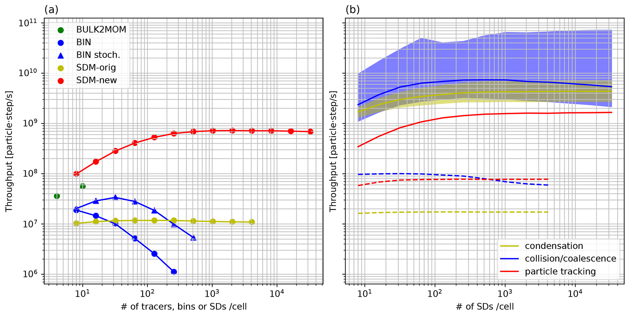
Figure 5(a) Data throughput of microphysics for using the two-moment bulk method (green), bin method (blue), bin method with stochastic collision–coalescence algorithms (blue triangles), SDM-orig (yellow), and SDM-new (red) with different numbers of tracers or mean SDs per cell. (b) The mean data throughput of SD tracking (SD movement and sorting with a block as a key), condensation process, and collision–coalescence using SDM-orig and SDM-new with different numbers of mean SDs per cell. The dotted lines and solid lines show the mean data throughput for SDM-orig and SDM-new, respectively. The range between the minimum and maximum throughputs of condensation and collision–coalescence for SDM-new is indicated by the colors because the load imbalance is significant for only SDM-new.
Now, we compare computational performance among different cloud microphysics schemes in terms of data throughput. The throughput of the microphysics scheme (tracer advection, SD tracking, and microphysics subprocesses) for a different number of mean SDs per cell is shown in Fig. 5a. The throughput of the bin method decreases as the number of bins increases, while that of the SDM-orig remains almost constant but shows a slightly decreasing trend as the number of mean SDs per cell increases. The throughput of both methods is smaller than that of the two-moment bulk method; hence, the elapsed time does not become smaller than that obtained using the two-moment bulk method. In contrast to SDM-orig, the throughput of SDM-new is similar to that of the two-moment bulk method for eight SDs per cell, and it increases as the number of SDs increases. Because of the increase in the throughput, which is related to the increased computational performance and the grid calculations, the elapsed time obtained using the SDM-new increases more gradually than linearly with the increasing number of SDs. Hence, the elapsed time becomes comparable with that obtained using the two-moment bulk method even for larger SDs (∼256). However, as with the SDM-orig, the throughput of the SDM-new shows a decreasing trend when the number of mean SDs per cell exceeds 1024. The maximum throughput of the SDM-new is 61.3 and 20.1 times that of SDM-orig and two-moment bulk method, respectively.
The throughputs of subprocesses obtained by SDM-orig and SDM-new are shown in Fig. 5b. The throughputs obtained by SDM-orig are almost constant with respect to the number of SDs per cell. As the number of SDs increases, the throughput of SD tracking converges to a constant, and the throughput of collision–coalescence decreases from approximately 256 SDs per cell. The throughput obtained by SDM-new is larger than that obtained by SDM-orig for all subprocesses. As the number of mean SDs per cell increases, the throughputs of SD tracking and condensation increase and converge to constants. The throughput of collision–coalescence increases to about 256 SDs per cell but then decreases as in the case of SDM-orig. The minimum throughput of collision–coalescence behaves as the mean throughput, while the maximum throughput increases as the number of SDs per cell increases. This finding reflects the fact that the throughput decreases only in MPI processes that contain clouds in the domain because the L1 and L2 cache miss ratio increases because the random access in the cache and memory during collision–coalescence calculations increases for a large number of SDs. The maximum throughputs of SD tracking, condensation, and collision–coalescence obtained by the SDM-new are 21.3, 251, and 73.1 times that obtained by SDM-orig, respectively. In this study, we did not examine the contributed innovations for the acceleration of the throughput in detail. However, the acceleration rate of the throughput is roughly explained by SIMD vectorization (×16) for SD tracking and also reduced computational cost by terminating Newton iterations faster () for condensation. Before optimization, the condensation calculations were the bottleneck of SDM-orig. After optimization, SD tracking calculations were the bottleneck of SDM-new.
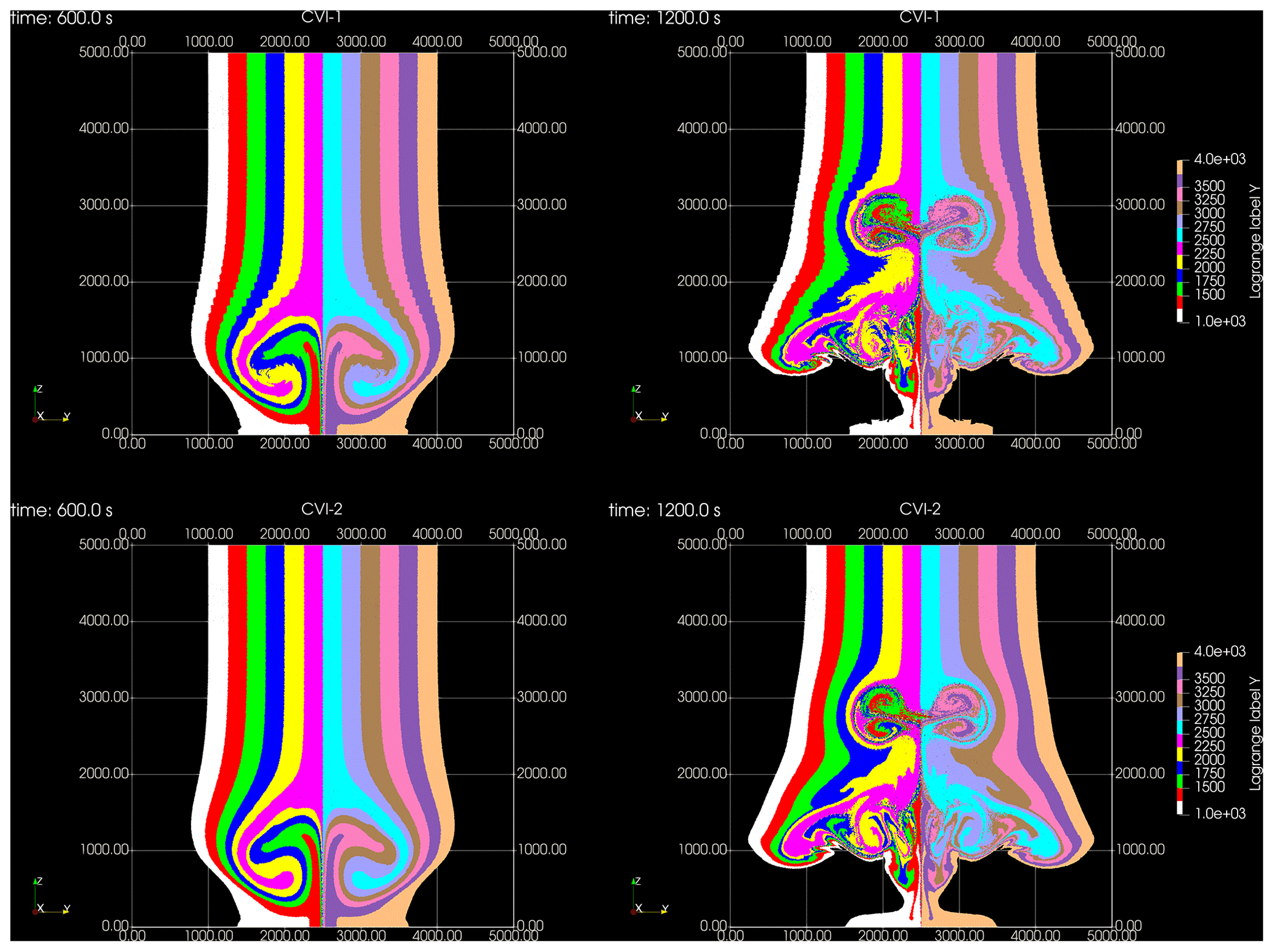
Figure 6Distributions of SD positions at (left) t=600 s and (right) t=1200 s colored by the initial y coordinate (Y) when CVIs of the first-order (CVI-1) and second-order (CVI-2) spatial accuracy are used for SD movement. The ranges of and are shown in each panel.
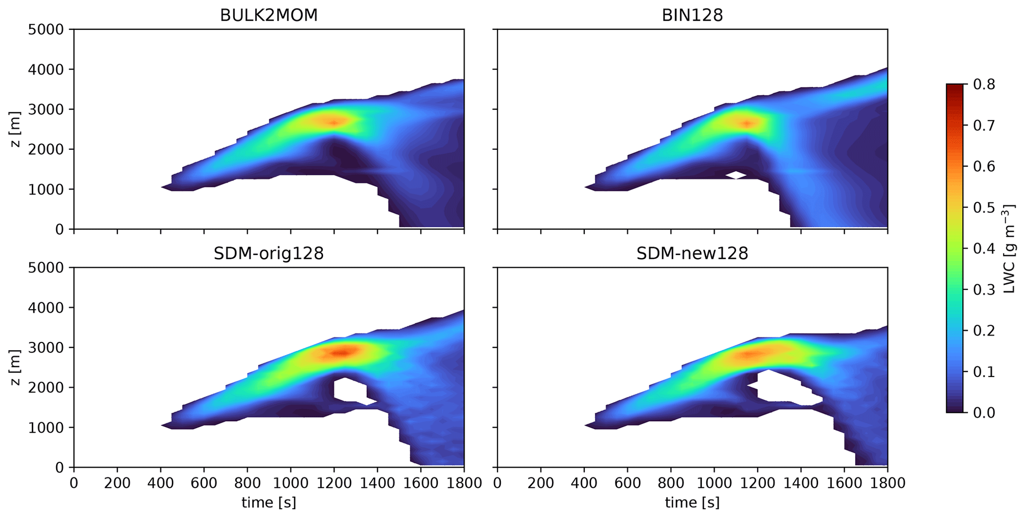
Figure 7Horizontally averaged time–height cross section of the liquid water content (LWC) for different cloud microphysics schemes. Note that only regions with LWC higher than 0.001 g m−3 are shown.
Although we report only the computational performance on FX1000 (A64FX), our innovations are also effective on Intel Xeon. For example, using the Fujitsu Server PRIMERGY GX2570 M6 (CPU part: a theoretical peak performance of 5.53 TFLOPS and memory bandwidth of 409.6 GB s−1) equipped with Intel Xeon Platinum 8360Y, the elapsed time obtained using the two-moment bulk method was 14.0 s, and that obtained using the SDM-new with 128 SDs per cell on average is 13.9 s. The maximum throughput of the SDM-new is 31.6 times that of the two-moment bulk method. The large ratio of the throughput against FX1000 indicates that using FX1000 instead of a more commercial computer with low memory bandwidth (GX2570 M6) is more advantageous for the two-moment bulk method.
Before evaluating the physical performance of SCALE-SDM, we conducted an error analysis of first- and second-order CVI. For this purpose, we analyzed the time evolution of the tracer field following a prescribed 2D Benard-convection-like flow. The error analysis is detailed in the Supplement. By investigating the time evolution of the tracer field with various initial wavenumber patterns, we found that switching from first- to second-order CVI reduced the errors in transient time evolution for any wavenumber and errors following extended simulated times at higher wavenumbers.
Following this, we show the differences in the cloud simulations between the first- and second-order CVI for SD tracking. In the SDM, we can add any new attribute, such as ID, to each SD. By using the ID for analysis, we calculated the initial position of the SD to investigate SD mixing. The distributions of SD positions colored by the initial y coordinate for warm-bubble experiments (SDM-new with 128 SDs per cell on average) are shown in Fig. 6. Buoyancy torque induced by the initial bubble generates vorticity, and the results are different for the case when the first- and second-order CVIs are used. At t=600.0 s, a staircase-like pattern with width approximately equal to the grid length appears in CVI-1 because it does not consider the variation in the velocity component relative to its orthogonal direction within the cell. In contrast, such a pattern does not appear in CVI-2. The motion of the particle in the fluid can be chaotic even for simple flow fields. Particles experience stretching and folding in flows, and fine and complex structures are generated even from large-scale flows. These features are called chaotic mixing (Aref, 1984) from the Lagrangian viewpoint, and they are distinct from turbulence mixing. At t=1200.0 s, fine structure ( m) and filaments (x=1800 m, z=2800 m) appear in CVI-2, whereas such structures are noisy and obscure in CVI-1. This result indicates that such structures in CVI-1 can be nonphysical when assuming that structures in CVI-2 are more correct. The accuracy of the CVI may affect the entrainment and mixing induced by thermal effects, also known as a coherent vortex ring in clouds. Unfortunately, constructing a highly accurate CVI scheme and comparing CVI-1 and CVI-2 with a reference solution requires additional work. Furthermore, the in-cloud flows are generally well-developed turbulent flows, enabling the potential masking of the effect of the numerical accuracy of the CVI by the effect of the subgrid-scale (SGS) turbulence. However, in the meter- to submeter-scale simulations, the moments of the DSD (tracer fields) can highly fluctuate under turbulence, reducing the relative effects of the SGS velocity (LES approach) or viscous diffusion (DNS approach). Consequently, the numerical accuracy of the CVI can affect the time evolutions of cloud microphysics and macrophysics through interactions between eddies and microphysics.
Subsequently, we compared the results of warm-bubble experiments among different cloud microphysics schemes. The horizontally averaged time–height sections of the liquid water content (LWC) are shown in Fig. 7. Here, we denote the names of the experiments, followed by the number of bins and SDs per cell on average, such as SDM-new128, for the results obtained using SDM-new with 128 SDs per cell on average. Here, the elapsed time for the selected cases is SDM-new128 ∼ BULK2MOM < SDM-orig128 < BIN128. In all cases, the qualitative characteristics of time evolution are the same for bubble-induced cloud generation and precipitation pattern. The quantitative characteristics of the time evolution of LWC for t<1000 s are also similar in all cases. The differences between SDM-new and SDM-orig arise when t>1200 s for the precipitation pattern (100 s slower than SDM-orig) and the LWC remains after precipitation in the upper layers (z∼3500 m). However, if the number of SDs is increased to 32 768 (the results are shown in the Supplement) as the differences become small, the differences are mainly attributed to sampling (initialization of the SD number density so that it is proportional to the air density for SDM-new) and randomness (initialization by Sobol sequences, which exhibits faster convergence than a pseudorandom number). The differences in the precipitation and the remaining LWC after precipitation in the upper layers between SDM-new and SDM-orig become small if we disable the improvements presented in this study. Despite some factors indicating differences between SDM-new and SDM-orig, we conclude that their results are similar.
4.3 BOMEX and SCMS cases
In Sect. 4.2, we discussed the evaluation of the computational performance using mainly data throughput by increasing the number of mean SDs per cell. This approach is appropriate for comparing SDM-orig and SDM-new as the contributions of the stencil calculations that are not relevant to the innovations in this study become small. However, the comparison of SDM-new with the two-moment bulk and the bin methods may not be fair. In general, the computational efficiency improves in real-life scenarios when the number of grid points per MPI process is increased. The number of grid points in each MPI process used in Sect. 4.2 was relatively small. In addition, the numerical settings of warm-bubble experiments were too simple to be regarded as representative of real-world problems. Therefore, we also evaluated computational and physical performances for the BOMEX case and a case study of isolated cumulus congestus observed during the Small Cumulus Microphysics Study field campaign (Lasher-Trapp et al., 2005) – this case is referred to as the SCMS case – as they present more practical problems.
The experimental settings for the BOMEX case were based on Siebesma et al. (2003). The computational domain was km for x, y, and z directions, and the horizontal and vertical grid lengths were 50 and 40 m, respectively. The experimental settings for the SCMS case were based on the model intercomparison project for the bin methods and particle-based methods conducted in the International Cloud Modeling Workshop 2021 (see Xue et al., 2022, and references therein). The computational domain was km, and the grid length was 50 m. For both cases, the time interval was Δtdyn=0.1 s, s, and Δtphy=0.2 s. The Rayleigh damping imposed was 500 and 1000 m from the top of the domains for the BOMEX and SCMS cases, respectively. For the two-moment bulk method, we used the mixing scenario parameter m=0.5 for BOMEX and 0.75 for SCMS cases as typical values for the pristine and polluted cases in Jarecka et al. (2013), respectively. In the SDM, SDs were not initially placed in the Rayleigh damping layers, and we did not generate or remove SDs in the regions during simulations. For initialization, the uniform sampling method (i.e., the proposed method using α=1.0) was adopted for both BOMEX and SCMS cases. For the SCMS case, we also used the proposed method using α=0.5 and 0.0 for SDM128 to investigate the sensitivity of cloud microphysical variability to the initialization method.
Ensemble experiments with three members using different initial perturbations controlled by other random seeds were conducted for each experiment. The number of nodes used for simulations was determined as the minimum values so that the memory usage was within the system memory per node. For example, one node of FX1000 was used in both cases for the two-moment bulk method, and one node and two nodes of FX1000 were used in BOMEX and SCMS cases for SDM128, respectively. For time measurement, we used MPI_Wtime but did not use barrier synchronization. During the simulation of three ensemble experiments, we used the normal mode (2.0 GHz, two pipelines), boost mode (2.2 GHz, two pipelines), and boost-eco mode (2.0 GHz, one pipeline) for each ensemble member. We measured the (estimated) energy consumption of entire nodes between measurement intervals.
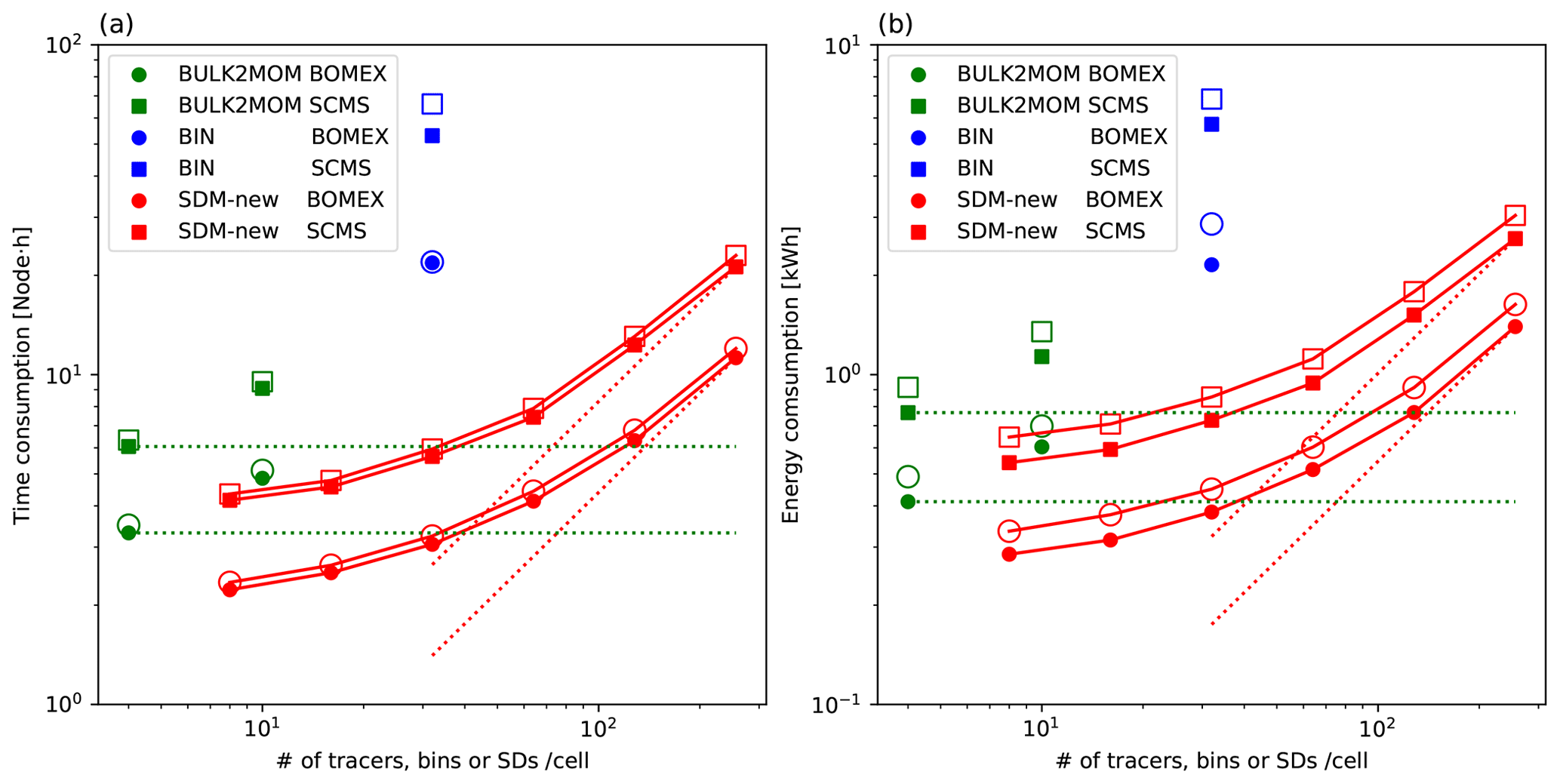
Figure 8Computational resources of BOMEX and SCMS experiments for various cloud microphysics schemes and different numbers of tracers or mean SDs per cell: (a) node hours using normal and boost mode, (b) energy consumption using boost and boost-eco mode. Here, for (a), the results for the boost and normal modes are shown by filled and open markers, respectively. For (b), the results for boost-eco mode and boost mode are shown by filled and open markers, respectively. The dotted red lines show are proportional to the quantities on the horizontal axis.
The computational resources for various cloud microphysics schemes using the normal, boost, and boost-eco modes for each numerical setting are shown in Fig. 8. We first focused on the node hours when the normal mode is used. Here, node hours measure the amount of time for which computing nodes are used, and they are calculated as the product of occupied nodes and the hours. Comparing the results between the SDM with 32 SDs per cell on average (SDM32) and the bin method with 32 bins (BIN32), the node hours of BIN32 are 6.8 times and 11.1 times that of SDM32 for BOMEX and SCMS cases, respectively. The node hours consumed using the SDM with 32 to 64 SDs per cell are comparable to those consumed using the two-moment bulk method; furthermore, they do not increase linearly with increasing number of mean SDs when the number is less than 256. The results are important because we should use more than 128 SDs per cell to obtain converging solutions such as the cloud droplet number concentration with respect to the number of SDs (Shima et al., 2020; Matsushima et al., 2021). In terms of memory usage, the simulations using the two-moment bulk method consumed about 28.5 GB of system memory, whereas those using the SDM with 128 SDs per cell consumed about twice that memory. When the number of available nodes is limited, simulations using the two-moment bulk method can be performed with more grid points.
In Fig. 8, we see that the difference in the patterns among the modes and between panels (a) and (b) is qualitatively small, and the advantage of SDM over the two-moment bulk method and bin method is apparent. For example, the energy consumption of BIN32 is 8.0 times and 6.4 times that of SDM32 for BOMEX and SCMS cases, respectively, when the boost-eco mode is used. In terms of node hours (Fig. 8a), the following relations are observed: boost mode < normal mode. Further, node hours for the boost-eco mode are closer to those for the normal mode (not shown in the figure). For energy consumption (Fig. 8b), the boost-eco mode < boost mode, and the energy consumption by the normal mode is higher than that by the boost-eco mode (not shown in the figure). The results obtained for the boost-eco mode have the best power performance from the viewpoint of computational resources among different modes. Although the boost-eco mode offers an option to improve power performance when FLOPS are not large, the power performances when using not only the two-moment bulk and bin method but also SDM are improved.
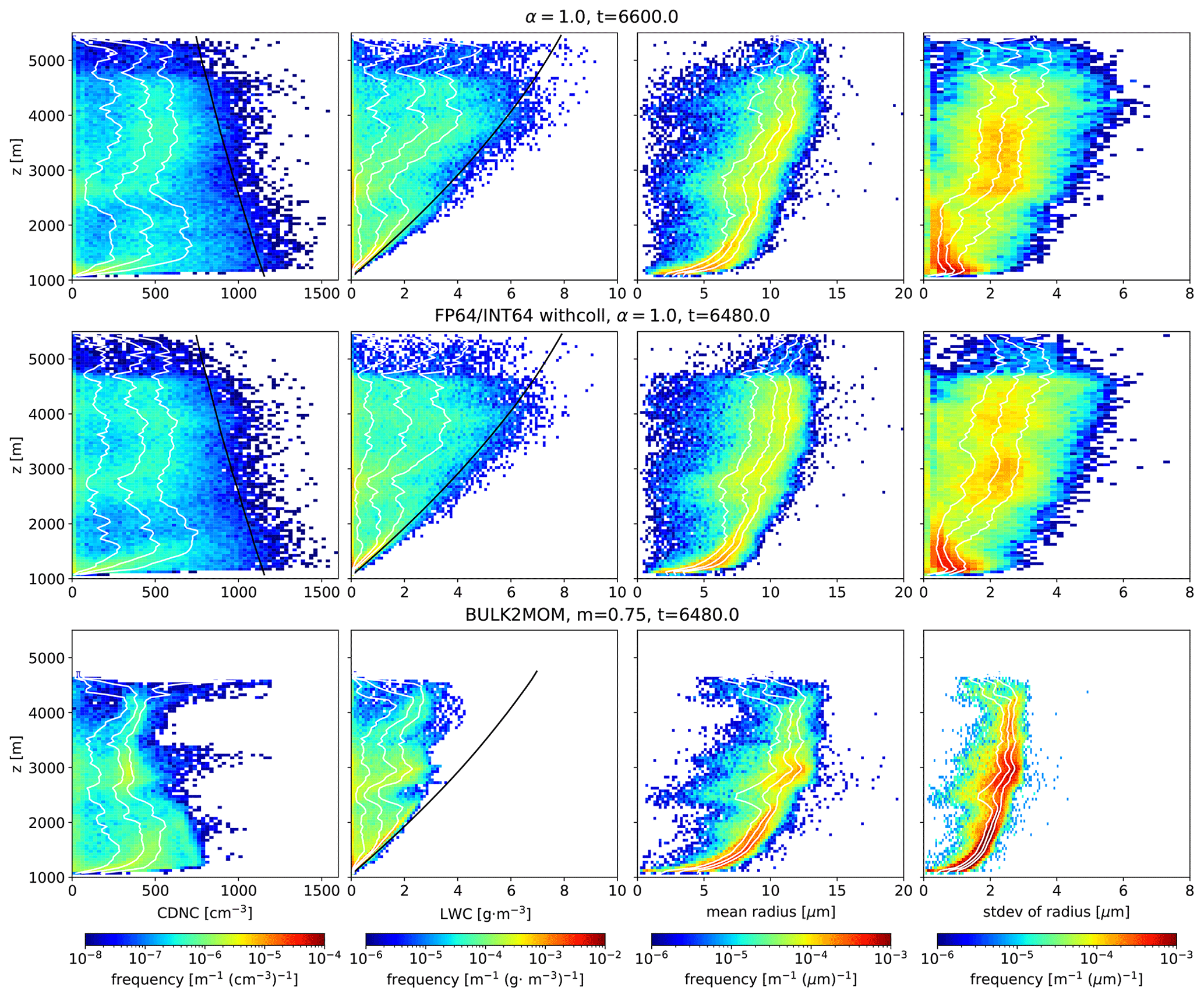
Figure 9Contoured frequency by altitude diagrams (CFADs) of cloud droplet number concentration (CDNC), LWC, and mean and standard deviation of the radius for SCMS experiments. Snapshots are shown of (top row) SDM128 and (middle row) SDM128 obtained using FP64 as floating-point number operations and those with collision–coalescence calculations in all grids and (bottom row) BULK2MOM. In each panel, the quartiles of variables at each height are indicated by white lines. The adiabatic predictions of CDNC and LWC are indicated by black lines in the panels for CDNC and LWC.
We evaluated the physical performance of microphysical spatial variability obtained by the SCMS case experiments. This case is suited for investigating the effect of entrainment and mixing, which may lead to different results among microphysics schemes. In this study, we focused on analyzing the results obtained using the SDM with 128 SDs per cell on average; the computational resources used in this case are about twice as high as those of the two-moment bulk method but smaller than those used for the bin method with 32 bins. The top panel of Fig. 9 shows contoured frequency by altitude diagrams (CFADs) of the cloud droplet number concentration (CDNC), LWC, mean radius, and standard deviation of the radius for one member (α=1.0) of SDM128 at t=6600 s. The selected time of the snapshot was when the cloud-top height almost reached its (local) maximum first (the movie of the CFADs from t=3600 to t=10 800 s is available in the Supplement: SCMS-R50SD128-CFAD-m1.mp4). Once the clouds evolved to have depths larger than approximately ∼3 km, the CFAD patterns did not change much with time qualitatively even for the other ensemble members (in the Supplement: SCMS-R50SD128-CFAD-m[2,3].mp4). To enable intercomparison of models for the readers, each microphysical variable of a cell was calculated by taking statistics for SDs (only) within the cell. However, the spatial scales of the variables were shorter than the scales of effective resolution, which may introduce a numerical influence on the statistics (Matsushima et al., 2021). The adiabatic liquid water content (ALWC) was calculated using Eq. (6) in Eytan et al. (2021), which is recommended for the most accurate comparison with the passive tracer test as a reference solution. In addition, we calculated the adiabatic CDNC. The activated CDNC depends on the updraft of the parcel when crossing the cloud base and hence on the supersaturation of the parcel. However, we simply assign an adiabatic CDNC at the cloud base of 1155 cm−3 as the maximum value assuming large supersaturation, and all haze droplets activate to the cloud droplets. Then, we define an adiabatic CDNC, including the height dependency, as cm−3, where ρa(z) is the air density of the most undiluted cells in the z section, and zcbase is the cloud-base height.
One of the drawbacks of the SDM is the statistical fluctuations caused by finite samples. Indeed, CDNC varies largely centered around 500 cm−3; some samples exceed simple adiabatic prediction, and some samples of LWC also exceed ALWC. However, the frequencies, for which CDNC and LWC are larger than their adiabatic limits, are about 1 order of magnitude smaller than frequencies within adiabatic limits. Near the cloud base, the most frequent values of LWC are close to ALWC. At z=2500 m, the simulated congestus clouds have a kink formed by detrainment, indicating that cloud elements are left behind from the upward flow or moved followed by a downward flow (not shown in figures). The frequency for which LWC ∼0 is large here. Above the middle layer of the clouds (z>2500 m), the LWC is strongly diluted. The mean radius narrowly varies in the lower layers of the clouds, but the variation becomes large above z=2500 m for small droplets because of entrainment and activation. The most frequent values of the standard deviation of the radius decrease as the height increases below z=2500 m in the adiabatic cores of the clouds. Above the middle layers of the clouds, the most frequent values of the standard deviation of the radius remain almost constant or increase with height, and the medians of the frequencies at each height reach 3 µm at the upper layers of the clouds. These features are consistent with typical observations (Arabas et al., 2009). To compare the obtained solution with a reference solution, we also adopted the same experimental setup as that of SDM128 but used mainly FP64. We represent the SD positions in a block by 50 bits using the mapping described in Eq. (6). Meanwhile, we changed the tolerance relative error for Newton iterations in condensation calculations to 10−6 and computed the collision–coalescence process in all grids. Here, the elapsed time and memory usage for only microphysics with FP64 were 1.03(1.45) node hours without (with) collision–coalescence calculations in non-cloudy volumes and 54.9 GB, which are 1.3–1.6 times and 1.8 times larger than the case with FP32 for 0.625(1.14) node hours and 29.7 GB memory usage, respectively. The middle panel of Fig. 9 shows the CFAD analyzed by the reference experiment. Although our innovations include the use of FP32 for the numerical representation of droplet radius, the differences in the patterns of the mean radius between the top and middle panels of Fig. 9 are minor. As we will show in Sect. 6.4.1, simply using FP16 may cause stagnation of the droplet radius and numerical broadening of the DSD for condensational growth, but the use of FP32 does not cause these problems. Therefore, our innovations do not worsen the physical performance compared with the reference solution and typical observation.
The CFAD for the two-moment bulk method is shown in the bottom panel of Fig. 9. The variability of the CDNC and LWC for BULK2MOM is smaller than those for SDM128. As in the SDM128, the mean radius increases with height. The relative standard deviation of the cloud droplet radius for BULK2MOM was analytically calculated to be 0.248 because it prescribes the shape parameters of the generalized gamma distribution. Thus, the mean and standard deviation of the radius have identical patterns except for scaling. The standard deviation of the radius for BULK2MOM is smaller than that for SDM128 and does not decrease as height decreases in the adiabatic core, as seen in the case of SDM128. This happens because the two-moment bulk method cannot represent many possible scenarios inside the clouds due to the empirical assumptions of the DSD. Based on these results, our numerical simulations using new SCALE-SDM provide a qualitatively better solution than that obtained using the two-moment bulk method if twice the computational resources are used by the new SCALE-SDM.
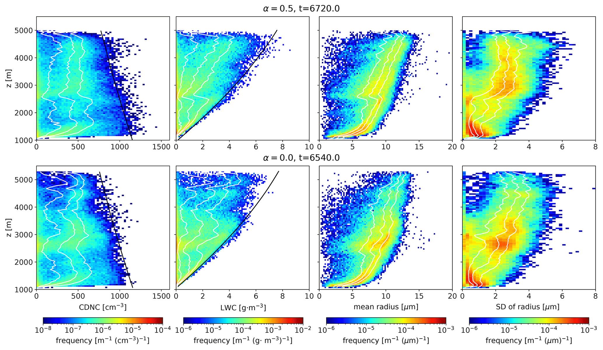
Figure 10CFADs of CDNC, LWC, and the mean and standard deviation of the radius for SCMS experiments using different initialization parameter . In each panel, the quartiles of the variables at each height are shown by white lines. The adiabatic predictions of CDNC and LWC are shown by black lines in the corresponding panels.
In Sect. 3.2, we proposed a new initialization method for meter- to submeter-scale-resolution simulations. Because the aerosol number concentration of the SCMS case is high (11 times that in vanZanten et al., 2011), the importance of collision–coalescence is relatively low. Hence, it may be reasonable to use another initialization parameter instead of α=1.0, which favors faster convergence of collision–coalescence with the number of SDs per cell. Despite the original motivation to develop an initialization method for meter-scale-resolution simulations, we investigated the sensitivity of microphysical variability to α for the SCMS case by 50 m resolution simulations. The CFADs for the initialization parameters α=0.5 and 0.0 are shown in Fig. 10. The selected times of the snapshots are t=6720 and t=6540 s, respectively, which are determined for the same reason as in the case of α=1.0. If we assume no spatial variability of the aerosol number concentrations and that all aerosols (haze droplets) are activated to cloud droplets, the maximum CDNC for the SCMS case is 1155 cm−3. Nevertheless, the maximum values of CDNC reach 1500 cm−3 for α=1.0. As α decreases, the variation in CDNC decreases, and the maximum values of CDNC are almost limited within 1155 cm−3 for α=0.0. These results show that the statistical fluctuation of the aerosol number concentration for large α affects that of the CDNC. We can interpret the cause of the statistical fluctuation of the CDNC as follows. Suppose that for a given supersaturation, the haze droplets that have an aerosol dry radius larger than the specific threshold activate to form cloud droplets, as assumed in the Twomey activation model. Then, the CDNC in each grid cell is determined by the SDs that have an aerosol dry radius larger than the threshold size. If the proposal distribution with a limited area of the support (domain of the random variable) for aerosol dry radius is not similar to the aerosol size distribution, the distribution of the CDNC also has a statistical fluctuation due to the property of importance sampling. Of course, the actual 3D simulations exhibit other effects, such as spatially varying supersaturation, considering a more detailed activation process and the dynamical fluctuation induced by varying the numbers of SDs per cell. On the other hand, the statistical fluctuation of the aerosol mass concentration for small α does not affect that of LWC. Instead, the fluctuations of the LWC decrease as α decreases, and LWC is almost within the ALWC. This finding can be physically interpreted as follows. As α decreases, the samples of small droplets that have a small contribution to the aerosol mass concentration increase, leading to more significant statistical fluctuations of aerosol mass. Similarly, the statistical fluctuation of the LWC for only haze droplets is larger as α decreases (not shown in figures). However, without the turbulence effect, droplet growth by condensation causes the droplet radius of the samples to be more similar with time, thereby damping the statistical fluctuations. In terms of microphysical variability without collision–coalescence, the obtained results for small α are considered to be more accurate because the prediction of the microphysical variable for each grid is less variable. The sensitivity of variability for the mean and standard deviation of the radius to α is unclear. However, the largest values of the mean radius become larger as α increases. This is consistent with the fact that initialization that leads to large dynamic range of multiplicity (larger α in this study) creates larger droplet samples and triggers precipitation, as observed in the study using a box model (Unterstrasser et al., 2017). The results suggest that for nonprecipitating clouds, small α may be allowed even for low-resolution simulations, and optimization of α or proposal distribution by constraints from observations can be explored. For meter- to submeter-scale-resolution simulations, when using small α such that the multiplicity of SDs is not smaller than 1, the microphysical variability induced by condensation–evaporation (majority of the droplets) and precipitation (triggered by rare, lucky droplets) as well as turbulent fluctuations interacting with clouds through phase relaxation can simultaneously better represent the natural variability of clouds.
5.1 Scalability
In Sect. 4, we evaluated the computational and physical performances of SCALE-SDM with relatively low-resolution experiments using at most four nodes. Here, we show the feasibility of using our model for large-scale problems using more computing nodes. First, we show the scaling performance of the new SCALE-SDM for the BOMEX case. Although our numerical model adopts a hybrid type of 3D and 2D domain decompositions using the MPI, we investigated only weak scaling performance in horizontal directions with the vertical domain fixed. This is because almost all clouds localize in the troposphere, and hence extending the vertical domain does not provide any benefit.
For all directions, the grid length is set to 2 m. The number of grid points without halo grids per MPI process is and for the 3D and 2D domain decompositions, respectively. The shape of network topologies is a 3D torus. In one direction of the 3D torus, the 16 MPI processes or nodes are used for vertical domain decomposition. In each node, 2×2 MPI processes per node are used for horizontal domain decomposition. For grid conversions between 3D and 2D domain decompositions, Nz=16 is decomposed by . For the grid system in 2D domain decompositions, grids are divided into groups of for cache blocking. For arithmetic precision, FP64 is used for the dynamical process and mixed precision is used for the SDM. Here, most of the representations and operations for the SDM use FP32/INT32. In contrast, reduction operations, such as calculation of SDs within a cell, to liquid water in the cell use FP64, while calculations of SD cell positions use INT16. The scales of problems per node are mainly limited by memory capacity because the usable system memory of HBM2 is 28 GB, and SD information consumes 8.32 GB memory capacity per node for the above setting if an extra 36 % of the buffer arrays for the SDs is reserved.
The node shapes are , , and with horizontal domains of 1152, 6912, and 13 824 m, respectively. For the BOMEX case, streaks and roll convection with about 1 km wavelength are well resolved for simulations with 12.5 m horizontal and 10 m vertical resolution, and they restrict cloud patterns (Sato et al., 2018). To exclude the effect of domain size, we evaluated the weak scaling performance from the horizontal domain of 1152 m.
Time integrations were performed for 3680 s. The time interval was Δtdyn=0.0046 s, s, and Δtphy=0.0736 s for dynamical process, tracer advection, and physical process, respectively. The short simulated time for the BOMEX case compared with the standard numerical settings is because some challenges remain in outputting large restart files (see Sect. 6.3) and mitigating load imbalance due to clouds. Further, it takes longer to obtain the profiles of the computational performance. However, since the simulated time is sufficiently long for clouds to be generated in the domain and to approach a quasi-steady state, the obtained performance is a good approximation of the actual sustained performance. Note that we set Δtadv smaller than the constraint of the Courant–Friedrichs–Lewy (CFL) condition for tracer advection (typical wind velocity of shear flows is about 10 m s−1 for the BOMEX case). Because the time-splitting method was applied for compressible equations, the noise induced by the acoustic wave is dominant on the tracer fields if Δtadv is larger than several times Δtdyn. If an instantaneous value for dynamical variables is used for the time integration of physical processes and Δtphy is several times Δtdyn, a compressional pattern may arise for the SD density because the instantaneous dynamic variables have a specific phase of the acoustic wave pattern. To reduce these effects, we used dynamic variables averaged over Δtadv for physical process calculations.
For measuring the computational performance, we used both the timer (MPI_Wtime) and fapp. We used the results obtained by the timer only for obtaining a quick view of the elapsed time and that obtained by fapp for other detailed analysis, such as the number of floating-point number operations, number of instructions, and amount of memory transfer. We note that the measured results have an overhead through the use of fapp. The I/O time is included in the total elapsed time of the time integration loops, but it is quite small. We did not use explicit barrier synchronization before and after the time measurement intervals. All-to-all communications with blocking in the local communicator, which consists of Nz MPI processes, were used for converting the grid systems. Since barrier synchronization is not performed for all MPI processes, the effect of wait time for communication will be experienced across dynamics and microphysics processes. However, even if the variations in the presence of clouds in each MPI process are large, these effects become small when the variation of the clouds in each group of Nz MPI processes is small. Since no large-scale cloud organization occurs in this case, we evaluated the computational performance of individual components separately, such as the components of dynamics and microphysics.
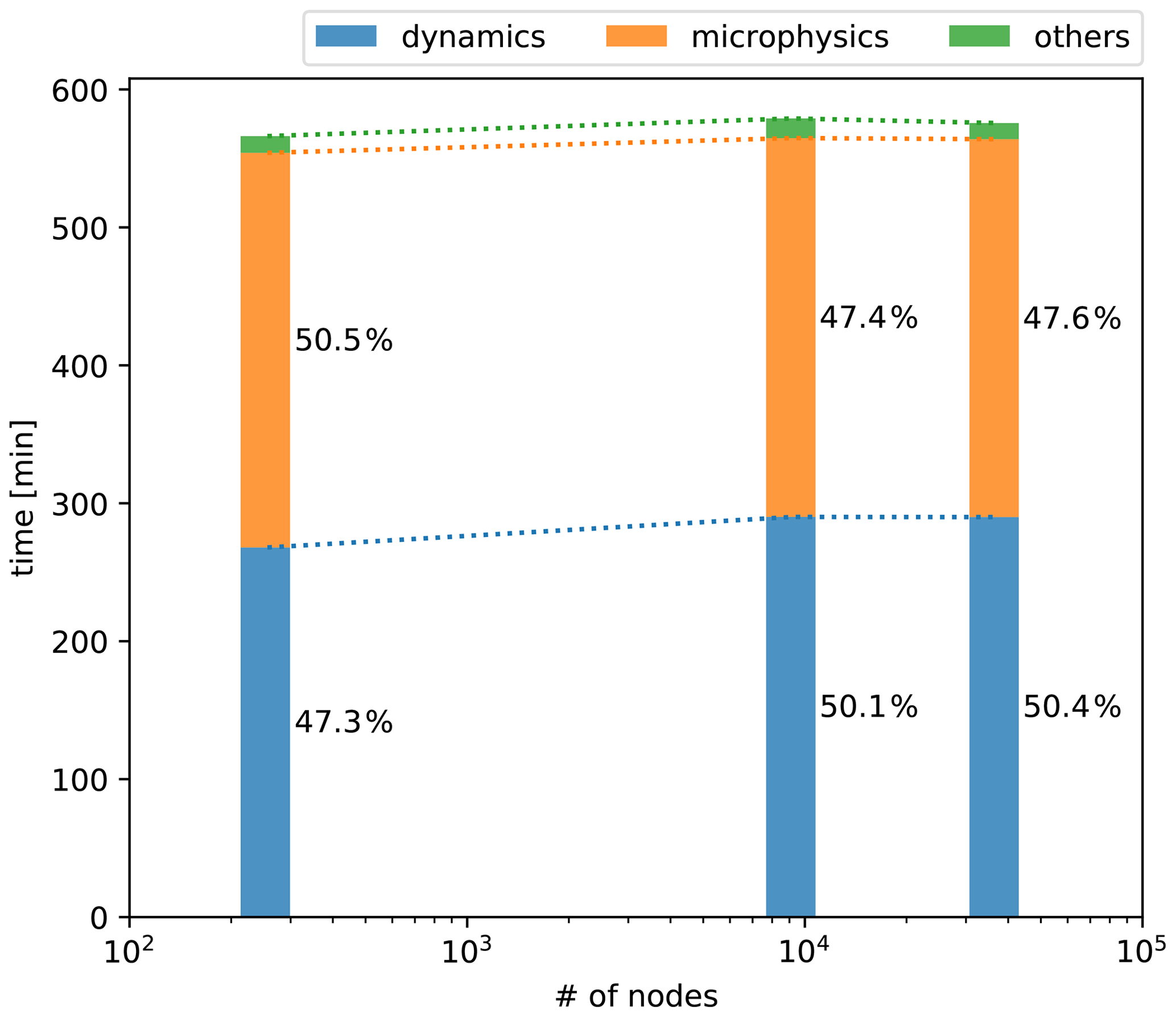
Figure 11Elapsed times corresponding to the dynamics, microphysics, and the other processes for different numbers of nodes.
The weak scaling performance of the new SCALE-SDM obtained for the above settings is shown in Fig. 11. We adopted the grid system for 3D domain decomposition as the default grid system. The elapsed time for the grid system conversion from 3D to 2D or from 2D to 3D domain decomposition is included in the total elapsed time of the process that requires these conversions for calculations. In this case, it is only included in the elapsed time for the microphysics process during the time integration loop. The total elapsed time of the experiments was 566 min for 256 nodes and exhibits 98 % weak scaling for 36 864 nodes. In addition, the elapsed time for dynamics and microphysics was 268 and 286 min for 256 nodes and exhibits 92 % and 104 % weak scaling for 36 864 nodes, respectively. All-to-all communications during the conversion of grid systems do not degrade the weak scaling performance for microphysics because the hop counts of communications are small, and the number of MPI processes involved is small. Other physics processes, such as the turbulence scheme, consume only about 2 % of the total elapsed times.
5.2 Largest-scale problem
The detailed profile of the largest problems among our experiments for the weak scaling test is summarized in Table 3. The peak ratio is obtained against the theoretical peak performance of FP64 operations. The overall time integration loop (excluding the initialization and finalization of the simulation) achieves 7.97 PFLOPS, which is 7.04 % of the theoretical peak performance, and 13.7 PB s−1, which is 37.2 % of the peak performance. The achieved peak ratio of the FLOPS is comparable to that of 6.6 % by NICAM-LETKF (Yashiro et al., 2020), which was nominated for the 2020 Gordon Bell Prize. In addition, because the effective peak ratio of memory throughput performance is approximately >80 % for the STREAM Triad benchmark, the obtained peak ratio achieves about half of it, implying that the overall calculations utilize HBM2 well. At the subprocess level, the short time step (for acoustic waves), which consumes most of the elapsed time in dynamics, achieves 9.5 PFLOPS (8.39 % of the peak) and 21.3 PB s−1 (57.9 %). SD tracking and condensation achieve 15.3 PFLOPS (13.5 % of the peak) and 18.2 PFLOPS (16.1 % of the peak), respectively. These relatively high performances are partly attributed to the use of FP32 for most operations. For these cases, the effective peak ratios for the calculations should be the ratio against peak performance for FP32, which are half of the ratio against FP64 and hence not high. The bottleneck of these processes is a large L1 cache latency of A64FX due to the random access of the grid fields. For collision–coalescence, the peak ratio of the FLOPS is very low. However, in terms of instructions per second (IPS), which includes integer operations, store and load operations, and computation for conditional branches, the performance is not low compared with those of the other processes.
Table 3Elapsed time, FLOPS (peak ratio of the FLOPS, %), peta instructions per second, memory throughput (peak ratio of the memory throughput, %), and particle throughput (no. of floating-point operations per SD).
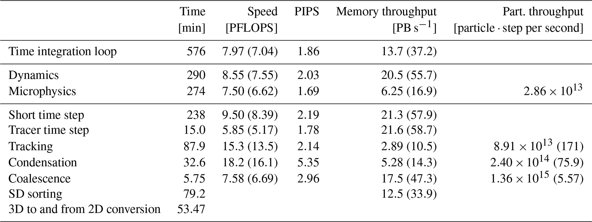
In the SDM, SD tracking, condensation, and collision–coalescence computations consume 44 % of the elapsed time. Elapsed time is also consumed by the data movement time, such as the SD sorting and conversion of grid systems, which still needs improvement. However, it should be noted that the elapsed time may not be the time needed to process SD sorting and conversion of grid systems as load imbalances from other processes will likely affect it. In this experiment, because of the limited memory capacity, we divided loops with a block into small groups to reduce the memory usage for sorting. This affects the increase in the latency and wait time because of synchronization by increasing the communication counts and inefficient OpenMP parallelization by decreasing the loop counts – this is one reason for the long time required for data movement.
The data throughput of the SDM, which we define as shown in Eq. (10) in Sect. 4, as well as the elapsed time, is a fundamental measure that includes not just the number of FLOPs but also all the information about a numerical model, a scheme, an implementation, and a computer. In terms of data throughput, we attempted to compare our results with those of a tokamak plasma PIC simulation, which shares similarities in computational algorithms but has an entirely different target. The tokamak plasma PIC simulation performed by Xiao et al. (2021) was nominated for the 2020 Gordon Bell Prize. It used the entire system of the Sunway OceanLight, which has a higher theoretical peak performance than the Fugaku. For the largest-scale problems, the throughput of the SDM reaches 2.86×10¹³, which is comparable to 3.73×10¹³ particle ⋅ step per second of their study. In addition, the throughput of each subprocess is larger than the simulated throughputs. The major difference between our results and their results in terms of data throughput is the number of operations per particle – it is ∼5000 in their simulations, which is much larger than that achieved in our study. In research focusing on FLOPS as a measure of better computational performance, it is common to reduce the application by increasing the number of FLOPs per particle to fit a computer that has a small , which may result in small data throughput. However, we achieved data throughput comparable to that of their study; moreover, ours is a more practical measure of application than merely considering the FLOPS even if the throughputs are comparable.
Finally, we compare the elapsed time using the SDM with the estimated elapsed time using the two-moment bulk and the bin methods, specifically focusing on the SD movement and tracer advection. These components are chosen because the elapsed time for the microphysics schemes depends on the computational algorithms and degree of optimization, as discussed in Sect. 4.1. However, the elapsed time for tracer advection is more robust in terms of optimization. Moreover, it can be one of the major computational bottlenecks and can be easily estimated. From Table 3, the elapsed time for tracer advection (only water vapor mass mixing ratio) is 15 min and the peak ratio of memory throughput is 58.7 %, which indicates good effective peak performance of tracer advection. In the current implementation, since the time evolution of the tracers was solved by each tracer separately, the total elapsed time for tracer advection was easily estimated as the product of 15 min with the number of tracers. If the water vapor mass mixing ratio plus 4 (10) or 32 tracers is used for the bulk of the bin method, the elapsed time for tracer advection is estimated as 75(165) and 495 min, respectively; these values are larger than the elapsed time of the sum of the SD movement and tracer advection (103 min). For the bin method, the estimated elapsed time of tracer advection is larger than the total elapsed time of the SDM. Here, we explain that this relationship is robust with respect to the optimization of the bin method. The bottleneck of the tracer advection is memory throughput for . We computed the tracer flux in each direction from the mass flux and tracer variables of the previous step to update the tracer variable based on the finite-volume method. If the arrays are large, memory access occurs in nine arrays (one component mass flux, tracer variable, and one component tracer flux for each direction). Since the mass flux is common for different tracer variables and memory access for the tracer variable occurs thrice for computing the tracer flux, our implementation is not optimal for minimizing memory access. Thus, in principle, there is room for optimization. However, since there are no known successful examples of such optimization in the Fugaku (and in the other general-purpose CPUs), tracer advection is a memory-bound application in practice. Then, a possible optimization may be to simply refactor the codes, and we may be able to improve the memory throughput performance of tracer advection to achieve up to 80 % of the theoretical peak performance. However, even with such optimization, the elapsed time of tracer advection with 33 tracers is estimated to be 363 min. Therefore, our simulations with the SDM still have an advantage against the bin method.
6.1 Mixed-phased processes
In this study, we optimized the SDM for only liquid-phase processes. Here, we discuss the possible extensions to incorporate mixed-phase processes into our model.
Shima et al. (2020) extend the SDM approach to consider the morphology of ice particles. Ice processes considered in Shima et al. (2020) include immersion–condensation and homogeneous freezing; melting; deposition and sublimation; and coalescence, riming, and aggregation. To solve these processes, new attributes, such as freezing temperature, equatorial radius, polar radius, and apparent density, are introduced. A critical aspect of the approach using the SDM is that despite many attributes for water and ice particles, the effective number of attributes decreases if particles are in either the water or ice state. For example, when warm and cold processes are considered, the apparent density is necessary for ice particles, but it is not required for liquid droplets. Indeed, the memory space used for the attributes of ice particles can be reused to represent the attributes of droplets when they change to liquids, and vice versa. Thus, if well implemented, the increase in the memory requirement for considering both warm and cold processes can be mitigated. In addition, if we can easily discriminate the particle state as water or ice, the computational cost of the mixed-phase SDM when used for warm clouds will be almost identical to that of the liquid-phase SDM, while computational costs of the bulk method increase due to the new tracers of ice substances and mixed-phase processes (see Figs. 4, 5, and 8).
Alternatively, if water droplets and ice particles are mixed in the cell, computational performance will decrease because of challenges such as the different formats of information on water droplets and ice particles as well as SIMD vectorization. For example, such situations would arise when ice particles grow by riming in a mixed-phase regime of −38 to 0 ∘C for deep convection. In addition, they make assumptions such as particles are in either the water or ice states, and instantaneous melting occurs above 0 ∘C. These problems should be addressed in future works by making fewer assumptions.
6.2 Terrain
An extension of this study to the case with terrain is also essential. For terrain-following coordinates with the map factor used in the regional model, our SD tracking using a fixed-point representation of the SD's position can be applied when we map from terrain-following coordinates to Cartesian coordinates. However, if coordinate mapping is introduced, the CVI scheme may not guarantee consistency between changes in air density and SD density. In addition, there is an additional computational cost for SD tracking. If computational cost is critical, we can include the effect of terrain in the SCALE-SDM by combining it with the immersed boundary or cut-cell methods. Then, the computational performance will not deteriorate because additional cost arises only in the block with the terrain. When realistic terrain is considered, another additional cost will be incurred at the top–bottom–side boundaries to impose inflow–outflow conditions. Moreover, sampling of the initial SDs from the probability distributions normalized by air density will be more complex because the probability distributions will be a 3D distribution. However, the cache-blocking algorithm introduced in this study also helps improve the computational efficiency for such complex processes. Examining if and how we can construct a CVI for terrain-following coordinates and spherical coordinates is a future task.
6.3 Long-time run
In Sect. 5.2, we focused on the feasibility of large-scale problems and performed only about 1 h time integration. To investigate the statistical behavior of clouds, longer time integration is required. However, if we create a checkpoint or restart file for the largest-scale problems in this study, it will require approximately 225 TB without compression for the total number of SDs of 9.39×10¹² SDs, and each SD consists of six attributes with 4 bytes for each attribute. Thus, online analysis becomes imperative if we require information from all SDs. While the output of such a big dataset is feasible on Fugaku, extending the simulated time by enhancing the strong scaling and using numerous nodes will be critical if we plan to increase the number of SDs any further. Alternatively, we may consider the development of lossy compression for SDs, which sacrifices the exact reproducibility of the simulations.
6.4 Can we achieve higher performance?
6.4.1 Lower-precision arithmetic
Since A64FX is a general-purpose CPU with FP16/INT16, it may be possible to reduce memory usage and data movement and achieve higher performance if low-precision arithmetic is utilized. Unfortunately, we could not use it simply for this study. However, since using lower-precision arithmetic may be essential for future high-performance computing, we briefly discuss the obstacles for the same.
Grabowski and Abade (2017) showed that supersaturation fluctuation could broaden the DSD even in the adiabatic parcel. Their method and Abade et al. (2018) serve as a type of parameterization of the turbulence effect for the SDM. Instead of using the 3D numerical model, we discuss the sensitivity of the DSD to numerical precision based on Grabowski and Abade (2017). The numerical settings of the adiabatic parcel model are the same as theirs. The box volume of a parcel is 503 m3. Time integration was performed for 1000 s with the time interval of Δt=0.2 s. In contrast, we used different numerical precisions (FP64, FP32, and FP16) and different rounding modes (round to the nearest mode and two modes of stochastic roundings) for time integration of droplet radius. The detailed mathematical property of stochastic rounding is described in Connolly et al. (2021). Mode 1 rounds to an up/down direction considering the precise position (calculated by other methods such as higher-precision arithmetic) in the interval between the upward and downward rounded values. Mode 2 rounds to an up/down direction with a probability of . For basic operations such as the inner product, the expected values calculated using the stochastic rounding of mode 1 are identical to true values.
The DSDs at 500 and 1000 s are shown in Fig. 12. Without the effect of supersaturation fluctuations, the results obtained using FP64 and FP32 are in good agreement. In contrast, the DSD obtained using FP16 is stagnant in time because the tendency of condensational growth is too small to add to the droplet radius (i.e., loss of trailing digits). However, the DSD obtained using FP16 with mode 1 rounding is similar to that obtained using FP64 or FP32 because the tendencies can be added to the droplet radius stochastically. If we focus on individual SDs, some SDs may experience more rounding down, and some may experience more rounding up. That is, the DSD is slightly diffusive compared with that obtained using FP64 and FP32. If we use FP16 with mode 2, the obtained DSD shifts toward a larger droplet radius (the mean radius reaches about 36 µm at t=1000 s), indicating that the probability for rounding direction is essential to ensure accuracy. With supersaturation fluctuations, the DSD obtained using FP16 is less stagnant because the magnitude of tendencies does not reach 0 because of the fluctuations. The DSD obtained using FP16 with mode 1 is similar to that obtained using FP64 or FP32 except for a slight diffusional trend.
These results indicate that we cannot simply use FP16, but we can use FP16 with mode 1 rounding for some problems. For example, suppose larger Δt is used in low-resolution simulations. In that case, the DSD becomes less diffusive because the effect of rounding becomes small, and the magnitude of supersaturation fluctuations becomes large. On the other hand, if smaller Δt is used in high-resolution simulations, the effect of rounding error on the DSD becomes large. In such cases, the use of FP16 is not suitable even if stochastic rounding is used. For SD movement, because of the variable precision for SD position, it may be feasible to use fixed-point number representation such as INT16 using mode 1 in high-resolution simulations. For collision–coalescence, FP16/INT16 may be troublesome. For example, since the mass of aerosol dissolved in droplets has a wide dynamic range (at least 109 from Fig. 1), it is difficult to represent it with FP16 even if scaling is performed by adopting an appropriate unit.
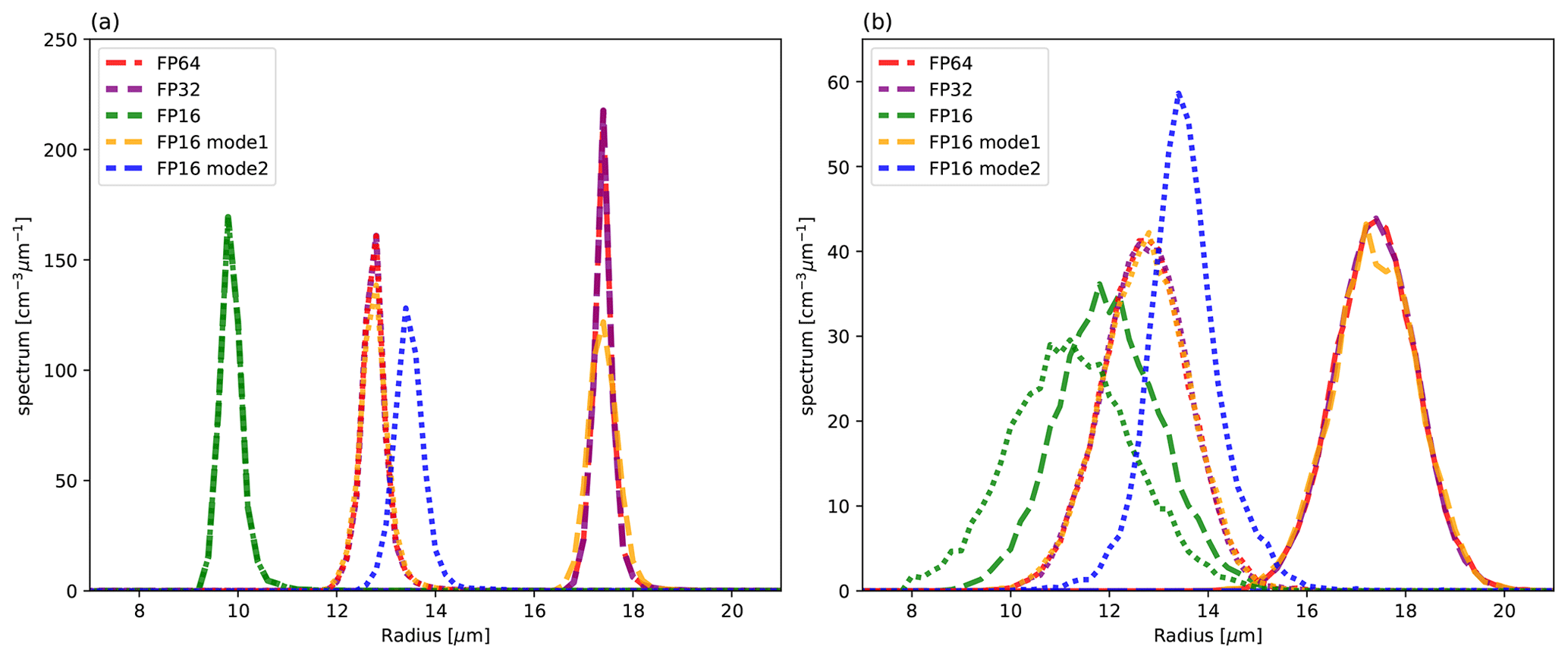
Figure 12DSD obtained using different numerical precisions of floating-point number operations and rounding modes (a) without and (b) with the effect of supersaturation fluctuations. The DSDs for t=500 s and t=1000 s are shown by dotted and dashed lines, respectively.
6.4.2 Reduction of data movement
For the largest-scale problems, the time for data movement (i.e., other than SD tacking, condensation, and collision–coalescence) in the SDM accounts for 53.9 % of the time in the SDM, which accounts for 25.7 % of the total elapsed time. To reduce the time to solution further, it is necessary to optimize data movement.
One possible optimization is to not to sort SDs with a block as a key for every time step of the SDM. Although such an approach is adopted in the tokamak plasma PIC application (Xiao et al., 2021), it requires some consideration for application to the SDM. For collision–coalescence, all SDs in a block must be in the same MPI process to calculate the interaction between SDs in a cell; however, this is not necessary for SD movement and condensation processes. That is, if the for collision–coalescence process can be taken larger than Δtmove for SD movement and Δtcond for condensation, the sorting frequency can be reduced by Δtsort for sorting equal to . In addition, when cloud or rain droplets are not included in a block, the collision–coalescence process is not calculated. Then, it is possible to set Δtsort larger than Δtmove and Δtcond to reduce the sorting frequency.
The second possible optimization is to merge the loops divided by subprocesses in microphysics to lower the required of the SDM. However, this approach may be less effective on computers with high , such as A64FX, and it requires a large amount of L2 cache to store all SD information in a block.
From the operations in each subprocess listed in Table 3, the minimum for the SDM is estimated as , where we assume read–write for six attributes (positions, radius, multiplicity, and aerosol mass) that each consist of 4-byte information. On the other hand, if we separate each subprocess and create a working array for 2-byte SD cell positions instead of using SD positions, the minimum for SD movement and condensation is (assuming read–write for 4-byte three positions and read for 4-byte multiplicity) and (assuming read for 2-byte cell position, read for 4-byte multiplicity and mass of aerosol, and read–write for 4-byte droplet radius), respectively. These results are consistent with the measured (from speed and memory throughput in Table 3) (0.189 and 0.290, respectively). The minimum for SD movement and condensation is smaller than the of the A64FX. However, since the measured for the SDM and collision–coalescence is 0.833 and 2.31, respectively, collision–coalescence is a memory-bound computation, and it causes an increase in the level of the total for the SDM.
As is the case with many computers, the values are expected to be smaller in future. Merging loops will be necessary for future high-performance computing after assuming that high-capacity and high- cache or local memory may be achieved with new technologies such as 3D stacking.
6.5 Possible research directions
Our study focused on optimizing and improving the numerical model. The developed model can be applied to many fields of research from technical and scientific viewpoints.
For model development, in addition to the discussion in Sect. 6.1 to 6.3, the sensitivity of the microphysical variability and precipitation to initialization parameter α should be further explored through meter-scale-resolution simulations. A reduction in the variance of prediction for the SDM, such as when using low-discrepancy sequences, should also be explored. We did not examine this impact in this study. Moreover, the continuation of proposal distributions between the DNS and LES may help in realizing more sophisticated model components. The computational performance of our numerical model may be further improved if we store only the activated cloud and rain droplets in memory, following methods such as those described in Sölch and Kärcher (2010) and Grabowski et al. (2018). Their method can reduce computational cost only when the cloud volume occupies a small fraction of the total volumes and cannot reduce memory usage unless dynamic load balancing is employed. In contrast, our optimization can improve the performance and reduce memory usage even when the cloud volume occupies a large fraction. Suppose we could further reduce the computational cost and data movement for SD tracking. In this case, our model may be more practical than a bulk method in terms of the costs for complex real-world problems because we have already achieved performance comparable to that of a bulk method.
For scientific research, the study enables us to address the problems described in the Introduction as ∼1 m resolution numerical experiments are now possible. For example, we can investigate the cloud turbulence structure in shallow cumulous (Hoffmann et al., 2014) and its interaction with boundary layer turbulence (Sato et al., 2017) in detail. We can also confidently compare the simulation results with observational studies (Matsushima et al., 2021) because the effective resolution of simulations is now comparable to the observational scale (∼10 m). We also improved the initialization method. For stratocumulus, we can investigate the statistical quasi-steady-state DSD, which is affected by cloud-top entrainment and a realistic radiation process.
In the present study, we developed a particle-based cloud model to perform meter- to submeter-scale-resolution simulations to reduce the uncertainty in weather and climate simulations. The super-droplet method (SDM) is promising for complex microphysical process modeling. The main contributions of our SDM-based work are as follows: (1) the development of an initialization method for super-droplets (SDs) that can be used for simulating spatial resolutions between the meter and submeter scales, (2) improvement of the algorithms of the SDM as well as computational and physical performance evaluations, and (3) demonstration of the feasibility for large-scale problems using the supercomputer Fugaku.
-
The uniform sampling method, which has good convergence for the mass of SDs, results in many invalid samples when the number of SDs is larger than the number of real droplets, and multiplicity falls below 1 for rare but important SDs. We developed a new initialization method that is suitable for scales between the meter and submeter scales by connecting the uniform sampling method and constant multiplicity method. The developed initialization method requires a proposal distribution apart from the aerosol distribution. The proposal distribution is formulated as a Fréchet mean with weighting parameter α of proposal distributions between the constant multiplicity and uniform sampling methods. To calculate the mean, we require a measure of the distance between elements. For this metric, instead of using the L2 norm, we suggest using the Wasserstein distance, which is the natural distance between probability distributions. The developed method gives a larger minimum and reduces the dynamic range of SD multiplicity. As α decreases, importance sampling for the aerosol size distribution gradually changes from a variance reduction effect for mass concentration to a variance reduction effect for number concentration.
-
We improved the algorithms of the SDM to achieve high performance on a Fujitsu A64FX processor, which is used in the supercomputer Fugaku. The developed model employs a hybrid type of 3D and 2D domain decomposition using a message passing interface (MPI) to reduce communication cost and load imbalance of calculations for the SDM. The SDM, or more generally the particle-in-cell (PIC) method, has a limitation in high-performance computing because such codes include many complex calculation patterns and conditional branches. We further divided the decomposed domain for the cache block into blocks and set the block size with a spatial scale equivalent to the effective resolution of the large-eddy simulation (LES) so that the variables within the block were nearly uniform. We converted the conditional branches for each SD, which depends on supersaturation or the presence of clouds, into conditional branches for each block. This conversion improved the ratio of identical instructions for each SD and resulted in parallelization by single-instruction multiple-data (SIMD) vectorization even for Newton iterations and reducing the costs of calculations as well as data movement for the collision–coalescence process. For SD movement, the 3D conservative velocity interpolation (CVI) of second-order spatial accuracy on the C-grid was derived to ensure consistency between the changes in SD number density and changes in air density. The interpolated velocity can represent simple vortical and shear flows within a cell, and the divergence at the position of SDs that are calculated from the interpolated velocity is consistent with divergence at the cell. We subtracted partition information using MPI processes and blocks from the information on SD global positions to reduce information per SD. Then, we stored the relative position of the SD in a block with a fixed-point number using FP32. This approach guarantees uniform precision in representing the absolute position of SD across the computational domain and good numerical accuracy for meter- to submeter-resolution simulations, even when using a low-precision format.
Next, we evaluated the computational and physical performances of the model on A64FX by comparing the results obtained using SDM-new, the two-moment bulk method, the bin method, and SDM-orig. Simple warm-bubble experiments showed that the time to solution obtained using SDM-new is smaller than that obtained with the bin method for the same number of tracers or SDs per cell; furthermore, this is comparable to that obtained with the two-moment bulk method when an average of 128 SDs per cell is used. The factors contributing to the enhancements are fewer calculations, higher compactness, and more reasonable use of low-precision arithmetic for SD tracking than for the conventional tracer advection used with the bulk and bin methods. The data throughput of SDM-new is 61.3 times that of SDM-orig. For the Barbados Oceanographic and Meteorological Experiment (BOMEX) and the Small Cumulus Microphysics Study field campaign (SCMS) cases, the computational resources consumed in terms of node hours and energy consumption using the SDM with about 128 SDs per cell are at most twice those consumed using the two-moment bulk method; this is an important result because previous studies showed that the SDM requires about 128 SDs per cell for the convergence of statistics such as the cloud droplet number concentration (CDNC). For the SCMS, new SCALE-SDM yielded realistic microphysical variability comparable with that typically observed in nature, including features that cannot be simulated by the two-moment bulk method. As the initialization parameter α decreased, the in-cloud variabilities of CDNC and liquid water content (LWC) gradually improved, and they were distributed within their simple adiabatic limits. We confirmed that new SCALE-SDM yields qualitatively better solutions than the two-moment bulk method for a comparable time to solution.
-
Finally, we demonstrated the feasibility of using our approach for simulating large-scale problems using the supercomputer Fugaku. The target problem was based on the BOMEX case but with a wider domain and higher spatial resolutions. The new SCALE-SDM exhibited 98 % weak scaling from 256 to 36 864 nodes (23 % of the total system) on Fugaku. For the largest-scale experiment, the horizontal and vertical extents were 13 824 and 3072 m covered with 2 m grids, respectively, and 128 SDs per cell were initialized on average. The time integration was performed for about 1 h. This experiment required about 104 and 442 times the number of grid points and SDs compared to the highest-resolution simulation performed so far (Sato et al., 2018). The overall calculations achieved 7.97 PFLOPS (7.04 % of the peak), and the maximum performance was 18.2 PFLOPS (16.1 % of the peak) for the condensation process in the SDM. The overall throughput in the SDM was 2.86×10¹³ particle ⋅ step per second. These results are comparable to those reported by the recent Gordon Bell Prize finalists, such as the peak ratio of the simulation part of the NICAM-LETKF and the particle throughput of the tokamak plasma PIC simulation. We did not examine the largest-scale problem by using the bin model or the two-moment bulk model; instead, we used a simple extrapolation to estimate that, for the largest problem, the time to simulation of the SDM is shorter than that of the bin method and is comparable to that of the two-moment bulk method.
Several challenges remain – for example, incorporating mixed-phase processes, inclusion of terrain, and long-time integration. However, our approach can handle such further sophistication. The simplification of a loop body innovated in this study can contribute to optimizing the mixed-phase SDM. We also discussed the possibility of reducing attributes, which increases when using mixed-phase SDM, to obtain effective attributes. However, our approach cannot simply be applied to improve the computational performance when the water and ice states are both present in a cell. Thus, further refinement is necessary. The developed CVI scheme can be applied to cases with terrain if we combine our algorithm with the immersed boundary or cut-cell methods. The computational performance of our model will not be degraded in such cases. However, SD tracking over a larger area and in spherical coordinates remains a challenge. The long-time integration of SCALE-SDM is still difficult because of the large data volume. Additional study on reducing data volume by using lossy compression and resampling to restore the data is necessary. For future supercomputers, reducing data movement will be the key to achieving high computational performance. This can be achieved, for example, by reducing information on SD positions, reducing the SD sorting frequency, lowering the application bytes per flops ratio () by merging the loops for physics subprocesses, and developing computers that will make this possible.
Our study is still in the stage of demonstrating the feasibility of large-scale problems for meter- to submeter-scale-resolution simulations. However, suppose the meter-scale-resolution cloud simulations demonstrated in this study can be performed routinely. In this case, these results can be compared with direct numerical simulation (DNS), laboratory experiments, and field studies to study turbulence and microphysics processes over a vast range of scales. Therefore, we strongly believe that our approach is a critical building block of future cloud microphysics models, advances the scientific understanding of clouds, and contributes to reducing the uncertainties of weather simulation and climate projection.
As described in Sect. 3.2, the Wasserstein distance was used to develop a new initialization method for the SDM. The Wasserstein distance and its strongly related optimal transport theory are powerful mathematical tools for tackling problems dealing with a probability distribution, such as machine learning. Here, we briefly introduce the Wasserstein distance, its regularization, and displacement interpolation (McCann, 1997) for readers who are unfamiliar with them.
Let two probability distributions be expressed as a and b. If we allow mass split during transportation, the amount of transportation from ith bin ai to jth bin bj is represented using a coupling matrix Pij. Let a set of coupling matrices U be expressed as
The pth (p≥1) Wasserstein distance Wp for two probability density distributions (a,b) is defined as
That is, is the minimum total cost of transportation from a to b when transport cost from i to j is . On the other hand, the difference between two distributions is often measured using Lp norm:
The significant difference between the Wasserstein distance and Lp norm is that the distance between two distributions is measured in terms of horizontal or vertical differences. Therefore, the Wasserstein distance is a useful measure if the location of the random variable is essential. A coupling matrix P can be obtained by solving a linear programming problem, which is computationally expensive for large-scale problems because its computational complexity is of the order of O(N3) for N dimension. If the computational cost is important, the Sinkhorn distance (Cuturi, 2013), which is a regularization of the Wasserstein distance, can be used instead:
The negative sign of the second term on the right-hand side is the entropy of the probability distribution, which is non-negative and increases with the uncertainty.
For the one-dimensional case, the Wasserstein distance has a simple alternative form:
where and are quantile functions (inverse functions of the cumulative function) for a and b, respectively. In this case, the displacement interpolation (a solution of the continuous case in Eq. 5) is represented as
When we denote right-hand side of Eq. (A6) as
and then Eq. (A6) is rewritten as
Here, we describe a method to obtain y=Fa(x), assuming we already know the specific forms of , and . We change the variable from y to x′ in Eq. (A7) as and we get
This means that if we assign a value to x′, we can obtain a function of x as y=Fa(x). The simple discretization of these calculations yields practical numerical algorithms to obtain y=Fa(x). For example, in this study, we assign b1 as the normalized aerosol distribution and b2 as the uniform distribution. Because b1 is close to 0 near the edge of the support for the distribution and because the quantile function of b1 changes sharply, it is difficult to construct discrete points in y directly. However, if we discretize x′ using equidistant points, the points in y are automatically ensured to resolve the sharp changes in the quantile function.
For simplicity, we considered interpolation within a cell; let the coordinates be and let the regions be , and . Coordinates and velocities are nondimensionalized as follows:
In the following discussion, ′ is omitted, and only the results are shown (the proof is available in Matsushima et al., 2023b).
Let , and be the nondimensional velocities, and let their values on the C-grid be represented as follows:
Further, let the partial differential coefficient for the nondimensional velocities be represented as
Then, the velocity at the SD position obtained using the second-order CVI is represented as follows:
If all partial differential coefficients in Eqs. (B7)–(B12) are set as 0, the interpolated velocity becomes identical to the results obtained using the first-order CVI. The coefficients are evaluated simply by calculating the second-order central difference from the velocities at the cell boundaries.
To solve Eq. (7) numerically, we consider two cases in which the uniqueness of the solution can be easily determined. Here, f is continuous function of R2 in the interval , and it behaves as and . The intermediate value theorem states that Eq. (7) has at least one solution in the interval (0,∞).
To derive the Case 1 condition, we first differentiate f with respect to R2:
Since f′ has a minimum value at where , f′ is always positive in if . In this case, there is one unique solution in the interval. From , we obtain the Case 1 condition of Eq. (8). On the other hand, the solution for f=0 has at most three solutions if , and one or two of them may not be physical solutions. Our purpose is neither to find sufficient conditions for the uniqueness of solutions nor to discriminate physical solutions from at most three solutions. Although Eq. (8) is a more stringent condition than the condition for the uniqueness of solutions, it has the advantage that Newton's method becomes more stable because f′ is always positive.
The Case 2 condition is obtained when we constrain the initial values and environmental conditions. We consider the interval where f behaves as and . The intermediate value theorem states that Eq. (7) has the unique solution in the interval if :
If we give , then . Therefore, the condition is met if . Since b depends on an attribute of the droplets, we can make the condition more stringent to depend on only a variable at a cell. For an unsaturated environment, and .
The numerical model codes and configuration files used in this study are available at https://doi.org/10.5281/zenodo.8103369 (Matsushima et al., 2023a). The supplemental codes, figures, movies, and datasets are available at https://doi.org/10.5281/zenodo.8103378 (Matsushima et al., 2023b).
The supplement related to this article is available online at: https://doi.org/10.5194/gmd-16-6211-2023-supplement.
All authors contributed to conceiving the idea of this study. TM developed the numerical model with assistance from SN and SS, performed numerical experiments, analyzed the results, and drafted the original paper. All authors reviewed and revised the paper and approved the final version for submission.
The contact author has declared that none of the authors has any competing interests.
Publisher's note: Copernicus Publications remains neutral with regard to jurisdictional claims made in the text, published maps, institutional affiliations, or any other geographical representation in this paper. While Copernicus Publications makes every effort to include appropriate place names, the final responsibility lies with the authors.
We thank the two anonymous referees and Simon Unterstrasser for their helpful and constructive comments, which considerably improved our original manuscript. Toshiki Matsushima acknowledges the members of the Center for Planetary Science at Kobe University for encouraging this study. This work was supported by JSPS KAKENHI under grant numbers 20K14559 (Toshiki Matsushima), 19H01974 (Seiya Nishizawa), and 20H00225 and 23H00149 (Shin-ichiro Shima), as well as JST (Moonshot R & D) under grant number JPMJMS2286 (Shin-ichiro Shima). The numerical experiments were conducted using the supercomputer Fugaku (project ID: ra000005) in RIKEN R-CCS, Fujitsu PRIMEHPC FX1000, and PRIMERGY GX2570 (Wisteria/BDEC-01) at the Information Technology Center, University of Tokyo. The authors used facilities of the Center for Cooperative Work on Data Science and Computational Science, University of Hyogo, for data server and analysis. The authors would like to thank Enago (https://www.enago.jp, last access: 24 October 2023) for the English language review on an earlier version of the paper.
This research has been supported by the Japan Society for the Promotion of Science (grant nos. 20K14559, 19H01974, 20H00225, and 23H00149) and the Japan Science and Technology Agency (grant no. JPMJMS2286).
This paper was edited by Simon Unterstrasser and reviewed by two anonymous referees.
Abade, G. C., Grabowski, W. W., and Pawlowska, H.: Broadening of Cloud Droplet Spectra through Eddy Hopping: Turbulent Entraining Parcel Simulations, J. Atmos. Sci., 75, 3365–3379, https://doi.org/10.1175/JAS-D-18-0078.1, 2018. a, b
Akinlabi, E. O., Wacławczyk, M., Mellado, J. P., and Malinowski, S. P.: Estimating turbulence kinetic energy dissipation rates in the numerically simulated stratocumulus cloud-top mixing layer: Evaluation of different methods, J. Atmos. Sci., 76, 1471–1488, https://doi.org/10.1175/JAS-D-18-0146.1, 2019. a
Arabas, S. and Shima, S.-i.: Large-eddy simulations of trade wind cumuli using particle-based microphysics with Monte Carlo coalescence, J. Atmos. Sci., 70, 2768–2777, https://doi.org/10.1175/JAS-D-12-0295.1, 2013. a
Arabas, S. and Shima, S.: On the CCN (de)activation nonlinearities, Nonlin. Processes Geophys., 24, 535–542, https://doi.org/10.5194/npg-24-535-2017, 2017. a
Arabas, S., Pawlowska, H., and Grabowski, W.: Effective radius and droplet spectral width from in-situ aircraft observations in trade-wind cumuli during RICO, Geophys. Res. Lett., 36, L11803, https://doi.org/10.1029/2009GL038257, 2009. a
Arabas, S., Jaruga, A., Pawlowska, H., and Grabowski, W. W.: libcloudph++ 1.0: a single-moment bulk, double-moment bulk, and particle-based warm-rain microphysics library in C++, Geosci. Model Dev., 8, 1677–1707, https://doi.org/10.5194/gmd-8-1677-2015, 2015. a
Aref, H.: Stirring by chaotic advection, J. Fluid Mech., 143, 1–21, https://doi.org/10.1017/S0022112084001233, 1984. a
Bodenschatz, E., Malinowski, S. P., Shaw, R. A., and Stratmann, F.: Can we understand clouds without turbulence?, Science, 327, 970–971, https://doi.org/10.1126/science.1185138, 2010. a
Brenguier, J.-L., Burnet, F., and Geoffroy, O.: Cloud optical thickness and liquid water path – does the k coefficient vary with droplet concentration?, Atmos. Chem. Phys., 11, 9771–9786, https://doi.org/10.5194/acp-11-9771-2011, 2011. a
Brown, A. R., Derbyshire, S., and Mason, P. J.: Large-eddy simulation of stable atmospheric boundary layers with a revised stochastic subgrid model, Q. J. Roy. Meteor. Soc., 120, 1485–1512, https://doi.org/10.1002/qj.49712052004, 1994. a
Chang, K., Bench, J., Brege, M., Cantrell, W., Chandrakar, K., Ciochetto, D., Mazzoleni, C., Mazzoleni, L., Niedermeier, D., and Shaw, R.: A laboratory facility to study gas–aerosol–cloud interactions in a turbulent environment: The Π chamber, B. Am. Meteorol. Soc., 97, 2343–2358, https://doi.org/10.1175/BAMS-D-15-00203.1, 2016. a
Connolly, M. P., Higham, N. J., and Mary, T.: Stochastic rounding and its probabilistic backward error analysis, SIAM J. Sci. Comput., 43, A566–A585, https://doi.org/10.1137/20M1334796, 2021. a, b
Cooper, W. A.: Effects of variable droplet growth histories on droplet size distributions. Part I: Theory, J. Atmos. Sci., 46, 1301–1311, https://doi.org/10.1175/1520-0469(1989)046<1301:EOVDGH>2.0.CO;2, 1989. a
Cuturi, M.: Sinkhorn distances: Lightspeed computation of optimal transport, in: Advances in Neural Information Processing Systems 26 (NIPS 2013), Nevada, US, 5–10 December, 2292–2300, https://proceedings.neurips.cc/paper/2013 (last access: 24 October 2023), 2013. a, b
Decyk, V. K. and Singh, T. V.: Particle-in-cell algorithms for emerging computer architectures, Comput. Phys. Commun., 185, 708–719, https://doi.org/10.1016/j.cpc.2013.10.013, 2014. a
Dziekan, P. and Pawlowska, H.: Stochastic coalescence in Lagrangian cloud microphysics, Atmos. Chem. Phys., 17, 13509–13520, https://doi.org/10.5194/acp-17-13509-2017, 2017. a
Dziekan, P. and Zmijewski, P.: University of Warsaw Lagrangian Cloud Model (UWLCM) 2.0: adaptation of a mixed Eulerian–Lagrangian numerical model for heterogeneous computing clusters, Geosci. Model Dev., 15, 4489–4501, https://doi.org/10.5194/gmd-15-4489-2022, 2022. a, b
Dziekan, P., Waruszewski, M., and Pawlowska, H.: University of Warsaw Lagrangian Cloud Model (UWLCM) 1.0: a modern large-eddy simulation tool for warm cloud modeling with Lagrangian microphysics, Geosci. Model Dev., 12, 2587–2606, https://doi.org/10.5194/gmd-12-2587-2019, 2019. a
Eytan, E., Koren, I., Altaratz, O., Pinsky, M., and Khain, A.: Revisiting adiabatic fraction estimations in cumulus clouds: high-resolution simulations with a passive tracer, Atmos. Chem. Phys., 21, 16203–16217, https://doi.org/10.5194/acp-21-16203-2021, 2021. a
Grabowski, W. W. and Abade, G. C.: Broadening of cloud droplet spectra through eddy hopping: Turbulent adiabatic parcel simulations, J. Atmos. Sci., 74, 1485–1493, https://doi.org/10.1175/JAS-D-17-0043.1, 2017. a, b
Grabowski, W. W. and Jarecka, D.: Modeling condensation in shallow nonprecipitating convection, J. Atmos. Sci., 72, 4661–4679, https://doi.org/10.1175/JAS-D-15-0091.1, 2015. a
Grabowski, W. W. and Wang, L.-P.: Growth of cloud droplets in a turbulent environment, Annu. Rev. Fluid Mech., 45, 293–324, https://doi.org/10.1146/annurev-fluid-011212-140750, 2013. a
Grabowski, W. W., Dziekan, P., and Pawlowska, H.: Lagrangian condensation microphysics with Twomey CCN activation, Geosci. Model Dev., 11, 103–120, https://doi.org/10.5194/gmd-11-103-2018, 2018. a, b, c, d, e, f
Grabowski, W. W., Morrison, H., Shima, S.-i., Abade, G. C., Dziekan, P., and Pawlowska, H.: Modeling of cloud microphysics: Can we do better?, B. Am. Meteorol. Soc., 100, 655–672, https://doi.org/10.1175/BAMS-D-18-0005.1, 2019. a
Grant, R. E., Levenhagen, M., Olivier, S. L., DeBonis, D., Pedretti, K. T., and Laros III, J. H. L.: Standardizing Power Monitoring and Control at Exascale, Computer, 49, 38–46, https://doi.org/10.1109/MC.2016.308, 2016. a
Hoffmann, F.: The effect of spurious cloud edge supersaturations in Lagrangian cloud models: An analytical and numerical study, Mon. Weather Rev., 144, 107–118, https://doi.org/10.1175/MWR-D-15-0234.1, 2016. a, b
Hoffmann, F., Siebert, H., Schumacher, J., Riechelmann, T., Katzwinkel, J., Kumar, B., Götzfried, P., and Raasch, S.: Entrainment and mixing at the interface of shallow cumulus clouds: Results from a combination of observations and simulations, Meteorol. Z., 23, 349–368, https://doi.org/10.1127/0941-2948/2014/0597, 2014. a
Jarecka, D., Grabowski, W. W., Morrison, H., and Pawlowska, H.: Homogeneity of the subgrid-scale turbulent mixing in large-eddy simulation of shallow convection, J. Atmos. Sci., 70, 2751–2767, https://doi.org/10.1175/JAS-D-13-042.1, 2013. a, b, c
Jenny, P., Pope, S. B., Muradoglu, M., and Caughey, D. A.: A hybrid algorithm for the joint PDF equation of turbulent reactive flows, J. Comput. Phys., 166, 218–252, https://doi.org/10.1006/jcph.2000.6646, 2001. a
Lam, M. D., Rothberg, E. E., and Wolf, M. E.: The cache performance and optimizations of blocked algorithms, Oper. Syst. Rev. (ACM), 25, 63–74, https://doi.org/10.1145/106973.106981, 1991. a
Lasher-Trapp, S. G., Cooper, W. A., and Blyth, A. M.: Broadening of droplet size distributions from entrainment and mixing in a cumulus cloud, Q. J. Roy. Meteor. Soc., 131, 195–220, https://doi.org/10.1256/qj.03.199, 2005. a
Matsushima, T., Nishizawa, S., Shima, S.-i., and Grabowski, W.: Intra-cloud Microphysical Variability Obtained from Large-eddy Simulations using the Super-droplet Method, ESS Open Archive [preprint], https://doi.org/10.1002/essoar.10508672.1, 2021. a, b, c
Matsushima, T., Nishizawa, S., and Shima, S.-i.: SCALE-SDM source code and configuration files for meter-to-submeter-scale resolution in cloud simulations, Zenodo [code], https://doi.org/10.5281/zenodo.8103369, 2023a. a
Matsushima, T., Nishizawa, S., and Shima, S.-i.: Supplement to the manuscript “Overcoming computational challenges to realize meter-to-submeter-scale resolution in cloud simulations using super-droplet method” (Matsushima et al., 2023), Zenodo [data set], https://doi.org/10.5281/zenodo.8103378, 2023b. a, b, c
McCann, R. J.: A convexity principle for interacting gases, Adv. Math., 128, 153–179, https://doi.org/10.1006/aima.1997.1634, 1997. a, b
Mellado, J.-P., Bretherton, C., Stevens, B., and Wyant, M.: DNS and LES for simulating stratocumulus: Better together, J. Adv. Model. Earth Sy., 10, 1421–1438, https://doi.org/10.1029/2018MS001312, 2018. a, b, c, d, e, f, g, h, i
Morrison, H. and Grabowski, W. W.: Modeling supersaturation and subgrid-scale mixing with two-moment bulk warm microphysics, J. Atmos. Sci., 65, 792–812, https://doi.org/10.1175/2007JAS2374.1, 2008. a
Morrison, H., van Lier-Walqui, M., Fridlind, A. M., Grabowski, W. W., Harrington, J. Y., Hoose, C., Korolev, A., Kumjian, M. R., Milbrandt, J. A., Pawlowska, H., Posselt, D. J., Prat, O. P., Reimel, K. J., Shima, S.-i., van Diedenhoven, B., and Xue, L.: Confronting the challenge of modeling cloud and precipitation microphysics, J. Adv. Model. Earth Sy., 12, e2019MS001689, https://doi.org/10.1029/2019MS001689, 2020. a
Nakashima, H., Miyake, Y., Usui, H., and Omura, Y.: OhHelp: a scalable domain-decomposing dynamic load balancing for particle-in-cell simulations, in: ICS '09: Proceedings of the 23rd international conference on Supercomputing, NY, USA, 8–12 June, 90–99, https://doi.org/10.1145/1542275.1542293, 2009. a
Nishizawa, S., Yashiro, H., Sato, Y., Miyamoto, Y., and Tomita, H.: Influence of grid aspect ratio on planetary boundary layer turbulence in large-eddy simulations, Geosci. Model Dev., 8, 3393–3419, https://doi.org/10.5194/gmd-8-3393-2015, 2015. a, b
Peyré, G. and Cuturi, M.: Computational optimal transport: With applications to data science, Foundations and Trends® in Machine Learning, 11, 355–607, https://doi.org/10.1561/2200000073, 2019. a
Santambrogio, F.: Optimal transport for applied mathematicians, Birkäuser, Cham, Switzerland, 353 pp., https://doi.org/10.1007/978-3-319-20828-2, 2015. a
Santos, S. P., Caldwell, P. M., and Bretherton, C. S.: Numerically relevant timescales in the MG2 microphysics model, J. Adv. Model. Earth Sy., 12, e2019MS001972, https://doi.org/10.1029/2019MS001972, 2020. a
Sato, Y., Nakajima, T., Suzuki, K., and Iguchi, T.: Application of a Monte Carlo integration method to collision and coagulation growth processes of hydrometeors in a bin-type model, J. Geophys. Res., 114, D09215, https://doi.org/10.1029/2008JD011247, 2009. a, b
Sato, Y., Nishizawa, S., Yashiro, H., Miyamoto, Y., Kajikawa, Y., and Tomita, H.: Impacts of cloud microphysics on trade wind cumulus: which cloud microphysics processes contribute to the diversity in a large eddy simulation?, Prog. Earth Planet Sci., 2, 23, https://doi.org/10.1186/s40645-015-0053-6, 2015. a
Sato, Y., Shima, S.-i., and Tomita, H.: A grid refinement study of trade wind cumuli simulated by a Lagrangian cloud microphysical model: the super-droplet method, Atmos. Sci. Lett., 18, 359–365, https://doi.org/10.1002/asl.764, 2017. a, b, c, d, e, f, g, h, i, j, k
Sato, Y., Shima, S.-i., and Tomita, H.: Numerical Convergence of Shallow Convection Cloud Field Simulations: Comparison Between Double-Moment Eulerian and Particle-Based Lagrangian Microphysics Coupled to the Same Dynamical Core, J. Adv. Model. Earth Sy., 10, 1495–1512, https://doi.org/10.1029/2018MS001285, 2018. a, b, c, d
Schmitz, M. A., Heitz, M., Bonneel, N., Ngole, F., Coeurjolly, D., Cuturi, M., Peyré, G., and Starck, J.-L.: Wasserstein dictionary learning: Optimal transport-based unsupervised nonlinear dictionary learning, SIAM J. Imaging Sci., 11, 643–678, https://doi.org/10.1137/17M1140431, 2018. a
Schulz, B. and Mellado, J. P.: Competing effects of droplet sedimentation and wind shear on entrainment in stratocumulus, J. Adv. Model. Earth Sy., 11, 1830–1846, https://doi.org/10.1029/2019MS001617, 2019. a, b
Seifert, A. and Rasp, S.: Potential and limitations of machine learning for modeling warm-rain cloud microphysical processes, J. Adv. Model. Earth Sy., 12, e2020MS002301, https://doi.org/10.1029/2020MS002301, 2020. a
Seiki, T. and Nakajima, T.: Aerosol effects of the condensation process on a convective cloud simulation, J. Atmos. Sci., 71, 833–853, https://doi.org/10.1175/JAS-D-12-0195.1, 2014. a, b, c, d, e
Shaw, R. A., Cantrell, W., Chen, S., Chuang, P., Donahue, N., Feingold, G., Kollias, P., Korolev, A., Kreidenweis, S., Krueger, S., Mellado, J. P., Niedermeier, D., and Xue, L.: Cloud–aerosol–turbulence interactions: Science priorities and concepts for a large-scale laboratory facility, B. Am. Meteorol. Soc., 101, E1026–E1035, https://doi.org/10.1175/BAMS-D-20-0009.1, 2020. a
Shima, S., Sato, Y., Hashimoto, A., and Misumi, R.: Predicting the morphology of ice particles in deep convection using the super-droplet method: development and evaluation of SCALE-SDM 0.2.5-2.2.0, -2.2.1, and -2.2.2, Geosci. Model Dev., 13, 4107–4157, https://doi.org/10.5194/gmd-13-4107-2020, 2020. a, b, c, d, e, f, g, h
Shima, S.-i., Kusano, K., Kawano, A., Sugiyama, T., and Kawahara, S.: The super-droplet method for the numerical simulation of clouds and precipitation: A particle-based and probabilistic microphysics model coupled with a non-hydrostatic model, Q. J. Roy. Meteor. Soc., 135, 1307–1320, https://doi.org/10.1002/qj.441, 2009. a, b, c, d, e, f
Siebesma, A. P., Bretherton, C. S., Brown, A., Chlond, A., Cuxart, J., Duynkerke, P. G., Jiang, H., Khairoutdinov, M., Lewellen, D., Moeng, C.-H., Sanchez, E., Stevens, B., and Stevens, D. E.: A large eddy simulation intercomparison study of shallow cumulus convection, J. Atmos. Sci., 60, 1201–1219, https://doi.org/10.1175/1520-0469(2003)60<1201:ALESIS>2.0.CO;2, 2003. a, b
Skamarock, W. C.: Evaluating mesoscale NWP models using kinetic energy spectra, Mon. Weather Rev., 132, 3019–3032, https://doi.org/10.1175/MWR2830.1, 2004. a
Sölch, I. and Kärcher, B.: A large-eddy model for cirrus clouds with explicit aerosol and ice microphysics and Lagrangian ice particle tracking, Q. J. Roy. Meteor. Soc., 136, 2074–2093, https://doi.org/10.1002/qj.689, 2010. a
Stevens, B., Moeng, C.-H., Ackerman, A. S., Bretherton, C. S., Chlond, A., de Roode, S., Edwards, J., Golaz, J.-C., Jiang, H., Khairoutdinov, M., Kirkpatrick, M. P., Lewellen, D. C., Lock, A., Müller, F., Stevens, D. E., Whelan, E., and Zhu, P.: Evaluation of large-eddy simulations via observations of nocturnal marine stratocumulus, Mon. Weather Rev., 133, 1443–1462, https://doi.org/10.1175/MWR2930.1, 2005. a, b
Suzuki, K., Nakajima, T., Nakajima, T. Y., and Khain, A. P.: A study of microphysical mechanisms for correlation patterns between droplet radius and optical thickness of warm clouds with a spectral bin microphysics cloud model, J. Atmos. Sci., 67, 1126–1141, https://doi.org/10.1175/2009JAS3283.1, 2010. a, b, c
Tong, M. and Xue, M.: Simultaneous estimation of microphysical parameters and atmospheric state with simulated radar data and ensemble square root Kalman filter. Part II: Parameter estimation experiments, Mon. Weather Rev., 136, 1649–1668, https://doi.org/10.1175/2007MWR2071.1, 2008. a
Unterstrasser, S. and Sölch, I.: Optimisation of the simulation particle number in a Lagrangian ice microphysical model, Geosci. Model Dev., 7, 695–709, https://doi.org/10.5194/gmd-7-695-2014, 2014. a
Unterstrasser, S., Hoffmann, F., and Lerch, M.: Collection/aggregation algorithms in Lagrangian cloud microphysical models: rigorous evaluation in box model simulations, Geosci. Model Dev., 10, 1521–1548, https://doi.org/10.5194/gmd-10-1521-2017, 2017. a, b, c, d
Unterstrasser, S., Hoffmann, F., and Lerch, M.: Collisional growth in a particle-based cloud microphysical model: insights from column model simulations using LCM1D (v1.0), Geosci. Model Dev., 13, 5119–5145, https://doi.org/10.5194/gmd-13-5119-2020, 2020. a
vanZanten, M. C., Stevens, B., Nuijens, L., Siebesma, A. P., Ackerman, A. S., Burnet, F., Cheng, A., Couvreux, F., Jiang, H., Khairoutdinov, M., Kogan, Y., Lewellen, D. C., Mechem, D., Nakamura, K., Noda, A., Shipway, B. J., Slawinska, J., Wang, S., and Wyszogrodzki, A.: Controls on precipitation and cloudiness in simulations of trade-wind cumulus as observed during RICO, J. Adv. Model. Earth Sy., 3, M06001, https://doi.org/10.1029/2011MS000056, 2011. a, b, c, d
Wang, H., Agrusta, R., and van Hunen, J.: Advantages of a conservative velocity interpolation (CVI) scheme for particle-in-cell methods with application in geodynamic modeling, Geochem. Geophy. Geosy., 16, 2015–2023, https://doi.org/10.1002/2015GC005824, 2015. a
Wicker, L. J. and Skamarock, W. C.: Time-splitting methods for elastic models using forward time schemes, Mon. Weather Rev., 130, 2088–2097, https://doi.org/10.1175/1520-0493(2002)130<2088:TSMFEM>2.0.CO;2, 2002. a
Xiao, J., Chen, J., Zheng, J., An, H., Huang, S., Yang, C., Li, F., Zhang, Z., Huang, Y., Han, W., Liu, X., Chen, D., Liu, Z., Zhuang, G., Chen, J., Li, G., Sun, X., and Chen, Q.: Symplectic structure-preserving particle-in-cell whole-volume simulation of tokamak plasmas to 111.3 trillion particles and 25.7 billion grids, in: SC '21: International Conference for High Performance Computing, Networking, Storage and Analysis, St. Louis, Missouri, USA, 14–19 November, 1–13, https://doi.org/10.1145/3458817.3487398, 2021. a, b
Xue, L., Bera, S., Chen, S., Choudhary, H., Dixit, S., Grabowski, W. W., Jayakumar, S., Krueger, S., Kulkarni, G., Lasher-Trapp, S., Mallinson, H., Prabhakaran, T., and Shima, S.-i.: Progress and Challenges in Modeling Dynamics–Microphysics Interactions: From the Pi Chamber to Monsoon Convection, B. Am. Meteorol. Soc., 103, E1413–E1420, https://doi.org/10.1175/BAMS-D-22-0018.1, 2022. a
Yashiro, H., Terasaki, K., Kawai, Y., Kudo, S., Miyoshi, T., Imamura, T., Minami, K., Inoue, H., Nishiki, T., Saji, T., Satoh, M., and Tomita, H.: A 1024-member ensemble data assimilation with 3.5-km mesh global weather simulations, in: SC '20: International Conference for High Performance Computing, Networking, Storage and Analysis, IEEE, Atlanta, GA, USA, 9–19 November, 1–10, https://doi.org/10.1109/SC41405.2020.00005, 2020. a
Zalesak, S. T.: Fully multidimensional flux-corrected transport algorithms for fluids, J. Comput. Phys., 31, 335–362, https://doi.org/10.1016/0021-9991(79)90051-2, 1979. a
- Abstract
- Introduction
- Overview of the problem
- Numerical model
- Comparison of model performance
- Applicability for large-scale problems
- Discussion
- Conclusions
- Appendix A: Wasserstein distance
- Appendix B: Second-order conservative velocity interpolation on Arakawa C-grid
- Appendix C: Conditions for existence and uniqueness of the solutions of discretized activation–condensation equation
- Code and data availability
- Author contributions
- Competing interests
- Disclaimer
- Acknowledgements
- Financial support
- Review statement
- References
- Supplement