Simulated stable water isotopes during the mid-Holocene and pre-industrial periods using AWI-ESM-2.1-wiso

Numerical simulations employing prognostic stable water isotopes can not only facilitate our understanding of hydrological processes and climate change but also allow for a direct comparison between isotope signals obtained from models and various archives. In the current work, we describe the performance and explore the potential of a new version of the Earth system model AWI-ESM (Alfred Wegener Institute Earth System Model), labeled AWI-ESM-2.1-wiso, in which we incorporated three isotope tracers into all relevant components of the water cycle. We present here the results of pre-industrial (PI) and mid-Holocene (MH) simulations. The model reproduces the observed PI isotope compositions in both precipitation and seawater well and captures their major differences from the MH conditions. The simulated relationship between the isotope composition in precipitation (δ¹⁸O_p) and surface air temperature is very similar between the PI and MH conditions, and it is largely consistent with modern observations despite some regional model biases. The ratio of the MH–PI difference in δ¹⁸O_p to the MH–PI difference in surface air temperature is comparable to proxy records over Greenland and Antarctica only when summertime air temperature is considered. An amount effect is evident over the North African monsoon domain, where a negative correlation between δ¹⁸O_p and the amount of precipitation is simulated. As an example of model applications, we studied the onset and withdrawal date of the MH West African summer monsoon (WASM) using daily variables. We find that defining the WASM onset based on precipitation alone may yield erroneous results due to the substantial daily variations in precipitation, which may obscure the distinction between pre-monsoon and monsoon seasons. Combining precipitation and isotope indicators, we suggest in this work a novel method for identifying the commencement of the WASM. Moreover, we do not find an obvious difference between the MH and PI periods in terms of the mean onset of the WASM. However, an advancement in the WASM withdrawal is found in the MH compared to the PI period due to an earlier decline in insolation over the northern location of Intertropical Convergence Zone (ITCZ).

1 Introduction

Stable water isotopologues (in this study H${}_{\mathrm{2}}^{\mathrm{16}}$O, H${}_{\mathrm{2}}^{\mathrm{18}}$O, and HD¹⁶O, hereafter called stable water isotopes) are natural tracers in the water cycle and can serve as valuable indicators of climate change (Dansgaard, 1964). The compositions of stable water isotopes are commonly expressed as delta values in terms of permil (‰) deviation from a standard, e.g., the Vienna Standard Mean Ocean Water (V-SMOW). Various syntheses of water isotope measurements have arisen during the last decades, for example the Global Network of Isotopes in Precipitation (GNIP) (Schotterer et al., 1996; IAEA, 2018) and the global oxygen-18 database of seawater from the Goddard Institute for Space Studies (GISS) (Bigg and Rohling, 2000; Schmidt et al., 2023). These datasets facilitate a greater comprehension of the current hydrological cycle and associated climate processes. In addition, numerous attempts have been undertaken to interpret past climate changes from a variety of stable water isotope archives, such as the polar ice cores (e.g., North, 2004; Petit et al., 1999), tropical ice cores (e.g., Thompson et al., 1995, 1994), subtropical speleothems (e.g., Ku and Li, 1998; Fleitmann et al., 2004), and planktonic and benthic foraminifera (e.g., Shackleton et al., 1983; McManus et al., 1999). The translation from isotopic records to past climate fluctuations is commonly carried out by using the observed modern spatial slope between isotope composition and physical variables (e.g., temperature, salinity of the seawater) as a surrogate for the temporal slope of the past. Typical examples include the reconstruction of Antarctic temperature at glacial–interglacial timescales based on isotope records from Antarctic ice cores (Petit et al., 1999; EPICA community members, 2004; Jouzel et al., 2007; Kawamura et al., 2007), as well as the reconstruction of the Northern Hemisphere temperature from Greenland ice core measurements (North, 2004; Thomas et al., 2007; Guillevic et al., 2013; Buizert et al., 2014). Moreover, isotopic ratios documented in subtropical speleothems can reflect past monsoon rainfall variability with a high temporal resolution (Johnson et al., 2006; Maher, 2008).

The observed present-day spatial slope between isotope and temperature is widely used as a surrogate for the temporal gradient at reconstruction sites (Cuffey et al., 1992; Sime et al., 2009; Kindler et al., 2014). A model simulation using isoCAM3 suggests that both the temporal slope and spatial slope remain largely stable throughout the last deglaciation (Guan et al., 2016). However, a significant regional dependency is found for both the temporal slope (Guan et al., 2016) and the spatial slope (Sjolte et al., 2011). Guan et al. (2016) also point out that the temporal slope is usually smaller than the spatial slope in the extratropics. Besides, some studies indicate that the temporal relationship between isotopes and temperature may vary over time and that the temporal isotope–temperature slope may differ from the observed spatial slope in the present day (e.g., Werner et al., 2000; Sjolte et al., 2014). Therefore, using isotope data from different archives to draw quantitative inferences about past climate variability remains challenging. In addition, the isotope-based temperature reconstruction over Greenland during the Last Glacial Maximum (LGM) is prone to biases due to changes in the seasonality of precipitation (e.g., Werner et al., 2000). Changes in the primary moisture source areas or air mass transport trajectories during the LGM can have a significant impact on the isotope–temperature relationship, which has the potential to invalidate the isotopic paleothermometer approach based on the use of modern observations (Delaygue et al., 2000b; Werner et al., 2001). Moreover, the isotope–temperature relationship can also be influenced by the proportion of continental sources and recycling of vapor under interglacial boundary conditions (Sjolte et al., 2014). During the last deglaciation, the temporal slope between δ¹⁸O and temperature over Greenland has been found to be much lower than the spatial slope obtained from modern measurements (Guillevic et al., 2013; Buizert et al., 2014). Evidence from previous studies has shown a heterogeneous isotope–temperature relationship in the East Antarctic plateau during interglacial periods (Sime et al., 2009; Cauquoin et al., 2015). Over subtropical continents, the isotopic signature in speleothems has often been used as an indicator for the intensity of monsoon rainfall; however, this isotopic signal is sensitive to a number of other variables, including local temperature, specific humidity, and atmospheric circulation (Lachniet, 2009). Therefore, it is possible that the isotopic composition determined from subtropical speleothems does not exclusively represent the local precipitation rate.

Over the past few decades, isotope-enabled models have evolved as valuable, well-established tools, improving our understanding of the relationship between water isotopes and climate variables. Explicitly, the water isotopes H${}_{\mathrm{2}}^{\mathrm{18}}$O and HDO have been incorporated into relevant components of the hydrological cycle in atmospheric general circulation models (GCMs) (Joussaume et al., 1984; Jouzel et al., 1987; Hoffmann et al., 1998; Mathieu et al., 2002; Schmidt et al., 2005; Lee et al., 2007; Risi et al., 2010; Werner et al., 2011; Nusbaumer et al., 2017; Okazaki and Yoshimura, 2019), oceanic GCMs (Schmidt, 1998; Paul et al., 1999; Delaygue et al., 2000a; Wadley et al., 2002; Xu et al., 2012; Liu et al., 2014), land surface models (Riley and Berry, 2002; Fischer, 2006; Yoshimura et al., 2006; Haese et al., 2013), and coupled Earth system models (Roche et al., 2004; Schmidt et al., 2007; Tindall et al., 2009; Brennan et al., 2012; Roche and Caley, 2013; Werner et al., 2016; Cauquoin et al., 2019; Brady et al., 2019). They can be used to simulate in parallel the isotopic and climatic signals of the past. More importantly, isotope-enabled models permit a direct comparison between isotopic measurements and model simulations and offer the opportunity to comprehend the underlying mechanisms responsible for the variations in isotopic composition documented in various archives (Werner et al., 2000; Risi et al., 2012; Phipps et al., 2013; Bühler et al., 2022).

The mid-Holocene (MH, around 6 ka) is one of the foci of the Paleoclimate Model Intercomparison Project (PMIP) (Kageyama et al., 2018) and has drawn considerable interest from paleoclimate researchers (Yin and Berger, 2015; Brierley et al., 2020; Otto-Bliesner et al., 2021). Proxy-based reconstructions of global temperature have shown a Holocene thermal maximum (HTM) possibly centered around the MH (Kaufman et al., 2020). However, a recent study emphasizes a spatial heterogeneity of Holocene temperature trends, in contrast to the concept of a globally synchronous MH thermal optimum (Cartapanis et al., 2022). Important external forcings that differ between the MH and today include the Earth's orbital parameters and greenhouse gas concentrations (Berger, 1977; Köhler et al., 2017). As a result of the changes in orbital parameters, during the MH, solar insolation was higher in the boreal summer and lower in the boreal winter than it is today, resulting in an enhanced seasonal cycle (Kukla et al., 2002; Shi and Lohmann, 2016; Shi et al., 2020; Zhang et al., 2021). Moreover, the greenhouse gas concentration during the MH was lower than today, which caused a modest global cooling superimposed on the orbital effect (Brierley et al., 2020).

Previous studies identified increased Northern Hemisphere monsoonal precipitation on the basis of model simulations (Jiang et al., 2015; Braconnot et al., 2007; Nikolova et al., 2013; Fischer and Jungclaus, 2010) and various proxy records (Wang et al., 2008b; Bartlein et al., 2011). Due to the intensification in rainfall, the isotopic composition of precipitation decreases over North Africa and South Asia (Cauquoin et al., 2019). Over Greenland, both model simulation and ice core measurements show an enriched δ¹⁸O in precipitation associated with an increase in annual mean temperature during the MH (Cauquoin et al., 2019; North, 2004). Most climate models participating in the PMIP4 simulate an enhanced Northern Hemisphere summer monsoon during the MH periods relative to the present day (D'Agostino et al., 2019). Further evidence of this is also documented in pollen-based proxy records (Bartlein et al., 2011). The subtropical rainfall was isotopically more depleted (Herold and Lohmann, 2009; Cauquoin et al., 2019; Gierz et al., 2017) as a result of enhanced precipitation and stronger advection of moisture from the source ocean surface (Herold and Lohmann, 2009). A variety of studies have attempted to derive the modern summer monsoon onset based on observations for the regions of Asia (Nguyen-Le et al., 2014; Moron and Robertson, 2014; Joseph et al., 2006), Africa (Sultan and Janicot, 2003; Fitzpatrick et al., 2015; Dunning et al., 2016), and North America (Bombardi et al., 2020). However, because proxy time series cannot resolve daily variations in precipitation or water isotopes, there is a lack of knowledge on the initiation date of the MH summer monsoon due to low temporal resolution in proxy data. Since models can give adequate high-frequency variables to explore synoptic phenomena, we can study the possible characteristics of monsoon onset using the model outputs with high temporal resolution under both pre-industrial (PI) and MH climatic conditions.

In the present study, we put our focus on three major aspects: first, we have developed a new Earth system model with enabled stable water diagnostics, called hereafter AWI-ESM-2.1-wiso (Alfred Wegener Institute Earth System Model with isotope). This model inherits the atmosphere and land surface components from MPI-ESM-wiso (Max Planck Institute) (Cauquoin et al., 2019). We additionally implemented three isotopic tracers (i.e., H${}_{\mathrm{2}}^{\mathrm{16}}$O, H${}_{\mathrm{2}}^{\mathrm{18}}$O, and HDO) into the ice–ocean module FESOM2 (Danilov et al., 2017), all of which are treated as passive tracers in the ocean, in the same way as in the oceanic component of MPI-ESM-wiso (i.e., MPIOM). Compared to MPIOM, FESOM2 has the advantage of adopting a much higher spatial resolution in the region of interest (Fig. S1). Second, we provide the preliminary results of AWI-ESM-2.1-wiso simulations under both PI and MH boundary conditions, with an emphasis on the global distribution of isotope compositions and the relationship between water isotopes and the climatic variables during both time periods. We aim to give insight into the MH with the use of a state-of-the-art high-resolution Earth system model with the capability of simulating isotopic compositions in all relevant hydrological components. Finally, with the utility of model outputs at daily frequency, we analyze the initiation date of the West African summer monsoon onset in the PI and MH eras.

2 Methodology

2.1 Model component description

Stable water isotopes have been incorporated into all relevant components of the hydrological cycle in AWI-ESM, a state-of-the-art coupled climate model developed at the Alfred Wegener Institute (AWI), which is an extension of the AWI climate model version 2 (AWI-CM2) (Sidorenko et al., 2019). The atmospheric component of the model is ECHAM6 (Stevens et al., 2013), which also contains a land surface module (JSBACH) representing multiple plant functional types and two types of bare surface (Loveland et al., 2000; Raddatz et al., 2007). Parallel to the water cycle, three isotope tracers (i.e., H${}_{\mathrm{2}}^{\mathrm{16}}$O, H${}_{\mathrm{2}}^{\mathrm{18}}$O, and HDO) have been implemented in ECHAM6 (Cauquoin et al., 2019; Cauquoin and Werner, 2021) in a similar way as done by earlier studies (Jouzel et al., 1987; Hoffmann et al., 1998; Werner and Heimann, 2002; Werner et al., 2011). These tracers are handled as separate forms of water, which are described in an identical manner to bulk moisture in all aggregate states (gaseous, liquid, and solid water) when no phase transition occurs. Differences between isotope tracers and bulk moisture arise only during processes of phase transformation, where the ratios of fractionation are calculated based on different vapor pressures and diffusivities between the isotope tracers. For more details about the isotope implementation, we refer to previous studies (Werner et al., 2011; Cauquoin et al., 2019; Cauquoin and Werner, 2021).

The ice–ocean component FESOM2 has been built on the basis of the previous version FESOM1.4 (Danilov et al., 2004; Wang et al., 2008a) but with improved numerical efficiency. The model utilizes a multiresolution dynamical core and is based on a triangle grid and finite volume discretization (Danilov et al., 2017). For the present study, we added three isotopic variables in FESOM2, representing H${}_{\mathrm{2}}^{\mathrm{16}}$O, H${}_{\mathrm{2}}^{\mathrm{18}}$O, and HDO. They are treated as passive tracers and are freely advected and diffused within the ocean. Equilibrium fractionation takes place during the formation and growth of sea ice. For this process, the corresponding equilibrium fractionation coefficients suggested by Lehmann and Siegenthaler (1991) are used. During the melting of sea ice and the snow lying on the sea ice, it is explicitly assumed that no isotopic fractionation occurs. Therefore the meltwater contains the same isotopic ratio as its source, either the sea ice itself or the snow lying on top of it. During ocean–atmosphere interactions, isotopic compositions of surface water are modified by a number of fractionation processes (e.g., evaporation of surface seawater) and non-fractionation processes (e.g., rainfall flux into the ocean, river runoff).

AWI-ESM-2.1-wiso employs the OASIS3-MCT coupler (Valcke, 2013) with an intermediate regular exchange grid. Mapping between the intermediate grid and the atmospheric–oceanic grid is handled with bilinear interpolation. The atmosphere component calculates 12 climatic air–sea fluxes based on 4 surface climatic fields provided by the ocean module. To enable stable isotope diagnostics in the model, we add an additional six atmospheric isotopic variables transported to the ocean, including the mass fluxes of H${}_{\mathrm{2}}^{\mathrm{16}}$O, H${}_{\mathrm{2}}^{\mathrm{18}}$O, and HDO in both liquid and solid water forms, which then modify the isotope compositions of the sea surface water. The ocean module calculates the isotopic ratio for all isotope tracers at the ocean surface with respect to the V-SMOW standard and transfers the values to the atmosphere. The AWI-ESM model has been widely used with its standard configuration for modern climate conditions (Sidorenko et al., 2019), the mid-Holocene (Shi et al., 2022a), the last interglacial (Kageyama et al., 2021b; Otto-Bliesner et al., 2021), the Last Glacial Maximum (Kageyama et al., 2021a), and a transient simulation covering the last 6000 years (Shi et al., 2022a).

2.2 Experimental design

With AWI-ESM-2.1-wiso, we first perform a time-slice simulation for the pre-industrial (PI) period, i.e., the year 1850 CE. We initiate the PI atmosphere with the mean climatology obtained from an Atmospheric Model Intercomparison Project (AMIP) simulation (Roeckner et al., 2004), which has been performed with prescribed sea surface temperatures (SSTs) and sea ice concentration (SIC) from 1978 to 1999. The initial condition of the ocean is based on the climatological temperature and salinity from the World Ocean Atlas (WOA) for the period 1950–2000 (Levitus et al., 2010). The initial isotope composition in the atmosphere is defined as δ¹⁸O = −20 ‰ and $\mathit{\delta }D=-\mathrm{150}$ ‰ according to the V-SMOW scale, and the water isotope ratios in the ocean are initialized with constant zero values, i.e., δ¹⁸O = 0 ‰ and δD=0 ‰. The PI simulation has been integrated for 1500 model years under the boundary condition suggested by the most recent phase of PMIP (Otto-Bliesner et al., 2017). Branched from our PI experiment, we conduct a MH run with a total length of 1500 model years. According to the protocol of PMIP (Otto-Bliesner et al., 2017), orbital parameters are computed following Berger (1977), and the concentrations of greenhouse gas are derived from the polar ice cores (Flückiger et al., 2002; Monnin et al., 2004; Schneider et al., 2013; Schilt et al., 2010; Buiron et al., 2011). Specific values for the boundary conditions are shown in Table 1. In our simulations, the dynamic vegetation is calculated via the land surface model JSBACH. According to PMIP protocol (Otto-Bliesner et al., 2017), the date of the vernal equinox is fixed at 21 March. Both experiments are configured on a T63L47 grid for the atmosphere, i.e., 47 levels in the vertical direction and a mean horizontal resolution of about 1.9 × 1.9^∘ that corresponds to a horizontal grid spacing of approximately 140 × 210 km at midlatitudes. The ocean component applies a spatially variable mesh as described in Koldunov et al. (2019) and Scholz et al. (2022), with a resolution of about 100 km in the open ocean, 25 km over polar areas, and 35 km along coastlines. A refined grid with a resolution up to 35 km is employed for the equatorial belt. We detect only minor trends throughout the final 100 model years of both simulations (Table 1), indicating that the simulated climate and isotopes are in a state of quasi-equilibrium. In order to illustrate the climatology pattern of each variable, we use mean values over the last 100 model years.

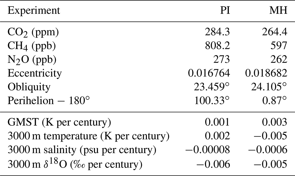
Table 1 Upper part: boundary conditions for pre-industrial and mid-Holocene experiments. Lower part: trends in global mean surface temperature (GMST) and mean oceanic temperature, salinity, and δ¹⁸O at 3000 m depth in the global ocean.

2.3 Data

To evaluate how well our model represents modern isotopic patterns, we compare our PI results with a compilation of isotopes in precipitation data and marine δ¹⁸O reanalysis data based on both model simulations and observations. Performing a pre-industrial simulation instead of a present-day one, which is a slightly warmer climate, probably adds a small negative bias in our modeled temperatures, and therefore in the modeled isotopic composition, compared to these data.

2.3.1 GNIP database

GNIP is a worldwide network for monitoring δ¹⁸O and δD in precipitation (IAEA, 2018), whose measurements were initiated in 1960 mainly by the International Atomic Energy Agency (IAEA) and the World Meteorological Organization (WMO). As in previous studies (Werner et al., 2016; Cauquoin et al., 2019), in our work only the records from stations in operation for at least 5 years within the period 1961 to 2007 are used. This subset of data is used to validate our modeled isotopic content of precipitation under PI conditions.

2.3.2 Ice core data

Like in Cauquoin et al. (2019), isotope measurements from a subset of 10 Antarctic (WAIS Divide Project Members, 2013) and 5 Greenland ice cores (Sundqvist et al., 2014) are selected and compared with our model results for the PI period. If data for the MH are available as well, we also compare the MH-minus-PI isotope composition between model simulations and ice core data. For each individual ice core record, we take the averaged δ¹⁸O value over the last 200 years and over the time interval of 6 ± 0.5 ka as a representative mean PI and MH value, respectively.

2.3.3 Speleothem calcite data

The Speleothem Isotope Synthesis and Analysis (SISAL) dataset provides a global compilation of speleothem δ¹⁸O records from 455 speleothems from 211 cave sites spanning the period from the Last Glacial Maximum (LGM) until the present (Comas-Bru et al., 2020). The δ¹⁸O in speleothem calcites (δ¹⁸O_c) is expressed with respect to the Pee Dee Belemnite (PDB) standard. Therefore the transformation equations described in Coplen et al. (1983) are applied to convert the speleothem δ¹⁸O value from the PDB to V-SMOW scale to enable a direct comparison between model results and speleothem records. Caution should be taken during model–data comparisons as the speleothem δ¹⁸O signals might be associated with seasonal climate conditions; for example speleothems from western Germany are more sensitive to the winter temperature and precipitation due to a strong influence of winter rainfall on the oxygen isotope composition of cave drip water (Wackerbarth et al., 2010). Following Comas-Bru et al. (2019), in the present study we select 30 speleothem sites (33 cores) for which isotopic values are available for both the MH (defined as the time interval of 6 ± 0.5 ka) and modern periods (1850–1990 CE).

2.3.4 Marine calcite data

Jonkers et al. (2020) have recently compiled a multiparameter marine data synthesis that contains time series spanning 0 to 130 ka. It is a data product focusing exclusively on time series with a robust chronology based on benthic foraminifera δ¹⁸O and radiocarbon dating. The dataset contains in total 896 time series of eight paleoclimate variables from 143 individual sites, among which 174 samples of planktonic foraminifera δ¹⁸O and 205 samples of benthic foraminifera δ¹⁸O are available. For both planktic and benthic foraminifera, a diversity of species have been measured. For more detailed information of this dataset, we refer to Jonkers et al. (2020).

To enable a direct comparison between model results and isotopic signals in the calcite shells of foraminifera, the equation described in Shackleton (1974) which links temperature during calcite formation (T) to the equilibrium fractionation of inorganic calcite precipitation around 16.9 ^∘C is used:

$$\begin{array}{}\text{(1)}& \begin{array}{rl}T& =\mathrm{16.9}-\mathrm{4.38}\times ({\mathit{\delta }}^{\mathrm{18}}{O}_{\mathrm{c}\left(\mathrm{PDB}\right)}-{\mathit{\delta }}^{\mathrm{18}}{O}_{\mathrm{oce}\left(\mathrm{PDB}\right)})\\ & +\mathrm{0.1}\times ({\mathit{\delta }}^{\mathrm{18}}{O}_{\mathrm{c}\left(\mathrm{PDB}\right)}-{\mathit{\delta }}^{\mathrm{18}}{O}_{\mathrm{oce}\left(\mathrm{PDB}\right)}{)}^{\mathrm{2}}.\end{array}\end{array}$$

In Eq. (1), δ¹⁸O_c(PDB) represents the isotopic composition of calcite on the Pee Dee Belemnite (PDB) scale, which can be converted to the SMOW scale via ${\mathit{\delta }}^{\mathrm{18}}{O}_{\mathrm{c}\left(\mathrm{SMOW}\right)}={\mathit{\delta }}^{\mathrm{18}}{O}_{\mathrm{c}\left(\mathrm{PDB}\right)}+\mathrm{0.27}$ (Hut, 1987).

2.3.5 Marine δ¹⁸O reanalysis data

A dynamically consistent database of global three-dimensional δ¹⁸O of seawater has been produced by Breitkreuz et al. (2018a). This set of data was generated based on an optimized simulation using an oceanic GCM constrained with climatological salinity and temperature data observed during 1951–1980 and global δ¹⁸O collected from 1950 to 2011. An adjoint method for variational data assimilation was used for optimization, enabling a consistency between the simulation and the observation. One thing to be noted is that the dataset shows a certain degree of bias in the surface levels in the Arctic Ocean which is caused by the rather low resolution applied in the model (2.8^∘ × 2.8^∘), as well as a lack of effect from isotopically highly depleted precipitation on the ocean in areas covered by sea ice. The final data were interpolated and provided with a regular 1^∘ × 1^∘ grid.

3 PI validation for water isotopes

The distribution of simulated precipitation-weighted annual mean δ¹⁸O in precipitation (hereafter referred to as δ¹⁸O_p) is depicted in Fig. 1a. The most notable characteristic is the decrease in δ¹⁸O_p with increasing latitude. This is due to the favorable correlation between surface temperature, condensation temperature, and the isotopic composition of meteoric water, particularly at high latitudes (Dansgaard, 1964). The so-called continental effect is also evident in Fig. 1a especially over Eurasia, where δ¹⁸O_p gets lighter toward the continental interior as the air masses moving inland experience multiple cycles of condensation and precipitation. Moreover, δ¹⁸O_p is typically lighter at higher altitudes such as the Himalayas and the Alps due to the so-called altitude effect.

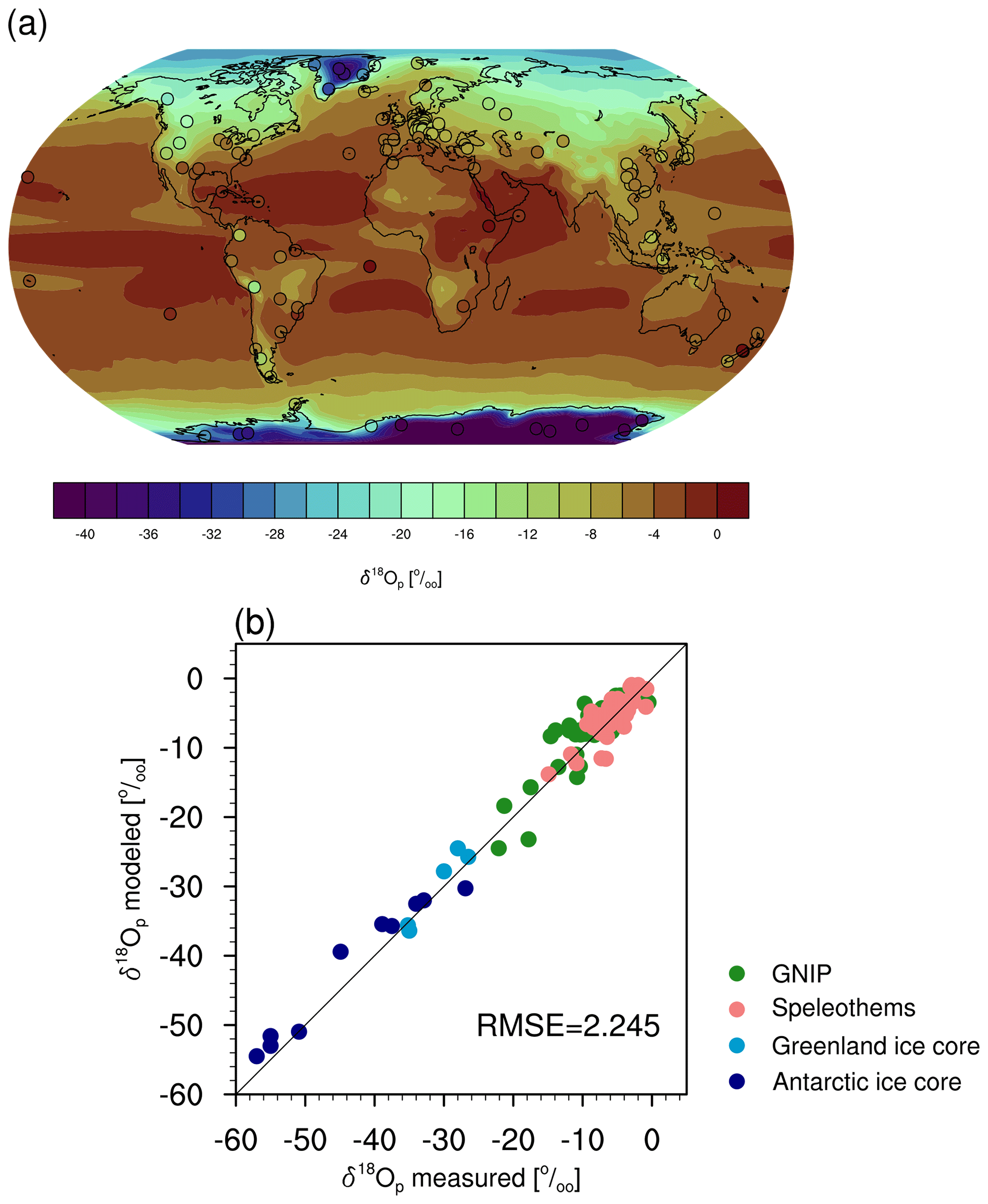
Figure 1 (a) Simulated pre-industrial (shading) and observed present-day (circles) precipitation-weighted annual mean δ¹⁸O in precipitation. (b) Scatter plot of modeled versus measured δ¹⁸O_p. Observation values are based on the GNIP database (IAEA, 2018), speleothems (Comas-Bru et al., 2020), and ice core records (WAIS Divide Project Members, 2013; Sundqvist et al., 2014).

To evaluate the performance of AWI-ESM-2.1-wiso in simulating the δ¹⁸O_p distribution under PI climate conditions, we compare measurements from the GNIP database, ice cores, and 33 selected speleothem records with simulated values at the same locations. Following the methodology described in the preceding section, we have used 70 values from the GNIP database which reflect the mean δ¹⁸O_p throughout the course of at least 5 calendar years. The results are shown in the circles of Fig. 1a and in the scatter plot of Fig. 1b, in which the reference 1:1 line represents a perfect model–data match. As illustrated in Fig. 1b, our model agrees well with the observed δ¹⁸O_p based on various archives with a root mean square error (RMSE) of 2.245 ‰. It is a big challenge for isotope-enabled models to reproduce correctly the isotope composition at sites with very low temperatures. A typical example is Antarctica, where earlier model simulations tend to overestimate the values of δ¹⁸O_p due to a possible warming bias. According to Masson-Delmotte et al. (2008), this underestimation can also be related to a low bias in water vapor for cold regions that favors higher δ¹⁸O_p values. Compared to earlier model studies (e.g., Werner et al., 2016; Cauquoin et al., 2019), AWI-ESM-2.1-wiso significantly reduces this model–data discrepancy over the Antarctic continent.

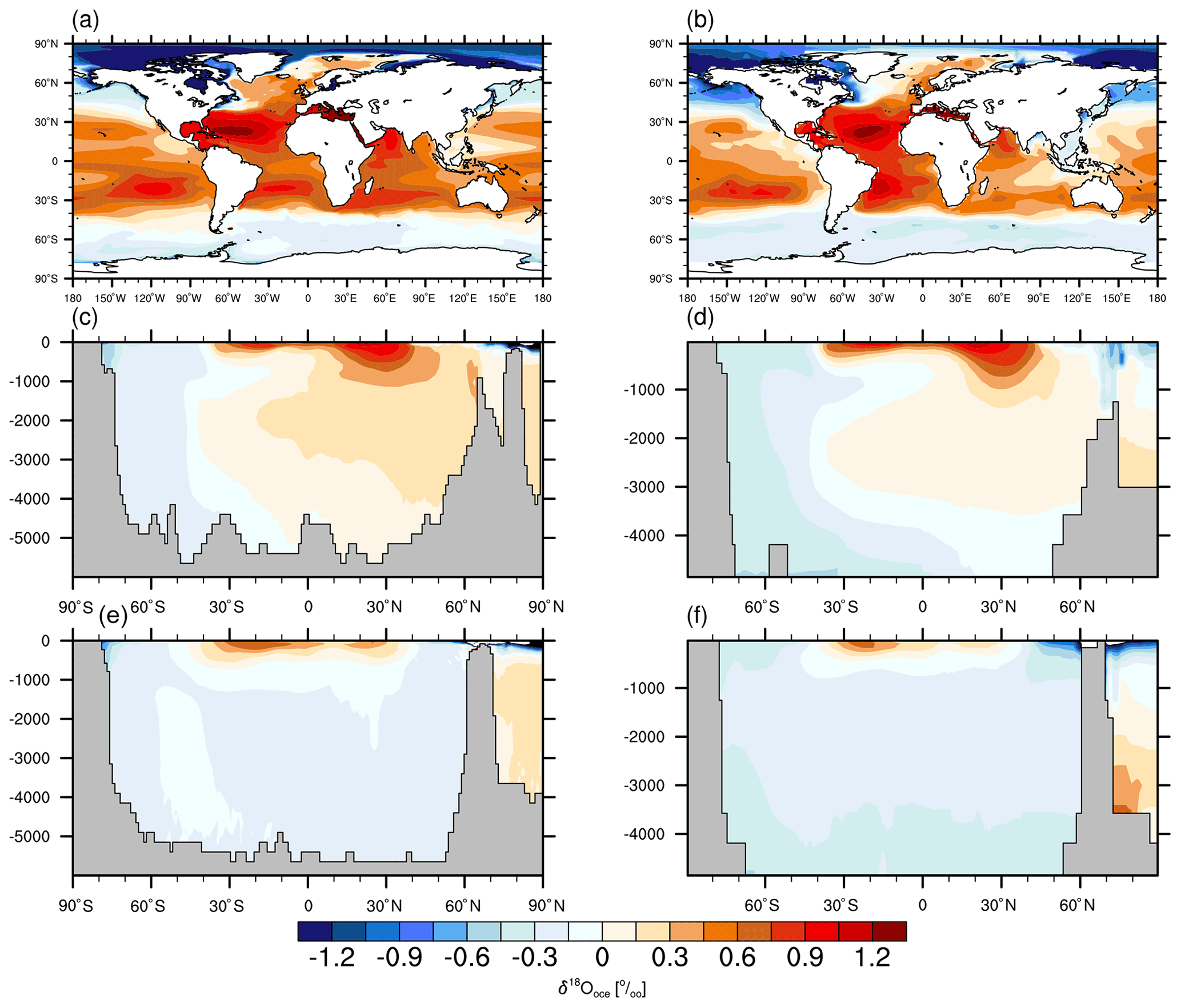
Figure 2 (a, b) Modeled (a) and assimilated (b) annual mean δ¹⁸O_oce in surface ocean from 0 to 10 m. (c, d) Modeled (c) and assimilated (d) zonal mean δ¹⁸O_oce across the Atlantic section. (e, f) As in (c, d) but for the Pacific section.

We compare our modeled annual mean δ¹⁸O_oce in sea surface water with the assimilation-based dataset of Breitkreuz et al. (2018a). As seen in Fig. 2a, the most enriched δ¹⁸O_oce as simulated by AWI-ESM-2.1-wiso can be found in the Mediterranean and Red Sea (more than 1.5 ‰) and secondly in the North Atlantic Ocean with δ¹⁸O_oce values reaching 1.2 ‰ due to intense evaporation and net freshwater export. In general, δ¹⁸O_oce decreases from middle to high latitudes as a consequence of the latitudinal temperature gradient. Since the subtropics experience more evaporation than the tropics, the isotopic composition of the subtropical surface waters is higher than that of the equatorial regions. Furthermore, the most depleted δ¹⁸O_oce can be found in the Arctic Ocean, Baffin Bay, and, to a lesser degree, the Pacific Ocean north of 40^∘ N. Similar patterns can be seen in the marine δ¹⁸O reanalysis data (Fig. 2b).

Despite the model–data agreement on the aforementioned significant aspects in the spatial structures of sea surface δ¹⁸O_oce, there are a number of discrepancies identified between model and data in terms of the δ¹⁸O_oce magnitudes. For instance, our model underestimates the isotopic composition of the South Atlantic and overestimates the δ¹⁸O values in the Southern Ocean. Mismatches between our model simulation and marine δ¹⁸O reanalysis data may result from model bias in representing freshwater export or net precipitation. Moreover, a warming bias across the Southern Ocean simulated by AWI-ESM-2.1-wiso can lead to increased evaporation that favors larger δ¹⁸O_oce values.

For further evaluation, the simulated and assimilated zonal means of δ¹⁸O_oce at depths for both the Atlantic and Pacific sectors are shown in Fig. 2c–f. In the Atlantic, the most enriched δ¹⁸O_oce values are found near the ocean's surface and subsurface due to the considerable influence of air–sea interactions. The North Atlantic Deep Water (NADW) is isotopically enriched, although with a smaller magnitude in δ¹⁸O_oce than the upper layers. Deep water convection in the Atlantic Ocean is responsible for the enrichment in NADW δ¹⁸O_oce. Both the Antarctic Intermediate Water (AAIW) and Antarctic Bottom Water (AABW) are depleted as they are supplied by Southern Ocean surface water, which has negative δ¹⁸O_oce values. The distributions of δ¹⁸O_oce in the subsurface and deep waters of the Pacific are distinctly different from those of the Atlantic. Since the deep water formation of the Pacific is substantially weaker than the Atlantic, the enriched seawater is confined to depths of 0–1000 m in the tropics and subtropics. Pacific intermediate and bottom depths are primarily dominated by negative δ¹⁸O_oce.

Our simulated zonal mean δ¹⁸O_oce are in good agreement with Breitkreuz et al. (2018a) for both the Atlantic and Pacific basins. However, in certain regions, our simulation deviates from the data in the magnitudes of δ¹⁸O_oce. An example is the Southern Ocean, where our model exhibits enrichment biases across the whole water column. Moreover, AWI-ESM-2.1-wiso tends to overestimate the δ¹⁸O_oce values of Antarctic and Pacific bottom water.

These comparisons demonstrate that AWI-ESM-2.1-wiso is capable of capturing the present-day spatial distribution of δ¹⁸O in precipitation and seawater, as indicated by the consistency between model results and available datasets. It strengthens our confidence in the quality of the MH simulation examined in the subsequent sections.

4 Climate and isotope differences between MH and PI

4.1 Differences in climate signals

Stable water isotopes are closely linked to changes in standard climate variables, among which the most important ones are the surface air temperature (SAT), precipitation, and evaporation. Therefore before examining the isotope anomalies between the MH and PI periods, we firstly examine the simulated climate differences.

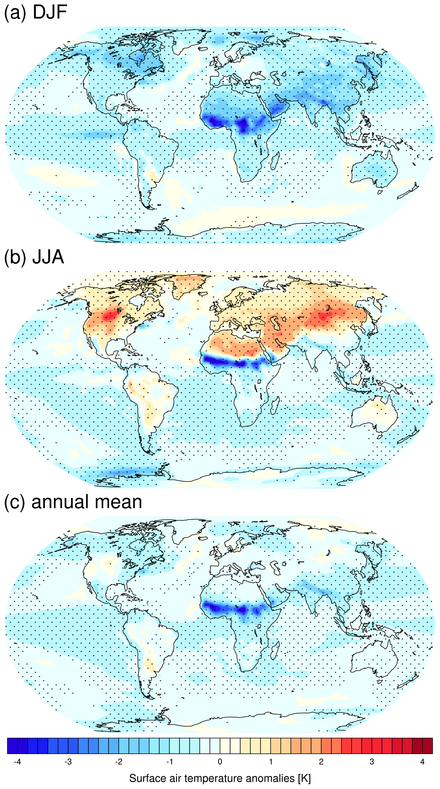
Figure 3 Simulated anomalies (MH–PI) of surface air temperature for (a) DJF, (b) JJA, and (c) annual mean. The marked area has a significance level greater than 95 % based on Student's t test. Units: kelvin (K).

Figure 3 depicts the simulated anomalies in seasonal and annual mean SAT, which imply an enhanced seasonality in the Northern Hemisphere, i.e., a cooling of boreal winter and a warming of boreal summer, consistent with results from model ensemble means (Brierley et al., 2020). Such seasonality enhancement is caused by changes in the orbital parameters which lead to the redistribution of latitudinal and seasonal incoming solar insolation at the top of the atmosphere. Specifically, more insolation is received in June–August (JJA) than in December–February (DJF) during the MH relative to the PI period. Another prominent aspect is the year-round cooling of the Sahara, in conjunction with a northward migration of the tropical rain belt, as well as increased precipitation and cloudiness over the Sahara. Such cooling coincides with other climate models (Brierley et al., 2020) but contradicts proxy records which document a general warming over that region (Bartlein et al., 2011). The warming registered in the pollen-based proxy, however, mainly reflects an earlier growth season during the MH (Bartlein et al., 2011). During DJF, Antarctica presents a moderate cooling, while in JJA it is characterized by non-uniform changes with a warming in the east and cooling in the west.

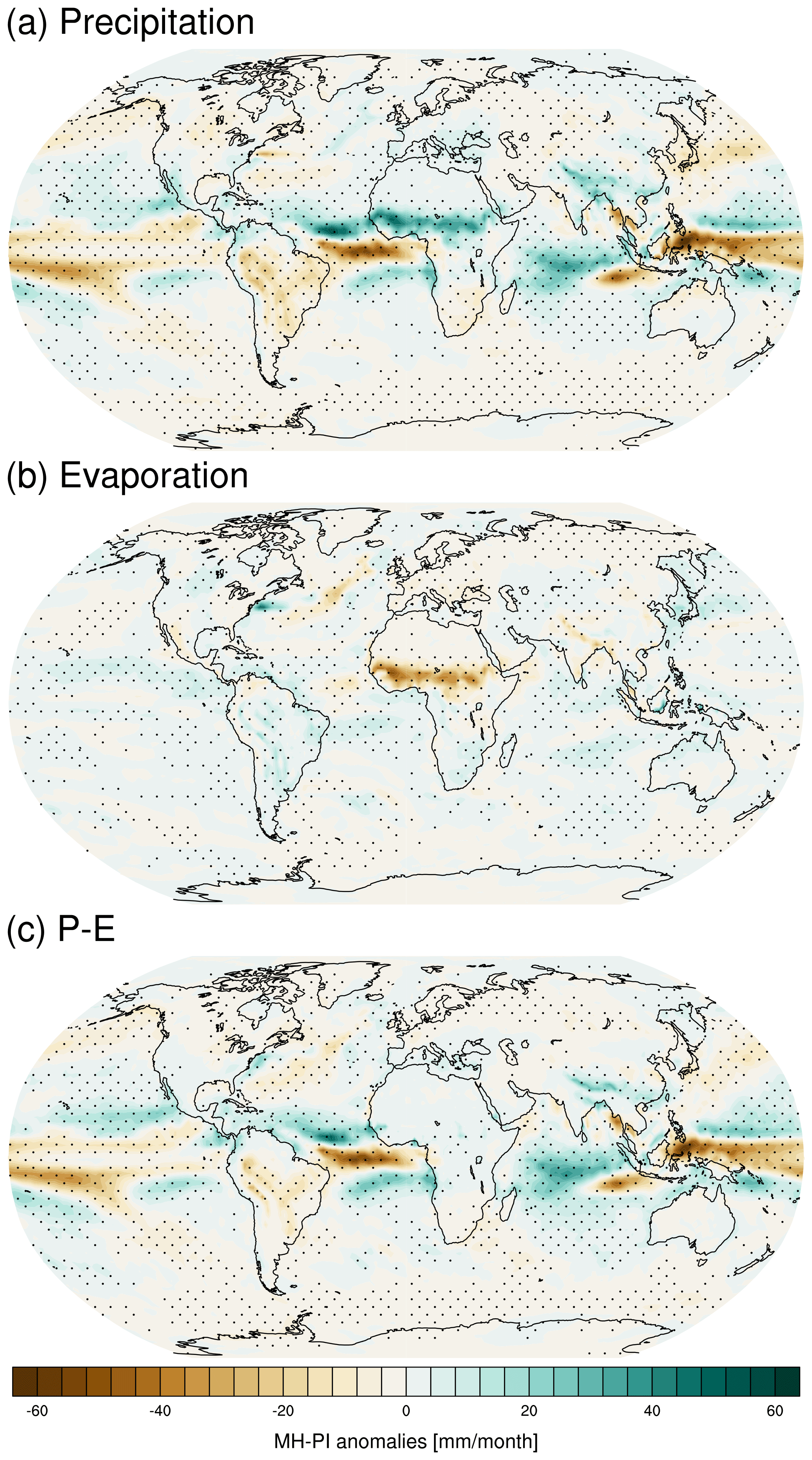
Figure 4 Simulated anomalies (MH–PI) of annual mean (a) precipitation, (b) evaporation (positive downward), and (c) precipitation minus evaporation. The marked area has a significance level greater than 95 % based on Student's t test. Units: millimeters per month.

Simulated changes in annual mean precipitation between the MH and PI periods are shown in Fig. 4a. The most striking pattern is the enhanced precipitation over the North African monsoon region, which is associated with a northward displacement of the Intertropical Convergence Zone (ITCZ). There is also an increase in precipitation, albeit to a lesser extent, in other Northern Hemisphere monsoon regions such as North America and South Asia. The tropical Pacific experiences a substantial drying in the MH compared to the PI period, while the Indian Ocean experiences wetter conditions. In general, our results regarding the MH-minus-PI precipitation agree well with other climate models (Brierley et al., 2020) as well as pollen-based reconstructions (Bartlein et al., 2011). The evaporation anomalies over the globe are relatively small, except for North Africa where large anomalous evaporation occurs (Fig. 4b). The distribution of changes in net precipitation, defined as precipitation minus evaporation (P−E), as shown in Fig. 4c, resembles that of the precipitation changes, with an exception over North Africa where no clear change in P−E is detected due to a compensation between the enhancement of both precipitation and evaporation.

4.2 Differences in isotopic signals

In this section we turn to analyze the anomalous isotope composition between the MH and PI periods. The shadings in Fig. 5a represent the simulated changes in the precipitation-weighted annual mean δ¹⁸O_p. Although only modest annual mean warming (less than 0.2 K) is found over Greenland and the Arctic, this nevertheless leaves a noticeable imprint on the isotope composition of precipitation, with δ¹⁸O_p enriched by up to 1 ‰ in the MH with respect to the PI period. Such a change may mainly reflect the regional warming during summer. Another clear picture in Fig. 5a is the depletion of δ¹⁸O_p over North Africa (more than −4 ‰) and South Asia (up to −2 ‰), closely correlated with increased monsoonal rainfall and reduced surface air temperature. The Antarctic continent is generally dominated by enriched δ¹⁸O_p except for localized regions that are slightly depleted. Over the remaining land surfaces, AWI-ESM-2.1-wiso simulates small to moderate negative MH–PI anomalies down to −1 ‰. Concerning the ocean region, our model presents more positive δ¹⁸O_p values over the Indo-Pacific warm pool as a consequence of reduced precipitation during the MH. In addition, large positive δ¹⁸O_p anomalies in the Amundsen Sea are produced by our model because of a pronounced JJA warming in the MH relative to the PI period.

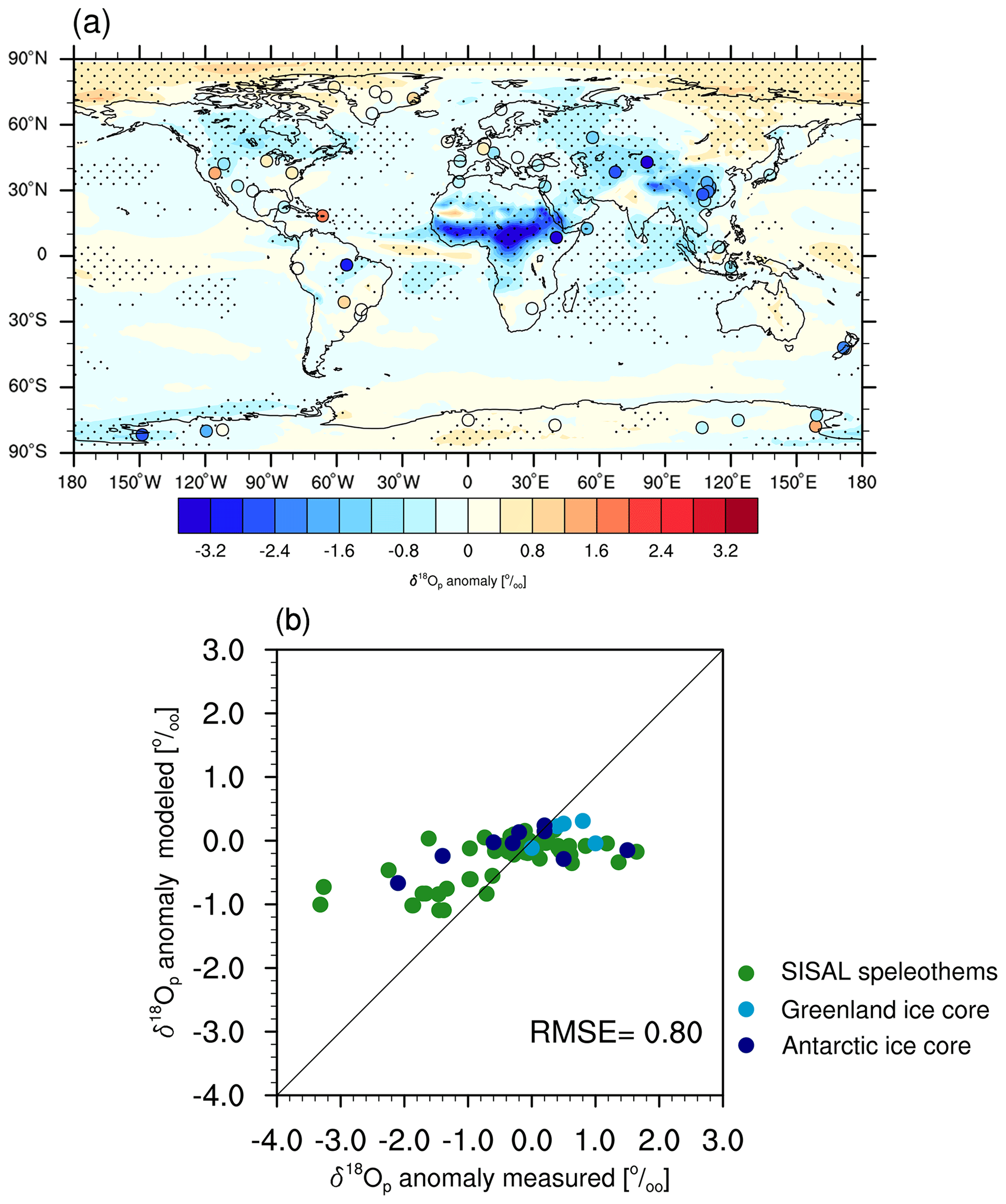
Figure 5 (a) Simulated (shading) and reconstructed (circles) anomalies in precipitation-weighted annual mean δ¹⁸O in precipitation between the MH and PI periods. The marked area has a significance level greater than 95 % based on Student's t test. (b) Scatter plot of modeled versus reconstructed δ¹⁸O_p anomalies. Units: permil (‰).

We assess our simulated MH-minus-PI δ¹⁸O_p against ice core and speleothem calcite data, which are shown in Fig. 5a (circles) and b. Our model results generally agree with the proxy records for the δ¹⁸O_p changes over Greenland, Europe, and part of North America. However, while AWI-ESM-2.1-wiso simulates a moderate change in δ¹⁸O_p across the globe (i.e., −1.3 ‰ to +0.4 ‰), the speleothem data reveal a wide range of δ¹⁸O_p changes, being from −3.4 ‰ to +2 ‰ (Fig. 5b). Spatially, such bias can be detected over South Asia, tropical Africa, South America, and western Antarctica, where our model severely underestimates the change in δ¹⁸O_p.

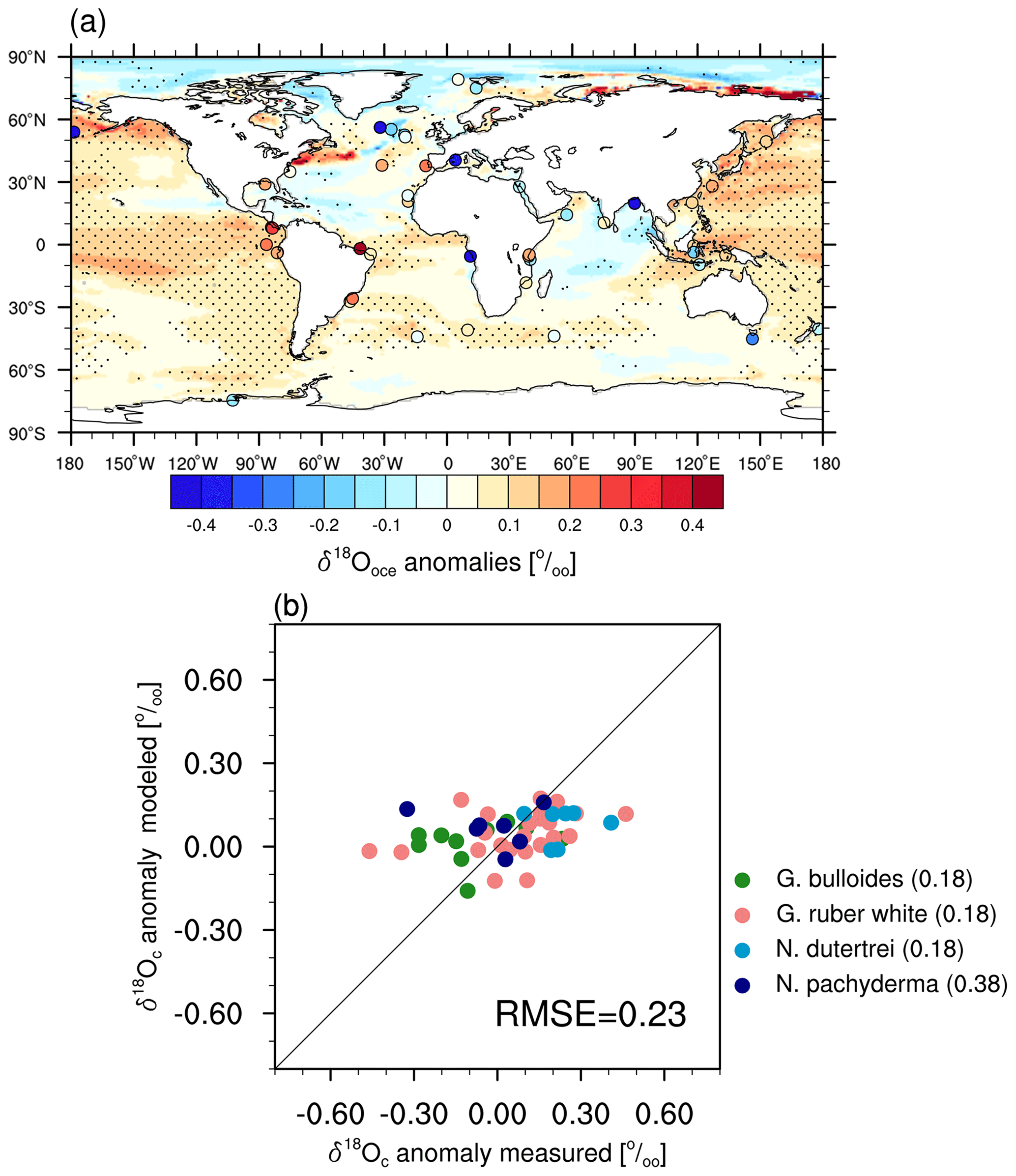
Figure 6 (a) Simulated (shading) and reconstructed (circles) anomalies in annual mean δ¹⁸O_c in ocean surface waters between the MH and PI periods. The marked area has a significance level greater than 95 % based on Student's t test. (b) Scatter plot of modeled versus reconstructed δ¹⁸O_c anomalies. The numbers in the legend display the RMSE values for each planktonic foraminifera type. Units: permil (‰).

Figure 6a shows the simulated changes in annual mean δ¹⁸O_c in ocean surface water between the MH and PI periods versus available reconstruction data based on planktonic foraminifera (Jonkers et al., 2020). We only choose species which cover more than six locations on a global scale. Here δ¹⁸O_c refers to δ¹⁸O in calcite, calculated from the simulated δ¹⁸O in seawater and ocean temperature upon Shackleton (1974). This conversion is required to enable a direct comparison between model results and isotopic signals in the calcite shells of planktonic foraminifera (see Methodology section). It is apparent in Fig. 6a that in our model the Pacific Ocean, South Atlantic, and Southern Ocean are more δ¹⁸O_c-enriched during the MH compared to the PI period, generally in line with the proxy records with the exception of a few proxy reconstructions exhibiting a depletion signal. A depletion in the δ¹⁸O_c across the Indian Ocean is simulated in our model as a result of an increase in net precipitation. The scatter plot of Fig. 6b indicates that our simulated annual mean δ¹⁸O_c anomalies fall within a narrower range (−0.2 ‰ to 0.2 ‰) compared to the reconstructed anomalies (ranging from −0.5 ‰ to 0.5 ‰). The calculated RMSE between modeled and measured MH–PI δ¹⁸O_c changes is 0.18 ‰ for the species of Globigerina bulloides, Globigerinoides ruber albus, and Neogloboquadrina dutertrei. The modeled δ¹⁸O_c anomalies are mostly close to the Neogloboquadrina pachyderma-based measurements; nonetheless, our model result deviates largely from the observation for one Neogloboquadrina pachyderma location documenting a significant depletion in δ¹⁸O_c, leading to a RMSE of 0.38 ‰ for this planktonic foraminifera species. The RMSE across all the species mentioned above is 0.23 ‰.

5 Climate–isotope relationship in MH and PI periods

A strong positive correlation between the annual mean surface temperature and the precipitation-weighted δ¹⁸O_p was firstly recognized by Dansgaard (1964). This relationship has served as the foundation for a lot of paleoclimate research in which the temporal evolution of past temperature for a certain region is derived from isotopic proxies. Therefore, it is essential to examine the following. (1) Is the modeled spatial and temporal isotope–temperature relationship under PI and MH conditions identical to the observed modern spatial gradient in various regions? (2) Under which condition can we support the application of a modern spatial isotope–temperature gradient in reconstructing past climate changes? To answer these questions, in the following we perform further analysis on the spatial and temporal relationship between δ¹⁸O_p and temperature based on both PI and MH simulations. In addition, the temporal relationships between isotope and precipitation are investigated as well.

5.1 Spatial δ¹⁸O_p–temperature gradient

To determine the simulated global spatial δ¹⁸O_p–temperature slope, we use the δ¹⁸O_p and surface air temperature modeled at all grid cells with an annual mean temperature below 20 ^∘C. This criterion is taken to restrict our analysis to regions with a dominant temperature dependency. Our modeled global spatial δ¹⁸O_p–temperature slope has a value of 0.71 ± 0.005 ‰ ^∘C⁻¹ for the PI period (Fig. 7a; here the uncertainty is calculated from the interannual standard deviation), similar to the value of 0.69 ‰ ^∘C⁻¹ derived from observations (Dansgaard, 1964). Compared to former studies using isotope-enabled climate models (Cauquoin et al., 2019; Risi et al., 2010; Gierz et al., 2017), our result is more in line with observations. The same as for the PI experiment, our MH experiment also yields a global spatial δ¹⁸O_p–temperature slope of 0.71 ± 0.005 ‰ ^∘C⁻¹ (Fig. 7f). To compute the isotope–temperature slope of polar regions, we take only grid boxes around the ice core locations. Over Greenland, our modeled δ¹⁸O_p–temperature gradients under present-day and MH conditions are 0.76 ± 0.042 and 0.74 ± 0.045 ‰ ^∘C⁻¹, respectively (Fig. 7b, g), higher than the value obtained from modern observations (0.67 ‰ ^∘C⁻¹) (Johnsen et al., 1989) and previous model studies using MPI-ESM-wiso (0.71 ‰ ^∘C⁻¹) (Cauquoin et al., 2019) and ECHAM4 (0.58 ‰ ^∘C⁻¹) (Werner et al., 2000). However, a much smaller Holocene spatial isotope–temperature slope, ranging from 0.43 ‰ ^∘C⁻¹ to 0.53 ‰ ^∘C⁻¹, was estimated based on ice core records and borehole temperatures for the Greenland ice sheet (Vinther et al., 2009).

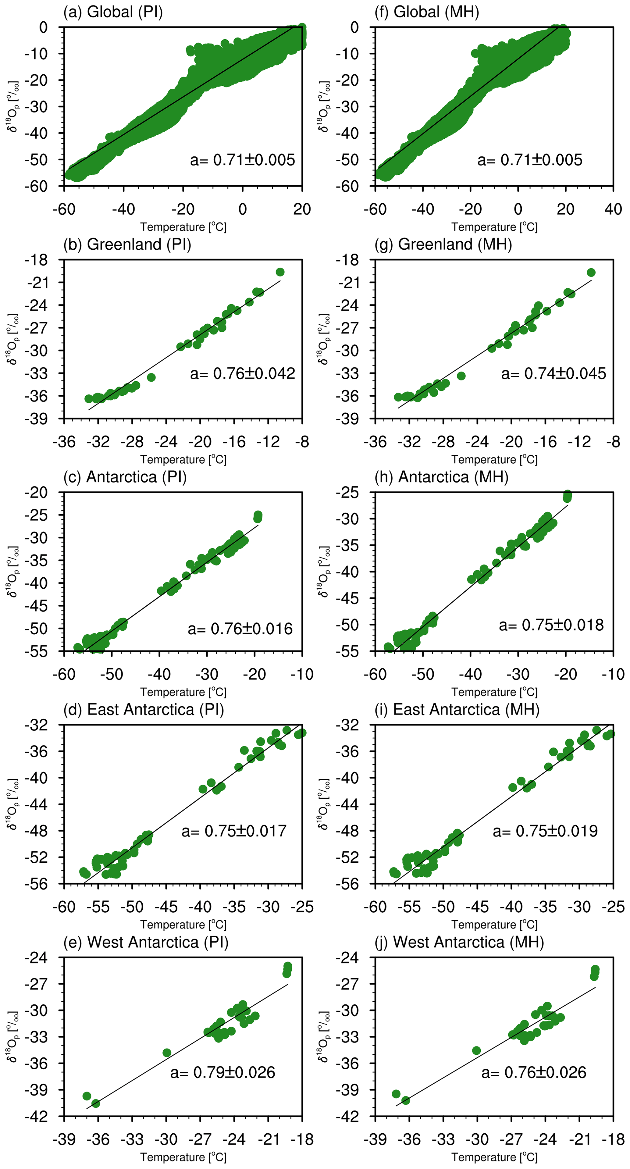
Figure 7 Simulated PI spatial δ¹⁸O_p–temperature gradient for (a) all global grid boxes with an annual mean temperature below 20 ^∘C, (b) Greenland, (c) Antarctica, (d) East Antarctica, and (e) West Antarctica. (f)–(j) Same as in (a)–(e) but for the MH.

For Antarctica, our model generates a spatial isotope–temperature slope of 0.76 ± 0.016 ‰ ^∘C⁻¹ for the PI period and 0.75 ± 0.018 ‰ ^∘C⁻¹ for the MH (Fig. 7c), slightly lower than the mean observed value of 0.8 ‰ ^∘C⁻¹ (Masson-Delmotte et al., 2008). For East Antarctica under both present-day and mid-Holocene conditions, our simulated spatial δ¹⁸O_p–temperature gradient is around 0.75 ‰ ^∘C⁻¹. In the PI experiment, the gradient for West Antarctica is a little bit larger (0.79 ± 0.026 ‰ ^∘C⁻¹) than for the East Antarctic. But for the MH we find no clear distinction of the spatial isotope–temperature relationship between West and East Antarctica. Our simulation results suggest a similar δ¹⁸O_p–temperature relationship between the MH and PI periods, both globally and regionally. This also indicates that the moderate changes in δ¹⁸O_p and δ¹⁸O_oce, simulated in our model, are more likely related to weak responses of the climate to MH boundary conditions. In addition, the spatial δ¹⁸O_p–temperature relationship can be affected by the criteria of data selection, e.g., if coastal areas or only higher-altitude sites on the ice sheet are included (Sjolte et al., 2011).

It is important to note that there is a significant regional dependency found for the spatial isotope–temperature slope (Sjolte et al., 2011) and that the spatial slope might differ from the temporal slope due to changes in the seasonality of precipitation (e.g., Werner et al., 2000), moisture source regions (e.g., Delaygue et al., 2000b), or polar amplification feature (Guan et al., 2016). In the following section, we aim to analyze the temporal relationship between our simulated δ¹⁸O_p and climate variables.

5.2 Temporal relationship

Here we examine the simulated MH-to-PI temporal relationship between δ¹⁸O_p and surface air temperature changes, defined as

$$\begin{array}{}\text{(2)}& m=({\mathit{\delta }}^{\mathrm{18}}{O}_{\mathrm{p},\mathrm{MH}}-{\mathit{\delta }}^{\mathrm{18}}{O}_{\mathrm{p},\mathrm{PI}})/(T_{\mathrm{MH}}-T_{\mathrm{PI}}).\end{array}$$

In accordance with previous studies (Cauquoin et al., 2019; Gierz et al., 2017), we only consider grid points with a mean temperature below 20 ^∘C for both the MH and PI periods, thereby excluding from our analysis tropical regions where local variances of δ¹⁸O_p are strongly controlled by changes in precipitation amount and moisture source region. To avoid numerical errors in calculated temporal relationships caused by very small MH–PI temperature changes, another criterion is adopted, which is that the absolute change in T between the two time intervals (i.e., T_MH−T_PI) must be non-negligible, namely not less than 0.5 ^∘C. Applying such a threshold can also ensure a temperature dependency of the isotope changes. Several approaches are available for T in Eq. (1). As a first step we define T as the mean annual temperature (MAT) and show in Fig. 8a the modeled MH-to-PI temporal gradient between δ¹⁸O_p and MAT changes. Over southeastern China, the gradients approach 0.9 ‰ ^∘C⁻¹, significantly greater than the observed global modern spatial gradient of 0.69 ‰ ^∘C⁻¹ (Dansgaard, 1964). This high value obtained from our model is attributable to the combined impacts of an increase in monsoonal rainfall (Fig. 4a) and a decrease in surface air temperature (Fig. 3). Greenland and the majority of Antarctica, where the polar ice core samples are collected, are dominated by missing data as the MAT changes there are not substantial (Fig. 3).

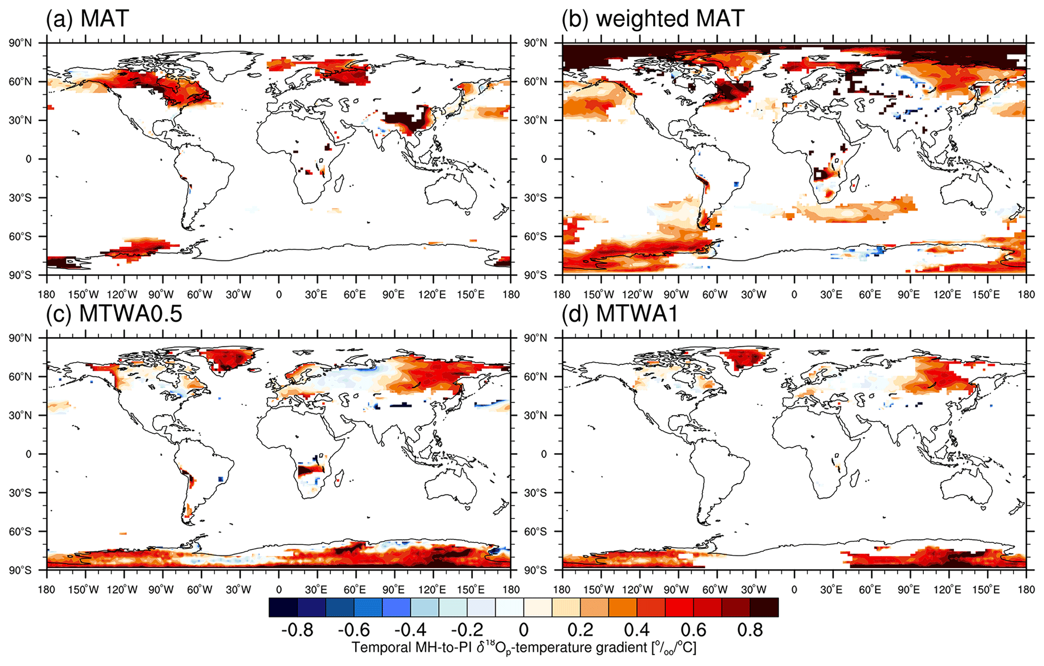
Figure 8 (a) Simulated temporal MH-to-PI δ¹⁸O_p–temperature gradient for all grid boxes with mean annual temperature (MAT) for both PI and MH periods being lower than 20 ^∘C and the absolute change in temperature between the MH and PI periods being at least 0.5 ^∘C. (b) Same as in (a) but using the precipitation-weighted annual mean temperature. (c) Same as in (a) but using the temperature of the warmest month (MTWA). (d) Same as in (c) but with the absolute change in MTWA being at least 1 ^∘C. Units: permil per degree Celsius (‰ ^∘C⁻¹).

In the part that follows, T is defined as the simulated mean temperature of the warmest month (MTWA), i.e., the mean temperature of July and January for the Northern Hemisphere and Southern Hemisphere, respectively, and the calculated global distribution of temporal gradients is given in Fig. 8c. As can be seen, δ¹⁸O_p–MTWA temporal gradients are present across middle and high latitudes of the Northern Hemisphere, with the bulk of values varying from 0.2 ‰ ^∘C⁻¹ to 0.8 ‰ ^∘C⁻¹. Over Greenland, the mean temporal gradient averaged over ice core sites is 0.64 ‰ ^∘C⁻¹, close to the observed modern spatial value of 0.67 ‰ ^∘C⁻¹. East and West Antarctica, respectively, presents a mean coefficient of 0.55 ‰ ^∘C⁻¹ and 0.39 ‰ ^∘C⁻¹. However, certain locations of Antarctica are found to have negative δ¹⁸O_p–MTWA temporal gradients. This reflects either a “selection” or a “recorder” problem (Gierz et al., 2017). The former may arise when temperature is not the primary factor affecting the isotope signal, implying that the δ¹⁸O_p changes are strongly influenced by other processes such as the precipitation amount, moisture origin, and water transport pathways. In this instance, a stricter threshold for the temperature change might be beneficial. The recorder problem is associated with pronounced changes in seasonality or intermittency of the precipitation rate (Sime et al., 2009). This problem can be reduced by the use of precipitation-weighted mean annual temperature instead of arithmetic MAT.

To decrease the selection problem, we increase the threshold for MH-minus-PI temperature to 1 ^∘C, and the resulting global map of temporal δ¹⁸O_p–MTWA gradients is presented in Fig. 8d. Applying this constraint on MTWA removes the most negative gradients from the Antarctic continent. The mean temporal gradient becomes 0.60 ‰ ^∘C⁻¹ for both Greenland and Antarctic ice core locations. Our results suggest that the spatial δ¹⁸O_p–T slope observed under the modern climate could be a surrogate for the MH-to-PI temporal isotope–temperature gradient during the warmest month/season over Greenland and Antarctica.

In addition, to address the recorder problem, we recalculated the temporal δ¹⁸O_p–T gradients, with T being the precipitation-weighted mean annual temperature, in the same way as in Gierz et al. (2017) and Cauquoin et al. (2019). We obtain a mean temporal δ¹⁸O_p–T gradient of 0.36 ‰ ^∘C⁻¹ for Greenland and 0.22 ‰ ^∘C⁻¹ for Antarctica, much lower than the observed spatial slopes in the present day (Table 2). As is apparent in Fig. 8b, there are still a number of grid cells with a negative gradient, indicating that the change in seasonality or intermittency of the precipitation is not the primary reason for the negative gradient values.

Instead of using an arbitrary threshold, we propose an alternative method to calculate the temporal gradient of δ¹⁸O_p–temperature based on the significance of temperature anomalies. In Fig. S2a, we only consider regions with significant changes in MAT (sig. MAT). Positive gradients are observed in parts of Northern Hemisphere continents; however, data are missing for Greenland due to the minor change in annual mean temperature between the MH and PI periods, which is statistically insignificant. The simulated temporal isotope–temperature gradient is about 0.6 ‰ ^∘C⁻¹ for Antarctica. Especially, the gradient value of 0.61 ‰ ^∘C⁻¹ for West Antarctica is closer to observations compared to other T definitions. For regions with significant changes in MTWA (sig. MTWA), we obtain a gradient pattern similar to that of MTWA0.5 (cf. Figs. S2 and 8c, and refer to Table 2 for detailed values). Additionally, we calculate the isotope–temperature gradient for the monsoon seasons (sig. T-monsoon), specifically June–September (JJAS) for the Northern Hemisphere and December–March (DJFM) for the Southern Hemisphere. As depicted in Fig. S2c, unrealistic high values are observed in the Arctic Ocean, while unrealistic negative values are obtained for North America, the Bering Sea, and midlatitude Asia. The MH-to-PI temporal isotope–temperature gradient for Greenland ice core locations is estimated to be 0.61 ‰ ^∘C⁻¹. However, the δ¹⁸O_p–temperature temporal gradient for Antarctica is largely underestimated (Table 2). Applying a threshold of 0.5 ^∘C for temperature changes (sig. T-monsoon0.5) improves the gradient values for Antarctica, but they still remain considerably smaller than the observations (Fig. S2d, Table 2). Further increasing the temperature threshold to 1 ^∘C (sig. T-monsoon1) excludes most areas from our calculation (Fig. S2e).

Table 2 Mean temporal MH-to-PI δ¹⁸O_p–T gradient averaged over the ice core locations for different T definitions, as well as the observed spatial δ¹⁸O_p–T gradient in the present day. Units: permil per degree Celsius (‰ ^∘C⁻¹).

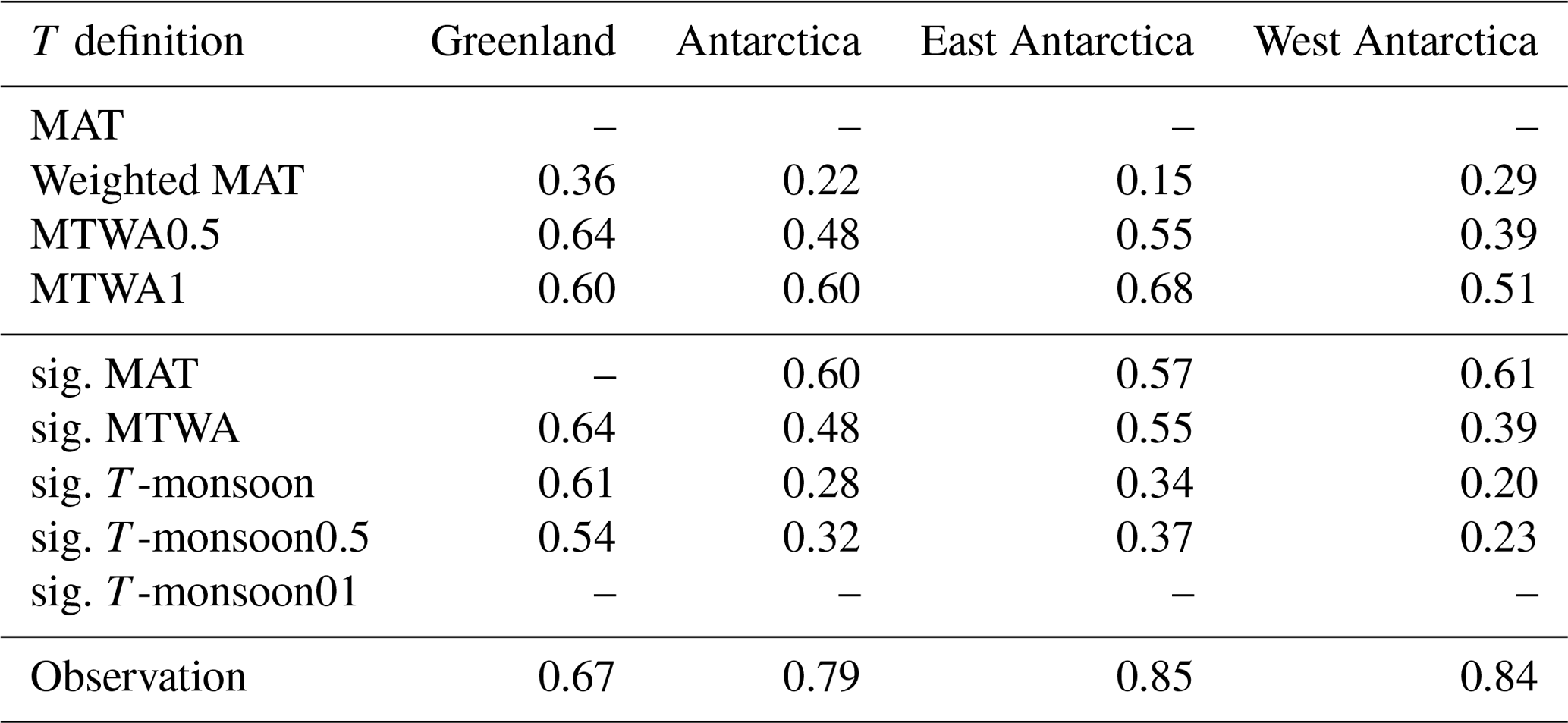
Table 3 Simulated mean anomaly of T across ice core locations for different T definitions, as well as the reconstructed T anomaly based on ice core records and observed present-day spatial δ¹⁸O_p–T slopes. Units: degree Celsius (^∘C).

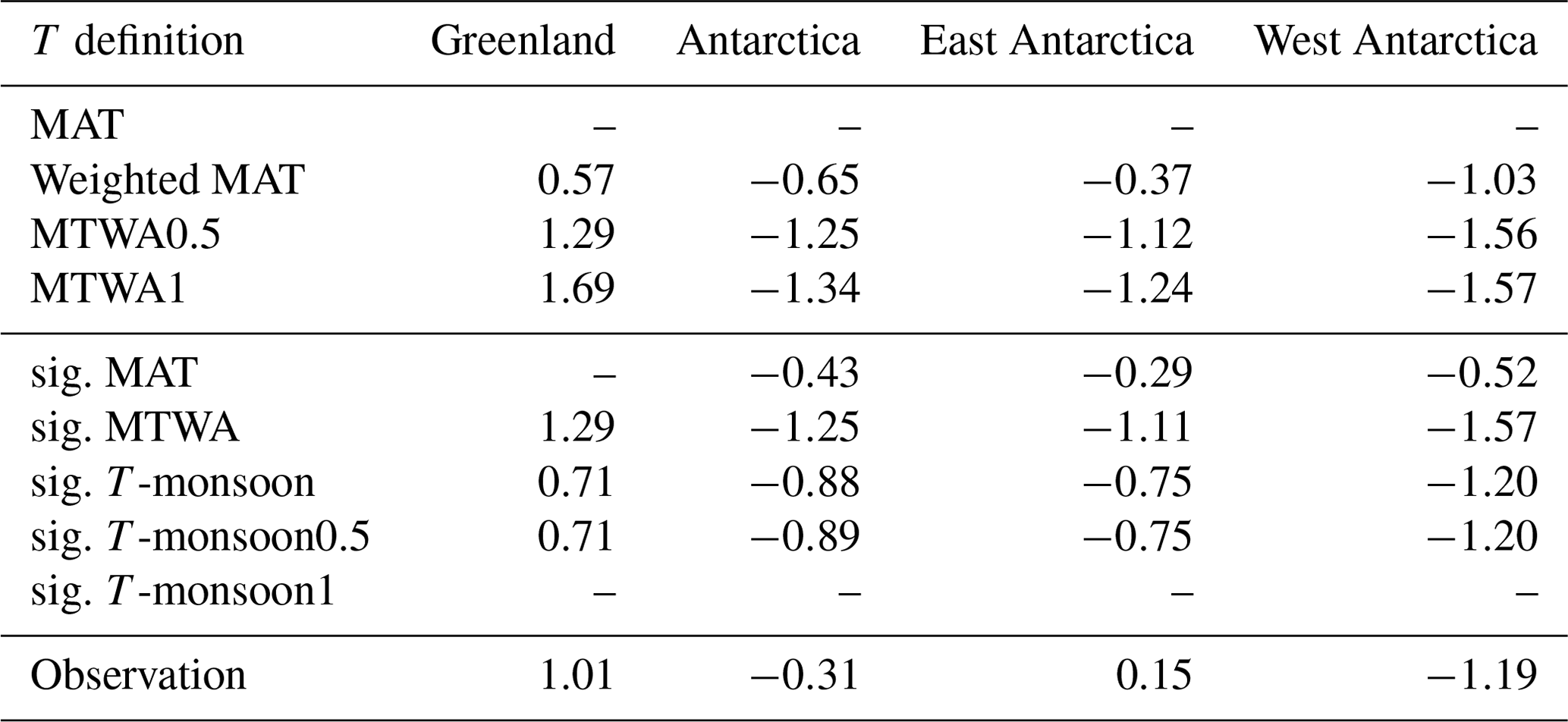
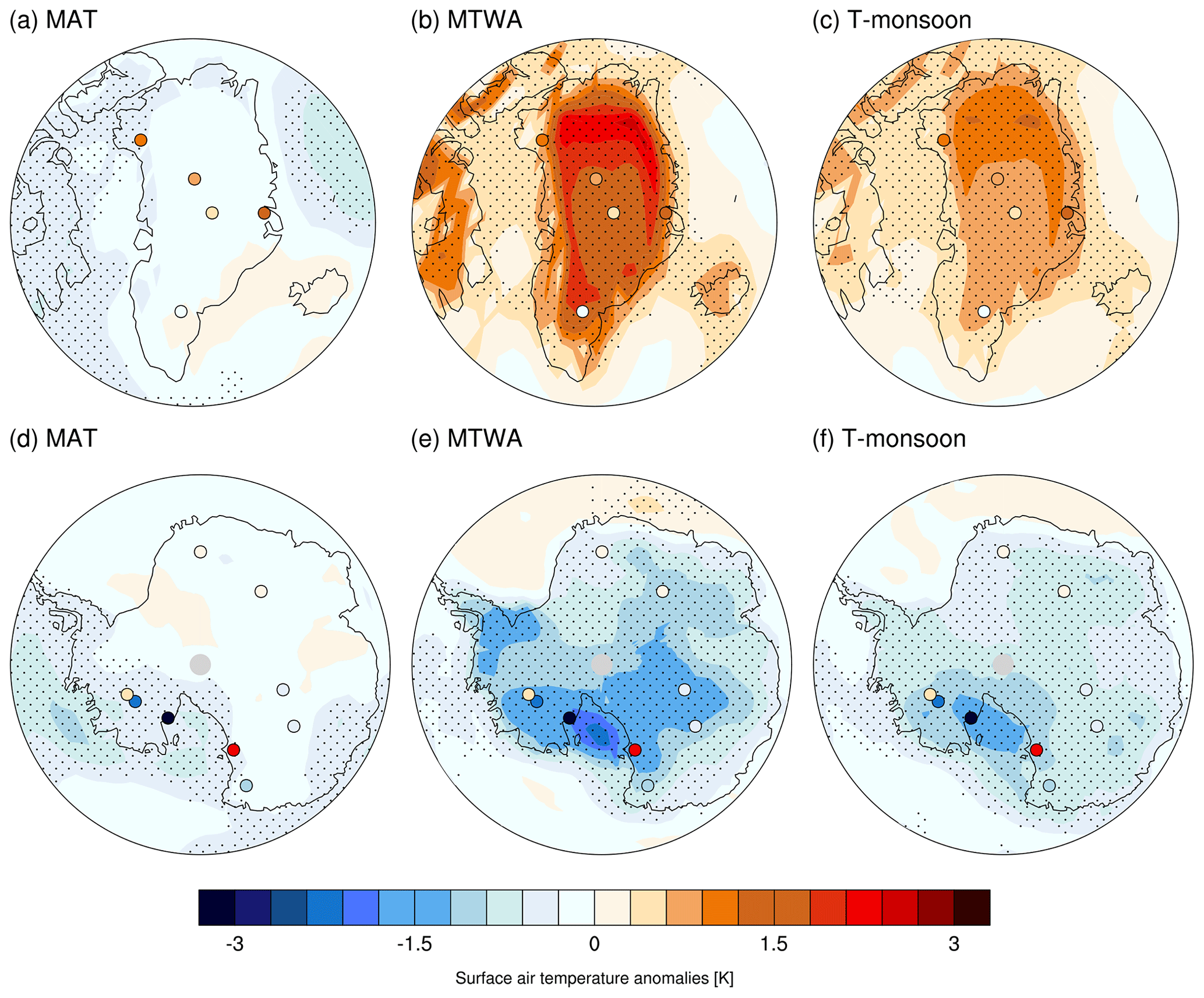
Figure 9 Simulated MH–PI T anomalies for (a–c) Greenland and (d–f) Antarctica, with T being (a, d) MAT, (b, e) MTWA, and (c, f) T-monsoon. The marked area has a significance level greater than 95 % based on Student's t test. Circles represent reconstructed temperature anomalies based on ice core records. Units: degree Celsius (^∘C).

For each defined temperature (T), we calculate the average temperature anomalies (MH-minus-PI T anomalies) and compare the results with temperature reconstructions based on ice core δ¹⁸O_p values and observed modern spatial δ¹⁸O_p–temperature slopes. As shown in Fig. 9a, there is a lack of consensus between the simulated MAT anomalies and the values obtained from proxy records in Greenland. However, it is evident that the MTWA and T-monsoon exhibit a relatively stronger agreement with the observed data (Fig. 9b, c). Table 3 indicates that the proxy-based mean temperature anomaly over Greenland is 1.01 ^∘C. Notably, the MTWA0.5 and sig. MTWA definitions provide a mean temperature anomaly of 1.29 ^∘C across the Greenland ice core locations, which is relatively closer to the observed data compared to other T definitions. In Antarctica, non-uniform temperature anomalies are observed, with modest changes in some areas and more significant cooling and warming in other regions. However, our model shows a general cooling trend across the entire Antarctic continent for all T definitions (Fig. 9d–f).

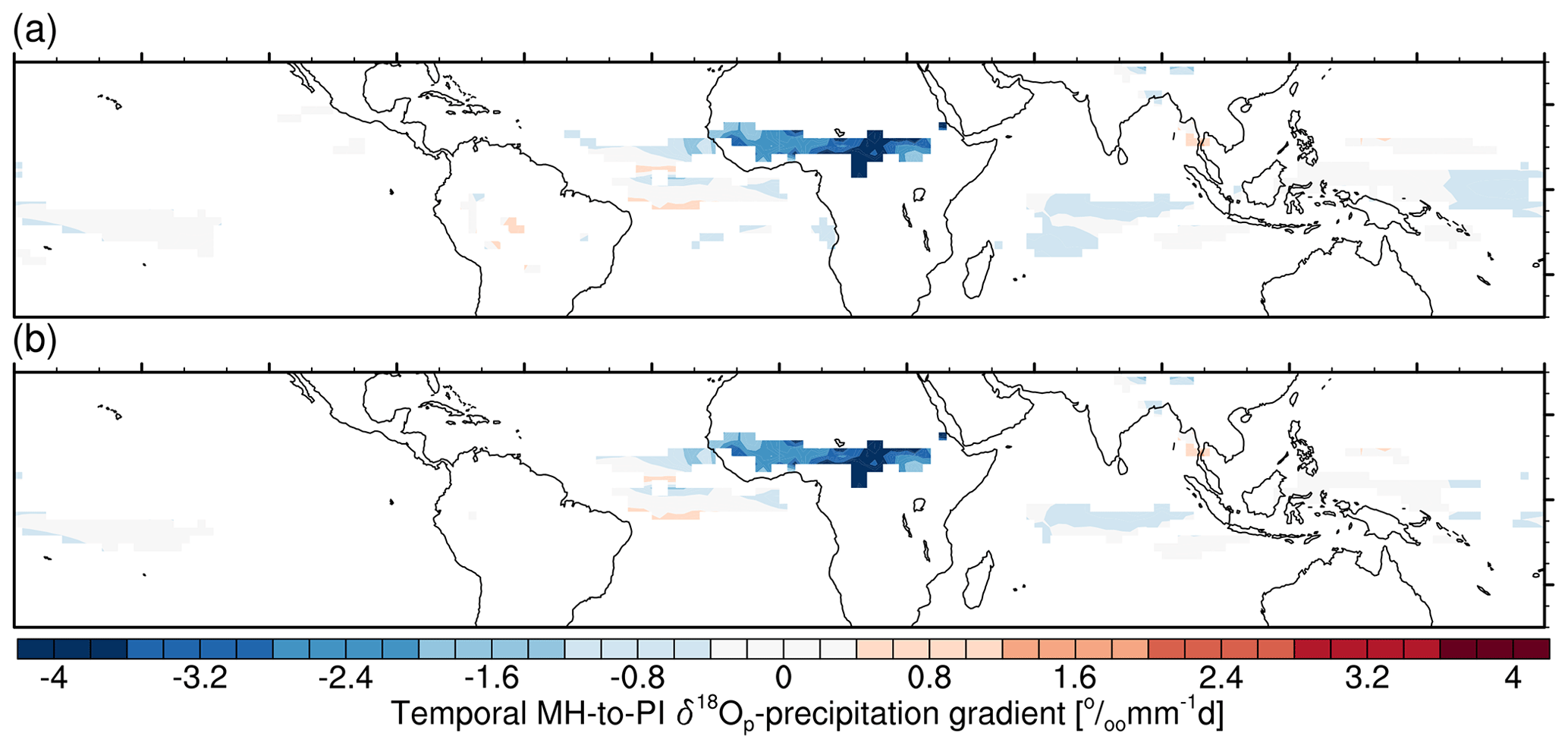
Figure 10 Simulated temporal MH-to-PI δ¹⁸O_p–precipitation gradient for (a) annual mean and (b) JJA mean values. Units: permil per millimeter per day (‰ mm⁻¹ d).

To calculate the MH-to-PI temporal annual mean δ¹⁸O_p–precipitation gradient, we only consider the grid boxes with a substantial precipitation anomaly (larger than 0.5 mm d⁻¹) to ensure a dominate precipitation dependency. Figure 10a presents the distribution map of the temporal gradient between δ¹⁸O_p and total precipitation. The most remarkable feature occurs over the North African monsoon domain, where our model simulates a strong negative δ¹⁸O_p–precipitation gradient up to −4 ‰ mm⁻¹ d, associated with the increased rainfall rate, as shown in Fig. 4a. Our findings are consistent with the so-called amount effect. For other regions, no obvious MH–PI δ¹⁸O_p–precipitation gradient is found. If summer mean δ¹⁸O_p and precipitation are considered instead of the annual mean values, the gradient pattern remains the same (Fig. 10b). This is in contrast to the results of MPI-ESM-wiso which indicate a much steeper gradient for the yearly mean than for the JJA mean values (Cauquoin et al., 2019).

6 Duration of the West African summer monsoon

It is widely believed that the Northern Hemisphere summer monsoon is enhanced in the MH compared to the present day. So far it is unknown whether the wetness in the MH is due to increased precipitation alone or combined with an extension in the monsoon length. Though the monsoon onset has been explored in a great number of studies based on modern observations, there is a lack of knowledge on the initiation date of the MH summer monsoon due to the low temporal resolution in proxy data. In this section for the first time we examine the onset of the mid-Holocene West African summer monsoon (WASM) using the simulated monsoon-related changes in both climatic and isotopic variables (i.e., precipitation, δ¹⁸O_p, and deuterium excess) on a daily scale. The deuterium excess (hereafter referred to as dex) is a second-order isotopic parameter defined as $\mathrm{dex}=\mathit{\delta }D-\mathrm{8}{\mathit{\delta }}^{\mathrm{18}}$O. Changes in dex are often interpreted as a source region effect, namely related to the humidity and temperature conditions in the evaporation source regions (Merlivat and Jouzel, 1979).

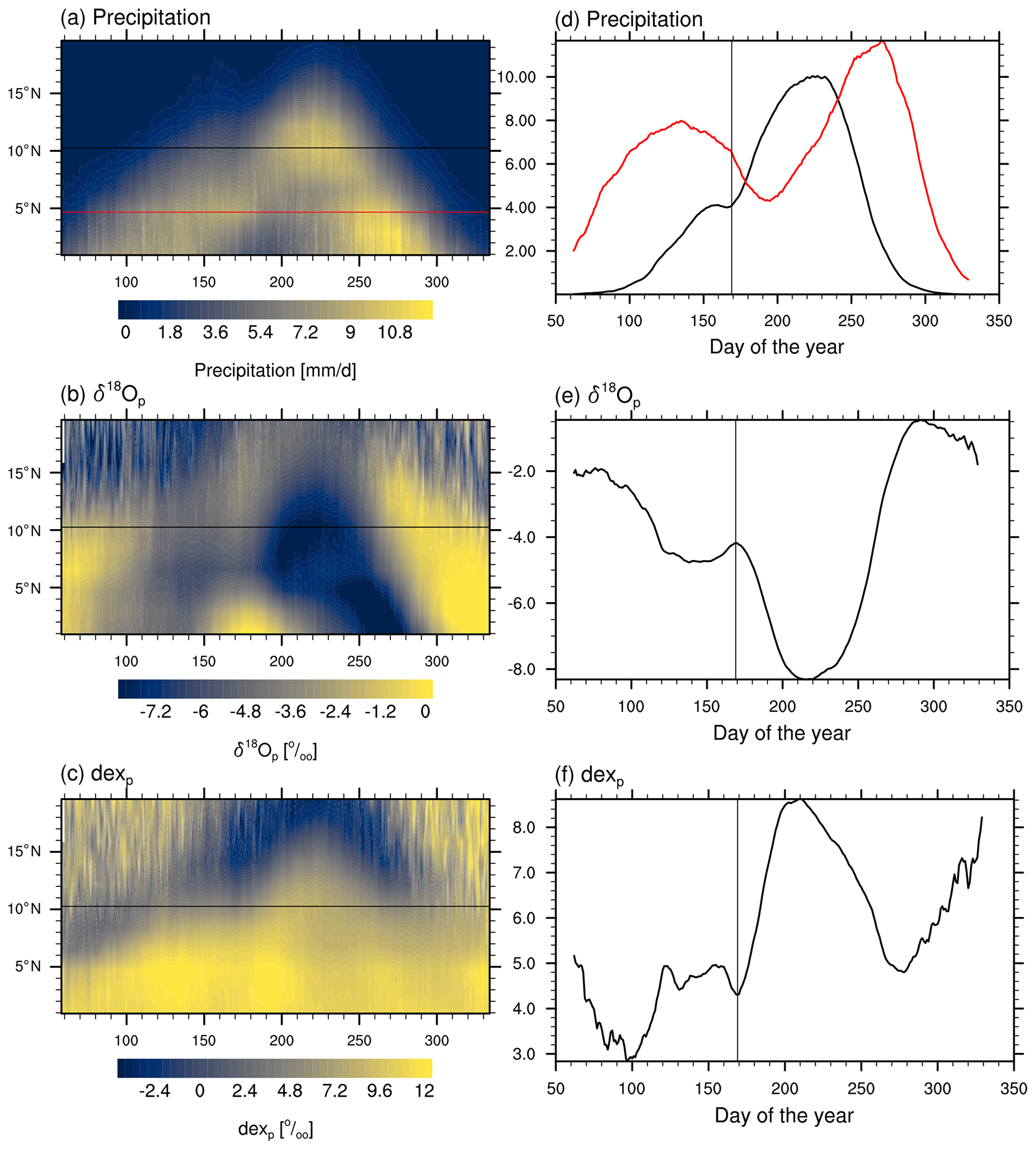
Figure 11 Simulated temporal time–latitude diagram of climatological daily (a) precipitation, (b) δ¹⁸O_p, and (c) dex_p averaged over 15^∘ W–20^∘ E under MH climate conditions, with the x axis representing the day of the year and y axis the latitude. The two black lines correspond to 4.7^∘ N and 10.3^∘ N. (d) Time sections of precipitation averaged over 15^∘ W–20^∘ E at 10.3^∘ N (black line) and at 4.7^∘ N (red line), filtered with high-frequency variability (period less than 10 d) removed. (e, f) Time sections of (e) δ¹⁸O_p and (f) dex_p averaged over 15^∘ W–20^∘ E at 10.3^∘ N, filtered with high-frequency variability (period less than 10 d) removed.

Precipitation on a daily scale is often used for calculating the monsoon onset (e.g., Pausata et al., 2016; Sultan and Janicot, 2003). According to Pausata et al. (2016), the WASM onset is defined as the date preceding the largest increase in precipitation over a 20 d period at the latitude of the maximum in the first empirical orthogonal function (EOF) of the zonally averaged rainfall over the West African monsoon domain (0–20^∘ N, 15^∘ W–20^∘ E). Following Pausata et al. (2016), we first perform an EOF analysis on the zonally averaged daily rainfall data from March to November. As a second step, the latitudinal locations of the maxima of the first two EOFs are computed, representing the ITCZ position during the monsoon and the pre-onset time. The WASM onset occurs in conjunction with a rapid northward shift in the ITCZ. Figure 11a shows a time–latitude diagram of climatological daily precipitation averaged over the West African monsoon domain (0–20^∘ N, 15^∘ W–20^∘ E) under MH climate conditions. The beginning of the WASM leads to a fast increase in precipitation at the northern location of the ITCZ (10.3^∘ N for the MH and 8.4^∘ N for the PI period), as well as a decrease in precipitation at the south location (4.7^∘ N for the MH and 2.8^∘ N for the PI period), a sign of a northward shift in the ITCZ. The monsoon onset is defined as the date preceding the largest increase in precipitation at the northern location over a 20 d period.

Besides daily precipitation, isotope signals also offer an alternative approach to examine the onset of the summer monsoon. The work of Risi et al. (2008) indicates the possibility of detecting the onset of the West African summer monsoon with the use of the isotope composition in precipitation, as the monsoon onset is accompanied by a rapid decrease in δ¹⁸O_p due to intense rainfall, as well as an increase in deuterium excess in precipitation (dex_p) due to reduced re-evaporation of falling rain drops in a humid environment. This phenomenon is also evident in our model. As seen in Fig. 11e and f, the commencement of the WASM is marked by a peak in δ¹⁸O_p and a trough in dex_p. To calculate the monsoon onset, we define I=δ¹⁸O_p − dex_p, and then a peak in I is identifiable when the WASM begins (a typical example shown in Fig. S3). Determining the day when I reaches its peak value from June to July is therefore a straightforward method for determining the onset of the WASM. However, in certain years there are multiple I peaks in June and July (as illustrated in Fig. S4). In order to lessen the overall degree of unpredictability, precipitation can be used as a secondary control. Using combined isotope and precipitation indicators, we propose the following strategy for identifying the WASM onset:

1. Calculate the time series of I and precipitation at the northern latitude of the ITCZ averaged over 15^∘ W–20^∘ E between 1 June and 31 July.

2. Detect the peaks in I.

3. For each day with a I peak, calculate the change in precipitation over the following 20 d.

4. The WASM onset is then defined as the day with the largest increase in precipitation obtained from the previous step.

Due to its continuous and cumulative nature, the isotope composition is a more accurate indicator of the onset of the monsoon in contrast to precipitation, which is typically an individual convection event. As indicated by Risi et al. (2008), the ability of isotope composition in precipitation to document the intra-seasonal regional signal of convective variability is even better than that of the raw local outgoing longwave. Moreover, in our model study, there is a large daily variance in the precipitation over West Africa, leading to occasional difficulty in distinguishing the monsoon season from the pre-onset phase. Two instances are presented here. In the first case (Fig. S5), the precipitation-based method suggests that the WASM commences on the 193rd day of the year (12 July), whereas the decline in isotope index already starts on the 169th day of the year (18 June). An additional example is illustrated in Fig. S6, wherein the precipitation rate experiences a gradual increase over the course of the 50th to 210th day of the year, lacking any abrupt changes. In this instance, identifying the onset of the WASM using solely daily precipitation data is challenging. Therefore, the utilization of isotope tracers can enhance the calculation of the onset date of the summer monsoon in West Africa.

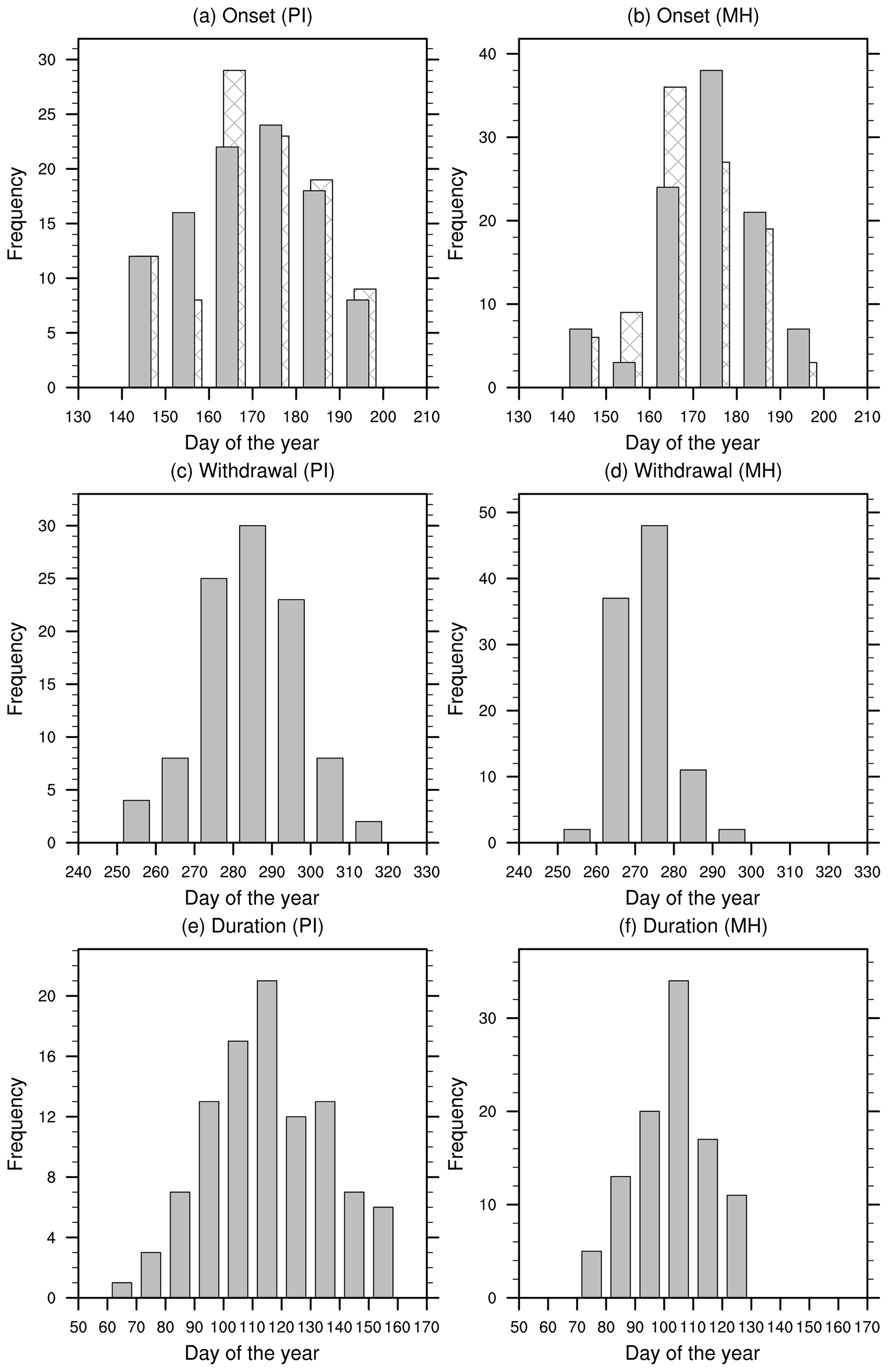
Figure 12 (a, b) Histogram of the WASM onset based on the precipitation approach (solid bars) and isotope approach (stippling bars) for (a) the PI period and (b) the MH. (c, d) Histogram of the WASM withdrawal for (c) the PI period and (d) the MH. (e, f) Same as (c, d) but for the WASM duration.

Analyses of our PI experiment suggest a mean WASM onset date of 19 June based on the isotope approach with a standard deviation of 14 d, and the MH simulation yields a similar result (20 June ± 11 d), indicating that there is no discernible difference between the MH and PI periods in terms of the simulated initiation date of the WASM. The initiation date of the WASM, as determined by precipitation alone, is 21 June ± 15 d for the PI period, similar to the isotope-based approach. For the MH, the precipitation-based method yields a WASM onset date of 23 June ± 12 d. In addition, our histogram plot (i.e., Fig. 12a, b) shows that the WASM onset defined by both approaches is within the 140th to 200th day of the year. Our result also reveals that the onset of the WASM occurs most frequently between the 160th and 180th day of the year.

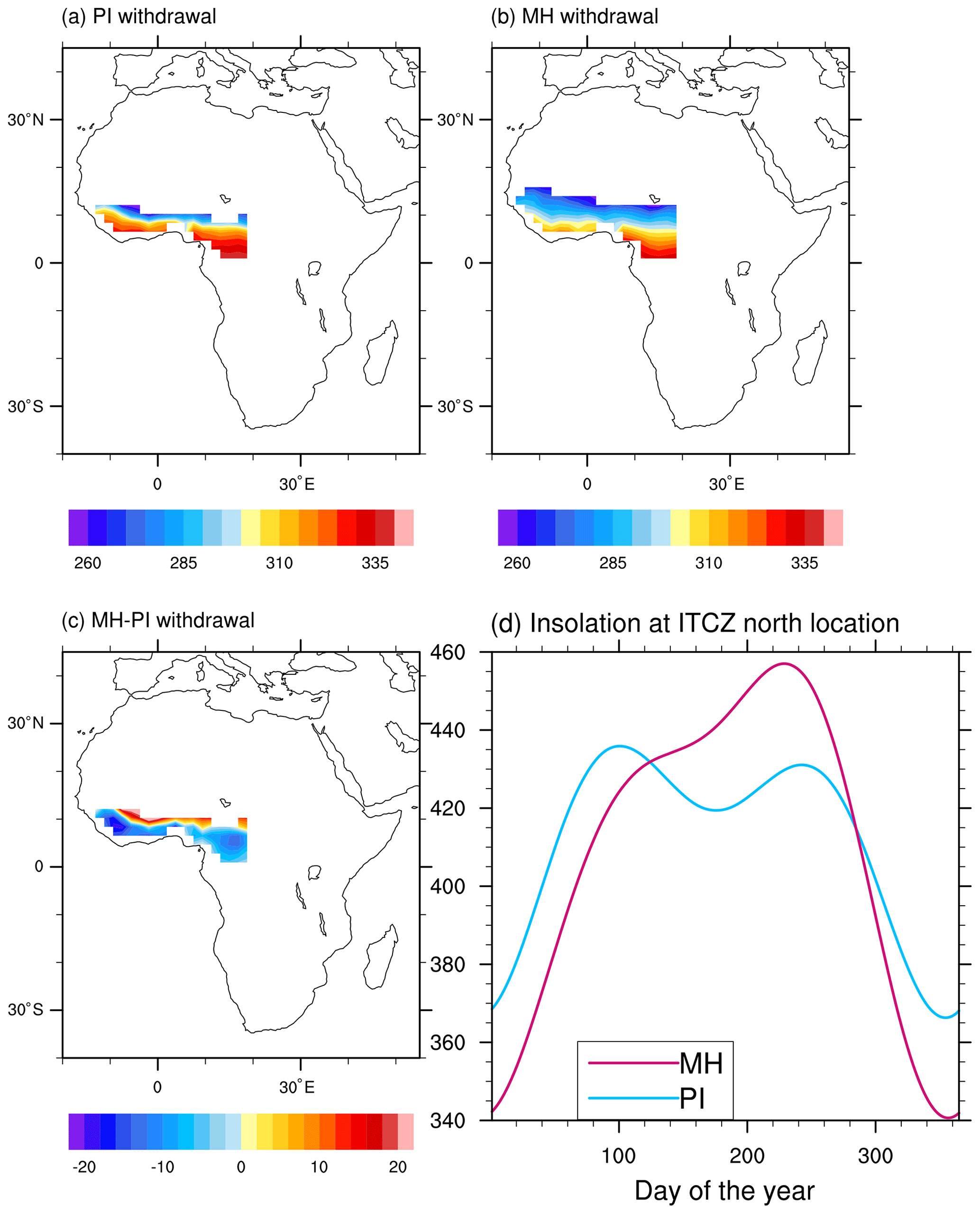
Figure 13 (a–c) Simulated WASM withdrawal date for (a) PI, (b) MH, and (c) MH–PI. (d) Time series of insolation averaged over 15^∘ W–20^∘ E at the northern location of the ITCZ for both the PI and MH periods.

With respect to the withdrawal of the WASM, we exclusively employ the daily precipitation time series. According to Pausata et al. (2016), we define the WASM withdrawal as the date on which the zonally averaged precipitation at the northern latitude of the ITCZ falls below 2 mm d⁻¹ for at least 20 consecutive days. The monsoon’s duration is simply computed as the time interval between its onset and withdrawal. Based on this approach, the calculated WASM withdrawal is 10 October and 29 September for the PI and MH periods, with a standard deviation of 13 and 7 d, respectively. Thus the duration of the WASM is 113 d for the PI period and 101 d for the MH, indicating a shorter WASM season in the MH than in the PI period. In the PI period, the retreat of the summer monsoon over West Africa is most frequently observed within the 270th to 300th day of the year (27 September to 27 October) (Fig. 12c, d), while in most model years, the WASM in the MH terminates within the 260th to 280th day of the year (17 September to 7 October). The duration of the WASM in the PI period can reach up to 160 d, whereas for the MH the maximum WASM length is only 130 d (Fig. 12e, f). Furthermore, following D'Agostino et al. (2019), we define the WASM domain as the area where the precipitation anomaly between the JJAS and DJFM seasons exceeds 2 mm d⁻¹. To examine the retreat of the summer monsoon on a local scale, we further calculate the termination date of the WASM for each grid box within the monsoon domain. As depicted in Fig. 13a and b, the termination of the rainy season exhibits a meridional distribution, driven by the shift in maximum insolation. We also observe an earlier withdrawal of the WASM in most parts of the monsoon domain, particularly in the southern region (Fig. 13c). Additionally, the shorter duration of the MH WASM can be attributed to a more rapid decrease in insolation at the northern location of the ITCZ in the MH compared to the PI period. Our result indicates that the simulated intensification in the MH WASM is attributable to a rise in precipitation rate alone rather than an extension of the monsoon season.

Our investigation on the WASM onset, retreat, and duration can be treated as a case study of model data application, which may help shed light on how we can use model variables with daily frequency to examine synoptic climatic processes. On the basis of model simulations with stable isotope diagnostics, we show here the potential of enhancing the precipitation-based technique with the additional use of isotope composition to detect the arrival of past summer monsoons. However, as proxy-based reconstructions cannot resolve daily variations in precipitation or water isotopes, such an analysis can only be achieved with the use of daily model variables. Moreover, as the lengths of months and seasons are different between MH and PI angular calendars (Shi et al., 2022a), the date of the WASM onset and withdrawal in this section is based only on a modern classical calendar. We keep in mind that there is a constant shift between the two types of calendars by 1–3 d for the PI and MH periods (Shi et al., 2022a); however, this effect is neglectable given the large variance of the onset and withdrawal of the WASM.

7 Discussion

In this study we have evaluated the performance of AWI-ESM-2.1-wiso in simulating the pre-industrial isotope characteristics by a comparison to modern measurements and a marine δ¹⁸O reanalysis dataset produced by Breitkreuz et al. (2018a).

Our modeled PI δ¹⁸O_p agrees well with the observation data, not only for (sub-)tropical and midlatitude areas but even for the polar regions where temperatures fall below −20 ^∘C. These regions have been a major challenge for isotope-enabled models in terms of reproducing correctly the isotope composition in precipitation and surface snow. Using a coarse-resolution atmosphere model, Werner et al. (2011) obtained an enrichment bias in δ¹⁸O_p across Antarctic ice core locations, mostly linked to an overestimation of Antarctic temperatures. This bias did not improve by coupling the model to the ocean model MPIOM (Werner et al., 2016). The use of a coarse model resolution is a possible reason for this model–data mismatch. An upgraded model version with higher spatial and vertical resolution for the atmosphere decreased the bias in simulated δ¹⁸O_p over Antarctica, but the modeled values still deviated clearly from observations (Cauquoin et al., 2019). With the use of AWI-ESM-2.1-wiso in our study, we obtain a good model–data agreement over Antarctica, even for the ice core locations with temperatures lower than −50 ^∘C. This is a significant improvement compared to results with earlier models equipped with water isotopes.

Compared to marine δ¹⁸O reanalysis data (Breitkreuz et al., 2018a), our model produces isotopically more depleted Arctic surface seawater for the PI period. However, we should keep in mind that the marine δ¹⁸O reanalysis data at the surface level of the Arctic Ocean may be biased because the influence of isotopically highly depleted precipitation is not preserved in the sea ice model used for the assimilation, as pointed out by Breitkreuz et al. (2018a). The enrichment bias of δ¹⁸O_oce in the Antarctic bottom water in our PI simulation results from an overestimation of δ¹⁸O_oce in the Southern Ocean surface water. However, our PI simulation is constrained by the boundary conditions of 1850 CE, whereas the dataset used for comparison was generated based on an ocean general circulation model constrained by δ¹⁸O_oce data collected from 1950 to 2011 and climatological salinity and temperature data collected from 1951 to 1980. Due to the rise in greenhouse gases after 1850, enhanced melting of ice shelves may have occurred (Rintoul, 2007), which could result in an isotopically more depleted Southern Ocean.

For the mid-Holocene, AWI-ESM-2.1-wiso simulates enhanced seasonality in surface air temperature and increased precipitation across the monsoon areas of the Northern Hemisphere, compared to the pre-industrial period. For assessing the modeled MH-minus-PI isotope anomalies, reconstructions derived from ice cores, speleothems, and multiple species of planktonic foraminifera are used. Our model captures the signs in the reconstructed MH-minus-PI δ¹⁸O in precipitation and seawater well, however, with a much narrower range. Upon comparing model and data, we also discover inconsistencies in certain locations. The mismatch between simulated and observed isotope signals might be attributable to either model bias or data uncertainties. Compared to pollen-based reconstructions, our modeled MH–PI anomalies in temperature and precipitation are less pronounced (Bartlein et al., 2011; Shi et al., 2022b), which tends to leave a weak imprint on the simulated isotope changes. Moreover, our MH simulation differs from the PI one only for the insolation and greenhouse forcings, but in reality other elements (e.g., lakes, vegetation, volcanoes, ozone, or the ecosystem) also play important roles. Model resolution is another key factor affecting the simulated result (Werner et al., 2011). On the other hands, there are also uncertainties in the reconstructed data. For instance, ice core records are also influenced by the seasonality or intermittency of precipitation (Werner et al., 2000). δ¹⁸O_p signals documented in speleothems may result from a complicated interplay of localized environmental processes (Lachniet, 2009). In addition, foraminifera in cold areas are more likely to record summer δ¹⁸O_oce values (e.g., Jonkers and Kučera, 2015).

Our analysis of the MH-to-PI temporal gradient between δ¹⁸O_p and temperature indicates that the MH-to-PI temporal ratio of δ¹⁸O_p to surface air temperature is reasonable over Greenland and Antarctica only when summertime air temperature is considered. Our results suggest that the spatial δ¹⁸O_p–T slope observed under the modern climate could be a surrogate for the MH-to-PI temporal isotope–temperature gradient during the warmest month/season over Greenland and Antarctica, consistent with a previous study using MPI-ESM-wiso (Cauquoin et al., 2019). Nevertheless, this conclusion might be model-dependent, since both MPI-ESM-wiso and AWI-ESM-2.1-wiso use the same atmospheric model, ECHAM6-wiso. Therefore, further analyses of the different slopes by using other isotope-enabled models would be advantageous.

Since the onset of the summer monsoon is accompanied by a rapid increase in rainfall, the daily precipitation is often used to define the monsoon onset (Sultan and Janicot, 2003; Dunning et al., 2016). Other studies have used the surface outgoing longwave radiation (Fontaine et al., 2008; Chenoli et al., 2018; Bhatla et al., 2016) and the low-level zonal wind (Wang et al., 2004; Zhang, 2010) for this purpose. In addition to climatic variables, isotope signals offer an alternative approach to examine the onset of the Northern Hemisphere summer monsoon. The validity of δ¹⁸O_p to study Indian monsoon onsets has been supported by Yang et al. (2012). Earlier studies of the δ¹⁸O_p over South Asia have shown a coincidence of a dramatic decrease in δ¹⁸O_p with monsoon onset (Tian et al., 2001; Vuille et al., 2005). Moreover, Risi et al. (2008) have revealed that, during the African monsoon onset, the abrupt increase in convective activity over the Sahel is associated with an abrupt decrease in δ¹⁸O_p, as well as an increase in deuterium excess in precipitation. Our results are in line with these findings and suggest that combining signals from isotope and precipitation could enhance the definition of the WASM onset.

8 Conclusions

In the present study we report the first results of two equilibrium simulations performed under both PI and MH boundary conditions using a newly developed coupled climate model equipped with water stable isotopes, named AWI-ESM-2.1-wiso. For the PI period, we provide a model evaluation for the simulated isotope composition in precipitation and ocean surface water versus various sources of observations. Our modeled δ¹⁸O_p values are in good agreement with GNIP and ice core measurements. The global distributions of δ¹⁸O_oce of the surface water and the zonal mean δ¹⁸O_oce in Atlantic and Pacific sections produced by our model show great similarity to marine δ¹⁸O reanalysis data by Breitkreuz et al. (2018a).

Our model results in terms of the climate changes between the MH and PI periods are in line with PMIP4 models (Brierley et al., 2020), showing an enhanced seasonality in surface temperature which is driven by the redistribution of seasonal insolation and an increase in Northern Hemisphere monsoonal rainfall governed by a northward shift in the Intertropical Convergence Zone (ITCZ). The MH–PI differences in temperature and precipitation give rise to important changes in isotope signal on a global scale. More enriched δ¹⁸O_p is simulated over the Arctic Ocean and Greenland due to summer warming, as well as over the western tropical Pacific led by decreased precipitation amount. Enhanced monsoonal rainfall over North Africa favors a pronounced decrease in isotope composition. Our simulated MH–PI anomalies in δ¹⁸O_p are fairly consistent with speleothem and ice core reconstructions, though model–data mismatch can be found in certain regions (e.g., part of South America and East Antarctica). For the subtropical areas, isotopic compositions archived in speleothems might reflect very localized processes related to the cave environment which are hard to capture in model simulations.

Analysis of the simulated isotope–temperature relationship reveals a stable spatial δ¹⁸O_p–T gradient across the MH and PI periods. On a global scale, the modeled spatial gradient (0.71 ‰ ^∘C⁻¹ for both the PI and MH periods) is comparable to the observed value (0.69 ‰ ^∘C⁻¹) (Dansgaard, 1964). This coefficient, however, may vary from region to region in response to a number of meteorological factors. Therefore, for meaningful reconstructions of past climate changes in a given area, attempts should be made to validate the local δ¹⁸O_p–temperature gradient at the time of interest (Fricke and O'Neil, 1999). In the present study we calculate the MH-to-PI temporal gradient between δ¹⁸O_p and temperature and find that the gradient over Greenland and Antarctica can become reasonable only if the variables are derived from the warmest month of the year. This result is consistent with the findings of Cauquoin et al. (2019). Furthermore, a clear amount effect is reflected in the temporal δ¹⁸O_p–precipitation relationship over the North African monsoon region, as a pronounced depletion in δ¹⁸O_p is found in response to increased monsoonal rainfall.

Numerous studies have investigated the onset and withdrawal of the modern summer monsoon over West Africa, but for the mid-Holocene corresponding studies are lacking as the temporal resolutions of most proxy records are insufficient for such an analysis. Paleoclimate model simulations may provide an alternative approach to investigate the onset and termination of past monsoon events. In this work, we evaluate the onset, termination, and duration of the MH WASM based on both simulated daily variables. We propose a new method for defining the WASM onset using δ¹⁸O_p, dex_p, and precipitation rate at a daily scale. Our simulations show that there has been no obvious difference in the WASM onset between the MH and PI periods. However, we observe a significant advancement in the withdrawal of the MH WASM compared to the PI period. Our analysis suggest that the simulated intensification in the MH WASM is mainly attributable to a strengthening in rainfall rate rather than an extension of the monsoon duration.