A method to derive Fourier–wavelet spectra for the characterization of global-scale waves in the mesosphere and lower thermosphere and its MATLAB and Python software (fourierwavelet v1.1)

This paper describes a simple method for characterizing global-scale waves in the mesosphere and lower thermosphere (MLT), such as tides and traveling planetary waves, using uniformly gridded two-dimensional longitude–time data. The technique involves two steps. In the first step, the Fourier transform is performed in space (longitude), and then the time series of the space Fourier coefficients are derived. In the second step, the wavelet transform is performed on these time series, and wavelet coefficients are derived. A Fourier–wavelet spectrum can be obtained from these wavelet coefficients, which gives the amplitude and phase of the wave as a function of time and wave period. It can be used to identify wave activity that is localized in time, similar to a wavelet spectrum, but the Fourier–wavelet spectrum can be obtained separately for eastward- and westward-propagating components and for different zonal wavenumbers. The Fourier–wavelet analysis can be easily implemented using existing Fourier and wavelet software. MATLAB and Python scripts are created and made available at https://igit.iap-kborn.de/yamazaki/fourierwavelet (last access: 18 August 2023) that compute Fourier–wavelet spectra using the wavelet software provided by Torrence and Compo (1998). Some application examples are presented using MLT data from atmospheric models.

1 Introduction

1.1 Background and motivation

The Earth's atmosphere can support various types of global-scale waves, which zonally extend around a full circle of latitude. The zonal wavenumber is defined as the number of wave cycles that fit within the latitude circle. As the wave propagates eastward or westward, an oscillation is observed at ground stations. The period of the oscillation depends on the zonal phase velocity and zonal wavenumber of the wave,

$$\begin{array}{}\text{(1)}& T={\mathit{\omega }}^{-\mathrm{1}}={\displaystyle \frac{\mathrm{2}\mathit{\pi }{R}_{\mathrm{E}}}{kC}}\cos \mathit{\varphi },\end{array}$$

where T (in seconds) is the wave period, ω (in s⁻¹) is the wave frequency, R_E (in m) is the Earth's radius, k is the zonal wavenumber, C (in m s⁻¹) is the phase speed, and ϕ (in rad) is the latitude.

Examples of global-scale waves in the atmosphere include atmospheric tides (Lindzen and Chapman, 1969; Forbes, 1984) and traveling planetary waves (Salby, 1984; Madden, 2007). Solar tides, with primary periods at 24 and 12 h (called diurnal and semidiurnal tides, respectively), are thermally excited through periodic absorption of solar radiation mainly in the troposphere and stratosphere (Forbes, 1982a, b). Dominant modes are the westward-propagating migrating (or sun-synchronous) diurnal tide with zonal wavenumber 1 (DW1) and the migrating semidiurnal tide with zonal wavenumber 2 (SW2). Besides, non-migrating (or non-sun-synchronous) modes are also commonly observed, such as eastward-propagating diurnal tides with zonal wavenumber 3 (DE3) and wavenumber 2 (DE2; e.g., Hagan and Forbes, 2002; Forbes et al., 2008; Oberheide et al., 2011). Tides propagate vertically upward from the source region. Their amplitude increases with height due to the reduction in the atmospheric density until dissipation eventually takes place in the mesosphere and lower thermosphere (MLT) and prevents their further growth. As a result, the wave amplitude is often largest in the MLT region.

Traveling planetary waves have a period longer than a day and shorter than several weeks. Some are interpreted as normal modes, which are predicted by classical linear wave theory (e.g., Longuet-Higgins, 1968; Kasahara, 1976). Normal modes are solutions to Laplace's tidal equation in an idealized atmosphere with no dissipation and mean winds and represent free (or resonant) oscillations of the atmosphere (Forbes, 1995). Global characteristics of normal modes can be predicted based on the linear wave theory (Kasahara and Puri, 1981; Žagar et al., 2015; Marques et al., 2020). Spectral analysis of meteorological data has confirmed the existence of waves similar to those theoretically predicted in the troposphere and stratosphere (e.g., Madden, 2007; Sakazaki and Hamilton, 2020). However, characteristics of traveling planetary waves in the MLT region are expected to deviate considerably from those of theoretical normal modes due, for example, to dissipation and mean winds (Salby, 1981c). Also, some traveling planetary waves in the MLT region are considered to be unstable modes locally generated by atmospheric instability rather than normal modes (e.g., Pfister, 1985; Meyer and Forbes, 1997).

Traveling planetary waves that are most commonly observed in the MLT region have periods of about 5–7 d (Hirota and Hirooka, 1984; Wu et al., 1994; Forbes and Zhang, 2017; Qin et al., 2021c), 9–11 d (Hirooka and Hirota, 1985; Forbes and Zhang, 2015), and 14–16 d (Forbes et al., 1995a; Day et al., 2011). They are all westward-propagating, with zonal wavenumber 1, and called quasi-6 d wave (Q6DW), quasi-10 d wave (Q10DW), and quasi-16 d wave (Q16DW), respectively. The zonal wavenumber and wave period of these waves are consistent with Rossby modes of the linear wave theory, but their meridional and vertical structures are generally different from those of theoretical Rossby modes. This is also the case for the westward-propagating quasi-28 d wave (Q28DW) with zonal wavenumber 1 (Zhao et al., 2019), the westward-propagating quasi-4 d wave (Q4DW) with zonal wavenumber 2 (Ma et al., 2020; Yamazaki et al., 2021), and the westward-propagating quasi-7 d wave (Q7DW) with zonal wavenumber 2 (Pogoreltsev et al., 2002). The westward-propagating quasi-2 d wave (Q2DW) with zonal wavenumber 2–4 is frequently observed in the MLT region (Wu et al., 1993; Gu et al., 2013; Moudden and Forbes, 2014; He et al., 2021) and is sometimes regarded as a manifestation of mixed Rossby–gravity modes (e.g., Salby, 1981a; Salby and Callaghan, 2001). Although theoretical Rossby and mixed Rossby–gravity modes are westward-propagating waves, observations sometimes show eastward-propagating waves around the same period range (e.g., Palo et al., 2007; McDonald et al., 2011; Pancheva et al., 2018; Huang et al., 2021; Fan et al., 2022; Luo et al., 2023). Observations also sometimes show westward-propagating planetary waves in the MLT region for which the periods do not match those of normal modes (e.g., Qin et al., 2022a, 2021b). Equatorial Kelvin waves (Matsuno, 1966; Holton and Lindzen, 1968) are equatorially trapped eastward-propagating waves. At MLT heights, the ultra-fast Kelvin wave (UFKW) with zonal wavenumber 1 and a period of ∼ 3 d is frequently detected (e.g., Lieberman and Riggin, 1997; Forbes et al., 2009; Davis et al., 2012; Gasperini et al., 2015, 2018; Yamazaki et al., 2020b).

Neither tides nor traveling planetary waves are stationary. Generally, their amplitude varies with season. Besides, tidal amplitude shows marked day-to-day variability in the MLT region (e.g., Miyoshi and Fujiwara, 2003; Pedatella et al., 2012a; Wang et al., 2021b; Zhou et al., 2022). This can be attributed to the interaction of tidal waves with the mean flow and other waves (e.g., Chang et al., 2011; Lieberman et al., 2015; Siddiqui et al., 2022), as well as to changes in the source of tides (e.g., Miyoshi, 2006; Siddiqui et al., 2019). Traveling planetary waves in the MLT region sometimes show a burst of wave activity that lasts for a few wave cycles. This can result from changes in the zonal mean state of the atmosphere, which controls propagation conditions, atmospheric instability, and critical layers (e.g., Salby, 1981b, c; Liu et al., 2004; Yue et al., 2012; Gan et al., 2018). A wave burst is often observed around seasonal transition, but its characteristics (e.g., magnitude, peak period, meridional structure, and so on) vary from year to year, so that it is difficult to predict them (e.g., Gu et al., 2019; Liu et al., 2019; Yamazaki et al., 2021). Also, some wave burst events occur during sudden stratospheric warmings.

A sudden stratospheric warming is a large-scale meteorological disturbance, which usually takes place in the winter polar stratosphere (e.g., Butler et al., 2015; Baldwin et al., 2021). It can influence the whole atmosphere, including different latitudes and heights (e.g., Pedatella et al., 2018; Goncharenko et al., 2021). As the mean state of the stratosphere and mesosphere is considerably altered during a sudden stratospheric warming, changes may occur in the amplitude and phase of tides and traveling planetary waves. Numerical studies have predicted changes in tides in the MLT region during sudden stratospheric warmings (e.g., Stening et al., 1997; Fuller-Rowell et al., 2010; Pedatella et al., 2012b; Jin et al., 2012; Siddiqui et al., 2018). Indeed, marked tidal changes have been observed in the MLT region during sudden stratospheric warmings (e.g., Sridharan et al., 2009; Xiong et al., 2013; Zhang and Forbes, 2014; Hibbins et al., 2019; Stober et al., 2020; Liu et al., 2022). Also, the large amplification of traveling planetary waves is sometimes observed in the MLT region following sudden stratospheric warming events (e.g., Espy et al., 2005; Matthias et al., 2012; Sassi et al., 2012; Chandran et al., 2013; Gu et al., 2016; Yamazaki and Matthias, 2019; He et al., 2020b, a; Wang et al., 2021a).

Understanding wave activity in the MLT region is important because it has a significant impact on the region above, i.e., the ionosphere and thermosphere (IT; e.g., Liu, 2016; Yiğit and Medvedev, 2015). The IT region is where many space infrastructures operate and is important for radio communication between the ground stations and satellites (Schunk and Sojka, 1996; Moldwin, 2022). Many studies have found wave-like signatures in the IT region that correlate with tidal and traveling planetary wave activity in the MLT region (e.g., Laštovička, 2006; Immel et al., 2006; Oberheide et al., 2009; Pancheva and Mukhtarov, 2010; Gu et al., 2014; Yamazaki, 2018; Gan et al., 2020; Sobhkhiz-Miandehi et al., 2022).

Characterization of global-scale waves requires the identification of the zonal wavenumber and wave period (see Eq. 1), which demands two-dimensional (2-D) spatiotemporal data (more specifically, data as a function of longitude and time). Techniques such as 2-D fast Fourier transform (FFT; e.g., Hayashi, 1971) and the 2-D least squares fitting method (e.g., Wu et al., 1995) can be applied to the data to evaluate the zonal wavenumber and wave period of global-scale waves and their amplitudes and phases. Taking into account the transient nature of global-scale waves in the MLT region, a short-time analysis is commonly used. That is, a 2-D spectral analysis is performed on a short-time segment of the data, and then the analysis window is moved forward in time (e.g., Maute, 2017; Forbes et al., 2018; Liu et al., 2021). In this way, it is possible to evaluate temporal variations in the global-scale waves. However, such a moving window approach is computationally expensive because the spectral analysis needs to be repeated multiple times. As a solution to this problem, this study proposes the application of wavelet analysis. The wavelet analysis (e.g., Mallat, 1999) is a multiresolution analysis technique using a “wavelet”, which is a short-term-duration wave. A wavelet transform can be performed on one-dimensional (1-D) time series to derive a “wavelet spectrum”, which is usually presented in a time versus period diagram. The wavelet spectrum is useful for identifying wave activity that is localized in time. The wavelet algorithm avoids the use of a moving window, which makes the technique more computationally efficient than the short-time analysis. The main objectives of this study are (1) to introduce a simple method to derive “wavelet-like” spectra from 2-D longitude–time data, which can be used for the characterization of global-scale waves in the MLT region, and (2) to deliver easy-to-use software in two user-friendly languages, namely MATLAB and Python. For (1), the 2-D FFT method of Hayashi (1971) is used, and it is modified by adopting the wavelet technique described by Torrence and Compo (1998). The Hayashi (1971) method is easy to implement, and its spectrum directly gives the wave amplitude in units of the input data, which is easy to interpret.

1.2 Fourier-based analysis of space–time data

Hayashi (1971) proposed a Fourier-based spectral analysis method for 2-D longitude–time data, which was successfully implemented in later studies (e.g., Mechoso and Hartmann, 1982; Wheeler and Kiladis, 1999; Miyoshi and Fujiwara, 2006; Akmaev et al., 2008; Sassi et al., 2016). The technique involves two steps. In the first step, the Fourier transform is performed in space (longitude), and the time series of the sine and cosine Fourier coefficients are derived. In the second step, the Fourier transform is performed on these time series. Hayashi (1971) clarified how the amplitude and phase of eastward- and westward-propagating waves are related to the Fourier coefficients obtained from the second Fourier transform. What follows is a brief review of the technique of Hayashi (1971).

Assuming that the perturbations of an atmospheric variable W (denoted by δW) at a fixed latitude can be expressed as the sum of eastward- and westward-propagating components with various zonal wavenumbers k (=0, 1, 2, …) and frequencies ω ($>\mathrm{0};={\mathit{\omega }}_{\mathrm{0}}$, ω₁, ω₂, …),

$$\begin{array}{}\text{(2)}& \mathit{\delta }W=\sum _k\mathit{\delta }{W}_k=\sum _k\left(\mathit{\delta }{W}_k^{+}+\mathit{\delta }{W}_k^{-}\right),\end{array}$$

where

$$\begin{array}{}\text{(3)}& \mathit{\delta }{W}_k^{+}=\sum _{\mathit{\omega }}{R}_{k,\mathit{\omega }}^{+}\cos \left(\mathit{\omega }t-k\mathit{\lambda }-{\mathit{\phi }}_{k,\mathit{\omega }}^{+}\right)\end{array}$$

represents eastward-propagating components, and

$$\begin{array}{}\text{(4)}& \mathit{\delta }{W}_k^{-}=\sum _{\mathit{\omega }}{R}_{k,\mathit{\omega }}^{-}\cos \left(\mathit{\omega }t+k\mathit{\lambda }-{\mathit{\phi }}_{k,\mathit{\omega }}^{-}\right)\end{array}$$

is the westward-propagating counterpart. t and λ are time (in seconds) and longitude (in rad), respectively. R and φ are the amplitude and phase of the wave component, respectively, with the superscripts + and − indicating the eastward- and westward-propagating components, respectively. The above equations can be rearranged, and the component with zonal wavenumber k can be written as

$$\begin{array}{}\text{(5)}& \mathit{\delta }{W}_k=C_k\left(t\right)\cos kx+S_k\left(t\right)\sin kx,\end{array}$$

with

$$\begin{array}{}\text{(6)}& {\displaystyle }& {\displaystyle }{C}_k\left(t\right)=\sum _{\mathit{\omega }}\left(A_{k,\mathit{\omega }}\cos \mathit{\omega }t+B_{k,\mathit{\omega }}\sin \mathit{\omega }t\right)\text{(7)}& {\displaystyle }& {\displaystyle }{S}_k\left(t\right)=\sum _{\mathit{\omega }}\left(a_{k,\mathit{\omega }}\cos \mathit{\omega }t+b_{k,\mathit{\omega }}\sin \mathit{\omega }t\right),\end{array}$$

where

$$\begin{array}{}\text{(8)}& {\displaystyle }& {\displaystyle }{A}_{k,\mathit{\omega }}=R_{k,\mathit{\omega }}^{+}\cos {\mathit{\phi }}_{k,\mathit{\omega }}^{+}+R_{k,\mathit{\omega }}^{-}\cos {\mathit{\phi }}_{k,\mathit{\omega }}^{-}\text{(9)}& {\displaystyle }& {\displaystyle }{B}_{k,\mathit{\omega }}=R_{k,\mathit{\omega }}^{+}\sin {\mathit{\phi }}_{k,\mathit{\omega }}^{+}+R_{k,\mathit{\omega }}^{-}\sin {\mathit{\phi }}_{k,\mathit{\omega }}^{-}\text{(10)}& {\displaystyle }& {\displaystyle }{a}_{k,\mathit{\omega }}=-R_{k,\mathit{\omega }}^{+}\sin {\mathit{\phi }}_{k,\mathit{\omega }}^{+}+R_{k,\mathit{\omega }}^{-}\sin {\mathit{\phi }}_{k,\mathit{\omega }}^{-}\text{(11)}& {\displaystyle }& {\displaystyle }{b}_{k,\mathit{\omega }}=R_{k,\mathit{\omega }}^{+}\cos {\mathit{\phi }}_{k,\mathit{\omega }}^{+}-R_{k,\mathit{\omega }}^{-}\cos {\mathit{\phi }}_{k,\mathit{\omega }}^{-}.\end{array}$$

Equations (8)–(11) can be further rearranged as follows:

$$\begin{array}{}\text{(12)}& {\displaystyle }& {\displaystyle }{R}_{k,\mathit{\omega }}^{\pm }\cos {\mathit{\phi }}_{k,\mathit{\omega }}^{\pm }={\displaystyle \frac{\mathrm{1}}{\mathrm{2}}}\left(A_{k,\mathit{\omega }}\pm b_{k,\mathit{\omega }}\right)\text{(13)}& {\displaystyle }& {\displaystyle }{R}_{k,\mathit{\omega }}^{\pm }\sin {\mathit{\phi }}_{k,\mathit{\omega }}^{\pm }={\displaystyle \frac{\mathrm{1}}{\mathrm{2}}}\left(B_{k,\mathit{\omega }}\mp a_{k,\mathit{\omega }}\right),\end{array}$$

from which R and φ can be derived as

$$\begin{array}{}\text{(14)}& {\displaystyle }& {\displaystyle }{R}_{k,\mathit{\omega }}^{\pm }={\displaystyle \frac{\mathrm{1}}{\mathrm{2}}}\sqrt{{\left(A_{k,\mathit{\omega }}\pm b_{k,\mathit{\omega }}\right)}^{\mathrm{2}}+{\left(B_{k,\mathit{\omega }}\mp a_{k,\mathit{\omega }}\right)}^{\mathrm{2}}}\text{(15)}& {\displaystyle }& {\displaystyle }{\mathit{\phi }}_{k,\mathit{\omega }}^{\pm }=\arctan {\displaystyle \frac{B_{k,\mathit{\omega }}\mp a_{k,\mathit{\omega }}}{A_{k,\mathit{\omega }}\pm b_{k,\mathit{\omega }}}}.\end{array}$$

$R_{k,\mathit{\omega }}^{\pm }$ and ${\mathit{\phi }}_{k,\mathit{\omega }}^{\pm }$ can be determined using longitude–time data sampled at a fixed latitude by first performing the Fourier transform in longitude to obtain time series of the sine and cosine Fourier coefficients (i.e., S_k(t) and C_k(t)) and then performing the Fourier transform on S_k(t) and C_k(t) to obtain the sine and cosine Fourier coefficients (i.e., B_k,ω, b_k,ω, A_k,ω, and a_k,ω).

1.3 Wavelet analysis of time series

A wavelet analysis is performed in time. The method considered here is the continuous wavelet transform described by Torrence and Compo (1998). Their wavelet software, including the software in MATLAB and Python, is available online (http://atoc.colorado.edu/research/wavelets/, last access: 18 August 2023) and is widely used in atmospheric science due to the ease of use. Below, the technique described by Torrence and Compo (1998) is only briefly summarized. Readers are referred to Torrence and Compo (1998) for full details.

For a given time series x(t), the continuous wavelet transform X is defined as the convolution of x(t) with a wavelet function Ψ as follows:

$$\begin{array}{}\text{(16)}& X(s,\mathit{\tau })=\underset{-\mathrm{\infty }}{\overset{\mathrm{\infty }}{\int }}x\left(t\right){\mathrm{\Psi }}^{*}\left({\displaystyle \frac{t-\mathit{\tau }}{s}}\right)\mathrm{d}t,\end{array}$$

where s is the scaling factor, representing the extent of dilation or compression of the wavelet, and τ is the translation factor, representing time shift. Ψ^* is the complex conjugate of Ψ. For the present study, the Morlet wavelet is used for Ψ. The Morlet wavelet is the product of a complex sinusoid and a Gaussian window. That is,

$$\begin{array}{}\text{(17)}& \mathrm{\Psi }\left({\displaystyle \frac{t}{s}}\right)=\left(\cos {\displaystyle \frac{{\mathit{\omega }}_{\mathrm{0}}t}{s}}+i\sin {\displaystyle \frac{{\mathit{\omega }}_{\mathrm{0}}t}{s}}\right)e^{-\frac{\mathrm{1}}{\mathrm{2}}{\left(\frac{t}{s}\right)}^{\mathrm{2}}}.\end{array}$$

ω₀ is usually set to be 6 to satisfy the admissibility condition (e.g., Farge, 1992). If x(t) is sampled with the sampling interval Δt for a finite length in time from t₀ to t_N−1, then

$$\begin{array}{}\text{(18)}& {\displaystyle }& {\displaystyle }{t}_n=n\mathrm{\Delta }t\text{(19)}& {\displaystyle }& {\displaystyle }{x}_n=x\left(n\mathrm{\Delta }t\right)\text{(20)}& {\displaystyle }& {\displaystyle }{\mathrm{\Psi }}_{n,s}=\mathrm{\Psi }\left({\displaystyle \frac{n\mathrm{\Delta }t}{s}}\right),\end{array}$$

where $n=\mathit{\{}\mathrm{0},\mathrm{1},\mathrm{2},\mathrm{\dots },N-\mathrm{1}\mathit{\}}$, and N is the number of points in the time series. The scaling factor s can be arbitrarily selected. Torrence and Compo (1998) used a set of scales that is fractional powers of two, and it is also adopted here. That is,

$$\begin{array}{}\text{(21)}& s_j=s_{\mathrm{0}}{\mathrm{2}}^{j\mathrm{\Delta }j},\end{array}$$

where s₀=2Δt, and $j=\mathit{\{}\mathrm{0},\mathrm{1},\mathrm{2},\mathrm{\dots },J\mathit{\}}$. Δj controls the scale resolution, which the user can arbitrarily select. J determines the largest scale and is given by

$$\begin{array}{}\text{(22)}& J={\displaystyle \frac{\mathrm{1}}{\mathrm{\Delta }j}}{\log }_{\mathrm{2}}\left({\displaystyle \frac{N}{\mathrm{2}}}\right).\end{array}$$

The wavelet transform Eq. (16) can be approximated as follows:

$$\begin{array}{}\text{(23)}& X_{n,s}=X(s,n\mathrm{\Delta }t)=\sum _{n^{\prime }=\mathrm{0}}^{N-\mathrm{1}}{x}_{n^{\prime }}{\mathrm{\Psi }}_{n^{\prime }-n,s}^{*}.\end{array}$$

In a practical application, Eq. (23) is not directly used for the computation of X. Instead, the Fourier transforms of x and Ψ are used in light of the convolution theorem. The convolution theorem states that the Fourier transform of a convolution of two functions is the same as the product of the Fourier transforms of the two functions. The discrete Fourier transform of x is

$$\begin{array}{}\text{(24)}& {\widehat{x}}_m=\mathcal{F}\mathit{\left\{}{x}_n\mathit{\right\}}=\sum _{n=\mathrm{0}}^{N-\mathrm{1}}{x}_n{e}^{-i\frac{mn}{N}},\end{array}$$

where $m=\mathit{\{}\mathrm{0},\mathrm{1},\mathrm{2},\mathrm{\dots },N-\mathrm{1}\mathit{\}}$ is the frequency index, and ℱ is the Fourier transform operator. The Fourier transform of the Morlet wavelet Ψ is

$$\begin{array}{}\text{(25)}& \widehat{\mathrm{\Psi }}\left(s\mathit{\omega }\right)=H\left(\mathit{\omega }\right)e^{-\frac{{\left(s\mathit{\omega }-{\mathit{\omega }}_{\mathrm{0}}\right)}^{\mathrm{2}}}{\mathrm{2}}},\end{array}$$

where H(ω)=1 for ω>0, and H(ω)=0 for ω≤0. The discrete Fourier transform is

$$\begin{array}{}\text{(26)}& {\widehat{\mathrm{\Psi }}}_m=\mathcal{F}\mathit{\left\{}{\mathrm{\Psi }}_n\mathit{\right\}}=\widehat{\mathrm{\Psi }}\left(s{\mathit{\omega }}_m\right),\end{array}$$

where

$$\begin{array}{}\text{(27)}& {\displaystyle }& {\displaystyle }{\mathit{\omega }}_m={\displaystyle \frac{\mathrm{2}\mathit{\pi }m}{N\mathrm{\Delta }t}}(m\le {\displaystyle \frac{N}{\mathrm{2}}})\text{(28)}& {\displaystyle }& {\displaystyle }{\mathit{\omega }}_m=-{\displaystyle \frac{\mathrm{2}\mathit{\pi }m}{N\mathrm{\Delta }t}}(m>{\displaystyle \frac{N}{\mathrm{2}}}).\end{array}$$

Based on the convolution theorem, the convolution integral of the two functions is the inverse Fourier transform of the product of the Fourier transforms of the two functions. Thus, Eq. (23) can be written as follows:

$$\begin{array}{}\text{(29)}& X_{n,s}={\mathcal{F}}^{-\mathrm{1}}\mathit{\left\{}{\widehat{x}}_m{\widehat{\mathrm{\Psi }}}_m\mathit{\right\}},\end{array}$$

where ℱ⁻¹ is the operator for the inverse Fourier transform. Thanks to the FFT algorithm (e.g., Frigo and Johnson, 1998), the computation of Eq. (29) is much faster than the computation of Eq. (23).

A wavelet spectrum can be obtained by plotting the amplitude $\left|X_{n,s}\right|$ or power $|X_{n,s}{|}^{\mathrm{2}}$ of the wavelet transform as a function of time (i.e., nΔt) and wave period (or scale s). According to Meyers et al. (1993), there is a simple relationship between the wave period T and Morlet wavelet scale s, where

$$\begin{array}{}\text{(30)}& T={\displaystyle \frac{\mathrm{4}\mathit{\pi }}{{\mathit{\omega }}_{\mathrm{0}}+\sqrt{{\mathit{\omega }}_{\mathrm{0}}+\mathrm{2}}}}s.\end{array}$$

Thus, T is 1.03s for ω₀=6.

1.4 Fourier–wavelet analysis

As described in Sect. 1.2, the method of Hayashi (1971) involves two steps. The first step is the Fourier transform of space–time data in longitude, and the second step is the Fourier transform of the obtained Fourier coefficients in time. This paper explains how the second step (Fourier analysis in time) can be replaced by the wavelet analysis. It should be noted that the idea of using the wavelet technique in space–time analysis itself is not new. For instance, Alexander and Shepherd (2010) used the method of Hayashi (1971) to determine the amplitude of eastward- and westward-propagating global-scale waves with different zonal wavenumbers and then applied the wavelet analysis to the amplitude time series. Mukhtarov et al. (2010) performed least squares fits of functions in the form of $R_{k,\mathit{\omega }}\cos \left(\mathit{\omega }t-k\mathit{\lambda }-{\mathit{\varphi }}_{k,\mathit{\omega }}\right)$, which is tapered by a Gaussian window. They called their technique the wavelet–periodogram method. Kikuchi and Wang (2010) used a 2-D wavelet transform to analyze longitude–time data, which enables the identification of wave activity that is localized not only in time but also in space. Kikuchi (2014) introduced a simpler version of the technique called the combined Fourier–wavelet (CFW) transform, which involves the Fourier transform in longitude and wavelet transform in time. Kikuchi (2014) provided Fortran software. However, since the main focus of Kikuchi (2014) was on the introduction of the CFW concept, rather than the implementation technique, the application of the CFW technique is still generally challenging for non-Fortran users.

The present study introduces a method to derive global-scale wave spectra, which are similar to those from the CFW analysis. The technique is referred to as Fourier–wavelet analysis without the term “combined” because, in the present approach, the Fourier and wavelet transforms are two independent operations. The Fourier–wavelet technique is easy to implement, using the existing software of Fourier and wavelet transforms, which is readily available in many data analysis software programs such as MATLAB. A Fourier–wavelet spectrum obtained from this analysis gives the amplitude (in units of the input data, unlike a CFW spectrum) and phase of the wave as a function of time and wave period, similar to a wavelet spectrum but separately for eastward- and westward-propagating waves with different zonal wavenumbers.

2 Methodology

In the method of Hayashi (1971), the wave amplitude is assumed to be constant. In order to take into account the localization of wave activity, the sinusoids in Eqs. (3) and (4) are replaced by Gaussian-modulated sinusoids. That is,

$$\begin{array}{}\text{(31)}& \mathit{\delta }{W^{\prime }}_k^{+}=\sum _{\mathit{\omega }}{R^{\prime }}_{k,\mathit{\omega }}^{+}{e}^{-\frac{\mathrm{1}}{\mathrm{2}}{\left(\frac{t}{s}\right)}^{\mathrm{2}}}\cos \left(\mathit{\omega }t-k\mathit{\lambda }-{{\mathit{\phi }}^{\prime }}_{k,\mathit{\omega }}^{+}\right)\end{array}$$

and

$$\begin{array}{}\text{(32)}& \mathit{\delta }{W^{\prime }}_k^{-}=\sum _{\mathit{\omega }}{R^{\prime }}_{k,\mathit{\omega }}^{-}{e}^{-\frac{\mathrm{1}}{\mathrm{2}}{\left(\frac{t}{s}\right)}^{\mathrm{2}}}\cos \left(\mathit{\omega }t+k\mathit{\lambda }-{{\mathit{\phi }}^{\prime }}_{k,\mathit{\omega }}^{-}\right).\end{array}$$

Accordingly, Eqs. (6) and (7) are modified as follows:

$$\begin{array}{}\text{(33)}& {\displaystyle }& {\displaystyle }{C}_k^{\prime }\left(t\right)=\sum _{\mathit{\omega }}\left(A_{k,\mathit{\omega }}^{\prime }{e}^{-\frac{\mathrm{1}}{\mathrm{2}}{\left(\frac{t}{s}\right)}^{\mathrm{2}}}\cos \mathit{\omega }t+B_{k,\mathit{\omega }}^{\prime }{e}^{-\frac{\mathrm{1}}{\mathrm{2}}{\left(\frac{t}{s}\right)}^{\mathrm{2}}}\sin \mathit{\omega }t\right)\text{(34)}& {\displaystyle }& {\displaystyle }{S}_k^{\prime }\left(t\right)=\sum _{\mathit{\omega }}\left(a_{k,\mathit{\omega }}^{\prime }{e}^{-\frac{\mathrm{1}}{\mathrm{2}}{\left(\frac{t}{s}\right)}^{\mathrm{2}}}\cos \mathit{\omega }t+b_{k,\mathit{\omega }}^{\prime }{e}^{-\frac{\mathrm{1}}{\mathrm{2}}{\left(\frac{t}{s}\right)}^{\mathrm{2}}}\sin \mathit{\omega }t\right).\end{array}$$

Analogous to the formulas of Hayashi (1971) (Eqs. 8–15), the coefficients $A_{k,\mathit{\omega }}^{\prime }$, $B_{k,\mathit{\omega }}^{\prime }$, $a_{k,\mathit{\omega }}^{\prime }$, and $b_{k,\mathit{\omega }}^{\prime }$ are related to ${R^{\prime }}_{k,\mathit{\omega }}^{\pm }$ and ${{\mathit{\phi }}^{\prime }}_{k,\mathit{\omega }}^{\pm }$ as follows:

$$\begin{array}{}\text{(35)}& {\displaystyle }& {\displaystyle }{R^{\prime }}_{k,\mathit{\omega }}^{\pm }={\displaystyle \frac{\mathrm{1}}{\mathrm{2}}}\sqrt{{\left(A_{k,\mathit{\omega }}^{\prime }\pm b_{k,\mathit{\omega }}^{\prime }\right)}^{\mathrm{2}}+{\left(B_{k,\mathit{\omega }}^{\prime }\mp a_{k,\mathit{\omega }}^{\prime }\right)}^{\mathrm{2}}}\text{(36)}& {\displaystyle }& {\displaystyle }{{\mathit{\phi }}^{\prime }}_{k,\mathit{\omega }}^{\pm }=\arctan {\displaystyle \frac{B_{k,\mathit{\omega }}^{\prime }\mp a_{k,\mathit{\omega }}^{\prime }}{A_{k,\mathit{\omega }}^{\prime }\pm b_{k,\mathit{\omega }}^{\prime }}}.\end{array}$$

Using Eq. (17), Eqs. (33) and (34) can be expressed as

$$\begin{array}{}\text{(37)}& {\displaystyle }& {\displaystyle }{C}_k^{\prime }\left(t\right)=\sum _{\mathit{\omega }}\left(A_{k,\mathit{\omega }}^{\prime }\mathrm{\Re }\left({\mathrm{\Psi }}^{*}\right)-B_{k,\mathit{\omega }}^{\prime }\mathrm{\Im }\left({\mathrm{\Psi }}^{*}\right)\right)\text{(38)}& {\displaystyle }& {\displaystyle }{S}_k^{\prime }\left(t\right)=\sum _{\mathit{\omega }}\left(a_{k,\mathit{\omega }}^{\prime }\mathrm{\Re }\left({\mathrm{\Psi }}^{*}\right)-b_{k,\mathit{\omega }}^{\prime }\mathrm{\Im }\left({\mathrm{\Psi }}^{*}\right)\right),\end{array}$$

where ℜ(Ψ^*) and ℑ(Ψ^*) represent the real and imaginary parts of Ψ^*, respectively. Just like A_k,ω and B_k,ω, which can be obtained as the cosine and sine coefficients of the Fourier transform of C_k (see Eq. 6), $A_{k,\mathit{\omega }}^{\prime }$ and $B_{k,\mathit{\omega }}^{\prime }$ can be obtained as the real and negative imaginary coefficients of the wavelet transform of $C_k^{\prime }$. Similarly, $a_{k,\mathit{\omega }}^{\prime }$ and $b_{k,\mathit{\omega }}^{\prime }$ can be obtained as the real and negative imaginary coefficients of the wavelet transform of $S_k^{\prime }$.

In summary, the amplitude R^′ and phase φ^′ of eastward- (+) and westward-propagating (−) wave components with zonal wavenumber k and frequency ω can be determined in the following two steps. The first step is the Fourier transform of longitude–time data in longitude, which gives the time series of the cosine and sine Fourier coefficients (i.e., $C_k^{\prime }\left(t\right)$ and $S_k^{\prime }\left(t\right)$). The second step is the wavelet transform of $C_k^{\prime }\left(t\right)$ and $S_k^{\prime }\left(t\right)$ in time. The real part of the wavelet coefficients of $C_k^{\prime }\left(t\right)$ and $S_k^{\prime }\left(t\right)$ gives $A_{k,\mathit{\omega }}^{\prime }$ and $a_{k,\mathit{\omega }}^{\prime }$, respectively, and the negative imaginary part of the wavelet coefficients of $C_k^{\prime }\left(t\right)$ and $S_k^{\prime }\left(t\right)$ gives $B_{k,\mathit{\omega }}^{\prime }$ and $b_{k,\mathit{\omega }}^{\prime }$, respectively. Once $A_{k,\mathit{\omega }}^{\prime }$, $B_{k,\mathit{\omega }}^{\prime }$, $a_{k,\mathit{\omega }}^{\prime }$, and $b_{k,\mathit{\omega }}^{\prime }$ are determined, ${R^{\prime }}_{k,\mathit{\omega }}^{\pm }$ and ${{\mathit{\phi }}^{\prime }}_{k,\mathit{\omega }}^{\pm }$ can be derived using Eqs. (35) and (36).

The implementation of the technique is easy, as it requires only standard Fourier and wavelet tools. MATLAB software and Python software (available at https://igit.iap-kborn.de/yamazaki/fourierwavelet, last access: 18 August 2023) compute ${R^{\prime }}_{k,\mathit{\omega }}^{\pm }$ and ${{\mathit{\phi }}^{\prime }}_{k,\mathit{\omega }}^{\pm }$ for input data evenly gridded in time and longitude. For the Fourier analysis, the FFT algorithm is used when there are no missing values in the input data; otherwise, the least squares fitting method (e.g., Wells et al., 1985) is used, which allows for gaps in the input data. The wavelet analysis is based on the software provided by Torrence and Compo (1998), which outputs not only the wavelet transform but also other useful parameters such as the cone of influence and the threshold for the 95 % confidence level.

3 Application examples

In this section, examples are presented for the application of the Fourier–wavelet analysis to space–time data. The first example uses synthetic data for which the exact wave composition is known. In the other examples, longitude–time data from atmospheric models are analyzed to demonstrate that the technique can be used to identify global-scale waves in the MLT region. For the analysis of atmospheric waves, special attention is paid to sudden stratospheric warming events, where tides and traveling planetary waves in the MLT region often show a large response. The events that are well documented in the literature are selected.

3.1 Analysis of synthetic data

A 2-D data matrix is created that mimics longitude–time data containing global-scale waves. The data, presented in Fig. 1a, consist of two wave components, namely “wave_A” and “wave_B”, along with noise. The first, wave_A, is westward-propagating, with zonal wavenumber k=2 (W2), and the second, wave_B, is eastward-propagating, with zonal wavenumber k=3 (E3). Notations such as W2 and E3 are used in the remainder of this paper, where “W” and “E” denote westward- and eastward-propagating components, respectively, and the number that follows W or E represents the zonal wavenumber k.

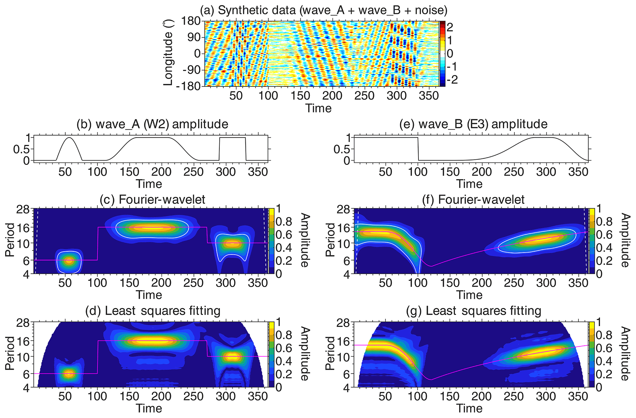
Figure 1 (a) Synthetic data containing wave_A (westward-propagating with zonal wavenumber 2 or W2) and wave_B (eastward-propagating with zonal wavenumber 3 or E3), along with noise. (b) Amplitude of wave_A. (c) Phase of wave_A (magenta line) and Fourier–wavelet amplitude spectrum for W2 (contour plot). The white curves indicate the 95 % confidence level, while the dashed white lines show the cone of influence. (d) Same as panel (c), except that the amplitude spectrum is derived with the least squares fitting method. (e–g) Same as panels (b–d) but for wave_B. The amplitude spectra are for E3.

The amplitude of wave_A is depicted in Fig. 1b. It changes between 0 and 1 over time in an arbitrary manner. The period of wave_A also changes over time, as shown in Fig. 1c. Also presented in Fig. 1c is the amplitude of W2, which is derived using the Fourier–wavelet method. The white curves indicate the 95 % significance level estimated, using the method described by Torrence and Compo (1998). The dashed white lines show the cone of influence, outside of which the edge effect may not be negligible. The Fourier–wavelet spectrum successfully identifies spectral peaks at the period of wave_A. The spectral amplitude tends to exceed the significance threshold when the amplitude of wave_A is above 0. Figure 1d is the same as Fig. 1c but is derived with the least squares fitting method, which is often used for studying global-scale waves in the MLT region (e.g., Fan et al., 2022; Qin et al., 2022b). The analysis was performed using time windows that are 3 times the wave period, which is a common choice in investigations of traveling planetary waves (e.g., Forbes and Zhang, 2015; Yamazaki and Matthias, 2019). The amplitude is not computed at the beginning and end of the data, where the length of the data is less than 3 times the wave period. There is good agreement between the results derived with the Fourier–wavelet (Fig. 1c) and least squares fitting (Fig. 1d) methods. However, the computation time for the Fourier–wavelet method is approximately $\frac{\mathrm{1}}{\mathrm{100}}$ that of the least squares fitting method, highlighting the advantage of the Fourier–wavelet method in terms of computation speed. Figure 1e–g correspond to Fig. 1b–d but for wave_B. Again, the Fourier–wavelet spectrum succeeds in identifying the amplitude and period of wave_B.

3.2 GAIA simulation: tides and traveling planetary waves during August–October 2019

There was an Antarctic sudden stratospheric warming in September 2019 (Lim et al., 2020; Rao et al., 2020; Yamazaki et al., 2020a). Although this event is categorized as a minor warming (i.e., no reversal of the zonal mean flow at 10 hPa), it was unusually strong for a Southern Hemisphere event in various measures (Lim et al., 2021), and its effects were observed at different layers of the atmosphere (e.g., Goncharenko et al., 2020; Noguchi et al., 2020; Safieddine et al., 2020; Wargan et al., 2020; Yamazaki et al., 2020a; Gan et al., 2023). A global simulation of the September 2019 sudden stratospheric warming event was presented by Miyoshi and Yamazaki (2020), based on the whole-atmosphere model GAIA. GAIA stands for the Ground-to-topside model of Atmosphere and Ionosphere for Aeronomy, and detailed model descriptions can be found in Jin et al. (2011) and Miyoshi et al. (2017). Figure 2a shows the polar stratospheric temperature and zonal mean zonal wind velocity at 60^∘ N at 10 hPa during August–October, as derived from the GAIA model. A rapid increase in the polar temperature in September and a concurrent reduction in the zonal mean zonal wind velocity are evident, which indicates the occurrence of the sudden stratospheric warming. Since the model is constrained by the JRA-55 reanalysis (Kobayashi et al., 2015) below a height of 40 km, these results strongly reflect the JRA-55 predictions.

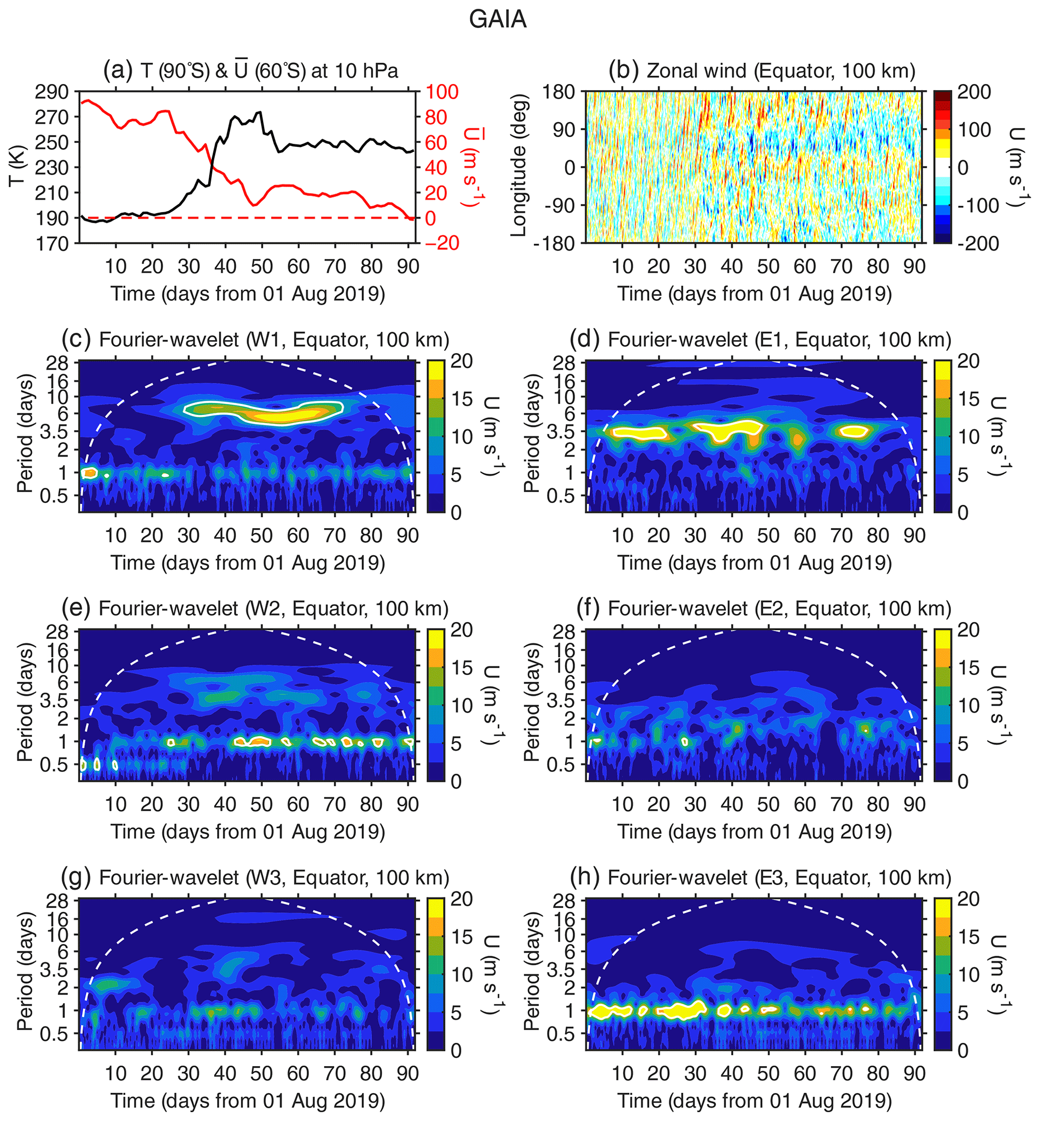
Figure 2 GAIA model simulation for the period August–October 2019. (a) Polar temperature and zonal mean zonal wind velocity at 60^∘ N at 10 hPa. (b) Zonal wind velocity over the Equator at a height of 100 km. (c–h) Fourier–wavelet spectra of the equatorial zonal wind velocity at 100 km for (c) the westward-propagating zonal wavenumber 1 (W1) component, (d) the eastward-propagating zonal wavenumber 1 (E1) component, (e) the westward-propagating zonal wavenumber 2 (W2) component, (f) the eastward-propagating zonal wavenumber 2 (E2) component, (g) the westward-propagating zonal wavenumber 3 (W3) component, and (h) the eastward-propagating zonal wavenumber 3 (E3) component. The white curves indicate the 95 % confidence level, while the dashed white lines show the cone of influence.

Figure 2b depicts hourly values of the zonal wind velocity over the Equator at an altitude of 100 km as a function of time and longitude. The zonal wind velocity shows considerable variability within the range of ±200 m s⁻¹, which is mostly due to waves generated in the region below 40 km. Figure 2c–h show Fourier–wavelet spectra of the equatorial zonal wind velocity at 100 km for different wave components.

In Fig. 2c, the amplitude of the W1 component at a period T of ∼ 6 d is enhanced around days 40–70. Earlier studies found that the amplitude of the Q6DW (W1; T∼6 d) during the September 2019 sudden stratospheric warming was unusually large compared to its seasonal climatology and had a significant impact on the ionosphere (Lin et al., 2020; Gu et al., 2021; Lee et al., 2021; Ma et al., 2022; Qin et al., 2021a; Yamazaki et al., 2020a; Miyoshi and Yamazaki, 2020; Mitra et al., 2022). In Fig. 2e, there is also a hint of the enhanced Q4DW (W2; T∼4 d) and Q7DW (W2; T∼7 d) around the same time.

In Fig. 2d, the UFKW (E1; T∼3.5 d) is seen throughout the period. In Fig. 2g, the Q2DW (W3; T∼2 d) is seen at the beginning of August 2019, but its amplitude is below the significance threshold. Their wave activity seems unrelated to the occurrence of the sudden stratospheric warming. Also, there is no apparent correlation between the sudden stratospheric warming and tidal activity. The most prominent tidal mode in these figures is DE3 (Fig. 2h). The amplitude of DE3 is known to be largest during August–October (e.g., Zhang et al., 2006; Akmaev et al., 2008; Yamazaki et al., 2023).

3.3 SD/WACCM-X simulation: tidal variability during January–February 2009

A major Arctic sudden stratospheric warming occurred in January 2009 (Manney et al., 2009; Harada et al., 2010). Whole-atmosphere simulations of this event were presented by several authors (e.g., Fuller-Rowell et al., 2011; Jin et al., 2012; Sassi et al., 2013; Pedatella et al., 2014; Siddiqui et al., 2021). Siddiqui et al. (2021) used the Whole Atmosphere Community Climate Model with thermosphere and ionosphere extension (WACCM-X) (Liu et al., 2018) with specified dynamics (SD), in which the region below 50 km is constrained by the Modern-Era Retrospective Analysis for Research and Applications, Version 2 (MERRA-2; Gelaro et al., 2017). The polar temperature and zonal mean zonal wind velocity at 60^∘ N at 10 hPa derived from this SD/WACCM-X simulation are plotted in Fig. 3a for the period of January–February 2009. The reversal of the zonal mean flow is seen on day 23, confirming that this event is a major warming.

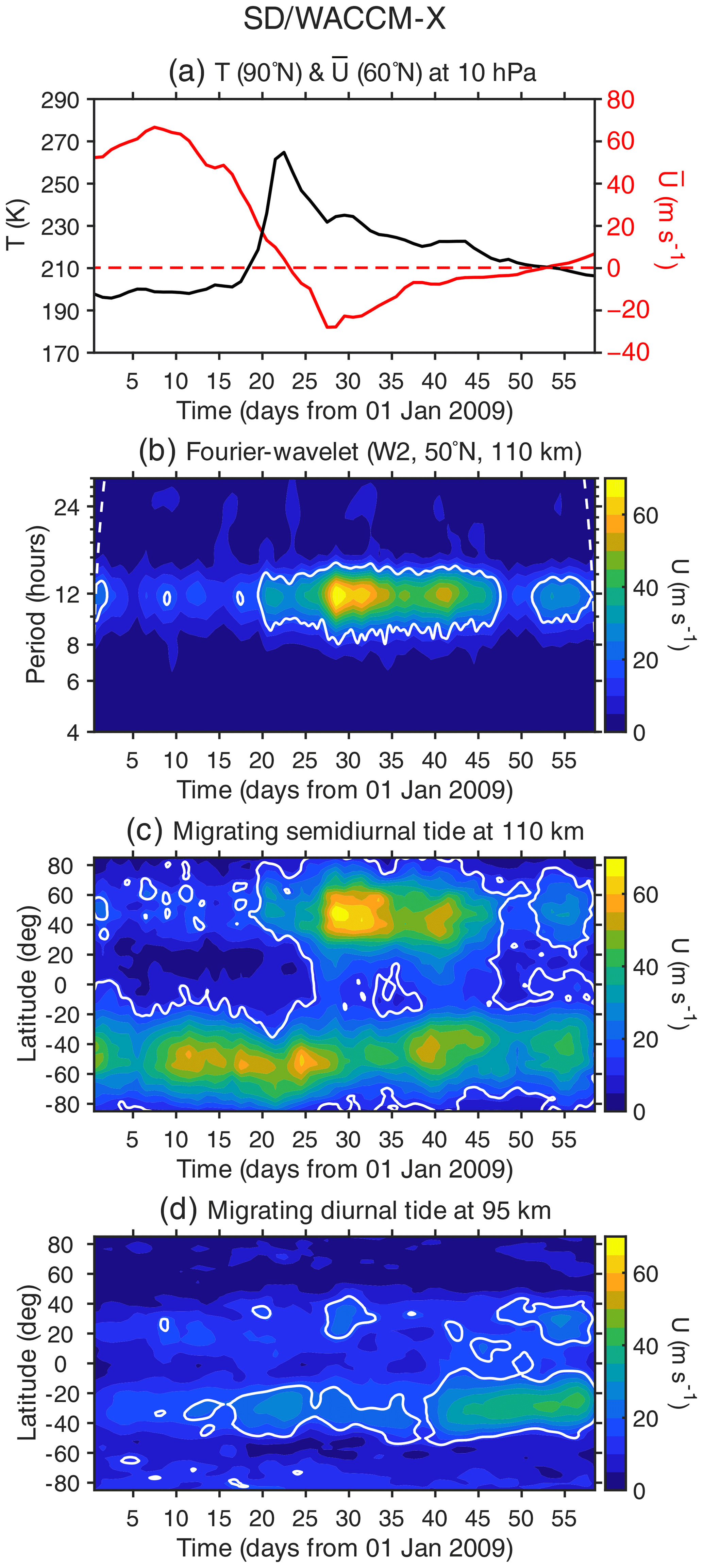
Figure 3 SD/WACCM-X model simulation for the period January–February 2009. (a) Polar temperature and zonal mean zonal wind velocity at 60^∘ N at 10 hPa. (b) Fourier–wavelet spectrum of the zonal wind velocity at 50^∘ N and 110 km. The white curves indicate the 95 % confidence level, while the dashed white lines show the cone of influence. (c) Amplitude of the migrating semidiurnal tide in the zonal wind velocity at 110 km, as determined by the Fourier–wavelet technique. (d) Amplitude of the migrating diurnal tide in the zonal wind velocity at 95 km, as determined by the Fourier–wavelet technique.

Observational studies have found large semidiurnal variations in the ionosphere during the January 2009 sudden stratospheric warming (Goncharenko et al., 2010a, b; Fejer et al., 2010; Yue et al., 2010). Numerical studies clarified that the semidiurnal ionospheric variations are due to the enhancement of semidiurnal tides that are generated in the lower atmosphere and propagate into the ionosphere (Jin et al., 2012; Wang et al., 2014; Pedatella et al., 2014). Figure 3b shows the W2 component of the Fourier–wavelet spectrum for the zonal wind velocity at 50^∘ N and 110 km. An enhancement of SW2 (W2; T=12 h) is clearly visible, following the reversal of the zonal mean flow. By performing the Fourier–wavelet analysis at different latitudes, it is possible to visualize the global structure of SW2 (Fig. 3c). It can be seen from Fig. 3c that the amplitude of SW2 increased and decreased in the Northern and Southern hemispheres, respectively, during the sudden stratospheric warming. A similar plot is shown in Fig. 3d but for DW1 (W1, T=24 h) and at 95 km, where the amplitude of DW1 is largest. The relationship between sudden stratospheric warmings and DW1 tidal variability was discussed in Siddiqui et al. (2022).

3.4 SD/WACCM-X simulation: traveling planetary waves during January–May 2016

A sudden stratospheric warming that coincides with the spring transition is called a final warning (e.g., Black and McDaniel, 2007; Matthias et al., 2021). Studies have noted that a final warming event is often accompanied by a strong Q10DW (W1; T∼10 d) in the MLT region (Yamazaki and Matthias, 2019; Yu et al., 2019; Yin et al., 2022; Qin et al., 2022b). Examples include the final warming event in March 2016. Figure 4a shows the polar temperature and zonal mean zonal wind velocity at 10 hPa, as obtained from the SD/WACCM-X simulation presented by Gasperini et al. (2020). The direction of the zonal mean flow reversed from eastward to westward on day 65 and did not turn eastward again until the next winter.

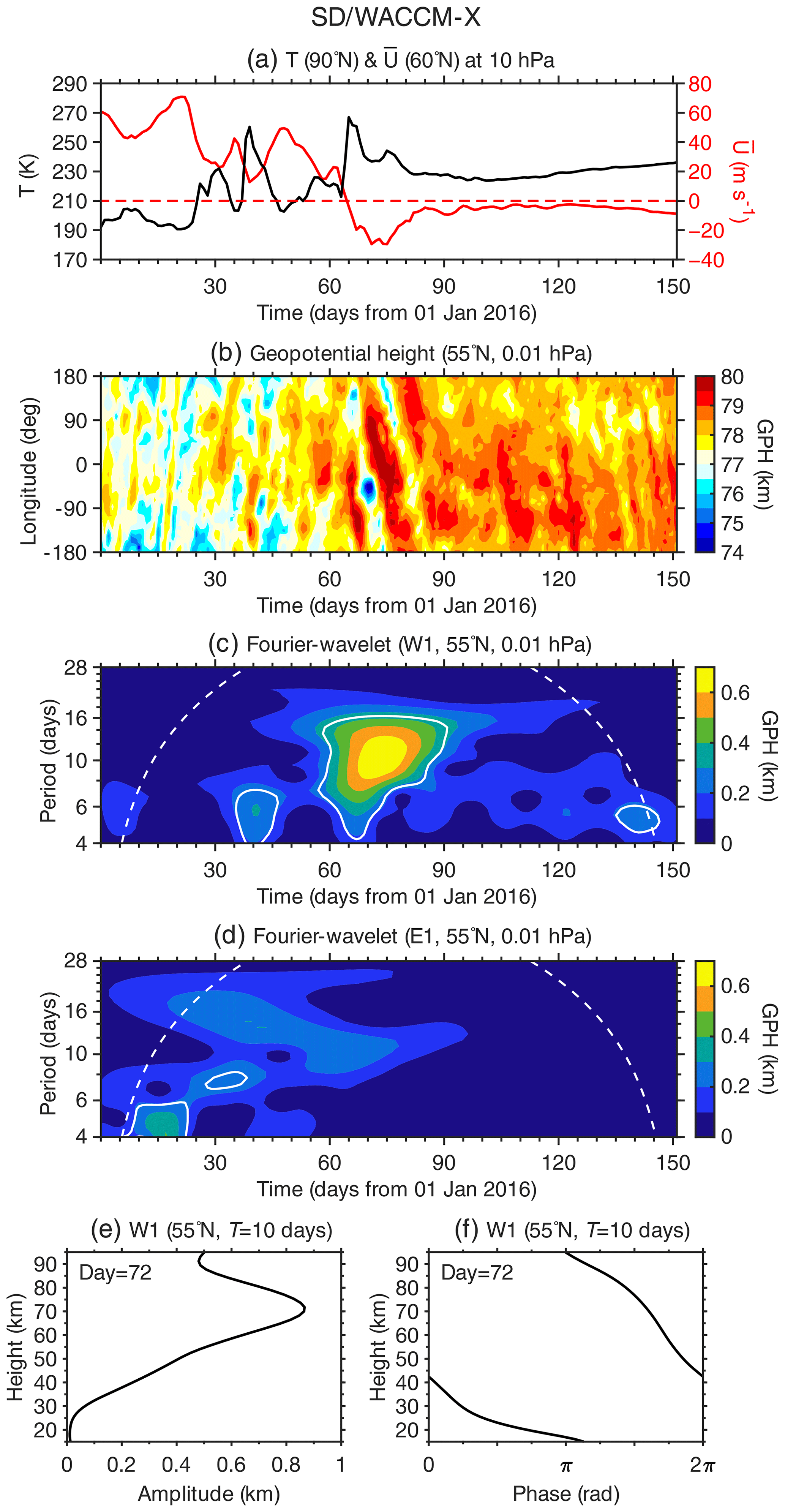
Figure 4 SD/WACCM-X model simulation for the period January–May 2016. (a) Polar temperature and zonal mean zonal wind velocity at 60^∘ N at 10 hPa. (b) Geopotential height at 55^∘ N at 0.01 hPa. (c–d) Fourier–wavelet spectra of the geopotential height at 55^∘ N at 0.01 hPa for (c) the westward-propagating zonal wavenumber 1 (W1) component and (d) the eastward-propagating zonal wavenumber 1 (E1) component. (e–f) Height profiles of the (e) amplitude and (f) phase of the W1 component at a period of 10 d at 55^∘ N and 0.01 hPa on day 72, as determined by the Fourier–wavelet technique.

Figure 4b displays daily values of the geopotential height at 0.01 hPa (∼ 77 km) as a function of time and longitude, where a westward-propagating wave-like perturbation is visible during the final warming. The W1 and E1 components of the Fourier–wavelet spectrum obtained from these data are presented in Fig. 4c and d, respectively. A burst of the Q10DW (W1; T∼10 d) during the final warming can be easily identified in the W1 spectrum (Fig. 4c). The height profiles of the amplitude and phase of the Q10DW are depicted in Fig. 4e and f, respectively, for day 72. The peak of the amplitude is seen at ∼ 70 km. The downward phase propagation (Fig. 4f) is consistent with the upward energy propagation of the Q10DW. The characteristics of the Q10DW during the March 2016 final warming derived with the Fourier–wavelet method are in good agreement with the observations presented by Yamazaki and Matthias (2019), based on the least squares fitting technique.

As a brief summary, the results presented in Sect. 3.2–3.4 demonstrate that global-scale wave spectra derived using the Fourier–wavelet method described in Sect. 2 are useful for identifying various types of tides and traveling planetary waves in the MLT region and their temporal variability. The structures of the global-scale waves can be determined by performing the Fourier–wavelet analysis at different latitudes and heights.

4 Conclusions and future directions

This study describes a simple method for deriving Fourier–wavelet spectra from 2-D longitude–time data. The method is conceptually similar to that of Hayashi (1971), which first performs the Fourier analysis in longitude and then performs the Fourier analysis in time. In the proposed technique, the Fourier analysis in time is replaced by the wavelet analysis (Torrence and Compo, 1998), which can resolve wave activity localized in time. Briefly, the implementation of the technique involves two steps. In the first step, the Fourier transform is performed in longitude, and then the time series of the sine and cosine Fourier coefficients are derived. In the second step, the wavelet transform is performed on these time series, and then real and imaginary wavelet coefficients are derived. Using these wavelet coefficients, Fourier–wavelet spectra can be obtained separately for eastward- and westward-propagating waves with different zonal wavenumbers (see Sect. 2 for details).

Easy-to-use software for computing Fourier–wavelet spectra is created in two user-friendly languages, i.e., MATLAB and Python, and made available at https://igit.iap-kborn.de/yamazaki/fourierwavelet (last acess: 18 August 2023). Application examples, based on this Fourier–wavelet software, are presented in Sect. 3. The results suggest that the technique can successfully identify tides and traveling planetary waves in the mesosphere and lower thermosphere (MLT) region and their transient response to sudden stratospheric warming events (Sect. 3.2–3.4). The Fourier–wavelet method has an advantage over other existing methods in that the computation is fast. In the example presented in Sect. 3.1, the computation time for the Fourier–wavelet method is approximately $\frac{\mathrm{1}}{\mathrm{100}}$ that of the least squares fitting method.

Future work includes the improvement of the technique for faster computation and broader applications. The technique introduced in this paper relies on the continuous wavelet transform. One criticism against the continuous wavelet transform is that it provides more information than what is actually available under Heisenberg's uncertainty principle (e.g., Yano and Jakubiak, 2016). Studies have shown that the discrete wavelet transform has some advantages, such as non-redundancy (and hence more efficient computation) and straightforward invertibility (e.g., Mallat, 1999; Yano et al., 2001b, a, 2004). The discrete wavelet transform may be implemented in the Fourier–wavelet technique.

An important limitation of the Fourier–wavelet technique is that it can resolve only global-scale waves. Along with tides and traveling planetary waves, gravity waves are also important in the MLT region (e.g., Fritts and Alexander, 2003; Smith, 2012), with a wide range of zonal wavenumbers (up to 100 or so; e.g., Miyoshi and Fujiwara, 2008; Liu et al., 2014). Since gravity waves are often localized in space, the Fourier–wavelet technique would not be able to fully capture them. A 2-D wavelet analysis (e.g., Kikuchi and Wang, 2010) would be useful. An easy-to-implement wavelet–wavelet technique for evaluating gravity–wave amplitudes and phases may be developed as an extension of the Fourier–wavelet technique presented in this paper.

Although this study has focused on waves in the MLT region, the Fourier–wavelet method could be applied to data from other regions of the atmosphere. The technique may also be useful in research areas outside of atmospheric science. The extent of applicability of the technique is still to be explored.