Climate model Selection by Independence, Performance, and Spread (ClimSIPS v1.0.1) for regional applications

As the number of models in Coupled Model Intercomparison Project (CMIP) archives increase from generation to generation, there is a pressing need for guidance on how to interpret and best use the abundance of newly available climate information. Users of the latest CMIP6 seeking to draw conclusions about model agreement must contend with an “ensemble of opportunity” containing similar models that appear under different names. Those who used the previous CMIP5 as a basis for downstream applications must filter through hundreds of new CMIP6 simulations to find several best suited to their region, season, and climate horizon of interest. Here we present methods to address both issues, model dependence and model subselection, to help users previously anchored in CMIP5 to navigate CMIP6 and multi-model ensembles in general. In Part I, we refine a definition of model dependence based on climate output, initially employed in Climate model Weighting by Independence and Performance (ClimWIP), to designate discrete model families within CMIP5 and CMIP6. We show that the increased presence of model families in CMIP6 bolsters the upper mode of the ensemble's bimodal effective equilibrium climate sensitivity (ECS) distribution. Accounting for the mismatch in representation between model families and individual model runs shifts the CMIP6 ECS median and 75th percentile down by 0.43 ^∘C, achieving better alignment with CMIP5's ECS distribution. In Part II, we present a new approach to model subselection based on cost function minimization, Climate model Selection by Independence, Performance, and Spread (ClimSIPS). ClimSIPS selects sets of CMIP models based on the relative importance a user ascribes to model independence (as defined in Part I), model performance, and ensemble spread in projected climate outcome. We demonstrate ClimSIPS by selecting sets of three to five models from CMIP6 for European applications, evaluating the performance from the agreement with the observed mean climate and the spread in outcome from the projected mid-century change in surface air temperature and precipitation. To accommodate different use cases, we explore two ways to represent models with multiple members in ClimSIPS, first, by ensemble mean and, second, by an individual ensemble member that maximizes mid-century change diversity within the CMIP overall. Because different combinations of models are selected by the cost function for different balances of independence, performance, and spread priority, we present all selected subsets in ternary contour “subselection triangles” and guide users with recommendations based on further qualitative selection standards. ClimSIPS represents a novel framework to select models in an informed, efficient, and transparent manner and addresses the growing need for guidance and simple tools, so those seeking climate services can navigate the increasingly complex CMIP landscape.

1 Introduction

Since its inception in 1995, the Coupled Model Intercomparison Project (CMIP) has guided the climate science community in a coordinated effort to understand how climate variability and change are represented by coupled ocean–atmosphere–cryosphere–land general circulation models (GCMs; Meehl et al., 1997, 2000; Taylor et al., 2012; Eyring et al., 2016). The backbone of international climate assessments (IPCC, 2021), the CMIP's common experiments have generated a range of possible future climate outcomes representative of a range of modeling strategies, socioeconomic decision-making, and inherent systemic internal climate variability. Generation to generation, CMIP model archives have grown, due to the participation of new modeling centers and to the recognition that multiple realizations of a single model provide valuable estimates of uncertainty arising from internal variability (e.g., Haughton et al., 2014; Deser et al., 2020; Maher et al., 2021a). Though these larger multi-model ensembles represent advancements in global coordination and uncertainty representation, they present interpretation and utilization challenges for downstream users (Dalelane et al., 2018).

1.1 The composition of the CMIP

Interpreting results derived from multiple CMIP models is complicated by the fact that the CMIP is an “ensemble of opportunity”; the project assembles all available climate projections that adhere to its simulation guidelines (Knutti et al., 2010). This inclusive strategy collects “best guesses” from modeling groups with the capacity to participate, which range from long-running, well-funded climate model development programs to brand-new groups with the computational resources to run a version of an existing climate model. While being inclusive, such ensembles of opportunity are not designed to be a representative sample of multi-model uncertainty in the way most would envision. For example, one might consider a representative sample of multi-model uncertainty to be a distribution put forth by a set of distinct climate models with different but plausible strategies for simulating the Earth system, equally represented by a single-model run. Further, each of those distinct models could be represented by several runs that start from slightly different states (initial-condition ensemble members) to reflect internal variability and by several runs that differ by parameter values (perturbed-physics ensemble members) to reflect parametric uncertainty (Parker, 2013), with the same number of runs for each model to maintain equal representation.

In reality, though, CMIP6 features over 60 uniquely named models (and counting), while its predecessor CMIP5 featured on the order of 40. Uniquely named models range in terms of representation within the ensemble, from a single-model run to several-member perturbed-physics ensembles to 50-member single-model initial-condition large ensembles. Modeling centers often contribute several versions of their base model under different names as well (Leduc et al., 2016); these variants differ by, for example, the spatial resolution of some model components or entire sub-models (see Brands et al., 2023), which may influence their simulated climate in ways that are difficult to anticipate. Adding further complexity, models actually fall over a spectrum that ranges from effective replicates to fully independent entities. Different models share historical predecessors (Masson and Knutti, 2011; Knutti et al., 2013), conceptual frameworks, and, in some cases, source code (Boé, 2018; Brands, 2022b; Brands et al., 2023). An active field of research has developed to identify and manage these “hidden dependencies” through weighting or subselection of the broader CMIP archives (e.g., Bishop and Abramowitz, 2013; Sanderson et al., 2015; Knutti et al., 2017; Brunner and Sippel, 2023), but open questions remain, particularly with regards to how best to determine dependence within multi-model ensembles (Abramowitz et al., 2019; Annan and Hargreaves, 2017).

Dependence is important to identify within multi-model ensembles because a common assumption is that when models converge to the same outcome, their consensus suggests certainty or robustness (Parker, 2011, 2013). Dependence undermines this assumption because robustness requires different modeling approaches to agree. Because the CMIP is not systematically designed to equally sample different modeling approaches, ensemble agreement could be coming from a diverse set of models or could simply be coming from the same (or similar) models supporting an outcome repeatedly (Pirtle et al., 2010). Redundant agreement reflects certainty in a particular model's outcome but does not mean that that model's outcome is necessarily correct, nor that we should be more confident in that outcome overall. Too many highly dependent entities within an ensemble clearly shift and/or narrow uncertainty estimates (Merrifield et al., 2020), so it is, therefore, crucial to systematically identify dependencies and evaluate how they affect distributional statistics before statements about robustness or uncertainty are made.

One method that has been developed to ward against over-confident multi-model climate uncertainty estimates is Climate model Weighting by Independence and Performance (ClimWIP; e.g., Knutti et al., 2017; Lorenz et al., 2018; Brunner et al., 2019, 2020b). ClimWIP uses model output variables to identify (1) potential issues that preclude a model from successfully simulating a realistic future climate response (performance) and (2) similarities that suggest a model is a duplicate or close relation of another in the ensemble (independence). Initial versions of ClimWIP based performance and independence definitions on the same set of predictors, which led to concerns about convergence to reality. The basic concern was that as models improved, their (valid) agreement towards an outcome would be interpreted as dependence and result in them being downweighted. To address this concern, separate sets of predictors were introduced to define performance and independence within ClimWIP to allow for a straightforward and universal definition of dependence in line with prior knowledge of model origin (Merrifield et al., 2020).

In addition to providing an operational definition of dependence that can be used to contextualize CMIP-derived results, ClimWIP has the advantage of being available for general open use (Sperna Weiland et al., 2021; Gründemann et al., 2022) as part of the Earth System Model Evaluation Tool (ESMValTool; Righi et al., 2020). In the first part of this study, we revisit and refine ClimWIP's definition of dependence using long-term, large-scale climatological “fingerprints” that enhance the spread between models and reduce internal variability. We show that distances between different climate models and versions of the same model or even between initial-condition members derived from climatological fingerprints delineate levels of dependence within the CMIP more precisely than distances based on previous predictor sets. This allows us to better illustrate how ensemble composition has changed from CMIP5 to CMIP6 in low-dimensional projected space. These intermember distances also reveal the presence of broader “model families” within the CMIP comprised of similar models from different institutions. In light of this, we determine a potential point of separation between models in families and the rest of CMIP5 and CMIP6 (henceforth CMIP5/6) and validate the resulting family designations using model metadata. Finally, to better understand how dependence may affect CMIP uncertainty estimates, we investigate how restricting representation to one “vote” per family constrains distributions of effective equilibrium climate sensitivity (ECS; Gregory et al., 2004).

Sections 2 through 4 comprise Part I of this study. Section 2 details the CMIP5/6 base ensembles used throughout. In Sect. 3, refinements made to ClimWIP's dependence strategy for the purpose of defining model families are described. Model family designations are put forward in Sect. 4 and subsequently employed to introduce a one-vote-per-family constraint on ECS in CMIP5/6.

1.2 The CMIP for downstream applications

Understanding dependencies within a multi-model CMIP ensemble is only the first step to designing an ensemble suitable for a downstream climate service application (Dalelane et al., 2018). For many applications, using the entirety of a modern CMIP archive is too computationally expensive. It has been widely assumed within the impact and regional modeling communities that a subset of several CMIP simulations will suffice for most tasks, provided the subset retains key characteristics of the larger ensemble that is selected from such as spread (e.g., Evans et al., 2013; McSweeney and Jones, 2016; Christensen and Kjellström, 2020; Kiesel et al., 2020).

The questions are then as follows: how should one select a representative subset from a multi-model ensemble for a specific task? How many simulations are necessary? Should those simulations come from independent models so that model agreement means something (Sanderson et al., 2015)? Should they come from models that are considered well suited in reproducing observed climate in a particular region or season to inspire fidelity in the projected outcomes (Ashfaq et al., 2022)? Should the subset prioritize having extreme cool–wet and hot–dry representatives, while also sampling possible climatic states in between (Qian et al., 2021)?

We posit that all three considerations, model individuality (henceforth “independence”), model suitability for a task (henceforth “performance”), and model outcome range (henceforth “spread”), should be taken into account when subselecting from the CMIP archive. Existing subselection methods are typically based on two of the three considerations and can be broadly grouped into performance-based or spread-based categories.

While subselection can be based on performance alone (Ashfaq et al., 2022), studies that evaluate performance-based subselection tend to do so in conjunction with independence (Evans et al., 2013; Sanderson et al., 2015; Herger et al., 2018; Di Virgilio et al., 2022; Palmer et al., 2023). Evans et al. (2013) succinctly demonstrated that for small subsets to reflect the spread of larger ensembles, it is more important to account for model independence (defined in the study following Bishop and Abramowitz, 2013) than for model performance. Selection by model performance is usually anticipated to reduce ensemble spread, which can also pose issues if there is an interest in reproducing the mean of the base ensemble. Herger et al. (2018) established that an ensemble selected based on a performance ranking was sometimes worse at reproducing the base ensemble mean than an ensemble selected at random. Using a comprehensive method to select diverse and skillful model subsets from CMIP5, Sanderson et al. (2015) found the multi-model ensemble to be a “rather heterogeneous, clustered distribution, with families of closely related models lying close together but with significant voids in-between model clusters” via empirical orthogonal function (EOF) analysis. CMIP5's interdependencies allowed for stages of subselection, first removing redundant simulations (without reducing the effective number of models), then removing poor-performing simulations to improve ensemble mean state representation. More recently, Di Virgilio et al. (2022) and Palmer et al. (2023) built on these CMIP5-era strategies to support CMIP6 model subselection for regional modeling exercises. In Di Virgilio et al. (2022), CMIP6 models, represented by an individual ensemble member, were first filtered by performance for Australian climate applications, with top- and mid-tier performers further evaluated for dependencies based on the methods of Bishop and Abramowitz (2013) and Herger et al. (2018). The study then went a step further to also assess climate change signal diversity to determine whether their high-performing, independent subset effectively sampled the range of Australian climatic changes in CMIP6. In Palmer et al. (2023), a process-based European performance assessment for CMIP6 is presented. The study, an extension of the work of McSweeney et al. (2015), also incorporates a second filter based on ClimWIP's dependence definition (Brunner et al., 2020b) and notably finds that regional model selection can differ from approaches targeting global metrics such as ECS that were central to CMIP5-era model subselection recommendations (CORDEX, 2018).

Spread-based subselection or selection, with the goal of maximizing climate change signal diversity, is often carried out either alone (e.g., Semenov and Stratonovich, 2015; McSweeney and Jones, 2016; Ruane and McDermid, 2017; Qian et al., 2021) or in conjunction with performance (Lutz et al., 2016) or independence (Mendlik and Gobiet, 2016). The clear application for this approach is impact studies where worst-case scenarios are often of interest. A common thread in spread-maximizing subselection studies is the concept of a “climate envelope”, typically defined by changes in spatiotemporal aggregations of surface air temperature (SAT) and precipitation (PR) fields. For example, Lutz et al. (2016) selected models from a base ensemble initially based on projected changes in SAT and PR means and then refined the selection using changes and historical performance of SAT and PR extreme indices. Similarly, the Representative Temperature and Precipitation GCM Subsetting (T&P) approach, developed by Ruane and McDermid (2017), sampled SAT and PR changes in terms of deviation from their respective ensemble medians. This allows for selected model combinations that span the cool–hot, wet–dry quadrants, as well as the “neutral” center, of the model ensemble. Qian et al. (2021) further advanced spread-maximizing subselection by evaluating the T&P approach against the Katsavounidis–Kuo–Zhang (KKZ) algorithm (Katsavounidis et al., 1994), in which members are recursively selected to best span the spread of an ensemble. While both approaches had merit, the KKZ approach was more likely than the T&P approach to perform better than a randomly selected five-GCM subset in terms of both error in relation to the full-ensemble mean and coverage of the full-ensemble spread.

Despite the numerous model subselection approaches available, the process remains somewhat burdensome to users and often requires several rounds of iterative filtering before a subset of a user's desired size is reached. And challenges can emerge depending on the choice of the starting filter: if performance is used as the starting filter, there is a risk the user is left with a set of very similar models that, though high-performing, are not independent and perhaps do not effectively sample ensemble spread. If spread is used as the starting filter, there is no way for a user to ensure that the models they select projecting the worst-case scenarios are realistic to begin with. If independence is used as a starting filter, which is not a common practice but perhaps should be, the user can be assured that model agreement is equivalent to robustness but may struggle to select the highest-performing or most unique projection from each model family.

To address these difficulties, we present an alternative approach to subselection that allows a user to simultaneously balance independence, performance, and spread interests and generate a subset of CMIP models of any size tailored to their specific application. The subselection method, Climate model Selection by Independence, Performance, and Spread (ClimSIPS; Merrifield and Könz, 2023), leverages a three-term cost function that grants the user freedom to decide how important independence, performance, and spread are (relative to one another) for the application. We demonstrate ClimSIPS for European climate applications in the second part of this study. First, the remaining methodological inputs are defined, including a performance score (also derived from ClimWIP) based on climatological biases that affect projections of European climate and a multivariate SAT and PR change spread metric. We then discuss the mechanics of subselection: the independence, performance, and spread cost function minimization and its visual representation, the subselection triangle. Because the cost function balances three interests, different combinations of models are selected as priorities shift. The subselection triangle, a ternary contour plot, summarizes which combination of models is optimal for each set of priorities.

ClimSIPS is demonstrated primarily within the CMIP6 ensemble for central European summer climate applications, beginning with a toy example. Upon extending the method to the full CMIP6 ensemble, we generate three-model subsets and formulate recommendations to help users navigate the subselection triangle. We compare ClimSIPS outcomes based on how a model is represented, whether by its ensemble mean (where applicable) or by an individual, spread-maximizing member. Finally, we generate five-model subsets for both central European summer climate and northern European winter climate applications. CMIP6 five-model subselection is highlighted in the main text, while CMIP5 five-model subselection is included in the Supplement.

Part II of this study is a case study of ClimSIPS for European climate applications, detailed in Sect. 5. Section 5.1 centers the definitions of performance and Sect. 5.2 the definitions of spread for European climate applications in the ClimSIPS protocol. The protocol is described in detail in Sect. 5.3, and the resulting three- and five-model subsets for each combination of independence, performance, and spread prioritization are presented in Sect. 5.4. To close, concluding remarks are made in Sect. 6.

2 CMIP models

We begin our assessment with ensembles comprised of all models (and all initial-condition and perturbed-physics ensemble members therein) with historical simulations and the highest emissions projection pathways: Shared Socioeconomic Pathway 5-8.5 (SSP5-8.5) for CMIP6 model projections (Eyring et al., 2016; O'Neill et al., 2016) and Representative Concentration Pathway 8.5 (RCP8.5) for CMIP5 model projections (Taylor et al., 2012). For inclusion in Part I, the models also must provide (1) an estimate of ECS, calculated from a 4×CO₂ run using the Gregory method (Gregory et al., 2004), and (2) the following monthly mean output fields (with their abbreviation and model output variable name given in brackets): near-surface 2 m air temperature (SAT; tas), precipitation (PR; pr), and sea-level pressure (SLP; psl). Further inclusion in Part II's European case studies requires the additional monthly mean output fields of sea surface temperature (SST; tos) and all-sky and clear-sky downwelling shortwave radiation at the surface (rsds and rsdscs, respectively). All fields are conservatively remapped onto a ${\mathrm{2.5}}^{\circ }\times {\mathrm{2.5}}^{\circ }$ latitude–longitude grid. At the time of writing, 218 CMIP6 and 75 CMIP5 simulations met the aforementioned criteria for Part I, and 197 CMIP6 and 68 CMIP5 simulations met the further criteria for Part II; additional CMIP6 simulations will be considered in subsequent publications as fields become available in the CMIP6 next-generation archive, a standardized repository used by researchers at ETH Zurich (Brunner et al., 2020a).

The inclusion requirements each serve a specific purpose in the study. Historical SAT, SLP, and PR fields are explored as a means to set degrees of model dependence within the CMIP ensembles. The degrees of model dependence are then used to constrain ECS values through subsetting. Remaining historical model output fields establish model performance, and SSP5-8.5–RCP8.5 projections establish mid-century climate change spread for Part II's European case studies.

Tables 1 and 2 provide a summary of the CMIP6 and CMIP5 models included in the study, respectively. We assign each uniquely named model (37 in CMIP6 and 29 in CMIP5) a numerical identifier (column 1) to be used throughout Part I. Model name and member count are also noted, with members labeled as initial- condition ensemble members (IC), perturbed-physics ensemble members (PP), or differently initialized ensemble members (DI) for multi-member ensembles. We provide additional information about members used in Tables S1–S3 in the Supplement, including full “ripf” identifiers for CMIP6 and “rip” identifiers for CMIP5. The IC designation corresponds to the “r” or realization index, the DI to the “i” or initialization index, and the PP to the “p” or physics index. The “f” or forcing index, unique to CMIP6, is shared by all members of each model.

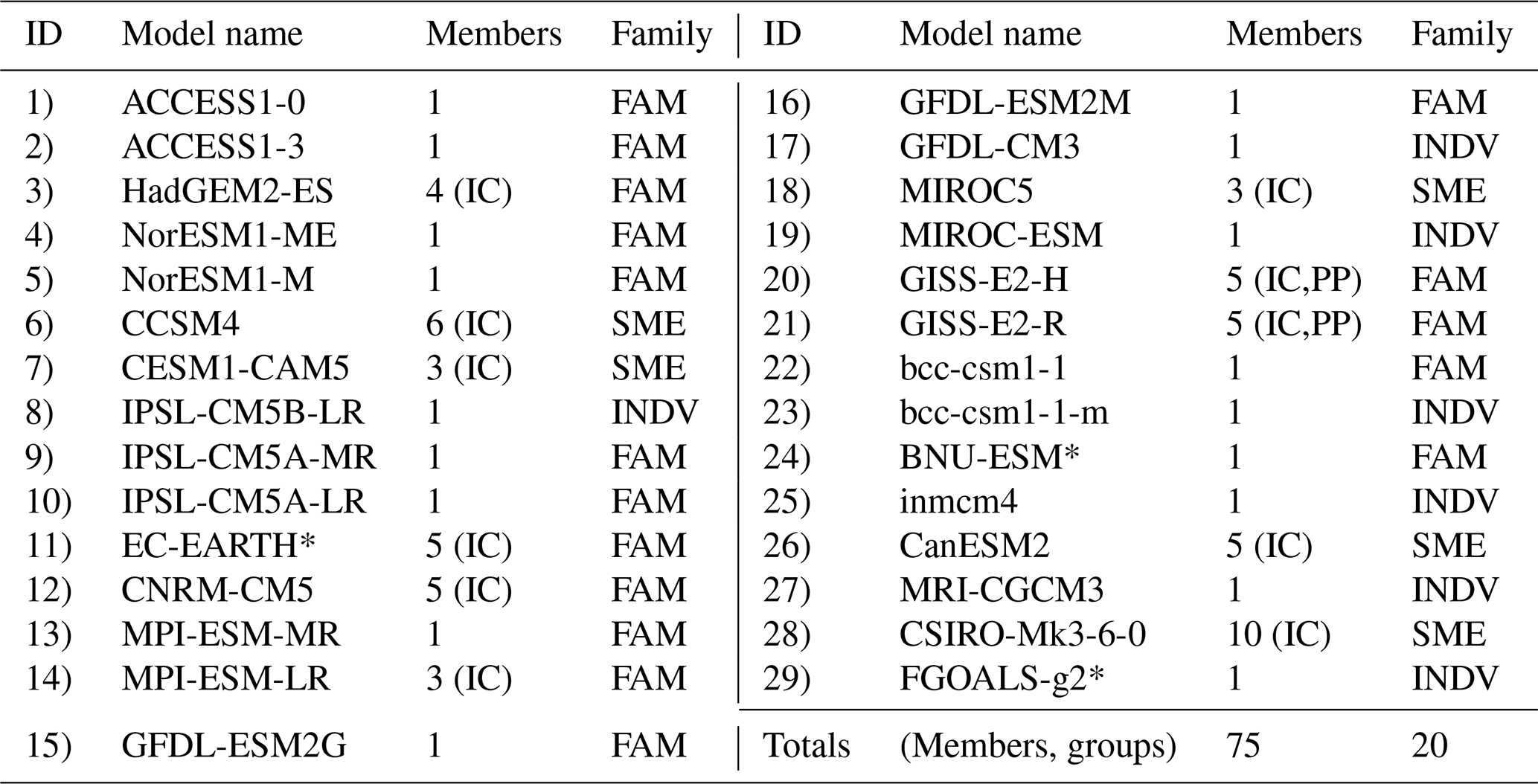
Finally, to familiarize the reader with the concept of model families we will subsequently define, we also list the family group status of each model. The designation, “INDV”, indicates a model is considered to be an individual represented by a single member. “SME” signifies that a model is a single-model ensemble or an individual represented by multiple members (e.g., initial-condition ensembles, perturbed-physics ensembles, combinations thereof). This means it was not found to be part of a broader multi-model family or “FAM” by the criteria we subsequently define. In total, the 218 CMIP6 simulations from 37 uniquely named models considered in Part I fall into 19 groups (seven multi-model families, eight single-model ensembles, and four individuals), and the 75 CMIP5 simulations from 29 uniquely named models fall into 20 groups (eight multi-model families, five single-model ensembles, and seven individuals). In Part II, 197 CMIP6 simulations from 34 uniquely named models and 68 CMIP5 simulations from 26 uniquely named models remain for the subselection exercise (Tables S1–S3).

Table 1 Summary of the CMIP6 multi-model ensemble. Starred models meet the inclusion criteria for Part I only at the time of writing.

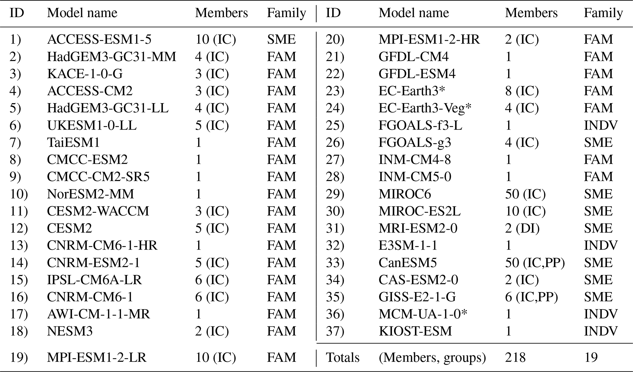
Table 2 Summary of the CMIP5 multi-model ensemble. Starred models meet the inclusion criteria for Part I only at the time of writing.

3 Revisiting model dependence

In prior studies, it has been shown that a climate model's origins and evolution can be traced via statistical properties of its outputs (e.g., Masson and Knutti, 2011; Bishop and Abramowitz, 2013; Knutti et al., 2013). Output-based model identification can uncover hidden dependencies within the ensemble, e.g., models that are similar because they share components or lineages but not names. The approach also has the advantage that it does not presume model similarity based on name alone; output from models in active development can evolve substantially from version to version (e.g., Kay et al., 2012; Boucher et al., 2020; Danabasoglu et al., 2020), while output from the same version of a model run at different modeling centers is often quite similar (Maher et al., 2021b). Risks arise, though, if model output used to determine similarity converges within a multi-model ensemble broadly and thus becomes ineffective at differentiating between dependent and independent models (Brands, 2022b). To reduce the risk of similar output conflating dependent and independent models, we update the model dependence strategy from the ClimWIP independence weighting scheme (Brunner et al., 2020b) to revisit the concept of model families within the CMIP.

ClimWIP defines model dependence using an intermember distance metric based on long-term, large-scale climatological averages (Merrifield et al., 2020). The rationale behind this underlying spatiotemporal aggregation is that it is able to identify an initial-condition or perturbed-physics ensemble as a single model (by averaging over differences due to internal variability or parameter uncertainty) while simultaneously maintaining varying degrees of differentiation between models in the ensemble overall. In practice, this balance between reducing intra-model or “within-model” intermember spread while still preserving inter-model or “between-model” intermember spread is key to a useful definition of dependence within the CMIP. It was found that the absolute values of global-scale annual average SAT and SLP climatologies are able to achieve this balance (Merrifield et al., 2020), but the extent of this has not yet been evaluated.

Here we explicitly investigate the within-model vs. between-model spread balance in ClimWIP's independence predictors to ensure they provide a suitable application-agnostic definition of model dependence for atmospheric studies. This is done by testing the sensitivity of the final root-mean-square error (RMSE) intermember distance metric to each methodological choice in ClimWIP, including temporal averaging period, spatial masking strategies, and predictor field choices. Intermember distance (I_ij) is calculated through pairwise RMSE between ensemble members i and j for each predictor field $\widehat{y}$ individually. Individual predictor RMSEs (ϕ_ij) are defined as

$$\begin{array}{}\text{(1)}& {\mathit{\varphi }}_{ij}=\sqrt{{\displaystyle \frac{{\sum }_{k=\mathrm{1}}^p{w}_k|{\widehat{y}}_i-{\widehat{y}}_j{|}^{\mathrm{2}}}{{\sum }_{k=\mathrm{1}}^p{w}_k}}},\end{array}$$

which reflects an RMSE weighted over the p grid points in a latitude–longitude domain, with w_k indicating the corresponding cosine latitude weights. Each ϕ_ij is normalized by its respective ensemble mean value ($\stackrel{\mathrm{‾}}{\mathit{\varphi }}$) and then averaged together to obtain a single I_ij for each member pair. As in Merrifield et al. (2020), I_ij is comprised of two individual predictor fields, global-scale annual average SAT and SLP climatologies:

$$\begin{array}{}\text{(2)}& I_{ij}={\displaystyle \frac{\mathrm{1}}{\mathrm{2}}}\sum _{l=\mathrm{1}}^{\mathrm{2}}{\left({\displaystyle \frac{{\mathit{\varphi }}_{ij}}{\stackrel{\mathrm{‾}}{\mathit{\varphi }}}}\right)}_l.\end{array}$$

To first order, I_ij is robust to methodological choices; the sensitivity testing did not reveal major shifts in whether a model was considered relatively dependent or independent with respect to the other models in the ensemble (See Figs. 1 and S1 in the Supplement). However, refining each methodological choice sharpens dependence delineations along the spectrum of dependence and lends further credence to the concept of model families.

The first methodological choice we revisit is the length of the climatological period of the global SAT and SLP predictors (Fig. 1). To reduce internal variability on decadal timescales, we extend the predictor climatological period from 1980–2014 (Brunner et al., 2020b) to 1905–2005, a common 101 years from the historical period of both CMIP5 and CMIP6. Illustrating the effect in the CMIP6 ensemble, we find reduced intermember distances between initial-condition ensemble members, highlighted in color, for the 1905–2005 averaging period (Fig. 1a) compared to the 1980–2014 period (Fig. 1b). The grouping effect of the longer predictor averaging period helps to further distinguish initial-condition and perturbed-physics ensemble members from members of other models (Fig. 1, light gray) in most cases. This differentiation is particularly clear in the case of CESM2-WACCM. The longer climatological averaging period distinguishes its three ensemble members from those of CESM2; with the shorter period, the two CESM2 model variants overlap (Fig. 1, models 11 and 12). In contrast, though, the longer averaging period fails to subdue internal variability enough to differentiate EC-Earth3-Veg from its base model, Earth3 (Fig. 1, models 23 and 24). The remaining internal variability in EC-Earth's global SAT and SLP fields is traceable to oscillations in the EC-Earth3 preindustrial control run from which both model variants are branched (Döscher et al., 2022). Functionally, this means that despite differing by coupled dynamic global vegetation, EC-Earth3 and EC-Earth3-Veg would be identified as one model by our independence metric. This ambiguity was also found in a model identification scheme that employs convolutional neural networks to daily output (Brunner and Sippel, 2023).

As the CMIP6 historical record spans 1850–2014 (Eyring et al., 2016) and the CMIP5 historical record spans 1870–2005 (Taylor et al., 2012), our choice of a 101-year averaging period could have been extended further back in time. However, we find that increasing the period back into the 19th century does not appreciably change intermember distances (not shown). Additionally, the 1905 start date may allow for backward compatibility of the metric with future generations of the CMIP should organizers decide to begin the historical period in the 20th century rather than the 19th century.

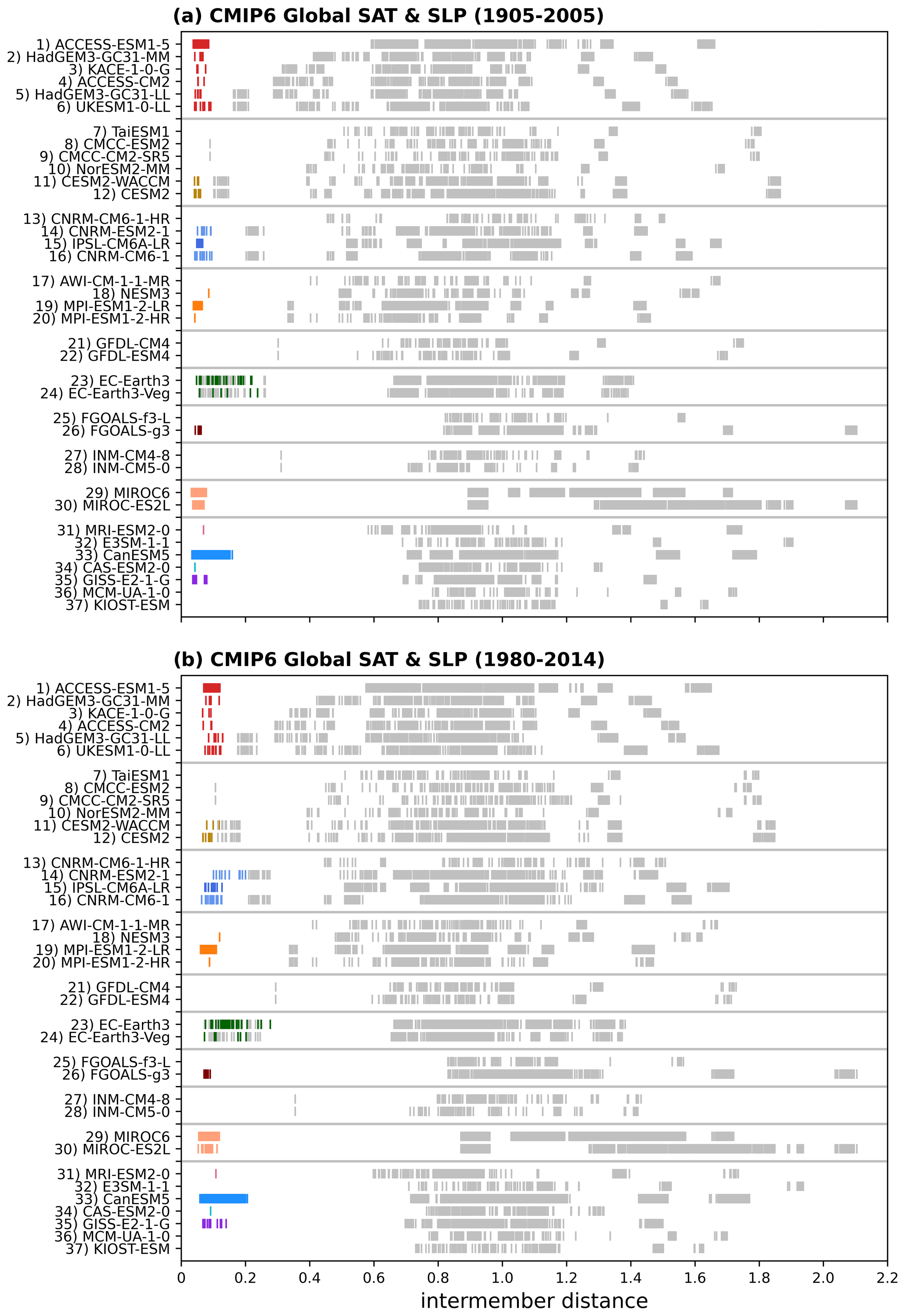
Figure 1 Intermember distances in CMIP6 based on Global SAT and SLP climatological fields averaged over the period (a) 1905–2005 and (b) 1980–2014. For each model, distances between initial-condition or perturbed-physics ensemble members are marked in color, and distances to members of the remaining models are marked in light gray.

The second methodological choice of interest is whether the dependence definition benefits from a spatial mask applied to the global SAT and SLP predictors. Spatial masking may not be a necessity; within-model spread can be reduced through temporal averaging, as seen in Fig. 1, and some level of between-model spread is provided by the choice to use predictor absolute values (Merrifield et al., 2020). Predictor absolute values provide between-model spread because it has not been a priority, historically, to calibrate or tune a model towards the absolute value of observed SAT or SLP (Mauritsen et al., 2012; Hourdin et al., 2017). The absolute magnitude of a climatic field tends to be seen as secondary to its relative change with respect to a historical base period for most applications (Jones and Harpham, 2013). The absolute value of global SAT in particular has been identified as an emergent property of climate models, reflecting differences underpinned by different model components and physical parameterizations (Schmidt, 2014). It is conceivable that in the future, however, the reduction of absolute global biases with respect to observations will become more of a priority to modeling centers, and the between-model spread we use to determine model diversity will disappear. Several emergent properties defined in the CMIP5 era have vanished in CMIP6, making this a credible concern (Simpson et al., 2021; Sanderson et al., 2021).

Spatial masking can help guard against independence predictor convergence because an atypically masked model output field is unlikely to feature in traditional model evaluation or tuning exercises. Further, spatial masks can be explicitly designed to leave behind “fingerprints” tailored to meet dependence objectives. Here we design a spatial fingerprint, shown in Fig. 2 for CMIP6 and Fig. S2 for CMIP5, that bolsters between-model spread and reduces within-model spread in the ClimWIP independence predictor fields. The SAT and SLP fingerprints, shown superimposed on their ensemble mean annual average climatologies (1905–2005) in Fig. 2e and f for CMIP6 and Fig. S2e and f for CMIP5, define model dependence for the remainder of the study.

The fingerprint design is conceptually simple; between-model spread is amplified by masking regions where it is low (Fig. 2, square hatching), and within-model spread is damped by masking regions where it is high (Fig. 2, diamond hatching). Though between-model spread is difficult to clearly define within the CMIP's multi-member, multi-model structure, it can be estimated via standard deviation across an ensemble comprised of one ensemble member per model. The first member is selected from each multi-member ensemble: r1i1p1 in CMIP5 and r1i1p1f1 where available in CMIP6, with exceptions listed in Table S4. Upon computing the standard deviation across the ensembles of one member per model, we mask out the region where between-model spread is at or below its 15th percentile (Fig. 2a,b, square hatching). This “low” between-model spread is largely confined to oceanic regions in the tropics and subtropics for both the SAT and SLP 1905–2005 climatologies.

In addition to regions of low between-model spread, we also select and mask regions of high (at or above the 85th percentile) within-model spread (Fig. 2c, d, diamond hatching). CMIP6 within-model spread is represented in Fig. 2c and d by the median of the standard deviations within the 12 CMIP6 initial-condition ensembles with five or more members (see Supplement Sect. S2). CMIP5 within-model spread is similarly defined within five initial-condition ensembles. Because the requirement of five or more members necessitates using a set of models to define internal variability rather than the full ensemble, we evaluate within-model spread within each individual model ensemble in Figs. S3 and S4 for SAT and SLP climatology, respectively. For SAT climatology, most models share regions of elevated internal variability across the Arctic and in particular, in the vicinity of the annual climatological sea ice edge in the Irminger and Barents seas (Fig. 2c; Davy and Outten, 2020). For SLP climatology (Fig. 2d), internal variability remains in parts of the Arctic and Antarctic, masking the Antarctic polar high region where between-model variability is also at a maximum (Fig. 2b). Patterns of elevated internal variability are broadly similar among the models evaluated (Figs. S3–S4), so we make the assumption that this within-model spread estimate is transferable to the other models in the ensemble that lack additional initial-condition ensemble members.

Results are not highly sensitive to precise percentile thresholds used to exclude regions of low between-model spread and high within-model spread; intermember distances are largely consistent for thresholds between the 5th and 20th percentile for between-model spread and the 80th and 95th percentile for within-model spread (Fig. S1). The 15th and 85th percentiles were chosen to limit the percentage of masked grid points to no more than 30 % of the domain total, similar in extent to a land mask. Masking the majority of the points in the domain increases the risk of relying on small-scale biases to define dependence, which complicates the interpretation of models being dependent because they are spatially similar overall. Masking very few points does not refine intermember distances much beyond those based on unmasked predictors (as used in Fig. 1), thus rendering the exercise unwarranted.

The third and final methodological choice we investigate is that of the fields in ClimWIP's independence predictor set. Due to the complexity and breadth of model output, innumerable combinations of different climatic fields can be put forth to define dependence. Because we aim for a dependence definition that is broadly applicable to studies of surface climate, we also considered PR as an addition to the independence predictor base set. However, we found that the inclusion of PR did not promote our primary goals: to group known dependencies and differentiate between models. The spatially masked annual-average PR climatology predictor, shown in Fig. S5, tended to reduce between-model differentiation within the ensemble as a whole, likely because the majority of its between-model spread is co-located and thus masked by high within-model spread in the tropical rain belts associated with the Intertropical Convergence Zone (ITCZ). For this reason, we chose to move forward with a dependence definition based solely on SAT and SLP fingerprints.

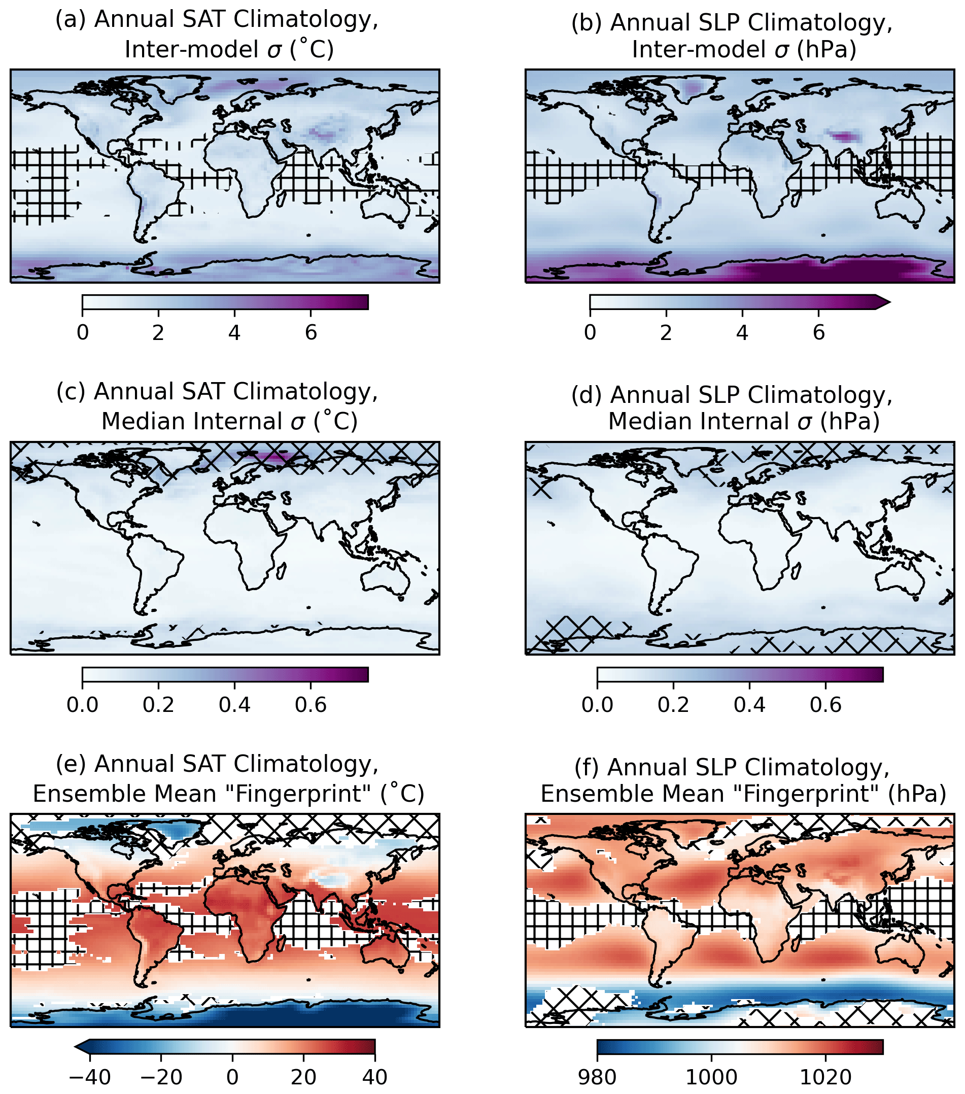
Figure 2 Determining the spatial “fingerprint” within the fields used to identify CMIP6 climate model dependence: annual mean SAT (^∘C) and SLP (hPa) climatology averaged over the period 1905–2005. (a, b) A measure of between-model spread of the dependence predictors computed as the standard deviation (σ) across a CMIP6 ensemble with only one member per model (see Table S4). Square hatching indicates where between-model spread is low, at or below its 15th percentile (calculated based on the spatial field). (c, d) Median internal variability of the dependence predictors computed as the median of the standard deviations within the 12 CMIP6 initial-condition ensembles with five or more members (ACCESS-ESM1-5, CanESM5, CESM2, CNRM-CM6-1, CNRM-ESM2-1, EC-Earth3, GISS-E2-1-G, IPSL-CM6A-LR, MIROC-ES2L, MIROC6, MPI-ESM1-2-LR, and UKESM1-0-LL). Diamond hatching indicates where median internal variability is high, at or above its 85th percentile. (e, f) Fingerprint used to determine dependence, shown as the ensemble mean climatology of the whole CMIP6 ensemble, with the regions of low between-model spread and high internal variability masked and hatched with square and diamond hatching, respectively.

4 Model families and their influence on CMIP uncertainty

Refining ClimWIP's dependence definition aids our effort to define model families within CMIP5/6. We pursue defining model families because many downstream applications, including ClimSIPS, benefit from a discrete definition of dependence rather than a continuous dependence spectrum. To achieve the discrete definition of dependence, each CMIP5/6 model is designated as either a single-model ensemble, part of a model family, or an individual (see Tables 1 and 2) based on intermember distances within the ensemble. We then make an effort to verify the designations through published model descriptions and reported metadata.

In Fig. 3, we show how intermember distances based on the sum of normalized RMSEs calculated from SAT and SLP fingerprints help to uncover model relationships within the CMIP. Intermember distances are presented for each model in one dimension (Fig. 3a, c) and, as recommended by Abramowitz et al. (2019), for the ensemble as a whole in a low-dimensional projected space (Fig. 3b, d). The second display strategy is appropriate because we find our matrix of I_ij meets the formal mathematical definition of a metric space. To be mathematically a metric, the distance from a model to itself must be zero, and distances between models must be positive, symmetric, and adherent to the triangle inequality, which states that the distance from A to B is less than or equal to the distance through an intermediary point C (Abramowitz et al., 2019). The low-dimensional projection is obtained through a standard metric multidimensional scaling (MDS) approach. The MDS method embeds the N-dimensional CMIP distance matrices into two-dimensional space while attempting to preserve relative positioning between models (Borg and Groenen, 2005). To assist the MDS method with model positioning, we ensure that ensemble members from each model are initially placed together and can thus settle into their final positions as a group. Without this initialization, there is a risk that an ensemble member may get stranded away from its group as the method contends with how best to map N dimensions to two dimensions.

In both one and two-dimensional visual representations, it is clear that the ensemble of opportunity has grown from CMIP5 (Fig. 3c, d) to CMIP6 (Fig. 3a, b); there are more uniquely named models in CMIP6 than in CMIP5 and, on average, more ensemble members per model. In projected space (Fig. 3b, d), models with multiple ensemble members are highlighted using a radius of similarity (shaded circles), a construct also conceived by Abramowitz et al. (2019). Here we employ this construct largely as a visual aid and set the radius to 2.5 times the maximum deviation of an individual ensemble member from its ensemble mean. Models are labeled by number in the projections, with numbers listed in Tables 1 and 2 and on the y axis of Fig. 3a and c.

In CMIP6, an ensemble “core” comprised of all but two models has emerged; the intermember distance metric identifies MIROC6 and MIROC-ES2L as considerably more independent from the rest of the ensemble (Fig. 3b). We use a broken axis in CMIP6's low-dimensional space projection to accommodate the two MIROC outliers and emphasize the structure of the CMIP6 core. In contrast, CMIP5 does not have the same level of core and outlier structure, and intermember distances create a more distributed dependence spectrum (Fig. 3d) similar to the one described in Sanderson et al. (2015).

In the one-dimensional representation, distances between a model's ensemble members are shown in color, distances to family members are shown in dark gray, and distances to the rest of the ensemble are shown in light gray (Fig. 3a, c). Beginning with the most dependent entities in the CMIP, the SAT and SLP fingerprint metric clusters initial-condition ensemble members at distances of around 0.05 in all but one case. The exception, EC-Earth3 and EC-Earth3-Veg (Fig. 3a, dark green, 23 and 24), exhibits overlapping intermember distances from 0.08 to 0.20, as stated previously, due to remaining decadal variability in the predictors (Döscher et al., 2022). At the next level of dependence, the intermember distance metric introduces a measure of disambiguation between initial-condition and perturbed-physics ensemble members, as illustrated by two models in CMIP6, CanESM5 (Fig. 3a, bright blue, 33) and GISS-E2-1-G (Fig. 3a, bright purple, 35). Strikingly, in Fig. 3b, CanESM5's two 25-member initial-condition ensembles can be seen clearly as two distinct clusters in two-dimensional space. CanESM5 initial-condition ensembles are reported to differ by wind stress remapping; conservative remapping is used for “p1” members, and bilinear regridding is used for “p2” members (Swart et al., 2019).

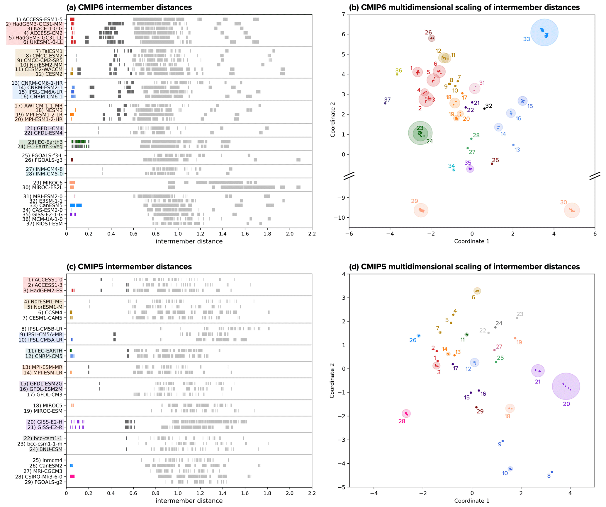
Figure 3 Intermember distances used to identify degrees of dependence within (a) CMIP6 and (c) CMIP5. For each model, within-model distances (i.e., initial-condition ensemble members or perturbed-physics ensemble members) are marked in color, distances to members of other similar models are marked in dark gray, and distances to members of the remaining models are marked in light gray. Models grouped into families are highlighted on the y axis. To better visualize levels of similarity within the multi-model ensembles, CMIP6 (b) and CMIP5 (d) intermember distances are projected from high-dimensional space into two dimensions using multidimensional scaling. Models are colored and labeled numerically as indicated in panels (a) and (c). Initial-condition and perturbed-physics ensembles are given a radius of similarity (shaded circles) equivalent to 2.5 times the maximum deviation from their ensemble mean. Note that in panel (b), a broken axis is used to emphasize the structure of the primary CMIP6 model core with respect to the independent constituents, MIROC6 and MIROC-ESL.

Continuing along the spectrum of dependence from most dependent to most independent, intermember distances reveal model similarities that would require high-level knowledge of CMIP model origins to determine a priori (Fig. 3a, c, dark gray). In this regime, where models are separated by distances of around 0.1 to 0.6, subjective decisions must be made regarding whether or not a model is part of a family. We chose two criteria to determine if a family should be formed: (1) a model family must be a self-contained group, i.e., all family members must be closer to each other than to other models, and (2) models within the family must have a median intermember distance to the rest of the family that is less than 0.56. This median intermember distance threshold was based specifically on the composition of CMIP6 to ensure that we did not simply define one large family within the ensemble's core (Fig. 3b). However, because it is ultimately a subjective threshold, we pursued further justification of model families in the literature.

To ensure that similar models form self-contained groups, we match intermember distances between pairs of models in one-dimensional space. For example, CMIP6's INM-CM4-8 and INM-CM5-0 are separated by a distance of 0.32 from each other as indicated by a dark-gray line in their respective rows in Fig. 3a. To assist with model pair matching, we ordered and used mutual colors for models that we anticipated would be similar enough to be grouped into families. In general, we predicted that models contributed by the same modeling center might be family members and then set about to determine if the assumption was substantiated by intermember distances. We also anticipated three “extended” families based on an analysis of model metadata, summarized in Tables S1–S3, and the work of Brands (2022b), which grouped models via shared atmospheric circulation error patterns. The first, shown in dark red (CMIP6 models 1–6, CMIP5 models 1–3) in Fig. 3, is comprised of models with UK Met Office Hadley Centre atmospheric components. In CMIP6, intermember distances show five of the six models highlighted in red on the y axis of Fig. 3a, satisfying both the self-contained group and median intermember distance threshold criteria to form a family. This grouping makes sense as all five models (HadGEM3-GC31-MM, KACE-1-0-G, ACCESS-CM2, HadGEM3-GC31-LL, and UKESM1-0-LL) use the same MetUM-HadGEM3-GA7.1 atmospheric component (Table S1). The sixth model, ACCESS-ESM1-5, does not satisfy the self-contained criteria and is closer to other models in CMIP6 than it is to its anticipated family members. This likely occurs because ACCESS-ESM1-5 uses a CMIP5-era HadGAM2 atmospheric component rather than the CMIP6-era MetUM-HadGEM3-GA7.1 atmospheric component, highlighting the potential for models in the same development stream to differentiate themselves from their successors. In CMIP5, a similar family of models with UK Met Office Hadley Centre atmospheric components is present (Fig. 3c, dark red, models 1–3), where it is comprised of three uniquely named models, ACCESS1-0, ACCESS1-3, and HadGEM2-ES. ACCESS1-0 and HadGEM2-ES also share HadGAM2 atmospheres, while ACCESS1-3 features a modified version of the UK Met Office Global Atmosphere 1.0 AGCM (UM7.3/GA1; Bi et al., 2012; Brands, 2022a). ACCESS1-3 is closer to ACCESS1-0 and HadGEM2-ES than to other CMIP5 models and thus joins the family group despite the differing atmospheric component, demonstrating that a family designation is more complex than just a single shared model component.

The second anticipated extended family, shown in goldenrod (CMIP6 models 7–12, CMIP5 models 4–7), features models with atmospheres that share commonalities with the National Center for Atmospheric Research (NCAR) Community Atmosphere Model (CAM). In CMIP6, there is a gap in pairwise intermember distance between models with a CAM5.3 atmosphere (CMCC-ESM2, CMCC-CM2-SR5) and models with a CAM6 atmosphere (CESM2 and CESM2-WAACM). Two additional models, TaiESM1 and NorESM2-MM, are similar enough to also be included in the family (Fig. 3a, goldenrod highlight), likely because their atmospheres are based on CAM5.3 and CAM6, respectively, with several alternative parameterizations incorporated (Lee et al., 2020; Seland et al., 2020). Though NorESM2-MM is closer to the CAM6-based models than the CAM5.3-based models in terms of intermember distance, it does end up placed towards the CAM5.3-based cluster in low-dimensional space due to how the MDS method chooses to optimize relative positioning (Fig. 3b). In CMIP5, there is less similarity seen between members of the CAM-based anticipated extended family (Fig. 3c, goldenrod, models 4–7), particularly between CESM1-CAM5 and the models based on CAM4, its predecessor atmospheric component (see Table S3). The four models (NorESM1-ME, NorESM1-M, CCSM4, and CESM1-CAM5) reside in the same region of low-dimensional space, but do not form a discernible cluster (Fig. 3d) and do not satisfy either criteria to be considered one extended family. Instead, NorESM1-ME and NorESM1-M form a family (Fig. 3c goldenrod highlight), while CCSM4 and CESM1-CAM5 remain as single-model ensembles.

The third anticipated extended family, shown in orange (CMIP6 models 17–20, CMIP5 models 13–14), is made of models that utilize ECHAM6 atmospheric components developed at the Max Planck Institute for Meteorology. In CMIP6, a gap is present between within- (Fig. 3a color) and between-model distances (Fig. 3a dark gray) in the grouping, which may be traceable to differences in horizontal resolution (Table S1). This anticipated family has also grown from CMIP5, which featured two ECHAM6.1-based model variants that differ by vertical atmospheric resolution and horizontal ocean resolution (Giorgetta et al., 2013), to CMIP6, which features four ECHAM6.3-based models contributed by different modeling centers. The family is positioned in a cluster towards the center of both CMIP ensembles in low-dimensional space (Fig. 3b, d).

In addition to the three anticipated families, several other families emerge upon assessing intermember distances. In CMIP5, the EC-EARTH and CNRM-CM5 initial-condition ensembles share a level of similarity on par with the other families, as do bcc-csm1-1 and BNU-ESM (Fig. 3c). In CMIP6, we find the three CNRM models to be similar enough to IPSL-CM6A-LR to satisfy the family criteria (Fig. 3a light blue and medium blue, models 13–16). Similarity in these cases cannot be traced to a particular atmospheric component model, but for CNRM and IPSL, similarity could have arisen through an effort to foster collaboration between the two French modeling groups after CMIP5 (Mignot and Bony, 2013) or due to similar ocean component models (Brands et al., 2023). The remainder of model families in both CMIP5 and CMIP6 feature models originating from the same modeling center. However, not all same center models are similar enough, in terms of intermember distance, to be considered potential relatives. For example, GFDL-CM3 is more similar to other CMIP5 models than it is to Earth system models from the same modeling group, GFDL-ESM2M and GFDL-ESM2G (Fig. 3d). In this case, a different atmospheric component model version accompanies the dissimilarity in historical model output; GFDL-CM3 uses a later-generation atmospheric component than GFDL-ESM2M and GFDL-ESM2G (See Table S3). Meanwhile, GFDL-ESM2M and GFDL-ESM2G only differ from each other by ocean component (Dunne et al., 2012) and do satisfy the criteria to form a family. CMIP6's FGOALS-f3-L and FGOALS-g3 are also found to be relatively distinct from each other in terms of intermember distance; the two models differ in atmospheric component, notably by the atmospheric finite differencing method (Zheng et al., 2020). The only models to share an atmospheric component and not form a family are CMIP6's MIROC6 and MIROC-ES2L. Though the two MIROC variants form a self-contained group, they are more distinct from each other in terms of intermember distance than most models pairs considered to be independent within the CMIP6 core and are thus considered independent single-model ensembles instead of a family.

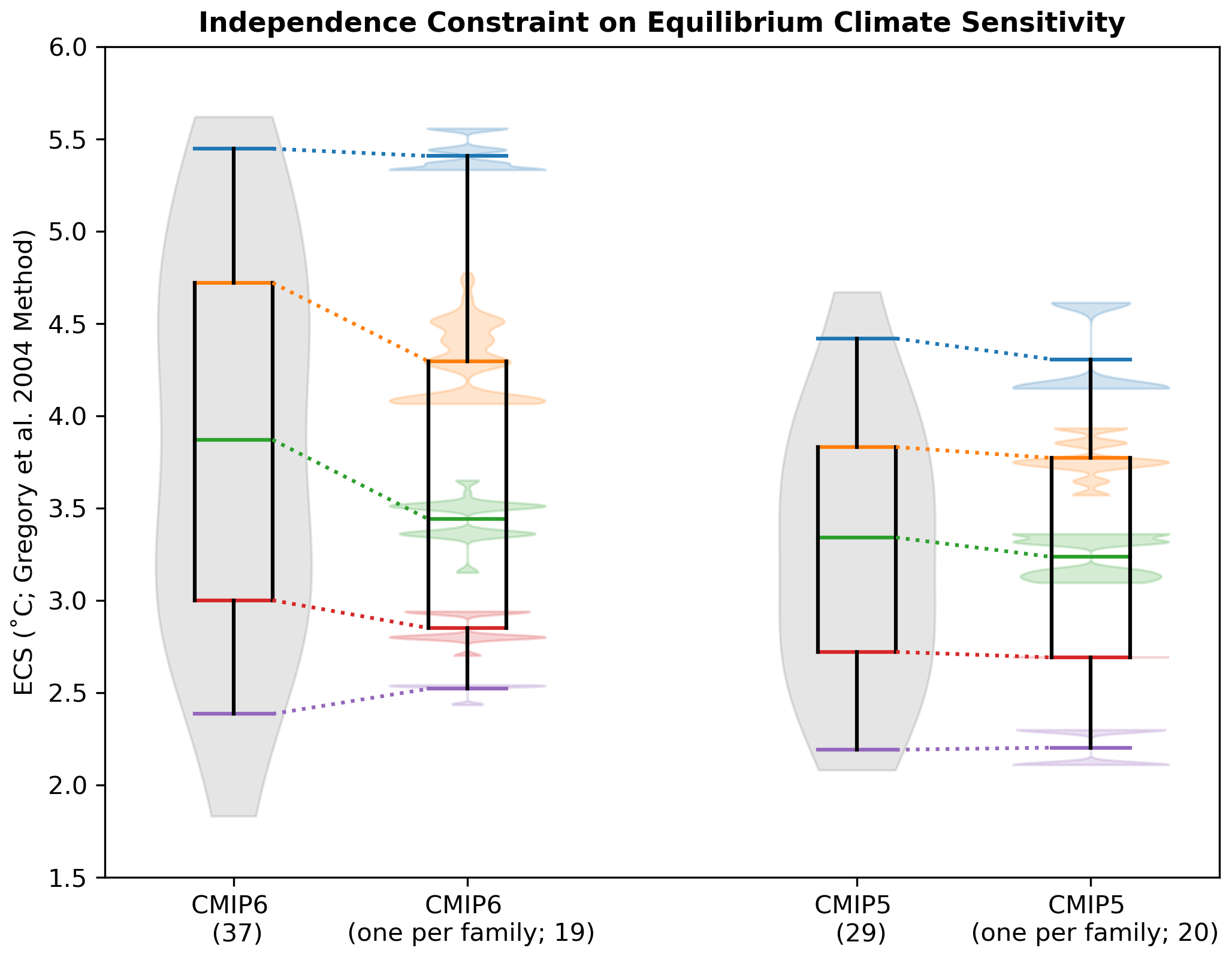
Figure 4 Comparison between the full distribution and the one-per-family subset distribution of effective equilibrium climate sensitivity (ECS) in CMIP6 and CMIP5. Full distributions are shown as a violin plot (gray), with the median (green) and the 5th (purple), 25th (red), 75th (orange), and 95th (blue) percentiles superimposed. One-per-family subset distributions of each percentile (violins) reflect 10 000 subsets from a bootstrap random selection of one model from each model family (see Fig. 3). The means of each percentile distribution are used to create the one-per-family box and whisker. The number of members in each distribution are given in parentheses.

One of the primary reasons we define model families is to enhance our understanding of how dependence influences CMIP uncertainty estimates. Model families establish a stricter definition of independence within the CMIP than the “one model, one vote” standard typically employed in multi-model assessments if weights (fractional votes) are not desired or possible (Knutti, 2010). The one model, one vote standard treats all uniquely named models in the ensemble as independent and allows them each to be represented by one simulation. By this standard, CMIP6 is represented by 37 independent entities, and CMIP5 is represented by 29 independent entities. We compare this traditional approach against a “one family, one vote” standard, where each model family, single-model ensemble, and individual is represented by one simulation. This reduces CMIP6's representation to 19 and CMIP5's to 20 independent entities.

We assess the impact of the one family, one vote independence constraint on distributions of ECS, a key climate metric reflecting the magnitude of warming a model projects in response to CO₂ doubling from preindustrial levels (Charney et al., 1979). We source ECS values primarily from the IPCC (Smith et al., 2021) and, when not available, from studies reporting to compute ECS via the Gregory et al. (2004) method. Further information on the sourcing of ECS is provided in the Supplement; the ECS values used are shown in Fig. S6. Raw distributions of ECS in CMIP5/6 are represented in Fig. 4 by both violin (gray shading) and box-and-whisker elements. The violin representation gives a sense of how the shape of the ECS distribution has evolved from CMIP5 to CMIP6, with CMIP6 having a more bimodal structure, a lighter low-ECS tail, and a heavier high-ECS tail than CMIP5. This is consistent with the highly publicized finding that a subset of CMIP6 models are “running hotter” than their CMIP5 predecessors (e.g., Flynn and Mauritsen, 2020; Zelinka et al., 2020; Tokarska et al., 2020); there are only five models with an ECS above 4 ^∘C in the CMIP5 distribution compared to 17 in the CMIP6 distribution. Box-and-whisker elements, superimposed on the violins, provide a way to investigate how different percentiles of the distribution compare between CMIP generations and shift under the new one family, one vote independence constraint. We focus on the 5th (purple), 25th (red), median (green), 75th (orange), and 95th (blue) percentiles. All percentiles have increased between CMIP5 and CMIP6, ranging from the 5th, which increases by 0.19 ^∘C (2.19 to 2.38 ^∘C), to the 95th, which increases by 1.03 ^∘C (4.41 to 5.45 ^∘C). Also notable is that no CMIP5 model has an ECS that exceeds CMIP6's 75th percentile of 4.72 ^∘C (see Fig. S6).

To ascertain if model dependence can explain the shift in ECS between CMIP generations, we apply the one family, one vote independence constraint to ECS in both ensembles via a bootstrap protocol. First, base ensembles are formed from the models (single-model ensembles and individuals) already represented by one ECS value. Subsequently, one member of each model family is randomly selected, and its ECS value joins the base ensemble to form a one-per-family ensemble. Percentiles are then computed, and the procedure is repeated 10 000 times to generate distributions of percentiles (Fig. 4 color-coordinated violin elements). Percentile distributions reflect the fact that model families span a range of ECS values, and the one-per-family distribution shifts depending on the combination of models selected. Finally, the overall one-per-family ensemble box-and-whisker element is constructed from the means of each percentile distribution.

In CMIP6, there are seven families, comprised of two to six models, to randomly select from (Fig. 3a label highlights). After 10 000 rounds of selection, the average CMIP6 one-per-family distribution (Fig. 4 second element from left) has reduced skewness towards high ECS compared to the raw CMIP6 distribution. The removal of dependent entities does not affect CMIP6's 95th percentile (Fig. 4 blue; 5.4 ^∘C) due to the certainty that at least 2 of the 19 models in the one-per-family distribution have an ECS above 5 ^∘C (E3SM-1-1 and CanESM5; Fig. S6). In contrast, the interquartile range (Fig. 4 red to orange) of CMIP6's one-per-family distribution is shifted toward lower values of ECS with respect to the raw distribution, to 2.85–4.29 ^∘C from 3.0–4.72 ^∘C. CMIP6 median ECS also shifts down by 0.43 to 3.44 ^∘C when representation is limited to one family, one vote. This suggests that the higher ECS mode of CMIP6's bimodal distribution is due, in part, to there being more “copies” of higher ECS models in the ensemble. Removing redundancies also constrains the lower tail of the distribution (Fig. 4 purple), which is set in the raw ensemble by the two models with ECS below 2 ^∘C, family members INM-CM4-8 and INM-CM5-0.

In CMIP5, of eight families, seven are comprised of two models, and one is comprised of three models (Fig. 3c label highlights). Selecting from CMIP5's smaller families (compared to CMIP6) results in a CMIP5 one-per-family distribution that is nearly identical to the raw CMIP5 distribution (Fig. 4 right). Limiting family representation does have a marginal impact on the CMIP5 95th percentile and median, shifting them each down by 0.11 ^∘C, but does not skew the distribution nor narrow its interquartile range as it does in CMIP6. This suggests the approach taken in IPCC AR5 where model dependence was not explicitly considered was reasonable. While dependencies exist in CMIP5, they happen to be distributed in a way that the mean and overall model spread is not strongly affected. We find that dependence alone cannot account for the full distributional shift in ECS between CMIP5 and CMIP6 but does reconcile the two somewhat, reducing the difference for CMIP6 and CMIP5 median ECS by over 60 %.

Ultimately, constraining by independence emphasizes that though there are significantly more simulations in CMIP6 than in CMIP5 (here 218 versus 75), there are not significantly more independent models in CMIP6 as of yet. Highly similar models appear more frequently in CMIP6 under different names, and increased representation has just happened to occur more for model families on the high end of the ECS distribution. It is important to note that limiting representation in this instance is not a comment on model quality in any way; it is only a comment on whether a model's historical output is sufficiently independent of other models in the ensemble. Because of the influence redundancies have on multi-model uncertainty distributions, model families are crucial for users to be aware of, whether or not they choose to sub-sample CMIP6.

5 ClimSIPS for European climate applications

For use in cases that require a subset of CMIP models, model dependence is one of three common ensemble design considerations. Equally important to subselection are model performance and spread between model outcomes in the chosen set. Discussed in the following subsections, we define performance with respect to observations over different periods of the historical record. Spread is calculated from projected regional changes between present climate, averaged from 1995–2014, and mid-century climate, averaged from 2041–2060 in CMIP6's SSP5-8.5 or CMIP5's RCP8.5 emissions scenario. Performance and spread definitions were designed to select sets of models to underpin European regional climate modeling efforts and impact assessments.

5.1 Performance metric

Performance centers on properties of a model that make it suited to simulating future European climatic states, as defined by a multivariate model–observation comparison metric. We aim to identify models with historical biases that would preclude them from accurately projecting future European climate rather than attempting to elevate one model over another based on its success in simulating a limited set of historical European climate variables. We focus on historical biases because all CMIP models have strengths and weaknesses in simulating aspects of the climate system, and it is not always clear that model's historical strengths will translate into future skill (Weigel et al., 2010). Historical biases, in contrast, highlight cases where models lack important dynamic or thermodynamic processes (Knutti et al., 2017) or are simply too hot, cold, wet, or dry to transition into a realistic future temperature or precipitation regime (Eyring et al., 2019).

Specifically, we compare all CMIP members with observations using ClimWIP's performance weighting strategy (Brunner et al., 2020b). We utilize predictor fields relevant to two European case studies: central European (CEU) summer (June–July–August; JJA) and northern European (NEU) winter (December–January–February; DJF) SAT and PR change between 1995–2014 and 2041–2060 mean states. The two European regions assessed correspond to the CMIP5-era CEU and NEU SREX regions used by the IPCC (Seneviratne, 2012), with the CEU region now named “western and central Europe” or WCE in the CMIP6-era report (Iturbide et al., 2020). Hereafter, we describe a mix of local, regional, and global climatological predictors, including a base set of four annual-average predictors used in both cases and two additional seasonal predictors specific to each case. The four predictor base set includes annual-average European SAT climatology over two base periods (1950–1969, 1995–2014), annual-average North Atlantic sea surface temperature (SST) climatology (1995–2014), and annual-average Southern Hemisphere midlatitude shortwave cloud radiative effect (SWCRE) climatology (2001–2018). We define SWCRE as the difference between all- and clear-sky downwelling shortwave radiation (rsds − rsdscs) at the surface (Cheruy et al., 2014). For the central European summer case, additional relevant predictors include the JJA average climatologies of gridded central Europe station PR (1995–2014) and CEU SWCRE (2001–2018). For the northern European winter case, DJF average climatologies of gridded northern Europe station PR (1995–2014) and North Atlantic sector SLP (1950–2014) are used. Further details on predictor regions and masks are provided in Sect. S4.

In both summer and winter, local predictors have the potential to reveal specific historical biases that erode confidence in future SAT and PR projections. For example, summer radiation biases (due to biases in local cloud cover) may affect a model’s ability to warm a realistic amount in the future. Potentially persistent summer precipitation biases may also affect warming biases further through moisture availability and local land–atmosphere interaction issues (Fischer et al., 2007; Sippel et al., 2017; Ukkola et al., 2018). In winter, local precipitation biases, which are common at the grid resolution scales of GCMs, may signify a model's inability to represent processes relevant to precipitation change, such as ocean eddies and extratropical cyclone activity (Moreno-Chamarro et al., 2021).

On regional scales, predictors serve to indicate potential process-based simulation issues that may affect both past and future European climate. We employ two periods of annual-average European SAT climatology, 1950–1969 and 1995–2014, to establish (1) if notable European SAT biases exist in the period prior European air quality directives (Sliggers and Kakebeeke, 2004) and (2) if a model's “present-day” European SAT is significantly warmer or cooler than observed. Using two climatological periods also helps to avoid penalizing models for differing from observations by chance over a 20-year period due to internal variability (Deser et al., 2012). Additionally, we include annual-average North Atlantic SST climatology because SST biases in the region have been linked to biases in European SAT and PR variability through interactions with atmospheric circulation (e.g., Keeley et al., 2012; Simpson et al., 2019; Borchert et al., 2019; Athanasiadis et al., 2022). As atmospheric circulation biases tend to be more pronounced in the winter than in the summer, we also explicitly incorporate mean state SLP in the North Atlantic sector into the winter predictor set. Mean state SLP serves as a potential indicator of biases in the storm track and the frequency of prevailing weather regimes, both primary drivers of winter SAT and PR variability (e.g., Simpson et al., 2020; Harvey et al., 2020; Dorrington et al., 2021).

Finally, with the advent of CMIP6 and models with high climate sensitivity, we incorporate a metric related to how much a model warms globally into the base performance predictor set: annual-average SWCRE climatology in the Southern Hemisphere midlatitudes, a region known for its reflective low clouds (Zelinka et al., 2020). Models that historically underestimate Southern Hemisphere low cloud decks do not have them present to counteract future radiative warming increases associated with the Hadley cell and its high cloud curtain moving poleward (Lipat et al., 2017; Tselioudis et al., 2016). Because European change is superimposed on global change, models with these documented cloud cover biases should be penalized as well.

Model performance is benchmarked against predictors from the following observational datasets (Fig. 5):

• SAT, Berkeley Earth Surface Temperature (BEST) merged temperature (Fig. 5a, b; Rohde et al., 2013);

• SST, NOAA Extended Reconstructed Sea Surface Temperature version 5 (ERSSTv5; Fig. 5c; Huang et al., 2017);

• PR, European-wide station-data-based E-OBS dataset (Fig. 5d, e; Cornes et al., 2018);

• SWCRE, Clouds and the Earth’s Radiant Energy System (CERES) Energy Balanced and Filled all- and clear-sky shortwave surface flux products (Fig. 5f, g; Loeb et al., 2018, 2020);

• SLP, NOAA-CIRES-DOE 20th Century Reanalysis V3 reanalysis (Fig. 5h; Bloomfield et al., 2018).

We found using a single observational estimate for each predictor to be sufficient for demonstrating ClimSIPS; the method's sensitivity to representations of observational uncertainty, different predictor combinations, and alternative performance definitions all warrant further exploration. Here, though, we define a performance metric for each model i with cosine-latitude-weighted RMSEs (ϕ_i) computed for each performance predictor. In contrast to the model-pairwise ϕ_ij in Eq. (1), ϕ_i values are defined between CMIP5 and CMIP6 members $\widehat{y}$ and the observational estimate y for each predictor as

$$\begin{array}{}\text{(3)}& {\mathit{\varphi }}_i=\sqrt{{\displaystyle \frac{{\sum }_{k=\mathrm{1}}^p{w}_k|{\widehat{y}}_i-y{|}^{\mathrm{2}}}{{\sum }_{k=\mathrm{1}}^p{w}_k}}}.\end{array}$$

Each ϕ_i is subsequently normalized by dividing it by its combined CMIP5 and CMIP6 ensemble mean value, ${\stackrel{\mathrm{‾}}{\mathit{\varphi }}}_{\text{CMIP5/6}}$, and six predictors are averaged together to define the “aggregated-distance-from-observed” performance metric P_i:

$$\begin{array}{}\text{(4)}& P_i={\displaystyle \frac{\mathrm{1}}{\mathrm{6}}}\sum _{l=\mathrm{1}}^{\mathrm{6}}{\left({\displaystyle \frac{{\mathit{\varphi }}_i}{{\stackrel{\mathrm{‾}}{\mathit{\varphi }}}_{\text{CMIP5/6}}}}\right)}_l.\end{array}$$

Lower values of P_i, reflecting lower levels of model bias amongst the predictors, indicate higher performance. The combined CMIP5 and CMIP6 ensemble mean normalization allows for a direct comparison of model performance within the two ensembles. Figures S7–S10 give a sense of how the individual ϕ_i and aggregated P_i metrics compare in CMIP5 and CMIP6 in terms of their relationship with JJA CEU or DJF NEU SAT and PR change. As a further reference, performance order in CMIP5 and CMIP6 for the two cases is presented in Fig. S11.

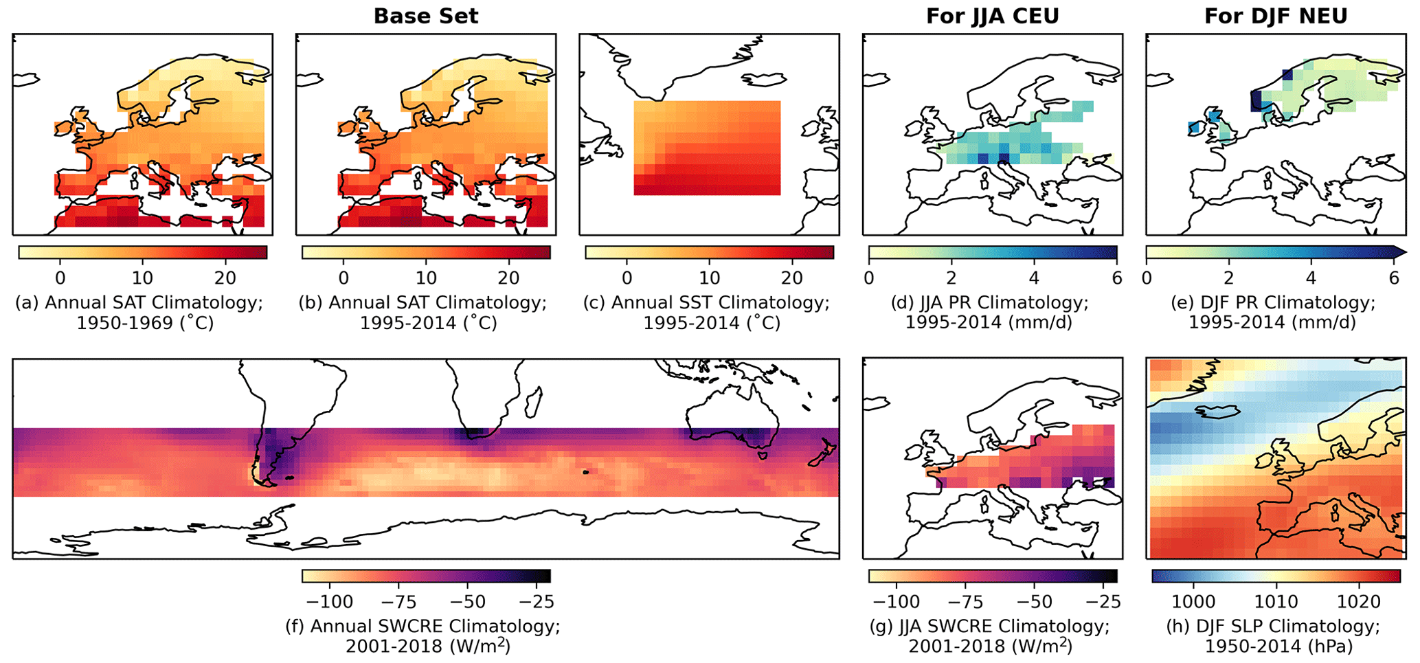
Figure 5 Observed predictor fields used to determine model performance for European climate applications in ClimSIPS; a base set used in both cases includes (a) annual average Berkeley Earth Surface Temperature (BEST) European SAT climatology (1950–1969), (b) annual average BEST European SAT climatology (1995–2014), (c) annual average NOAA Extended Reconstructed Sea Surface Temperature version 5 (ERSSTv5) North Atlantic sea surface temperature (SST) climatology (1995–2014), and (f) annual average Clouds and the Earth’s Radiant Energy System (CERES) Southern Hemisphere midlatitude shortwave cloud radiative effect (SWCRE) climatology (2001–2018). For June–July–August (JJA) central European (CEU) applications, (d) JJA average E-OBS gridded central Europe station PR climatology (1995–2014) and (g) JJA CERES CEU SWCRE climatology (2001–2018) are added to the base set. For December–January–February (DJF) northern European (NEU) applications, (e) DJF average E-OBS gridded northern Europe station PR climatology (1995–2014) and (h) DJF NOAA-CIRES-DOE 20th Century Reanalysis V3 (NOAA-20C) North Atlantic sector sea-level pressure (SLP) climatology (1950–2014) are added to the base set.

5.2 Spread in projected European temperature and precipitation change

Spread, the third and final dimension of ClimSIPS, differs from independence and performance because it is explicitly based on targeted future model outcomes rather than on historical model properties. While it is important for users to recognize that without independence, model agreement is meaningless, and without performance, uncertainty in future projections can be excessive, it is also important they have the opportunity to sample novel climate outcomes if their application so requires. To allow users to maximize climate change signal diversity, we define spread as the distance between models in normalized JJA-CEU- and DJF-NEU-averaged SAT and PR change space, with change, as previously stated, referring to the difference between 2041–2060 and 1995–2014 mean state values in SSP5-8.5 and RCP8.5. Normalization (subtracting the ensemble mean and dividing it by the ensemble standard deviation) is carried out within CMIP5 and CMIP6 separately and ensures that SAT and PR distances contribute equally to the spread metric S_ij. With normalized SAT and PR change for each model, abbreviated as SATΔ and PRΔ, respectively, spread distance between models i and j is

$$\begin{array}{}\text{(5)}& S_{ij}=\sqrt{(\text{SAT}{\mathrm{\Delta }}_i-\text{SAT}{\mathrm{\Delta }}_j{)}^{\mathrm{2}}+(\text{PR}{\mathrm{\Delta }}_i-\text{PR}{\mathrm{\Delta }}_j{)}^{\mathrm{2}}}.\end{array}$$

The only remaining complexity to computing spread is deciding on model representation in an ensemble where some models contribute multiple members. Two strategies are explored. In the first, models with multiple ensemble members are represented by their ensemble mean SAT and PR changes, alongside their individually represented counterparts. In the second, all models are represented by an individual ensemble member chosen such that overall spread within the ensemble is at a maximum (i.e., is farthest from all other members already placed in SAT–PR change space). We select spread-maximizing members from models in a manner similar to the KKZ algorithm (Katsavounidis et al., 1994). First, all individually represented models are placed in SAT–PR change space. Next, the model ensembles are assessed one by one, and the member farthest from all already placed models is chosen. Because member selection is done iteratively, there are multiple possible spread-maximizing solutions; here we focus on one solution obtained by selecting from model ensembles in alphabetical order. Further details of individual member selection are provided in Sect. S5. We apply these two representation strategies to the performance and independence metrics as well and enter into ClimSIPS with a set of 34 CMIP6 models (Table 1) and 26 CMIP5 models (Table 2), each with a scalar performance score (P_i) and vectors of intermember (from Part I; I_ij) and spread (S_ij) distances to all other models in the ensemble.

5.3 Cost function and subselection triangle

With independence, performance, and spread metrics computed for each model, ClimSIPS can be carried out via a cost function minimization scheme. The first step of ClimSIPS is for the user to decide the number n of selections (s_i) they would like to make from a selection pool of N available models (s₁,…s_N). In this study, we demonstrate the method by selecting subsets of varying sizes n from selection pools of varying sizes N, henceforth referred to as a “N-choose-n subselection”. To illustrate the method, we select two model simulations, s₁ and s₂, from a purposefully reduced five-model selection pool, s₁,…s₅, in a 5-choose-2 subselection. We then explore method sensitivities and recommendation strategies with a 34-choose-3 subselection for CMIP6 central European summer case. Lastly, to suit a broader range of applications, we report and recommend five-model subsets for the central European summer and northern European Winter cases from CMIP6 (N=34). The CMIP5 26-choose-5 subselection is also provided in Sect. S6.

Once a subset size is decided upon by the user, ClimSIPS proceeds to compute the value of a cost function for each possible combination of n selections. Comprised of a performance term, $\mathcal{P}(s_{\mathrm{1}},..s_n)$; an independence term, ℐ(s₁,…s_n); and a spread term, 𝒮(s₁,…s_n), the cost function is

$$\begin{array}{}\text{(6)}& \begin{array}{rl}{C}_{\mathit{\alpha },\mathit{\beta }}(s_{\mathrm{1}},\mathrm{\dots }{s}_n)& =(\mathrm{1}-\mathit{\alpha }-\mathit{\beta })\cdot \mathcal{P}(s_{\mathrm{1}},\mathrm{\dots }{s}_n)\\ & -\mathit{\alpha }\cdot \mathcal{I}(s_{\mathrm{1}},\mathrm{\dots }{s}_n)-\mathit{\beta }\cdot \mathcal{S}(s_{\mathrm{1}},..s_n).\end{array}\end{array}$$

The importance to the user of 𝒫(s₁,…s_n), ℐ(s₁,…s_n), and 𝒮(s₁,…s_n) is determined by two parameters, α and β. Both parameters range from 0 to 1; α sets the importance of independence, and β sets the importance of spread. The importance of performance, $\mathrm{1}-\mathit{\alpha }-\mathit{\beta }$ is a trade-off based on the importance of the other two terms that cannot be negative, thus requiring that $\mathit{\alpha }+\mathit{\beta }\le \mathrm{1}$. For each pair of α and β values, there is a combination of models that minimizes the cost function based on their combined values of 𝒫(s₁,…s_n), ℐ(s₁,…s_n), and 𝒮(s₁,…s_n).

Because each model has a scalar performance score P_i, 𝒫(s₁,…s_n) is defined as the sum of the normalized P_i values in each subset:

$$\begin{array}{}\text{(7)}& {\displaystyle }{\displaystyle }\mathcal{P}(s_{\mathrm{1}},\mathrm{\dots }{s}_n)=\sum _{k=\mathrm{1}}^n{\displaystyle \frac{P_{s_k}-{\stackrel{\mathrm{‾}}{\mathit{P}}}_{s_{\mathrm{1}},\mathrm{\dots }{s}_N}}{\mathit{\sigma }\left({\mathit{P}}_{s_{\mathrm{1}},..s_N}\right)}}.\end{array}$$

P_i values are normalized by subtracting the selection pool mean value ${\stackrel{\mathrm{‾}}{\mathit{P}}}_{s_{\mathrm{1}},\mathrm{\dots }{s}_N}$ and dividing it by the selection pool standard deviation $\mathit{\sigma }\left({\mathit{P}}_{s_{\mathrm{1}},\mathrm{\dots }{s}_N}\right)$. The term is positive in the cost function because lower values of P_i indicate smaller biases and thus higher performance. If a user prefers to select based on model performance only (α=0, β=0), the set of n highest-performing models will minimize the cost function.

Model independence and spread metrics, ℐ(s₁,…s_n) and 𝒮(s₁,…s_n), are based on the I_ij and S_ij distance matrices of the selected model subsets. The distances are normalized by the mean and standard deviation of their entire selection pool distance matrices (${\mathbf{I}}_{s_{\mathrm{1}},\mathrm{\dots }{s}_N,s_{\mathrm{1}},\mathrm{\dots }{s}_N}$ and ${\mathbf{S}}_{s_{\mathrm{1}},\mathrm{\dots }{s}_N,s_{\mathrm{1}},\mathrm{\dots }{s}_N}$, respectively) and then summed over half of the matrix to avoid double counting:

$$\begin{array}{}\text{(8)}& {\displaystyle }& {\displaystyle }\mathcal{I}(s_{\mathrm{1}},..s_n)=\sum _{k<l}^n{\displaystyle \frac{I_{s_k,s_l}-{\stackrel{\mathrm{‾}}{\mathbf{I}}}_{s_{\mathrm{1}},..s_N,s_{\mathrm{1}},..s_N}}{\mathit{\sigma }\left({\mathbf{I}}_{s_{\mathrm{1}},..s_N,s_{\mathrm{1}},..s_N}\right)}}\text{(9)}& {\displaystyle }& {\displaystyle }\mathcal{S}(s_{\mathrm{1}},..s_n)=\sum _{k<l}^n{\displaystyle \frac{S_{s_k,s_l}-{\stackrel{\mathrm{‾}}{\mathbf{S}}}_{s_{\mathrm{1}},..s_N,s_{\mathrm{1}},..s_N}}{\mathit{\sigma }\left({\mathbf{S}}_{s_{\mathrm{1}},..s_N,s_{\mathrm{1}},..s_N}\right)}}.\end{array}$$

In the cost function, $\mathcal{I}(s_{\mathrm{1}},..s_n)$ and $\mathcal{S}(s_{\mathrm{1}},..s_n)$ are negative terms because larger distances between models correspond to higher levels of independence and spread, which, along with higher performance, are the subset properties we prioritize. As independence and/or spread increases within a subset, the larger negative $\mathcal{I}(s_{\mathrm{1}},..s_n)$ and $\mathcal{S}(s_{\mathrm{1}},..s_n)$ terms eclipse the $\mathcal{P}(s_{\mathrm{1}},..s_n)$ term, leading to a more and more negative minimum value of the cost function.

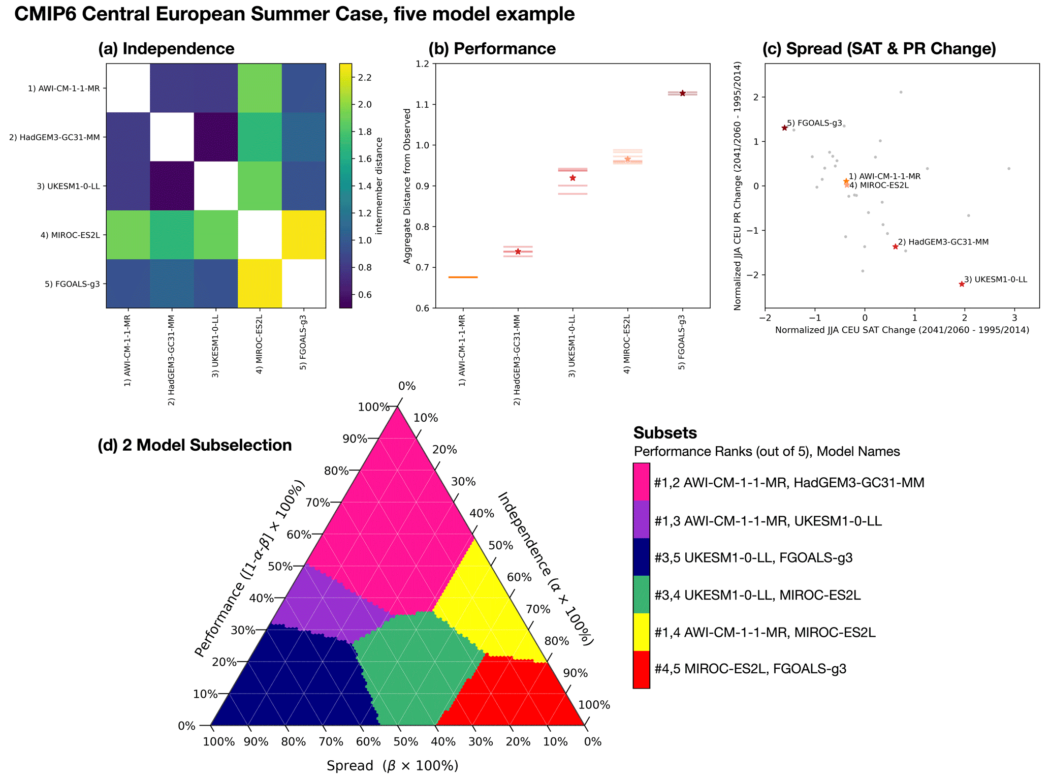
Figure 6 Five models from CMIP6 are used to illustrate ClimSIPS for JJA CEU applications. Independence, defined by intermember distances (Fig. 3), for the five models is shown in panel (a). Performance, defined as the average of model-observed RMSE for the six JJA CEU predictors (Fig. 5), is shown in panel (b). Lower values indicate a model is close to observed and thus higher-performing for the task. Performance of individual ensemble members is shown as horizontal lines, and ensemble mean performance is starred. In panel (c), the five selected models are highlighted among CMIP6 ensemble means (gray dots; single members where appropriate) in normalized JJA CEU SAT and PR change (SATΔ and PRΔ, respectively; 2041/2060–1995/2014 in SSP5-8.5) space. The target values are normalized by subtracting the CMIP6 mean and dividing it by the CMIP6 standard deviation. Panel (d) shows the “subselection triangle” ternary contour plot. Selected subsets (colored regions) minimize a performance–independence–spread cost function as varying degrees of importance are placed on performance (1-α-β), independence (α), and spread (β). Subsets are listed by performance rank (out of 5) and model name on the color bar to the right of the triangle.

As previously discussed, different sets of models minimize the cost function for different values of α and β. To summarize how different subsets map to different priorities, we utilize a “subselection triangle” ternary contour plot (Harper et al., 2015). Ternary plots represent three-component systems that require the component contributions together to sum to a constant, typically 100 %. The requirement, which reduces the degrees of freedom in the system from 3 to 2, allows component value combinations to be plotted on an equilateral triangle with angled axes along each side. As the cost function balances the relative importance of independence (α), performance (1-α-β), and spread (β), it is an ideal candidate for such a visual representation.

We introduce the subselection triangle in a toy example of subselection: choosing two out of five CMIP6 models for JJA CEU applications (Fig. 6). Of the five models in the selection pool, AWI-CM-1-1-MR is represented by its single member, while HadGEM3-GC31-MM, UKESM1-0-LL, MIROC-ES2L, and FGOALS-g3 are represented by their ensemble means. The models were chosen because they span a range of independence (Fig. 6a), performance (Fig. 6b), and spread (Fig. 6c) within CMIP6 and therefore can help illustrate how the cost function selects subsets based on the different priorities. Intermember distances between the models in the selection pool (Fig. 6a) highlight the low level of independence between family members HadGEM3-GC31-MM and UKESM1-0-LL and the high level of independence of MIROC-ES2L with respect to all other models, as discussed in Part I. Performance scores, shown for each ensemble member (Fig. 6b, horizontal lines) and ensemble means (Fig. 6b, stars), lend themselves to an ordered rank of the models from no. 1 (AWI-CM-1-1-MR) to no. 5 (FGOALS-g3). Placing each model in normalized SAT–PR change space (Fig. 6c) demonstrates the spread in future climate outcomes possible within the selection pool (labeled stars) and with CMIP6 overall (gray dots). Notably, AWI-CM-1-1-MR and MIROC-ES2L, two relatively independent models, project near-identical changes in SAT and PR mean states by the mid-century, while family members HadGEM3-GC31-MM and UKESM1-0-LL do not.

In Fig. 6d, selected subsets are represented by colored regions of the subselection triangle. Boundaries between selected subsets are determined by the distributions of independence, performance, and spread within the selection pool and by the step resolution on which α and β vary. Throughout the study, we vary α and β from 0 to 1 (in concert) in steps of 0.01. In the five-model example, six two-model combinations (out of a possible 10 combinations) minimize the cost function as α and β vary in this way.

The subselection triangle is best investigated first along its boundaries. At each vertex, one property is given 100 % priority, and along each edge, only two priorities are balanced. At the top vertex, 100 % priority is given to performance (α=0, β=0), as indicated by the axis that runs down the left edge of the triangle. Along the left edge from top to bottom, the importance of performance diminishes, while the importance of spread increases to reach 100 % priority at the left vertex (α=0, β=1). Along the bottom edge (the spread axis), the trade-off shifts to be between spread and independence, with independence being given 100 % priority at the right vertex (α=1, β=0). Finally, from bottom to top along the independence axis (the right edge of the triangle), the importance of independence diminishes, while the importance of performance increases.

Regions that intersect with vertices or edges can then be characterized according to priority. In Fig. 6d, the magenta region that intersects with the triangle's top vertex is the subset of the highest-performing models, AWI-CM-1-1-MR and HadGEM3-GC31-MM, as indicated by the color bar labeled with performance ranks out of 5. From the point where performance and spread are each given 50 % priority, AWI-CM-1-1-MR and UKESM1-0-LL minimize the cost function (purple region). The blue region, intersecting with the left vertex, is comprised of the models furthest apart in normalized SAT–PR change space, UKESM1-0-LL and FGOALS-g3 (Fig. 6c). In the green region, independence rather than performance takes priority alongside spread, resulting in a subset of the no. 3 and no. 4 ranked models, UKESM1-0-LL and MIROC-ES2L. Overall, if independence is prioritized, the cost function is likely to select subsets containing the independent MIROC-ES2L, as seen in the red and yellow regions of the subselection triangle. For the yellow region, the balance between performance and independence happens to yield a subset of models with little spread (AWI-CM-1-1-MR and MIROC-ES2L). Assigning no priority to a certain property does not necessarily mean the subset will be lacking in it; the other two subsets that fall along the independence axis (Fig. 6 magenta and red regions) do have reasonable levels of model spread. However, without some level of priority given to a property, there is no guarantee it will be sufficiently represented.

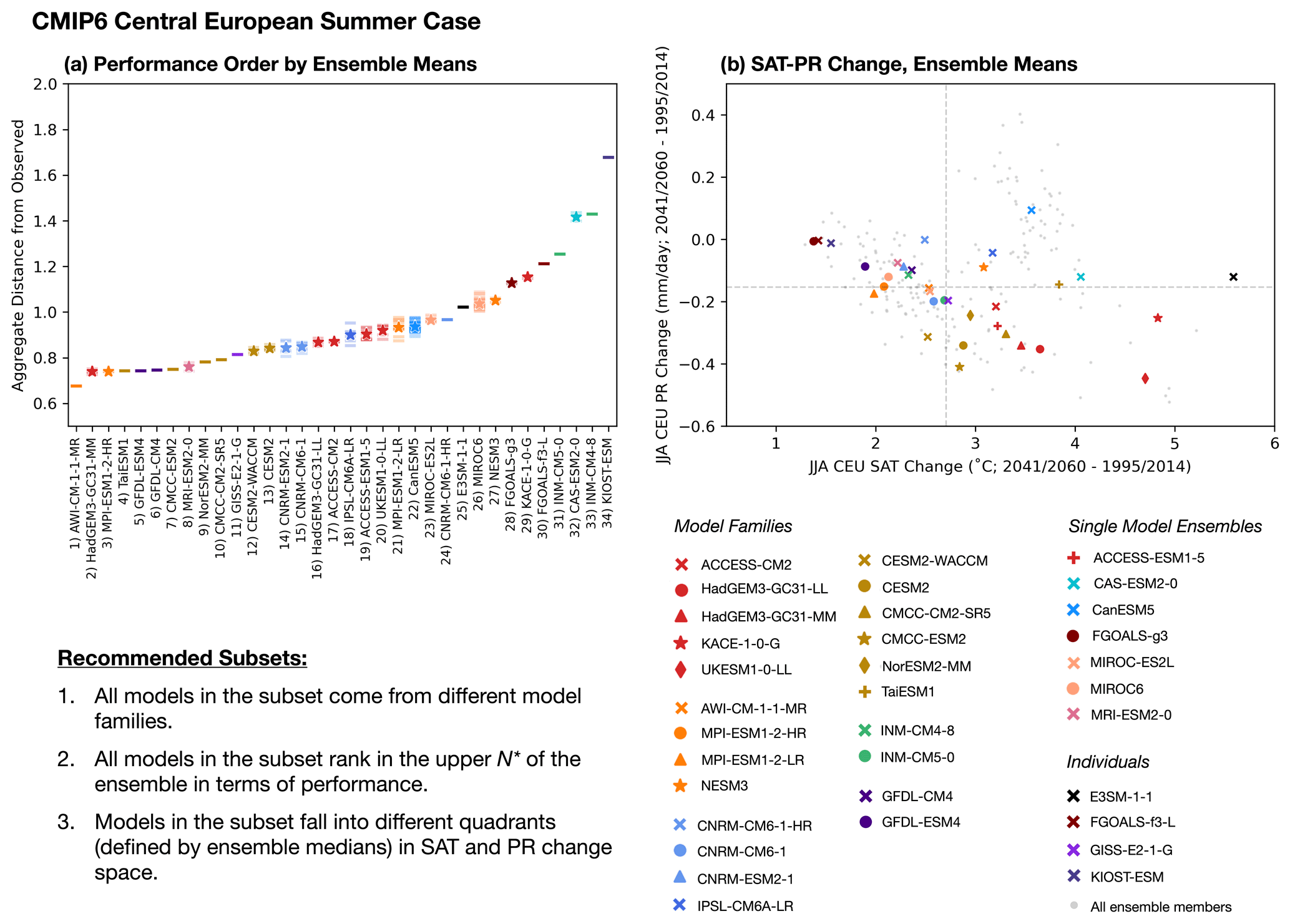
Figure 7 Independence, performance, and spread criteria that underpin model subset recommendations used throughout the remainder of the study. For independence, we recommend all models in a subset come from different model families (listed in the legend below panel b). For performance, we recommend all models in a subset rank in the upper N^* of the ensemble with N^* left up to user discretion. Performance in the full CMIP6 ensemble for JJA CEU applications is shown in panel (a) in terms of the aggregated distance from the observed, a metric based on the average of model-observed RMSE for the six JJA CEU predictors shown in Fig. 5. Higher performers have a lower aggregated distance from the observed, and performance order is based on ensemble mean performance (stars) where applicable, i.e., when a model is represented by more than one ensemble member. Horizontal lines represent the performance of individual ensemble members. For spread, we recommend models within the subset fall into the different quadrants of JJA CEU SAT and PR change space. JJA CEU SAT and PR change (2041/2060–1995/2014 for SSP5-8.5) values for each ensemble member of CMIP6 (light-gray dots) and for ensemble means (colored markers) are shown in panel (b). Dashed gray lines indicate the median JJA CEU SAT and PR change value within the ensemble of ensemble means and separate the ensemble into four quadrants.

5.4 Recommended subsets for European applications

Selecting more models from a larger selection pool leads to an increase in subsets composed of different models, minimizing the cost function as α and β vary. Subselection triangles become more complex and subdivided when three- and five-model subsets are selected from full CMIP ensembles; the six selected subsets from the 5-choose-2 CMIP6 JJA CEU example shown in Fig. 6 become 37 selected subsets in the CMIP6 JJA CEU 34-choose-3 subselection by ensemble mean and 45 selected subsets in the 34-choose-5 subselection by individual member. The size, shape, and number of regions within the subselection triangle are determined by independence, performance, and spread distributions; the larger the selection pool, the more difficult it becomes to predict the combination of models that will minimize the cost function. A subset can minimize the cost function for a small region in α–β space or even a single value of α and β. Small subset regions are as valid as larger ones; they simply reflect that independence, performance, and spread are distributed such that there are several model combinations in contention to minimize the cost function in that region of the subselection triangle. Conversely, when a subset minimizes the cost function for a large region of the subselection triangle, it suggests that it is comprised of outliers given priority in the cost function to such an extent that other model combinations cannot reach the minimum.

To help users decide which subset is best suited to their needs, we provide recommendations based on independence, performance, and spread criteria that go further than contribution percentages. Recommendation criteria are listed in Fig. 7 in conjunction with CMIP6 JJA CEU performance and (non-normalized) SAT–PR change distributions for models represented by ensemble means. The objective of these recommendation criteria is to further screen out selected sets that do not meet the following specific (user-defined) desirable properties. The criteria are as follows:

1. All models in the subset come from different model families.

2. All models in the subset rank in the upper N^* of the ensemble in terms of performance.

3. Models in the subset fall into the different quadrants (defined by ensemble medians) in SAT and PR change space. For subsets of four or more models, all quadrants must be represented.

For the independence criteria, model families defined in Part I are used as an independence guideline. For the performance criteria, the threshold N^* is left up to user discretion; we choose different thresholds for the different regional and seasonal cases to accommodate different performance distributions. For the spread criteria, we adapt the strategy of Ruane and McDermid (2017) and separate SAT–PR change space into quadrants with respect to ensemble medians. By recommending subsets of models that occupy the (relatively) cool–wet, cool–dry, warm–wet, and warm–dry margins of the ensemble, we ensure not only spread but also a set of diverse future climate outcomes.

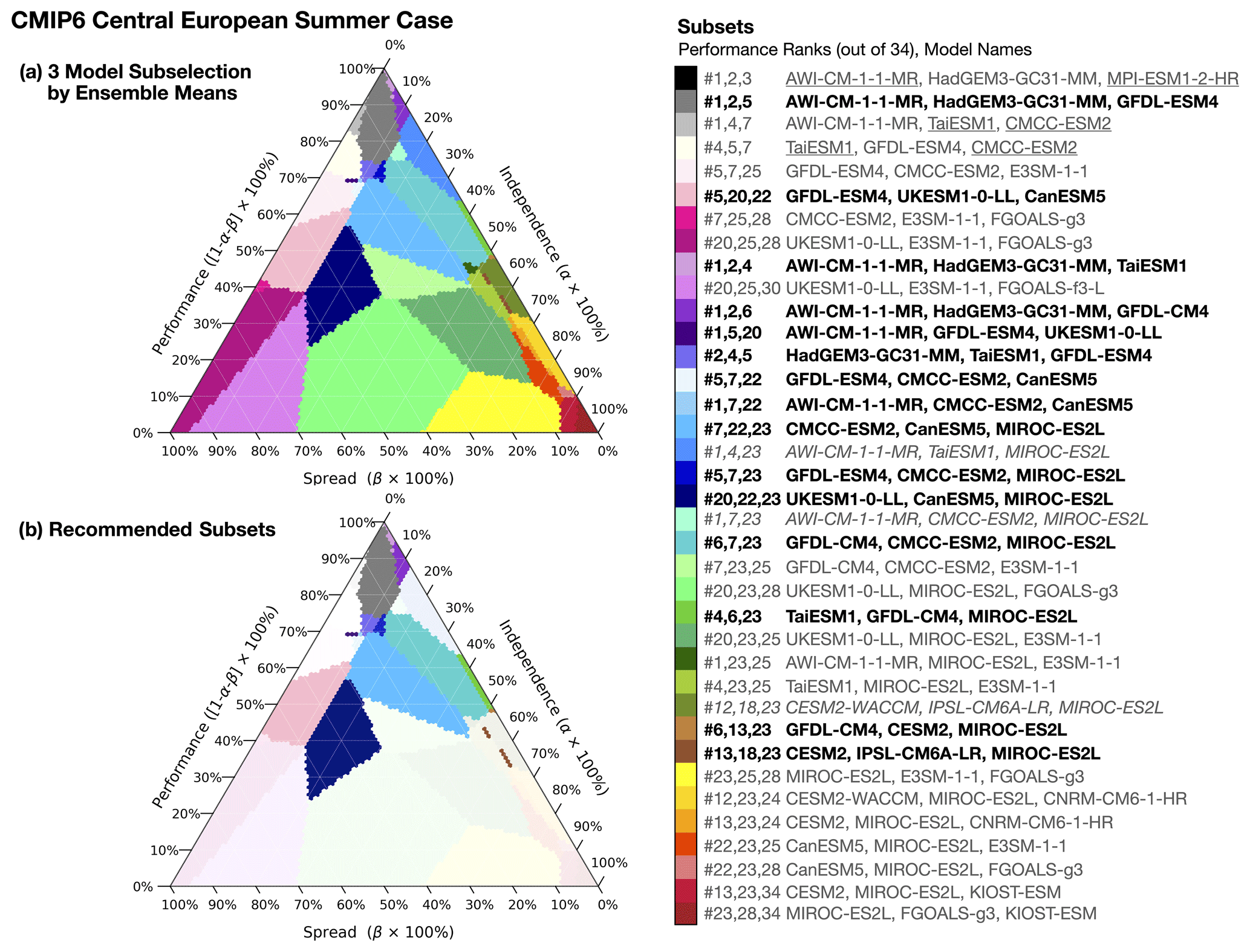
Figure 8 Ternary subselection triangles of the three-model subselection from the full CMIP6 ensemble for JJA CEU applications. Each model is represented by its ensemble mean (or individual member when applicable). A total of 37 three-model subsets minimize the independence–performance–spread cost function for different values of α and β (a). Models within each subset are listed with their performance rank (out of 34). Of the 37 possible subsets, we recommend 15 (panel b; labeled in bold) based on the following criteria: (1) all models in the subset come from different model families, (2) all models in the subset have a performance rank at or above 23 out of 34, and (3) all models in the subset come from different quadrants in JJA CEU SAT and PR change space. Remaining subsets that fail the performance criteria are listed in gray; those that fail the independence criteria are listed in gray with model family members underlined. Subsets that fail the spread criteria are indicated in italics.

In Fig. 7a, for models with multiple members, performance metrics are ordered by ensemble mean value (star markers), which are superimposed on the performance metrics of individual members (horizontal lines). The JJA CEU performance distribution in CMIP6 reflects the fact that most of the models in the ensemble are not significantly biased with respect to observations, though several models are biased enough to form a perceptible tail. This implies that most CMIP6 models meet the basic standards to be considered suitable for downstream climate applications and allows us to set the N^* threshold to be more inclusive than exclusive. Overall, individual member performance is tightly clustered around its ensemble mean for each model; this is true for all cases we explore in this study (see Fig. S11). The tight clustering confirms that performance is a model property rather than a member property. When defined by climatological predictors, performance is not just a matter of chance that observations match some members but not others due to internal variability. Tight clustering also means that representing models by ensemble mean versus an individual member will not fundamentally change performance order, aside from a few minor shifts up or down for models in the heart of the distribution.

In Fig. 7b, ensemble means (colored markers) and all CMIP6 ensemble members (gray dots) are placed within raw JJA CEU SAT–PR change space. Without normalization, it is clear that there is a wide range of JJA CEU SSP5-8.5 mid-century warming in CMIP6 models from 1.37 to 5.59 ^∘C. However, models on both ends of the warming spectrum tend to be lower than average in terms of performance, suggesting these best- and worst-case warming projections may not be as realistic as the projections within the approximately 2–4 ^∘C warming range populated by the bulk of the CMIP6 ensemble. In terms of precipitation change, only CanESM5 (Fig. 7b, bright-blue cross marker) has an ensemble mean projecting wetter conditions in the region by the mid-century; all other models project little change or an overall central European summer drying. The joint SAT–PR change distribution is separated into a less warming–less drying quadrant containing 10 models, a less warming–more drying quadrant containing 7 models (including MPI-ESM1-2-HR, which has a value slightly below the PR change ensemble median), a more warming–more drying quadrant containing 11 models, and a more warming–less drying quadrant containing 6 models. Model labels, listed below Fig. 7b, are grouped in terms of their designations determined in Part I: as model families, single-model ensembles, or individuals. In two of the six model families, all family members reside in the same quadrant; models with a MetUM-HadGEM3-GA7.1 atmosphere (Fig. 7b dark red) all warm and dry more than the ensemble median, while the two GFDL model variants both warm and dry less than the ensemble median (Fig. 7b dark purple). The remaining model families each span two to three quadrants, demonstrating that model dependence is not necessarily clearly correlated with spread in projected outcome because internal variability and parameter perturbations influence the latter.

With independence, performance, and spread metrics defined, the CMIP6 JJA CEU 34-choose-3 subselection, with models represented by the ensemble mean, is presented in Fig. 8. While stepping through α and β, 37 three-model combinations minimize the cost function, from the three highest performers (Fig. 8a black region; AWI-CM-1-1-MR/HadGEM3-GC31-MM/MPI-ESM1-2-HR) to the three most independent models (Fig. 8a dark-red region; MIROC-ES2L/FGOALS-g3/KIOST-ESM) to the three models furthest from each other in SAT–PR change space (Fig. 8a dark-magenta region; UKESM1-0-LL/E3SM-1-1/FGOALS-g3). The subsets that minimize the cost function between those 100 % priority cases are labeled by model performance rank (out of 34) triplet and model names (Fig. 8, color bar). Note that model performance rank is used here specifically as a shorthand for comparing constituents across subsets, not as a commentary on how much better performing one model is than another model. Most models in the ensemble have a similar level of performance (Fig. 7a), allowing us to set the recommendation performance threshold N^* to include models in the top two-thirds of the ensemble, ranked up to and including no. 23 out of 34.

Applying all three recommendation criteria results in 15 recommended subsets (Fig. 8b), which are listed as color bar labels in black. For reference, all subsets recommended throughout the study are cataloged in Tables S5 and S6. Of the remaining subsets, those listed in gray do not satisfy one or more of the recommendation criteria. The same model family representation within a subset is indicated with family members underlined. Subsets that include one or more model with a performance rank between no. 24 and no. 34 are listed in plain gray text, while subsets that have more than one model in the same SAT–PR change quadrant are listed in italics. There is a higher likelihood of selecting two models from the same model family in subsets comprised of high-performing models. Mirroring the finding of Sanderson et al. (2017) that high-performing CMIP5 models tended to be less independent and have more near replicates in the archive, the relationship between performance and independence we find in CMIP6 suggests that the global-scale SAT and SLP climatological differences that bestow independence also manifest as local and regional-scale model biases that diminish performance.

In the CMIP6 JJA CEU 34-choose-3 subselection by ensemble means, recommended subsets (Fig. 8b) are comprised either solely of members of model families or a combination of model family members with the independent MIROC-ES2L and/or unique in SAT–PR change space CanESM5. In total, recommended subsets cover 15 % of the subselection triangle. Models with a CAM-based atmosphere (TaiESM1, CMCC-ESM2, and CESM2) are included in 10 of the 15 recommended subsets, GFDL variants (GFDL-CM4 and GFDL-ESM4) are included in 9, and MIROC-ES2L is included in 7. Together, the three groupings form 4 of the 15 subsets. Models with a MetUM-HadGEM3-GA7.1 atmosphere (HadGEM3-GC31-MM and UKESM1-0-LL) and the ECHAM6.3-based AWI-CM-1-1-MR are also well represented within the recommended subsets, appearing in six and five subsets, respectively. AWI-CM-1-1-MR and HadGEM3-GC31-MM tend to be chosen as family representatives because they are ranked first and second in performance in the ensemble. UKESM1-0-LL, which features the largest mid-century joint change in JJA CEU SAT and PR in the ensemble, takes over for HadGEM3-GC31-MM as its family's representative when the importance of performance drops below approximately 70 %. Small recommended subset regions (<10 pixels in α–β space) occur at approximately 70 % performance, 10 % independence, and 20 % spread, likely because performance priority has reduced enough to allow spread outliers like UKESM1-0-LL and CanESM5 to be in contention alongside various models within the core of the performance distribution. Similarly, small recommended subset regions near 50 % performance and 50 % independence result from the selection of various models in the performance core with the independent MIROC-ES2L.

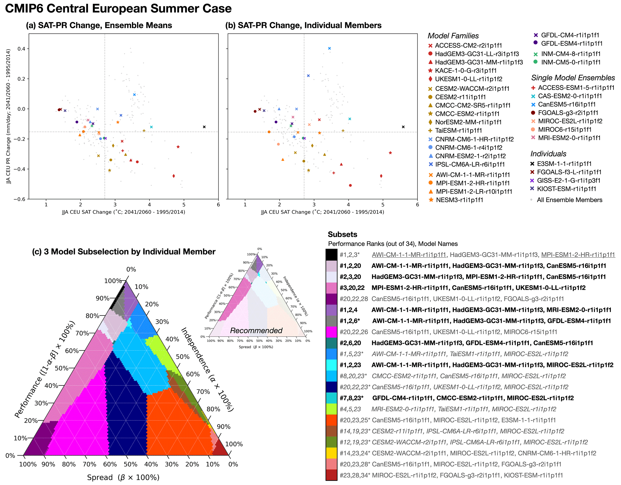
Figure 9 Three model subselection for CMIP6 JJA CEU applications with all models represented by an individual ensemble member. CMIP6 JJA CEU SAT–PR change (not normalized) for ensemble mean representation (as in Fig. 7b) versus individual member representation are shown in panels (a) and (b), respectively. Colored markers, indicating model representation, are superimposed on all CMIP6 ensemble members (light-gray dots). Individual ensemble members are labeled in the key and were selected to maximize spread. In both panels, ensemble median values for JJA CEU SAT and PR change (gray dashed lines) delineate the four quadrants used for spread recommendations. The full and recommended (inset) subselection triangles for three-model subselection by individual member are shown in panel (c). As in Fig. 8, recommended subsets are labeled in black. Subsets labeled in gray contain one or more models (1) that come from the same model family (underlined), (2) that fall below the performance threshold, or (3) that fall within the same quadrant of SAT–PR change space (italic). Additionally, common subsets in ensemble mean-based subselection (Fig. 8) and individual member-based subselection share common colors; these subsets in common are also labeled with a starred performance rank triplet.

For use cases that require recommendations of specific simulations, we also run ClimSIPS with each model represented by an individual member. For subselection by ensemble mean, some models are represented by a member, while others are represented by an average. This representational difference is less of an issue for the independence and performance metrics, which both are intentionally designed such that ensemble members do not deviate far from their ensemble mean values. For the spread metric, however, an individual climate change projection and an average across a set of climate change projections are unlikely to be equivalent due to internal variability. For example, a model's range of projected climate outcomes may include interesting outlier cases that are curtailed by ensemble averaging. Using the ensemble mean as representation then does not capture the model's full “spread potential” or ability to differentiate itself within the ensemble. For a model represented by only one member, the projection provided as representation could fall anywhere within the model's un-sampled SAT–PR change distribution; there is no way to know if it sits near to and thus reflects the model's hypothetical ensemble mean.

Figure 9 summarizes how individual member representation affects the CMIP6 JJA CEU 34-choose-3 subselection, predominately by amplifying model spread. When given the choice among ensemble members, the method selects outlier cases to represent models to provide users interested in novel climate outcomes with not just a model but a specific projection that may be of interest. Compared to ensemble mean representation (Fig. 9a), individual member representation (Fig. 9b) provides an increase, in CMIP6 JJA CEU PR change spread in particular, including an additional projection of wetter future JJA CEU conditions (IPSL-CM6A-LR-r6i1p1f1) and fewer model overlaps in the core of the ensemble. There is not a substantial increase in the range of JJA CEU SAT change in CMIP6, due to the fact that high and low change projections come from individually represented models. To evaluate whether these differences were CMIP6 JJA CEU-specific, we also compare ensemble mean representation to that of spread-maximizing members for the CMIP6 DJF NEU (Fig. S12), CMIP5 JJA CEU (Fig. S13), and CMIP5 DJF NEU (Fig. S14) cases. Similar to the CMIP6 JJA CEU case, CMIP5 JJA CEU PR change spread increases more than SAT change spread when models are represented by an individual member versus an ensemble mean. In both CMIP6 and CMIP5 DJF NEU cases, however, the SAT change spread increase is more striking than the PR change increase (Fig. S12).

The additional distance between models in SAT–PR change space afforded by individual member representation serves to simplify the CMIP6 JJA CEU 34-choose-3 subselection triangle (Fig. 9c). The number of cost function-minimizing model subsets decreases from 37 subsets with 15 recommended when models are represented by ensemble mean (Fig. 8) to 21 subsets with eight recommended when models are represented by individual members (Fig. 9c). The two strategies share 12 subsets in common, which are indicated by regions of common color in Figs. 8a and 9c and by starred model rank triplets in the color bar labels of Fig. 9c. Though some model ranks have shifted up or down due to the change in representation, the same set of 23 out of 34 models meet the performance threshold in both cases. Of the 12 shared subsets, two are recommended in both cases (Figs. 8a, 9c dark gray and teal), while three are recommended in ensemble mean subselection but not in individual member subselection (Figs. 8a, 9c dark sky blue, dark blue, and dark brown). This recommendation difference is due to MIROC-ES2L shifting from the less warming–more drying quadrant to the more warming–less drying quadrant when represented by member r1i1p1f2 (Fig. 9a, b salmon cross marker). The remaining recommended individual member subsets feature many of the same models/model families as in the ensemble mean case. A comparison of $\mathcal{I}(s_{\mathrm{1}},..s_n)$, $\mathcal{P}(s_{\mathrm{1}},..s_n)$, and $\mathcal{S}(s_{\mathrm{1}},..s_n)$ component contributions to the minimized cost function, shown separately in Fig. S15, confirms the two representations have qualitatively similar gradients in component magnitude within the subselection triangle. Because the two strategies yield similar results in our CMIP6 JJA CEU test case and because individual member representation has the additional advantage of guiding users to specific simulations, we move forward to five-model subselection by individual members for each of the European case studies, shown as subselection triangles in Figs. 10 and S16.

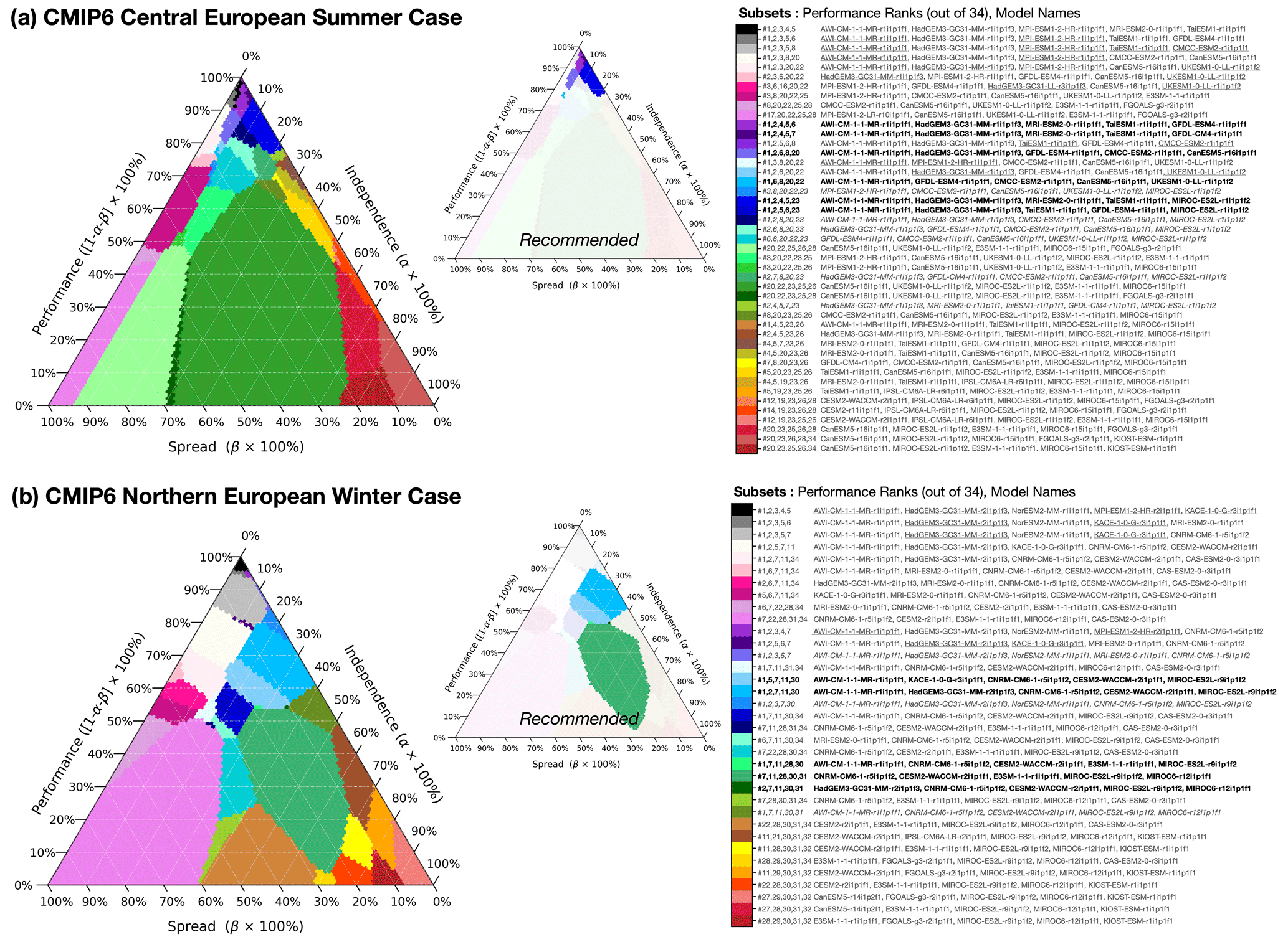
Figure 10 Ternary diagrams of the five-model subselection for CMIP6 (a) JJA CEU and (b) DJF NEU applications. Each model is represented by an individual member, listed in the legend. Similarly to Fig. 9, each case is shown alongside a subset recommendation triangle. Of the CMIP6 JJA CEU case's 45 possible subsets, 6 are recommended based on a performance rank threshold of 23 out of 34. For the CMIP6 DJF NEU case, 5 of 35 possible subsets are recommended based on a performance rank threshold of 31 out of 34.

Combinations of five models add further complexity to the CMIP6 JJA CEU subselection triangle (Fig. 10a); 45 out of a possible 278 256 subsets minimize the cost function at different points in α–β space. We recommend six subsets based on the same recommendation criteria used in CMIP6 JJA CEU three-model subselection, with the additional condition that all four SAT–PR change quadrants are represented by the five models. All recommendations include AWI-CM-1-1-MR-r1i1p1f1 from the ECHAM6.3-based family (Fig. 3a orange), one simulation with a MetUM-HadGEM3-GA7.1 atmosphere (HadGEM3-GC31-MM-r1i1p1f3 or UKESM1-0-LL-r1i1p1f2), and a representative from the CAM-based model family (Fig. 3a goldenrod; TaiESM1-r1i1p1f1 or CMCC-ESM2-r1i1p1f1). GFDL variants (Fig. 3a purple) also appear in five of the six recommended subsets, suggesting that those four-model families comprise a reasonable, independent subset spanning a range of climate outcomes for CMIP6 JJA CEU applications. Depending on user needs, the highly independent MIROC-ES2L-r1i1p1f2; relatively less-biased MRI-ESM2-0-r1i1p1f1; or CanESM5-r16i1p1f1, which is one of few that project wetter future JJA CEU conditions, should also be considered.

Because region- and season-specific performance and spread metrics are used for each case, different CMIP6 subsets feature in the subselection triangle for northern European winter applications (Fig. 10b) than for central European summer applications. Individual members chosen to represent models also differ between the DJF NEU and JJA CEU cases due to spread being case-specific. Of the 35 possible subsets that minimize the CMIP6 DJF NEU cost function, no subsets satisfy all three recommendation criteria as developed for JJA CEU applications. This is primarily due to models with performance ranks of 28 to 34 either being highly independent (e.g., no. 30 MIROC-ES2L-r9i1p1f2, no. 31 MIROC6-r12i1p1f1) or unique in projected climate outcome (e.g., no. 28 E3SM-1-1-r1i1p1f1, no. 34 CAS-ESM2-0-r3i1p1f1; see Fig. S11c). In this instance, we therefore chose to relax the performance threshold to consider models with a rank at or above 31 out of 34 to recommend five subsets. For CMIP6 DJF NEU applications, three simulations, CNRM-CM6-1-r5i1p1f2, CESM2-WACCM-r2i1p1f1, and MIROC-ES2L-r9i1p1f2, are included in all recommendations. When performance is given more priority (Fig. 10b blue regions), the three are joined by AWI-CM-1-1-MR-r1i1p1f1 and a simulation with a MetUM-HadGEM3-GA7.1 atmosphere, either HadGEM3-GC31-MM-r2i1p1f3 or KACE-1-0-G-r3i1p1f1. This suggests again that a subset with the large model families individually represented is a good starting point for downstream applications. When priority shifts towards independence and spread (Fig. 10b green regions), subsets tend to include the models with the greatest CMIP6 DJF NEU mid-century positive and negative precipitation changes (E3SM-1-1-r1i1p1f1 and MIROC6-r12i1p1f1, respectively). Though not included in a recommended subset primarily because of performance concerns, CAS-ESM2-0-r3i1p1f1 may also be of interest to some users in search of a CMIP6 DJF NEU worst-case scenario; the simulation warms by 7.82 ^∘C between the 1995–2014 and 2041–2060 base periods (Fig. S12b).

Table 3 Recommended CMIP6 five-model subset by case and primary user priority.

6 Summary, discussion, and conclusion

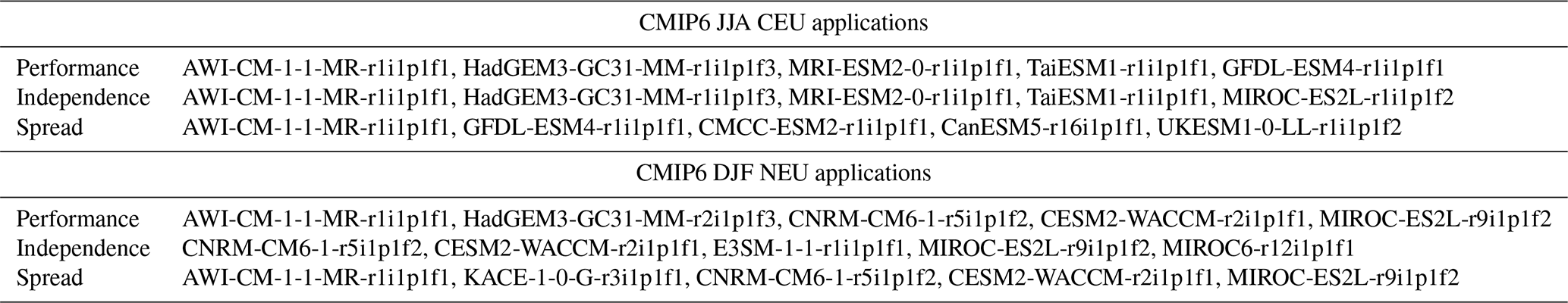
In this study, we developed and demonstrated a method, ClimSIPS, to flexibly select subsets from multi-model ensembles based on the degree to which a user prioritizes model independence, model performance, and spread in projected climate outcomes. During the development of the ClimSIPS, we tested sensitivities and made several refinements to the definition of model dependence in ClimWIP, a performance and independence weighting strategy pioneered in Knutti et al. (2017), which identifies model similarities via the absolute values of historical period, global-scale climatological SAT and SLP predictor fields. Described in Part I, refinements included lengthening predictor climatological averaging periods from 1980–2014 to 1905–2005 and designing predictor spatial fingerprints to explicitly reduce predictor spread within models (e.g., amongst initial-condition ensemble members) while preserving predictor spread between models. Computed separately for SAT and SLP in CMIP5 and CMIP6, the fingerprints spatially masked the 15 % of grid points where ensemble-wide internal variability (defined as the median of the standard deviations within 12 CMIP6 and five CMIP5 initial-condition ensembles) was at a maximum and the 15 % of grid points where the traditional representation of between-model spread (defined as the standard deviation across an ensemble comprised of one ensemble member per model) was at a minimum. An advantage of using climatological SAT and SLP fingerprints rather than unmasked global fields to define model dependence was that masking helps to future-proof against between-model convergence should model developers decide to tune, in particular, the absolute value of global mean surface temperature in models (Mauritsen et al., 2012; Hourdin et al., 2017). The potential for between-model convergence is cited as one of the primary drawbacks of using model output to determine dependence (Annan and Hargreaves, 2017; Brands, 2022b). Additionally, climatological SAT and SLP fingerprints allayed a concern that computing RMSE distance between models does not require the overall collection of intermember distances to meet the formal mathematical definition of metric space (Abramowitz et al., 2019). We found that intermember distances within both CMIP ensembles did satisfy metric criteria, with all sets of three models upholding the triangle inequality of dist(A,B) $<=$ dist(A,C) + dist(C,B). Intermember distances could therefore be both understood as distances and visualized in low-dimensional space.

Updates made to CMIP intermember distances assisted in our effort to make discrete delineations along the spectrum of dependence for three categories: single-model ensembles, model families, and individuals. First and most dependent were single-model ensembles comprised of multiple initial-condition ensemble members, followed by those comprised of both perturbed-physics and initial-condition ensemble members. Next were model families, which we defined as self-contained groups in which all models were within a median intermember distance threshold and were closer to each other than to the rest of the ensemble. We were able to support all family designations with model descriptions and metadata and found our designations to be broadly consistent with other model output and metadata-based dependence definitions (Brands, 2022b). In CMIP6, model families emerged when models shared atmospheric components (e.g., MetUM-HadGEM3-GA7.1 or ECHAM6.3), developed from a shared atmospheric component (e.g., NCAR's CAM), or were variants from the same (e.g., GFDL, EC-EARTH, or INM) or closely collaborating (e.g., CNRM and IPSL) modeling centers. In CMIP5, similar model families were present but with fewer models per family and fewer members per model than in CMIP6. Beyond model families, the last and most independent entities in the CMIP were individuals or uniquely named models represented by a single simulation. The three categories formed a new “representative democracy” within the CMIP, allowing us to explore how a stricter independence definition than the traditional one model, one vote requirement constrained distributions of ECS in CMIP5/6. By applying the new one family, one vote independence constraint, we saw CMIP6's bimodal ECS distribution shift and skew towards lower values of ECS, with the median and the 75th percentile each shifted down by 0.43 ^∘C to 3.44 and 4.29 ^∘C, respectively. CMIP5 ECS, in contrast, maintained its raw distributional form under the one family, one vote independence constraint. Increased representation of certain model families from CMIP5 to CMIP6 explained part of the distributional difference in ECS between the two ensembles; restricting family over-representation reduced the median difference in CMIP5 and CMIP6 ECS by over 60 %. We thus concluded that the increased ECS uncertainty range documented in CMIP6 is, in part, due to the fact that near-identical but differently named models appeared more frequently in CMIP6, and those models tended to have ECS values above 4.5 ^∘C. Crucially, this conclusion could be drawn without any commentary on the quality of CMIP6 models; it simply rested on levels of model representation within the ensemble.

Leveraging the model dependence definition developed in Part I, we demonstrated ClimSIPS for summer and winter European case studies in Part II of this study. Performance was defined in terms of historical biases of concern rather than by historical strengths of unclear merit; we required models to effectively simulate annual climatologies of European SAT, North Atlantic SST, and Southern Hemisphere midlatitude SWCRE, in addition to local summer PR and SWCRE climatologies, for central European summer applications, and local winter PR and regional-scale winter SLP climatologies for northern European winter applications. We found that most models are similarly (and not significantly) biased with respect to observations for the chosen climatological fields. However, in each case, a minority of models had aggregated distances from the observed that were large enough relative to their peers to cast doubt on the projected future European climate states they simulated. These projected future climate states served as the basis of spread, which we defined using each model's JJA CEU or DJF NEU SAT and PR change between present (1995–2014) and mid-century (2041–2060) mean states. Because spread within the CMIP depended on how a model with multiple ensemble members was represented, we explored subselection by ensemble mean and by an ensemble member selected to maximize ensemble spread overall. Depending on user needs, both spread representation strategies may be of interest, the former for studies requiring general model recommendations and the latter for studies in need of specific simulations that project unique climate outcomes.

Subsets were then selected via a cost function, which was optimized for sets of models that were more independent, higher-performing, and more diverse in mid-century SAT and PR change. Computationally, the cost function was minimized with respect to all possible model combinations for each value α and β, parameters that determine the relative importance of independence, performance, and spread. Results were summarized in subselection triangles, ternary contour diagrams that showed which subset minimized the cost function for each value of α and β. On average, subselection of three to five models from CMIP6 yielded around 20–45 possible subsets for a user to consider; as a guide, we offered recommendations of the model subsets that met additional qualitative independence, performance, and spread criteria. Recommended subsets were comprised of models that did not come from the same model family, all exceeded a performance threshold, and populated different quadrants of SAT–PR change space. Among the recommendations, the CMIP6 subsets of five individual spread-maximizing members that best prioritized independence, performance, or spread in our European case studies are listed below in Table 3.

This study is meant to serve as a starting point for CMIP6 subselection, introducing a flexible subselection framework users can employ to decide for themselves which set of models best suits their specific needs. Subsets we recommended here are not the definitive answer for every climate application, but the method allows us to be transparent about our choices and to explore the sensitivity of the result to those choices. By design, independence, performance, and spread metrics determine which models are selected by the cost function, and our defined metrics may be too general for some applications (e.g., hydrological modeling at the catchment scale). However, a strength of ClimSIPS is that it can incorporate any quantitative definition of independence, performance, and spread. The only requirements for use in the ClimSIPS cost function are that each model's performance metric is represented by a scalar and that independence and spread metrics are defined between model pairs.

A potential limitation of ClimSIPS for some applications is high computational demand. Computing the cost function for all possible model combinations at each α and β step (required to avoid incurring massive storage costs) may begin to become computationally burdensome when larger subsets are sought from larger selection pools. In our CMIP6 case studies, the 34-choose-3 subselection computed the cost function 299 200 000 times (5984 possible combinations ×50 000 α and β steps), which took approximately 68 min to run on a single core. The 34-choose-5 subselection iterated over more than 16 billion cost function values, which, run in parallel, took approximately 2 h to run on 24 cores. Not evaluated here, the 34-choose-10 subselection, with the cost function computed 6.6 trillion times, would take considerably longer, an estimated 3 weeks to run, even in parallel on 48 cores. We contend that computational expense could limit some open use of the method, but users have several options that can alleviate the combinatorial explosion problem. First, the size of the selection pool can be reduced by pre-filtering models that are highly dependent or low-performing or have convergent projected outcomes before computing the cost function. We intentionally did not pre-filter by independence, performance, or spread here though because filtering is highly subjective and would be a disservice to users interested in subselecting from the whole ensemble. Second, users can compute the cost function for fewer values of α and β. This simplifying step will reduce the complexity of the subselection triangle but potentially at the expense of some model combination minima.

In conclusion, ClimSIPS and its underpinning dependence definition provide users with a way to make systematic and informed choices about the models they use. The method consolidates independence, performance, and spread considerations simultaneously for the first time and provides as output a transparent representation of the trade-offs between these three priorities. Such approaches are essential as CMIP archives grow and manual model selection becomes increasingly unfeasible.