The KNMI Large Ensemble Time Slice (KNMI–LENTIS)

Large-ensemble modelling has become an increasingly popular approach to studying the mean climate and the climate system’s internal variability in response to external forcing. Here we present the Royal Netherlands Meteorological Institute (KNMI) Large Ensemble Time Slice (KNMI–LENTIS): a new large ensemble produced with the re-tuned version of the global climate model EC-Earth3. The ensemble consists of two distinct time slices of 10 years each: a present-day time slice and a +2 K warmer future time slice relative to the present day. The initial conditions for the ensemble members are generated with a combination of micro- and macro-perturbations. The 10-year length of a single time slice is assumed to be too short to show a significant forced climate change signal, and the ensemble size of 1600 years (160 × 10 years) is assumed to be sufficient to sample the full distribution of climate variability. The time slice approach makes it possible to study extreme events on sub-daily timescales as well as events that span multiple years such as multi-year droughts and preconditioned compound events. KNMI–LENTIS is therefore uniquely suited to study internal variability and extreme events both at a given climate state and resulting from forced changes due to external radiative forcing. A unique feature of this ensemble is the high temporal output frequency of the surface water balance and surface energy balance variables, which are stored in 3-hourly intervals, allowing for detailed studies into extreme events. The large ensemble is particularly geared towards research in the land–atmosphere domain. EC-Earth3 has a considerable warm bias in the Southern Ocean and over Antarctica. Hence, users of KNMI–LENTIS are advised to make in-depth comparisons with observational or reanalysis data, especially if their studies focus on ocean processes, on locations in the Southern Hemisphere, or on teleconnections involving both hemispheres. In this paper, we will give some examples to demonstrate the added value of KNMI–LENTIS for extreme- and compound-event research and for climate-impact modelling.

1 Introduction

Climate change is a topic of high societal interest due to its influence on weather (impacts) around the world. Further scientific understanding of the changing nature of the relationship between weather and society is required to design adequate local adaptation and mitigation strategies. Not only the climatic mean, but also the variability around the mean is subject to change. Recent studies have shown that long-term trends in climate variability can differ substantially from trends in mean climate (Brown et al., 2017; Pendergrass et al., 2017; Bintanja et al., 2020; van der Wiel and Bintanja, 2021) because physical processes that govern changes in variability can differ from those that affect changes in the mean state. The effects on climate extremes can even be of the opposite sign (Schaeffer et al., 2005; van der Wiel and Bintanja, 2021), depending on for example the climate variable and the region. Climate models are important tools to examine the Earth system's response to greenhouse gas forcing and associated uncertainties. Model simulations extend and complement the comparatively short observational records. Further, simulations allow for experiments to test the impacts of specific climate feedback mechanisms, which would not be possible in the real world.

Single-model initial-condition large-ensemble (SMILE) climate model simulations are uniquely suited for the study of uncertainties in (changing) climate variability and of climate extremes (Deser et al., 2020a; Maher et al., 2021; Wood et al., 2021). SMILEs consist of many repetitions of the same climate modelling experiment that only differ in their initial conditions. The different initial conditions lead to divergence due to the chaotic nature of the climate system, i.e. unpredictable internal variability. This results in various model realizations within the internal variability of a certain average climate state. The use of SMILEs has become increasingly popular in climate science and very recently has also started to find its way into other related geosciences (e.g. in hydrology; van der Wiel et al., 2019c; Champagne et al., 2020; Poschlod et al., 2020). Typically, large-ensemble simulations are set up following transient climate forcing scenarios, e.g. those designed for the Coupled Model Intercomparison Project (CMIP). The choices for the emission scenario, simulation length, horizontal and vertical model resolution, and number of ensemble members (e.g. Milinski et al., 2020) are often an optimization between the available computational resources and the need or wish for more detailed simulations. Various climate modelling centres have produced large ensembles and have made efforts to make them openly available for research. Examples are the seven CMIP5-class transient ensembles collated in a centralized archive (MMLEA; Deser et al., 2020a), general circulation model (GCM) ensemble experiments based on the CMIP protocol (e.g. Kay et al., 2015; Kirchmeier-Young et al., 2017; Maher et al., 2019; Deser et al., 2020b; Rodgers et al., 2021; Wyser et al., 2021), and ensembles of regional climate model runs (e.g. Lenderink et al., 2014; Massey et al., 2015; Leduc et al., 2019).

In this paper we present and describe a recently produced large ensemble following a time slice protocol: the Royal Netherlands Meteorological Institute (KNMI) Large Ensemble Time Slice (KNMI–LENTIS). The time slice protocol is different from the transient ensemble simulations mentioned above. We ran many simulations of a decade in length for a climate state of interest rather than a number of multi-decadal or multi-centennial transient simulations. KNMI–LENTIS consists of two time slices: a present-day period and a future period 2 K warmer than the present day. Each time slice has 160 members of 10 simulation years each.

We made the following assumptions in the design of the ensemble, which we test in Sect. 3: the 10-year segments are assumed to be too short to show a significant forced climate change signal, data spanning 1600 years are sufficient to sample the full distribution of climate variability, and differences between the two time slices can be attributed to forced climate change. With these assumptions, a single time slice can be used to investigate internal climate variability of a certain climate state, whereas the two time slices together can be applied to study differences in the mean state and the differences in variability between the two climate states.

The KNMI–LENTIS design protocol is inspired by a previous time slice large ensemble produced at KNMI (van der Wiel et al., 2019c) though improved based on earlier experience by the following: longer simulation length (10 years vs. 5 years), higher temporal resolution (sub-daily vs. daily output of surface hydrology and surface energy variables), and improved method of micro-perturbations (perturbed initial conditions vs. stochastically perturbed parameterization tendencies) using the latest release of EC-Earth (CMIP6 generation vs. CMIP5) with higher resolution and improved physics in many aspects (Döscher et al., 2022). The previous large ensemble has been widely used, for example contributing to analyses of climate variability and forced trends therein (Blackport et al., 2019; van der Wiel and Bintanja, 2021; Sperna Weiland et al., 2021), analyses of changing climate extremes (Bonekamp et al., 2021; Nanditha et al., 2020), and climate attribution research (e.g. Philip et al., 2019, 2020; Kew et al., 2021). Derived simulations, in which the ensemble was used to drive models from other geosciences disciplines, e.g. hydrological modelling (e.g. van der Wiel et al., 2019c; van Kempen et al., 2021), vegetation modelling (e.g. Tschumi et al., 2021, 2022), crop modelling (e.g. Vogel et al., 2021; Goulart et al., 2021; Zhang et al., 2022), or energy modelling (e.g. van der Wiel et al., 2019a, b), were used to assess the influence of (changing) climate variability on various natural and societal systems. Finally, the large ensemble was used to develop and test scientific methods (e.g. van Kempen et al., 2021; van der Wiel et al., 2021; Boulaguiem et al., 2022).

The way the ensemble is set up and generated is described in Sect. 2. In Sect. 3 we provide a description of the data and discuss the advantages and limitations of the underlying assumptions. In addition, we show examples of possible analyses using time slice large ensembles, including their value for compound-event research as well as for climate-impact modelling (Sect. 4). Finally a short conclusion is provided (Sect. 5).

2 Setup

KNMI–LENTIS consists of two time slices, each with 160 simulations of 10-year length. The time slices represent the present-day climate (2000–2009) and a +2 K warmer future climate (2075–2084 in Shared Socioeconomic Pathway 2-4.5 (SSP2-4.5) in EC-Earth3) (Fig. 1a). Each time slice thus consists of 1600 years of model data. In this section we describe the climate model, we elaborate on the choice of the periods and their forcing scenario, and we describe the initial conditions of the individual simulations and how they have been generated. All simulations have a unique ensemble member label that reflects the forcing, the parent, and the seed. Further, all simulations are labelled per the CMIP6 CMOR convention of variant labelling. In Appendix A, both the ensemble member label and the CMIP6 variant label of KNMI–LENTIS simulations are explained. The initial conditions (ICs) of the ensemble members can be characterized by two aspects: the parent simulation from which each member is branched off (macro-perturbation) and the seed number which relates to a particular micro-perturbation in the initial three-dimensional atmosphere temperature field.

2.1 Model description

KNMI–LENTIS is generated with the model EC-Earth3. EC-Earth3 is a fully coupled, state-of-the-art global climate model that is maintained by a consortium of European weather and climate centres (Döscher et al., 2022). The model runs at an 80 km nominal resolution and has prognostic component models for atmosphere, ocean, sea ice, and land hydrology processes. The atmosphere is simulated with ECMWF's Integrated Forecasting System (IFS) cy36r4. The horizontal resolution is the TL255 spherical harmonics field, which is linearly reduced in the post-processing stage to a Gaussian grid equivalent of 512 × 256 grid cells in longitude–latitude. The vertical resolution is 91 levels with the top level at 0.01 hPa. The ocean model NEMO3.6 uses a tripolar grid ORCA1 which primarily has 1^∘ horizontal resolution with meridional refinement down to $\mathrm{1}/\mathrm{3}$^∘ in the tropics. The grid dimensions are 362 × 292 longitude–latitude in the horizontal and 75 levels in the vertical with the top grid cell in the 0–1 m layer. The sea ice model is LIM3, which shares the ORCA1 grid. The internal time step for both atmosphere and ocean is 45 min. The coupling frequency between atmosphere and ocean is equal to the internal time step. Further details on the EC-Earth3 model are provided in Döscher et al. (2022).

The land surface model of EC-Earth is H-TESSEL: the Tiled ECMWF Scheme for Surface Exchanges over Land, with revised land surface hydrology (van den Hurk et al., 2000; Balsamo et al., 2009; Dutra et al., 2010). H-TESSEL computes the land surface water and energy balance at the interface of the soil and the atmospheric boundary layer. The model uses a tiling approach to calculate the surface energy fluxes, the skin temperature, and soil parameters. It divides each grid box into homogeneous fractions (tiles) representative of vegetated, bare soil, frozen water, and liquid water surfaces. The grid box fluxes and skin temperature values are generated as weighted averages of the tiles. Soil properties and parameterizations are not tile-specific, but instead they apply to the entire grid cell such that H-TESSEL simulates soil moisture per grid cell.

The EC-Earth3 version that is used for the simulations of KNMI–LENTIS is the knmi23-dutch-climate-scenarios project branch (physics index p5), from now on referred to as “ECE3p5”. The ECE3p5 version is a re-tuned version of the EC-Earth 3.3 release for CMIP6 (Döscher et al., 2022). EC-Earth 3.3 has a warm bias in the Southern Ocean and a cold bias in the Northern Hemisphere. The KNMI re-tuning effort focused on reducing the Northern Hemisphere cold bias. This has been successful with the trade-off of increasing the Southern Ocean warm bias and therefore introducing a positive global mean surface temperature (GMST) bias (see also Sect. 3.2). As the main research aims of KNMI–LENTIS are oriented towards the Europe region, we have accepted this trade-off.

The re-tuning used a subset of the atmospheric cloud tuning parameters that were selected in earlier work of atmospheric tuning of EC-Earth3 (see Sect. 2.2.1 in Döscher et al., 2022, for further details). Two tuning parameter values have been changed in the ECE3p5 version compared to the EC-Earth 3.3.3.2 release: RVICE (fall speed of ice particles) and RLCRITSNOW (critical autoconversion threshold for snow in large-scale precipitation). RVICE is set to 0.1328 in the re-tuning (0.137 in EC-Earth 3.3.; 0.15 in IFS cy36r4), and RLCRITSNOW is $\mathrm{4.6}\times {\mathrm{10}}^{-\mathrm{5}}$ ($\mathrm{4.0}\times {\mathrm{10}}^{-\mathrm{5}}$ in EC-Earth 3.3.; $\mathrm{5.0}\times {\mathrm{10}}^{-\mathrm{5}}$ in IFS cy36r4). The other tuning parameters remain the same as in Table 6 of Döscher et al. (2022).

Spinning up the model was done in parallel with the re-tuning process. The spin-up runs of the differently tuned models have been combined because the slow ocean spin-up is believed to benefit from running more years with a set of parameter values that is very close. The initialization of the ECE3p5 version pre-industrial (PI) run was done with the restart files of the year 2750 from the EC-Earth3 physics index p2 PI run. The ECE3p5 version PI ran from model year 2750 to 4585. The 16 historical simulations are branched with intervals of 25 years in the initial conditions, starting with member 1 in year model 4550 and then going backwards with member 2 in 4525, member 3 in 4500, …, member 16 in 4175. This means for the member with the shortest spin-up time with the ECE3p5 version, this is $\mathrm{4550}-\mathrm{2750}=\mathrm{1800}$ years. Additional spin-up has taken place prior to this, albeit via runs with slightly different tuning parameter sets p2 and p1. All added together, the trajectory of the ECE3p5 version spin-up covers about 6000 years. With this version of EC-Earth, the KNMI has produced an ensemble of 16 transient simulations with CMIP6 forcing for 1850–2100 (historical, SSP1-2.6, SSP2-4.5, SSP3-7.0, SSP5-8.5).

The Swedish Meteorological and Hydrological Institute (SMHI) has generated a large ensemble (SMHI-LENS) with EC-Earth3 version 3.3.1 (“ECEp1” for short) (Wyser et al., 2021). This large ensemble is a transient ensemble of 50 members for the period 1970 to 2100 (historical, SSP1-2.6, SSP2-4.5, SSP3-7.0, SSP5-8.5). The model version of SMHI-LENS is the CMIP6 release version of EC-Earth3: it was tuned, among other things, to have the smallest possible GMST bias with respect to reanalyses and observational records. The ECE3p5 version on the other hand was tuned to have the smallest possible Northern Hemisphere mean surface temperature (MST) bias. Therefore, the difference between SMHI-LENS on the one hand and KNMI–LENTIS and the KNMI transient simulations on the other hand is that the model versions have a different equilibrium climate: this affects the climate in the pre-industrial, historical, and SSP simulations (Meehl et al., 2020). The transient climate response (TCR) is 2.1 for ECE3p5 (2.3 for ECEp1 and 2.0 for CMIP6 multimodel mean). The model's effective climate sensitivity (ECS) is 4.0 for ECE3p5 (4.3 for ECEp1 and 3.7 for CMIP6 multimodel mean). Other than that, there are very few differences between the models: the model version used for KNMI–LENTIS (the atmosphere and ocean dynamical core, the land and sea ice models) is the same as EC-Earth 3.3.1, which is used for SMHI-LENS. For the overlapping years and scenario forcing, KNMI–LENTIS can be compared to SMHI-LENS like any two other large ensembles with common ancestry; see Knutti et al. (2013) for examples.

2.2 Time slice choices: period and forcing scenario

The design of the ensemble required four choices. Two choices in the ensemble design were made a priori: the simulation length and the climatic states of interest. The length of each time slice was chosen as 10 years. Limiting the simulations to 10 years avoids having any appreciable trend. This approach allows for studying extreme events on subannual timescales as well as events that span multiple years (e.g. multi-year droughts and preconditioned compound events as in Pascale et al., 2021, and van der Wiel et al., 2022). The climatic states of interest are the present day (named “PD”) and a future world that is +2 K warmer than the present day in the annual GMST (named “2 K”).

The other two choices were (1) which years would represent the PD and 2 K periods and (2) which SSP scenario we would use to force the 2 K period. The criterion to make this decision was based on the decadal climate change trend. To be able to analyse forced changes in climate variability between PD and 2 K, it is important that the forced signal within a time slice is as small as possible. This way we can accept each individual year as a suitable representative of the respective climatic state. Given that the decadal trend cannot be zero because there is a (observed) climate change signal in the present day, we aim to choose a +2 K period that has a similar decadal climate change trend to PD. Choosing the years to represent the PD and 2 K periods was further limited by the availability of initial-condition files: they are available every 10 years. In the historical period that is in 1990, 2000, and 2010, and for the scenario-forced period that is 2015, 2025, 2035, etc. Finally, from a technical point of view, we decided not to allow mixed forcing within a period (i.e. combining historical and SSP forcing). This prohibits the PD period from being defined beyond 2014, as CMIP6 historical forcing covers the years 1850–2014.

We have taken the years 1985–2014 from the 16 transient historical simulations with the ECE3p5 version (described in Sect. 2.1) to calculate the present-day GMST. This period is exclusively forced by historical forcing, meaning we avoid blending in an SSP scenario after 2014 and push our analysis in a particular direction. The mean 1985–2014 GMST of the 16 members is μ=15.47 ^∘C, with an ensemble standard deviation of σ=0.15 ^∘C.

Next, we consider the future SSP1-2.6, SSP2-4.5, SSP3-7.0, and SSP5-8.5 scenario simulations, which each have 16 members. We calculate in what year the annual mean GMST reaches 15.47+2.00 ^∘C in the scenario simulations, and we calculated the 10-year GMST changes around this year. We find that the SSP1-2.6 scenario does not reach this target value before 2100. Between the SSP2-4.5, SSP3-7.0, and SSP5-8.5 scenarios, the SSP2-4.5 scenario shows the smallest forced signal in the 10-year period around the target GMST value; therefore we chose to initialize the 2 K time slice from the SSP2-4.5 scenario.

Because the forced signal is comparatively small, the SSP2-4.5 scenario shows a larger spread in the timing of reaching the warming target (σ=9.5 years). The 16-member ensemble-mean simulated year when the forced signal leads to a mean state of 15.47+2.00 ^∘C is year 2073. Given the constraints on the availability of initial conditions and given the large spread in timing when SSP2-4.5 reached our desired GMST increase, our best estimates of years to represent the PD and 2 K climates are the years 2000–2009 simulated using historical forcing and the years 2075–2084 of the SSP2-4.5 scenario. Figure 1a shows the timing of the two time slices in the 16 transient simulations: the PD time slice is marked by the left pink band and the 2 K time slice is marked by the right pink band.

2.3 Initial conditions

There are several ways to generate multiple unique ensemble members. These include applying micro- and macro-perturbations to the initial conditions (Deser et al., 2020a). A micro-perturbation refers to adding a round-off error size perturbation to an input field of the GCM, which generally is the three-dimensional atmosphere temperature field. The perturbation propagates due to the chaotic behaviour of the atmosphere model. As such this method produces a unique ensemble member for each unique micro-perturbation. Macro-perturbations refer to initial conditions that are more fundamentally different among each other. Usually such initial conditions are acquired by branching from a different point in the parent run (such as the initialization of the historical simulations described in Sect. 2.1). This way, the initial state is different not only in the atmosphere but also in all model components. Another method to create different members is to make use of uncertainty in parameter space, for example using stochastically perturbed parameterization tendencies (SPPT, as used in the operational ECMWF forecast ensemble – Ollinaho et al., 2017; Lock et al., 2019 – and in the previous KNMI time slice ensemble by van der Wiel et al., 2019c).

For KNMI–LENTIS we use a combination of micro- and macro-perturbed initial conditions. We realize this may impact the ensemble variability of for example the first year; this is investigated in Sect. 3.5. The parents from which the simulations are branched can be considered macro-perturbed initial conditions, given that all parents are rooted in the same PI spin-up. The parents are 16 full transient historical and SSP2-4.5 simulations made using the ECE3p5 version. The 16 historical simulations start in 1850, branched off the PI spin-up simulation. The 16 SSP2-4.5 simulations start in 2015, from the end of their respective historical simulation in 2014 (Fig. 1a).

Micro-perturbations are applied to the initial three-dimensional temperature field of the atmosphere as in Haarsma et al. (2020). Each value in the input field is multiplied by a number from a random uniform distribution of values between $-\mathrm{5}\times {\mathrm{10}}^{-\mathrm{5}}$ and $+\mathrm{5}\times {\mathrm{10}}^{-\mathrm{5}}$ K to yield the perturbed field. We have created nine different random distributions, using a seed from 1 to 9 to assure reproducibility. For one parent, this yields nine sets of micro-perturbed ICs. Including the original set, this is 10 sets of ICs in total, for 10 members (visualized in Fig. 1b). Figure 1c visualizes the full ensemble setup with all members: 10 micro-perturbations for 16 historical and scenario macro-perturbations; each simulation is run for 10 years.

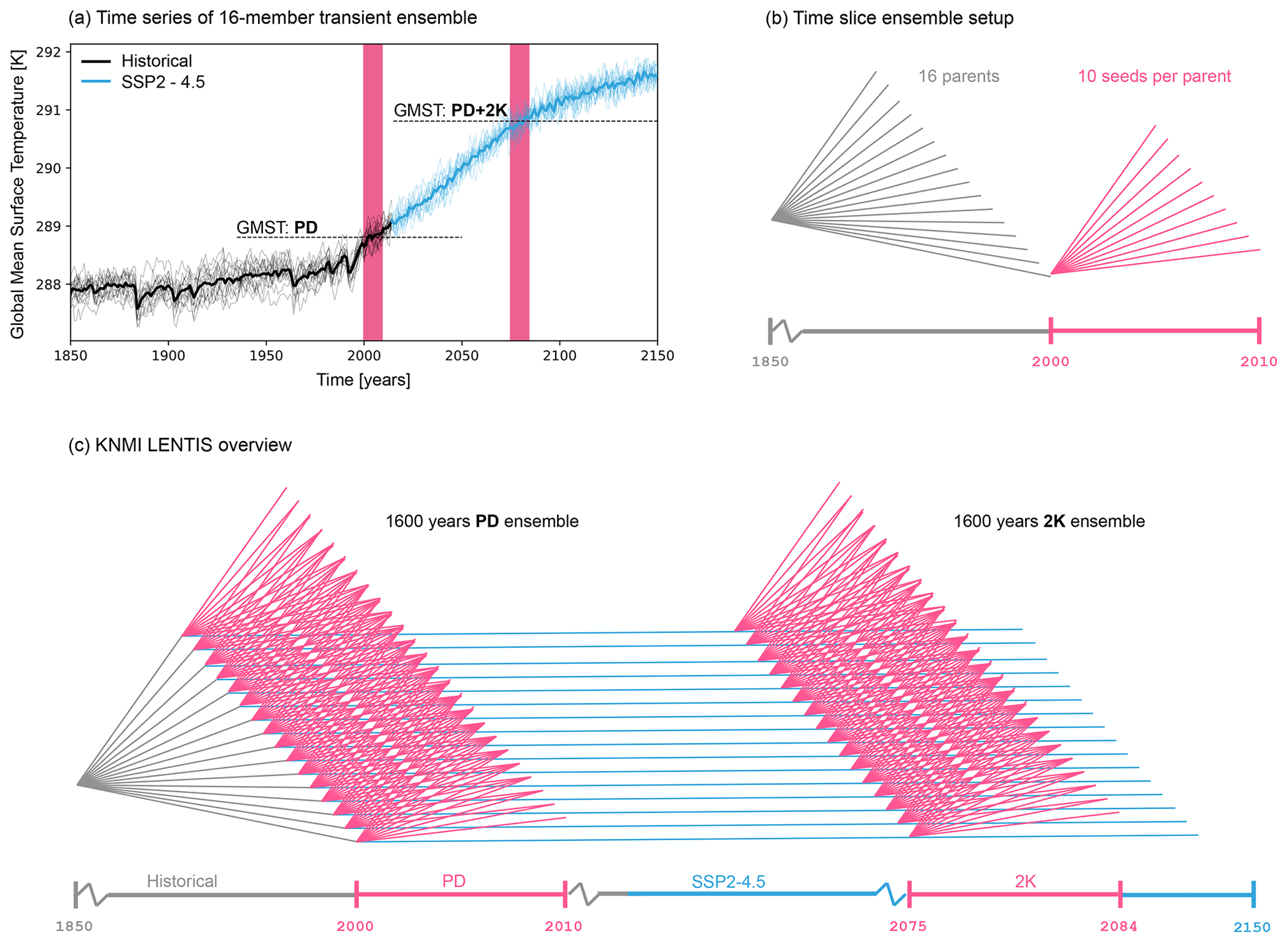
Figure 1 Overview of KNMI–LENTIS setup. (a) Global mean surface temperature (GMST) of the 16 ECE3p5 ensemble members forced with CMIP6 historical and SSP2-4.5 forcing. Pink shading shows the two time slices in KNMI–LENTIS. (b) Part of the time slice setup. From each of the 16 parent runs (grey), 10 KNMI–LENTIS simulations (pink) are branched using unique seeds to make a micro-perturbation in the atmospheric initial conditions. (c) The full ensemble consists of two time slices of 10 years with 1600 years of data each: the present day (PD) and present day +2 K global warming (2 K). The parents are visualized by the grey (historical) and blue (SSP2-4.5) lines. The KNMI–LENTIS simulations are visualized by the pink lines.

3 Limitations

In this section, we evaluate and discuss several aspects of the ensemble that are important for users to consider. We quantify the ensemble temperature difference between the present-day time slice and the +2 K time slice for different seasons and for several subsections of the world. We discuss the magnitude of the near-surface temperature biases in the model by making a comparison with ERA5 reanalysis data (Hersbach et al., 2020). Further, we discuss the validity of two critical assumptions:

1. Within a time slice, the 10-year segments are too short to show a significant forced climate change signal.

2. The ensemble size, 1600 years for both time slices, is sufficient to sample the full distribution of climate variability.

If true, this means that a single time slice can be used to investigate internal or natural climate variability at a given climatic state and that any differences between the two time slices can be attributed to forced climate change. Finally, we comment on the micro- and macro-initialization method and the legacy effect of a common parent on variability.

3.1 Temperature difference between the time slices

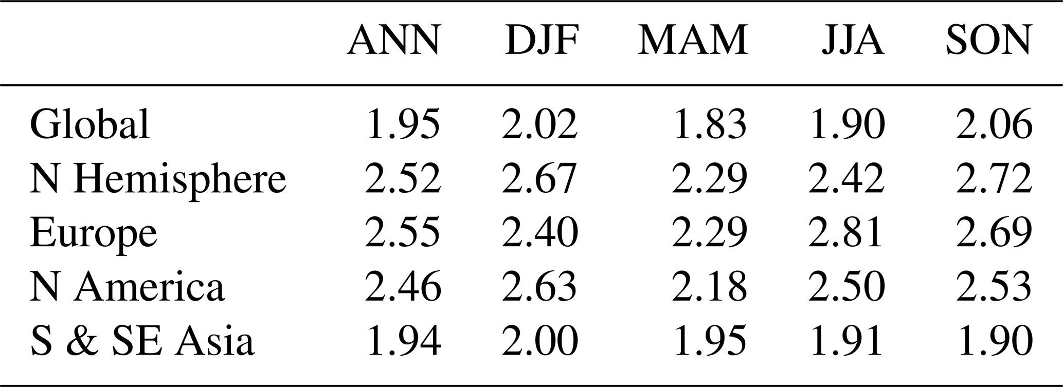
The 2 K time slice is designed to be 2 K warmer than the GMST of the present-day time slice, as detailed in Sect. 2.2. Here we quantify the ensemble spread of the surface temperature difference (ΔT_2 m) between the two time slices. The annual global mean ΔT_2 m is close to the GMST+2 K target: 1.95 K on average (Table 1). The spread in GMST is shown in Fig. 3a and c. Given that global climate change has specific local and regional imprints, the temperature difference is dependent on season and region. The 2 K time slice shows enhanced warming in the Northern Hemisphere, Europe, and North America. The South and Southeast Asia region is closer to the global value (Table 1).

Table 1 Temperature difference between the time slices. Ensemble mean of the near-surface air temperature difference (K) between the 2 K time slice and the PD time slice. The regions used to compute Europe, North America, and South and Southeast Asia means are shown in Fig. 2.

3.2 Quantification of model bias

The re-tuned EC-Earth3 ECE3p5 version has a known warm bias in the Southern Hemisphere (Sect. 2.1). In this section we quantify the magnitude of this bias and evaluate its spatial and temporal properties. The near-surface temperature of the present-day time slice of the ensemble is compared to ERA5 (Hersbach et al., 2020). We have chosen the World Meteorological Organization (WMO)-defined Climatological Standard Normals reference period 1991–2020 to have sufficient present-day climate variability to compare with. The ERA5 data are re-gridded to the coarser EC-Earth grid using nearest-neighbour interpolation.

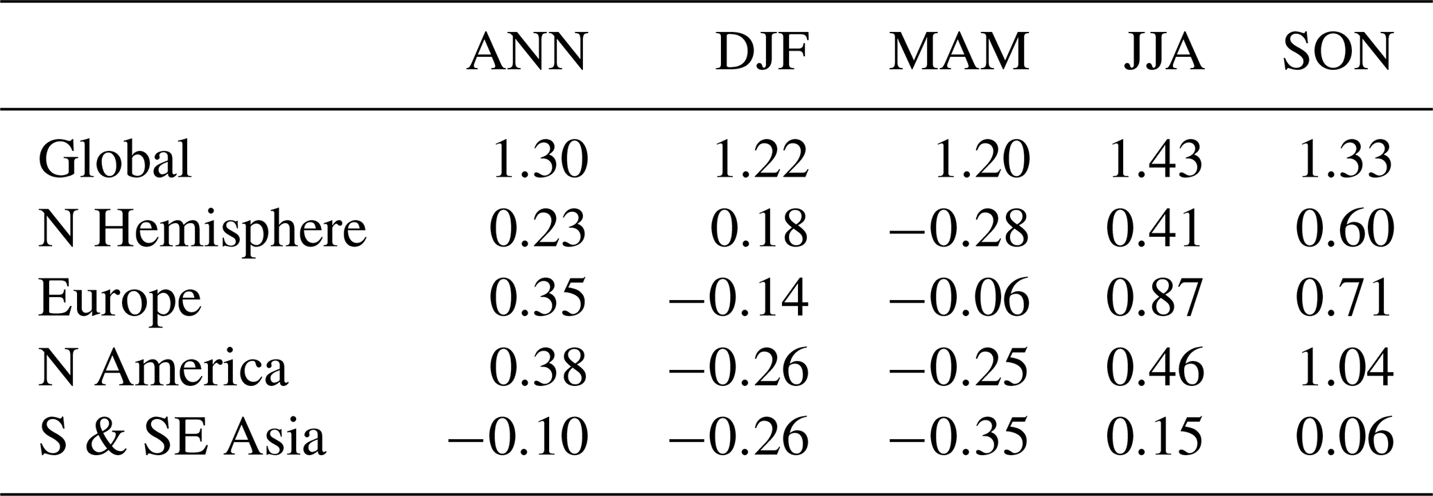
The global annual mean surface temperature bias in the PD time slice of KNMI–LENTIS with respect to ERA5 is 1.30 K (Table 2). This is largely due to a strong warm bias in the Southern Ocean and over Antarctica (Fig. 2a). The temperature bias over land is generally smaller in magnitude and more often insignificant compared to the ocean bias. The near-surface temperatures in the North Atlantic Gyre and the North Pacific Gyre are significantly underestimated.

The integrated annual mean temperature bias of the Northern Hemisphere is 0.23 K, which is much smaller than the global bias (Table 2). Further, we see a stronger seasonal expression of the bias in the Northern Hemisphere, with a larger bias in the summer and autumn and a smaller bias in winter and spring. There are regional differences, with generally cold bias in mountainous regions with steep orography. In all cases in the Northern Hemisphere, the bias is much smaller than the global bias. See Fig. 2b–d and Table 2 for specifications for the regions of Europe, North America, and South and Southeast Asia.

This outcome is in line with the expectations of using the re-tuned ECE3p5 version, of which the global warm bias is larger than that of the EC-Earth3 version in Döscher et al. (2022) but much improved for the Northern Hemisphere. Future users of KNMI–LENTIS are advised to make in-depth comparisons with observational or reanalysis data, especially if their study focuses on ocean processes, on locations in the Southern Hemisphere, or on teleconnections involving both hemispheres.

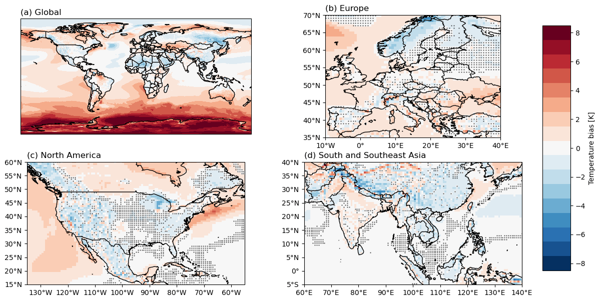
Figure 2 Model bias. Near-surface air temperature bias (K) for the annual-average ensemble mean of the KNMI–LENTIS present-day time slice [160 × (2000–2009)] compared to ERA5 (1991–2020), for the (a) global, (b) Europe, (c) North America, and (d) South and Southeast Asia regions. In panels (b)–(d) grid cells with a non-significant difference are dotted (p<0.01).

Table 2 Quantification of model bias w.r.t. ERA5 1991–2020. Ensemble mean of the near-surface air temperature bias (K) of the KNMI–LENTIS present-day 2000–2009 time slice w.r.t. ERA5 1991–2020. The regions for Europe, North America, and South and Southeast Asia are shown in Fig. 2.

3.3 Forced climate signal within a time slice

To quantify the size of the forced climate change signal relative to the interannual variability within the time slices (assumption 1), we investigate the linear trend of GMST (Fig. 3a, c). Both time slices have an interannual ensemble standard deviation of 0.17 K for the annual mean GMST value on average for the 10 time slice years. The linear trend over the 10-year simulation period is only slightly larger than this, at 0.20 K per 10 years for the PD ensemble and 0.22 K per 10 years in the 2 K ensemble (black error bars in Fig. 3a, c), approximately 1.25 times larger than the interannual ensemble standard deviation. At the global scale, we therefore conclude this assumption holds. Locally, or for other variables, forced trends may exceed the respective trends.

In Fig. 3b and d we show the ratio of the 10-year linear trend of near-surface temperature (TAS) and the ensemble standard deviation at the grid point level. Low values of this quantity are preferred. In most parts of the world, the value is smaller than 1, indicating a smaller forced trend than ensemble internal variability. We acknowledge that interannual variability is different for different variables. We therefore advise future users of KNMI–LENTIS to check the validity of assumption 1 on a case-by-case basis.

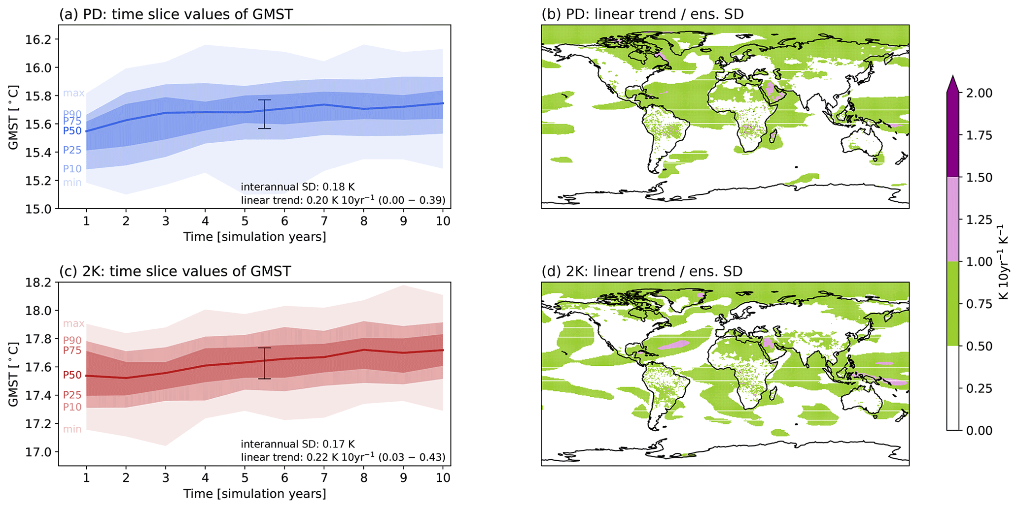
Figure 3 Quantification of assumption 1: size of forced trends within a time slice. (a, c) Ensemble spread of annual mean values of global mean surface temperature (GMST, shaded colours, percentile values denoted on the left). Ensemble interannual standard deviation and ensemble linear trend of GMST over 10 years shown in bottom-right corner, including the 80 % spread of this value for individual members. The black bar in the centre shows the size of this linear trend relative to the ensemble spread. (b, d) Global map of the ratio between the ensemble linear trend in near-surface temperature and the ensemble standard deviation in near-surface temperature. (a, b) The PD time slice. (c, d) The 2 K time slice.

3.4 Range of sampled internal variability

To test whether or not the full distribution of climate variability has been sampled in a 1600-year time slice (assumption 2), we investigate daily temperature variability at a single grid point (52.3^∘ N, 4.9^∘ E; nearest point to De Bilt, the Netherlands). We cannot test how different the distribution would be in a second set of 1600 years. Therefore we investigate differences between two halves of the PD ensemble, each of 800 simulation years. The shape of the distribution in Fig. 4a shows two peaks, which is a known phenomenon in the Netherlands due to the fairly rapid transition between the summer and winter season. The distributions of all daily temperature values in the two smaller ensembles are indistinguishable from each other, suggesting that variability has been adequately sampled in these half ensembles (see solid blue line and dotted green line in Fig. 4a and b). Sampling adequately in the tail of the distribution, e.g. for the warmest day of the year, requires larger sampling sizes. However, also here the two halves of the PD ensemble are statistically similar (Fig. 4b, differences between the generalized extreme value (GEV)-fitted distributions are well within the associated error bars). Comparing the PD distributions to the distribution of the 2 K ensemble, we note that forced climate change significantly impacts the shape of the distribution. We also note that variability beyond the scope of the climate model (e.g. at scales smaller or larger than resolved, missing processes) is not captured by these ensembles.

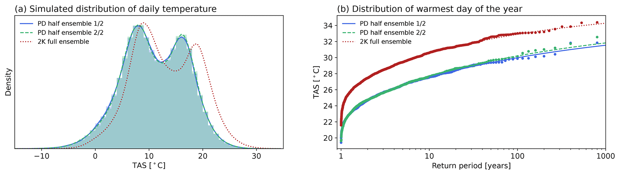
Figure 4 Quantification of assumption 2: sampling internal variability within a time slice. (a) Distribution of daily 2 m temperature (TAS) data at 52.3^∘ N, 4.9^∘ E, in two halves of the PD ensemble (blue and green shading and lines, each based on 800 years) and 2 K ensemble (dotted red line, based on 1600 years). (b) GEV fit distribution (lines) and modelled data (dots) value plot for the warmest day of the year, using the same colours as in (a).

3.5 Legacy of micro-perturbations in simulated variability

The way that the members of an ensemble are initialized impacts the climate variability of that ensemble in the initial stages. Specifically, when multiple initialization methods are combined, like the micro- and macro-perturbed initial conditions in the case of KNMI–LENTIS, there can be a too large degree of similarity at the beginning between similarly initialized members. Therefore, we need to assess the differences in variability between and among members of a common macro-perturbation (parent) at the beginning of the simulations and assess the time it takes to converge to a similar level of variability.

In KNMI–LENTIS, the initial conditions from a common parent of the ocean state are completely the same; only in the atmosphere state are there small differences due to the micro-perturbation. The legacy of information from the initial conditions has consequences for the estimated variability. This may show a spurious peak at this (early) year-1 value. The effect of the shared parent on variability differs per location and variable. We test this with a subset of parents for local near-surface temperature (TAS) variability in De Bilt, the Netherlands, and for El Niño–Southern Oscillation (ENSO) variability. The TAS variability in De Bilt seems to have lost the initial-condition information after around 20 simulation days (Fig. 5). For the ENSO signal it takes 2 or 3 years to lose the initial-condition information (Fig. 6).

An important goal of large-ensemble modelling is to be able to separate the part of the model outcome that can be attributed to a forced signal (climate change) from the part that comes from internal variability (climate variability). With this knowledge, we can reduce uncertainty in climate projections. There is a part of uncertainty that cannot be reduced, which is due to the chaotic nature of the climate system (i.e. irreducible uncertainty; see Hawkins et al., 2016; Marotzke, 2019; Singh et al., 2023). This can be sampled with the micro-perturbations. For the members of different macro-perturbations, the signal of common ancestry has to dissipate first. The above examples show how quickly the chaotic nature of the Earth system model takes over the initial-condition micro-perturbation. However, the speed of dispersion varies spatially and is variable dependent. We therefore advise future users to quantify this effect for their variables of interest and if necessary remove the first days/months/year of each simulation to ensure that estimates of variability do not suffer from this effect.

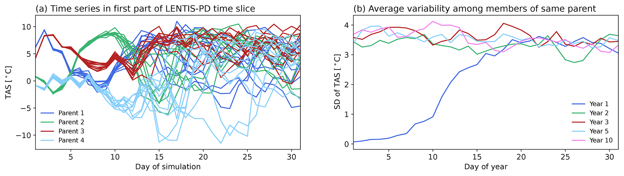
Figure 5 Test of influence of parent on variability: local TAS. (a) Time series, coloured by parent, of TAS at a grid point (52.3^∘ N, 4.1^∘ E) for the first 31 d of the simulations. (b) Time series of variability (estimated as the standard deviation of TAS of all members with a certain parent, then averaged over the parents) for different years in the time slice.

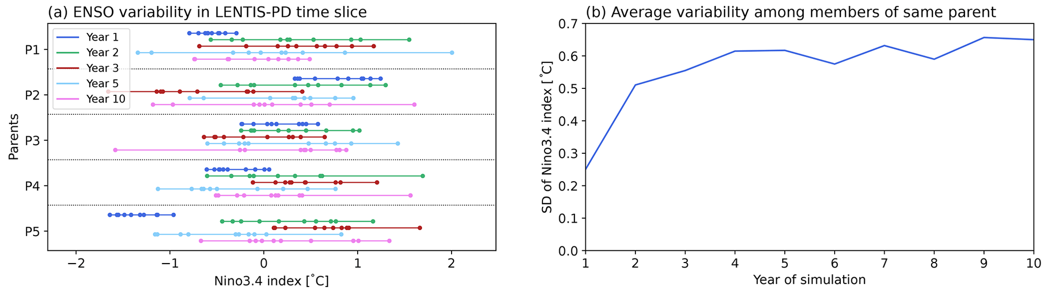
Figure 6 Test of influence of parent on variability: Niño 3.4. (a) Distribution of the annual mean Niño 3.4 index, separated by parent and simulation year. (b) Time series of variability (estimated as the standard deviation of Niño 3.4 of all members with a certain parent, then averaged over the parents) throughout the time slice.

4 Demonstration

In this section, we demonstrate the ensemble by giving examples of interesting cases. This ensemble has the unique feature of high-frequency output, allowing for detailed studies into extreme events. The surface water balance and surface energy balance variables are stored at 3-hourly intervals. Atmospheric variables (relative humidity, specific humidity, temperature, eastward wind, northward wind, omega) are saved daily on eight pressure levels (1000, 850, 700, 500, 250, 100, 50, 10 hPa). Additionally, a number of land, ocean, and atmosphere variables are stored monthly. The variables are post-processed and standardized to the CMIP6 convention. A full overview of the output variables can be found in the Supplement. More information on the variables and their output dimensions is accessible via the following search tool: https://clipc-services.ceda.ac.uk/dreq/mipVars.html (last access: 19 September 2022).

4.1 Climatological context of observed extreme events

Weather extremes usually take place at a point in time. This often raises questions about the climatological context of such an event and about the climate change aspects of similar events. KNMI–LENTIS can be used to determine, for example, the return interval of specific types of events. With this information we can infer the range of frequency and magnitude that can occur within the climate's variability and what the influence of climate change is on this (van Oldenborgh et al., 2021; van der Wiel et al., 2021).

The effect of the forced climate difference can be seen in other variables throughout the Earth system, since EC-Earth is a fully coupled climate model. Figure 7a–c highlight some extreme weather/climate events that have occurred in the recent past. The Greenland Ice Sheet (GrIS) has seen unprecedented melt events in recent years (e.g. http://nsidc.org/greenland-today/2021/08/large-melt-event-changes-the-story-of-2021/, last access: 3 October 2022). Figure 7a shows the simulated return intervals of July average snowmelt rates for a grid point in the eastern part of the Greenland Ice Sheet (72^∘ N, 30^∘ W). The higher return intervals in the 2 K time slice are due to a projected increase in future July melt event frequency.

The English Southern railway organization introduced speed restrictions during the 2022 heat wave in response to drying and shrinking of the clay soils, which made the train tracks prone to movement (e.g. https://www.networkrail.co.uk/stories/soil-moisture-deficit-on-the-railway/, last access: 3 October 2022). Figure 7b shows simulated surface air temperatures in July for a grid point in southern England (51^∘ N, 2^∘ W) against column-integrated soil moisture content for the PD and 2 K time slices. The upward–leftward shift of the scatter cloud indicates more co-occurrences of hot temperature–soil moisture deficit events in the warmer climate.

Finally, the World Meteorological Organization foresees “a strong chance of drier than average conditions in most parts of the Horn of Africa, making this the fifth consecutive failed rainy season” for the October–December 2022 season (e.g. https://www.africanews.com/2022/08/26/horn-of-africa-5th-consecutive-rainy-season-missed/, last access: 3 October 2022). Figure 7c shows the simulated seasonal cycle of precipitation at a grid point in the Horn of Africa (8^∘ N, 48^∘ E). In contrast to the news item, the simulated warmer climate appears to become generally wetter, with shifts in the start and intensity of the rain season. However, further analysis is required to draw conclusions on the occurrence of droughts.

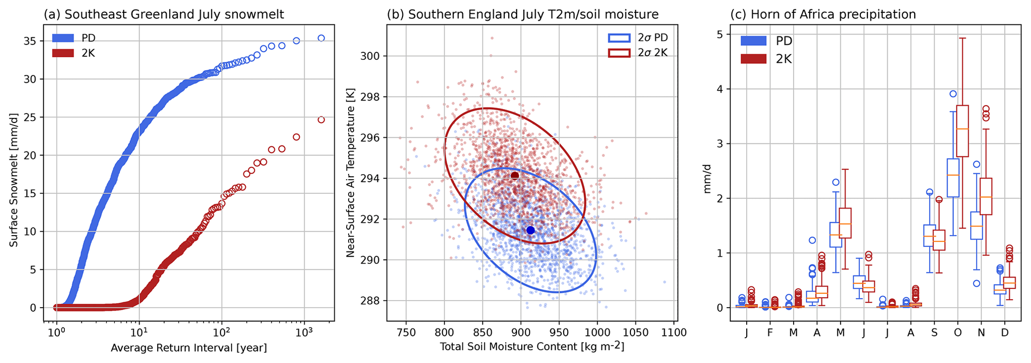
Figure 7 Ensemble climatology examples. For PD in blue and 2 K in red: (a) return interval in years of surface snowmelt rates at the eastern Greenland Ice Sheet grid point (72^∘ N, −30^∘ E); (b) scatter plot of total column-integrated soil moisture content and near-surface temperature at the southern England grid point (51^∘ N, −2^∘ E) with the cloud mean as a dot and 2 standard deviations in the ellipse; and (c) annual cycle of precipitation at the Horn of Africa grid point (8^∘ N, 48^∘ E). In (c), boxplots for the ensemble spread are defined as follows: box, first quartile–median–third quartile (interquartile range (IQR)); bottom whisker, −1.5 × IQR – first quartile; top whisker, third quartile – +1.5 × IQR; outliers, values outside of these limits.

4.2 Added value for extreme-meteorological-event research

Grey and blacks swans are terms for the types of extreme events that are as yet unobserved or cannot even have been anticipated, respectively (Watkins, 2013; Aven and Renn, 2015). These types of events by definition have no evidence in historical observations. Robust statistical analyses are often not possible due to their sparsity, not even with large-ensemble data. A recently developed technique into swan-type events is using storylines (Shepherd et al., 2018; Lloyd and Shepherd, 2021; Sillmann et al., 2021). By composing a storyline, the extreme event can be understood in terms of its spatial and temporal meteorological context. This can also help to gain understanding of such events in a different climate. KNMI–LENTIS provides a physically coherent set of simulations that allows for a storyline type of research into possible extreme meteorological events in the present day and in a 2 K warmer climate (van der Wiel et al., 2021).

In this example we identify the hottest day in De Bilt (52.3^∘ N, 4.9^∘ E), the Netherlands, in the PD time slice and its meteorological circumstances. The daily maximum near-surface air temperature reaches 39 ^∘C on this day. The hottest day to date in the observed records at the KNMI was measured on 25 July 2019, with a peak temperature of 37.5 ^∘C (https://www.knmi.nl/over-het-knmi/nieuws/warmste-dag-van-het-jaar-nu-4-c-warmer-dan-rond-1900, last access: 4 October 2022), demonstrating that the ensemble can indeed be used to study events beyond the observed record. Figure 8a shows very high maximum temperatures in a large area of western and central Europe and across the Mediterranean. The physical drivers of such an extreme event can be both large-scale warm air advection and local land–atmosphere processes. The evolution of surface energy balance components in De Bilt (Fig. 8b) does not suggest that local land–atmosphere processes are a main contributor to this heat event. The sea level pressure field over the Northern Hemisphere points to advection of hot air from the south (Fig. 8c). A small low-pressure system west of the British Isles seems important in directing the flow northwards. We note that temperatures in northern America are anomalously high as well (not shown). Further analysis is needed to assess whether the extremely hot weather is related to the specific configuration of high- and low-pressure systems that is seen in earlier studies in connection with simultaneously occurring heat waves in the Northern Hemisphere (Kornhuber et al., 2019).

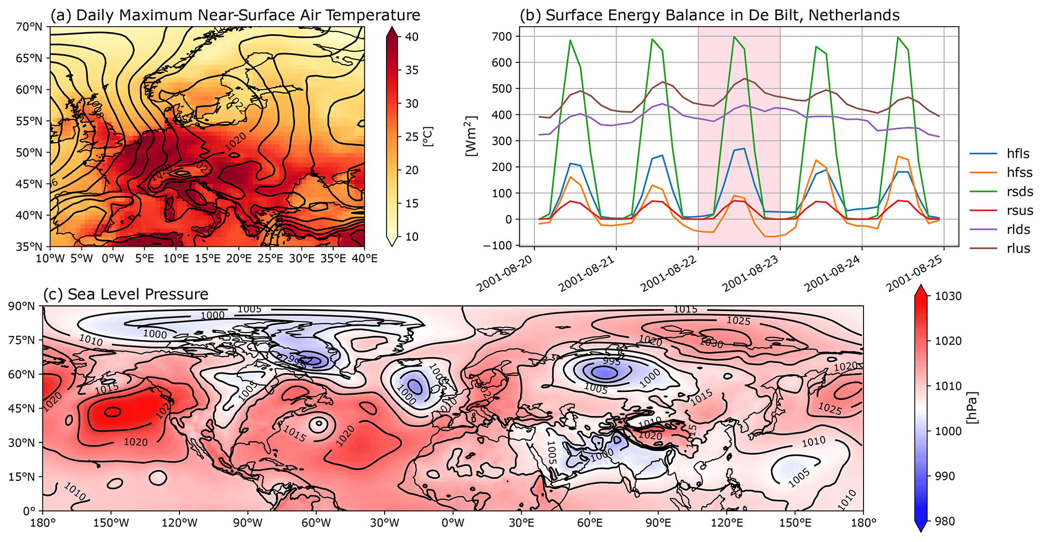
Figure 8 Hottest day in De Bilt, the Netherlands, in the PD ensemble. (a) Europe maximum surface air temperature over Europe on the hottest day (colours) and sea level pressure (contours every 5 hPa). (b) Surface energy balance components in De Bilt, the Netherlands, during the days around the hottest day (pink shading) with the latent heat flux (hfls), sensible heat flux (hfss), downwelling shortwave radiation (rsds), upwelling shortwave radiation (rsus), downwelling longwave radiation (rlds), and upwelling longwave radiation (rlus). The date format is year-month-day. (c) Northern Hemisphere sea level pressure in colours and in contours every 5 hPa.

4.3 Added value for compound-event research

The multivariate nature of compound events, events where combinations of climate drivers and/or hazards contribute to societal or environmental risk (Zscheischler et al., 2018), requires a bottom-up approach in which all data are physically consistent. Output from climate models is by definition physically consistent, though when bias corrections or statistical extrapolations are applied, this consistency may be broken (i.e. broken consistency between variables or lost consistency in time due to, for example, a water budget that is no longer closed). Time slice large ensembles are very suitable for the analysis of rare or extreme compound events (e.g. Kelder et al., 2022) owing to the physical consistency of the data and the explicitly resolved extreme events due to the size of the ensemble. In this section we demonstrate this using a case study on extreme wheat yield loss in France.

The 2016 winter-wheat harvest in France was exceptionally low (28 % lower than the expected value), and Ben-Ari et al. (2018) showed that this was caused by the “compound interaction between temperature in the late autumn/early winter and precipitation in the spring”. The year 2016 was unique in its combination of low exposure to cold days in autumn (“vernalizing days”, days with maximum temperatures between 0 and 10 ^∘C) followed by wet spring conditions (high precipitation). The historic record, here shown through ERA5 reanalysis data (Hersbach et al., 2020; Bell et al., 2021), shows how exceptional the year 2016 was in terms of these variables and especially in terms of their multivariate combination (Fig. 9).

The KNMI–LENTIS PD ensemble provides many more samples of winter-wheat growing conditions (1440 simulated seasons) than the observed historical record. The simulated data include some seasons with similar conditions to or even more extreme compounding conditions than the 2016 observed event (Fig. 9). This provides an opportunity to better understand the relationship between the governing variables and to investigate (remote) drivers of compounding conditions. Note that biases in the simulated data (here we find the model has a low bias in the number of vernalizing days) can impact estimates of event likelihood and process understanding.

This case study highlights the strength of time slice large ensembles in compound-event research. Also for other types of compound events (preconditioned events, multivariate events, temporally compounding events, and spatially compounding events; Zscheischler et al., 2020), large-ensemble data can help to, for example, quantify event likelihood and identify drivers and modulators of events (Bevacqua et al., 2021).

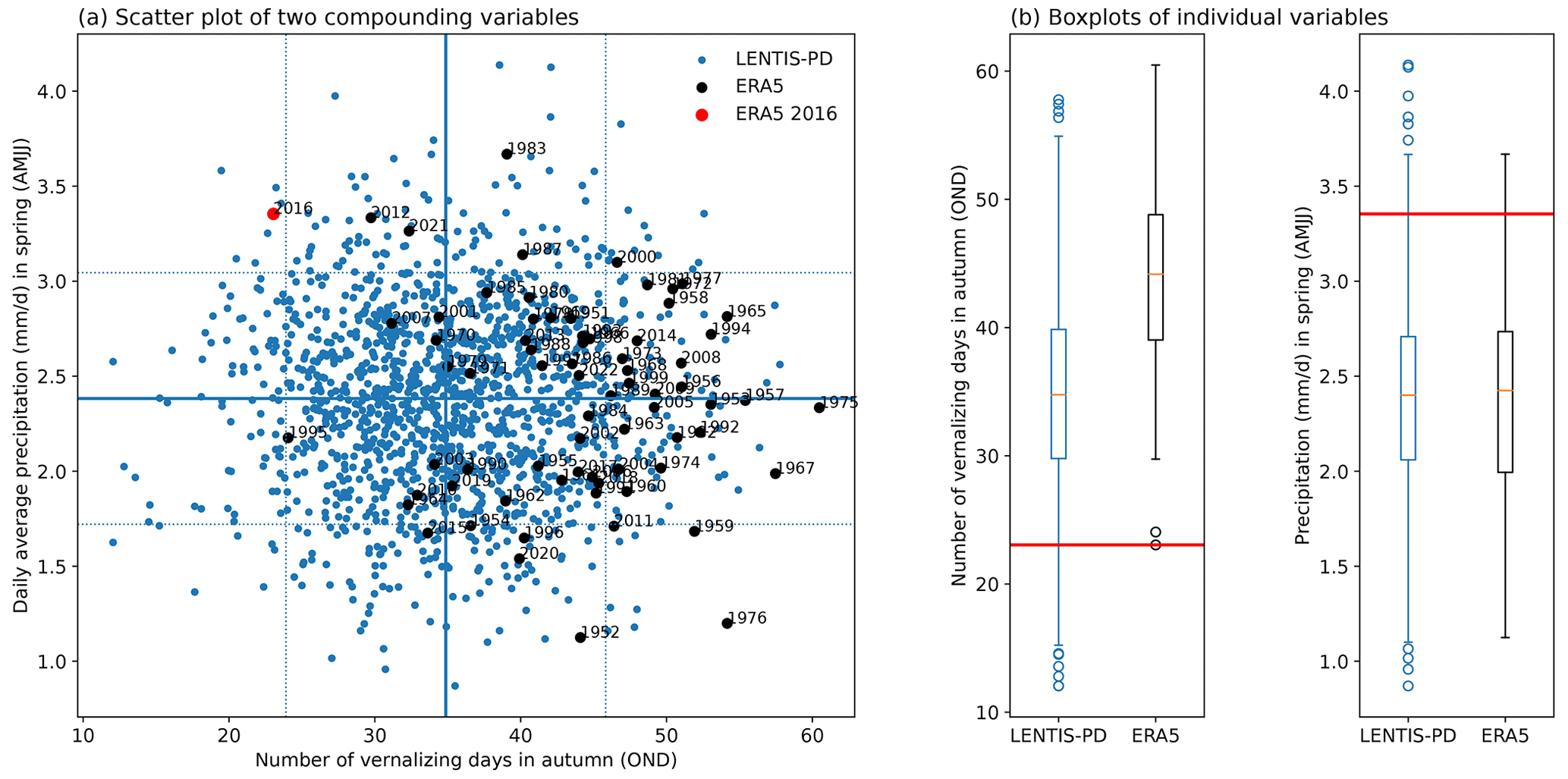
Figure 9 Example compound-event research. Analysis of meteorological circumstances that lead to extreme wheat yield loss in France after Ben-Ari et al. (2018). Presented values are the area average of the northern part of France (47–50^∘ N, 0–7^∘ E). (a) Scatter plot of number of vernalizing days in autumn (October–December) versus daily average precipitation in spring of the next year (April–July). Large black dots are ERA5 values (1950–2021), where 2016 is marked as a red dot. Small blue dots are KNMI–LENTIS PD values; horizontal and vertical lines correspond to the average (solid lines) ±1 standard deviation (dotted lines). (b) Boxplots of the number of vernalizing days and the daily average precipitation for both KNMI–LENTIS PD and ERA5.

4.4 Added value for climate-impact modelling

Climate science, apart from aiming to improve our scientific understanding of the physical Earth system, also aims to inform society and policy-makers of (future) risks caused by adverse weather. It is during extreme events that such risks are highest. However, extreme weather events (e.g. the hottest or wettest days) do not necessarily link 1-to-1 to extreme impact events (highest heat stress or biggest floods, e.g. van der Wiel et al., 2020). This is due to the complex non-linear relationships between weather and impacts. In this section we demonstrate this phenomenon and show that an approach of “ensemble climate-impact modelling”, as for example proposed by van der Wiel et al. (2020), enhances our understanding of the weather–impact relationship and improves estimates of (changing) societal risk.

For this case study, we simulate electricity production from solar radiation (photovoltaics, PV) with a relatively simple model that considers incoming solar radiation, near-surface temperatures, and near-surface wind speeds (Jerez et al., 2015; van der Wiel et al., 2019b). We use daily data at a single grid point in the Netherlands (De Bilt; 52.3^∘ N, 4.9^∘ E). Higher values of incoming radiation in summer (sunnier conditions and relatively long daylight hours) lead to higher values of PV generation, but the heating of solar cells negatively impacts generation (heating mostly related to high temperatures, some cooling provided by wind). We computed PV potential for all days in the KNMI–LENTIS PD ensemble (1600 years, $>\mathrm{0.5}\times {\mathrm{10}}^{\mathrm{6}}$ d). Here, we investigate the relationship between meteorological variables and PV potential, as well as the timing of extreme production days.

As expected, PV potential is strongly related to incoming solar radiation (Fig. 10a). The histogram shows a cluster for both DJF and JJA, indicating that solar cells work more efficiently in winter. This is due to differences in solar cell heating and daylight hours: for 100 W m⁻² incoming solar radiation, the PV potential in DJF is approximately 27 %, whereas in JJA it is approximately 18 %. On the other hand, the large seasonal difference in incoming radiation at this latitude makes summers about 5 times more productive in terms of PV (Fig. 10b). Therefore, extreme production events, i.e. days with extremely high PV potential, are expected to occur in late spring–early summer. Indeed the annual maxima of PV potential occur in early JJA, and they do not coincide with the annual maxima of incoming solar radiation (Fig. 10b), which occur later.

This case study highlights some of the possibilities of ensemble climate-impact modelling. Though extreme PV production days are not likely to put society at risk, the (temporal) disconnect between weather extremes on the one hand and impact extremes on the other hand is obvious. As shown in earlier sections, large-ensemble climate modelling can considerably contribute towards understanding events in the tail of the distribution. This is true not only for meteorological extremes (e.g. Sect. 4.2) but equally so for climate-impact extremes that are more closely related to possible natural or societal impacts/risk.

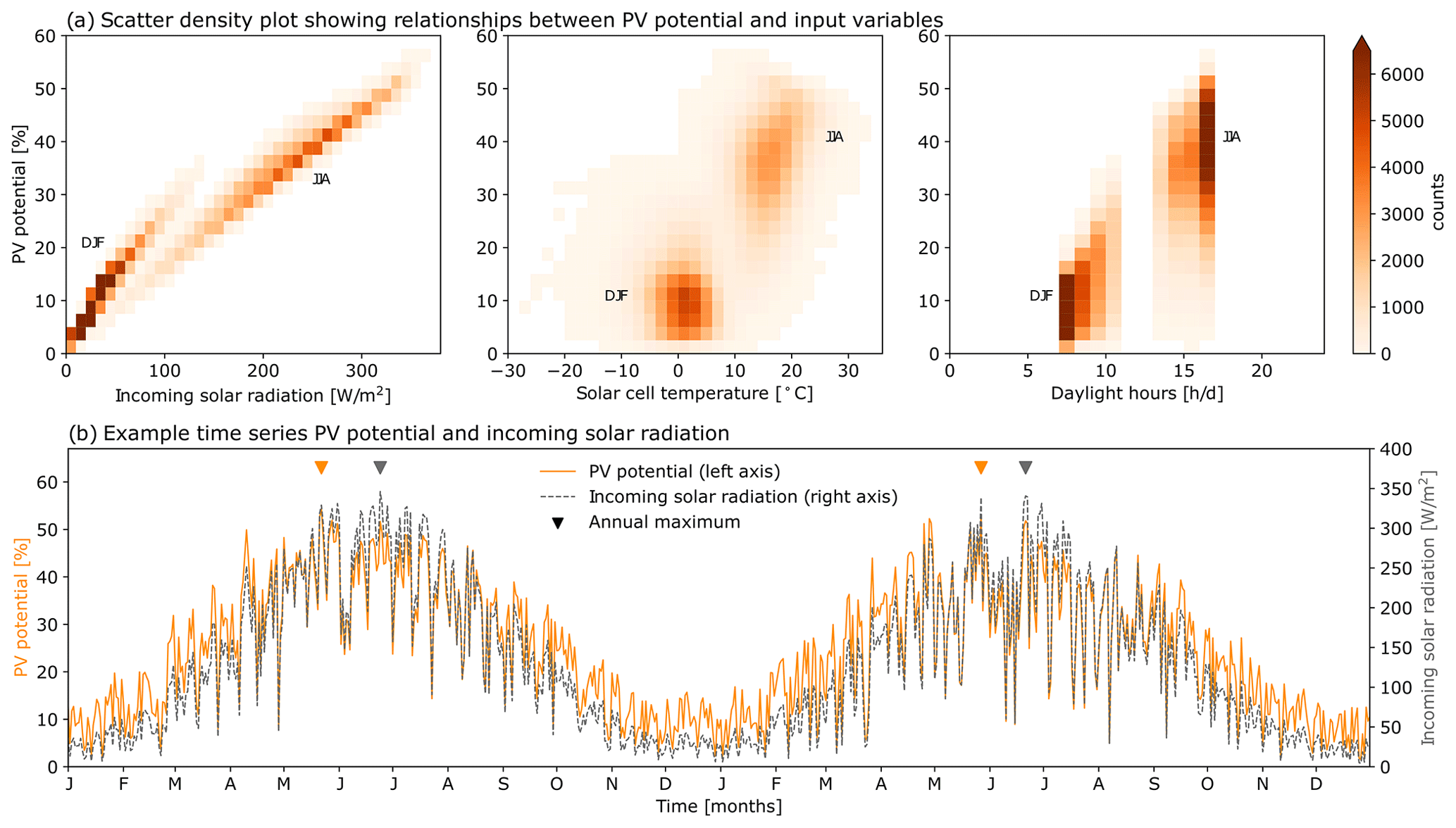
Figure 10 Example ensemble climate-impact modelling. (a) Scatter density plots showing the relationships between photovoltaics (PV) potential and other variables in DJF and JJA. From left to right: incoming solar radiation, solar cell temperature, and daylight hours. (b) Example time series of PV potential and incoming solar radiation. Triangles at the top show timing of annual maxima.

5 Conclusions

We have presented the KNMI Large Ensemble Time Slice (KNMI–LENTIS): a new large ensemble produced with the re-tuned version of the global climate model EC-Earth3. The time slice approach is different from the more traditional transient ensembles available from other institutions. Its advantage is that the signals of natural variability and climate change are not mixed due to our assumption that the forced change in a slice is small. Therefore, the variability we see in a time slice is only natural variability at a given GMST level and does not include a climate change signal. This renders our large ensemble specifically suitable to studying climate variability and changes therein between the present-day climate and a warmer future climate. Furthermore, the large ensemble is particularly geared towards research into the land–atmosphere interface, with 3-hourly output of the surface water balance and surface energy balance variables. ”two orders of magnitude” The ensemble consists of two distinct time slices: a present-day time slice and a +2 K warmer future time slice relative to the present day. The present-day time slice is represented by the years 2000–2009 and forced with CMIP6 historical forcing. The +2 K time slice is represented by the years 2075–2084 and forced with CMIP6 SSP2-4.5 forcing. Each time slice consists of 1600 simulated model years in 160 segments of 10 years.

The initial conditions for the ensemble members are generated with a combination of micro- and macro-perturbations. We have quantified the assumptions underlying the setup, which are that the time slice simulation length is small enough for a forced climate change signal to be minor in most cases and for the ensemble size to be sufficient to sample the full distribution of climate variability. We have provided examples of how this ensemble can be used to demonstrate its added value for extreme- and compound-event research and for climate-impact modelling. The model and thus our simulations have a considerable warm bias in the Southern Ocean and over Antarctica. Future users of KNMI–LENTIS are advised to make in-depth comparisons with observational or reanalysis data, especially when their studies focus on ocean processes, on locations in the Southern Hemisphere, or on teleconnections involving both hemispheres.

Appendix A: Ensemble label and CMIP6 variant label of KNMI–LENTIS simulations

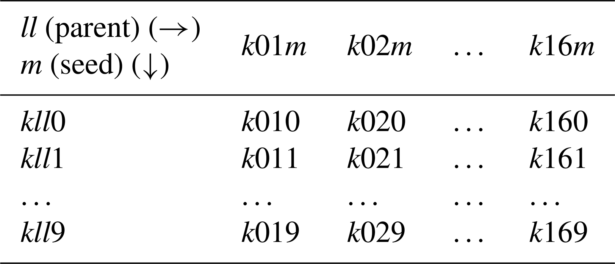
All ensemble simulations have a unique name that reflects the start year and forcing, the parent, and the seed (Table A1). The start year is noted in the first digit of the KNMI–LENTIS simulation name: “h” for the PD time slice and “s” for the 2 K time slice. The parent is reflected in the second and third digit. The seed is reflected in the fourth digit.

Further, all KNMI–LENTIS simulations are labelled per the CMIP6 convention of variant labelling. A variant label is made from four components: the realization index r, the initialization index i, the physics index p, and the forcing index f. Further details on CMIP6 variant labelling be found in the “CMIP6 Participation Guidance for Modelers”: https://pcmdi.llnl.gov/CMIP6/Guide/modelers.html (last access: 20 September 2022).

In the KNMI–LENTIS simulations, the forcing is reflected in the first digit of the realization index r of the variant label. For the historical simulations, numbers in the range r1000–r1999 have been reserved. For SSP2-4.5, numbers in the range r5000–r5999 have been reserved. The parent is reflected in the second and third digit of the realization index r of the variant label (rX01X–rX16X). The seed is reflected in the fourth digit of the realization index r: (rXXX0–rXXX9), The seed is also reflected in the initialization index i of the variant label (i0–i9), so this is double information. The physics index p5 has been reserved for the ECE3p5 version, so all KNMI–LENTIS simulations have the p5 label. The forcing index f of the variant label is kept at 1 for all KNMI–LENTIS simulations. As an example, variant label r5119i9p5f1 refers to the 2 K time slice with parent 11 and randomizing seed number 9. The physics index is 5, meaning the run is done with the ECE3p5 version of EC-Earth3.

Table A1 Naming convention of LENTIS members. The simulations are named with a four-character name: kllm. The term “k” is a placeholder to denote the start year. Options are h for 2000-historical and s for 2075-SSP2-4.5. The term “ll” is a placeholder to denote the parent. Parents run from 01 to 16, from whose full transient simulation the initial conditions are taken. The term “m” is a placeholder to denote the seed. Seeds run from 0 to 9, corresponding to the randomizing seed of the micro-perturbation.