Breakups are complicated: an efficient representation of collisional breakup in the superdroplet method

A key constraint of particle-based methods for modeling cloud microphysics is the conservation of total particle number, which is required for computational tractability. The process of collisional breakup poses a particular challenge to this framework, as breakup events often produce many droplet fragments of varying sizes, which would require creating new particles in the system. This work introduces a representation of collisional breakup in the so-called “superdroplet” method which conserves the total number of superdroplets in the system. This representation extends an existing stochastic collisional-coalescence scheme and samples from a fragment size distribution in an additional Monte Carlo step. This method is demonstrated in a set of idealized box model and single-column warm-rain simulations. We further discuss the effects of the breakup dynamic and fragment size distribution on the particle size distribution, hydrometeor population, and microphysical process rates. Box model experiments serve to characterize the impacts of properties such as coalescence efficiency and fragmentation function on the relative roles of collisional breakup and coalescence. The results demonstrate that this representation of collisional breakup can produce a stationary particle size distribution, in which breakup and coalescence rates are approximately equal, and that it recovers expected behavior such as a reduction in precipitate-sized particles in the column model. The breakup algorithm presented here contributes to an open-source pythonic implementation of the superdroplet method, PySDM, which will facilitate future research using particle-based microphysics.

1 Introduction

The superdroplet method (SDM) for cloud microphysics is a high-fidelity particle-based (Lagrangian) representation of aerosols and hydrometeors that offers notable advantages over traditional bulk and bin microphysics schemes. Particle-based methods were initially used in atmospheric simulations to represent ice nucleation (Paoli et al., 2004; Jensen and Pfister, 2004; Shirgaonkar and Lele, 2006; Sölch and Kärcher, 2010) and were later extended to study aerosol indirect effects with a superdroplet approach (Andrejczuk et al., 2008) in which each superdroplet represents a multiplicity of modeled particles with identical attributes, such as size and chemical properties. Later, the SDM was extended to include a stochastic representation of collisional coalescence (Shima et al., 2009; Riechelmann et al., 2012) and ice-phase processes (Shima et al., 2020), making the SDM a nearly complete Monte Carlo representation of cloud microphysics. The burgeoning field of particle-based cloud microphysics uses SDM implementations in large-eddy simulations (LESs) to understand microphysical processes that are underresolved in traditional bulk and bin methods (e.g., Chandrakar et al., 2021; Andrejczuk et al., 2010; Morrison et al., 2019; Dziekan et al., 2019; Grabowski, 2020; Hoffmann, 2017). Furthermore, a growing literature of machine learning in microphysics utilizes the SDM as a source of high-fidelity training data from which to “learn” microphysical tendencies and properties (Bieli et al., 2022; Seifert and Rasp, 2020). However, without a complete representation of microphysical processes in the SDM, its predictive and benchmarking power for cloud feedbacks is limited.

Many implementations of the SDM do not include the process of collisional breakup of droplets. Not only is collisional breakup a highly uncertain process in existing bin and bulk parameterizations (Morrison et al., 2020; Grabowski et al., 2019), but these uncertainties have been found to impact rain rates and other macroscale quantities in bin microphysics studies (Seifert et al., 2005). Studying collisional breakup in the SDM is not straightforward, as it requires balancing computational complexity within a mass-conserving numerical model that respects the physics of the process. Notably, a single breakup event is likely to produce fragments of multiple different sizes. A literal representation of all fragments in the SDM would require the creation of new superdroplet tracers for each new droplet size resulting from breakup, which can lead to an explosive growth of superdroplet quantity and dramatically inhibit performance of the SDM. Another option that reduces the computational burden of new superdroplets involves creating and then selectively merging superdroplets, as in Bringi et al. (2020). While both options respect mass conservation and the physics of superdroplet breakup, a scalable adaption of the SDM for parallel applications such as LES requires strict conservation of the total number of superdroplets. This work proposes a superdroplet-conserving SDM algorithm for the process of collisional breakup, conceptually similar to the mass-flux algorithm of Kotalczyk et al. (2017), using a Monte Carlo step that samples from a fragment size distribution.

This superdroplet-conserving breakup implementation draws inspiration from an analogous “superparticle” representation of phytoplankton (Jokulsdottir and Archer, 2016): individual phytoplankton aggregates spontaneously break uniformly into a number of fragments determined by a power law probability distribution. We apply a similar spontaneous breakup principle to an intermediate coalesced state resulting from the collision of two droplets. (While spontaneous breakup of liquid water droplets has also been investigated (Kamra et al., 1991), it has not been observed in in situ studies of droplet collisions (Testik and Rahman, 2017) and is not included in this version of the SDM.) The presented collisional-breakup algorithm utilizes empirical collection efficiencies (such as Schlottke et al., 2010; Beard and Ochs, 1995; Berry, 1967) to determine whether a colliding droplet pair is likely to break up, and the algorithm then samples from a corresponding empirical fragment size distribution (such as Low and List, 1982; Schlottke et al., 2010; Beard and Ochs, 1995; McFarquhar, 2004) to determine the properties of the resulting fragmented superdroplet. Breakup parameterizations are typically very complex and aim to summarize multiple physical mechanisms of breakup. This work addresses how the proposed SDM breakup algorithm samples from such complex fragment size distributions but leaves the evaluation and analysis of these empirical distributions to future work.

The contents of this paper proceed as follows: Sect. 2 begins with a conceptual description of the proposed breakup algorithm, followed by a mathematical description of its implementation. Section 3 validates the implementation against analytical results in the literature and explores convergence with number of superdroplets. Section 4 then presents several idealized simulations including various parameterizations of collisional breakup to demonstrate the behavior of this implementation in the SDM. Section 5 concludes the discussion and poses additional scientific questions which may be within reach given this novel implementation.

2 Superdroplet-conserving collisional breakup

2.1 Conceptual description

Two colliding liquid hydrometeors in the atmosphere can break up via several physical pathways, including filament, sheet, and disk breakup (Barros et al., 2008). The colliding droplets, referred to as “parents”, typically lose mass to newly formed tiny “satellite” droplets that result from the collision, thereby resulting in several differently sized droplet fragments (see Fig. 1, left). As noted previously, computational scaling of the SDM relies on preserving the number of tracers in the system. In order to preserve the number of superdroplets in a binary collisional-breakup event, breakup is treated as a two-step process based on superdroplet-conserving coalescence (Fig. 1, right). First, the two superdroplets collide and coalesce: the superdroplet of higher multiplicity acts as a “donor” by donating mass and multiplicity while maintaining its attributes; the other superdroplet acts as a “receiver” by growing in mass and maintaining its multiplicity to form a “coalesced transition state”. This unstable coalesced transition state immediately breaks up into fragments of uniform size: the fragment size is selected sampling from a distribution of fragment sizes that encompasses both the remnants of the original parent droplets and the distribution of satellite fragments that can result from the collision. (Going forward, the term “fragment” will be used to describe all collisional-breakup products, both small satellite fragments and larger fragments that are nearer in size to the original colliding droplets.) The attributes and multiplicity of this fragmented receiver are updated, with multiplicity increasing and mass of the individual droplets represented by the superdroplet decreasing. Uniform fragmentation is required to maintain conservation of superdroplets. Furthermore, uniform fragmentation requires the assumption that all superparticle attributes are extensive quantities and undergo equipartitional splitting (not applicable, e.g., for insoluble aerosol constituents). The product of a collisional-breakup event is therefore two superdroplets: the donor maintains its attributes but donates multiplicity, and the fragmented receiver represents (uniform) fragments that result from the breakup event following a coalesced transition state. As in the original Monte Carlo step that determines whether a collision occurs, the fragment size is sampled at random from a fragment size distribution, which may depend on the properties of the colliding particles.

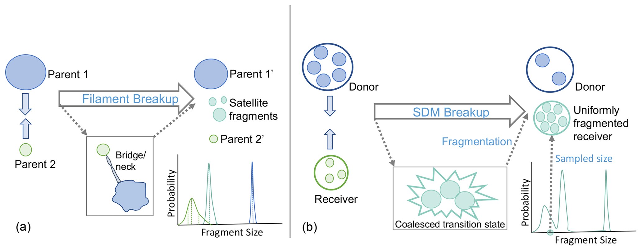
Figure 1 Conceptual view of a real filament breakup event (a) and the superdroplet-number-conserving SDM collisional-breakup dynamic described in this work (b). The real event involves collision between two parent droplets, which may form a neck bridging each other before fragmenting into several differently sized droplets. The resulting droplets consist of larger fragments derived from the initial colliding parents plus a set of small fragments known as “satellites”. Each of these groups forms a subdistribution in the overall fragmentation function, shown below the droplet schematics. The tracer-conserving SDM representation involves collision of two groups of droplets (each group represented as one superdroplet, a donor and receiver), which collide and coalescence into a transition state, which then fragments uniformly to a size sampled from the same fragmentation function as in the real case. The result of the SDM breakup is two superdroplets, or two groups of droplets, with one group corresponding to leftover donor droplets and the other group corresponding to a set of fragments whose size may correspond to the depleted parent droplet size or the satellite fragments, depending on the fragment size sampling step.

2.2 Mathematical description

The superdroplet-conserving method of collisional breakup is illustrated in Fig. 2 and formulated below using notation following work of Shima et al. (2009). A single superdroplet with label i has a position x_i(t) and extensive physical attributes a_i(t), such as droplet volume or mass (v_i(t),m_i(t)) or mass of solute (M_i(t)). (Note that in Shima et al.'s, 2009, notation, a_i(t) includes attributes such as droplet radius, whereas we only consider attributes which are linearly additive and extensive in the droplet size, such as volume or mass.) For simplicity, we will generally group all such extensive attributes together as a_i(t) but will specifically use the droplet mass m_i in computations of the transfer of extensive properties between superdroplets. Each superdroplet corresponds to a multiplicity ξ_i(t) of “real” droplets which exist in the same grid box and have identical such attributes.

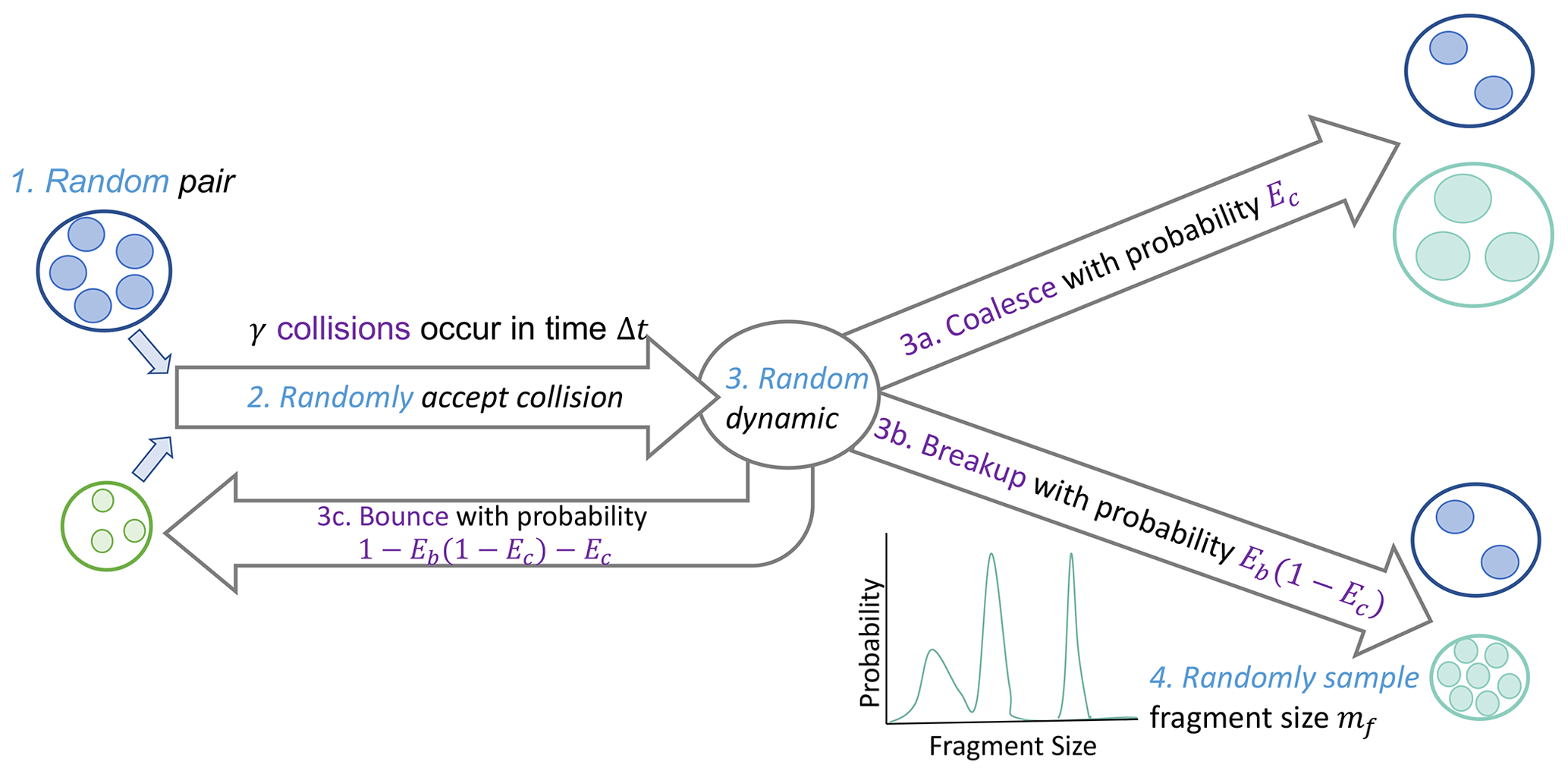
Figure 2 Diagram of the Monte Carlo decision pathway during a collision–coalescence–breakup event in the proposed algorithm.

The proposed breakup algorithm unifies the representation of collisional coalescence and breakup and builds on the original coalescence Monte Carlo steps in Shima et al. (2009). As in this original SDM, we begin by selecting pairs of superdroplets to consider collisions.

• 1.

  All superdroplets within a cell are randomly ordered in a list of non-overlapping pairs (j_α,k_α), where j and k are the superdroplet indices, and α refers to the pair index.

Next, we determine how many collisions, γ_α, occur for the pair α in the time step.

• 2.

  The probability of collision between droplets i and j is given by

  $$\begin{array}{}\text{(1)}& {\displaystyle }{P}_{i,j}=K_{i,j}\mathrm{\Delta }t,\end{array}$$

  where K_i,j is the rate of collisions based on the properties of droplets i and j, and Δt is the model time step. The scaled probability of collision $P_{\mathit{\alpha }}^{\left(\mathrm{s}\right)}$ for this pair α accounts for the multiplicities of the colliding superdroplets:

  $$\begin{array}{}\text{(2)}& {\displaystyle }{P}_{\mathit{\alpha }}^{\left(\mathrm{s}\right)}=max({\mathit{\xi }}_j,{\mathit{\xi }}_k)P_{\mathit{\alpha }}.\end{array}$$

  Only a subset $⌊n_{\mathrm{s}}/\mathrm{2}⌋$ of possible SD pairs are considered out of all possible superdroplet pairs at each time step. Therefore, the probability is further scaled up to form the corrected probability of collision:

  $$\begin{array}{}\text{(3)}& {\displaystyle }{p}_{\mathit{\alpha }}={\displaystyle \frac{n_{\mathrm{s}}(n_{\mathrm{s}}-\mathrm{1})}{\mathrm{2}}}/⌊{\displaystyle \frac{n_{\mathrm{s}}}{\mathrm{2}}}⌋P_{\mathit{\alpha }}^{\left(\mathrm{s}\right)}.\end{array}$$

  The number of collisions that occur in this time step, γ_α, is then determined in a Monte Carlo step based on p_α. Taking ${\mathit{\varphi }}_{\mathit{\alpha }}\in (\mathrm{0},\mathrm{1})$ to be a uniform random number,

  $$\begin{array}{}\text{(4)}& {\displaystyle }{\mathit{\gamma }}_{\mathit{\alpha }}=min(\lceil p_{\mathit{\alpha }}-{\mathit{\varphi }}_{\mathit{\alpha }}\rceil ,\lfloor {\mathit{\xi }}_{j_{\mathit{\alpha }}}/{\mathit{\xi }}_{k_{\mathit{\alpha }}}\rfloor ).\end{array}$$

  Here, we assumed the superdroplets are ordered such that ${\mathit{\xi }}_{j_{\mathit{\alpha }}}\ge {\mathit{\xi }}_{k_{\mathit{\alpha }}}$. If γ_α=0, then no collisions occur.

The collision rate is then γ_α collisions per grid box and per time step. Due to the constraint in Eq. (4) based on droplet multiplicity, some collisions which should occur probabilistically cannot if the donor superdroplet has insufficient multiplicity to collide p_α times. Therefore, a collision deficit p_α−γ_α may be tracked as a tool to assess whether the model time step is sufficiently small (elimination of the collision deficit is used for adaptive step size control in the SDM implementation used herein, Arabas et al., 2022).

In the original SDM, particles coalesce as long as γ_α>0, as the rate of collisions is taken to refer only to collisional coalescence. However, when we consider collisional breakup, an additional Monte Carlo step must be taken to determine whether the particles coalesce or break up. This is determined based on a coalescence efficiency (or collection efficiency) E_c, which generally depends on properties of the colliding particles such as their fall speed, mass, and surface tension. We additionally account for the fact that in some collisions, droplets may bounce off one another elastically by including an optional additional parameter for the breakup efficiency, E_b. This second Monte Carlo step is summarized as follows.

• 3.

  Compute the dynamic that occurs: coalescence, breakup, or bounce (nothing). A second uniform random number ${\mathit{\varphi }}_{\mathit{\alpha }}^{\prime }$ determines the outcome:

  $$\begin{array}{}\text{(5)}& \begin{array}{rl}& {\mathrm{dynamic}}_{\mathit{\alpha }}=\\ & \left\{\begin{array}{ll}\mathrm{coalescence},& {\mathit{\varphi }}_{\mathit{\alpha }}^{\prime }\le E_{\mathrm{c}}({\mathbf{a}}_j,{\mathbf{a}}_k)\\ \mathrm{breakup},& E_{\mathrm{c}}({\mathbf{a}}_j,{\mathbf{a}}_k)<{\mathit{\varphi }}_{\mathit{\alpha }}^{\prime }\le \\ & E_{\mathrm{b}}({\mathbf{a}}_j,{\mathbf{a}}_k)(\mathrm{1}-E_{\mathrm{c}}({\mathbf{a}}_j,{\mathbf{a}}_k\left)\right)+E_{\mathrm{c}}({\mathbf{a}}_j,{\mathbf{a}}_k)\\ \mathrm{bounce},& {\mathit{\varphi }}_{\mathit{\alpha }}^{\prime }>\\ & E_{\mathrm{b}}({\mathbf{a}}_j,{\mathbf{a}}_k)(\mathrm{1}-E_{\mathrm{c}}({\mathbf{a}}_j,{\mathbf{a}}_k\left)\right)+E_{\mathrm{c}}({\mathbf{a}}_j,{\mathbf{a}}_k).\end{array}\right.\end{array}\end{array}$$

Once the dynamic is determined, a fragment size is sampled if necessary.

• 4.

  Sample a fragment size m_f,α (mass) from a fragment size distribution, P_f,α, with cumulative distribution function (CDF) C_f,α(ϕ) that depends on the colliding particle attributes. A related variable, N_f,α, is taken to denote the number of fragments that would form in a collision between droplets of mass m_j and m_k: $N_{\mathrm{f},\mathit{\alpha }}=\frac{m_k+m_j}{m_{\mathrm{f},\mathit{\alpha }}}$.

Finally, updating of multiplicities and attributes proceeds based on the selected dynamic, number of collisions, and sampled fragment size (if applicable).

• (a)

  For coalescence.

  $$\begin{array}{}\text{(6)}& {\displaystyle }\left\{\begin{array}{l}{\mathit{\xi }}_j^{\prime }={\mathit{\xi }}_j-{\mathit{\gamma }}_{\mathit{\alpha }}{\mathit{\xi }}_k\\ {\mathbf{a}}_k^{\prime }={\mathbf{a}}_k+{\mathit{\gamma }}_{\mathit{\alpha }}{\mathbf{a}}_j\\ \mathrm{if}{\mathit{\xi }}_j^{\prime }=\mathrm{0},\mathrm{then}{\mathit{\xi }}_j^{\prime },{\mathit{\xi }}_k^{\prime }={\mathit{\xi }}_k/\mathrm{2},{\mathbf{a}}_j^{\prime }={\mathbf{a}}_k.\end{array}\right.\end{array}$$

  The coalescence rate is incremented by γ_αξ_k. The final step in updating multiplicities and attributes serves to conserve the number of superdroplets with nonzero multiplicity in the simulation in the event that all droplets within superdroplet j are depleted. Unlike in Shima et al. (2009), where superdroplet j is discarded, this approach sets properties of superdroplet j to be identical to k and sets both j and k to half of k's multiplicity to conserve mass.

• (b)

  For breakup.
  In some cases, only γ_jk≤γ_α breakups can occur for a given superdroplet pair without encountering negative multiplicities. We compute this maximum possible number of breakup steps and update the superdroplet properties using a recurrence relation (assuming γ_α>0), and we track a breakup deficit rate of γ_α−γ_jk. (Alternatively, one may perform substepping of the breakup event.) The particle attributes are updated such to be consistent with the result of several breakup steps with γ_α=1 occurring in sequence, always producing fragments of size m_f,α.

  $$\begin{array}{}\text{(7)}& {\displaystyle }& {\displaystyle }\left\{\begin{array}{l}{\mathit{\gamma }}_{jk}=\mathrm{0}\\ {\mathit{\xi }}_j^{\text{transfer}}=\mathrm{0},{\mathit{\xi }}_{j,\text{next}}^{\text{transfer}}={\mathit{\xi }}_k\\ {\mathit{\xi }}_k^{\text{new}}={\mathit{\xi }}_k,{\mathit{\xi }}_{k,\text{next}}^{\text{new}}={\mathit{\xi }}_k\left(\frac{m_j+m_k}{m_{\mathrm{f},\mathit{\alpha }}}\right)\\ \text{while}{\mathit{\gamma }}_{jk}<{\mathit{\gamma }}_{\mathit{\alpha }}\text{and}{\mathit{\xi }}_{j,\text{next}}^{\text{transfer}}\le {\mathit{\xi }}_j:\\ {\mathit{\xi }}_j^{\text{transfer}}={\mathit{\xi }}_{j,\text{next}}^{\text{transfer}}\\ {\mathit{\xi }}_k^{\text{new}}={\mathit{\xi }}_{k,\text{next}}^{\text{new}}\\ {\mathit{\gamma }}_{jk}={\mathit{\gamma }}_{jk}+\mathrm{1}\\ {\mathit{\xi }}_{j,\text{next}}^{\text{transfer}}={\mathit{\xi }}_{j,\text{next}}^{\text{transfer}}+{\mathit{\xi }}_{k,\text{next}}^{\text{new}}\\ {\mathit{\xi }}_{k,\text{next}}^{\text{new}}={\mathit{\xi }}_{k,\text{next}}^{\text{new}}\left(\frac{m_j}{m_{\mathrm{f},\mathit{\alpha }}}\right)+{\mathit{\xi }}_{k,\text{next}}^{\text{new}}\end{array}\right.\text{(8)}& {\displaystyle }& {\displaystyle }\left\{\begin{array}{l}{\mathit{\xi }}_j^{\prime }={\mathit{\xi }}_j-{\mathit{\xi }}_j^{\text{transfer}}\\ {\mathit{\xi }}_k^{\prime }={\mathit{\xi }}_k^{\text{new}}\\ {\mathbf{a}}_k^{\prime }=\frac{{\mathit{\xi }}_k{\mathbf{a}}_k+{\mathit{\xi }}_j^{\text{transfer}}{\mathbf{a}}_j}{{\mathit{\xi }}_k^{\text{new}}}\\ \text{if }{\mathit{\xi }}_j^{\prime }=\mathrm{0},\text{ then }{\mathit{\xi }}_j^{\prime },{\mathit{\xi }}_k^{\prime }={\mathit{\xi }}_k^{\text{new}}/\mathrm{2},{\mathbf{a}}_j^{\prime }={\mathbf{a}}_k^{\prime }\end{array}\right.\end{array}$$

  The breakup rate is incremented by γ_jkξ_k. The breakup deficit rate is incremented by (γ_α−γ_jk)ξ_k

• (c)

  For bounce.
  No update is made to droplet multiplicities or attributes, and only the collision counter is incremented.

2.3 Additional implementation details

This method of breakup allows for the splitting of a coalesced transition state into a non-integer number of fragments ($N_{\mathrm{f},\mathit{\alpha }}=\frac{m_k+m_j}{m_{\mathrm{f},\mathit{\alpha }}}$ need not be integer), depending on the sampled fragment size. For instances where it may be desirable to preserve superdroplet multiplicities as integers, we recommend rescaling the multiplicities after the breakup step by a factor of $r_k=\lceil {\mathit{\xi }}_k\rceil /{\mathit{\xi }}_k$ and the multiplicities correspondingly by $\mathrm{1}/r_k$ such that extensive attributes (including mass) are conserved.

The presence of a breakup deficit in the case where γ_jk<γ_α can be averted by substepping, though this is inadvisable for highly parallel applications of the SDM. Furthermore, superdroplet multiplicities may increase without bound according to the algorithm as presented above, which can lead to numerical artifacts and instability within a simulation. A set of limiters preventing runaway multiplicity is discussed in Appendix A. Finally, a method for sampling a fragment size from a highly nonlinear empirical distribution, such as Straub 2010 (the fragmentation function and collection efficiency published in Straub et al., 2010), is discussed in Appendix B.

3 Validation and convergence properties

In order to validate the proposed Monte Carlo algorithm which encompasses both coalescence and breakup, we compare it against an analytical solution to the generalized stochastic collection equation (SCE, or Smoluchowski equation). The approach is similar to that of Lee and Matsoukas (2000) and compares to the solution of Srivastava (1982), which uses constant-in-time and attribute-independent coagulation and breakup rates. Discussion of the solution outside of cloud physics can be found, e.g., in Hansen (2018, Eq. 8.58 therein) where it is presented in the context of polymerization–depolymerization modeling (see Blatz and Tobolsky, 1945, for a relevant seminal work featuring analytic SCE solutions). Specifically, herein we compare to the results including processes of binary coagulation and breakup only, neglecting spontaneous fragmentation.

The deterministic solution to the SCE relates the evolution in time of the ratio m of mean mass of particles to the fragment mass m_frag in the case of constant-coefficient binary coagulation plus breakup and is given by (notation as in Eq. 13 in Srivastava, 1982)

$$\begin{array}{}\text{(9)}& m\left(\mathit{\tau }\right)=m\left(\mathrm{0}\right)e^{-{\mathit{\beta }}_{\star }\mathit{\tau }}+\left(\mathrm{1}+{\displaystyle \frac{\mathrm{1}}{\mathrm{2}{\mathit{\beta }}_{\star }}}\right)\left(\mathrm{1}-e^{-{\mathit{\beta }}_{\star }\mathit{\tau }}\right)\text{.}\end{array}$$

The solution is given using non-dimensional variables defined by

$$\begin{array}{}\text{(10)}& {\displaystyle }\mathit{\tau }=cMt\text{(11)}& {\displaystyle }{\mathit{\beta }}_{*}=\mathit{\beta }/c,\end{array}$$

where t is time, c is a constant coalescence rate, M is the ratio of total mass of the system to the fragment mass m_frag, and β is a constant breakup rate. The rates c and β correspond to efficiencies $E_{\mathrm{c}}=c/(c+\mathit{\beta })$ and E_b=1 (no bouncing) with the corresponding collision kernel $K=c+\mathit{\beta }$. It should be noted that the solution does not depend on the initial particle size spectrum – only on the initial mean mass m(0).

Two caveats are involved in comparing SDM results against SCE solutions in this test setup. First, the constant collision kernel admits collisions of same-sized particles, whereas collisions with a single superdroplet are not included in the present SDM implementation. This discrepancy should diminish with increasing numbers of superparticles (and hence decreasing values of multiplicities) down to zero for a one-to-one simulation with multiplicities of unity. The second caveat involves the assumption of breakup resulting in a only a single fragment size, m_frag. This simplification is required to attain the analytic solutions of Srivastava (1982) but removes the final of four stochastic elements in the proposed superdroplet breakup algorithm. As such, the following comparisons are useful to understand the convergence properties of the proposed algorithm's first three stochastic elements (superdroplet sampling, collision probability, coalescence probability) only.

We analyze three comparison cases in a zero-dimensional box setting: breakup only (c≈0), coalescence only (β≈0), and coalescence plus breakup. The parameter values defining the three aforementioned cases are summarized in Table 1. These simulations utilize the open-source Pythonic superdroplet code PySDM (Bartman et al., 2022b; de Jong et al., 2023). For each test case, we perform the simulation at a few resolutions (number of superdroplets). Note that while the SDM implementation guarantees that the number of superparticles cannot increase, a superdroplet may be removed from the system during a collision event (for details see point 5 in Sect. 5.1.3 in Shima et al., 2009). The simulations are performed for 2048 s with 1 s time steps with adaptive collision substepping enabled. The initial size distribution is monodisperse with equal multiplicities for all superdroplets. These settings correspond to a population of 10⁶ particles in 1 m³, with each droplet having initial mass of 1 g. In the solution of Srivastava (1982), it is assumed that all fragments resulting from breakup are of equal size. Here, the constant fragment mass is set (arbitrarily) to 0.25 g.

Table 1 Coalescence rate (c), breakup rate (β), and fragment mass values for different simulation setups. The inactive process rates are set to 10⁻¹⁵ (s⁻¹) rather than exactly 0 in accordance with the solutions of Srivastava (1982).

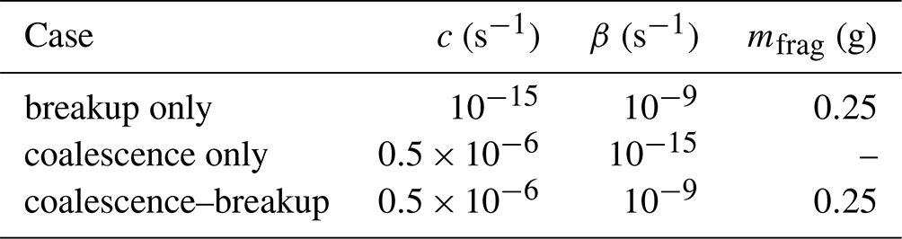
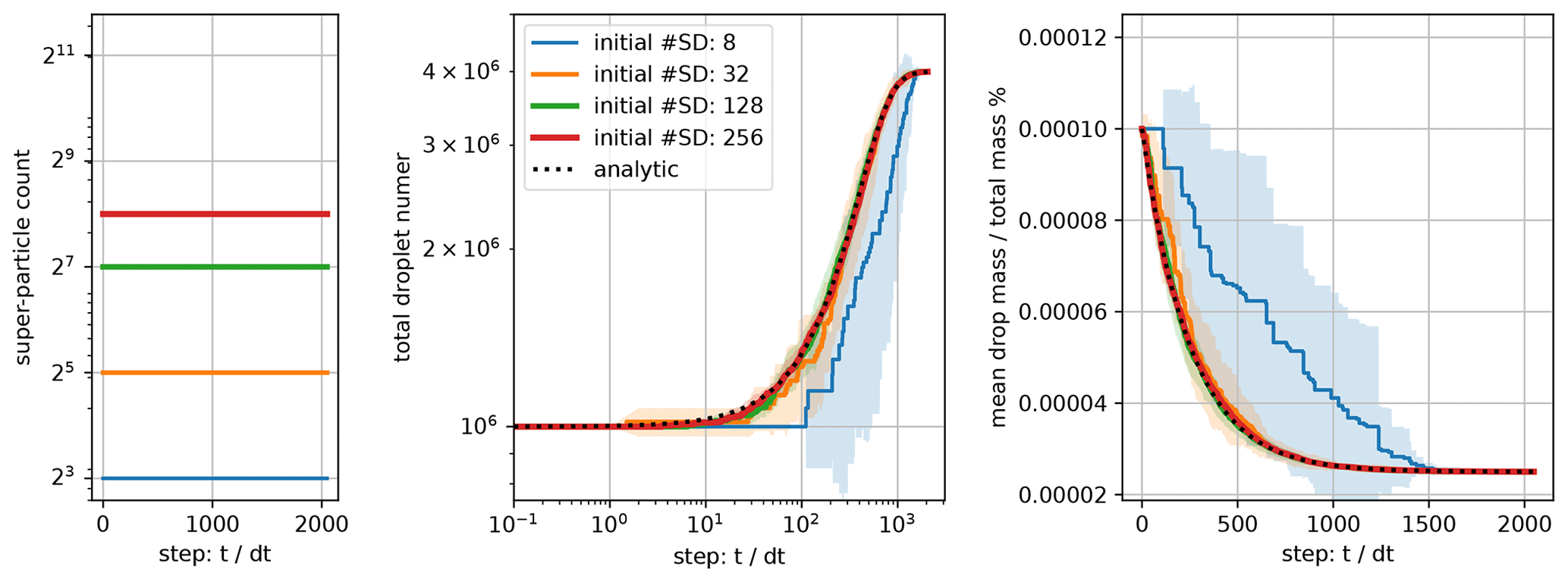
Figure 3 Mean (solid line) and standard deviation (shading) for the time evolution of the breakup-only dynamics, including the analytical solution of Srivastava (1982) and the SDM using 8, 32, 128, or 256 superdroplets.

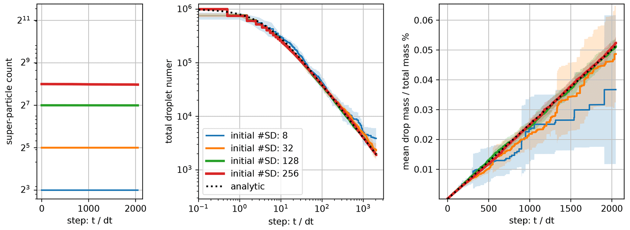
Figure 4 Mean (solid line) and standard deviation (shading) for the time evolution of the coalescence-only dynamics, including the analytical solution of Srivastava (1982) and the SDM using 8, 32, 128, or 256 superdroplets.

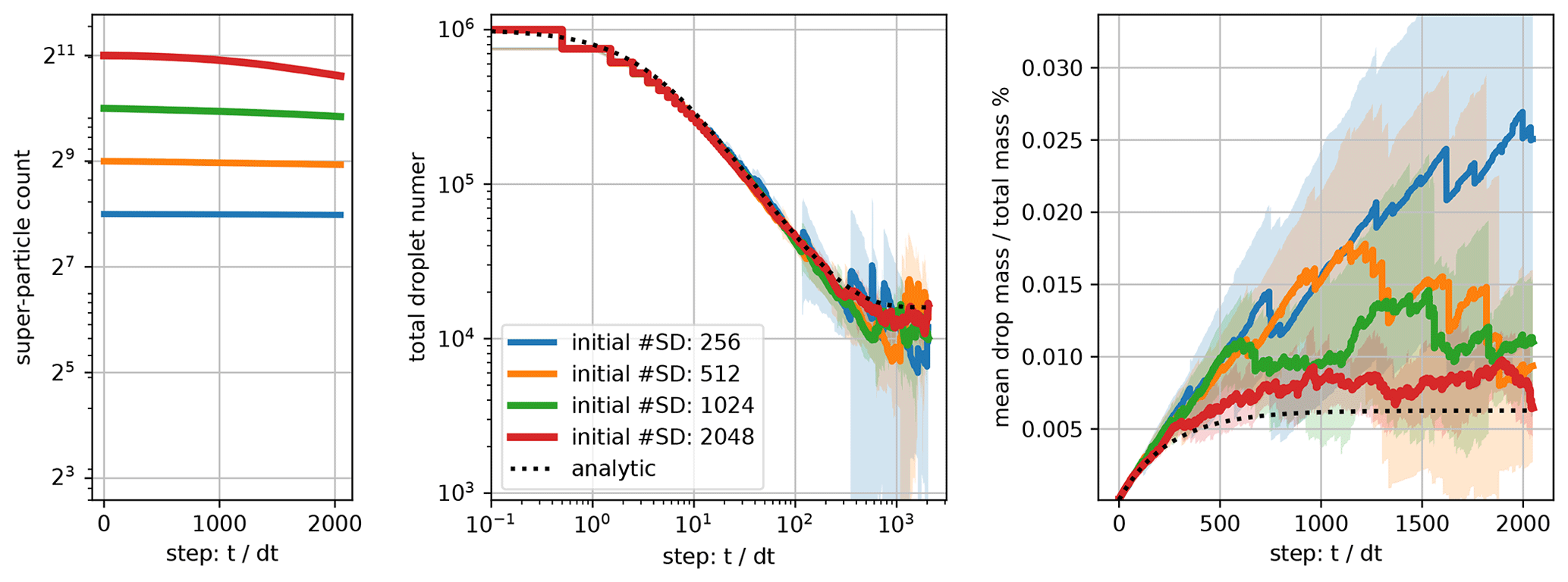
Figure 5 Mean (solid line) and standard deviation (shading) for the time evolution of the coalescence–breakup combined dynamics, including the analytical solution of Srivastava (1982) and the SDM using 256, 512, 1024, or 2048 superdroplets.

Figures 3–5 present the mean and standard deviation of 10 realizations of the SDM simulations versus the analytic solutions. Both the breakup-only (Fig. 3) and breakup-plus-coalescence (Fig. 5) cases feature asymptotic values of droplet number and mass, corresponding to all droplets having the size m_frag (breakup-only case) or a balance between fragmentation and coalescence of droplets (breakup plus coalescence). In all three sets of dynamics, increasing the number of superdroplets robustly reduces the ensemble spread and improves the match with the analytic solution. Much higher resolution (on the order of thousands superparticles) is required to match the analytic solution for the breakup–coalescence equilibrium than for simulations featuring each process separately. This discrepancy is related to the additional stochastic step of selecting the breakup or coalescence dynamic. Extension of this logic implies that even more superparticles would be required to match the exact asymptotic behavior of a system with a distribution of fragment sizes, due to yet an additional stochastic element of sampling.

In Fig. 5, the simulation with the largest number of superdroplets displays the removal of superdroplets from the system. The removal can happen when coalescence leads to zero multiplicity in one of the resultant superdroplets, which then cannot be split into two superdroplets. This is more likely when multiplicities are on average lower (i.e., when more superdroplets are used). In the limit of very few superdroplets, both the breakup-only and the coalescence-only simulations are characterized by underestimation of the process rate, which is consistent with the SDM implementation that neglects collisional dynamics within a superdroplet.

4 Numerical experiments and discussion

To demonstrate the behavior of a particle population under the proposed breakup algorithm, we focus here on sensitivity studies in a zero-dimensional box setting and in a one-dimensional rain-shaft setup. The simulations presented in this section use a geometric collision kernel, where the rate of collisions K_jk between droplets with the properties of superdroplets j and k is given by

$$\begin{array}{}\text{(12)}& {\displaystyle }{K}_{jk}=\mathit{\pi }(R_j+R_k{)}^{\mathrm{2}}|v_j-v_k|,\end{array}$$

where R_j is the radius of particle j and v_j is the terminal velocity/fall speed of particle j, computed using the parameterization of Gunn and Kinzer (1949). As in Shima et al. (2009), collisions within a superdroplet (i.e., collisions between droplets represented by the same superdroplet) are not considered – in line with the use of a geometric collision kernel which precludes collisions between equally sized droplets, as they have the same terminal velocity. (These intra-superdroplet collisions may be important in the case of turbulent collision kernels.)

The coalescence efficiency is specified to be either a constant value (for sensitivity studies) or the empirical coalescence efficiency of Straub et al. (2010) which depends on the Weber number of the colliding droplet pair. (The Weber number is a ratio of kinetic collisional energy and surface tension and relates to the stability of a droplet pair under collision.) We consider three types of fragmentation functions: (1) a constant fragment number N_f, in which the particle size distribution (PSD) is a delta function $P_{\mathrm{f}}\left(m_{\mathrm{f},\mathit{\alpha }}\right)=\mathit{\delta }(m_{\mathrm{f},\mathit{\alpha }}-\frac{m_j+m_k}{N_{\mathrm{f}}})$; (2) an exponential distribution $P_{\mathrm{f}}\left(m_{\mathrm{f},\mathit{\alpha }}\right)\sim \exp (-m_{\mathrm{f}}/\mathit{\mu })$, where the scale μ is specified; and (3) the empirically derived fragmentation function of Straub et al. (2010), which uses four modes of fragmentation represented by lognormal or normal subdistributions.

4.1 Particle size distribution

The zero-dimensional box simulations include collisional-coalescence and collisional-breakup dynamics only. The droplet size distribution is initialized to an exponential distribution in mass x, given by $N\left(x\right)=x_{\mathrm{0}}\exp (-x/x_{\mathrm{0}})$ with the characteristic size $x_{\mathrm{0}}=(\mathrm{4}\mathit{\pi }/\mathrm{3})R_{\mathrm{0}}^{\mathrm{3}}$ set using R₀=30.531 µm as in Shima et al. (2009). The simulations employ 2¹³=8192 superdroplets to represent a number density of 100 cm⁻³ in a box of volume 1 m³ with a fixed time step of 1 s. This choice of superdroplet quantity is sufficient to produce consistent results in the PSD across realizations using a different random seed and was shown by Shima et al. (2009) to closely match the exact PSD in a similar box model simulation of collisional coalescence.

Particle size distributions are displayed as the number distribution or as the marginal mass distribution $g\left(R\right)=\frac{\mathrm{d}m}{\mathrm{d}\ln \left(R\right)}=\mathrm{3}{x}^{\mathrm{2}}n\left(x\right)$, where n(x) is the particle size distribution. This mass distribution is computed by binning the resulting superdroplets into 128 logarithmically spaced size bins between particle radius 1 µm and radius 10 mm. We separate the simulations into those which use a deterministic fragmentation function, in which breakups result in a constant number of fragments in any given collision; a stochastic fragmentation function with fragment sizes sampled from a specific distribution; and a size-dependent fragmentation function, where the fragment sizes are sampled from a distribution whose parameters depend on the colliding particles. We further include experiments exploring the use of a fixed coalescence efficiency versus a particle-attribute-derived coalescence efficiency. This separation elucidates which aspects of the particle population behavior are attributable to stochastic sampling of the fragmentation function or related to particle-property-dependent parameters such as Weber number.

4.1.1 Sensitivity studies: deterministic and size-independent fragmentation

First we investigate the sensitivity of the PSD evolution to the coalescence efficiency, using four values of a constant-valued efficiency E_c between 0.7 and 1.0 (E_c=1.0 corresponds to coalescence only) and a particle-size-dependent E_c parameterization (Straub et al., 2010). All simulations use a deterministic fragmentation function in which all single-step collisional breakups result in N_f=8 fragments:

$$\begin{array}{}\text{(13)}& {\displaystyle }{P}_{\mathrm{f},\mathit{\alpha }}\left(m_{\mathrm{f}}\right)=\mathit{\delta }\left(m_{\mathrm{f}}-{\displaystyle \frac{m_j+m_k}{N_{\mathrm{f}}}}\right).\end{array}$$

Figure 6 displays two snapshots of the PSD under this set of dynamics, demonstrating the additional Monte Carlo step of selecting whether coalescence or breakup occurs, independent of sampling a fragment size. As expected, the initial PSD broadens and shifts toward larger droplets at 100 s, with the largest values of fixed E_c leading to the largest increase in average particle mass. However, after 200 s, the PSD for the E_c=0.8 case remains approximately steady with a mean size that is smaller than the initial distribution mean, demonstrating that coalescence and breakup are approximately balanced in this case.

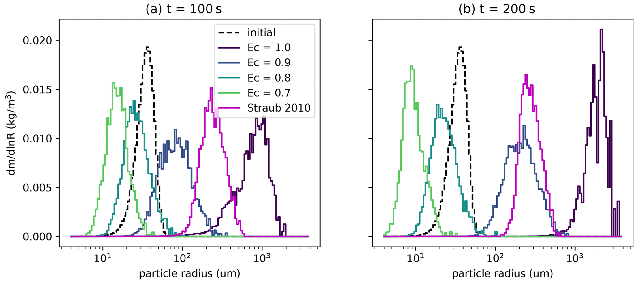
Figure 6 Particle size distribution with varying coalescence efficiencies under a geometric collision kernel after 100 s (a) and 200 s (b). The breakup fragmentation function is deterministic, with the fragment size determined as one-eight of the sum of the colliding droplet sizes. The dashed black line represents the initial PSD, and solid lines represent various fixed values of the coalescence efficiency. The pink line corresponds to a size-dependent coalescence efficiency from Straub et al. (2010).

By contrast, the PSD for the Straub 2010 parameterization of E_c is initially between the E_c=0.9 and E_c=1.0 simulations at 100 s but narrows without shifting toward much larger droplets after further time has elapsed, leading to a dominant mode that is more similar to the E_c=0.9 case. This empirical parameterization also shows evidence of approaching a steady-state distribution, in which coalescence and breakup rates are matched on average, driving the PSD to a stationary state. The Straub 2010 parameterization decreases exponentially with the colliding particle Weber number, which is correlated with the size and relative terminal velocity of the colliding particles. Two colliding particles of comparable size have a low relative terminal velocity; therefore, as the PSD shifts toward larger coalesced droplets, there is a competing effect between a larger particle size increasing the Weber number and decreased relative terminal velocity reducing it. This competition produces the stationary behavior and narrowing of the PSD observed in this case.

Figure 7 Sensitivity to fragmentation function of PSDs following collisions with a geometric kernel and fixed coalescence efficiency of E_c=0.95 in a deterministic and stochastic fragmentation function case. (a) The fragment size is fixed by a divisor of the sum of colliding particle volumes; (b) fragment size is sampled from an exponential distribution with varying means μ determined as a multiple of the initial distribution mean. The initial distribution is shown as a dashed black line in each figure.

Next we consider the PSD evolution when the coalescence efficiency is held fixed at a constant value and the fragmentation function is varied. In Fig. 7a, we consider a deterministic fragmentation function where the number of fragments from a single breakup event is fixed (as in Fig. 6), as well as an exponential fragment size distribution with scale μ specified as a multiple of the initial mean particle mass x₀. When the number of fragments is fixed, results using the largest number of fragments display the smallest mean particle size and broadest spectra. The first behavior is expected, as a larger value of N_f results in smaller typical fragment sizes. The broadening of the spectrum can be attributed to a wider range of collision rates between very small droplets (which result from fragmentation) and is generally an expected outcome of including collisional breakup.

When the fragment size is sampled from an exponential distribution (Fig. 7b), the resulting spectra are bimodal, with a large-droplet mode that is larger for larger choices of the mean fragment size μ and a narrow small-droplet mode that likewise depends on μ. The appearance of a second mode occurs when the fragment size is sampled from the left tail of the fragment size distribution, whereas the large mode corresponds to a droplets undergoing coalescence only, as in the N_f=1 case. This behavior indicates that through stochastic sampling of the dynamic and fragment size together, the droplet population splits into one mode which fragments into smaller droplets and a second mode which primarily undergoes coalescence and grows in size. Because larger droplets collide at much quicker rates than small droplets, the fragmented mode is less likely to collide and re-coalesce to form medium-sized droplets, while the coalesced mode retains some probability of colliding and either growing (coalescing) or breaking up into smaller droplets. Thus, we observe that the small-droplet-mode grows in this instance, with particles effectively becoming “stuck” in this dynamical regime due to the separation of scales in collision rates.

4.1.2 Steady state under stochastic size-dependent fragmentation

Finally, we consider an empirically derived coalescence efficiency and corresponding fragmentation function whose parameters depend on the colliding droplet properties (Straub et al., 2010). In Fig. 8, we consider the evolution of the PSD under the Straub 2010 efficiency and fragmentation dynamics, beginning from the same initial distribution as previous experiments. At first, the PSD broadens and shifts towards larger droplet sizes, as in Fig. 6, but the PSD after 7200 s shows little difference from the PSD at 1800 s. These results indicate the stationarity of the particle size distribution after sufficient time has elapsed: coalescence and breakup are balanced, as in the previous example. Contrasted with Fig. 6, which used a deterministic size-independent fragmentation function, the stationary PSD resulting from the Straub et al. (2010) parameterization of fragmentation is less symmetric and contains multiple small peaks. This difference reflects the sampling from a multimodal distribution of fragment sizes, contrasting with the symmetric PSDs found from using a fixed number of fragments.

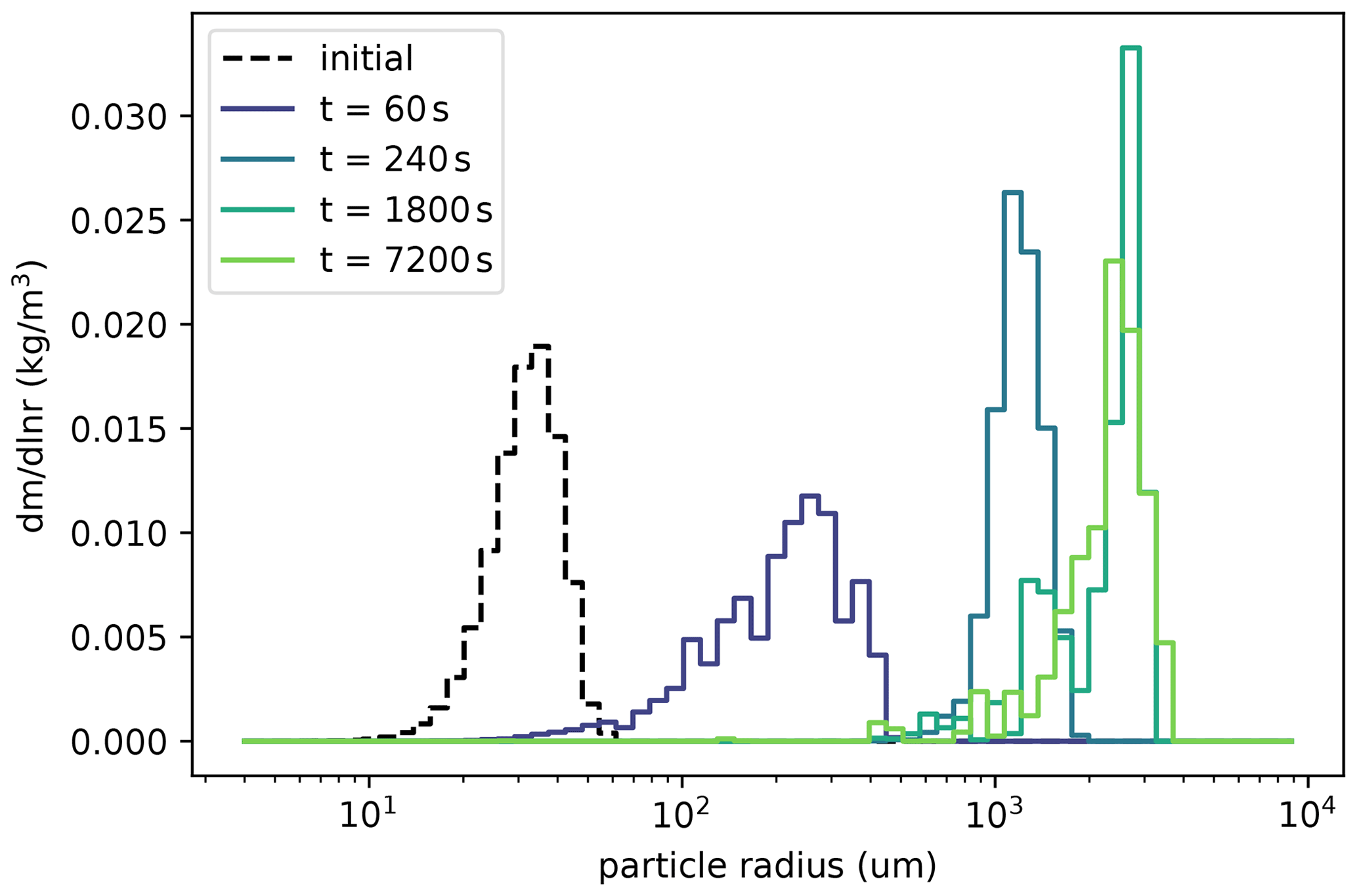
Figure 8 Initial PSD (dashed black) and PSDs following collisions with a geometric kernel, the Straub 2010 collection efficiency, and the Straub 2010 fragmentation function (Straub et al., 2010) after several elapsed times (colors).

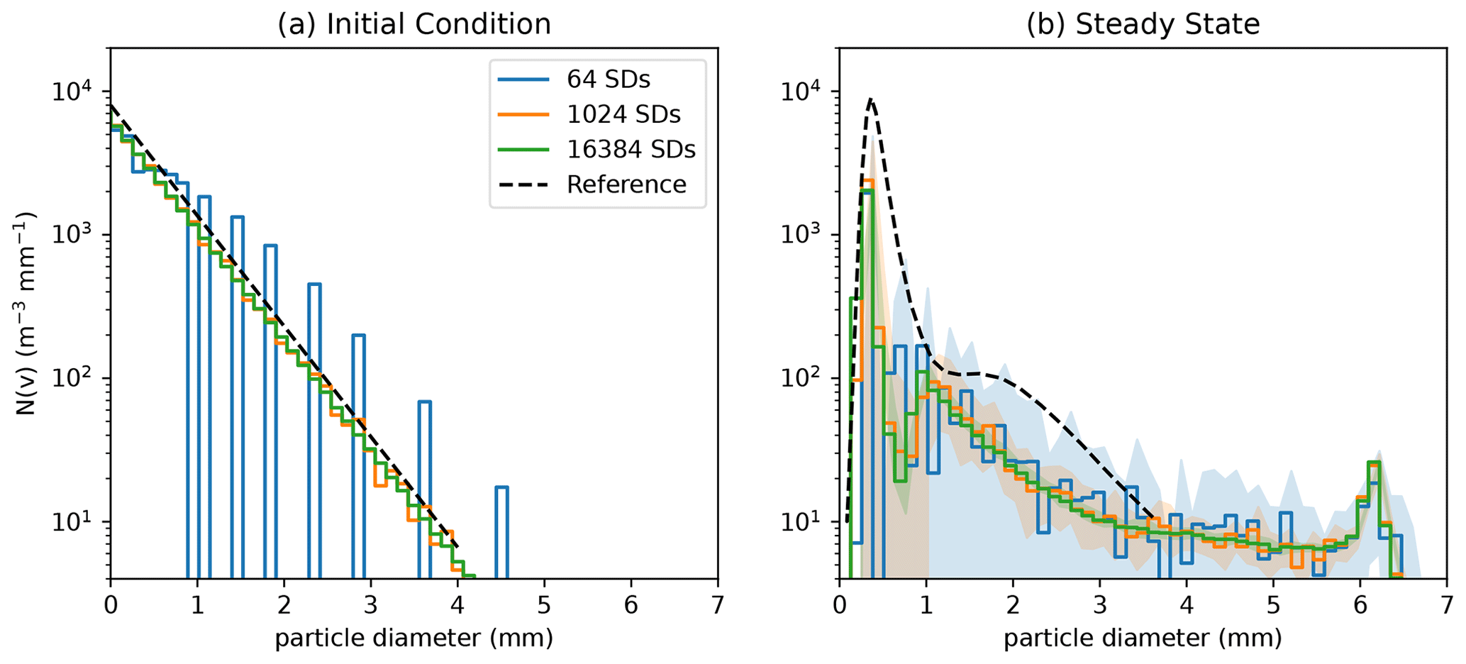
Figure 9 Initial PSD (a) and steady-state PSD (b) under collisions with the Straub 2010 parameterizations, including reproduction of the findings in Fig. 10 from Straub et al. (2010) (dashed black line), and simulations including the proposed breakup algorithm with different numbers of superdroplets. Steady-state results are displayed as the mean plus or minus 1 standard deviation (shading) of 10 simulation instances.

This empirical parameterization provides an additional opportunity for validation of the breakup algorithm on top of the analytical results presented in Sect. 3. Figure 9 compares results of this SDM implementation against Fig. 10 of Straub et al. (2010) (note that we now plot number concentration rather than mass concentration with a logarithmic y scale and linear x scale, as in Straub et al., 2010 and McFarquhar, 2004). Particles are initialized as a Marshall–Palmer distribution (exponential in droplet diameter) with rain rate 54 mm h⁻¹; superdroplet sizes are sampled logarithmically over this diameter range rather than using constant multiplicity. With only 64 superdroplets, the SDM struggles to adequately sample the low concentration but important rain droplets with diameters exceeding 1 mm, while using over 1000 superdroplets is more than sufficient. The simulation is run using a 1 s time step for 7200 s to approximate a steady state in Fig. 9b. The SDM appears to converge using between 1000 to 16 000 superdroplets, with more superdroplets being necessary to reduce spread of the results for small particle diameters. The SDM approach captures the size and amplitude of the first mode of the steady-state distribution reasonably well, but shows some discrepancies at intermediate particle sizes, predicting a secondary mode at 1.2 mm diameter rather than the less pronounced shoulder at 2 mm. Inspecting the resulting distributions at large particle sizes reveals a larger quantity of 6–7 mm diameter particles in the SDM simulations, which are not seen in the work of Straub et al. (2010). This behavior indicates that some large superdroplets coalesce rather than breaking up, which may be reflective of the multiplicity limiter in the model which performs coalescence rather than breakups which would result in a very large increase in multiplicity (i.e., sampling a small fragment size during collision involving one or more large droplets). The coalescence efficiency tends toward zero for any droplet larger than 6 mm in diameter, which explains why the large-droplet mass is concentrated at this size. In a realistic setting, however, most rain-range droplets would be expected to sediment before attaining this large 6 mm size through coalescence. Indeed, we note that later results presented in Fig. 11 do not show significant mass concentration at droplet sizes larger than 1 mm radius, indicating that this error in the steady state does not present in the transient rain-shaft simulation.

4.2 Cloud and precipitation properties

Next we consider the impact of collisional breakup in a one-dimensional warm-rain setting that includes condensation/evaporation (including aerosol activation/deactivation), collisions, and transport of particles within the column through advection and sedimentation/precipitation. These 1D simulations are based on the kinematic framework of Shipway and Hill (2012), using a fixed profile of dry-air potential temperature and dry-air density ρ_d(z), and a resolved budget of water vapor (advection and coupling with vapor uptake and release by particles). The vapor advection is solved using the MPDATA algorithm on a columnar grid with vertical spacing of 100 m (employing the PyMPDATA implementation, Bartman et al., 2022a). An aerosol population with hygroscopicity κ=0.9 is initialized throughout the vertical domain with 2⁸=256 superdroplets per grid box. This choice of 256 superdroplets per grid box reflects the higher computational demands of the one-dimensional simulation compared to the box model and still produces statistically convergent results in the macroscopic quantities investigated. For the first 600 s of spin-up, condensation–evaporation (including aerosol activation using kappa-Köhler theory; implementation of these processes follows that of Arabas et al., 2015) and particle advection with the specific updraft are the only active dynamics, with a time-varying updraft momentum flux of ρ_dw(t)=6  kg m⁻³ m s${}^{-\mathrm{1}}\sin (\mathit{\pi }t/\mathrm{600}\mathrm{s})$. After this spin-up time, the updraft velocity is set to 0, and the processes of particle displacement due to sedimentation and collision–coalescence–breakup begin. The time step is fixed at 5 s throughout the simulation.

The test cases demonstrated here include a no-breakup case, a property-independent breakup case where the coalescence efficiency is fixed and fragment sizes are sampled from a fixed distribution, and the particle-property-dependent empirical coalescence efficiency and fragmentation parameterizations from Straub et al. (2010). All simulations use a geometric collision rate (Eq. 12) and the Gunn and Kinzer (1949) terminal velocity parameterization. In the no-breakup case, all collisions result in coalescence. In the property-independent breakup case, we fix E_c=0.95 for all superdroplet collisions based on the correspondence in Fig. 6 to the empirical coalescence efficiency. This case samples fragment sizes from a Gaussian distribution in particle volume with mean radius 30 µm and standard deviation 15 µm. In contrast to the property-independent case, in which the fragmentation parameters are hand-selected, the property-dependent setting is based on empirical evidence and is expected to be more reflective of the variability of real clouds. In both the property-independent and property-dependent cases, the breakup efficiency is set to E_b=1 such that all collisions result in either coalescence or breakup. To contrast the behavior of the three cases, we consider the hydrometeor population at various altitudes throughout the simulation, as well as collision process rates and aerosol processing rates.

4.2.1 Hydrometeor and cloud quantities

The mixing ratio of cloud droplets (activated droplets of no more than 50 µm radius), the mixing ratio of rain droplets (radius greater than 50 µm), and the number concentration of unactivated aerosols are displayed for the three test cases in Fig. 10. The no-breakup simulation forms a cloud due to activation of aerosols between 600 and 3800 m altitude until the updraft is terminated after 600 s. Larger rain-range droplets form from collisional coalescence and begin to sediment out of the system in clusters, visible as distinct streaks in the (t,z) plane, with surface precipitation beginning around 1100 s into the simulation, depleting the cloud droplet population. The vertically averaged particle size spectra in Fig. 11 demonstrate these qualitative changes as well. At 600 s, the majority of particles are micron-sized aerosols with cloud droplets beginning to form. At later times of 900 and 1200 s, the particles rapidly grow to tens or hundreds of microns in size, and at 1800 s, the mass distribution in the no-breakup case shows significant depletion due to precipitation of large particles.

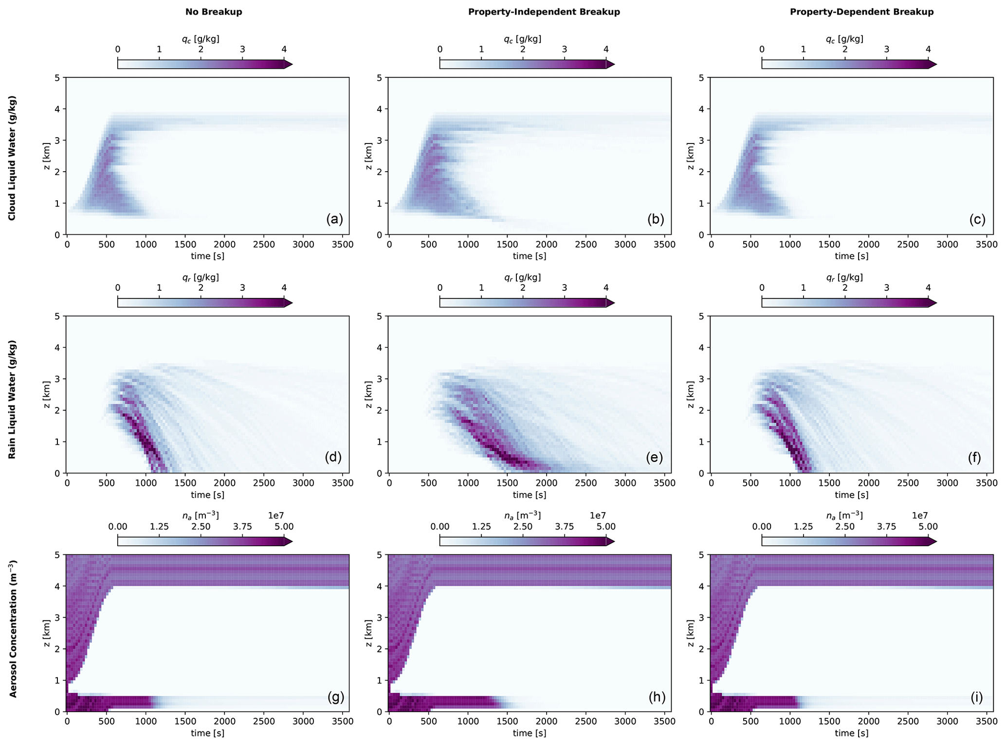
Figure 10 Hydrometeor concentrations without breakup (a, d, g), with breakup using a property-independent coalescence efficiency (b, e, h), and with breakup following the property-dependent Straub et al. (2010) parameterizations (c, f, i). Included are cloud water mixing ratio (a, b, c), rain water mixing ratio (d, e, f), and aerosol number concentration (g, h, i).

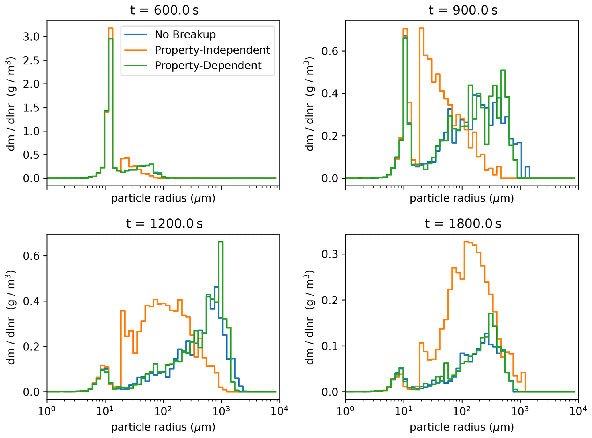
Figure 11 Vertically averaged particle size spectra (as a marginal mass distribution) at four times selected from the 1D rain-shaft simulations for each set of dynamics (colors).

When property-independent breakup is included, a higher concentration of cloud-sized droplets persists at cloud base, and the surface precipitation is delayed and spread out relative to the case with no breakup. This behavior indicates that rain droplets favorably break up within the cloud and especially near cloud base, fragmenting into smaller cloud droplets (the mean of the fragment size distribution is 30 µm radius, only slightly lower than the rain size range) with a lower sedimentation rate. We observe this behavior in Fig. 11 as well: the property-independent case shows much smaller average particle sizes at 900 and 1200 s, as well as more mass remaining in the system at 1800 s due to the delayed precipitation. Furthermore, the aerosol population below cloud base is not depleted as quickly in this property-independent case, indicating a reduction in aerosol scavenging and washout that is consistent with the lower precipitation rates. These phenomena are consistent with documented impacts of collisional breakup such as reduced surface precipitation (Seifert et al., 2005) and show that the proposed algorithm can meaningfully represent the breakup process.

The empirical property-dependent breakup case using the Straub et al. (2010) parameterizations displays hydrometeor populations that are more similar to the no-breakup case, indicating that the choice of E_c=0.95 in the property-independent case likely overestimates the rate of collisional breakup when condensation and evaporation are present (contrasted with Fig. 6). As in the no-breakup case, the property-dependent empirical case displays distinct streaks of precipitation, with surface precipitation initiated around 1100 s. While the hydrometeor populations show only slight differences between no-breakup and property-dependent breakup in Fig. 10, the size spectra at 900 s in Fig. 11 shows a somewhat narrower size distribution for the property-dependent case as particles approach the rain size range, suggesting the role of collisional breakup.

The relatively short updraft time and simple one-dimensional representation of this setup produce a short-lived cloud that is precipitating for only a few minutes. The likelihood of breakup in the Straub parameterization is strongly correlated with the size of the colliding droplets, with E_c approaching 1 for colliding droplets smaller than 1 mm diameter; therefore, we expect to see a stronger impact of including SDM breakup in a strongly precipitating convective case. Due to the complexity and feedbacks inherent to representing a superdroplet-coupled flow field as well as mixed-phase processes, such experiment is beyond the scope of the present work focused on the algorithm formulation. In deeper mixed-phase clouds, however, secondary ice production via ice–ice and ice–supercooled-liquid collisions are two analogous processes of collisional breakup that may be important (Hallett and Mossop, 1974; Harris-Hobbs and Cooper, 1987; James et al., 2021; Zhao and Liu, 2022). Multiphase superdroplet representation of these mechanisms will face a similar challenge of representing many different fragment sizes; thus, the SDM breakup representation presented in this work could be extended to collisional ice processes in future research on secondary ice production and mixed-phase clouds.

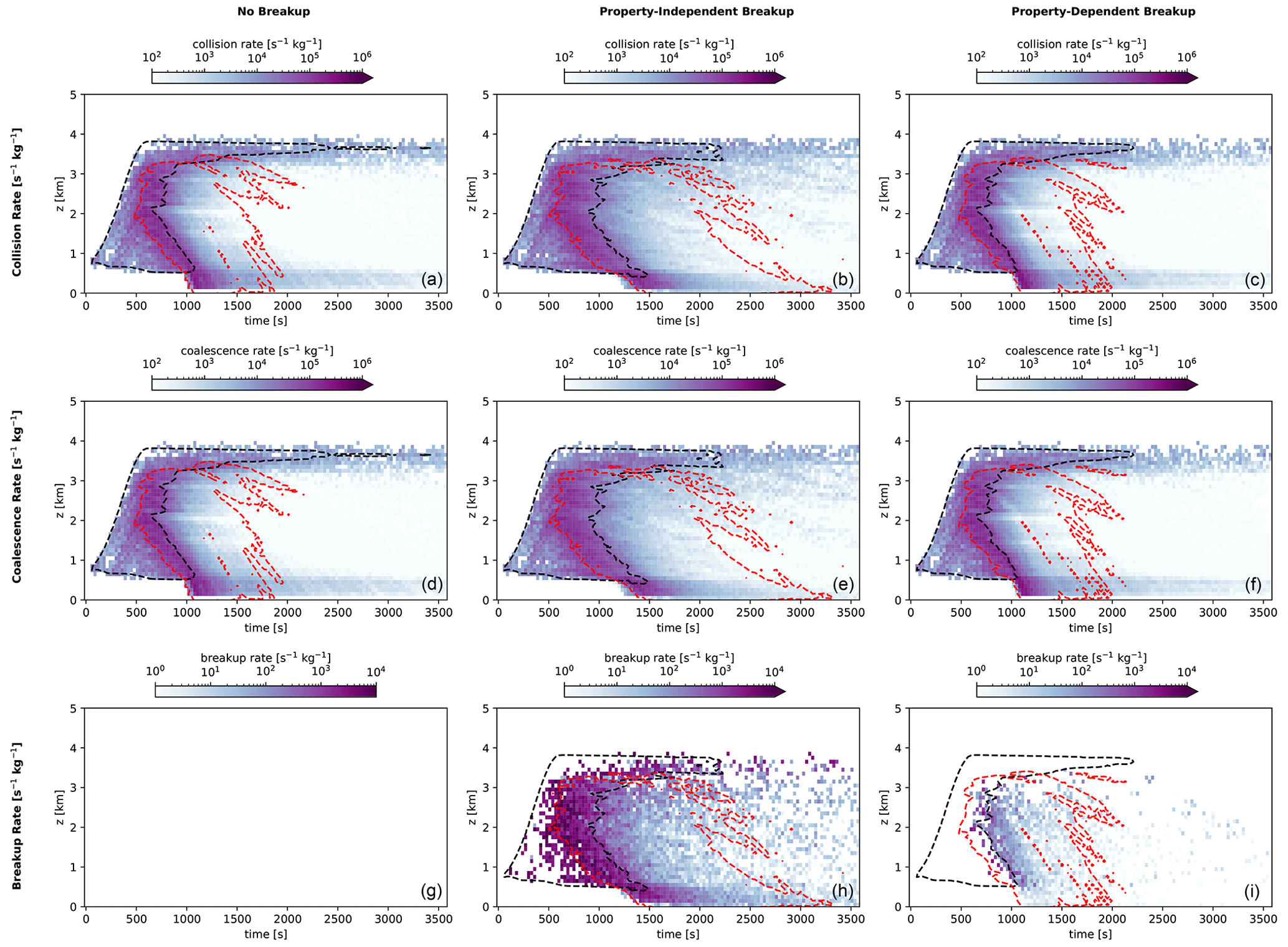
Figure 12 Collisional dynamic rates for the one-dimensional case with (a, d, g) no breakup, (b, e, h) breakup with a fixed coalescence efficiency, and (c, f, i) breakup with the Straub 2010 parameterizations. The dynamics shown include (top to bottom) collision rate, coalescence rate, and breakup rate. Dashed contour lines represent the level of q_c=0.4 g kg⁻¹ (black) and q_r=0.4 g kg⁻¹ (red), representing a cloudy and rainy region of the time–space domain, respectively.

4.2.2 Process rates

Figure 12 displays the local rates of superdroplet collision (scaled by multiplicity), as well as distinguishing between rates of coalescence and rates of breakup. We see an expected correlation between the time and location of collisions in all three cases with the location of hydrometeors (outlined in black for cloud and red for rain) – as expected, a higher concentration of hydrometeors, particularly large rain-range hydrometeors, corresponds to higher rates of all collisional dynamics. The rate of collisions increases throughout the simulation time, particularly near cloud base where the largest droplets are sedimenting and colliding at higher rates. The property-independent case is consistent with the other cases in displaying higher collision rates at cloud base, even though the droplets in this region are slightly smaller and fall in the cloud category.

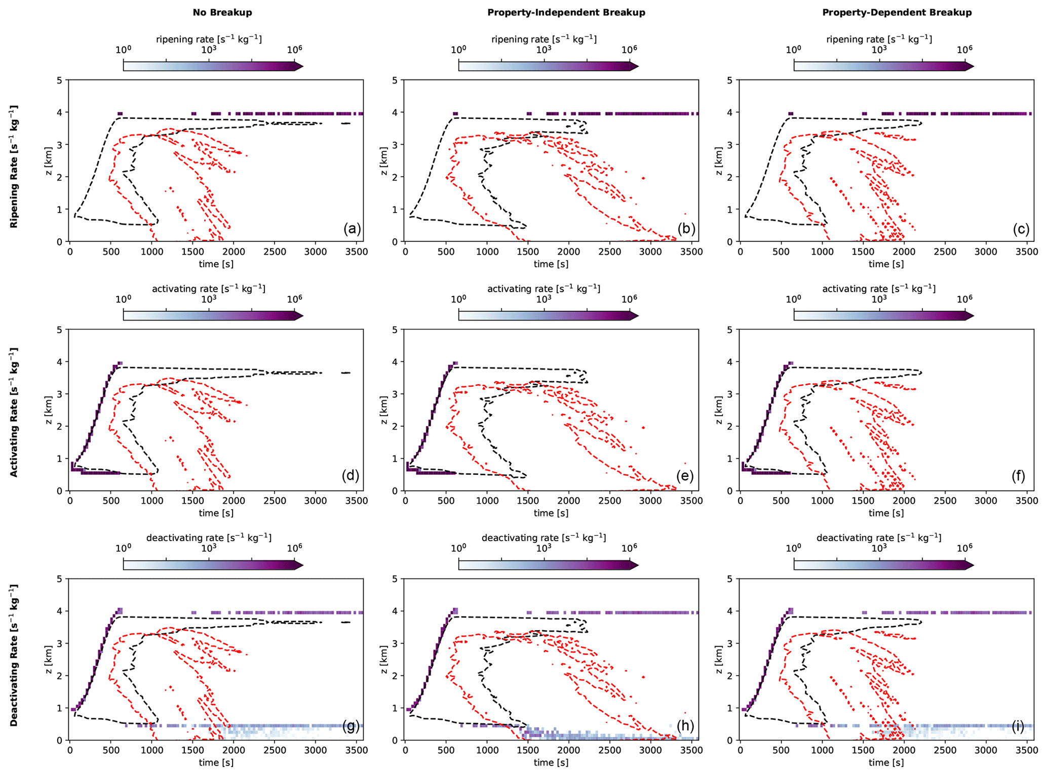
Figure 13 Aerosol processing rates for (left to right) no breakup, property-independent breakup, and Straub et al. (2010) parameterizations. Included are (top to bottom) ripening rate, activating rate, and deactivating rate. Dashed contour lines represent the level of q_c=0.4 g kg⁻¹ (black) and q_r=0.4 g kg⁻¹ (red), representing a cloudy and rainy region of the time–space domain, respectively.

All three cases display similar rates of collision and coalescence, with the highest of these rates occurring in the cloud among rain droplets and below cloud base among precipitating rain droplets. In the no-breakup case, every feasible collision results in a coalescence, and the breakup rate is zero. When property-independent breakup is included, the time–space distribution of the breakup rate is nearly identical to that of the collision rate. This trend is consistent with the use of a uniform coalescence efficiency E_c=0.95, which is agnostic to the size of the colliding particles. In contrast, the empirical property-dependent case sees collisional breakup primarily where larger rain droplets are present, consistent with the Straub et al. (2010) parameterization based on Weber number. Breakup events drop off quickly after the initial depletion of the cloud-sized droplets, as the coalescence efficiency for two large particles is much smaller than that of a small particle colliding with a large particle. As seen in Fig. 11, breakup plays less of a role in determining the hydrometeor populations after 1200 s of simulation time. Thus, the impacts of collisional breakup are limited in time and space to where large concentrations of hydrometeors of both cloud and rain size are colliding. These results demonstrate that the SDM breakup algorithm can produce expected process behavior both in a property-independent setting, where the collision dynamics result in strong breakup, and in an empirically parameterized setting.

As noted in the discussion of Fig. 10, the property-independent breakup case experiences a persistent population of aerosols below cloud base until 1500 s, while the no-breakup and property-dependent cases demonstrate washout upon the earlier onset of precipitation. Collisional breakup resulting in very small droplet fragments could potentially introduce cloud droplets so small that they deactivate in their environment. In Fig. 13, we investigate whether collisional breakup can induce significant changes to aerosol processing rates, considering aerosol activation, deactivation, and ripening.

The property-independent and no-breakup cases have nearly identical behavior in aerosol processing, consistent with the correspondence between their hydrometeor concentrations and collision process rates. In all three cases, a few superdroplets at cloud top encounter humidity close to their critical supersaturation, which results in the “ripening” processes of fluctuation between an activated and deactivated state due to competition when the supersaturation is insufficient to activate all aerosols (e.g., Arenberg, 1939; Wood et al., 2002). (We define ripening rate as the number of activated droplets growing through condensation per unit of time within a grid cell in which deactivation simultaneously occurs on other particles). Aerosols activate primarily at the start of the simulation when an updraft is present, defining the altitude boundaries of the cloud. No additional activation is seen in either instance including collisional breakup. Deactivation occurs among a few aerosols which activate and then rise in altitude beyond cloud top initially and more strongly below cloud base as droplets sediment out of the cloud and evaporate. The property-independent case experiences much stronger deactivation at cloud base, which corresponds to the higher rate of fragmentation of droplets at this altitude. The no-breakup and property-dependent breakup cases display continued deactivation of aerosols at the cloud base height throughout the simulation, while the property-independent case shows only near-surface deactivation, suggesting aerosol scavenging by rain droplets throughout the more sustained precipitation process. These results indicate that collisional breakup could be a relevant process for future studies of aerosol-cloud effects, particularly in deeper-convective cases where collision rates are likely to be higher.

5 Conclusions

This work presents a superdroplet algorithm for collisional breakup that is scalable in avoiding creation of new superdroplets and physical in its ability to produce results in a box and one-dimensional setting that are consistent with the expected reduction and delay in rain formation. Furthermore, the algorithm produces hydrometeor populations and process rates that differ between a property-independent approach (with a fixed coalescence efficiency and fixed fragment size distribution) and a property-dependent approach using empirical parameterizations. These differences indicate the importance of random, stochastic events in warm-rain microphysics, a trait which has also been documented in other microphysical phenomena such as giant cloud condensation nuclei (CCN; Feingold et al., 1999; Yin et al., 2000). Without a scalable representation, the superdroplet method has heretofore been unable to capture these additional stochastic impacts of breakup, and it has not been applied to compare empirical parameterizations of coalescence and breakup, which contribute uncertainties to operational process, weather, and climate models.

This work provides the basis for a more complete representation of microphysical processes in particle-based simulations. For instance, a superdroplet representation that considers ice-phase hydrometeors and properties could probe processes of secondary ice production such as fragmentation and freezing of supercooled water droplets upon collision with ice (James et al., 2021), rime splintering (Hallett and Mossop, 1974), or ice–ice collisions (Harris-Hobbs and Cooper, 1987; Phillips et al., 2017). These and other mixed-phase processes are poorly understood due to challenges in obtaining direct observational or laboratory measurements; thus, a high-fidelity particle-based representation such as the superdroplet method provides an ideal means for studying these phenomena. While the collisional breakup representation presented here does not address underlying uncertainties in parameterization of processes such as collision rates and phase change, it provides a path forward for more rigorous and complete studies of cloud microphysics.

Appendix A: Limiters

In implementing collisional breakup for superdroplets, we suggest imposing a few limiters to enforce physical constraints and maintain stability of the code. If the user-selected time step for the SDM implementation is too large, collisional breakup may quickly become a runaway process with superdroplet multiplicities increasingly rapidly and unphysically, leading to numerical overflow. As an example, suppose a droplet of multiplicity 10² should undergo six collisional breakups (γ_α=6) into five fragments each time ($N_{\mathrm{f},\mathit{\alpha }}=\mathrm{5}$): then γ_jk=3906 and its new multiplicity is 15 525=𝒪(10⁴). Successive collisional breakups between droplets whose multiplicities have grown so rapidly would then lead to exponentially booming multiplicities and could quickly exceed the maximum representable quantity for the computing machine (overflow). One solution is to set a maximum allowable multiplicity for any superdroplet and to reject any collisional breakups that would produce a superdroplet exceeding this multiplicity.

In addition, the process of collisional breakup is physically constrained such that the resulting superdroplet (the fragment) volume should not exceed the volume of the coalesced transition state, nor should it drop below a realistic size for a liquid water droplet (molecule scale, for instance). These physical constraints can be imposed by setting a minimum and maximum allowable fragment size resulting from breakup.

The first of these constraints can then be imposed during computation of γ_jk within the while loop in Eq. (7):

$$\begin{array}{}\text{(A1)}& {\displaystyle }{\mathit{\xi }}_k^{\text{new}}{\displaystyle }\le {\mathit{\xi }}_{max},\end{array}$$

where ξ_max is a maximum multiplicity set to prevent overflow. The second two constraints are imposed during the sampling of a fragment size:

$$\begin{array}{}\text{(A2)}& {\displaystyle }{m}_{min}\le m_{\mathrm{f},\mathit{\alpha }}\le m_j+m_k,\end{array}$$

where m_min is a minimum physically allowed fragment size.

Appendix B: Sampling from empirical fragment size distributions

Sampling a fragment size m_f,α requires selecting at random one m_f,α according to its weight in the overall fragment size distribution. For fragmentation functions which are composed of several distinct modes, modes must be additionally mass-weighted according to the mode's associated fragment sizes in order to attain the correct expectation value of fragment mass in the resulting sample. A common way of sampling from simple distributions, such as a normal or lognormal, is to invert the CDF (cumulative distribution function). We will demonstrate how to extend this procedure to an empirical fragmentation function comprised of several modes, which lacks a closed-form CDF. For instance, the commonly used fragmentation function of Low and List (1982) partitions the fragmentation physics into three categories, corresponding to filament, sheet, and disk breakup. Each category is then comprised of two to three modes, corresponding to smaller satellite fragments and larger remnants of the parent droplets. Similarly, Straub et al. (2010) distinguish four categories of fragments, with the fragment size distribution within each category following a lognormal or normal distribution. (Here, we follow the notation of Straub et al., 2010.)

Suppose the unnormalized fragmentation function P_f(D) in droplet diameter D is described as a sum of k modes:

$$\begin{array}{}\text{(B1)}& {\displaystyle }{P}_{\mathrm{f}}\left(D\right)=\sum _{r=\mathrm{1}}^k{N}_r{p}_r\left(D\right),\end{array}$$

where N_r is the expected number of fragments from mode r, and p_r(D) is the normalized fragment size distribution for mode r. We begin by re-weighting the size distribution by the mass contained within each mode, M_r,

$$\begin{array}{}\text{(B2)}& {\displaystyle }{M}_r=\underset{\mathrm{0}}{\overset{\mathrm{\infty }}{\int }}{\displaystyle \frac{\mathit{\pi }}{\mathrm{6}}}{D}^{\mathrm{3}}{p}_r\left(D\right)\mathrm{d}D,\end{array}$$

and then normalizing the distribution such that its integral is unity,

$$\begin{array}{}\text{(B3)}& {\displaystyle }{P}_{\mathrm{f},n}\left(D\right)={\displaystyle \frac{{\sum }_{r=\mathrm{1}}^k{N}_r{M}_r{p}_r\left(D\right)}{{\sum }_{r=\mathrm{1}}^k{N}_r{M}_r}}.\end{array}$$

These initial transformations yield a normalized fragment size distribution which contains all modes of the fragmentation function weighted according to mass. P_f,n(D) corresponds to the probability (as a fraction) of retrieving a sample of mass D given the colliding droplet parameters.

Next, to sample a single fragment size D_f, we first use the random number ${\mathit{\varphi }}_{\mathit{\alpha }}^{\prime \prime }$ to determine which mode of the overall distribution is sampled. This equates to finding s such that

$$\begin{array}{}\text{(B4)}& {\displaystyle \frac{{\sum }_{r=\mathrm{1}}^{s-\mathrm{1}}{N}_r{M}_r}{{\sum }_{r=\mathrm{1}}^k{N}_r{M}_r}}\le {\mathit{\varphi }}_{\mathit{\alpha }}^{\prime \prime }<{\displaystyle \frac{{\sum }_{r=\mathrm{1}}^s{N}_r{M}_r}{{\sum }_{r=\mathrm{1}}^k{N}_r{M}_r}}.\end{array}$$

The resulting fragment will represent only a single mode of the overall fragment size distribution. However, selecting the mode according to its mass-weighted probability conserves the expected mass distribution of the fragmentation function. The average of several such steps is more likely to sample from each mode; therefore, it is crucial that a small enough time step is chosen to allow convergence of this stochastic selection across collisions.

Next, the fragment size is chosen by sampling at random from the CDF of the mode p_s(D), which is assumed to be approximable by a closed-form equation (as in the case of a Gaussian or lognormal distribution). This second step of sampling can be accomplished by selecting a new random number, reusing the random number from a different colliding droplet pair, or simply rescaling ${\mathit{\varphi }}_{\mathit{\alpha }}^{\prime \prime }$ as

$$\begin{array}{}\text{(B5)}& {\displaystyle }\stackrel{\mathrm{̃}}{{\mathit{\varphi }}_{\mathit{\alpha }}^{\prime \prime }}={\displaystyle \frac{{\mathit{\varphi }}_{\mathit{\alpha }}^{\prime \prime }-{\sum }_{r=\mathrm{1}}^{\mathrm{s}-\mathrm{1}}{N}_r{M}_r}{{\sum }_{r=\mathrm{1}}^s{N}_r{M}_r-{\sum }_{r=\mathrm{1}}^{s-\mathrm{1}}{N}_r{M}_r}}.\end{array}$$

The fragment size D_f is then selected such that

$$\begin{array}{}\text{(B6)}& {\displaystyle }\stackrel{\mathrm{̃}}{{\mathit{\varphi }}_{\mathit{\alpha }}^{\prime \prime }}=p_{\mathrm{s}}\left(D_{\mathrm{f}}\right).\end{array}$$

We note that there are several methods of sampling a fragment size from distributions composed of several modes. The presented implementation is used in generating results in this work and is included as one such example.