the Creative Commons Attribution 4.0 License.
the Creative Commons Attribution 4.0 License.
 | 06 Jul 2023
Robust 4D climate-optimal flight planning in structured airspace using parallelized simulation on GPUs: ROOST V1.0
Abolfazl Simorgh
Manuel Soler
Daniel González-Arribas
Florian Linke
Benjamin Lührs
Maximilian M. Meuser
Simone Dietmüller
Sigrun Matthes
Hiroshi Yamashita
Feijia Yin
Federica Castino
Volker Grewe
Sabine Baumann
The climate impact of non-CO2 emissions, which are responsible for two-thirds of aviation radiative forcing, highly depends on the atmospheric chemistry and weather conditions. Hence, by planning aircraft trajectories to reroute areas where the non-CO2 climate impacts are strongly enhanced, called climate-sensitive regions, there is a potential to reduce aviation-induced non-CO2 climate effects. Weather forecast is inevitably uncertain, which can lead to unreliable determination of climate-sensitive regions and aircraft dynamical behavior and, consequently, inefficient trajectories. In this study, we propose robust climate-optimal aircraft trajectory planning within the currently structured airspace considering uncertainties in standard weather forecasts. The ensemble prediction system is employed to characterize uncertainty in the weather forecast, and climate-sensitive regions are quantified using the prototype algorithmic climate change functions. As the optimization problem is constrained by the structure of airspace, it is associated with hybrid decision spaces. To account for discrete and continuous decision variables in an integrated and more efficient manner, the optimization is conducted on the space of probability distributions defined over flight plans instead of directly searching for the optimal profile. A heuristic algorithm based on the augmented random search is employed and implemented on graphics processing units to solve the proposed stochastic optimization computationally fast. An open-source Python library called ROOST (V1.0) is developed based on the aircraft trajectory optimization technique. The effectiveness of our proposed strategy to plan robust climate-optimal trajectories within the structured airspace is analyzed through two scenarios: a scenario with a large contrail climate impact and a scenario with no formation of persistent contrails. It is shown that, for a nighttime flight from Frankfurt to Kyiv, a 55 % reduction in climate impact can be achieved at the expense of a 4 % increase in the operating cost.
- Article
(12125 KB) - Full-text XML
- BibTeX
- EndNote


The aviation industry has experienced strong growth in recent years (Lee et al., 2021). Air traffic is estimated to grow at a 4.3 % annual rate over the next 20 years (Scherer, 2019). Aviation's contribution to global warming through CO2 and non-CO2 emissions is currently responsible for 3.5 % of total anthropogenic radiative forcing (RF) (Lee et al., 2021). The non-CO2 climate impact includes changes in ozone and methane concentrations induced by nitrogen oxides (NOx), water vapor (H2O), hydrocarbons (HC), carbon monoxide (CO), sulfur oxides (SOx), and increased cloudiness due to persistent contrail formation. Accounting for the growth rate of air traffic, a critical increase in its associated climate impact is foreseen.
Mitigating the climate impact associated with aviation-induced CO2 emissions requires progressing along with technical aspects, such as moving toward more efficient aircraft and using novel propulsion as well as sustainable aviation fuel. Technological improvements can only be moderately incorporated into the existing aircraft fleet. This is due to the aircraft's long life service and long phases of development, production, and certification. On the other hand, the climate impact caused by non-CO2 emissions, which is about twice as large as that from CO2 emissions (Lee et al., 2021), reveals a high spatial and temporal dependency (Grewe et al., 2014b). Such dependencies provide the possibility to mitigate their climate effects through operational strategies, particularly aircraft trajectory optimization to avoid areas sensitive to aircraft emissions, called climate-sensitive regions (e.g., Simorgh et al., 2022).
Numerous studies have been proposed to reduce the climate impacts of non-CO2 emissions by changing aircraft maneuvers to avoid climate-sensitive regions. These studies differ mainly in (1) how the climate-sensitive areas are defined and (2) how climate-friendly trajectories are determined. The first attempts to consider climate hotspots were based on areas sensitive to the formation of persistent contrails (see Gierens et al., 2008). In order to provide information on the spatial and temporal dependency of non-CO2 effects, climate change functions (CCFs) were developed. These CCFs provide the climate impact of aviation emissions per flown kilometer and per emitted mass of the species as five-dimensional datasets (i.e., longitude, latitude, altitude, time, type of emission) (Matthes et al., 2012; Frömming et al., 2013; Grewe et al., 2014b). Due to their computational complexity, CCFs were not suited for real-time operations. Therefore, the so-called algorithmic climate change functions (aCCFs) were developed. The aCCFs provide a very fast computation of the individual non-CO2 climate impact, as they are based on mathematical formulas, which only need relevant local meteorological input parameters (e.g., van Manen and Grewe, 2019). The aCCFs are well-suited for trajectory optimization tools due to their computational efficiency (Matthes et al., 2017). An enhanced and consistent set (with respect to emission scenario, metrics, etc.) of aCCFs (aCCF-V1.0A) has recently been developed and introduced within the EU project FlyATM4E (see Yin et al., 2022; Dietmüller et al., 2022; Matthes et al., 2023).
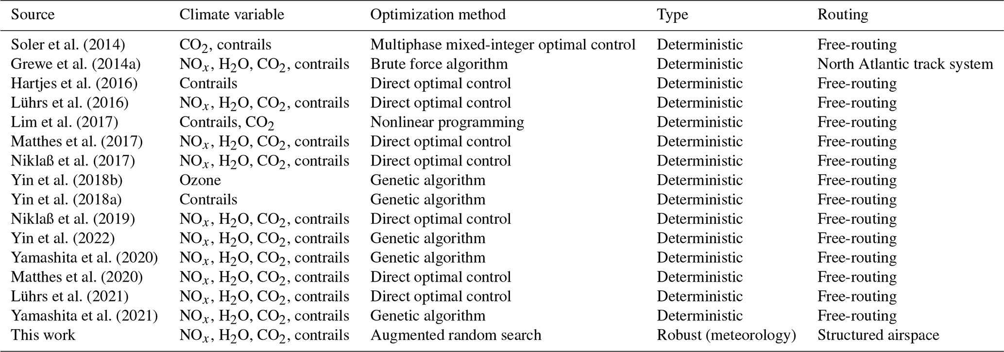
As for climate-optimal trajectory planning methods, various strategies ranging from mathematical programming (e.g., Campbell et al., 2008) to meta-heuristic (e.g., Yin et al., 2018a; Yamashita et al., 2020), indirect optimal control (e.g., Sridhar et al., 2011), and direct optimal control methods (e.g., Niklaß et al., 2017; Lührs et al., 2021, 2016; Matthes et al., 2020) have been adopted. For instance, the direct optimal control approach has been employed by Hartjes et al. (2016) to minimize flight time (or distance flown) in areas sensitive to persistent contrail formation, by Lührs et al. (2021) to minimize average temperature response over the next 20 years (ATR20) associated with non-CO2 emissions, and by Vitali et al. (2021) to minimize the global warming potential (GWP) of NOx, H2O, soot, SO2, and contrails. Using aCCFs to quantify climate impacts, Yamashita et al. employed a genetic algorithm to determine climate-optimal aircraft trajectories (Yamashita et al., 2020, 2021). Regarding the optimization methodologies, the mathematical programming methods only apply to simplified aircraft trajectory optimization problems (e.g., in the study conducted by Campbell et al., 2008, the aircraft's dynamic behavior is represented with a linearized model). The meta-heuristic methods (e.g., genetic algorithm) require very fast aircraft trajectory prediction in order to find an optimal solution with a large number of iterations; thus, the flight planning problem is usually approximated with a simplified but representative enough problem (e.g., in Yamashita et al., 2020, the optimization is defined with 11 decision variables to characterize lateral path and flight altitude, and the speed profile is considered constant). Finally, with the optimal control methods, the capability to model more accurate aircraft trajectory optimization problems is provided since the problem is represented as a dynamic optimization problem. Nevertheless, there are some drawbacks associated with addressing the formulated problem. The dynamic programming method (as an optimal control approach) results in the “curse of dimensionality” for complex problems (e.g., a full 4D aircraft trajectory optimization problem). Regarding the indirect optimal control approach, deriving analytical solutions using Pontryagin's maximum principle is daunting, especially for problems with singularities (e.g., only a 2D trajectory optimization problem has been addressed in the literature; Sridhar et al., 2011). The direct optimal control approach, despite being very flexible in modeling aircraft trajectory optimization problems (e.g., considering a full 4D dynamical model with nonlinear path and boundary constraints; Lührs et al., 2021), has a high sensitivity to initial conditions, and thus local optimality is its main drawback. In addition, considering the airspace structure with indirect and direct optimal control methods is not straightforward. Interested readers are referred to Simorgh et al. (2022) for our recent comprehensive survey on climate-optimal aircraft trajectory planning, reviewing both the approaches to model climate-sensitive regions and trajectory planning methods. A classification of the most recent studies in this field is provided in Table 1.
To quantify the non-CO2 climate effects, specific weather variables are required. In the case of aCCFs, variables such as temperature (T), potential vorticity (PV), geopotential (Φ), relative humidity over ice (rhum), and outgoing longwave radiation (OLR) are needed. These variables are obtained from standard weather forecasts. Several factors, including incomplete understanding of the state of the atmosphere, computational complexity, and nonlinear and sometimes chaotic dynamics, affect the accuracy of weather predictions, implying that the weather forecast is inevitably uncertain (WMO, 2012). These weather-forecast-related uncertainties in the aCCFs and also in aircraft dynamical behavior (e.g., uncertainty in wind and temperature), if not accounted for within aircraft trajectory planning, can lead to inefficient trajectories. Previous research in the field of climate-optimal aircraft trajectory planning has been conducted in a deterministic manner, neglecting the inclusion of any sources of uncertainty (see Table 1) (Simorgh et al., 2022). A first step in managing and integrating meteorological uncertainties into aircraft path planning is to obtain reliable weather forecasts that can predict probable variations in meteorological conditions. To characterize weather forecast uncertainties, probabilistic weather forecasting (PWF) is typically used (AMS-Council, 2008). State-of-the-art probabilistic weather forecasting is obtained from the ensemble prediction system (EPS), which provides NEPS possible realizations of meteorological conditions called ensemble members (Bauer et al., 2015).
When accounting for the ensemble weather forecast in solving aircraft trajectory optimization, the computational time is an important issue that arises in addition to the capability to consider such uncertainties. This is due to the fact that, instead of taking one weather forecast and solving the trajectory optimization in a deterministic manner, the optimizer should be capable of considering NEPS (e.g., NEPS=50) different forecasts. Several studies have been proposed in the literature to determine robust aircraft trajectories in the presence of meteorological uncertainty quantified using EPS weather forecast (though not considering climate impact; Simorgh et al., 2022). However, these studies suffer mainly from computational perspectives (i.e., the computational time of the optimizer when considering weather uncertainty) and some restrictive assumptions (e.g., inaccurate modeling of the aircraft dynamical model or ignoring important decision variables such as the flight altitude) (Simorgh et al., 2022, Sect. 5.3). For instance, in the study conducted by González-Arribas et al. (2018), a robust aircraft trajectory optimization problem is solved using the optimal control approach within fully free-routing airspace. In this approach, the effects of uncertainty are included in the optimization problem by expanding the dynamical model of the aircraft (almost) linearly to the number of ensemble members, resulting in a larger dimensional deterministic optimization problem. Thus, it requires more computational time compared to the deterministic flight planning problem. Also, the flight planning problem is limited to optimizing only the lateral path. As for the structured airspace, Franco Espín et al. (2018) proposed uncertain flight plan optimization using mixed-integer linear programming (MILP). Similarly, the optimization in this study is performed in 2D airspace. In addition, the fuel burn and its associated nonlinearities are ignored, and it has a sizable computational cost of several minutes. In this respect, developing efficient trajectory optimization solvers capable of delivering robust climate-optimal trajectories with a computational time compatible with operations has been identified as a scientific gap (see Simorgh et al., 2022).
The focus of recent studies has been restricted to planning climate-optimal trajectories considering the concept of future free-route airspace (see last column Table 1), which is thus not applicable for the structured airspace of today. The trajectory optimization problem constrained by the structure of airspace results in hybrid decision spaces (e.g., route and flight level are discrete, and speed schedule is continuous) (González-Arribas et al., 2023). The trajectory optimization problem with the combination of discrete and continuous decision variables is one of the most challenging optimization problems, typically solved using mixed-integer nonlinear programming with intensive computational cost (see, e.g., Bonami et al., 2013).
Soler et al. (2014)Grewe et al. (2014a)Hartjes et al. (2016)Lührs et al. (2016)Lim et al. (2017)Matthes et al. (2017)Niklaß et al. (2017)Yin et al. (2018b)Yin et al. (2018a)Niklaß et al. (2019)Yin et al. (2022)Yamashita et al. (2020)Matthes et al. (2020)Lührs et al. (2021)Yamashita et al. (2021)Table 1A classification of the recent studies in the literature proposed to reduce the climate impact of aircraft emissions with aircraft trajectory optimization.
Drawing upon the brief literature review and the presented open problems, we aim to address the problem of determining robust climate-optimal aircraft trajectories within the structured airspace in this study. Our main contributions are summarized as follows: (1) full 4D climate-optimal trajectory planning within the currently structured airspace, (2) accounting for uncertain meteorological conditions and uncertainty associated with initial flight conditions such as departure time and aircraft initial mass, and (3) determining the optimized trajectory computationally very fast. The uncertainty in weather forecast is characterized using the ensemble prediction system, and aviation's climate impacts are quantified by employing the latest version of aCCFs (V1.0A). The concept of robustness that we refer to is the determination of the aircraft trajectory considering all possible realizations of meteorological variables provided using an EPS weather forecast. In other words, instead of planning a trajectory based on one forecast in a deterministic manner, we aim to determine a trajectory that is optimal considering the overall performance obtained from using different members of an ensemble weather forecast. In this respect, from the operational point of view, the optimized trajectory is tracked as determined, and the effects of meteorological uncertainties are reflected in the flight performance variables such as flight time, fuel burn, and climate impact. Mathematically, the perturbations due to the meteorological uncertainty are considered in the dynamical model of aircraft, and the proposed trajectory optimization is generic in terms of the objective function, in which a wide range of objectives, such as flight time, fuel consumption, emissions, and climate impact, and different statistics including expected values and variance of the performance variables, can be considered. Such flexibility in defining the cost function allows for solving a multi-objective optimization problem. Moreover, by penalizing the mean and variance of the objectives, the effects of uncertainty on flight variables can be controlled. In this study, the flight planning objective is a weighted sum of the simple operating cost (as a function of flight time and fuel consumption) and climate impact. The focus is restricted to optimizing the expected performance since, as will be shown in the simulation results, minimizing the averaged performance leads to reducing the uncertainty ranges for the considered case studies.
We employ the probabilistic flight planning method firstly developed by González-Arribas et al. (2023) to determine robust climate-optimal trajectories for three phases: climb, cruise, and descent. In this approach, to account for discrete and continuous decision variables in an integrated manner, the optimization is carried out on the space of probability distributions defined over flight plans instead of directly searching for the optimal profile. Then, the probability distribution over flight plans is parameterized, allowing the generation of multiple flight plans stochastically. The augmented random search algorithm is employed and implemented on graphics processing units (GPUs) to deliver a nearly optimal solution to the resulting stochastic optimization in seconds. We have developed an open-source Python library called ROOST V1.0 (Robust Optimization of Structured Trajectories) based on the proposed robust aircraft trajectory optimization technique, which is currently available via the DOI https://doi.org/10.5281/zenodo.7121862 (Simorgh, 2022). ROOST is a tool that efficiently uses the information provided by the prototype aCCFs (implemented in our recently developed Python library CLIMaCCF V1.0 (DOI: https://doi.org/10.5281/zenodo.6977273; Dietmüller et al., 2022) for planning climate-optimal trajectories accounting for the operational constraints and uncertainty. It should be noted that CLIMaCCF V1.0 is the first release of the Python library, which includes both versions of aCCFs, i.e., V1.0 and V1.0A. For performing aircraft trajectory optimization in this study, we use V1.0A aCCFs. Users need to input the required weather variables, route graphs, and aircraft type specifications to start working with the library. In addition, users should assign values to the weighting parameters associated with different objectives in the objective functions. This paper is mainly devoted to the climate-optimal aircraft trajectory planning algorithm implemented in the library and its application to optimize different case studies. Instructions to get started with the library can be found in the repository of ROOST.
The paper is arranged as follows. The robust climate-optimal aircraft trajectory planning problem is stated and formulated in Sect. 2 and solved in Sect. 3. The potential of our flight planning algorithm to reduce aviation-induced climate impacts under uncertain meteorological conditions is explored in Sect. 4. Finally, the discussion on the obtained results and concluding remarks are presented in Sect. 5.
Aviation-induced non-CO2 climate effects have a direct dependency on atmospheric conditions at the location and time of emissions. In this respect, generating flight plans that could potentially minimize emissions in areas with high sensitivity to aircraft emissions in terms of climate change is a step towards climate-friendly air transport. To enable such a flight planning strategy, information on climate-sensitive areas is required first. Once climate information is available, it needs to be included in flight planning tools to generate eco-efficient trajectories. It is worth mentioning that to generate reliable trajectories, different sources of uncertainty need to be identified, understood, and quantified.
The focus of this study is on determining robust flight plans taking into account meteorological uncertainty and uncertainty associated with the initial flight conditions. In this respect, we start by presenting a general formulation of the dynamic optimization problem with uncertainty in Sect. 2.1, which is then employed to model the proposed robust flight planning (in Sect. 2.2). In Sect. 2.3, the effects of meteorological uncertainty on the efficiency of climate-optimal trajectories are discussed, and the motivation to solve robust trajectory optimization is provided.
2.1 General formulation of dynamic optimization problem with uncertainty
We present a general formulation of a dynamic optimization problem with the inclusion of uncertainty effects, focusing mainly on the dynamical model and objective function.
Let us consider a class of dynamical systems with uncertainty as follows:
where , , and are the vectors of control inputs as well as states and algebraic variables, respectively, and f is a vector field, mapping . The uncertain parameters (denoted with ) are considered continuous random variables and assumed to have known probability distribution functions , where Ω is a space of possible outcomes. The random variables take different values depending on the probable outcomes (i.e., ζ(ω) for ω∈Ω). The nonlinear function f(⋅) is assumed to be a measurable function in ζ. To emphasize the effects of random variables on the system's trajectories, all the variables were denoted with dependency on possible outcomes (e.g., x(t,ω)). For the sake of improving clarity, the abbreviated notation (e.g., x(t)) will be used in the following.
A general form of the cost functional considered for dynamic optimization problems with uncertainty is
where and are the Mayer and Lagrangian terms, respectively. Notice that the objective function and also dynamical model are similar to what is usually considered within the context of optimal control theory. Although the objective function is written in terms of using the expectation operator, other statistics can be evaluated under this formulation. For instance, one can include the variance of a function A(ζ) as , where 𝕍{⋅} is the variance operator. Depending on the benchmark problem, several constraints such as equality and inequality path and boundary constraints are considered (see Simorgh et al., 2022).
The objective of the stated dynamic optimization problem is to find a feasible control policy (u∈𝒰) to minimize the performance index (Eq. 2) respecting a set of constraints, including dynamical constraints (Eq. 1). Depending on the benchmark problem, reformulations and approximations are normally made to address the required performance, such as computational complexity. In this study, we will slightly reformulate the optimization for the proposed path planning problem.
2.2 Robust climate-optimal flight planning problem formulation
The definition of the aircraft trajectory optimization problem mainly requires the aircraft dynamical model, flight planning objectives, and physical and operational constraints. To consider climate impact within aircraft trajectory planning, information on the climate impacts of CO2 and non-CO2 emissions is necessary and needs to be included in the objective function. In the following, the modeling of the mentioned elements is briefly presented.
2.2.1 Aircraft dynamical model
To determine reliable aircraft trajectories, accurate aircraft dynamical models are necessary. In this work, the point-mass model with the following equations of motion is used to represent the aircraft's dynamical behavior, as is usually considered within air traffic management studies.
Here, ϕ is the latitude, λ is the longitude, v is the true airspeed, h is the altitude, m is the mass, CT is the thrust coefficient, γ is the climb angle, χ is the heading angle, , and (wx,wy) are wind components. The Earth's ellipsoid radii of curvature in the meridian and the prime vertical are denoted with RM and RN, respectively, T is the magnitude thrust force, and the drag force is denoted with D. g is the Earth's gravity, FF is the fuel flow, and S is the wetted surface of the aircraft. The BADA4.2 model (Gallo et al., 2006) is employed to provide the aerodynamic and propulsive performance of the aircraft. Notice that we used the notation presented in Sect. 2.1 (i.e., ω) to represent the uncertainty in the temperature and components of wind. The realization of the state and control variables depends on uncertainty, e.g., for mass, ; in the interest of notational clarity, we use the abbreviated notation m.
Structured airspace
As trajectory optimization in this study is performed within the structured airspace, the evolutions of aircraft states are constrained. In the following, we briefly present our proposed modeling of airspace structure and flight plan.
We consider a directed acyclic graph to model the airspace with V as the navigation waypoints and e∈E as the airway edges connecting waypoints. The trajectory is assumed to start at the end of the standard instrument departure procedure (SID) and end at the beginning of the standard instrument arrival procedure (STAR) to the destination airport, denoted as o∈V and d∈V, respectively. We define the flight plan ℱ with a tuple . In the flight plan (ℱ), the route (or lateral path) denoted as ℛ includes a sequence of waypoints, i.e., . The vertical profile of the cruise, , is composed of an ordered sequence of tuples of the form (rk,FLk), indicating that, if the aircraft is in the cruise phase, the flight level will be changed to FLk when the waypoint rk is reached (see Fig. 1). The Mach schedule indicates the target Mach number Mk at waypoint rk during the cruise phase. Climb and descent profiles are represented by continuous and piecewise-differentiable functions mapping the altitude to the target airspeed during the climb and descent phases, respectively. Finally, a scalar variable d𝒟 shows the distance to go to the destination node at which the aircraft should end the cruise and start the descent phase.
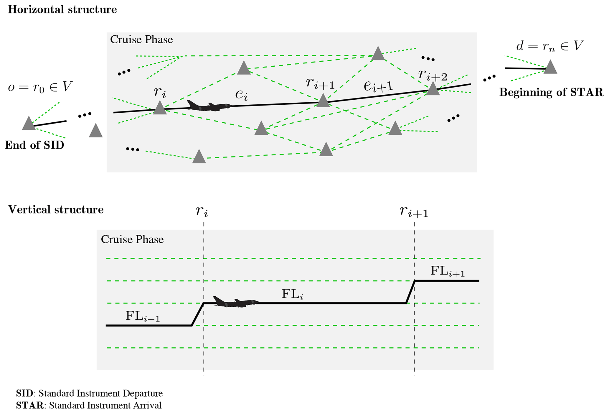
Figure 1Structure of airspace. The route graph is generated by processing the full airspace graph to include paths from the end of the SID to the beginning of the STAR to the destination airport.
2.2.2 Objective function
The goals of the aircraft trajectory optimization problem are interpreted mathematically and defined as an objective function to be minimized (or maximized). In addition to the climate impact, the operating cost is a crucial aspect that needs to be considered as it is one of the main interests of airliners. Generally, there is a trade-off between the operating cost and climate impacts. This is due to the fact that rerouting areas sensitive to climate increases operational costs as the aircraft tends to fly longer routes (Niklaß et al., 2021). To consider both objectives in the trajectory optimization, we define the following objective function:
where ψCST and ψCLM are weighting parameters penalizing cost and climate impact, respectively. In the following, the proposed modeling of these two objectives is presented.
Operating cost
There are various approaches to account for operating costs within aircraft path planning. Flight time and/or fuel are common objectives. However, more realistic cost metrics exist, which include additional costs such as flight crew, cabin crew, and landing fees. Interested readers are referred to Simorgh et al. (2022) for a classification of these metrics.
In this study, we use simple operating cost (SOC) as a metric expressing cost in USD with linear relation to flight time and fuel consumption:
where t0 and tf are the initial flight time and final flight time weighted by ψt=0.75 USD s−1, and m0 and mf are the initial mass and final mass weighted by ψm=0.51 [USD kg−1]. The expectation operator is used here because the meteorological uncertainty (included in the aircraft dynamical model) and also uncertainty due to initial conditions directly affect the flight time and fuel consumption.
In spite of considering only flight time and fuel consumption to represent the operating cost, it was reported in Table 4 of Yamashita et al. (2020) that employing SOC and a more comprehensive metric such as cash operating cost within trajectory optimization delivered almost similar results. This is because these two metrics, in the end, consider flight time and fuel consumption as inputs to estimate the operating cost.
Climate effects induced by aviation
Numerous approaches have been proposed in the literature to consider climate impact within aircraft trajectory planning strategies (see Table 1 and Fig. 2 of Simorgh et al., 2022). In this study, the climate impact of aircraft operations is modeled using the prototype aCCFs. These aCCFs take as input specific meteorological variables (e.g., temperature and relative humidity) and estimate the climate impact in terms of average temperature change. The suitability of aCCFs for climate-optimal trajectory planning can be justified as follows:
-
aCCFs account for the temporal and spatial dependency of climate impacts associated with non-CO2 species, including ozone and methane, resulting from NOx emissions, water vapor emissions, and persistent contrails;
-
aCCFs estimate the climate impact associated with aircraft emissions computationally in real time, making it well-suited for climate-optimal trajectory planning; and
-
aCCFs directly quantify climate impacts in average temperature change.
The aCCF V1.0 reported by Yin et al. (2022) is the first complete and consistent set of prototype aCCFs providing spatially and temporally dependent non-CO2 climate effects in terms of average temperature response over the next 20 years for a pulse emission scenario (P-ATR20). In this study, we use the latest version of aCCFs, i.e., aCCF V1.0A developed by Matthes et al. (2023) within the EU project FlyATM4E, which has been calibrated to the state-of-the-art climate response model AirClim (Dahlmann et al., 2016).
The V1.0A aCCFs are multiplied by some factors in order to be more suitable for the flight planning application.
-
Metric conversion. The selection of a suitable metric depends on the question to be answered (see Grewe and Dahlmann, 2015, for more details); therefore, different questions require the use of different metrics. The P-ATR20 metric was selected as a metric for the aCCFs to assess the impact of a “simple” pulse emission. However, factors are available (see Dietmüller et al., 2022) to convert P-ATR20 to other metrics: for example, assuming the future emission scenario or longer time horizons. This way, one can select the emission scenario and time horizon that are best-suited for the question. In this study, the F-ATR20 metric is used to assess the climate effect reduction obtained by steadily applying a specific routing strategy under the assumption of a future business-as-usual emission scenario. To this end, the aCCFs based on the pulse emission scenario are converted to the future scenario (F-ATR20) using values reported in Table 3 of Dietmüller et al. (2022). These conversion factors were derived by simulations with the climate response model AirClim (Dahlmann et al., 2016): one simulation with pulse emission and one with the future emission scenario. By comparing the two simulations, the factors can be derived.
-
Efficacy. Efficacies were introduced to take into account the fact that the radiative forcing of some non-CO2 forcing agents (e.g., ozone, methane, contrails) is more or less effective in changing the global mean near-surface temperature per unit forcing compared to the response of CO2 forcing (Hansen et al., 2005; Ponater et al., 2007). Dietmüller et al. (2022) have summarized the efficacy parameters reported by Lee et al. (2021). For a detailed explanation of efficacy, the reader is referred to the state-of-the-art literature (e.g., Ponater et al., 2007; Rap et al., 2010; Bickel et al., 2020).
For the sake of compactness of notation, F-ATR20 (from aCCF V1.0A) with efficacy parameters is replaced with ATR in the following.
For the aCCFs of (daytime and nighttime) contrails, the ice supersaturation is applied using temperature and relative humidity over ice in order to predict regions where persistent contrails are expected to form, called persistent contrail formation areas (PCFAs) (Schmidt, 1941; Appleman, 1953). To represent the climate impacts using aCCFs in the average temperature change (i.e., [K]), fuel consumption rate, NOx emissions, and distance flown through PCFAs are required.
The geographical aCCF pattern of water vapor, NOx-induced ozone (production), and methane (destruction), as well as of contrails, is shown in Fig. 2a–c for 13 June 2018 at 00:00 UTC over the European region for FL340. Moreover, Fig. 2d shows the pattern of the merged non-CO2 aCCFs that combines the individual aCCFs (Fig. 2a–c). Note that to generate the merged aCCFs and to compare the contribution of each species, we adopt typical transatlantic fleet mean values to unify the units of aCCFs in K kg−1(fuel). The approximated conversion factors for NOx emissions and contrails are kg(NO2) kg−1(fuel) and 0.16 km kg−1(fuel), respectively (Graver and Rutherford, 2018; Penner et al., 1999). It is clear from the merged aCCFs that the contrails have dominant climate effects, which is in line with related studies employing aCCFs (see, e.g., Dietmüller et al., 2022).
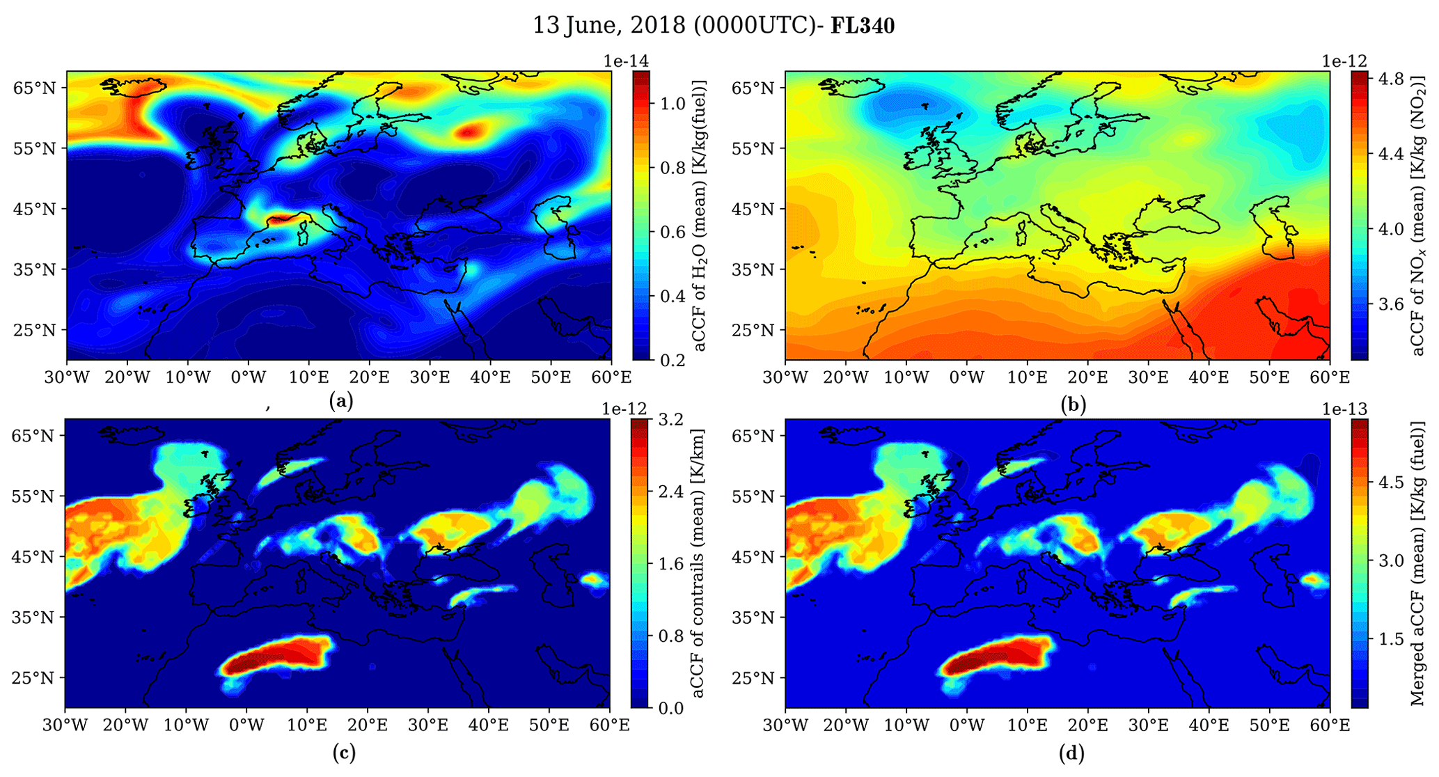
Figure 2Algorithmic climate change functions of (a) water vapor, (b) NOx, (c) contrails, and (d) the total non-CO2 effects on 13 June 2018 at 00:00 UTC over European airspace for FL340.
To benefit from the spatial and temporal dependency of non-CO2 climate effects identified using aCCFs in planning climate-optimal trajectories, we define the following objective expressed in the Lagrangian form for Eq. (4).
for :
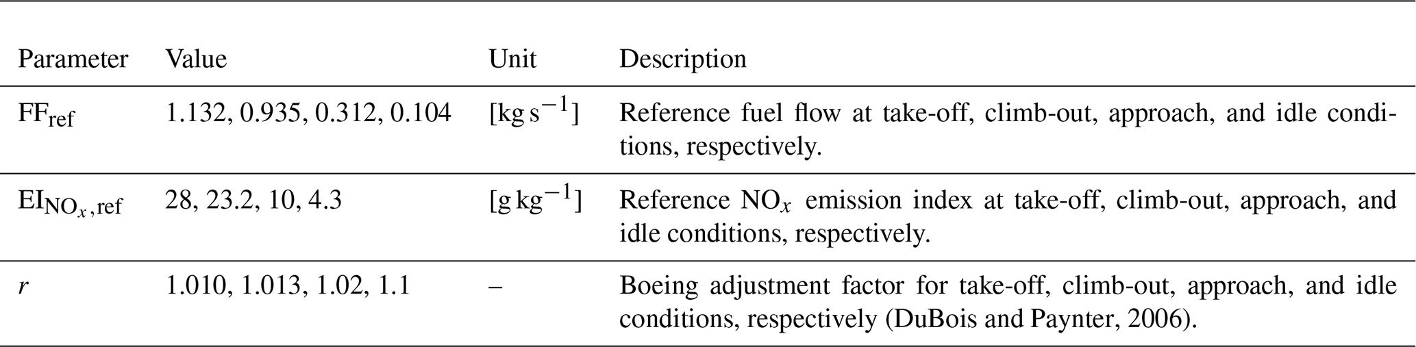
Here, is a vector of uncertain variables, i.e., meteorological variables and initial flight conditions. In addition, , where is the actual NOx emission index in [g(NO2) kg−1(fuel)], and vgs is the ground speed. The NOx emission index varies with many factors such as aircraft type, fuel flow, flight altitude, and synoptical situation. To consider such dependencies, the Boeing fuel flow method 2 (BFFM2), calculating the actual emission index of NOx from the reference conditions, is adopted (DuBois and Paynter, 2006; Jelinek, 2004). The reference conditions are obtained from the International Civil Aviation Organization (ICAO) data bank (https://www.easa.europa.eu/en/domains/environment/icao-aircraft-engine-emissions-databank, last access: 2 July 2023). Notice that the objective regarding climate impact is expressed in the Lagrangian form (i.e., as an integral) since the climate impact needs to be evaluated (and accumulated) along the route, unlike the operating cost, which requires only information on boundary values (e.g., initial and final flight time). Notice that we define the objectives considering the expected performance. One can use other statistics, such as variance, without loss of generality. For instance, to penalize the range of uncertainty in climate impacts, should be included in the objective function. For the considered case studies, it will be shown that minimizing the expected objective function will reduce the uncertainty in the most uncertain variable for the climate-optimal routing option, thus providing a robust solution without penalizing the deviation.
2.3 Effects of weather-induced uncertainty on climate
The dynamical model of aircraft requires weather-related variables such as wind and temperature (see, e.g., Sect. 2.2.1). In addition, the non-CO2 climate effects of aviation included in the objective function of the optimization problem strongly rely on weather conditions. Since the required meteorological variables are obtained from standard weather forecasts, they are inevitably uncertain. It is worth mentioning that there are other sources of uncertainty affecting the efficiency of the planned climate-optimized trajectories, including uncertainty from climate science (e.g., modeling and estimating aviation-induced climate effects), emission calculation, and also inaccurate modeling of aircraft behavior, which are not within the scope of this paper but have been identified as open problems (see Matthes et al., 2023).
In this paper, the focus is on forecast-related uncertainties, which will be characterized by employing ensemble prediction system (EPS) weather forecasts, a numerical weather prediction method introduced to deal with uncertainty in weather forecast (Bauer et al., 2015). These are forecasts in which both the initial conditions and the physical parameters of a numerical weather integration model are slightly modified from one member to another and provide NEPS (typically NEPS = 50) different predictions known as ensemble members (Bauer et al., 2015). Each member of an ensemble represents one possible realization of meteorological situations. As the aCCFs take as inputs some meteorological variables, NEPS different aCCFs can be calculated for an EPS weather forecast. For instance, the meteorological variables temperature and relative humidity over ice are required for the aCCF of nighttime contrails. Notice that relative humidity over ice is required for identifying ice-supersaturated areas. Feeding NEPS probable realizations of these meteorological variables (i.e., ensemble members), NEPS different aCCFs (i.e., for ) are calculated. The same applies to system dynamics (considering uncertainty in temperature and wind) and also the NOx emission index (due to the dependency on ambient temperature and specific humidity).
To investigate the degree of uncertainty (or variability) in the meteorological variables provided by an EPS and its effects on the computed aCCFs, we take the standard deviation (SD) from 10 ensemble members of weather data obtained using the ERA5 reanalysis data products (https://cds.climate.copernicus.eu/, last access: 2 July 2023). It should be noted that the reanalysis data products are generated from post-processing with observations. Thus, the variability among the ensemble members is expected to be lower than the forecast data with more ensemble members yet still valid to illustrate. Figure 3 shows the SD of weather variables required to calculate the aCCFs and aircraft trajectory on 13 June 2018 at 00:00 UTC for FL340. The SD is taken over the normalized variables (with respect to their maximum values) for comparison purposes. The variability of geopotential, temperature, and wind is small compared to potential vorticity, outgoing longwave radiation, and relative humidity. The SDs of the calculated aCCFs based on the ensemble members are illustrated in Fig. 4. Since the aCCF of NOx emissions (i.e., methane and ozone) depends on geopotential and temperature, its SD is small compared to the aCCFs of water vapor and nighttime contrails, which are based on potential vorticity and relative humidity (when applying the ice-supersaturated condition), respectively. Notice that the uncertainty in the climate impact of contrails is much higher than water vapor due to the variability of relative humidity in satisfying the persistency condition of contrails (see SD of PCFA in Fig. 4). Due to the considered time (i.e., 00:00 UTC), the aCCF of contrails is based on the formulation of nighttime aCCFs. In spite of negligible uncertainty in the aCCF of NOx and also relatively low uncertainty in the aCCF of water vapor compared to aCCF of contrails, due to the dominant climate impact of contrails, the net non-CO2 climate effect is considerably uncertain (see SD of the merged aCCFs in Fig. 4), which must be crucially taken into consideration.
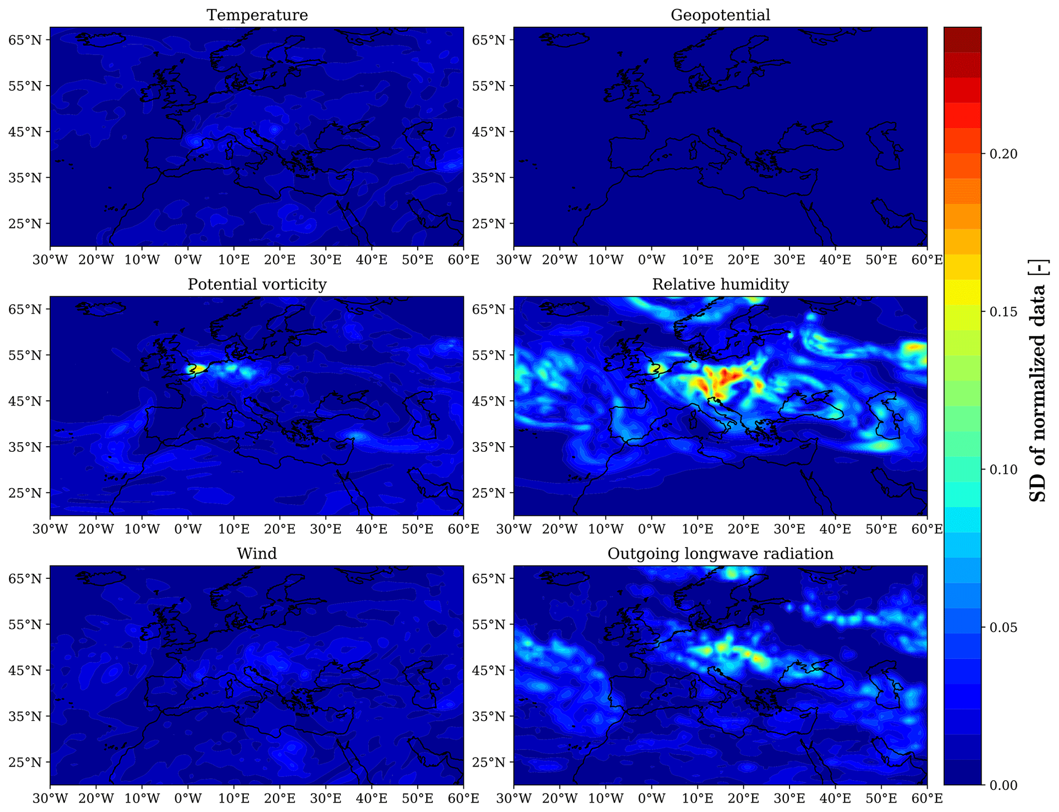
Figure 3Variability (quantified using SD) of the meteorological conditions for an ensemble weather forecast with 10 ensemble members on 13 June 2018 at 00:00 UTC over European airspace for FL340.
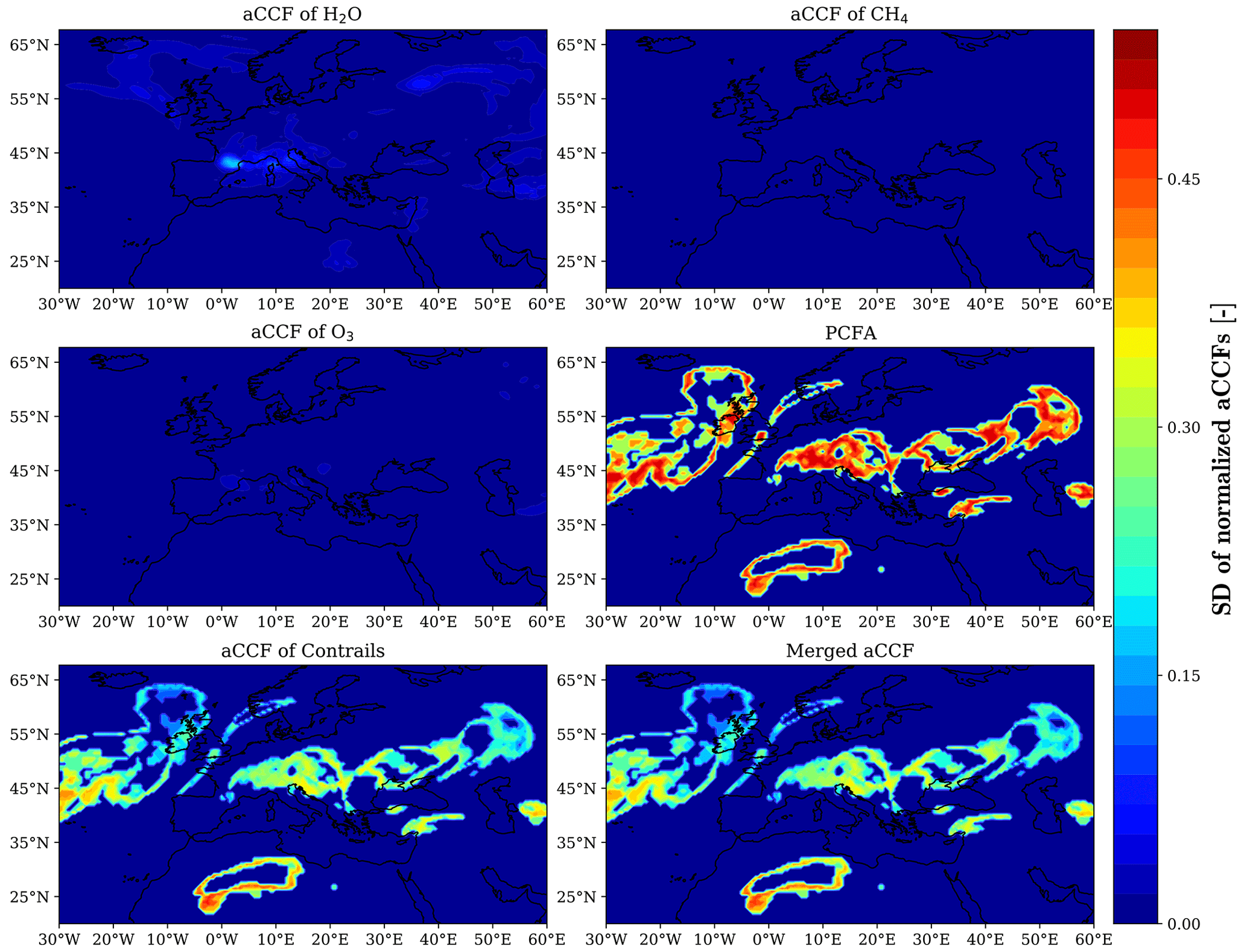
Figure 4Variability (quantified using SD) of aCCFs for an ensemble weather forecast with 10 ensemble members on 13 June 2018 at 00:00 UTC over European airspace for FL340.
Figure 5 shows how uncertainty in meteorological variables can affect the performance of aircraft trajectories. As can be seen, these uncertainties are accumulated and can considerably degrade the efficiency of the optimized trajectory if not considered in the aircraft trajectory planning a priori. No recent study on the determination of climate-optimized trajectories has considered robustness in the sense of uncertainty in weather forecasts. One of the main reasons for not considering such variations is the computational time that arises within the optimization techniques. In fact, instead of considering one member, the optimization, in this case, is to consider NEPS ensemble members (e.g., 50) and find an optimized trajectory to be optimal with respect to all probable realizations of meteorological variables. Such an increase in dimensions is daunting to cope with by employing classical dynamic optimization approaches such as direct optimal control.
In Sect. 3, we will address the problem of robust climate-optimal trajectory planning with an efficient heuristic method implemented on GPUs.
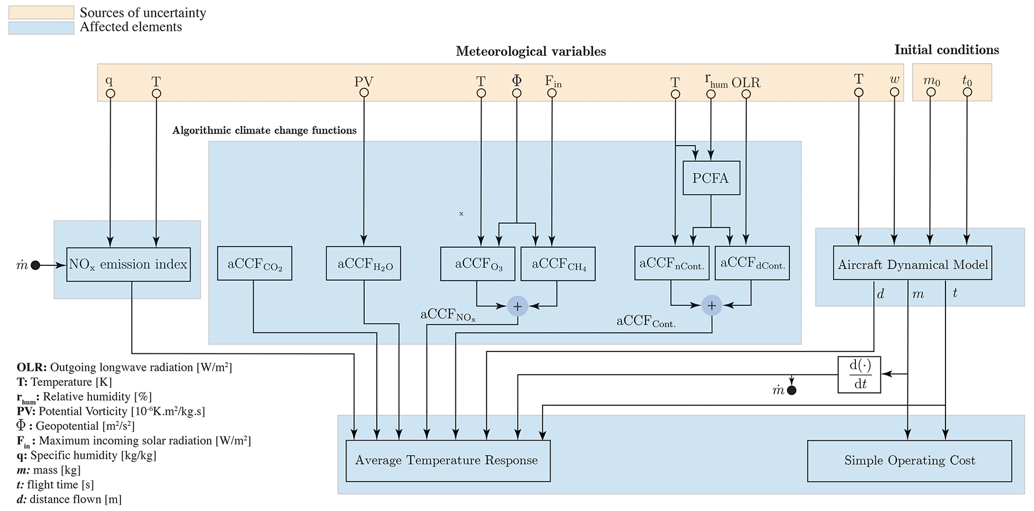
Figure 5Propagation of uncertainties (associated with initial flight conditions and meteorological variables) within climate-optimal aircraft trajectory planning.
The aircraft trajectory optimization problem formulated in Sect. 2.2 is solved by employing the method firstly developed by González-Arribas et al. (2023), which is a heuristic optimization technique for the structured airspace and is capable of determining the optimized trajectory in four dimensions, i.e., latitude, longitude, altitude, and time.
As mentioned in Sect. 2.1, depending on the problem, some reformulations and approximations are normally made to the dynamic optimization problem to address the required objectives. Here, instead of seeking the optimal control policy (i.e., uo), the goal is to find an optimal flight plan ℱo, i.e., (see Sect. 2.2.1) that minimizes the objective function given in Eq. (4) and satisfies the aircraft dynamical model (given in Eq. 3), airspace structure, and path and boundary constraints. Such a selection of decision space allows us to directly account for the operational restrictions, such as determining lateral routes that follow the airspace structure.
3.1 Ensemble trajectory integration
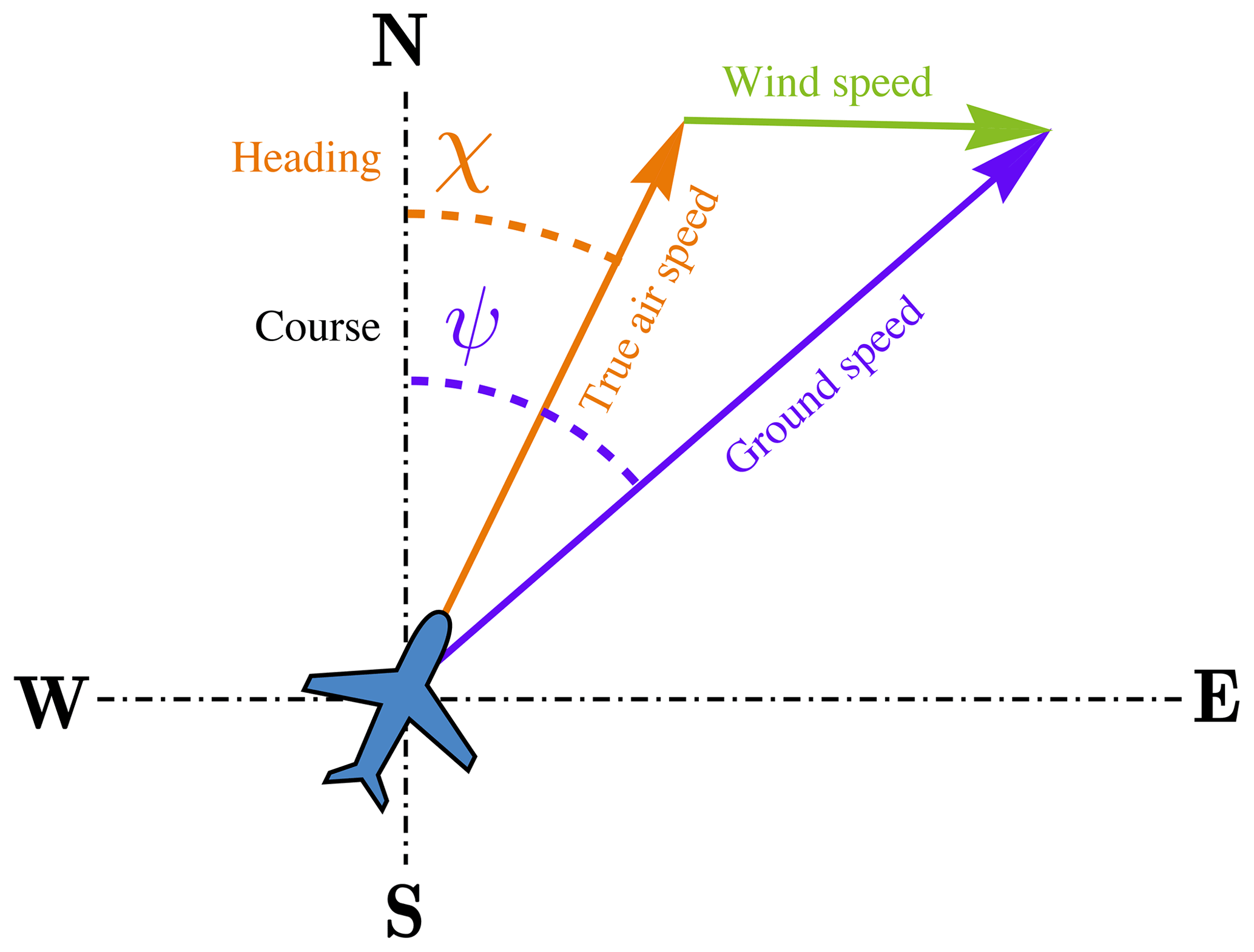
To determine the performance of a flight plan and evaluate the cost function Eq. (4), the corresponding trajectories of the aircraft are to be calculated using the aircraft dynamical model (provided in Sect. 2.2.1). As mentioned in Sect. 2.3, aircraft trajectories are affected by uncertainty in meteorological variables, including temperature and wind. Assuming a unique lateral path (constant course) to be tracked in practice with low-level controllers in real time, the uncertainty in the wind (both magnitude and direction) will affect ground speed and, consequently, the time the aircraft flies the route (see Fig. 6). In addition, uncertainty in temperature affects fuel consumption because the propulsive and aerodynamic performance of the aircraft and also airspeed have a dependency on temperature (González-Arribas et al., 2023). From Eq. (6), one can conclude that the uncertainty in flight time and flight mass can also affect the climate impacts (see also Fig. 5). In addition to the uncertainty in meteorological variables, which is characterized using ensemble weather forecasts, uncertainty associated with initial flight conditions is taken into account within the trajectory optimization problem. In this study, the initial flight time and initial mass of the aircraft are modeled as Gaussian variables, i.e., and .
To efficiently reflect the effects of wind uncertainty in flight performance variables, instead of time, the distance flown along the route (s) is considered to be the independent variable using . This is beneficial since the uniqueness of time for all possible realizations of wind means that the position of the aircraft is fixed with respect to time. In this case, the effects of uncertainty cannot be considered efficiently because the range of feasible solutions is limited. The selection of distance flown as the independent variable allows for reflecting wind uncertainty in flight time.
According to the defined objective function (Eqs. 4, 5, 6), the flight performance variables required to evaluate Eq. (4) are flight time, final mass, and climate impact. By using TI(⋅) to denote the integration of the aircraft dynamical model for a given flight plan, weather data, and initial flight conditions, we receive the expected final mass, the expected final time, and the expected ATR required to evaluate the performance of aircraft trajectory (i.e., calculate the objective function given in Eq. 4) as follows:
In the formulated robust optimization problem, the uncertain variables are considered to be continuous random variables with known probability distribution functions. As the weather variables for an ensemble weather forecast are directly represented in a discrete fashion, we assume a discrete probability distribution for the uncertainty. Considering NEPS probable realizations of uncertainty (i.e., ), we have
where 𝒲j(⋅) is a set of meteorological variables required for climate-optimal aircraft trajectory planning corresponding to the jth member of an EPS weather forecast, and , and m0 are initial flight conditions that are sampled independently. Generally, different members of the ensemble weather forecasts are considered equally probable. This implies that a specific forecasted weather pattern that has a higher probability will be represented by a larger number of ensemble members. In this study, we use equal weights for each probable realization of weather variables, i.e., with a probability of . Thus, using an unweighted average between all ensemble members, Eq. (8) can be written as
The expected ATR is calculated as
for . For instance, ATRj for ozone and contrails can be calculated as
where xj(tj) and uj(tj) are the state and control variables of the aircraft considering the jth realization of weather variables and the jth sampled initial conditions, , and
where weather variables such as Tj and Φj are the jth members of the ensemble weather forecast. The actual NOx emission index, i.e., , is calculated using BFFM2. As can be seen in Eq. (11), the climate impact due to the NOx emissions depends on the amount of NOx emitted in NOx-sensitive regions (i.e., multiplied by the aCCF of NOx emissions), while for contrails, it depends on the distance flown in persistent contrail formation areas.
Heun's method is adopted for integrating the aircraft dynamical model along discretized segments of the route through each phase, i.e., climb, descent, and cruise (González-Arribas et al., 2023). Since the calculations are similar for different members, parallelization would be beneficial in reducing computational time. Here, CUDA (Guide, 2013; Klöckner et al., 2012), a tool for general-purpose computing on the graphics processing unit, is employed to parallelize the computations.
3.2 Performance evaluation of a flight plan
The expected values obtained from Eq. (10) are for a specific flight plan. By these settings, for this flight plan, the cost function given in Eq. (4) can be evaluated with the following equation:
Figure 7 shows how the expected performance is calculated and evaluated for a given flight plan and an ensemble weather forecast.
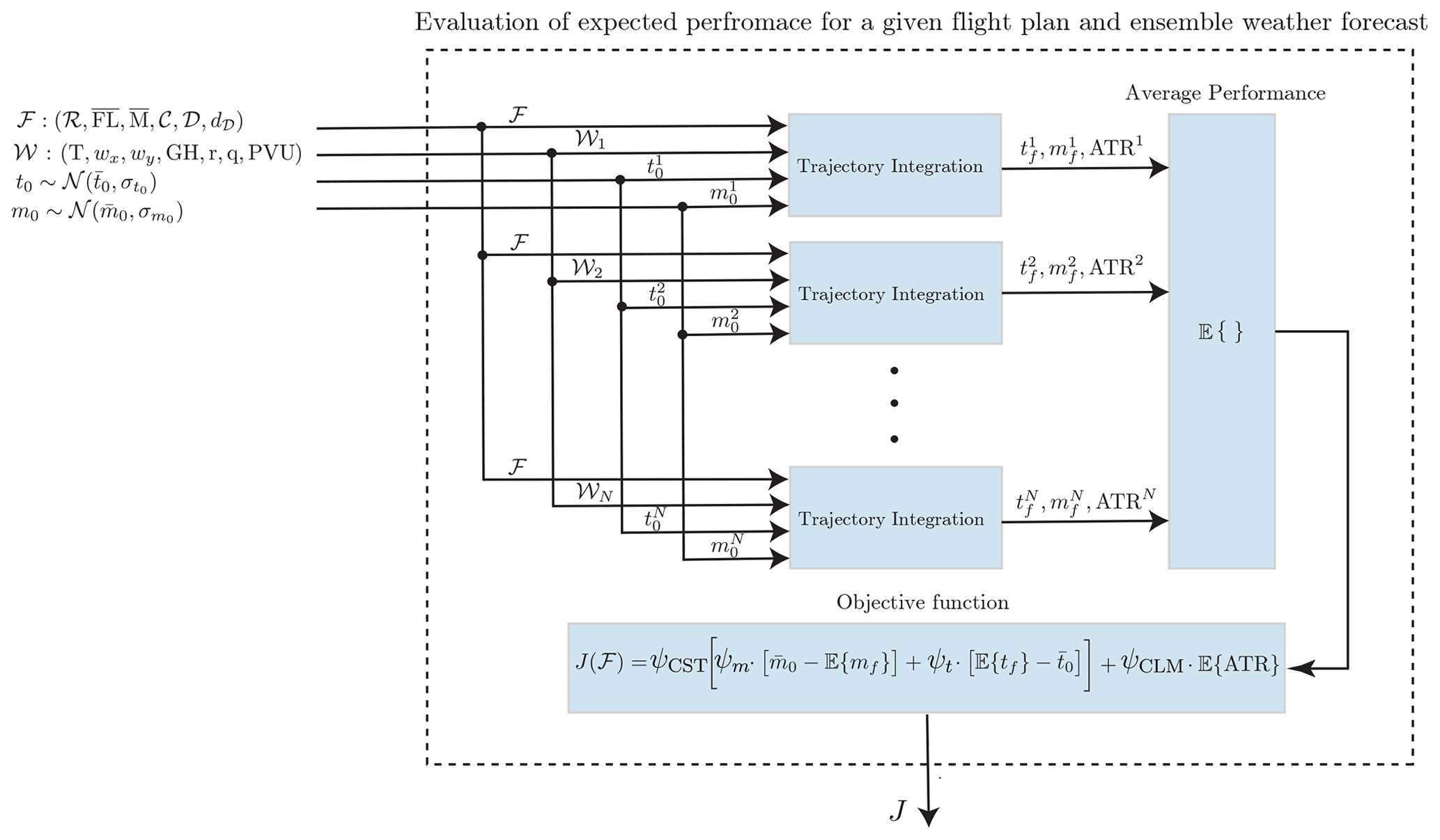
Figure 7Calculation and evaluation of the expected performance for a given flight plan and an ensemble weather forecast.
The objective is to find a flight plan that minimizes Eq. (13). Since the flight plan includes both discrete and continuous decision variables, the optimizer should be capable of solving the optimization within hybrid decision spaces. A classical approach to solving such optimization problems is mixed-integer nonlinear programming, which is mathematically complex and computationally intensive.
3.3 Probabilistic flight plan generation
To solve the optimization with hybrid decision variables in an efficient manner, instead of directly searching for the optimal flight plan, the optimization is conducted in the space of probability distributions defined over flight plans. In other words, instead of directly minimizing minℱJ(ℱ), the minimization of the following equivalent problem is considered:
which provides the same optimal solution; i.e., if ℱ* is the optimal solution to the original problem, provides the same results. The optimization is carried out in the space of probability distributions to move to continuous search space. In addition, it can facilitate searching by parameterizing the distribution p with a parameter vector θ∈ℝΘ, approximating Eq. (14) as
which is generally not identical to Eq. (14), as it relies on whether the parameterization is able to capture a distribution wherein . Thus, the parameterization of the distribution p using the vector θ plays an important role in approximating the original problem. In González-Arribas et al. (2023), the probabilistic-execution flight plan (𝒫ℱ) is introduced to parameterize the distribution over the space of possible flight plans. In this approach, the parameter vector θ is defined as follows:
where is a vector assigning probability to select each airway, and , , , , and d𝒟 are the parameterized Mach schedule, flight level, climb profile, descent profile, and distance to go, respectively. For a parameter vector θ of a 𝒫ℱ, flight plans can be randomly generated. For instance, let us explain how the lateral path is sampled from a given vector of parameters Υ. First, assume that all waypoints of the graph are processed and limited to two outgoing airways. This can be done by considering virtual edges of zero length for waypoints with more than two outgoing airways. The vector composed of a set of junctions is defined as . At kth junction waypoint, the selection of an airway is done through a random process: for kth entry of a given vector Υ (i.e., υk) and kth entry of a vector containing uniform random variables , the airway is selected as
where S(⋅) is a sigmoid function: . Therefore, for a given vector of parameters Υ and a given vector of random variables, a lateral path (restricted to the structure of airspace) can be sampled. The approach to sampling a complete flight plan from p(ℱ;θ), such as sampling Mach schedule and flight level, is presented in González-Arribas et al. (2023) (see Algorithm 1). It is worth mentioning that the operational aspects and feasibility of the aircraft trajectory are considered within the generation of flight plans. For instance, continuous Mach adjustment is avoided, and the frequency of flight level changes is limited.
3.4 Optimization: augmented random search
In the probabilistic-execution flight plan approach, to sample the flight plan from a given θ, vectors containing random variables are required. Thus, the 𝒫ℱ associated with θ is stochastic. To evaluate for a given θ, sampling of multiple flight plans is required. By generating NFP sets of random variables, NFP flight plans (i.e., FPj for ) can be sampled independently for a given θ. To benefit from the provided NEPS probable realizations of meteorological variables and NEPS samples of exogenous sources of uncertainty (i.e., initial flight time and initial flight mass), we sample NEPS (i.e., NFP=NEPS) potential flight plans for a given θ. In other words, each sampled flight plan is evaluated with one realization of meteorological conditions. In this respect, one can rewrite Eqs. (10) and (13) as
The flight planning problem can now be expressed as the following stochastic optimization problem:
where the objective is to find the optimal value of θ (which parameterizes the probability distribution p(ℱ;θ)) such that a population of randomly sampled flight plans minimizes the expected cost in Eq. (18). Sampling NEPS flight plans and using them in a pairwise manner with ensemble members for trajectory integration to evaluate Eq. (17) is computationally more efficient than sampling a different number of flight plans (NFP≠NEPS) and then evaluating each sampled flight plan with all the ensemble members. This is because, in this case, we only integrate the aircraft trajectory NEPS times instead of performing NFP×NEPS trajectory integrations. In spite of reducing the number of computations, it provides similar results. This is due to the fact that, despite sampling multiple flight plans for the evaluation of the objective function in Eq. (17) for a given θ, as the process goes by, all flight plans converge to a unique flight plan. For instance, let us consider the process of sampling the lateral path presented in Sect. 3.3. The choice of each airway relies on two parameters: υ and ξ. For the first iterations of the optimization algorithm, all outgoing airways from waypoints are almost equally probable. However, with more iterations, the decision variable θ is improved, leading to increasing or decreasing the parameter υ. This parameter converges to a large positive or negative value for the last iterations. For instance, in the case of large υ, , implying S(υk)≥ξk for all the sampled flight plans. Thus, in the end, for the optimal value of θ obtained from optimization, we receive a unique flight plan. In this case, for the similar flight plans that are sampled for the last iterations, the expected flight performance variables obtained (from Eq. 17) using NFP×NEPS and NEPS times trajectory integration will be almost the same.
In this work, the V1 version of the augmented random search (ARS) algorithm adopted from Mania et al. (2018) and González-Arribas et al. (2023) is employed. This is a gradient-like algorithm, which starts from an initial point θ0 and then generates n random search directions ω∈ℝΘ. In the next step, it evaluates and , where is a diagonal matrix, adjusting the relative variations that are allowed between decision variables. Then, the decision variables θ are improved along all search directions proportional to . As can be concluded, at each iteration, we generate 2n different vectors of decision variables (i.e., n search directions with θ+Sω and θ−Sω), and for each decision variable, we sample NEPS flight plans. Therefore, we need to perform trajectory evaluation (i.e., TI) 2n×NEPS times for each iteration. As these calculations are similar (or very similar) and independent from each other, the parallelization on GPUs is beneficial, enabling very fast function evaluation. The algorithms, details on the optimization approach, and also parallelization on GPUs are provided in González-Arribas et al. (2023).
The effectiveness of the proposed optimization algorithm to plan robust climate-optimal aircraft trajectories with respect to uncertain meteorological conditions is analyzed for a flight from Frankfurt to Kyiv for two different days and departure times.
-
Scenario 1: 13 June 2018 at 00:00 UTC is a scenario in which the aircraft flies through areas favorable for the formation of persistent contrails.
-
Scenario 2: 10 December 2018 at 12:00 UTC is a scenario with no formation of persistent contrails.
The dominant climate impact of contrails is the main reason for selecting these two scenarios, providing better insight into the mitigation potentials.
For the route graph, the full airspace graph of the considered days is filtered and processed to include all paths from the end of the standard instrument departures of the origin airport to the beginning of the standard instrument arrivals of the destination airport with the maximum length of 104 % of the shortest path length. The considered aircraft is an Airbus model A320-214, with the engine CFM56-5B4/P. Table 2 provides the required parameters to calculate the NOx emission index of the considered aircraft using BFFM2. The initial flight time and initial mass are modeled as Gaussian variables: t0∼𝒩(00:00 UTC, 660) [s] for scenario 1, t0∼𝒩(12:00 UTC, 660) [s] for scenario 2, and m0∼𝒩(61 600, 164) [kg]. The considered standard deviations for initial flight time and initial flight mass are adopted from the studies conducted by Dalmau et al. (2021) and Benjumea (2003), respectively.
As for meteorological input data, due to ease of availability, the ERA5 Reanalysis data products containing 10 ensemble members are adopted for this study. It is worth mentioning that forecast data with more ensemble members can be similarly employed. Simulations are launched on the NVIDIA GeForce RTX 3090 graphics card, providing 10496 CUDA cores at a clock speed of 1.4 to 1.7 GHz.
(DuBois and Paynter, 2006)Table 2The data obtained from the ICAO data bank to calculate the actual emission index of Airbus model A320-214, with the engine CFM56-5B4/P.
The weighting parameters of the objective function given in Eq. (4) are selected as ψCST=α [–] and [USD K−1], where K is a scaling (or conversion) factor determined as
where, for instance, SOCclimate is the SOC calculated when the optimization objective is only the climate impact or ATRcost is the ATR when the objective is only SOC. is a weighting parameter that penalizes cost versus climate impact in which α=0 is the pure cost-optimal and α=1 is the pure climate-optimal routing strategy. In the simulations, we consider five different values for α in order to explore the trade-off between operating cost and climate impact represented by SOC and ATR, respectively.
4.1 Scenario 1: formation of persistent contrails
We consider a scenario in which the aircraft flies through warming contrails for the cost-optimal routing option. Before presenting the results, the performance of the proposed optimizer in terms of convergence and computational time is analyzed. Since the optimization approach is stochastic, different results may be obtained with different executions. To explore the sensitivity of the optimization method, 50 different runs are performed with similar settings for pure cost- (i.e., α=1.0) and pure climate-optimal (i.e., α=0.0) routing options. Then, the objective gap is calculated considering the best performance obtained from different solutions (i.e., the minimum value of J) as the reference. The convergence performances with averaged values as solid lines, and 0, 10, 90, and 100 percentiles are depicted in Fig. 8. For both cases, with around 700 iterations (≈2.8 s) for the cost-optimal trajectory and 900 iterations (≈3.6 s) for the climate-optimal one, the estimated objective gaps are quickly reduced up to 1 % of the values of the objective functions J. As the climate-optimal routing option is associated with the inclusion of aCCFs calculated from meteorological variables, the optimization is much more complex, which can be validated in Fig. 8. With around 4000 iterations (16 s), the objective gap is reduced up to 0.5 % of J. Consequently, with a maximum of 4000 iterations, nearly optimal performance can be obtained with +0.5 % maximum deviation around the best-obtained value (i.e., the most optimal case).
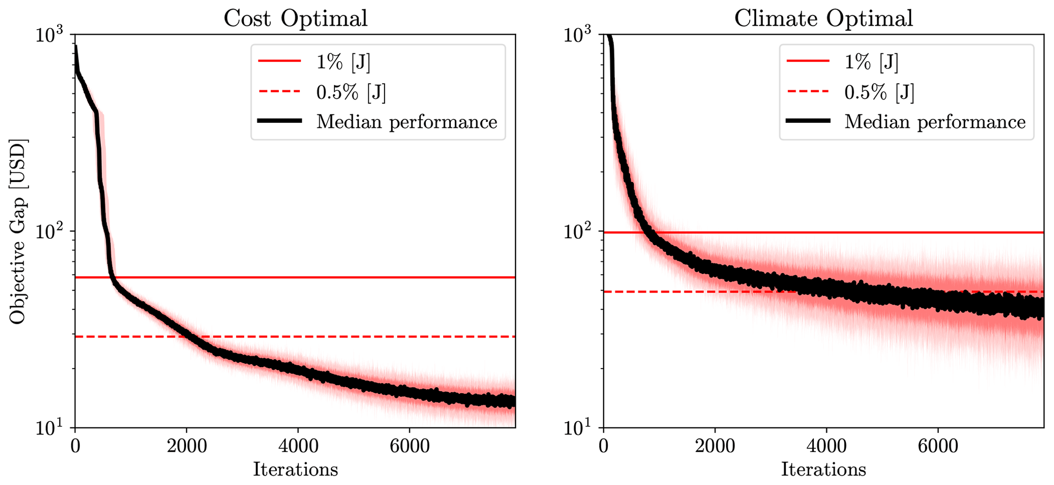
Figure 8Sensitivity of the convergence performance of the optimization algorithm to 50 different executions for the cost- and climate-optimal routing options (α=1 and α=0, respectively) (one iteration ≈4 ms). The objective gap is calculated considering the deviations from the best performance obtained among 50 runs (i.e., the minimum value of J) as the reference, i.e., at each iteration, the value of the objective function (used for trajectory optimization in Eq. 17) is compared with the minimum value obtained from other executions. The mean value is highlighted in as a solid black line, and 0, 10, 90, and 100 percentiles are represented with different color bands.
Now, we proceed to present the obtained results. The aircraft profiles and climate responses for different routing options are given in Fig. 9. The SOC depends on the flight time and fuel consumption. Therefore, the aircraft for routing strategies with higher values of α, such as , tends to fly at higher altitudes within the vertical constraints because flying at higher altitudes is beneficial for reducing fuel consumption, which contributes a large part of the total operating cost (see Fig. 9a). By analyzing the lateral paths depicted in Fig. 10 with the direction and speed of wind at different flight levels, one can see that the aircraft deviates from the shortest path to benefit from stronger tail winds. For trajectories with lower climate impacts, as can be seen in Fig. 9a, the aircraft flies at relatively lower altitudes compared to the cost-optimal routing option, mainly to avoid the formation of persistent contrails (due to warming impacts during nighttime). The climate-optimal routing options reduce the warming effect of contrails. Although the warming climate effects of NOx emissions and water vapor increase with climate-optimal trajectories, the net climate impact decreases. This is because the climate impact of contrails outweighs the impact associated with other species (as discussed in Sect. 2.2.2). The contribution of each species to total climate impact, variability of the obtained climate impacts, and SOC with ranges of uncertainty for different α values and Pareto frontiers are provided in Fig. 11. For a specific case (α=0.2), by accepting an increase of 4.3 % in cost, there is a potential to mitigate the climate impact by 53.0 % considering median performance. In Sect. 2.3, it was shown that the variability of relative humidity among ensemble members is high, leading to high uncertainty in the aCCF of contrails. As expected, the obtained climate impact of contrails is highly uncertain when the aircraft flies through areas sensitive to forming persistent contrails. In contrast, as the aircraft tends to avoid PCFAs, the ranges of uncertainty are reduced, in which, for the complete avoidance that is achieved with α=0.2, the climate impact is almost deterministic. In addition, SOC requires flight time and fuel consumption to represent operating cost in USD, and as it is affected by relatively less uncertain meteorological variables (i.e., wind and temperature compared to relative humidity for the considered case study as analyzed in Sect. 2.3), the uncertainty in its value is small.
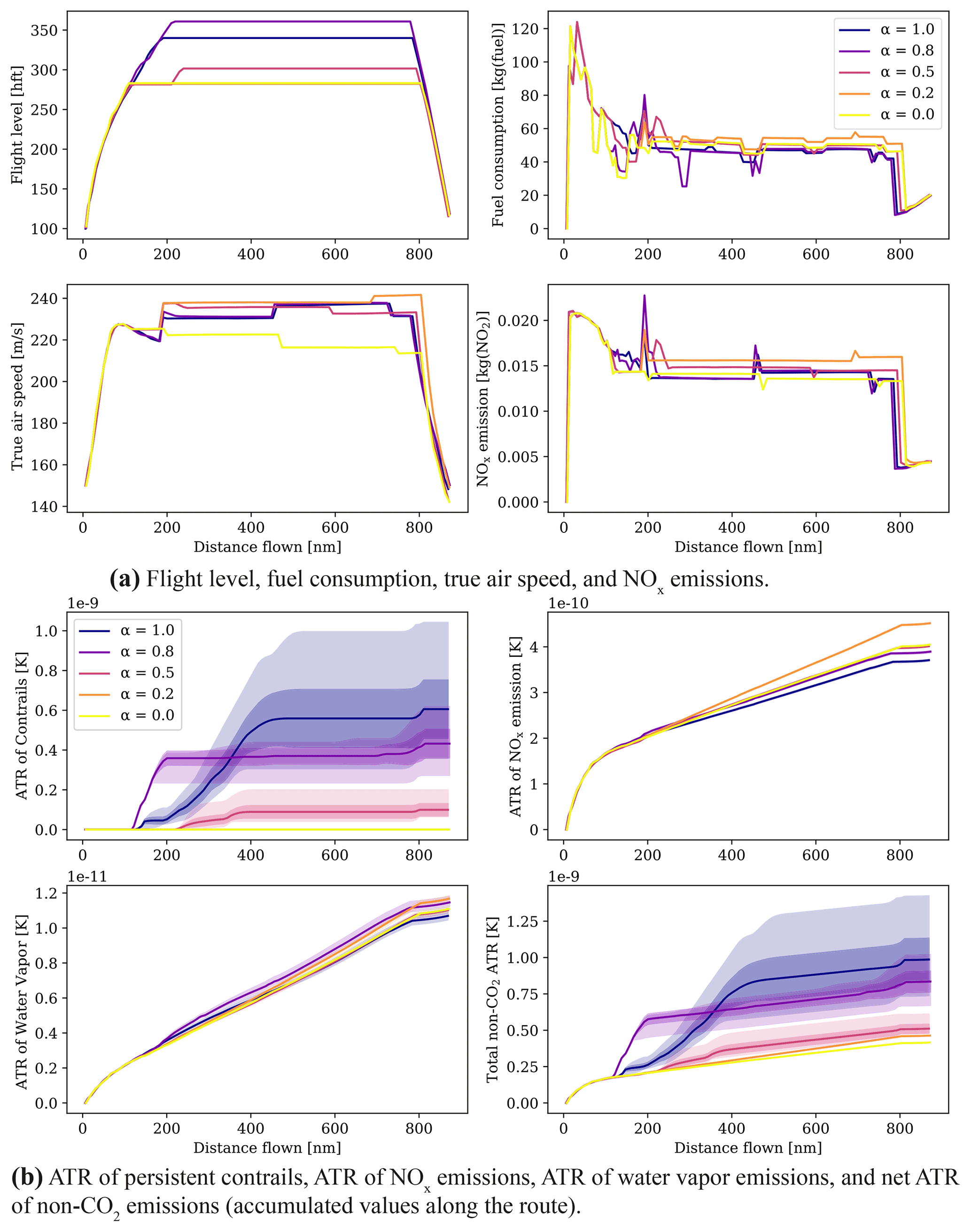
Figure 9Results of scenario 1 (13 June 2018, 00:00 UTC) for different routing options (i.e., α). The shaded regions show the ranges of uncertainty associated with uncertain meteorological conditions (outer lighter areas show the minimum and maximum values, while the inner darker ones represent the 95 % confidence interval).
By analyzing the contribution of each species to the net ATR for different α, one can conclude that the mitigation potential is achieved mainly by avoiding contrail-sensitive areas, which results in slight increases in the climate impact of NOx emissions (see Fig. 11a). However, when the formation of persistent contrails is completely avoided (i.e., with α=0.2), the optimizer tends to reduce NOx emissions mainly by reducing speed to reduce the fuel flow required to calculate the NOx emission index and also total NOx emissions (i.e., NOx emissions = NOx emission index ⋅ fuel consumption). Reducing NOx emissions by flying at lower speeds is achieved at the expense of a considerable increase in flight time and, consequently, SOC. As can be concluded from Pareto frontiers, such a reduction in climate impact for this scenario is not cheap as only 5 % more reduction in climate impact is obtained with almost 3 % more increase in SOC (α=0.0). As the aCCF of contrails is only evaluated in areas favorable for the formation of persistent contrails, typically determined using inequality constraints, it has sharp spatial behaviors (i.e., PCFA (latitude, longitude, altitude, time) ∈ {0, 1}). In addition, contrails have dominant climate effects. Therefore, the optimizer's first choice is to avoid forming persistent contrails, which may be achieved more efficiently than reducing the impacts of other species with relatively lower climate impacts and smooth spatial behaviors. This can be validated in Fig. 11a, as the lowest priority is given to reducing the climate impact associated with NOx emissions (for α=0).
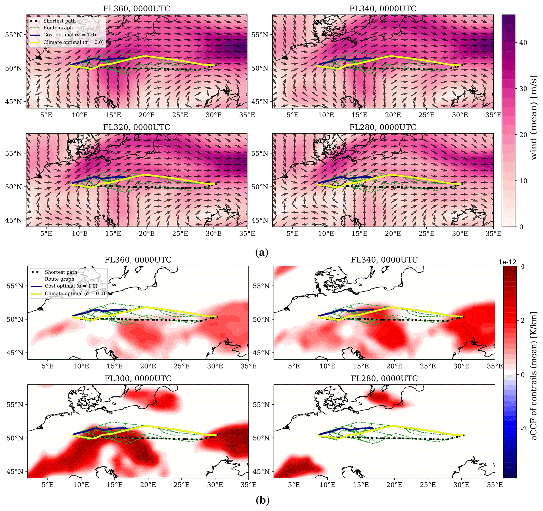
Figure 10Lateral paths for scenario 1 (13 June 2018, 00:00 UTC) depicted with (a) wind and (b) aCCF of contrails as color maps.
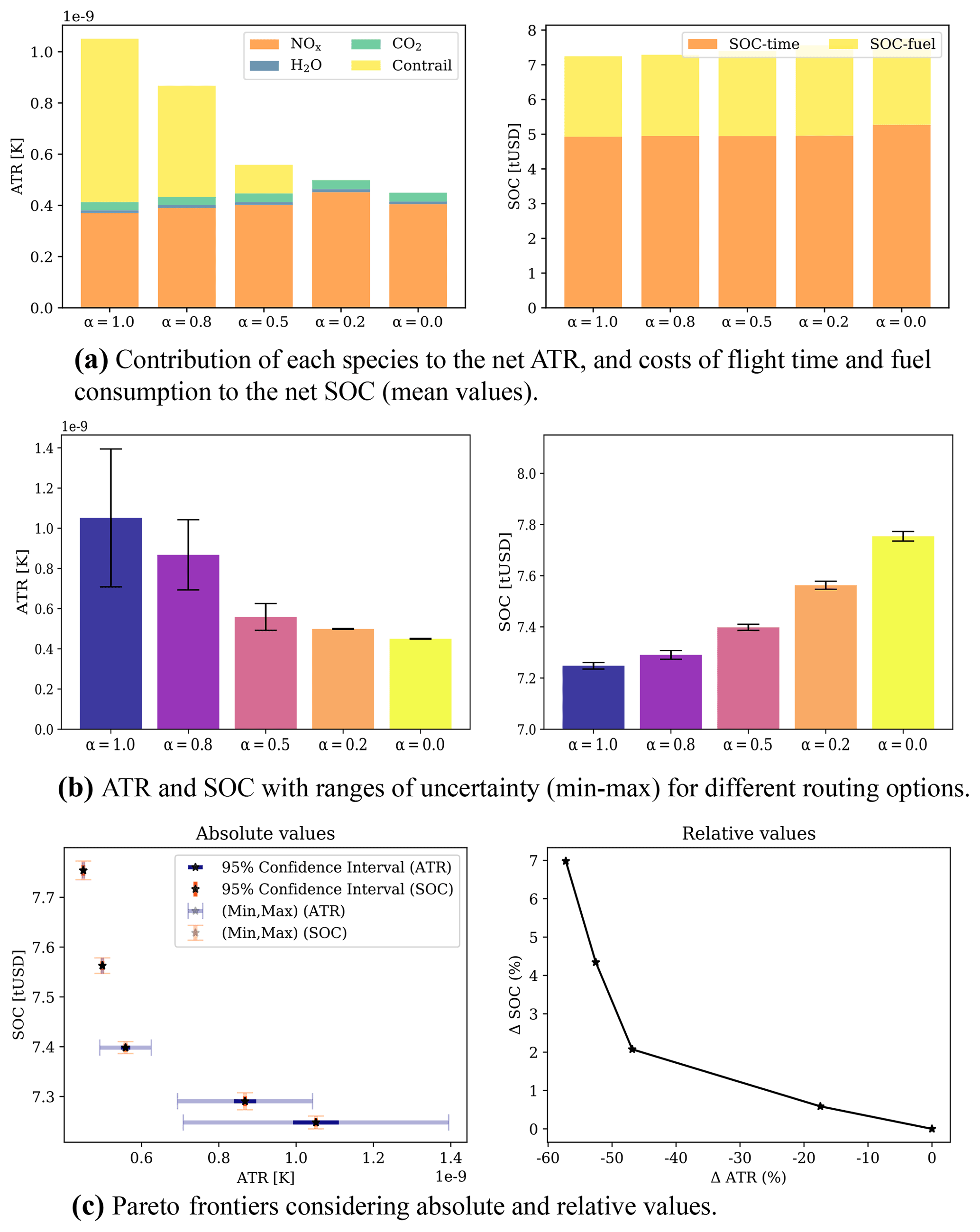
Figure 11Overall performance of the optimized trajectories in terms of ATR and SOC for scenario 1 (13 June 2018, 00:00 UTC).
4.2 Scenario 2: no formation of persistent contrails
In the next scenario, we analyze the mitigation potential when no persistent contrails are formed with the cost-optimal routing option.
For this case, aircraft profiles and climate responses are depicted in Fig. 12a and b, respectively. As can be seen in Fig. 12a, the optimizer chooses to fly at lower altitudes for routing strategies with higher penalization on climate impact. As no persistent contrails are formed (see Fig. 13a), we depict the lateral paths with the merged aCCFs (calculated using the mean values of the obtained NOx emission index) as the color map at different flight levels in Fig. 13b. As can be seen, flying at lower altitudes is more beneficial in reducing the climate impact of other species (mainly NOx). In addition to lowering cruise altitude, the aircraft flies at lower speeds to reduce the fuel flow and, consequently, fuel consumption, NOx emission index, and NOx emissions. The variability of climate impact and SOC for different α values and Pareto frontiers are given in Fig. 14. By reducing α, the climate impact decreases at the cost of an increase in SOC. For instance, for α=0.2, by accepting a 1.1 % increase in cost, a 16 % reduction in ATR can be achieved. As in the previous case, the relative increase in SOC is considerable for α=0, since the aircraft tends to fly at a relatively lower speed for more reduction in climate impact.
In conclusion, climate impact reduction is achieved at the expense of a higher cost increase than in the previous scenario. Moreover, since no contrails are formed, the uncertainty in climate impact is almost negligible.
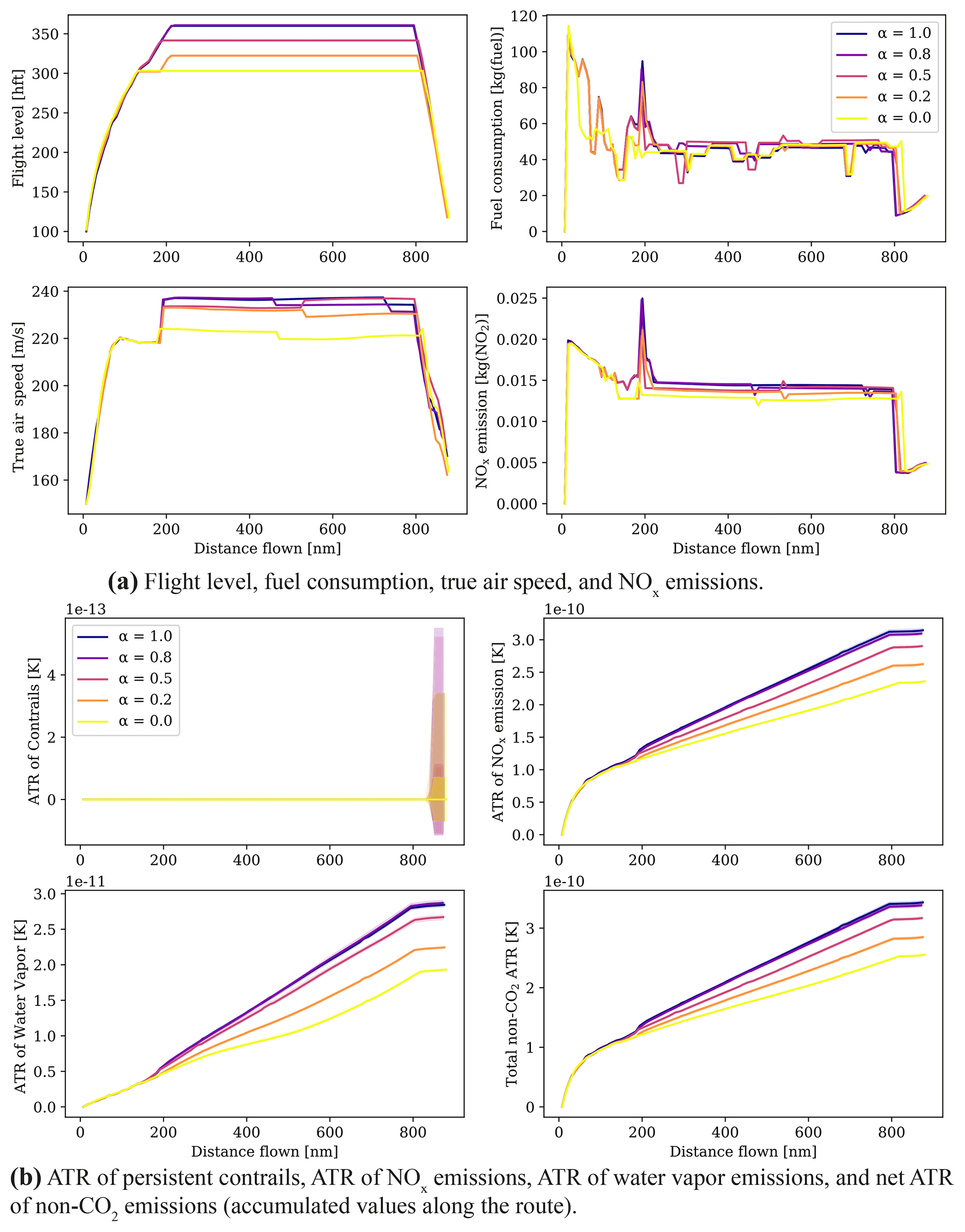
Figure 12Results of scenario 2 (10 December 2018, 12:00 UTC) for different routing options (i.e., α). The shaded regions show the ranges of uncertainty associated with uncertain meteorological conditions (outer lighter areas show the minimum and maximum values, while the inner darker ones represent the 95 % confidence interval).
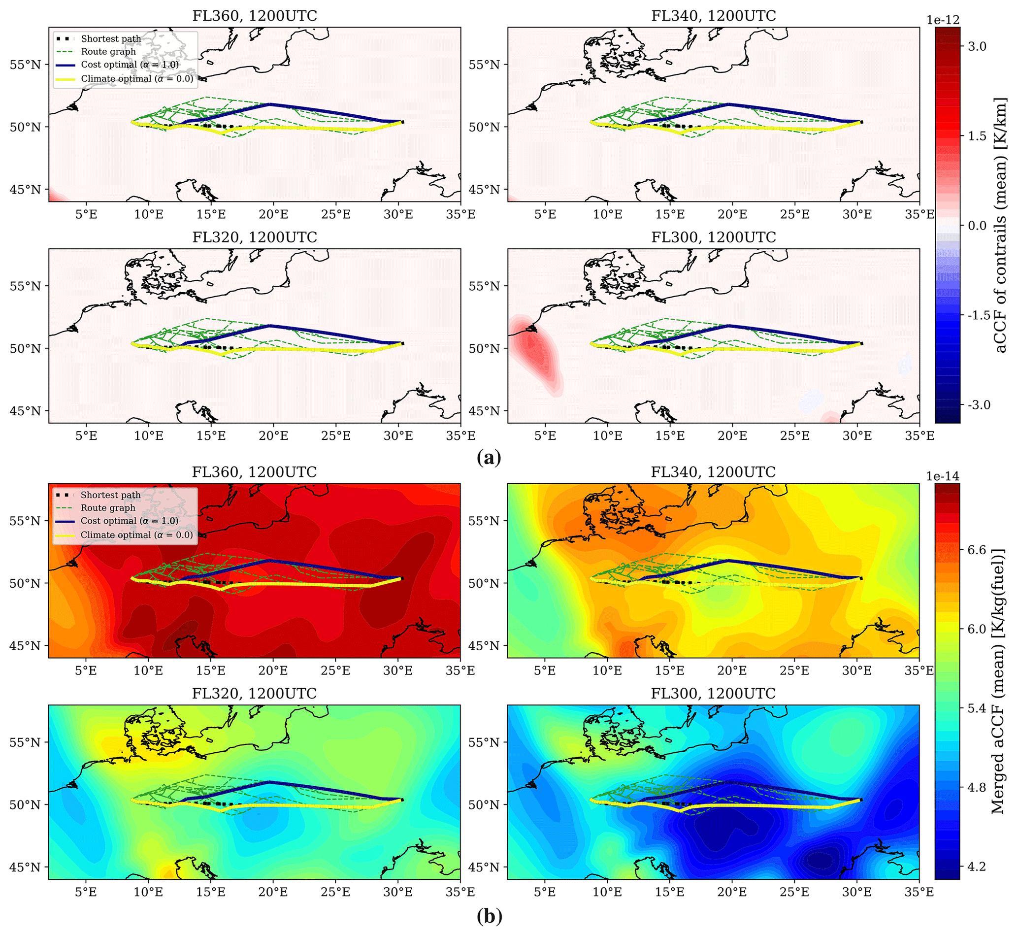
Figure 13Lateral paths with (a) aCCF of contrails and (b) merged aCCFs as color maps at different flight levels for scenario 2 (10 December 2018, 12:00 UTC).
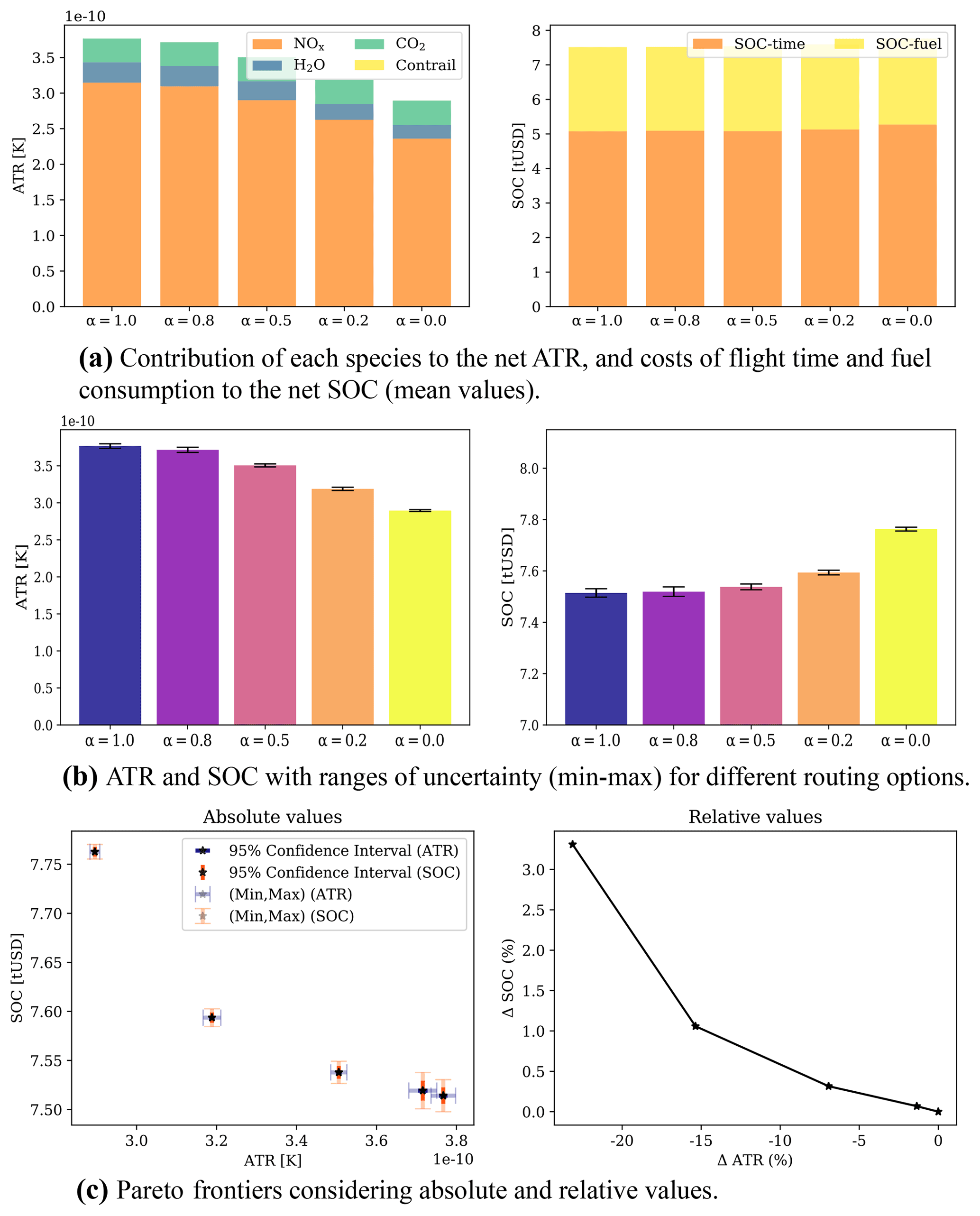
Figure 14Overall performance of the optimized trajectories in terms of ATR and SOC for scenario 2 (10 December 2018, 12:00 UTC).
This paper presented a methodology to plan a robust climate-optimal aircraft trajectory under uncertain meteorological conditions. The climate-sensitive regions were identified using the prototype algorithmic climate change functions (version 1.1). The ensemble prediction system was employed to characterize uncertainty in weather forecasts. A heuristic algorithm was employed and implemented on graphics processing units to solve the proposed robust trajectory optimization in a computationally fast manner. The effectiveness of the proposed approach was explored in two scenarios. Discussion of the obtained results (mainly related to the achieved mitigation potentials, current limitations, and future lines of research) and some general remarks are presented in the following.
The obtained mitigation potentials for the considered scenarios were different due to the variability of meteorological conditions. In both cases, the climate-optimal routing options could reduce the climate impacts. The cost-optimal trajectories flew at higher altitudes compared to climate-optimal ones, as flying at higher altitudes is beneficial for reducing fuel consumption. This is also in line with related studies in the literature (e.g., Yamashita et al., 2020). Due to the dominant climate impact and non-smooth spatial behavior of contrails, the mitigation potential obtained for the scenario with contrail effects (i.e., scenario 1) was higher than the scenario with no formation of persistent contrails. The non-smooth spatial behavior of the contrail climate impact is related to the conditions of PCFA. Due to the high variability among the ensemble members of relative humidity over ice needed to determine PCFA, the climate impact of contrails was highly uncertain. However, for the cases without contrail formation, the total climate impact was almost deterministic. This is because the variability in the other weather variables was almost negligible. For both scenarios, α=0.2 seems to be a reasonable choice, since the climate impacts were reduced at the expense of acceptable increases in the operating cost, and the results were almost deterministic.
In spite of considering the ensemble members in trajectory planning, a unique (or deterministic) flight plan is determined. This reflects the operational feasibility and applicability of this method since, in the flight planning context, the requirement is to determine a unique lateral route in latitude and longitude that starts and ends at predefined points in space and follows the real structure of airspace as well as having a fixed altitude profile and a fixed airspeed schedule. In this case, the effects of uncertainty are reflected in the aircraft performance variables. For instance, let us consider the first scenario. For α=1.0, the lateral path, speed schedule, and flight level were determined in a cost-optimal manner (see Figs. 9a, 10). In our approach, the optimized trajectory is assumed to be tracked as close as possible in practice with the system's low-level controllers in real time. Aiming to optimize a unique flight plan, the proposed method provides some ranges for the aircraft performance variables, such as fuel consumption, flight time, and climate impact, due to different probable realizations of weather conditions. For instance, the climate impact is expected to lie within the determined ranges (see Fig. 9b) if the considered ensemble members could acceptably predict future weather conditions.
One of the next steps should be analyzing the feasibility of such a routing strategy for real traffic scenarios. In fact, air traffic management (ATM) is a complex multi-agent system that cannot be represented by individual elements but by their collective behavior at the network scale. It was shown in the paper that for the climate-optimal routing options, the aircraft tends to fly at relatively lower altitudes compared to the cost-optimal one. Such behavior to avoid climate-sensitive areas may result in more congested areas, raising some challenges, particularly increased workload, complexity, and conflicts. Thus, the mitigation potentials reported at the micro-level may not be achievable considering real traffic scenarios. Therefore, after generating climatically optimal flight plans, one needs to assess the resulting effects at the network scale and perform a resolution (typically modeled as an optimization problem) to re-stabilize the ATM system by compensating for the negative impacts while keeping the modified trajectories as close as possible to inputted climate-optimized ones. The assessment of manageability of climate-optimal trajectory planning in an ATM system is called macro-scale analysis and lies outside the scope of this paper (see Baneshi et al., 2023, for a study in this area).
In this study, we only considered the minimization of the expected performance, e.g., expected climate impact. However, the concept of robustness is mainly related to having less uncertain results (i.e., also minimizing the uncertainty range). In the case of robustness to meteorological uncertainty, we need to find a flight plan that avoids areas of airspace with high variability among the ensemble members. For instance, in González-Arribas et al. (2018), the dispersion of the arrival time is minimized by avoiding regions with high variability among the ensemble members of wind (characterized by SD). In this study, we observed that the most uncertain variable is the climate impact of contrails. Since, for both scenarios, only warming contrails were formed, minimization of the expected values directly led to avoiding uncertain PCFAs, and as can be seen from the results, for the climate-optimized trajectories, we obtained robust solutions (almost deterministic results). However, during the daytime, different behavior is expected for the cases with the cooling contrails. This is because, to reduce the expected climate impact, aircraft will tend to fly in uncertain PCFAs to benefit from cooling effects. In the next versions of ROOST, such scenarios will be taken into account, and controlling the dispersion of all flight performance variables will be addressed by including their variance in addition to the averaged values as objectives in the objective function.
Regarding the computational time and convergence performance, it was shown that they are scenario-dependent. For more complex problems, such as the case including climate impacts quantified by using aCCFs, the optimizer required more iterations to enhance the convergence compared to the cost-optimal routing option. It is worth mentioning that the distance between the origin and destination, available route graphs, and also parameters within the optimization algorithm can change the convergence performance and computational time. The number of iterations is a user-defined parameter that needs to be specified based on the required performance and availability of computational resources. In the performed simulations, we considered 4000 iterations. By looking at the Pareto frontiers, it is clear that the optimizer was able to find nearly optimal solutions. Thanks to the parallelization on GPUs, the computational time for achieving a nearly optimal solution is promising. There are several controlling parameters within the optimization algorithm of ROOST, including the number of search directions, the augmented random search (ARS) step size, and the Nesterov velocity factor (see González-Arribas et al., 2023, for a description of these controlling parameters) that can affect the convergence performance. In our future work, we aim to examine the effects of all these parameters and propose an optimal selection of them. Moreover, adaptive (scenario-dependent) stopping criteria will be proposed, helping to optimize aircraft trajectories more efficiently in the sense of computational time.
To explore the trade-off between climate impact and the operating cost, Pareto frontiers were generated. By changing the weighting parameter α, different Pareto-optimal solutions were obtained. However, with this approach, a specific value for α does not necessarily result in a similar cost increase and climate impact mitigation potential for different scenarios (e.g., for α=0.2, the climate impact is reduced by 53 % and 16 % by accepting a 4.3 % and 1.1 % increase in the operating cost for scenarios 1 and 2, respectively). This approach is suitable for analyzing the mitigation potential for a single flight. However, it is not the most efficient way to study the Pareto-optimal solutions of the aggregated results of a large number of flights. For such cases, having the flexibility to directly optimize flights, requesting a certain range reduction in climate impact or allowing a specific range for the increased operating costs would be beneficial. In this respect, one can aggregate climate-optimal trajectories having, for instance, a 0.5 % to 1.0 % increase in the operating cost. In future versions of ROOST, we will add this feature to the optimization tool by defining some path constraints. Such an aggregation of results is doable with α; however, one needs to generate more points in the Pareto frontier in order to classify the results based on a certain percentage increase in cost or a percentage decrease in climate impact. Scaling up this trajectory-level analysis to the network scale will increase the computational time by a factor of the considered α values.
As was explored in the paper, the mitigation of climate impact within the flight planning context is achieved only by accepting some extra costs due to avoidance of highly climate-sensitive regions, which is in line with related studies in the literature (e.g., Yamashita et al., 2020, 2021; Lührs et al., 2021; Niklaß et al., 2019). One potential approach to offsetting these additional costs is implementing fees and taxes that account for the climate impact caused by aviation in order to motivate airliners to adopt climate-optimal trajectories. Currently, there is no climate policy for the aviation-induced non-CO2 climate effects in the planned market-based instruments such as the emission trading scheme (ETS). However, several studies have proposed frameworks to include costs of aviation-induced non-CO2 climate effects in the operating cost, such as the concept of equivalent CO2 emissions and the concept of climate-charged airspace (Niklaß et al., 2021). If taxes are applied to the non-CO2 climate effects, climate-optimal trajectories can also be economically beneficial.
The aCCFs used in this study represent a prototype formulation. The aCCF algorithms were developed for meteorological summer and winter conditions with a focus on the North Atlantic flight corridor. Thus, the usage of the aCCFs for different seasons and regions needs special caution. However, further development of the aCCFs and an expansion of their geographic scope and seasonal representation represent ongoing research.
The robust aircraft trajectory optimization technique presented in the paper is released as an open-source Python library called ROOST V1.0 (Robust Optimization of Structured Trajectories). It is developed at https://github.com/Aircraft-Operations-Lab/roost (last access: 2 July 2023) and is available via the DOI https://doi.org/10.5281/zenodo.7121862 (Simorgh, 2022). It is distributed under the GNU Lesser General Public License (Version 3.0). All the results presented in the paper were obtained using ROOST. It should be noted that the optimizer ROOST uses BADA4.2 (license granted for the activities developed within the FlyATM4E project) to represent the aerodynamic and propulsive performance of the aircraft. Due to restrictions imposed by the BADA license, the current version (in the GitHub repository) is incomplete, as three Python scripts related to the aircraft performance model used have been excluded (i.e., bada4.py, apm.py, and badalib.cu). We are currently assessing the existing open-source aircraft performance models in order to make the complete library available to the public. In principle, it is possible to use other performance models as long as the functional specification (not necessarily the internal implementation) is the same as the BADA point-mass model, i.e., the drag polar is a function of the same variables, and so on. Otherwise, small modifications to the code would probably have to be applied. Potential alternatives include the OpenAP model (Sun et al., 2020) and the model proposed by Poll and Schumann (2021).
The ERA5 datasets used in this study can be freely accessed from the respective repositories after registration. ERA5 data were retrieved from the Copernicus Climate Data Store (https://doi.org/10.24381/cds.adbb2d47, Hersbach et al., 2023, 2020).
Conceptualization, AS and MS; development of the library (ROOST V1.0), DGA; incorporation of climate impacts to the library, AS; algorithmic climate change functions, SD, SM, and FY; writing – original draft, AS and MS; writing – review and editing, AS, MS, DGA, SM, VG, SD, SB, HY, FL, BL, MMM, FY, and FC. All authors have read and agreed to the published version of the paper.
At least one of the (co-)authors is a member of the editorial board of Geoscientific Model Development. The peer-review process was guided by an independent editor, and the authors also have no other competing interests to declare.
Publisher's note: Copernicus Publications remains neutral with regard to jurisdictional claims in published maps and institutional affiliations.
This research was carried out as a part of the EU project FlyATM4E.
FlyATM4E has received funding from the SESAR Joint Undertaking under the European Union's Horizon 2020 research and innovation program (grant no. 891317). The JU receives support from the European Union's Horizon 2020 research and innovation program and the SESAR JU members other than the union.
This paper was edited by Andrea Stenke and reviewed by two anonymous referees.
AMS-Council: Enhancing weather information with probability forecasts, B. Am. Meteorol. Soc., 89, 1049–1053, 2008. a
Appleman, H.: The formation of exhaust condensation trails by jet aircraft, B. Am. Meteorol. Soc., 34, 14–20, 1953. a
Baneshi, F., Soler, M., and Simorgh, A.: Conflict assessment and resolution of climate-optimal aircraft trajectories at network scale, Transport. Res. D-Tr. E., 115, 103592, https://doi.org/10.1016/j.trd.2022.103592, 2023. a
Bauer, P., Thorpe, A., and Brunet, G.: The quiet revolution of numerical weather prediction, Nature, 525, 47–55, https://doi.org/10.1038/nature14956, 2015. a, b, c
Benjumea, A. C.: Aspectos antropométricos de la población laboral española aplicados al diseño industrial, Instituto Nacional de Seguridad e Higiene en el Trabajo, Ministerio de Trabajo e inmigración, ISBN 84-7425-655-0, 2003 (in Spanish). a
Bickel, M., Ponater, M., Bock, L., Burkhardt, U., and Reineke, S.: Estimating the effective radiative forcing of contrail cirrus, J. Climate, 33, 1991–2005, 2020. a
Bonami, P., Olivares, A., Soler, M., and Staffetti, E.: Multiphase mixed-integer optimal control approach to aircraft trajectory optimization, J. Guid. Control, 36, 1267–1277, 2013. a
Campbell, S., Neogi, N., and Bragg, M.: An optimal strategy for persistent contrail avoidance, in: AIAA Guidance, Navigation and Control Conference and Exhibit, 18–21 August 2008, Honolulu, Hawaii, 6515, 2008. a, b
Dahlmann, K., Grewe, V., Frömming, C., and Burkhardt, U.: Can we reliably assess climate mitigation options for air traffic scenarios despite large uncertainties in atmospheric processes?, Transport. Res. D-Tr. E., 46, 40–55, 2016. a, b
Dalmau, R., Ballerini, F., Naessens, H., Belkoura, S., and Wangnick, S.: An explainable machine learning approach to improve take-off time predictions, J. Air Transp. Manag., 95, 102090, https://doi.org/10.1016/j.jairtraman.2021.102090, 2021. a
Dietmüller, S., Matthes, S., Dahlmann, K., Yamashita, H., Simorgh, A., Soler, M., Linke, F., Lührs, B., Meuser, M. M., Weder, C., Grewe, V., Yin, F., and Castino, F.: A python library for computing individual and merged non-CO2 algorithmic climate change functions: CLIMaCCF V1.0, Geosci. Model Dev. Discuss. [preprint], https://doi.org/10.5194/gmd-2022-203, in review, 2022. a, b, c, d, e, f
DuBois, D. and Paynter, G. C.: “Fuel Flow Method2” for Estimating Aircraft Emissions, SAE Transactions, 1–14, 2006. a, b
Franco Espín, A., Rivas Rivas, D., and Valenzuela Romero, A.: Optimal Aircraft Path Planning in a Structured Airspace Using Ensemble Weather Forecasts, 8th SESAR Innovation Days, 3–7 December 2018, Code 157125, 2018. a
Frömming, C., Grewe, V., Jöckel, P., Brinkop, S., Dietmüller, S., Garny, H., Ponater, M., Tsati, E., and Matthes, S.: Climate cost functions as a basis for climate optimized flight trajectories, Air Traffic Semin., 239, 1–9, 2013. a
Gallo, E., Navarro, F., Nuic, A., and Iagaru, M.: Advanced Aircraft Performance Modeling for ATM: Bada 4.0 Results, in: 2006 ieee/aiaa 25TH Digital Avionics Systems Conference, IEEE, 1–12, https://doi.org/10.1109/dasc.2006.313660, 2006. a
Gierens, K. M., Lim, L., and Eleftheratos, K.: A review of various strategies for contrail avoidance, Open Atmospheric Science Journal, 2, 1–7, 2008. a
González-Arribas, D., Soler, M., and Sanjurjo-Rivo, M.: Robust aircraft trajectory planning under wind uncertainty using optimal control, J. Guid. Control, 41, 673–688, 2018. a, b
González-Arribas, D., Baneshi, F., Andrés, E., Soler, M., Jardines, A., and García-Heras, J.: Fast 4D flight planning under uncertainty through parallel stochastic path simulation, Transport. Res. C-Emer., 148, 104018, https://doi.org/10.1016/j.trc.2023.104018, 2023. a, b, c, d, e, f, g, h, i, j
Graver, B. and Rutherford, D.: Transatlantic airline fuel efficiency ranking, 2017, International Council on Clean Transportation, report, http://www.theicct.org (last access: 2 July 2023), 2018. a
Grewe, V. and Dahlmann, K.: How ambiguous are climate metrics? And are we prepared to assess and compare the climate impact of new air traffic technologies?, Atmos. Environ., 106, 373–374, 2015. a
Grewe, V., Champougny, T., Matthes, S., Frömming, C., Brinkop, S., Søvde, O. A., Irvine, E. A., and Halscheidt, L.: Reduction of the air traffic's contribution to climate change: A REACT4C case study, Atmos. Environ., 94, 616–625, 2014a. a
Grewe, V., Frömming, C., Matthes, S., Brinkop, S., Ponater, M., Dietmüller, S., Jöckel, P., Garny, H., Tsati, E., Dahlmann, K., Søvde, O. A., Fuglestvedt, J., Berntsen, T. K., Shine, K. P., Irvine, E. A., Champougny, T., and Hullah, P.: Aircraft routing with minimal climate impact: the REACT4C climate cost function modelling approach (V1.0), Geosci. Model Dev., 7, 175–201, https://doi.org/10.5194/gmd-7-175-2014, 2014.b. a, b
Guide, D.: CUDA C programming guide, NVIDIA, July, 29, 31, https://docs.nvidia.com/cuda/cuda-c-programming-guide/ (last access: 2 July 2023), 2013. a
Hansen, J., Sato, M., Ruedy, R., Nazarenko, L., Lacis, A., Schmidt, G. A., Russell, G., Aleinov, I., Bauer, M., Bauer, S., Bell, N., Cairns, B., Canuto, V., Chandler, M., Cheng, Y., Del Genio, A., Faluvegi, G., Fleming, E., Friend, A., Hall, T., Jackman, C., Kelley, M., Kiang, N., Koch, D., Lean, J., Lerner, J., Lo, K., Menon, S., Miller, R., Minnis, P., Novakov, T., Oinas, V., Perlwitz, Ja., Perlwitz, Ju., Rind, D., Romanou, A., Shindell, D., Stone, P., Sun, S., Tausnev, N., Thresher, D., Wielicki, B., Wong, T., Yao, M., and Zhang, S.: Efficacy of climate forcings, J. Geophys. Res.-Atmos., 110, https://doi.org/10.1029/2005JD005776, 2005. a
Hartjes, S., Hendriks, T., and Visser, D.: Contrail mitigation through 3D aircraft trajectory optimization, in: 16th AIAA Aviation Technology, Integration, and Operations Conference, 13–17 June 2016, Washington, D.C., USA, 3908, 2016. a, b
Hersbach, H., Bell, B., Berrisford, P., Hirahara, S., Horányi, A., Muñoz-Sabater, J., Nicolas, J., Peubey, C., Radu, R., Schepers, D., Simmons, A., Soci, C., Abdalla, S., Abellan, X., Balsamo, G., Bechtold, P.,Biavati, G., Bidlot, J., Bonavita, M., De Chiara, G., Dahlgren, P., Dee, D., Diamantakis, M., Dragani, R., Flemming, J., Forbes, R., Fuentes, M.,Geer, A., Haimberger, L., Healy, S., Hogan, R. J., Hólm, E., Janisková, M., Keeley, S., Laloyaux, P., Lopez, P., Lupu, C., Radnoti, G., de Rosnay, P., Rozum, I., Vamborg, F., Villaume, S., and Thépaut, J.-N.: The ERA5 global reanalysis, Q. J. Roy. Meteor. Soc., 146, 1999–2049, https://doi.org/10.1002/qj.3803, 2020. a
Hersbach, H., Bell, B., Berrisford, P., Biavati, G., Horányi, A., Muñoz Sabater, J., Nicolas, J., Peubey, C., Radu, R., Rozum, I., Schepers, D., Simmons, A., Soci, C., Dee, D., and Thépaut, J.-N.: ERA5 hourly data on single levels from 1940 to present, Copernicus Climate Change Service (C3S) Climate Data Store (CDS) [data set], https://doi.org/10.24381/cds.adbb2d47 (last access: May 2022), 2023. a
Jelinek, F.: The Advanced Emission Model (AEM3)-Validation Report, Ratio, 306, 1–13, 2004. a
Klöckner, A., Pinto, N., Lee, Y., Catanzaro, B., Ivanov, P., and Fasih, A.: PyCUDA and PyOpenCL: A scripting-based approach to GPU run-time code generation, Parallel Comput., 38, 157–174, 2012. a
Lee, D. S., Fahey, D. W., Skowron, A., Allen, M. R., Burkhardt, U., Chen, Q., Doherty, S. J., Freeman, S., Forster, P. M., Fuglestvedt, J., Gettelman, A., De Leon, R. R., Lim, L. L., Lund, M. T., Millar, R. J., Owen, B., Penner, J. E., Pitari, G., Prather, M. J., Sausen, R., and Wilcox, L. J.: The contribution of global aviation to anthropogenic climate forcing for 2000 to 2018, Atmos. Environ., 244, 117834, https://doi.org/10.1016/j.atmosenv.2020.117834, 2021. a, b, c, d
Lim, Y., Gardi, A., and Sabatini, R.: Optimal aircraft trajectories to minimize the radiative impact of contrails and CO2, Energy Proced., 110, 446–452, 2017. a
Lührs, B., Niklass, M., Froemming, C., Grewe, V., and Gollnick, V.: Cost-benefit assessment of 2D and 3D climate and weather optimized trajectories, in: 16th AIAA Aviation Technology, Integration, and Operations Conference, 13–17 June 2016, Washington, D.C., USA, 3758, 2016. a, b
Lührs, B., Linke, F., Matthes, S., Grewe, V., and Yin, F.: Climate impact mitigation potential of European air traffic in a weather situation with strong contrail formation, Aerospace, 8, 50, https://doi.org/10.3390/aerospace8020050, 2021. a, b, c, d, e
Mania, H., Guy, A., and Recht, B.: Simple random search of static linear policies is competitive for reinforcement learning, in: Advances in Neural Information Processing Systems, edited by: Bengio, S., Wallach, H., Larochelle, H., Grauman, K., Cesa-Bianchi, N., and Garnett, R., Neural Information Processing Systems Foundation, Inc. (NeurIPS), ISBN 9781510884472, 1800–1809, 2018. a
Matthes, S., Schumann, U., Grewe, V., Frömming, C., Dahlmann, K., Koch, A., and Mannstein, H.: Climate optimized air transport, in: Atmospheric physics, edited by: Schumann, U., Springer, 727–746, https://doi.org/10.1007/978-3-642-30183-4_44, 2012. a
Matthes, S., Grewe, V., Dahlmann, K., Frömming, C., Irvine, E., Lim, L., Linke, F., Lührs, B., Owen, B., Shine, K., Stromatas, S., Yamashita, H., and Yin, F.: A concept for multi-criteria environmental assessment of aircraft trajectories, Aerospace, 4, 42, https://doi.org/10.3390/aerospace4030042, 2017. a, b
Matthes, S., Lührs, B., Dahlmann, K., Grewe, V., Linke, F., Yin, F., Klingaman, E., and Shine, K. P.: Climate-optimized trajectories and robust mitigation potential: Flying ATM4E, Aerospace, 7, 156, https://doi.org/10.3390/aerospace7110156, 2020. a, b
Matthes, S., Dietmüller, S., Dahlmann, K., Frömming, C., Yamashita, H., Grewe, V., Yin, F., and Castino, F.: Algorithmic climate change functions (aCCFs) V1.0A: Consolidation of the approach and note for usage, Geosci. Model Dev. Discuss., submitted, 2023. a, b, c
Niklaß, M., Gollnick, V., Lührs, B., Dahlmann, K., Froemming, C., Grewe, V., and van Manen, J.: Cost-benefit assessment of climate-restricted airspaces as an interim climate mitigation option, J. Air Transport., 25, 27–38, 2017. a, b
Niklaß, M., Lührs, B., Grewe, V., Dahlmann, K., Luchkova, T., Linke, F., and Gollnick, V.: Potential to reduce the climate impact of aviation by climate restricted airspaces, Transport Policy, 83, 102–110, 2019. a, b
Niklaß, M., Grewe, V., Gollnick, V., and Dahlmann, K.: Concept of climate-charged airspaces: a potential policy instrument for internalizing aviation's climate impact of non-CO2 effects, Climate Policy, 21, 1066–1085, 2021. a, b
Penner, J. E., Lister, D., Griggs, D. J., Dokken, D. J., and McFarland, M.: Aviation and the global atmosphere: a special report of the Intergovernmental Panel on Climate Change, ISBN-10 0521663008, ISBN-13 978-0521663007, 1999. a
Poll, D. and Schumann, U.: An estimation method for the fuel burn and other performance characteristics of civil transport aircraft in the cruise. Part 1 fundamental quantities and governing relations for a general atmosphere, Aeronaut. J., 125, 257–295, 2021. a
Ponater, M., Grewe, V., Sausen, R., Schumann, U., Pechtl, S., Highwood, E., and Stuber, N.: Climate sensitivity of radiative impacts from transport systems, in: Proceedings of an International Conference on Transport, Atmosphere and Climate (TAC), Proceedings of the TAC-Conference, 26 to 29 June 2006, Oxford, UK, 190–196, 2007. a, b
Rap, A., Forster, P. M., Haywood, J. M., Jones, A., and Boucher, O.: Estimating the climate impact of linear contrails using the UK Met Office climate model, Geophys. Res. Lett., 37, L20703, https://doi.org/10.1029/2010GL045161, 2010. a
Scherer, C.: Global Market Forecast Cities, Airports & Aircraft 2019-2038, AIRBUS SAS, 31707, ISBN 978-2-9554382-4-6, 2019. a
Schmidt, E.: Die entstehung von eisnebel aus den auspuffgasen von flugmotoren, Schriften der Deutschen Akademie der Luftfahrtforschung, Verlag R. Oldenbourg, München, Heft 44, 5, 1–15, 1941. a
Simorgh, A.: Abolfazl-Simorgh/roost: Initial Release (v0.1.0), Zenodo [code], https://doi.org/10.5281/zenodo.7121862, 2022. a, b
Simorgh, A., Soler, M., González-Arribas, D., Matthes, S., Grewe, V., Dietmüller, S., Baumann, S., Yamashita, H., Yin, F., Castino, F., Linke, F., Lührs, B., and Meuser, M. M.: A Comprehensive Survey on Climate Optimal Aircraft Trajectory Planning, Aerospace, 9, 146, https://doi.org/10.3390/aerospace9030146, 2022. a, b, c, d, e, f, g, h, i
Soler, M., Zou, B., and Hansen, M.: Flight trajectory design in the presence of contrails: Application of a multiphase mixed-integer optimal control approach, Transport. Res. C-Emer., 48, 172–194, 2014. a
Sridhar, B., Ng, H. K., and Chen, N. Y.: Aircraft trajectory optimization and contrails avoidance in the presence of winds, J. Guid. Control, 34, 1577–1584, 2011. a, b
Sun, J., Hoekstra, J. M., and Ellerbroek, J.: OpenAP: An open-source aircraft performance model for air transportation studies and simulations, Aerospace, 7, 104, https://doi.org/10.3390/aerospace7080104, 2020. a
van Manen, J. and Grewe, V.: Algorithmic climate change functions for the use in eco-efficient flight planning, Transport. Res. D-Tr. E., 67, 388–405, 2019. a
Vitali, A., Battipede, M., and Lerro, A.: Multi-Objective and Multi-Phase 4D Trajectory Optimization for Climate Mitigation-Oriented Flight Planning, Aerospace, 8, 395, https://doi.org/10.3390/aerospace8120395, 2021. a
WMO: Guidelines on ensemble prediction systems and forecasting, edited by: Svoboda, M., Hayes, M., and Wood, D. A., World Meteorological Organization Weather Climate and Water, 1091, ISBN 978-92-63-11091-6, 2012. a
Yamashita, H., Yin, F., Grewe, V., Jöckel, P., Matthes, S., Kern, B., Dahlmann, K., and Frömming, C.: Newly developed aircraft routing options for air traffic simulation in the chemistry–climate model EMAC 2.53: AirTraf 2.0, Geosci. Model Dev., 13, 4869–4890, https://doi.org/10.5194/gmd-13-4869-2020, 2020. a, b, c, d, e, f, g
Yamashita, H., Yin, F., Grewe, V., Jöckel, P., Matthes, S., Kern, B., Dahlmann, K., and Frömming, C.: Analysis of aircraft routing strategies for north atlantic flights by using AirTraf 2.0, Aerospace, 8, 33, https://doi.org/10.3390/aerospace8020033, 2021. a, b, c
Yin, F., Grewe, V., Frömming, C., and Yamashita, H.: Impact on flight trajectory characteristics when avoiding the formation of persistent contrails for transatlantic flights, Transport. Res. D-Tr. E., 65, 466–484, 2018a. a, b
Yin, F., Grewe, V., van Manen, J., Matthes, S., Yamashita, H., Linke, F., and Lührs, B.: Verification of the ozone algorithmic climate change functions for predicting the short-term NOx effects from aviation en-route, in: International Conference on Research in Air Transportation (ICRAT), 26–29 June 2018, Castelldefels, Barcelona, Spain, https://repository.tudelft.nl/islandora/object/uuid:3eab3d00-2728-4220-8d3e-0eef4cae8a11?collection=research (last access: 2 July 2023), 2018b. a
Yin, F., Grewe, V., Castino, F., Rao, P., Matthes, S., Dahlmann, K., Dietmüller, S., Frömming, C., Yamashita, H., Peter, P., Klingaman, E., Shine, K., Lührs, B., and Linke, F.: Predicting the climate impact of aviation for en-route emissions: The algorithmic climate change function submodel ACCF 1.0 of EMAC 2.53, Geosci. Model Dev. Discuss. [preprint], https://doi.org/10.5194/gmd-2022-220, in review, 2022. a, b, c