the Creative Commons Attribution 4.0 License.
the Creative Commons Attribution 4.0 License.
 | 08 Jun 2023
A wind-driven snow redistribution module for Alpine3D v3.3.0: adaptations designed for downscaling ice sheet surface mass balance
Eric Keenan
Jan T. M. Lenaerts
Brooke Medley
Ice sheet surface mass balance describes the net snow accumulation at the ice sheet surface. On the Antarctic ice sheet, winds redistribute snow, resulting in a surface mass balance that is variable in both space and time. Representing wind-driven snow redistribution processes in models is critical for local assessments of surface mass balance, repeat altimetry studies, and interpretation of ice core accumulation records. To this end, we have adapted Alpine3D, an existing distributed snow modeling framework, to downscale Antarctic surface mass balance to horizontal resolutions up to 1 km. In particular, we have introduced a new two-dimensional advection-based wind-driven snow redistribution module that is driven by an offline coupling between WindNinja, a wind downscaling model, and Alpine3D. We then show that large accumulation variability can be at least partially explained by terrain-induced wind speed variations which subsequently redistribute snow around rolling topography. By comparing Alpine3D to airborne-derived snow accumulation measurements within a testing domain over Pine Island Glacier in West Antarctica, we demonstrate that our Alpine3D downscaling approach improves surface mass balance estimates when compared to the Modern-Era Retrospective analysis for Research and Applications, Version 2 (MERRA-2), a global atmospheric reanalysis which we use as atmospheric forcing. In particular, when compared to MERRA-2, Alpine3D reduces simulated surface mass balance root mean squared error by 23.4 (13 %) and increases variance explained by 24 %. Despite these improvements, our results demonstrate that considerable uncertainty stems from the employed saltation model, confounding simulations of surface mass balance variability.
- Article
(9750 KB) - Full-text XML
- BibTeX
- EndNote


Ice sheet surface mass balance (SMB) is the difference between mass accumulation and ablation processes at the surface of ice sheets (Lenaerts et al., 2019). Mass accumulation is composed of precipitation as well as condensation and deposition of atmospheric water vapor, whereas ablation processes remove mass from the ice sheet surface via meltwater runoff, both atmospheric and surface sublimation, and evaporation. Additionally, local SMB is influenced by the process of wind-driven snow redistribution, which we refer to as deposition in the case of local mass gain and erosion in the case of mass loss (Lenaerts and van den Broeke, 2012). Wind-driven snow redistribution is generally divided into two categories, drifting snow, where snow particles are transported by the wind in the lowermost 2 m of the atmosphere, and blowing snow, where snow is redistributed at heights greater than 2 m.
Drifting snow and blowing snow have been shown to have a substantial effect on Antarctic SMB spatial variability at scales ranging from tens of kilometers (Dattler et al., 2019a; Kausch et al., 2020) to meters (Picard et al., 2019). In fact, both Dattler et al. (2019a) and Picard et al. (2019) have shown that local deposition can exceed annual precipitation. In addition to redistributing mass, drifting snow and blowing snow contribute to mass loss by promoting enhanced sublimation as snow particles are entrained in the lower atmosphere (Palm et al., 2017). In spite of drifting and blowing snow sublimation being a source of mass loss, evaluation of model simulation of these processes remains difficult (Amory et al., 2021). The net effect of drifting snow and blowing snow is preferential deposition in areas of mass convergence at the expense of areas with net divergence (Lehning et al., 2008). Despite our lack of complete physical understanding of the processes which govern preferential deposition at small spatial and temporal scales (Comola et al., 2019b), deposition and erosion can be conceptually summarized as the local convergence of previously eroded snow particles from upwind minus locally eroded snow (Liston et al., 2007). Local erosion is governed by the direct competition between forces that act to erode snow and those which act to anchor snow to the ice sheet surface. Erosive forces, i.e., surface wind stress, are controlled by atmospheric boundary layer processes (Paterna et al., 2016; Comola et al., 2019a), while cohesive forces are controlled by snow microstructural properties including grain size and bond strength (Clifton et al., 2006; Melo et al., 2022). This interplay between boundary layer and snow microstructural processes has historically motivated the development of tightly coupled atmospheric and land surface snow models (e.g., Lawrence et al., 2019; Amory et al., 2021; Sharma et al., 2023).
When the combined effect of surface wind stress and impact force from saltating particles exceeds cohesive forces at the snow surface, saltation of snow particles is initiated or maintained within the lowermost 10 cm of the atmosphere (Schmidt, 1980; Pomeroy and Gray, 1990). Within the saltation layer, atmospheric momentum is entrained by snow particles which eventually collide with and subsequently mobilize additional particles at the snow surface. Above the saltation layer, a suspension layer can be present where turbulent eddies generate sufficient upward lift forces that can keep particles afloat against gravity (e.g., Bintanja, 2000). Measurements from Antarctica show that particles in suspension are typically much smaller than those that are transported in saltation (Nishimura and Nemoto, 2005). Correspondingly, mass densities in the suspension layer are found to be orders of magnitude smaller than in the saltation layer. However, with increasing wind speed, the suspension layer can grow orders of magnitude larger than the height of the saltation layer, leading to estimates that the largest part of total mass transport during high-wind-speed events could be carried in the suspension layer (Pomeroy and Male, 1992; Liston and Sturm, 1998; Mann, 1998). It is difficult to quantify the contribution of suspension to total mass transport on average, with some authors arguing that saltation accounts for 50 %–75 % of total wind-driven mass transport (Gromke et al., 2014). However, although deposition and erosion are ubiquitous across much of the Antarctic ice sheet, it is possible that local SMB variability is primarily driven by a small number of high-wind-speed events which occur only a few times per year.
Nevertheless, the interaction between wind transport of snow and the snow surface is governed by the saltation layer. As saltating particles break apart upon collision with the surface, snow grain fragmentation and rounding are observed, resulting in increased density (Vionnet et al., 2012; Amory et al., 2021) in a processes referred to as drifting-snow compaction. Reliable model representation of drifting-snow compaction is now particularly attractive owing to recent advancements in satellite altimetry technology (e.g., CryoSat-2 and ICESat-2). Vertical accuracy, spatial resolution, and ground track repeat frequency have all increased, providing precise measurements of ice sheet surface height change (Smith et al., 2020). However, in order to reliably convert these height changes into mass, particularly over short timescales, we rely on accurate snow and firn density estimates from models (The IMBIE team, 2018). Thus, to confidently assign subtle observed changes in height to quantifiable changes in mass, our models must capture the complex spatial and temporal patterns of deposition and erosion.
Current state-of-the-art firn densification models, which are used to convert satellite-observed volume changes into mass, successfully capture broad regional variability in firn properties, including density (Ligtenberg et al., 2011; Medley et al., 2022b). However, because of the relatively coarse horizontal resolutions at which they are applied (5.5–35 km), these models are unable to represent spatial variability in firn processes, including deposition and erosion, at the horizontal scales now sampled by satellites (<1 km). This spatial gap between satellite observations and firn densification models may not be immediately important for mass balance retrievals at continental scales (Verjans et al., 2021). Nevertheless, improved model representation of wind-driven snow redistribution at finer spatial scales can be used to constrain regional to local surface mass balances (Rignot et al., 2011), improve volume-to-mass conversions for repeat altimetry (Shepherd et al., 2012; Zwally et al., 2015), provide the ice-coring and radar communities with a mechanism to select representative sampling locations for SMB reconstructions (Kausch et al., 2020), and inform future studies by providing baselines to estimate sublimation of drifting and blowing snow.
To facilitate local SMB estimates and reconstructions and to repeat altimetry interpretation, we present a new technique for dynamically downscaling Antarctic SMB by building upon the existing Alpine3D v3.3.0 model framework (Sect. 2.1). Alpine3D already contains a module for the three-dimensional treatment of drifting and blowing snow (Lehning et al., 2006), but its use requires three-dimensional wind fields at high temporal resolution from an external source, and it is computationally very demanding to run. This motivates the current study to find a simpler and therefore computationally lighter method to describe wind transport by snow, particularly since the fully three-dimensional approach also does not guarantee good agreement between simulated and observed snow depth in severely wind-affected areas (Mott et al., 2008, 2010; Gerber et al., 2017). To this end, we describe the use of WindNinja to downscale wind fields onto local topography (Sect. 2.2), demonstrate the use of a one-dimensional snow model to diagnose local erosion (Sect. 2.3) and then distribute this mass horizontally across adjacent grid cells using a new, two-dimensional advection-based redistribution module (Sect. 2.4). We then present downscaling results at 1 and 3 km horizontal resolution and evaluate the added value by quantitatively comparing our results, along with a global SMB product, to a 130 km-long airborne-radar-derived SMB transect in interior West Antarctica over Pine Island Glacier (Sect. 3.1–3.2, 3.5).
2.1 Alpine3D: surface mass balance downscaling framework
We use and further develop the existing Alpine3D v3.3.0 model framework (Lehning et al., 2006) to downscale Antarctic SMB processes to a target horizontal resolution of up to 1 km. At its core, the model framework exploits the MeteoIO library (Bavay and Egger, 2014) to handle meteorological preprocessing and downscaling (Sect. 2.2), SNOWPACK (Bartelt and Lehning, 2002; Lehning et al., 2002b, a), a physics-based land-surface snow model for the detailed description of snow microstructural properties (Sect. 2.3), and a new module to calculate horizontal mass fluxes between adjacent grid cells (Sect. 2.4 and 2.6, Fig. 1).
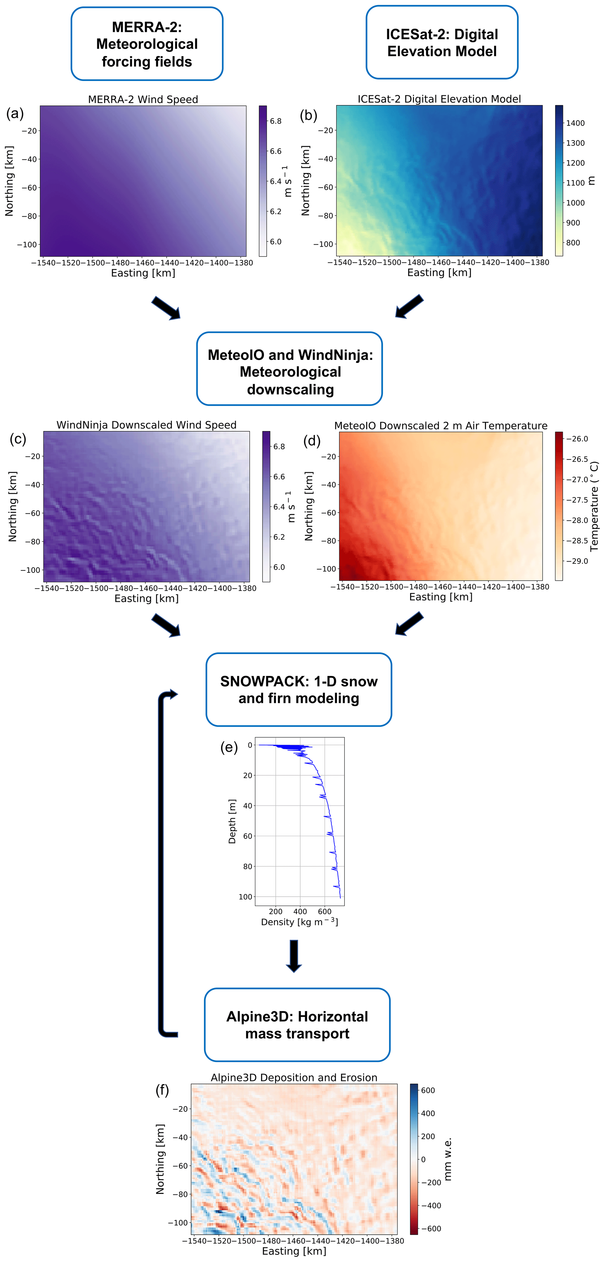
Figure 1Anatomy of an Alpine3D time step: hourly global atmospheric reanalysis (a) is combined with ICESat-2-derived surface topography (b) to calculate downscaled meteorology (c, d) at each SNOWPACK model grid cell. The SNOWPACK model is then used to calculate snow microstructural properties at each grid cell (e). Finally, the Alpine3D model is used to calculate horizontal mass transport across adjacent grid cells (f), which is then sent back to SNOWPACK for the next time step. Note that, in panels (c) and (d), downscaled wind speed and 2 m air temperature are shown as an example, while relative humidity, incoming shortwave and longwave radiation, precipitation rate, and 10 m wind direction are also downscaled (see text).
2.2 Atmospheric forcing: meteorological downscaling
At the snow surface, we prescribe hourly MERRA-2 global atmospheric reanalysis (Gelaro et al., 2017), which we have downscaled to the Alpine3D grid using the MeteoIO preprocessing and downscaling library (Bavay and Egger, 2014). These downscaled time series include 2 m air temperature, relative humidity, incoming shortwave and longwave radiation (ISWR and ILWR), precipitation rate, and 10 m wind speed and direction; 2 m air temperature is first downscaled to the Alpine3D grid using an ordinary kriging algorithm with a lapse rate of −6 designed to capture a typical atmospheric lapse rate (Martin and Peel, 1978), while relative humidity is spatially interpolated according to Liston and Elder (2006). Precipitation rate and ISWR are then interpolated using inverse distance weighting, with ISWR undergoing a simple correction for slope and topographic shading (Helbig, 2009). ILWR is interpolated by first calculating the hourly average of all MERRA-2 grid cells within the domain and then applying a constant lapse rate of −31.25 (Michel et al., 2022). We follow Keenan et al. (2021) by applying the MERRA-2 mean annual surface temperature as a Dirichlet thermodynamic boundary condition at the bottom of the firn column. This assumption is supported by observations from the dry snow zone of the Greenland ice sheet, where differences between mean annual air temperature and firn temperature at 10 m were found to be typically within a few tenths of a degree (Alley and Koci, 1990). Ligtenberg (2014) also shows in a model result that the seasonal cycle in firn temperature disappears around 10 m depth. Note that, for all topographic calculations, we use an ICESat-2-derived digital elevation model (DEM) (Medley et al., 2022a).
Because reliable simulations of deposition and erosion require accurate wind speed and direction fields (Reynolds et al., 2021), we test two approaches for downscaling wind speed and direction from the relatively coarse (0.5∘ latitude × 0.625∘ longitude) MERRA-2 grid. First, we apply the terrain-based index method proposed by Liston et al. (2007), which adjusts wind speed and direction based on topographic exposure and sheltering. Note that we use the default slope and curvature weighting factors and choose a topographic length scale of 5 km. However, because Reynolds et al. (2021) showed that simulated snow depth better captured observations when forced with WindNinja downscaled wind fields (Forthofer et al., 2014) compared to the relatively simpler terrain-based index methods presented in Liston et al. (2007), we have implemented WindNinja (Version 3.7.1) as an alternative offline wind speed and direction downscaling technique within the Alpine3D modeling framework. WindNinja is a finite-element diagnostic model which leverages a mass conservation solver and DEM to simulate the mechanical effects of terrain on the flow. In terms of WindNinja model configuration, we have selected the “fine” finite-element mesh resolution and chosen “grass” as our surface roughness category (snow is not currently an option). Despite representing a significant increase in complexity compared to other terrain-based interpolation techniques (e.g., Liston et al., 2007), WindNinja is still computationally cheaper than high-resolution numerical weather models (e.g., the Weather Research and Forecasting (WRF) model) which solve the non-hydrostatic, fully compressible Navier–Stokes equations at multiple vertical levels (Wagenbrenner et al., 2016) and can therefore be run with reasonable computational resources (Sect. 2.6).
2.3 SNOWPACK: one-dimensional physics-based snow model
We use SNOWPACK, a physics-based land surface snow model, to describe one-dimensional snow and firn processes at each Alpine3D grid cell. SNOWPACK was originally developed for avalanche warning applications and has been continuously enhanced in order to represent various cryospheric processes, including seasonal snow (Sharma et al., 2023), sea ice snow cover (Wever et al., 2020), and polar firn compaction (Groot Zwaaftink et al., 2013; Keenan et al., 2021). In this study, we use the SNOWPACK physics presented in Keenan et al. (2021), with one exception being a new parameterization for surface roughness length, z0 (m, Eq. 1), tuned to observed seasonal variability between winter and summer surface roughness in coastal East Antarctica (Amory et al., 2017). In Eq. (1), κ is the von Kármán constant (0.4), T2 m is the 2 m air temperature (∘C), and CDN10 is the neutral drag coefficient at 10 m (Eq. 2).
In SNOWPACK, snow redistribution is initiated when the friction velocity u* (m s−1) exceeds the surface threshold friction velocity u*th (m s−1, Eq. 3), which is calculated diagnostically as a function of snow microstructural properties including snow grain sphericity SP (0−1), radius rg (m), bond radius rb (m), and coordination number N3 (Lehning and Fierz, 2008).
In Eq. (3), ρi is the density of ice (917 kg m−3), ρa is the density of air (1.1 kg m−3), g is the gravitational acceleration (9.8 m s−2), σ is a reference shear strength set to 300 Pa, while constants A and B are set to 0.02 and 0.0015, respectively. Once drifting snow is initiated, snow layers are eroded from the top of the simulated snow cover until the saltation mass transport rate Q (), Eq. (4), is satisfied (Sørensen, 1991). The required local erosion is calculated from Q by scaling to an erosion mass flux Φ () by dividing Q by a characteristic horizontal length scale L, which we call the fetch length, over which the saltating particles in Q are scaled to calculate local erosion Φ from the firn layer. L can be conceptually understood to represent the distance over which the originally upwind and now saltating particles have been eroded from the snow surface (Keenan et al., 2021). These eroded snow layers are then made available to Alpine3D for horizontal redistribution across adjacent grid cells (Sect. 2.4).
In contrast to our previous study (Keenan et al., 2021), we revert L from 10 m back to the original SNOWPACK value of 70 m. We make this choice because Alpine3D simulations with a fetch length of 30 m or less were found to significantly overestimate the magnitude of deposition and erosion when compared to observations (Sect. 3.6). However, because we are not aware of any direct observations, L can be effectively considered a tuning parameter whose magnitude is inversely proportional to the amount of eroded mass accounted for in the saltation mass flux Φ (Wever et al., 2022a). Following erosion and subsequent redeposition, several snow microstructural properties are updated in SNOWPACK according to the “redeposit” scheme presented in Keenan et al. (2021). For example, the density of redeposited snow layers are parameterized according to wind speed (Eq. 4 in Keenan et al., 2021), while sphericity and dendricity are both set to 0.875. The grain radius and bond radius are set to 0.2 mm and 0.05 mm, respectively, while albedo is defined by Eq. (7) in Groot Zwaaftink et al. (2013).
Note that we do not explicitly account for blowing snow suspension in our model. We make this pragmatic decision primarily because full prognostic solution of blowing snow transport via suspension requires numerically expensive calculations using wind vector fields at multiple vertical levels (e.g., Lehning et al., 2006; Sharma et al., 2023), while we discussed before that few observational case studies would be available for validation that quantitatively partition between saltation and suspension-driven transport and their eventual effect on deposition and erosion. It is also important to consider that the control provided by the poorly constrained fetch length L would make it possible to locally erode more snow, which naively could be thought of as considering a suspension layer (Keenan et al., 2021), even though the advection distance of snow in suspension is larger given the higher advection speeds and longer airborne times of suspended particles.
Additionally, it has come to our attention that SNOWPACK's parameterization of Q does not perfectly match the original parameterization proposed by Sørensen (1991). As noted in Vionnet (2012), the parameters 0.0014 and 205 in Eq. (4) reflect units for Q (), whereas here we define other units of Q (). This implementation error in SNOWPACK was introduced by Lehning and Fierz (2008), but since we build upon the previous work by Keenan et al. (2021) and Wever et al. (2022a), who showed satisfying results for erosion and deposition calculated using the currently implemented code, we did not correct this error. Practically speaking, this error leads SNOWPACK to underestimate the magnitude of Q compared to the intended parameterization described in Sørensen (1991). However, it is also important to note here that Q is ultimately scaled by the poorly constrained tuning parameter L, such that any changes in the formulation of Q could require a new choice for the fetch length L to maintain similarly good performance. Thus, it is not certain that updating our parameterization of Q would lead to improved or more physically meaningful results. That said, future studies could consider using the updated parameterization of Q introduced in Sørensen (2004), which Vionnet (2012) showed to produce similar results to our presently dimensionally incorrect parameterization of Q (Vionnet et al., 2014).
2.4 Numerical treatment of deposition and erosion in Alpine3D
At each time step, the saltation mass flux Φ (see Eq. 4) at each grid cell is scaled to a saltation mass Ms (kg m−2) by multiplying Φ by the Alpine3D time step ΔtA3D (s) (Eq. 5).
Ms is then made available to Alpine3D for downstream redistribution, resulting in a local saltation mass perturbation ΔMs (kg m−2) which is positive in the case of net deposition and negative in the case of erosion. We calculate ΔMs by treating wind-driven snow redistribution as a two-dimensional horizontal advection problem (Eq. 6), where us is the saltation velocity vector (m s−1). In our implementation, us represents the saltation particle speed and is defined as parallel to the 10 m wind speed unit vector with a magnitude parameterized as a function of u*th (Eq. 7) according to Pomeroy and Gray (1990).
We solve for ΔMs by numerically integrating Eq. (6) forward in time using a first-order accurate, upwind finite-difference scheme with an adaptive sub-time step ΔtCFL (s) in order to ensure numerical stability under the Courant–Friedrichs–Lewy (CFL) condition (Courant et al., 1928). The local saltation mass perturbations at the ith sub-time step originating from advection of saltating snow in the and directions and (kg m−2, Eqs. 8 and 9) are then calculated with ΔX being the Alpine3D horizontal grid resolution.
ΔtCFL is optimized such that we choose the maximum possible sub-time step while simultaneously satisfying the CFL condition (Eq. 10).
Note that, in the case of the final sub-time step, we reduce ΔtCFL such that the sum of all N sub-time steps is equal to ΔtA3D. By summing Eqs. (8) and (9) across all ΔtCFL within ΔtA3D, we are able to finally calculate the local saltation mass perturbation ΔMs (kg m−2, Eq. 11), which is ultimately sent to SNOWPACK as a mass flux available at the next time step.
Our upwind finite-difference scheme cannot be applied at the edges of a domain, and therefore we must prescribe boundary conditions. In this application (Sect. 2.5), we simulate a finite spatial domain. In order to force our domain to behave more like an infinite domain, we implement periodic boundary conditions (Hames et al., 2022), which implies that deposition and erosion integrate to zero throughout the modeling domain. In areas where a net blowing snow mass influx or outflux with respect to the model domain may occur, for example, in coastal regions where mass can be lost to the ocean and in areas with steep topography, this assumption is not expected to hold. However, note that establishing boundary conditions for a blowing snow model in such areas would be very challenging. As discussed before, we may underestimate the effects of snow transport by wind by neglecting the dynamics of the suspension layer, including vertical advection of particles between the saltation and suspension layer, which may impact spatial variability in SMB. Similarly, small-scale atmospheric processes, like orographic lifting at scales not represented in the forcing data (Lenaerts et al., 2014) and complex flow patterns that can occur in steep terrain (Gerber et al., 2017), may create larger variability in SMB than we can simulate with our approach. Furthermore, we note that our model currently makes a significant simplification by not considering sublimation of snow particles actively entrained in the atmosphere above the snow surface (Amory et al., 2021).
2.5 Pine Island Glacier experimental domain
As a demonstration of our Alpine3D downscaling framework, we define a 198 km × 137 km modeling domain centered over the Pine Island Glacier basin in West Antarctica (Fig. 2a, red rectangle). In this domain, surface elevations range from approximately 700 to 1500 m, leading to relatively large surface slopes (mean: 0.64∘, 10 % quantile: 0.18∘, 90 % quantile: 1.3∘) typical of the Antarctic escarpment zone. Strong and steady winds driven by consistent katabatic forcing, combined with rolling topography, have been shown to drive SMB variability of up to a factor of 5 (200–1000 ) over horizontal scales on the order of 10 km (Dattler et al., 2019a). In fact, Dattler et al. (2019a) found the largest SMB spatial variability among their 17 500 km of flight line measurements in this domain (Sect. 2.7). This region therefore provides an opportunity to evaluate our SMB downscaling framework while still being of modest spatial extent and therefore acceptable computational cost necessary for continuous model development.
We initialize the model based on the approach employed in our previous study (Keenan et al., 2021), where good performance for density and temperature was obtained. For each MERRA-2 grid point (Sect. 2.2) inside the domain, we repeatedly ran a one-dimensional SNOWPACK simulation (Sect. 2.3) for the period 1980–2017 while, for every iteration, taking the simulated firn layer by the end of 2017 as initial conditions at the start of 1980. Those spinup simulations describe the impact of drifting snow on the surface density and microstructure (Keenan et al., 2021; Wever et al., 2022a), but they do not consider spatial snow redistribution. The process was repeated until the firn layer was at least 100 m deep by the end of 2017. We then ran one final simulation from 1 January 1980 until 1 January 2015. Afterward, each Alpine3D model grid point was initialized using the firn properties from the closest MERRA-2 grid point SNOWPACK simulation. Alpine3D downscaling is then launched at the beginning of the analysis period (2015 in this study), meaning that, although we initialize Alpine3D with a spun-up firn column, its properties initially reflect the non-downscaled MERRA-2 climate. Note that, in order to minimize the relative importance of boundary conditions for drifting snow, upon analysis we remove all grid cells within 15 km of the four domain boundaries, resulting in a grid size of 168 km × 107 km (Fig. 2b, black dashed rectangle).
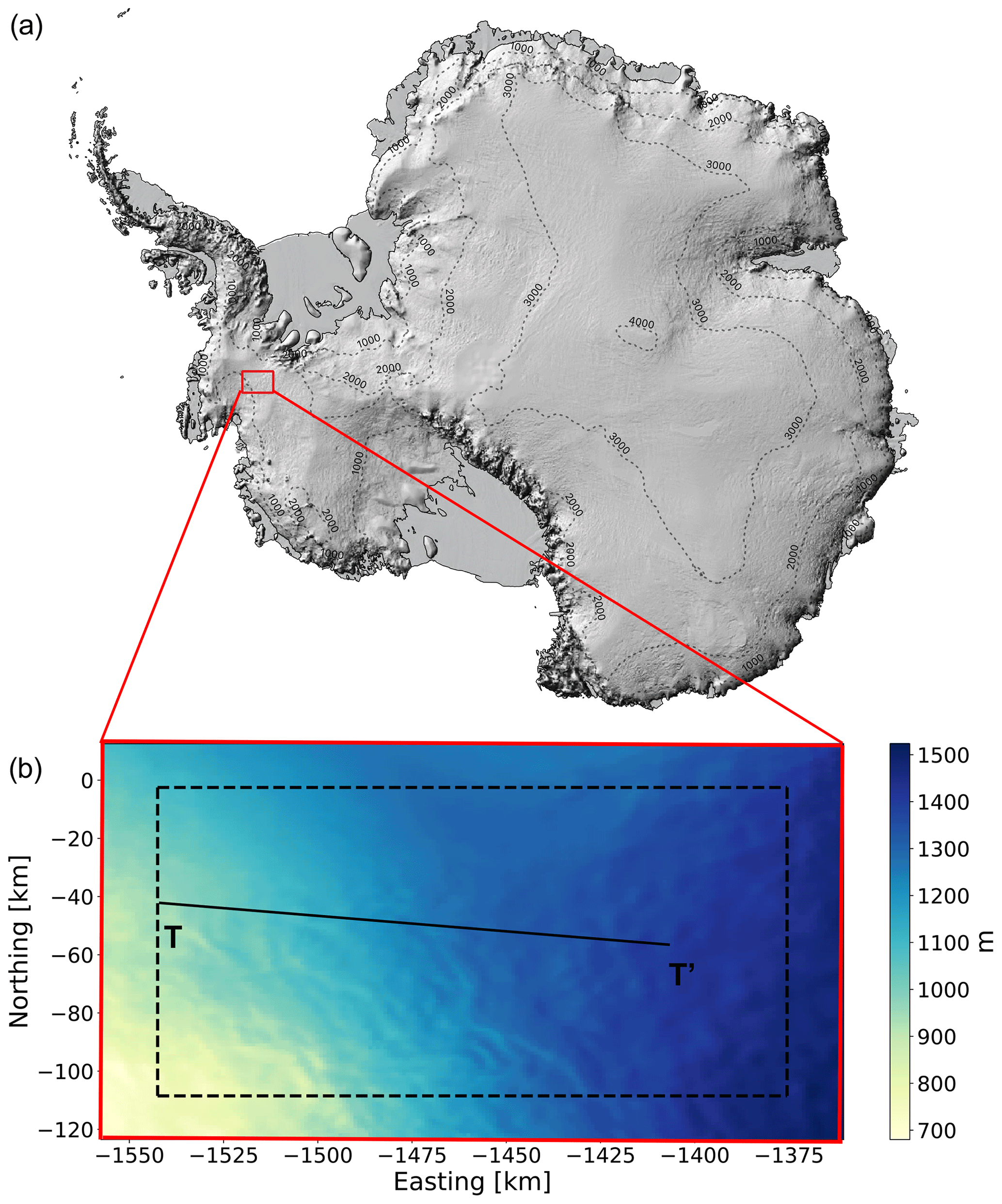
Figure 2Alpine3D modeling and analysis domains in the EPSG 3031 coordinate system. (a) The 198 km × 137 km Alpine3D modeling domain (red rectangle) is centered over the Pine Island Glacier basin in West Antarctica. (b) Surface topography of Alpine3D modeling (red) and analysis (black dashed) domains with the location of the 130 km observed SMB transect (black line, T–T′). Panel (a) was created using the Norwegian Polar Institute's Quantarctica package (Matsuoka et al., 2018).
2.6 Computational parallelization and benchmarking
To enable efficient numerical parallelization, the Alpine3D modeling framework supports a hybrid OpenMP–MPI implementation. For benchmarking, we perform calculations on a 1 km horizontal resolution 27 126 km2 domain (Sect. 2.5) using general-purpose compute nodes with 24 parallel CPUs per node. In the case of offline WindNinja wind speed and direction downscaling, we use one node (OpenMP, 24 CPUs) for 1 h per calendar year, resulting in a computational speed of 1130 km2 yr (CPU h)−1, whereas for Alpine3D calculations, we leverage four nodes (hybrid OpenMP–MPI, 96 total CPUs) for 18 h per calendar year, netting a computational speed of 16 km2 yr (CPU h)−1. WindNinja is therefore at least 1 order of magnitude computationally less expensive than Alpine3D, meaning that its added complexity is justified if downscaled SMB estimates are significantly improved.
2.7 Surface mass balance observations
To evaluate our SMB downscaling, we compare with a 130 km-long, radar-derived accumulation transect (Fig. 2b, black line T–T′) developed by Dattler et al. (2019a). This annual-averaged snow accumulation product captures spatial variability in along-track accumulation by tracking fluctuations in radar-derived firn isochrone thickness. Horizontal variations in thickness are then converted to mass using the Herron and Langway (1980) firn density model. At 25 km horizontal resolution, Dattler et al. (2019a) set the mean annual (1980–2017) accumulation to that of MERRA-2 atmospheric reanalysis, while at smaller scales, accumulation is modified by the combination of firn isochrone thickness and simulated firn density. This product intends to represent the annual-average SMB. However, because of the finite thickness of firn isochrones and spatially variable accumulation rates, the annual average is calculated over varying periods depending on the location. No quantitative uncertainty estimates are assigned to the absolute SMB observations; however, the authors report an average relative accumulation error of 0.02 %.
3.1 Impact of the wind downscaling method on simulated surface mass balance
To demonstrate the differences between downscaling techniques, we have downscaled MERRA-2 winds from the year 2015 using both the Liston and WindNinja (Sect. 2.2) algorithms to the 1 km Alpine3D grid (Fig. 3). WindNinja predicts a higher average wind speed than Liston (6.5 m s−1 vs. 6.1 m s−1) and is more consistent with MERRA-2 (6.6 m s−1), which can be explained by WindNinja's mass conservation solver and Liston's imposed terrain-weighting factor of 0.5–1.5 times the original interpolated value (Reynolds et al., 2021). Notably, both downscaling techniques predict local topography-driven wind speed variability not captured by MERRA-2; however, this variability is in the opposite phase, meaning that when WindNinja predicts relatively high wind speed, Liston predicts locally lower wind speed. Furthermore, WindNinja predicts 2–3 times larger local topography-driven wind speed variability than Liston, leading us to expect larger SMB variability in Alpine3D simulations forced with WindNinja winds compared to Liston-driven simulations. Likewise, because predicted wind speed accelerations are out of phase between the WindNinja and Liston downscaling methods, we anticipate the subsequent offline coupling with Alpine3D to predict opposite patterns of deposition and erosion. Note that our modeling domain (Sect. 2.5) lacks the necessary wind speed and direction observations required for a robust evaluation, and therefore we focus our evaluation on downscaled SMB, which ultimately integrates wind speed and direction and can be evaluated against observations (Sect. 2.7).
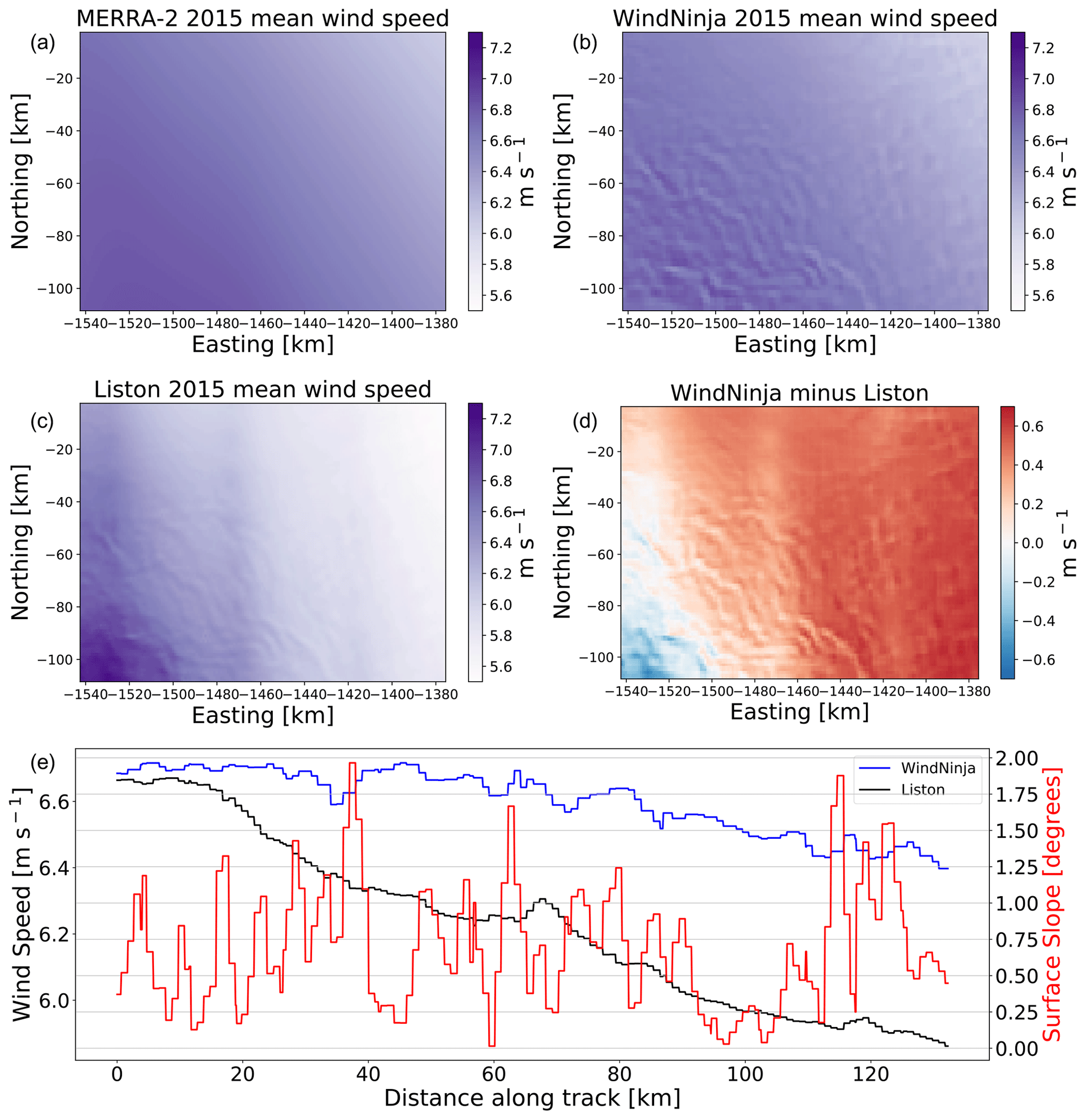
Figure 3Example of wind speed downscaling for the year 2015: (a) annual mean MERRA-2, (b) WindNinja, and (c) Liston 10 m wind speeds. (d) Annual mean WindNinja minus Liston wind speed. (e) Transect (T–T′ in Fig. 2b) of annual mean WindNinja and Liston wind speeds as well as transect surface slope.
Owing to the largely contrasting results between the WindNinja and Liston wind downscaling techniques, we have performed two 2015 Alpine3D simulations, one using WindNinja and one using Liston winds. As discussed above, the WindNinja-driven Alpine3D simulation exhibits larger SMB variability than the Liston-driven simulation (Fig. 4) because of larger wind speed variability in the former. Additionally, the WindNinja-driven Alpine3D simulation predicts SMB variability in phase with observations (slope = 0.26, p<0.001), whereas the Liston-driven simulation predicts SMB variability out of phase with observations (slope = −0.12, p<0.001). Because the offline coupling between the Liston downscaling algorithm and Alpine3D predicts SMB variability out of phase with observations, we determine that the Liston algorithm is not suitable for our application. Thus, moving forward, we only consider Alpine3D simulations driven by an offline coupling with WindNinja.
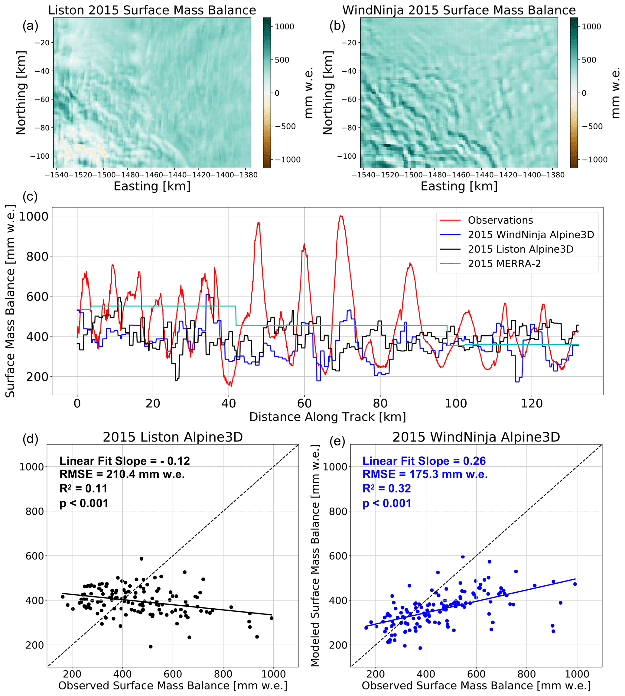
Figure 4Surface mass balance downscaling: (a) 2015 Liston and (b) WindNinja Alpine3D SMB. (c) Transect of observed (red), 2015 WindNinja Alpine3D (blue), Liston Alpine3D (black), and MERRA-2 (cyan) SMB. (d, e) Scatter plot of (d) 2015 Liston and (e) WindNinja Alpine3D SMB vs. observations.
3.2 Alpine3D downscaled surface mass balance
Given the demonstrated performance advantage of using the offline WindNinja coupling with Alpine3D (Sect. 3.1), we further this analysis by evaluating a 6-year-long Alpine3D simulation using WindNinja (2015–2020). By comparing with an approximately 130 km-long observational transect, we found that, based on the simulated 2015–2020 mean annual SMB, Alpine3D correctly predicts the relative locations of peaks and troughs in observed SMB. Under the assumption that the modeled and observed SMBs are linearly related and thus that R2 provided by the linear regression equals the variance explained, we find that Alpine3D SMB gives an additional 24 % variance explained compared to MERRA-2 (31 % (17 %–47 % 95 % confidence interval) vs. 7 % (2 %–15 % 95 % confidence interval), Fig. 5). In particular, Alpine3D appears to improve over MERRA-2 SMB predictions as indicated by a reduction in root mean squared error (152.7 vs. 176.1 ). Despite improving over MERRA-2 (slope = 0.13, p=0.003), Alpine3D still underestimates the magnitude of observed SMB variability, as indicated by the linear fit slope being less than 1 (slope = 0.25, p<0.001).
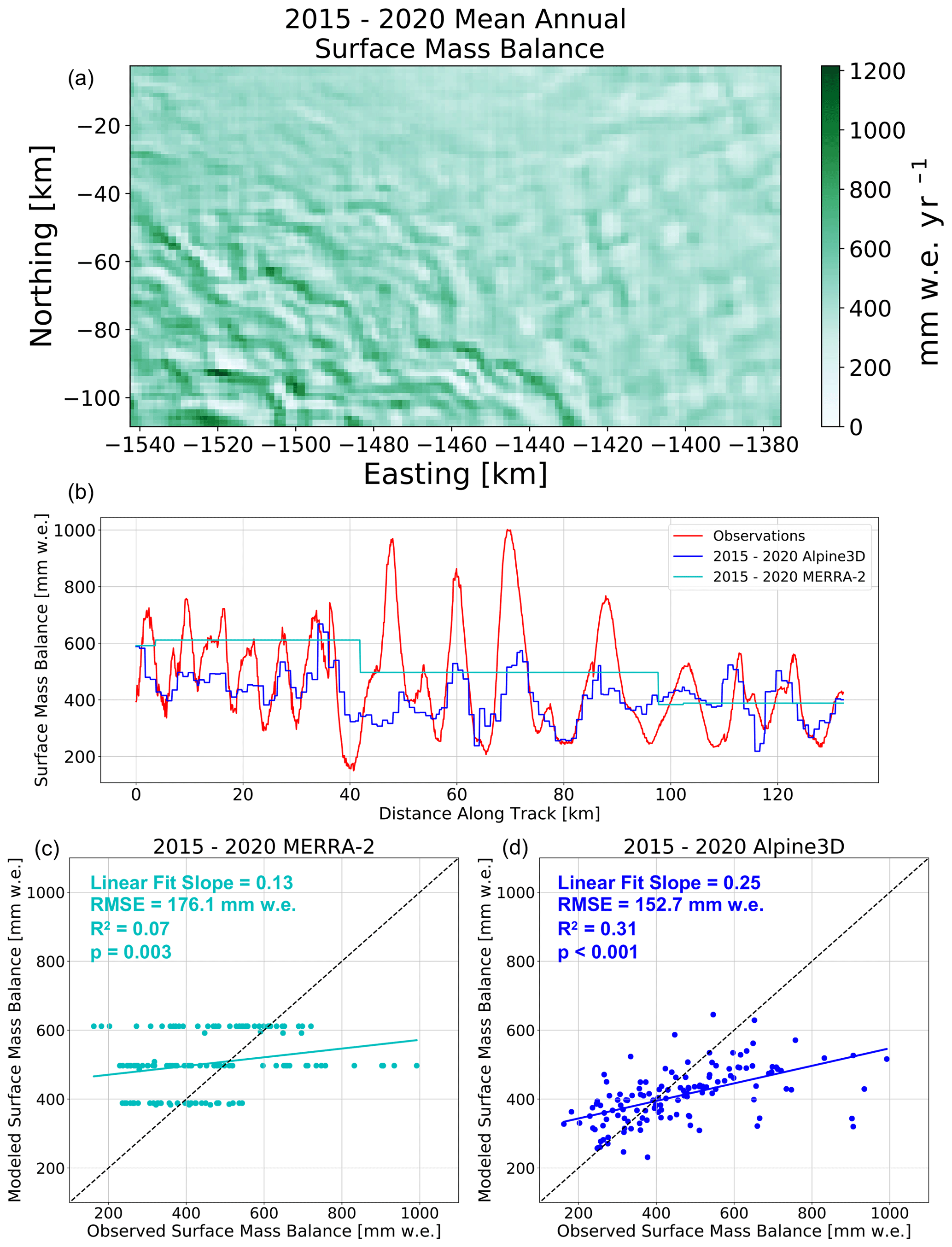
Figure 5Surface mass balance downscaling: (a) 2015–2020 Alpine3D SMB. (b) Transect of observed (red), 2015–2020 mean Alpine3D (blue), and MERRA-2 (cyan) SMB. (c, d) Scatter plot of (c) 2015–2020 MERRA-2 and (d) Alpine3D SMB vs. observations.
Generally speaking, Alpine3D correctly predicts the location of deposition and erosion, as evidenced by the relative positioning of peaks and troughs in SMB. However, the simulated amplitude of deposition and erosion is underestimated when compared to observations. This underestimation could potentially be ameliorated by decreasing the fetch length and therefore increasing the saltation mass flux, although we show in Sect. 3.6 that doing so results in locally excessive erosion and, in fact, negative SMB. While most peaks and troughs in SMB are captured by Alpine3D, some are missed, e.g., near 45 km on the transect in Fig. 5b. Several processes likely contribute to this significant model error; however, the primary driver is a lack of terrain-driven wind acceleration at this point of the transect (Fig. 3e). Despite indications that this area has some of the largest SMB variability within the transect, surface slopes in the DEM are comparatively modest (, Fig. 3). Without significant surface slopes, the downscaled wind speeds are relatively homogeneous, leading Alpine3D to miss the corresponding observed SMB variability. This relatively homogeneous wind field in the presence of large observed accumulation gradients can be potentially attributed to a combination of terrain representation errors in the DEM and process representation errors and simplifications within the WindNinja downscaling algorithms. Furthermore, it is worth noting that, over the length of the transect, MERRA-2 2015–2020 mean annual SMB exceeds that of observations (504 and 461 ), indicating that the 2015–2020 simulated SMB exceeded the 1980–2017 MERRA-2 mean annual SMB (Sect. 2.7). Despite this, mean Alpine3D downscaled SMB over the transect (410 ) is less than both observations and MERRA-2. The discrepancy between MERRA-2 and Alpine3D along the transect is most likely explained by net divergence of saltating snow out of the analysis domain (Fig. 2), resulting in less mass available for accumulation along the transect. Since wind speeds generally increase from the top right to the bottom left over the model domain, some net divergence over the transect may also occur. Because the observations are deliberately forced to have the same mean as MERRA-2 (Sect. 2.7), we are unable to properly evaluate this predicted discrepancy against measurements.
3.3 Link between topography, surface winds, and drifting snow redistribution
Intuitively, Alpine3D is designed to preferentially erode snow in wind-exposed areas and redeposit it downwind in wind-sheltered zones. This is primarily achieved through the offline coupling between WindNinja and Alpine3D. In areas with spatially varying surface slopes, WindNinja adjusts wind speed and direction to account for mechanical effects of terrain on the flow (Fig. 6). In the case of the transect (location shown in Fig. 2), surface slopes are relatively modest but regularly vary between 0.25 and 2.0∘. Ultimately, this rolling terrain leads WindNinja to simulate equally subtle wind speed variations up to approximately 0.1 m s−1. The end result is enhanced erosion (0–250 ) of snow in relatively windy areas and subsequent deposition (up to 125 ) in less windy areas. Expanding this analysis to our entire domain, we see that rolling topography drives spatially variable patterns of deposition and erosion (Fig. 6d). On average, wind-driven transport processes remove 50 from the analysis domain, while local values of erosion and deposition range from −514 to 690 . Overall, deposition and erosion processes modify snow accumulation with an average magnitude of 89 , which corresponds to 23 % of mean annual accumulation.
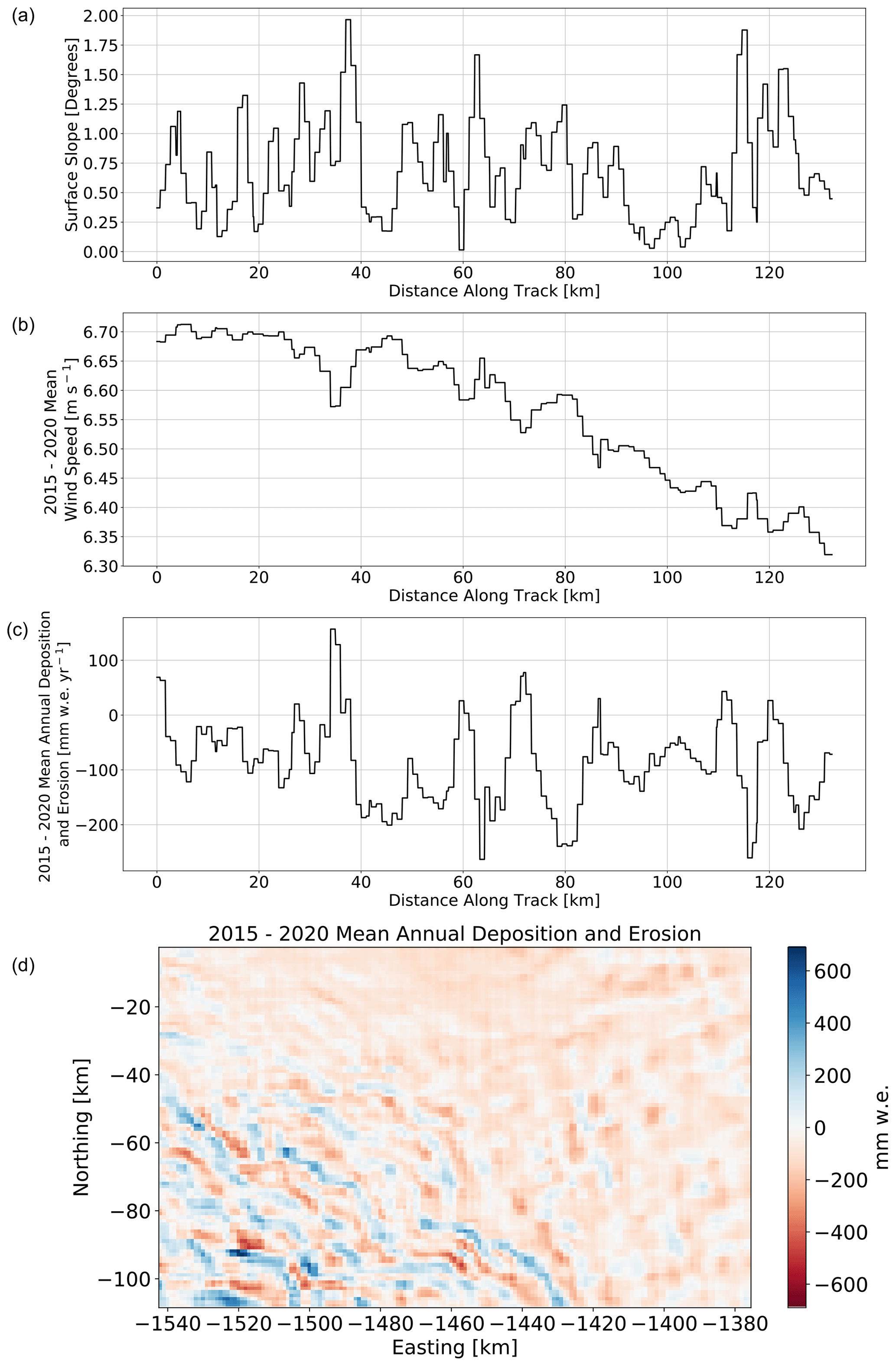
Figure 6Connection between topography and snow redistribution. (a) Transect of surface slope, (b) 2015–2020 mean 10 m wind speed, and (c) 2015–2020 mean deposition and erosion. (d) Map of 2015–2020 mean annual deposition and erosion.
3.4 Link between density and deposition and erosion
Altimetry-based ice sheet mass balance retrievals rely on firn density products to perform volume-to-mass conversions. Thus, accurate firn models are necessary for reliable local-, regional-, and continental-scale mass balance assessments. Because erosion exposes older and denser snow layers while also coinciding with areas of elevated wind speed, one could plausibly expect Alpine3D to predict areas with net erosion to coincide with relatively high surface density. Interestingly, we show that this is not the case. Instead, Alpine3D predicts wind-driven compaction to be the dominant process, whereby eroded snow particles experience densification via fragmentation and rounding on their way to subsequent deposition (Vionnet et al., 2012). By comparing 2015–2020 mean annual Alpine3D surface density (defined as the mean of the top 10 cm) with deposition and erosion, we find that the two are correlated (R=0.74, Fig. 7). Although this positive correlation is not directly verified by in situ observations, Grima et al. (2014) found a similar correlation between surface density and local SMB perturbations over Thwaites Glacier. If for the moment we assume this model result is correct, then the accumulation product compiled by Dattler et al. (2019a) most likely underestimates SMB spatial variability because of the constant surface density assumption used to initialize their firn model. Likewise, in the case of repeat altimetry, we can deduce that variable surface height change in the vicinity of rolling topography may represent more enhanced mass change variability than we might otherwise expect with a homogeneous density field. Overall, these findings should be interpreted with caution as they are not yet directly verified by observations but likewise warrant the consideration of detailed firn density products when interpreting airborne snow accumulation radar and satellite altimetry.
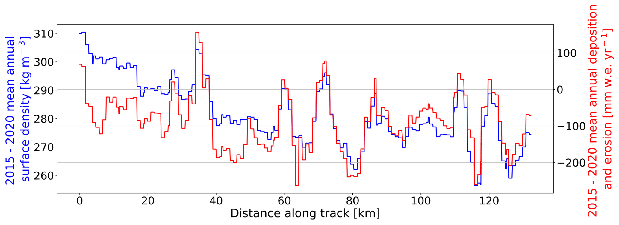
Figure 7Connection between deposition and erosion and surface density (defined as the mean of the top 10 cm). Transect of 2015–2020 mean Alpine3D surface density (blue) and annual deposition and erosion (red).
3.5 Impact of horizontal model resolution on downscaled SMB
Depending on the Alpine3D downscaling application, it may be desirable to decrease horizontal resolution in favor of larger domains or longer simulations. We also want to test the sensitivity of the numerics used in Alpine3D to the spatial resolution. In order to inform future modeling studies which will inevitably weigh computational costs against spatial and temporal detail, here we describe results from a 1 and 3 km horizontal resolution 2015 Alpine3D simulation. Owing primarily to a reduced number of individual Alpine3D grid cells, the 3 km simulation requires only 10 % of the 1 km simulation's computational resources (Sect. 2.6).
Generally speaking, both simulations capture observed topographic-driven variability in SMB (Fig. 8); however, the 1 km simulation predicts 40 % larger SMB variability than the 3 km simulation. This finding can be explained by the relatively smoother terrain in the 3 km simulation and consequently reduced terrain-induced wind speed variability. Reduced wind speed variations across subtle topography ultimately reduced the magnitude of deposition and erosion, leading to a more homogeneous SMB field (Fig. 8a vs. Fig. 8b). That said, the 3 km simulation explains an additional 5 % variance of observed accumulation variability compared to the 1 km simulation, all while reducing the RMSE by 8 (Table 1). These improved statistics could be explained by reduced wind-transport divergence in the 3 km simulation (−48.8 vs. −51.4 ) and subsequent reduction of the mean bias. However, given that the observed accumulation mean is controlled by MERRA-2 (Sect. 2.7), caution should be taken in interpreting the absolute value of observations. Overall, these findings suggest that the 1 and 3 km simulations perform similarly, implying that the Alpine3D framework can be applied at horizontal resolutions greater than 1 km without unacceptable degradation of performance. Furthermore, because performance at 3 km horizontal resolution is comparable to that of 1 km, future Alpine3D applications can consider increasing grid spacing up to 3 km in order to expand the spatial and temporal bounds of their simulation.
Table 1Linear regression statistics for different choices of horizontal resolution. Coefficient of determination (R2), root mean squared error (RMSE), and linear regression slope for 2015 Alpine3D simulations with 1 and 3 km horizontal resolution against observations.
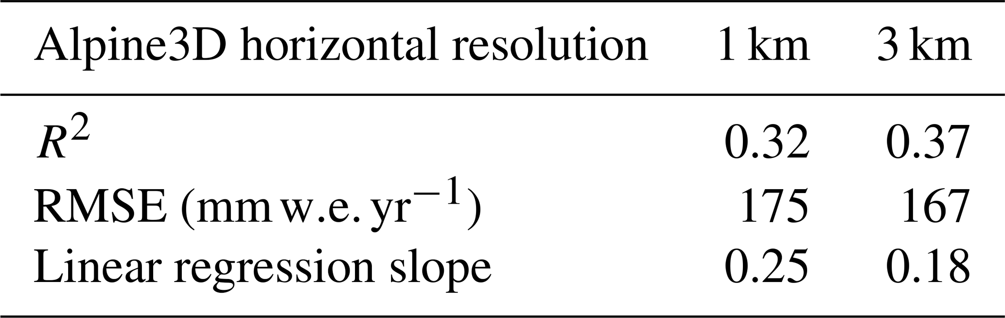
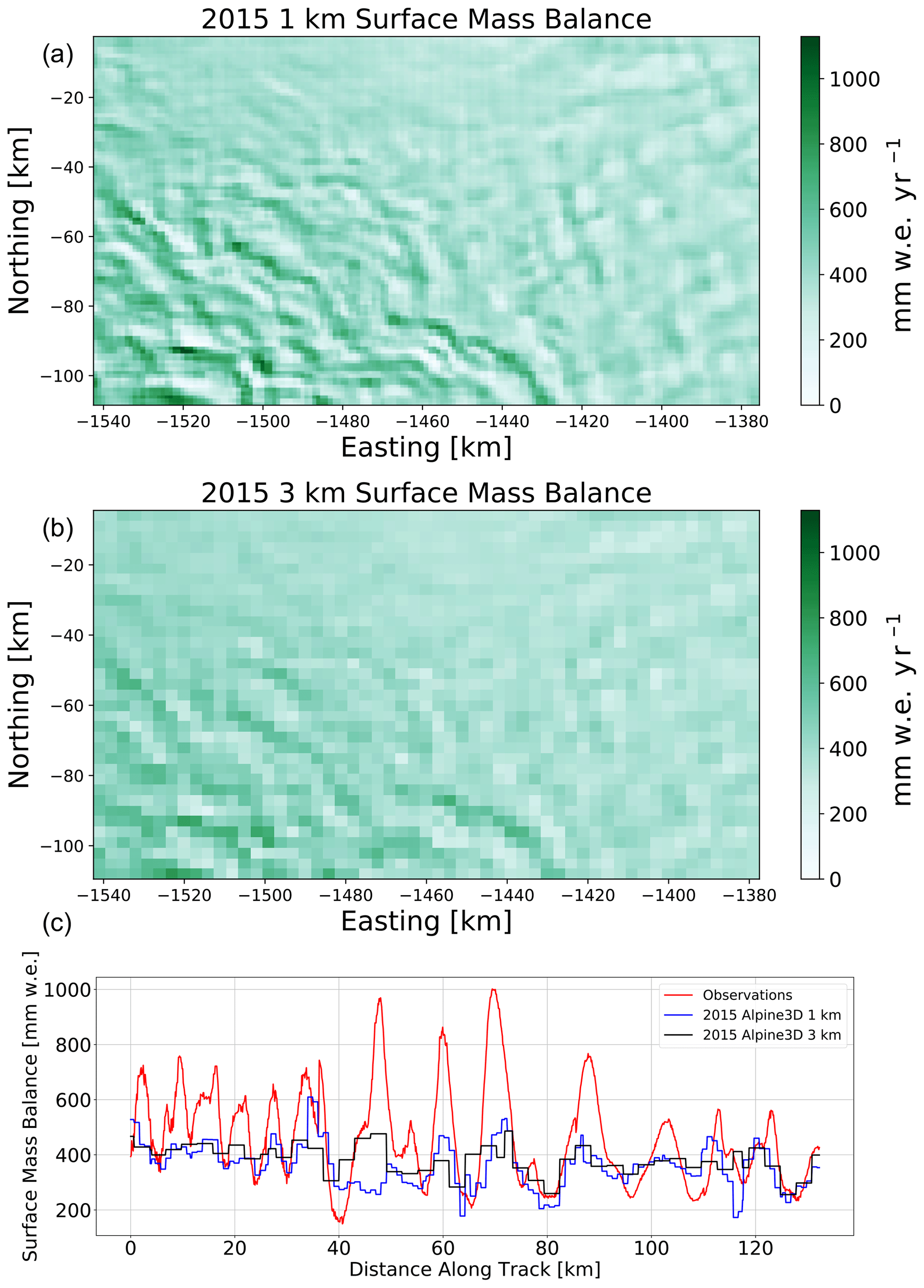
Figure 8Connection between horizontal resolution and simulated SMB; 2015 simulated SMB with (a) 1 and (b) 3 km horizontal resolution. (c) Transect of observed (red) and simulated SMB with 1 (blue) and 3 km (black) horizontal resolution.
3.6 Sensitivity to prescribed fetch length
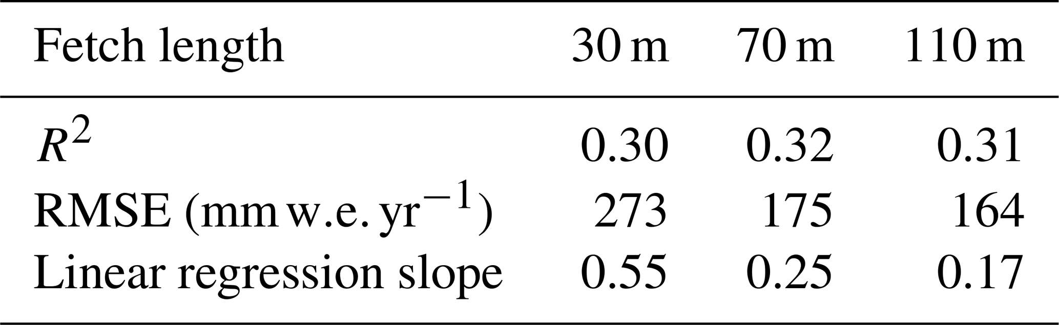
As indicated in Sect. 2.3, the SNOWPACK fetch length is an uncertain tuning parameter that controls the magnitude of the saltation mass flux. Furthermore, because no suitable observations or theoretical frameworks firmly suggest which value of fetch length to choose, here we present results from a sensitivity study designed to quantify the effect of varying the fetch length between 30, 70, and 110 m. As expected, progressively increasing the fetch length from 30 to 110 m decreases the magnitude of deposition and erosion and consequently the spatial variability of the 2015 Alpine3D-simulated surface mass balance (Fig. 9). Note that, by decreasing the fetch length, we increase the simulated SMB variability to be more in line with observations. However, decreasing the fetch length to 30 m results in unrealistically strong erosion, as indicated by negative SMB values in 4.2 % of grid cells. In fact, the 30 m fetch length simulation produces a larger RMSE than both the 70 and 110 m simulations (273, 175, and 164 , respectively, Table 2).
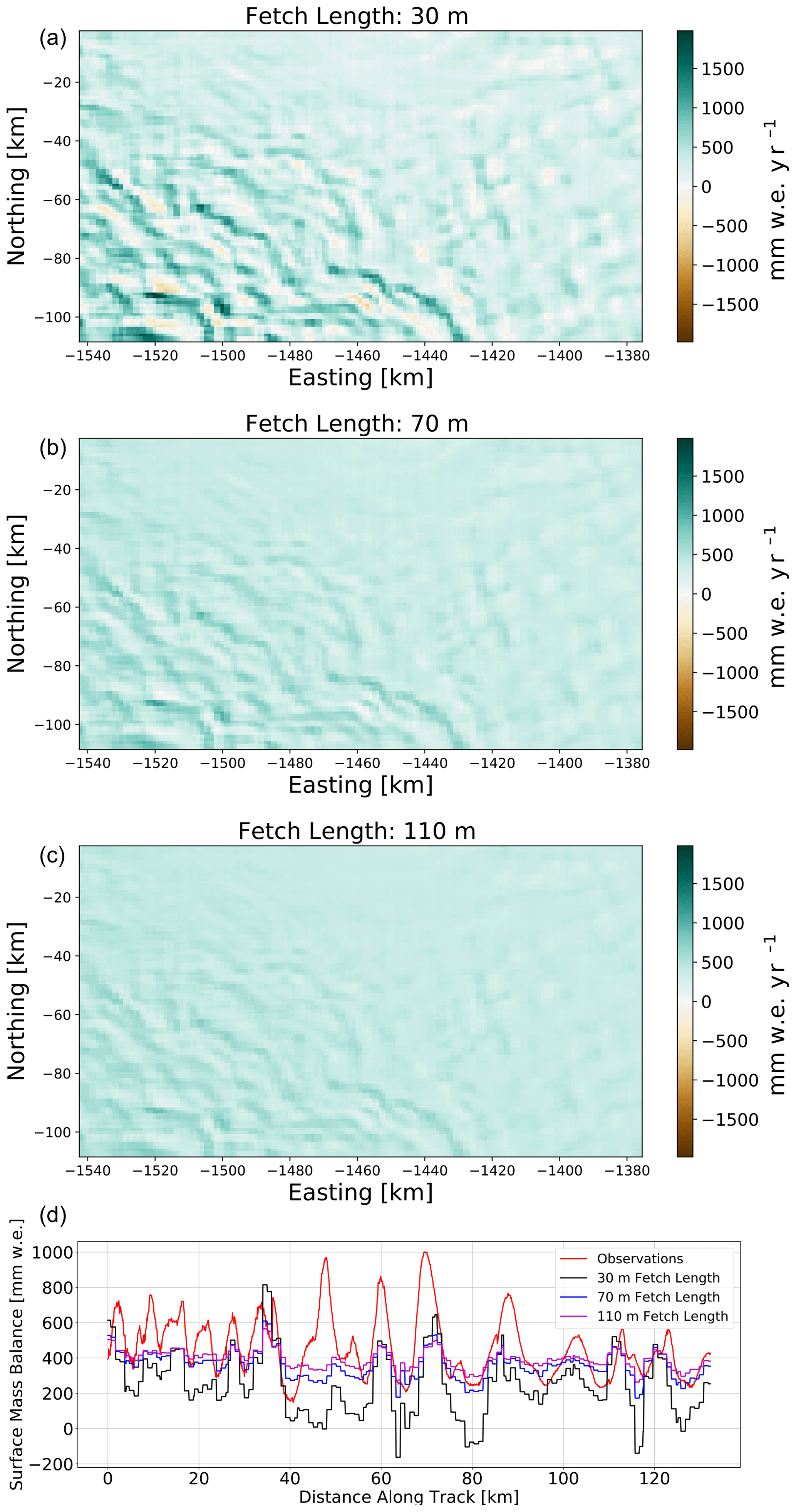
Figure 9Connection between prescribed fetch length and simulated SMB; 2015 simulated SMB with (a) 30, (b) 70, and (c) 110 m fetch lengths. (d) Transect of observed (red) and simulated SMB with 30 (black), 70 (blue), and 110 m (magenta) fetch lengths.
Despite the relatively limited breadth of our fetch length ensemble, we observe a notable tradeoff. As we decrease fetch length, simulated SMB variability approaches that of observations (as indicated by linear regression slopes in Table 2) while also increasing typical model errors (RMSE in Table 2). We have therefore identified a potential shortcoming of our Alpine3D downscaling framework, namely, that optimizing the fetch length parameter does not result in uniformly improved results. For purely pragmatic reasons, in this study we retain the fetch length approach by choosing a middle-ground value of 70 m. Nevertheless, in future model development exercises it would be useful to drop this reliance on fetch length and instead focus on diagnosing the locally eroded mass purely from simulated snow characteristics and surface wind stress.
Table 2Linear regression statistics for different choices of fetch length. R2, RMSE, and linear regression slope for 2015 Alpine3D simulations with 30, 70, and 110 m fetch lengths against observations.
3.7 Simulation without wind redistribution of snow
Finally, we performed a simulation without activating the newly developed module for wind redistribution of snow (Fig. 10) while keeping the WindNinja downscaling for wind as well as the downscaling approaches for the other variables. We find that, in this case, the SMB field (Fig. 10a) is strongly dominated by the large-scale gradient in SMB resulting from the MERRA-2 forcing data while lacking the small-scale spatial variability found in the simulation with drifting snow shown in Fig. 4b. It illustrates that the Alpine3D simulation does not create any substantial small-scale variability in SMB that could arise from other processes. For example, wind speed also controls surface sublimation, but the effect on SMB is not noticeable on larger scales. We conclude that the simulations including the wind redistribution of snow attribute virtually all of the spatial heterogeneity in SMB to snow redistribution processes by the wind (Fig. 4c, d).
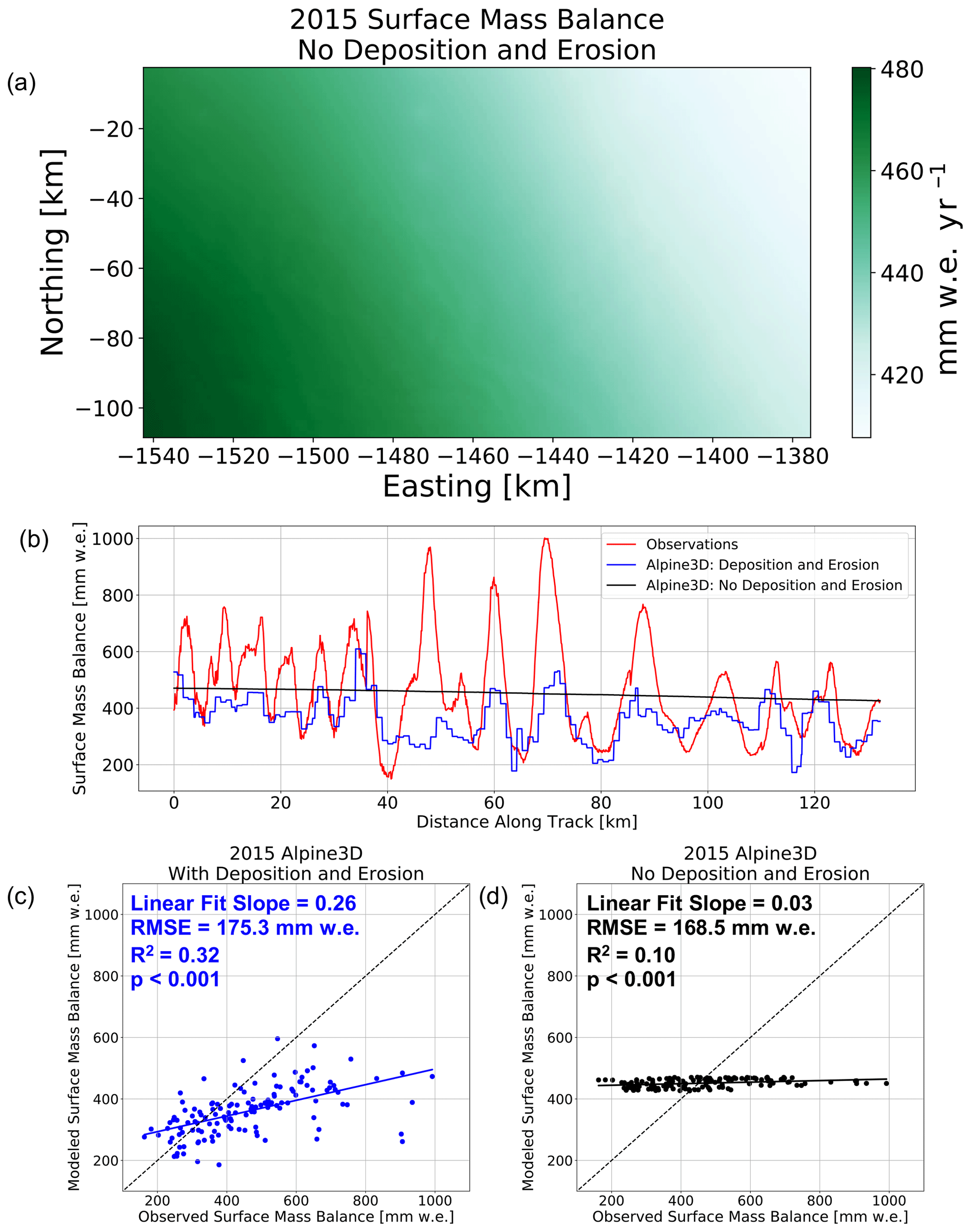
Figure 10Comparing the simulation with and without wind redistribution of snow for the year 2015. (a) 2015 Alpine3D SMB without wind redistribution of snow, (b) transect of observed SMB (red), 2015 Alpine3D with wind redistribution (blue), and 2015 Alpine3D without wind redistribution (black) SMB. (c, d) Scatter plot of (c) 2015 with wind redistribution and (d) 2015 without wind redistribution vs. observations.
The primary way ice sheets accumulate mass is through net snow accumulation at the ice sheet surface. SMB quantifies the balance between processes which accumulate and ablate mass at the surface of ice sheets. Throughout the last 2 decades, regional climate models have been progressively developed to simulate large-scale ice sheet SMB fields. However, recent advancements in observational capabilities (e.g., repeat satellite altimetry and airborne snow radar) indicate that SMB varies predictably in the presence of rolling topography. Despite the importance of capturing this SMB variability for assigning a mass change to repeat altimetry measurements, regional climate models are not capable of resolving this variability. To begin to close the gap between observations and existing regional climate models and therefore improve local SMB estimates and support interpretation of repeat altimetry, we have expanded upon the Alpine3D framework in order to dynamically downscale Antarctic SMB. In our implementation of Alpine3D, we leverage MeteoIO and WindNinja software to downscale meteorology onto the native Alpine3D grid. At each grid cell, the SNOWPACK snow model is used to diagnose snow properties, including density, temperature, grain size, and other snow microstructure parameters. With this information, SNOWPACK calculates a saltation mass flux for each time step and then sends this information to Alpine3D, where horizontal snow redistribution is treated as a two-dimensional advection problem. WindNinja downscaling results suggest that rolling topographies with surface slopes between 0.25 and 2.0∘ are responsible for subtle terrain-induced mechanical effects that vary mean wind speeds by 0.1 m s−1. These wind speed perturbations ultimately drive spatially variable patterns of deposition and erosion whose mean magnitude corresponds to 23 % of mean annual accumulation.
By comparing 2015–2020 mean annual SMB downscaling results over a portion of Pine Island Glacier, West Antarctica, to a 130 km-long observational SMB transect, we found that, when compared to MERRA-2, Alpine3D reduces typical SMB errors by 23.4 (13 %) and increases variance explained by 24 %. Furthermore, we show that Alpine3D produces a similarly skillful downscaled SMB product when run at 3 km horizontal resolution. This suggests that Alpine3D can be run at a coarser resolution than what is primarily shown in this study (1 km horizontal resolution), therefore considerably reducing computational cost. Finally, despite the promising downscaling results presented in this study, Alpine3D still relies on the fetch length tuning parameter to scale the saltation mass flux. We have shown that the magnitudes of deposition and erosion, and consequently SMB, are sensitive to the choice of fetch length. Because it is at the very least difficult, and quite likely impossible, to uniformly optimize the fetch length, we suggest that future studies migrate towards diagnosing the saltation mass flux purely from known quantities including snow properties and surface wind stress. Furthermore, we note that our implementation makes important simplifications by neglecting drifting and blowing snow sublimation as well as horizontal redistribution by way of suspension. In regions where these processes are significant drivers of local SMB, future downscaling efforts would likely be improved by inclusion of these processes in Alpine3D.
MeteoIO, SNOWPACK, and Alpine3D are software published under the GNU LGPLv3 license by the WSL Institute for Snow and Avalanche Research SLF, Davos, Switzerland, at https://gitlabext.wsl.ch/snow-models (Wagner et al., 2022). The repository used to develop the versions of MeteoIO, SNOWPACK, and Alpine3D used in this study can be accessed at https://github.com/snowpack-model/snowpack (last access: 4 June 2023), with the exact version corresponding to commit f023b9f archived at https://doi.org/10.5281/zenodo.5914787 (Wever et al., 2022b). MERRA-2 atmospheric reanalysis is available at https://gmao.gsfc.nasa.gov/reanalysis/MERRA-2/ (last access: 4 June 2023; Gelaro et al., 2017) and can be retrieved and processed using our workflow available at https://github.com/EricKeenan/download_MERRA2 (last access: 4 June 2023) and archived at https://doi.org/10.5281/zenodo.4560825 (Keenan, 2021). WindNinja source code is hosted at https://github.com/firelab/windninja (last access: 4 June 2023), while the version used in this study is permanently archived at https://doi.org/10.5281/zenodo.4474633 (Shannon et al., 2021). Software used to produce the numerical simulations, analyses, and figures presented in this study is archived at https://doi.org/10.5281/zenodo.5914751 (Keenan, 2022a) and https://doi.org/10.5281/zenodo.5914727 (Keenan, 2022b). Airborne snow accumulation radar data used in this study are archived at https://doi.org/10.5281/zenodo.3534315 (Dattler et al., 2019b).
All the authors contributed to experimental design, analysis, and manuscript preparation. Eric Keenan carried out Alpine3D simulations, performed the analysis, and produced the figures. EK and NW both contributed to Alpine3D model development.
The contact author has declared that none of the authors has any competing interests.
Publisher's note: Copernicus Publications remains neutral with regard to jurisdictional claims in published maps and institutional affiliations.
The authors thank Charles Amory and an anonymous reviewer for their thoughtful comments which helped to improve the manuscript considerably. This work utilized the RMACC Summit supercomputer, which is supported by the National Science Foundation (awards ACI-1532235 and ACI-1532236), the University of Colorado Boulder, and Colorado State University. The Summit supercomputer is a joint effort of the University of Colorado Boulder and Colorado State University. Data storage supported by the University of Colorado Boulder “PetaLibrary”.
This research has been supported by the National Aeronautics and Space Administration (grant no. 80NSSC18K0201).
This paper was edited by Fabien Maussion and reviewed by Charles Amory and one anonymous referee.
Alley, R. B. and Koci, B. R.: Recent Warming in Central Greenland?, Ann. Glaciol., 14, 6–8, https://doi.org/10.3189/S0260305500008144, 1990. a
Amory, C., Gallée, H., Naaim-Bouvet, F., Favier, V., Vignon, E., Picard, G., Trouvilliez, A., Piard, L., Genthon, C., and Bellot, H.: Seasonal Variations in Drag Coefficient over a Sastrugi-Covered Snowfield in Coastal East Antarctica, Bound.-Lay. Meteorol., 164, 107–133, https://doi.org/10.1007/s10546-017-0242-5, 2017. a
Amory, C., Kittel, C., Le Toumelin, L., Agosta, C., Delhasse, A., Favier, V., and Fettweis, X.: Performance of MAR (v3.11) in simulating the drifting-snow climate and surface mass balance of Adélie Land, East Antarctica, Geosci. Model Dev., 14, 3487–3510, https://doi.org/10.5194/gmd-14-3487-2021, 2021. a, b, c, d
Bartelt, P. and Lehning, M.: A physical SNOWPACK model for the Swiss avalanche warning Part I: numerical model, Cold Reg. Sci. Technol., 35, https://doi.org/10.1016/S0165-232X(02)00074-5, 2002. a
Bavay, M. and Egger, T.: MeteoIO 2.4.2: a preprocessing library for meteorological data, Geosci. Model Dev., 7, 3135–3151, https://doi.org/10.5194/gmd-7-3135-2014, 2014. a, b
Bintanja, R.: Snowdrift suspension and atmospheric turbulence. Part I: Theoretical background and model description, Bound.-Lay. Meteorol., 95, 343–368, https://doi.org/10.1023/A:1002676804487, 2000. a
Clifton, A., Rüedi, J.-D., and Lehning, M.: Snow saltation threshold measurements in a drifting-snow wind tunnel, J. Glaciol., 52, 585–596, https://doi.org/10.3189/172756506781828430, 2006. a
Comola, F., Gaume, J., Kok, J. F., and Lehning, M.: Cohesion‐Induced Enhancement of Aeolian Saltation, Geophys. Res. Lett., 46, 5566–5574, https://doi.org/10.1029/2019GL082195, 2019a. a
Comola, F., Giometto, M. G., Salesky, S. T., Parlange, M. B., and Lehning, M.: Preferential Deposition of Snow and Dust Over Hills: Governing Processes and Relevant Scales, J. Geophys. Res.-Atmos., 124, 7951–7974, https://doi.org/10.1029/2018JD029614, 2019b. a
Courant, R., Friedrichs, K., and Lewy, H.: Über die partiellen Differenzengleichungen der mathematischen Physik, Math. Ann., 100, 32–74, https://doi.org/10.1007/BF01448839, 1928. a
Dattler, M. E., Lenaerts, J. T. M., and Medley, B.: Significant Spatial Variability in Radar‐Derived West Antarctic Accumulation Linked to Surface Winds and Topography, Geophys. Res. Lett., 46, 13126–13134, https://doi.org/10.1029/2019GL085363, 2019a. a, b, c, d, e, f, g
Dattler, M. E., Lenaerts, J. T. M., and Medley, B.: Antarctic Snow Radar-Derived Relative Accumulation Product, Zenodo [data set], https://doi.org/10.5281/zenodo.3534315, 2019b. a
Forthofer, J. M., Butler, B. W., and Wagenbrenner, N. S.: A comparison of three approaches for simulating fine-scale surface winds in support of wildland fire management. Part I. Model formulation and comparison against measurements, Int. J. Wildland Fire, 23, 969, https://doi.org/10.1071/WF12089, 2014. a
Gelaro, R., McCarty, W., Suárez, M. J., Todling, R., Molod, A., Takacs, L., Randles, C. A., Darmenov, A., Bosilovich, M. G., Reichle, R., Wargan, K., Coy, L., Cullather, R., Draper, C., Akella, S., Buchard, V., Conaty, A., da Silva, A. M., Gu, W., Kim, G.-K., Koster, R., Lucchesi, R., Merkova, D., Nielsen, J. E., Partyka, G., Pawson, S., Putman, W., Rienecker, M., Schubert, S. D., Sienkiewicz, M., and Zhao, B.: The Modern-Era Retrospective Analysis for Research and Applications, Version 2 (MERRA-2), J. Climate, 30, 5419–5454, https://doi.org/10.1175/JCLI-D-16-0758.1, 2017 (data available at: https://gmao.gsfc.nasa.gov/reanalysis/MERRA-2/, last access: 4 June 2023). a, b
Gerber, F., Lehning, M., Hoch, S. W., and Mott, R.: A close-ridge small-scale atmospheric flow field and its influence on snow accumulation, J. Geophys. Res.-Atmos., 122, 7737–7754, https://doi.org/10.1002/2016JD026258, 2017. a, b
Grima, C., Blankenship, D. D., Young, D. A., and Schroeder, D. M.: Surface slope control on firn density at Thwaites Glacier, West Antarctica: Results from airborne radar sounding: SURFACE SLOPE CONTROL ON FIRN DENSITY, Geophys. Res. Lett., 41, 6787–6794, https://doi.org/10.1002/2014GL061635, 2014. a
Gromke, C., Horender, S., Walter, B., and Lehning, M.: Snow particle characteristics in the saltation layer, J. Glaciol., 60, 431–439, https://doi.org/10.3189/2014JoG13J079, 2014. a
Groot Zwaaftink, C. D., Cagnati, A., Crepaz, A., Fierz, C., Macelloni, G., Valt, M., and Lehning, M.: Event-driven deposition of snow on the Antarctic Plateau: analyzing field measurements with SNOWPACK, The Cryosphere, 7, 333–347, https://doi.org/10.5194/tc-7-333-2013, 2013. a, b
Hames, O., Jafari, M., Wagner, D. N., Raphael, I., Clemens-Sewall, D., Polashenski, C., Shupe, M. D., Schneebeli, M., and Lehning, M.: Modeling the small-scale deposition of snow onto structured Arctic sea ice during a MOSAiC storm using snowBedFoam 1.0., Geosci. Model Dev., 15, 6429–6449, https://doi.org/10.5194/gmd-15-6429-2022, 2022. a
Helbig, N.: Application of the radiosity approach to the radiation balance in complex terrain, PhD thesis, University of Zurich, Switzerland, https://doi.org/10.5167/UZH-30798, 2009. a
Herron, M. M. and Langway, C. C.: Firn Densification: An Empirical Model, J. Glaciol., 25, 373–385, https://doi.org/10.3189/S0022143000015239, 1980. a
Kausch, T., Lhermitte, S., Lenaerts, J. T. M., Wever, N., Inoue, M., Pattyn, F., Sun, S., Wauthy, S., Tison, J.-L., and van de Berg, W. J.: Impact of coastal East Antarctic ice rises on surface mass balance: insights from observations and modeling, The Cryosphere, 14, 3367–3380, https://doi.org/10.5194/tc-14-3367-2020, 2020. a, b
Keenan, E.: EricKeenan/download_MERRA2: Download MERRA-2 (v1.0.0), Zenodo [code], https://doi.org/10.5281/zenodo.4560825, 2021. a
Keenan, E.: EricKeenan/SNOWPACK_WAIS: Initial release of SNOWPACK_WAIS (v1.0.0), Zenodo [code], https://doi.org/10.5281/zenodo.5914751, 2022a. a
Keenan, E.: EricKeenan/antarctic-windninja: Initial release of antarctic-windninja (v1.0.0), Zenodo [code], https://doi.org/10.5281/zenodo.5914727, 2022b. a
Keenan, E., Wever, N., Dattler, M., Lenaerts, J. T. M., Medley, B., Kuipers Munneke, P., and Reijmer, C.: Physics-based SNOWPACK model improves representation of near-surface Antarctic snow and firn density, The Cryosphere, 15, 1065–1085, https://doi.org/10.5194/tc-15-1065-2021, 2021. a, b, c, d, e, f, g, h, i, j, k
Lawrence, D. M., Fisher, R. A., Koven, C. D., Oleson, K. W., Swenson, S. C., Bonan, G., Collier, N., Ghimire, B., Kampenhout, L., Kennedy, D., Kluzek, E., Lawrence, P. J., Li, F., Li, H., Lombardozzi, D., Riley, W. J., Sacks, W. J., Shi, M., Vertenstein, M., Wieder, W. R., Xu, C., Ali, A. A., Badger, A. M., Bisht, G., Broeke, M., Brunke, M. A., Burns, S. P., Buzan, J., Clark, M., Craig, A., Dahlin, K., Drewniak, B., Fisher, J. B., Flanner, M., Fox, A. M., Gentine, P., Hoffman, F., Keppel‐Aleks, G., Knox, R., Kumar, S., Lenaerts, J., Leung, L. R., Lipscomb, W. H., Lu, Y., Pandey, A., Pelletier, J. D., Perket, J., Randerson, J. T., Ricciuto, D. M., Sanderson, B. M., Slater, A., Subin, Z. M., Tang, J., Thomas, R. Q., Val Martin, M., and Zeng, X.: The Community Land Model Version 5: Description of New Features, Benchmarking, and Impact of Forcing Uncertainty, J. Adv. Model. Earth Sy., 11, 4245–4287, https://doi.org/10.1029/2018MS001583, 2019. a
Lehning, M. and Fierz, C.: Assessment of snow transport in avalanche terrain, Cold Reg. Sci. Technol., 51, 240–252, https://doi.org/10.1016/j.coldregions.2007.05.012, 2008. a, b
Lehning, M., Bartelt, P., Brown, B., and Fierz, C.: A physical SNOWPACK model for the Swiss avalanche warning Part III: meteorological forcing, thin layer formation and evaluation, Cold Reg. Sci. Technol., 35, https://doi.org/10.1016/S0165-232X(02)00072-1, 2002a. a
Lehning, M., Bartelt, P., Brown, B., Fierz, C., and Satyawali, P.: A physical SNOWPACK model for the Swiss avalanche warning Part II. Snow microstructure, Cold Reg. Sci. Technol., 35, https://doi.org/10.1016/S0165-232X(02)00073-3, 2002b. a
Lehning, M., Völksch, I., Gustafsson, D., Nguyen, T. A., Stähli, M., and Zappa, M.: ALPINE3D: a detailed model of mountain surface processes and its application to snow hydrology, Hydrol. Process., 20, 2111–2128, https://doi.org/10.1002/hyp.6204, 2006. a, b, c
Lehning, M., Löwe, H., Ryser, M., and Raderschall, N.: Inhomogeneous precipitation distribution and snow transport in steep terrain: SNOW DRIFT AND INHOMOGENEOUS PRECIPITATION, Water Resour. Res., 44, 006545, https://doi.org/10.1029/2007WR006545, 2008. a
Lenaerts, J. T., Brown, J., Van Den Broeke, M. R., Matsuoka, K., Drews, R., Callens, D., Philippe, M., Gorodetskaya, I. V., Van Meijgaard, E., Reijmer, C. H., Pattyn, F., and Van Lipzig, N. P.: High variability of climate and surface mass balance induced by Antarctic ice rises, J. Glaciol., 60, 1101–1110, https://doi.org/10.3189/2014JoG14J040, 2014. a
Lenaerts, J. T. M. and van den Broeke, M. R.: Modeling drifting snow in Antarctica with a regional climate model: 2. Results: DRIFTING SNOW IN ANTARCTICA, J. Geophys. Res.-Atmos., 117, 015419, https://doi.org/10.1029/2010JD015419, 2012. a
Lenaerts, J. T. M., Medley, B., Broeke, M. R., and Wouters, B.: Observing and Modeling Ice Sheet Surface Mass Balance, Rev. Geophys., 57, 376–420, https://doi.org/10.1029/2018RG000622, 2019. a
Ligtenberg, S.: The present and future state of the Antarctic firn layer, PhD thesis, Utrecht University, the Netherlands, https://dspace.library.uu.nl/handle/1874/291634 (last access: 4 June 2023), 2014. a
Ligtenberg, S. R. M., Helsen, M. M., and van den Broeke, M. R.: An improved semi-empirical model for the densification of Antarctic firn, The Cryosphere, 5, 809–819, https://doi.org/10.5194/tc-5-809-2011, 2011. a
Liston, G. E. and Elder, K.: A Meteorological Distribution System for High-Resolution Terrestrial Modeling (MicroMet), J. Hydrometeorol., 7, 217–234, https://doi.org/10.1175/JHM486.1, 2006. a
Liston, G. E. and Sturm, M.: A snow-transport model for complex terrain, J. Glaciol., 44, 498–516, https://doi.org/10.3189/S0022143000002021, 1998. a
Liston, G. E., Haehnel, R. B., Sturm, M., Hiemstra, C. A., Berezovskaya, S., and Tabler, R. D.: Simulating complex snow distributions in windy environments using SnowTran-3D, J. Glaciol., 53, 241–256, https://doi.org/10.3189/172756507782202865, 2007. a, b, c, d
Mann, G. W.: Surface Heat and Water Vapour Budgets over Antarctica, PhD thesis, University of Leeds, UK, https://citeseerx.ist.psu.edu/doc_view/pid/2f57251ccf36be44b54367971d8c775386675020 (last access: 4 June 2023), 1998. a
Martin, P. J. and Peel, D. A.: The Spatial Distribution of 10 m Temperatures in the Antarctic Peninsula, J. Glaciol., 20, 311–317, https://doi.org/10.3189/S0022143000013861, 1978. a
Matsuoka, K., Skoglund, A., and Roth, G.: Quantarctica, Norwegian Polar Institute Data Catalog [data set], https://doi.org/10.21334/NPOLAR.2018.8516E961,2018. a
Medley, B., Lenaerts, J. T. M., Dattler, M., Keenan, E., and Wever, N.: Predicting Antarctic Net Snow Accumulation at the Kilometer Scale and Its Impact on Observed Height Changes, Geophys. Res. Lett., 49, e2022GL099330, https://doi.org/10.1029/2022GL099330, 2022a. a
Medley, B., Neumann, T. A., Zwally, H. J., Smith, B. E., and Stevens, C. M.: Simulations of firn processes over the Greenland and Antarctic ice sheets: 1980–2021, The Cryosphere, 16, 3971–4011, https://doi.org/10.5194/tc-16-3971-2022, 2022b. a
Melo, D. B., Sharma, V., Comola, F., Sigmund, A., and Lehning, M.: Modeling Snow Saltation: The Effect of Grain Size and Interparticle Cohesion, J. Geophys. Res.-Atmos., 127, 035260, https://doi.org/10.1029/2021JD035260, 2022. a
Michel, A., Schaefli, B., Wever, N., Zekollari, H., Lehning, M., and Huwald, H.: Future water temperature of rivers in Switzerland under climate change investigated with physics-based models, Hydrol. Earth Syst. Sci., 26, 1063–1087, https://doi.org/10.5194/hess-26-1063-2022, 2022. a
Mott, R., Faure, F., Lehning, M., Löwe, H., Hynek, B., Michlmayer, G., Prokop, A., and Schöner, W.: Simulation of seasonal snow-cover distribution for glacierized sites on Sonnblick, Austria, with the Alpine3D model, Ann. Glaciol., 49, 155–160, https://doi.org/10.3189/172756408787814924, 2008. a
Mott, R., Schirmer, M., Bavay, M., Grünewald, T., and Lehning, M.: Understanding snow-transport processes shaping the mountain snow-cover, The Cryosphere, 4, 545–559, https://doi.org/10.5194/tc-4-545-2010, 2010. a
Nishimura, K. and Nemoto, M.: Blowing snow at Mizuho station, Antarctica, Philos. T. Roy. Soc. A, 363, 1647–1662, https://doi.org/10.1098/rsta.2005.1599, 2005. a
Palm, S. P., Kayetha, V., Yang, Y., and Pauly, R.: Blowing snow sublimation and transport over Antarctica from 11 years of CALIPSO observations, The Cryosphere, 11, 2555–2569, https://doi.org/10.5194/tc-11-2555-2017, 2017. a
Paterna, E., Crivelli, P., and Lehning, M.: Decoupling of mass flux and turbulent wind fluctuations in drifting snow: Wind-Saltation Coupling in Drifting Snow, Geophys. Res. Lett., 43, 4441–4447, https://doi.org/10.1002/2016GL068171, 2016. a
Picard, G., Arnaud, L., Caneill, R., Lefebvre, E., and Lamare, M.: Observation of the process of snow accumulation on the Antarctic Plateau by time lapse laser scanning, The Cryosphere, 13, 1983–1999, https://doi.org/10.5194/tc-13-1983-2019, 2019. a, b
Pomeroy, J. and Male, D.: Steady-state suspension of snow, J. Hydrol., 136, 275–301, https://doi.org/10.1016/0022-1694(92)90015-N, 1992. a
Pomeroy, J. W. and Gray, D. M.: Saltation of snow, Water Resour. Res., 26, 1583–1594, https://doi.org/10.1029/WR026i007p01583, 1990. a, b
Reynolds, D. S., Pflug, J. M., and Lundquist, J. D.: Evaluating Wind Fields for Use in Basin‐Scale Distributed Snow Models, Water Resour. Res., 57, 028536, https://doi.org/10.1029/2020WR028536, 2021. a, b, c
Rignot, E., Velicogna, I., van den Broeke, M. R., Monaghan, A., and Lenaerts, J. T. M.: Acceleration of the contribution of the Greenland and Antarctic ice sheets to sea level rise: ACCELERATION OF ICE SHEET LOSS, Geophys. Res. Lett., 38, 046583, https://doi.org/10.1029/2011GL046583, 2011. a
Schmidt, R. A.: Threshold Wind-Speeds and Elastic Impact in Snow Transport, J. Glaciol., 26, 453–467, https://doi.org/10.1017/S0022143000010972, 1980. a
Shannon, K., Wagenbrenner, N., tfinney9, Forthofer, J., lmnn3, and jeffreycunn: firelab/windninja: 3.7.1 (3.7.1), Zenodo [code], https://doi.org/10.5281/zenodo.4474633, 2021. a
Sharma, V., Gerber, F., and Lehning, M.: Introducing CRYOWRF v1.0: multiscale atmospheric flow simulations with advanced snow cover modelling, Geosci. Model Dev., 16, 719–749, https://doi.org/10.5194/gmd-16-719-2023, 2023. a, b, c
Shepherd, A., Ivins, E. R., A, G., Barletta, V. R., Bentley, M. J., Bettadpur, S., Briggs, K. H., Bromwich, D. H., Forsberg, R., Galin, N., Horwath, M., Jacobs, S., Joughin, I., King, M. A., Lenaerts, J. T. M., Li, J., Ligtenberg, S. R. M., Luckman, A., Luthcke, S. B., McMillan, M., Meister, R., Milne, G., Mouginot, J., Muir, A., Nicolas, J. P., Paden, J., Payne, A. J., Pritchard, H., Rignot, E., Rott, H., Sorensen, L. S., Scambos, T. A., Scheuchl, B., Schrama, E. J. O., Smith, B., Sundal, A. V., van Angelen, J. H., van de Berg, W. J., van den Broeke, M. R., Vaughan, D. G., Velicogna, I., Wahr, J., Whitehouse, P. L., Wingham, D. J., Yi, D., Young, D., and Zwally, H. J.: A Reconciled Estimate of Ice-Sheet Mass Balance, Science, 338, 1183–1189, https://doi.org/10.1126/science.1228102, 2012. a
Smith, B., Fricker, H. A., Gardner, A. S., Medley, B., Nilsson, J., Paolo, F. S., Holschuh, N., Adusumilli, S., Brunt, K., Csatho, B., Harbeck, K., Markus, T., Neumann, T., Siegfried, M. R., and Zwally, H. J.: Pervasive ice sheet mass loss reflects competing ocean and atmosphere processes, Science, 368, eaaz5845, https://doi.org/10.1126/science.aaz5845, 2020. a
Sørensen, M.: An analytic model of wind-blown sand transport, in: Aeolian Grain Transport 1, edited by: Barndorff-Nielsen, O. E. and Willetts, B. B., Springer Vienna, Vienna, vol. 1, 67–81, https://doi.org/10.1007/978-3-7091-6706-9_4, 1991. a, b, c
Sørensen, M.: On the rate of aeolian sand transport, Geomorphology, 59, 53–62, https://doi.org/10.1016/j.geomorph.2003.09.005, 2004. a
The IMBIE team: Mass balance of the Antarctic Ice Sheet from 1992 to 2017, Nature, 558, 219–222, https://doi.org/10.1038/s41586-018-0179-y, 2018. a
Verjans, V., Leeson, A. A., McMillan, M., Stevens, C. M., van Wessem, J. M., van de Berg, W. J., van den Broeke, M. R., Kittel, C., Amory, C., Fettweis, X., Hansen, N., Boberg, F., and Mottram, R.: Uncertainty in East Antarctic Firn Thickness Constrained Using a Model Ensemble Approach, Geophys. Res. Lett., 48, 092060, https://doi.org/10.1029/2020GL092060, 2021. a
Vionnet, V.: Études du transport de la neige par le vent en conditions alpines: observations et simulations à l'aide d'un modèle couplé atmosphère/manteau neigeux, PhD thesis, Sciences et Techniques de l’Environnement, Université Paris-Est, France, https://tel.archives-ouvertes.fr/tel-00781279 (last access: 4 June 2023), 2012. a, b
Vionnet, V., Brun, E., Morin, S., Boone, A., Faroux, S., Le Moigne, P., Martin, E., and Willemet, J.-M.: The detailed snowpack scheme Crocus and its implementation in SURFEX v7.2, Geosci. Model Dev., 5, 773–791, https://doi.org/10.5194/gmd-5-773-2012, 2012. a, b
Vionnet, V., Martin, E., Masson, V., Guyomarc'h, G., Naaim-Bouvet, F., Prokop, A., Durand, Y., and Lac, C.: Simulation of wind-induced snow transport and sublimation in alpine terrain using a fully coupled snowpack/atmosphere model, The Cryosphere, 8, 395–415, https://doi.org/10.5194/tc-8-395-2014, 2014. a
Wagenbrenner, N. S., Forthofer, J. M., Lamb, B. K., Shannon, K. S., and Butler, B. W.: Downscaling surface wind predictions from numerical weather prediction models in complex terrain with WindNinja, Atmos. Chem. Phys., 16, 5229–5241, https://doi.org/10.5194/acp-16-5229-2016, 2016. a
Wagner, D., Fierz, C., Lehning, M., and Bavay, M.: snow-models, GitLab [code], https://gitlabext.wsl.ch/snow-models (last access: 7 June 2023), 2022. a
Wever, N., Rossmann, L., Maaß, N., Leonard, K. C., Kaleschke, L., Nicolaus, M., and Lehning, M.: Version 1 of a sea ice module for the physics-based, detailed, multi-layer SNOWPACK model, Geosci. Model Dev., 13, 99–119, https://doi.org/10.5194/gmd-13-99-2020, 2020. a
Wever, N., Keenan, E., Amory, C., Lehning, M., Sigmund, A., Huwald, H., and Lenaerts, J. T. M.: Observations and simulations of new snow density in the drifting snow-dominated environment of Antarctica, J. Glaciol., 69, 1–18, https://doi.org/10.1017/jog.2022.102, 2022a. a, b, c
Wever, N., Keenan, E., and snowpack-model: snowpack-model/snowpack: f023b9f (f023b9f), Zenodo [code], https://doi.org/10.5281/zenodo.5914787, 2022b. a
Zwally, H. J., Li, J., Robbins, J. W., Saba, J. L., Yi, D., and Brenner, A. C.: Mass gains of the Antarctic ice sheet exceed losses, J. Glaciol., 61, 1019–1036, https://doi.org/10.3189/2015JoG15J071, 2015. a