Glacier Energy and Mass Balance (GEMB): a model of firn processes for cryosphere research

This paper provides the first description of the open-source Glacier Energy and Mass Balance model. GEMB models the ice sheet and glacier surface–atmospheric energy and mass exchange, as well as the firn state. It is a column model (no horizontal communication) of intermediate complexity that includes those processes deemed most relevant to glacier studies. GEMB prioritizes computational efficiency to accommodate the very long (thousands of years) spin-ups necessary for initializing deep firn columns and sensitivity experiments needed to characterize model uncertainty on continental scales. The model is one-way coupled with the atmosphere, which allows the model to be run offline with a diversity of climate forcing but neglects feedback to the atmosphere. GEMB provides numerous parameterization choices for various key processes (e.g., albedo, subsurface shortwave absorption, and compaction), making it well suited for uncertainty quantification and model exploration. The model is evaluated against the current state of the art and in situ observations and is shown to perform well.

1 Introduction

The near-surface (uppermost tens to hundreds of meters of depth) energy and mass budget of mountain glaciers, ice fields, ice caps, and ice sheets (i.e., glaciers) is controlled by complex interactions between clouds, the atmospheric boundary layer, the ice surface, and processes internal to the ice–air matrix (Munro and Davies, 1977; Colbeck, 1982; Wiscombe and Warren, 1980; van den Broeke et al., 1994; Greuell and Konzelmann, 1994). It all starts with the nucleation of supercooled water vapor around impurities in the atmosphere that form highly dendritic ice crystals that become heavy and fall from the atmosphere and deposit on the glacier surface, forming a highly reflective, insulative, and low-density surface layer. Over time, ice crystals tend towards a shape that minimizes surface area through vapor diffusion and mechanical breakage, rounding the crystals, reducing reflectance (Brun, 1989; Flanner and Zender, 2016; Gardner and Sharp, 2010), and increasing both density and thermal conductivity (e.g., Calonne et al., 2019). The rate at which the metamorphism takes place depends on both the mean temperature and vertical gradients in temperature (e.g., Herron and Langway, 1980; Arthern et al., 2010). This layer will become buried by successive snowfalls, subjecting it to increasing overburden stress that causes the crystals to slide and compact, further increasing both density and conductivity as the snow transitions to firn. Sliding of crystals tends to control the rate of compaction as the firn approaches a density of ∼550 kg m⁻³ after which the migration of grain boundaries, through sintering processes, controls the rate of compaction to the point at which the air within the ice matrix becomes sealed off from the surrounding pore space at a density of ∼830 kg m⁻³ (Herron and Langway, 1980; Alley, 1987). Beyond a density of 830 kg m⁻³, compaction is regulated by the compression of the air within the sealed pore space.

Under most conditions, net solar radiation is the largest input of energy for melting of ice (Male and Granger, 1981). The amount of solar energy absorbed is largely governed by the effective grain size of the snow crystals within the top few centimeters of the surface, in combination with the concentration and placement of light-absorbing impurities (Gardner and Sharp, 2010; Warren and Wiscombe, 1980). This dependency can create strong positive feedbacks in the energy balance wherein increased solar input leads to enhanced grain growth that in turn results in increased shortwave absorption, modified thermal gradients, enhanced compaction, and increased thermal conductivity. The introduction of melting decreases the number of ice–air boundaries, which reduces scattering and further enhances absorption of shortwave radiation (Gardner and Sharp, 2010). If melting is sufficient to overcome capillary forces it will descend vertically within the snow–firn column, redistributing large amounts of energy though latent heat release upon freezing or mass though encountering an impermeable surface and moving horizontally within the firn (Colbeck, 1974; Coléou and Lesaffre, 1998; Marchenko et al., 2017; Hirashima et al., 2017). This complex interplay of surface processes creates nonlinear responses to changes in surface forcing that require detailed modeling of the underlying physical processes.

Modern firn modeling draws heavily on the model physics implemented within seasonal snow models that have been developed for hydrology applications and avalanche forecasting. A few of the more widely used snow models include SNOWPACK (Bartelt and Lehning, 2002), CROCUS (Brun et al., 1989), and SnowModel (Liston and Elder, 2006). For a more comprehensive discussion of processes relevant for modeling of seasonal snow, readers should refer to the provided references and those that follow. Here we review those aspects relevant to modeling of perennial firn over ice sheets.

Early numerical modeling of firn was motivated by ice core research with an emphasis on understanding borehole temperature and pore close-off that is needed to determine the ice-age gas-age differential (e.g., Herron and Langway, 1980; Greuell and Oerlemans, 1989). Since then, firn models have become critical to the estimation of the surface mass budget of the ice sheets (e.g., Pfeffer et al., 1991; Janssens and Huybrechts, 2000) as they are needed to model the vertical movement of meltwater within the snow and firn and to determine if the meltwater refreezes in place or moves horizontally following the hydrologic gradient (Marsh and Woo, 1984; Pfeffer et al., 1990). Subsequent firn modeling efforts suggest that a warming climate will result in a steady decrease in the Greenland Ice Sheet's capacity to retain meltwater due to a reduction in firn pore space (van Angelen et al., 2013), a finding that has been supported by in situ observations (Vandecrux et al., 2019). Further, impermeable ice layers formed at depth within the firn can support perched aquifers or enhance meltwater runoff (Culberg et al., 2021; Miller et al., 2022; Macferrin et al., 2019). Recent observations of extensive “firn aquifers” in Greenland that persist throughout the winter, when snow accumulation and melt rates are high (Forster et al., 2014), have proven the utility of firn modeling for understanding newly discovered phenomena (Steger et al., 2017).

With the launch of the first satellite altimeters in the late 1970s it became possible, for the first time, to measure large-scale changes in ice sheet topography (Zwally et al., 1989). However, the interpretation of such changes was challenging due to unknown changes in near-surface snow and firn density (Van Der Veen, 1993). The challenge is that changes in the near-surface density (i.e., changes in the firn air content: FAC) can cause changes in surface elevation without any corresponding changes in mass. By the late 1990s, numerical firn models were being used to estimate the uncertainties in the conversion of elevation change to mass change (Arthern and Wingham, 1998) and by the mid-2000s were being used to estimate the ice-sheet-wide changes in FAC for ice-sheet-wide estimation of mass change from satellite altimetry data (Zwally et al., 2005). Despite significant advances in firn modeling over the past decade and a half (e.g., Bougamont and Bamber, 2005; Ligtenberg et al., 2011), models still have significant deficits (Lundin et al., 2017; Vandecrux et al., 2020) and remain the largest source of uncertainty when inferring ice sheet mass change from satellite altimetry (Smith et al., 2020).

Here we present a new coupled surface energy balance and firn model, the Glacier Energy and Mass Balance model (GEMB, the “B” is silent), which has been integrated as a module into the Ice-sheet and Sea-level System Model (ISSM). Here we describe the state of GEMB as of version 1.0. ISSM is an open-source software framework for modeling ice sheets, solid earth, and sea level response that is developed at NASA's Jet Propulsion Laboratory (JPL) in conjunction with the University of California, Irvine, and Dartmouth College (Larour et al., 2012c). The Dakota software (https://dakota.sandia.gov, last access: 15 May 2015) is embedded within the ISSM framework, facilitating uncertainty quantification and sensitivity studies (Larour et al., 2012a, b; Schlegel et al., 2013, 2015; Schlegel and Larour, 2019). Currently GEMB is a stand-alone module that is responsible for the calculation of ice sheet and glacier surface–atmospheric energy and mass exchange as well as firn state within ISSM. GEMB provides the ice sheet flow model with near-surface ice temperature and mass flux boundary conditions. It is a column model (no horizontal communication) of intermediate complexity that includes those processes deemed most relevant to glacier studies. GEMB prioritizes computational efficiency to accommodate the very long (thousands of years) spin-ups necessary for initializing deep firn columns and sensitivity experiments needed to characterize model uncertainty on continental scales. GEMB is not coupled with a model of the atmosphere and instead runs offline, forced with climate reanalysis or climate model data. This approach allows flexibility in selection of forcing datasets at the expense of simulating surface–atmosphere feedbacks.

GEMB is currently run independently of the ice flow model. The goal is to eventually couple the ice flow model with GEMB. In this situation the flow model would provide the 3-D surface displacement vectors to GEMB to inform the advection of the column nodes relative to the climate forcing and to allow for solving of longitudinal stretching of the firn. Currently the major hurdle for coupling the models is the implementation of downscaling routines for the climate forcing.

2 Model description

GEMB is a vertical 1-D column model, i.e., no horizontal communication between model nodes, that simulates atmosphere–surface mass and energy exchanges and the internal evolution of snow, firn, and ice. The model shares many characteristics with earlier published firn models that also simulate atmosphere–surface exchanges (e.g., Bassford, 2002; Bougamont and Bamber, 2005; Greuell and Konzelmann, 1994). The model is a finite-difference model with tens to hundreds of layers, the thickness of which is managed dynamically. It is forced at its surface with near-surface (2–10 m) estimates of precipitation, air temperature, wind speed, vapor pressure, surface pressure, downwelling longwave and shortwave radiation fluxes, and optional inputs of solar zenith angle, cloud optical thickness, and bare ice albedo. At its bottom boundary, the model applies a constant thermal flux. Internally, the model simulates thermal diffusion, shortwave subsurface penetration, meltwater retention, percolation and refreeze, effective snow grain size, dendricity, sphericity, and compaction. The model does not yet account for changes in firn due to horizontal advection or ice divergence (Horlings et al., 2021). GEMB also does not account for changes in thermal properties caused by debris cover that are important for the modeling of valley glaciers. In this section we detail specific implementation of various processes and their options within the model.

Figure 1 Diagram showing the model layer initialization as described in Sect. 2.1: dz is the layer thickness, dz_top is the maximum near-surface layer thickness, z_top is the depth of the near-surface, z_max is the maximum column depth, β is a unitless scaling by depth parameter, and n is the layer number.

2.1 Layer initialization

GEMB is a finite-difference model that simulates the snow–firn–ice as a number of discrete plane-parallel horizontal layers, each with their own state parameters. The thickness (dz) of each horizontal layer is initialized according to default or user-supplied specification of the minimum and maximum thickness. Firn properties and energy fluxes have more vertical heterogeneity nearer the surface–atmosphere boundary than deeper within the firn column. Because of this the near-surface firn must be modeled using finer model layers than those deeper within the firn column, where energy fluxes are small and gradients in ice properties are more diffuse. To accommodate this, finer model layers are specified for the near-surface. Layers below the near-surface are assigned increasing layer thickness with depth. Layer thickness is increased with depth to minimize the overall number of layers needed to simulate the firn column, improving computational efficiency without sacrificing accuracy. Users can specify the maximum near-surface thickness (dz_top, default = 0.05 m), the depth of the near-surface (z_top, default = 10 m), the maximum column depth (z_max, default = 250 m), and a unitless scaling by depth parameter (β, default = 1.025). The thickness of each layer and the depth of the snow-firn-ice column are then determined as shown in Fig. 1. The user can also specify a minimum near-surface thickness (dz_min) and a minimum column depth (z_min). GEMB will combine layers, with the layer directly below, if they are thinner than dz_min when located within z_top and dz_minβ^(n−n_top) when located below z_top. GEMB will split layers if they are thicker than dz_max when located within z_top and dz_maxβ^(n−n_top) when located below z_top. If the total depth of the column is less than z_min then an additional ice layer is added to the bottom of the column.

2.2 Grain growth

The model's main time step (i.e., the time step for all processes excluding the thermal model) is set by the time step of the input data (typically on the order of hours). For all time steps, the first calculation of the GEMB model is done by the grain growth module. This module tracks and evolves the effective grain radius, dendricity, and sphericity of all model layers through time. These properties evolve according to published laboratory estimates for dendritic (Brun et al., 1992, Eqs. 3 and 4), non-dendritic (Marbouty, 1980, Fig. 9), and wet snow metamorphism (Brun, 1989, Fig. 6) that are dependent on mean layer temperature and density and on gradients in temperature.

2.3 Shortwave flux

After the grain properties of all model layers are determined, GEMB runs the albedo module. GEMB provides five methods for calculating broadband surface albedo. The default albedo scheme is after Gardner and Sharp (2010), where albedo is calculated as a function of grain specific surface area ($\widehat{S}$), concentration of light-absorbing carbon (c: optional), solar zenith angle (u^′: optional), and cloud optical thickness (τ: optional):

$$\begin{array}{}\text{(1)}& \mathit{\alpha }={\mathit{\alpha }}_{\widehat{S}}+\mathrm{d}{\mathit{\alpha }}_{\mathrm{c}}+\mathrm{d}{\mathit{\alpha }}_{{\mathrm{u}}^{\prime }}+\mathrm{d}{\mathit{\alpha }}_{\mathit{\tau }},\end{array}$$

where ${\mathit{\alpha }}_{\widehat{S}}$ is the pure snow albedo, dα_c is the change in albedo due to the presence of light-absorbing carbon, $\mathrm{d}{\mathit{\alpha }}_{{\mathrm{u}}^{\prime }}$ is the change in albedo due changes in the solar zenith angle, and dα_τ is the change in albedo due to changes in the cloud optical thickness. Equations for each of the four components that sum to the net broadband albedo are provided in Eqs. (7)–(11) in Gardner and Sharp (2010).

Surface broadband albedo can also be calculated based on the effective grain radius (r_e), where broadband albedo is determined as a summation of the albedo within three spectral bands of solar irradiance (Brun et al., 1992; Lefebre et al., 2003). Effective grain radius can be related to specific surface area as

$$\begin{array}{}\text{(2)}& r_{\mathrm{e}}={\displaystyle \frac{\mathrm{3}}{{\mathit{\rho }}_{\mathrm{i}}\widehat{S}}},\end{array}$$

where ρ_i is the density of ice (910 kg m⁻³).

Additionally, the surface albedo can be parameterized as a function of snow density and cloud amount according to Greuell and Konzelmann (1994) or as a combination of exponential time decay and firn wetness following Bougamont and Bamber (2005). A detailed review of all mentioned albedo schemes can be found in Sect. 4.2 of Gardner and Sharp (2010).

The albedo of bare ice (defined by a density threshold, default of 820 kg m⁻³) can be set as a constant everywhere or spatially varying when specified for each model node (e.g., as derived from MODIS). Alternatively, the ice albedo and shallow snow-covered (<10 cm in depth) ice albedo can be parameterized as a function of model-estimated accumulation of surface meltwater following Eq. (5) of Alexander et al. (2014).

When shortwave radiation reaches the glacier surface it is scattered and absorbed. The fraction of energy that is scattered then reflected back to the atmosphere is dictated by the modeled broadband albedo. The remainder of the energy is absorbed within the snow, firn, and ice. By default, GEMB will allocate all absorbed energy to the top model layer (subsurface absorption turned off) but also allows the absorbed radiation to be distributed within the near-surface (i.e., across multiple near-surface layers: subsurface absorption turned on). When the subsurface absorption is turned on, the amount of shortwave radiation absorbed within each model layer is dependent on which albedo scheme is used. If the albedo scheme is based on effective grain radius, then the subsurface absorption is calculated in three spectral bands, dependent on effective grain radius as described by Brun et al. (1989, p. 333–334). In all other cases, the subsurface albedo is treated as a function of each layer's snow density (Bassford, 2002, Eq. 4.15). In this case a specified fraction of the shortwave radiation (approximately 36 %) is absorbed by the surface layer (Greuell and Konzelmann, 1994), with the rest of the energy being absorbed at depth with consideration of Beer's law (Bassford, 2002).

2.4 Thermodynamics

The thermodynamics module is responsible for determining the temperature of the snow, firn, and ice. Temperature (T) evolves according to thermal diffusion in response to radiative, sensible, and latent heat fluxes. The thermal conductivity of snow and ice is calculated according to Sturm et al. (1997) (default) or Calonne et al. (2011). GEMB calculates thermal diffusion using an explicit forward-in-time, central-in-space method (Patankar, 1980, chap. 3 and 4):

$$\begin{array}{}\text{(3)}& T_{\mathrm{p}}={\displaystyle \frac{A_{\mathrm{u}}\cdot T_{\mathrm{u}{}^{\circ }}+A_{\mathrm{d}}\cdot T_{\mathrm{d}{}^{\circ }}+\left(A_{\mathrm{p}}-A_{\mathrm{u}}-A_{\mathrm{d}}\right)\cdot T_{\mathrm{p}{}^{\circ }}+S}{A_{\mathrm{p}}}},\end{array}$$

where neighbor coefficients A_u, A_p, and A_d are

$$\begin{array}{c}{\displaystyle }{A}_{\mathrm{u}}={\left({\displaystyle \frac{\mathrm{d}{z}_{\mathrm{u}}}{\mathrm{2}{K}_{\mathrm{u}}}}+{\displaystyle \frac{\mathrm{d}{z}_{\mathrm{p}}}{\mathrm{2}{K}_{\mathrm{p}}}}\right)}^{-\mathrm{1}},\\ {\displaystyle }{A}_{\mathrm{d}}={\left({\displaystyle \frac{\mathrm{d}{z}_{\mathrm{d}}}{\mathrm{2}{K}_{\mathrm{d}}}}+{\displaystyle \frac{\mathrm{d}{z}_{\mathrm{p}}}{\mathrm{2}{K}_{\mathrm{p}}}}\right)}^{-\mathrm{1}},\\ {\displaystyle }{A}_{\mathrm{p}}={\displaystyle \frac{\mathit{\rho }\cdot \text{CI}\cdot \mathrm{d}z}{\mathrm{d}t}},\end{array}$$

subscripts “u” and “d” represent grid points up and down from the center grid point “p”, and ^∘ identifies previous time step values. S is a source term. dz is layer thickness, ρ is layer density, dt is the time step, K is effective thermal conductivity, and CI is the heat capacity of ice.

The thermal diffusion calculation is executed at a much finer time step (dt) than the main time step: tens of seconds versus hours. The finer time step is required to satisfy the Courant–Friedrichs–Lewy condition, a necessary condition to ensure numeric stability of the thermal solution when using an explicit forward-in-time method (Courant et al., 1928). See Patankar (1980) for an overview of numerical heat transfer and stability criterion for explicit forward methods. The small time step for the thermal diffusion makes this module, by far, the most computationally expensive component of GEMB. The thermal module is looped within each GEMB time step, and therefore the thermal time step must divide evenly into the model's main time step. The effective thermal conductivity (k_eff) can be calculated as a function of density according to Sturm et al. (1997, Eq. 4) for densities <910 kg m⁻³:

$$\begin{array}{}\text{(4)}& k_{\mathrm{eff}}=\mathrm{0.138}-\mathrm{1.01}\times {\mathrm{10}}^{-\mathrm{3}}\cdot \mathit{\rho }+\mathrm{3.233}\times {\mathrm{10}}^{-\mathrm{6}}\cdot {\mathit{\rho }}^{\mathrm{2}},\end{array}$$

where ρ is the layer density (kg m⁻³).

The effective thermal conductivity can also be calculated according to Calonne et al. (2011).

$$\begin{array}{}\text{(5)}& k_{\mathrm{eff}}=\mathrm{0.024}-\mathrm{1.23}\times {\mathrm{10}}^{-\mathrm{4}}\cdot \mathit{\rho }+\mathrm{2.5}\times {\mathrm{10}}^{-\mathrm{6}}\cdot {\mathit{\rho }}^{\mathrm{2}}\end{array}$$

For densities ≥910 kg m⁻³ effective thermal conductivity is calculated as a function of temperature:

$$\begin{array}{}\text{(6)}& k_{\mathrm{eff}}=\mathrm{9.828}\cdot e^{-\mathrm{5.7}\times {\mathrm{10}}^{-\mathrm{3}}\cdot T},\end{array}$$

where T is the layer temperature in Kelvin.

The maximum acceptable thermal time step is calculated, dependent upon the thermal conductivity, and then divided by a scaling factor to achieve numerical stability. The single maximum acceptable thermal time step is calculated for each GEMB time step. Within every time step, the thermal module calculates the diffusion of temperature within the snow, firn, and ice.

At each thermal diffusion time step the module determines the radiative and turbulent fluxes (Paterson, 1994; Murphy and Koop, 2005), rates of evaporation and condensation, and the new temperature profile throughout the model depth. Layer temperatures are allowed to artificially exceed the melting point of ice (273.15 K), the thermal energy above which is later converted to melt by the melt module. That said, the surface temperature used for computing the outgoing longwave energy and turbulent heat flux is taken as the lesser of the temperature of the top model layer or 273.15 K. The snow–ice is assumed to be a grey body (default emissivity = 0.97) with the incoming longwave radiation absorbed within the top layer and outgoing longwave radiation calculated using the Stefan–Boltzmann constant ($\mathrm{5.67}\times {\mathrm{10}}^{-\mathrm{8}}$ W m⁻² K⁻⁴). Calculation of turbulent fluxes is defined in the next subsection. At the end of the thermodynamics module, any mass lost or added by evaporation or condensation is removed or added to the top layer.

GEMB uses a Lagrangian framework. As such the advective heat transport by firn and ice is handled implicitly. Redistribution of mass and energy by vertical movement of meltwater within the firn matrix is handled using a bucket scheme and is described in Sect. 2.7.

2.5 Turbulent flux

Turbulent fluxes as well as evaporation, sublimation, and condensation are computed within the thermodynamics module using the bulk method. Turbulent fluxes are dependent on the atmospheric stratification (i.e., stability), which can be quantified through, for example, the bulk Richardson number, Ri:

$$\begin{array}{}\text{(7)}& \mathit{Ri}={\displaystyle \frac{\mathrm{2}\cdot g\cdot \left(z_v-z_{\mathrm{0}}\right)\cdot \left(T_{\mathrm{a}}-T_{\mathrm{s}}\right)\cdot {\left(\frac{\mathrm{1}\times {\mathrm{10}}^{\mathrm{5}}}{p_{\mathrm{air}}}\right)}^{\mathrm{0.286}}}{z_T\cdot \left(T_{\mathrm{a}}+T_{\mathrm{s}}\right)\cdot {\left(\frac{v}{z_v}\right)}^{\mathrm{2}}}},\end{array}$$

where g is the acceleration due to gravity (9.81 m s⁻²), z_v is the height in meters at which the wind speed (v) was measured, z₀ is the surface roughness in meters, T_a is the air temperature at z_v, and T_s is the surface temperature, with the latter two in Kelvin. p_air is the air pressure in pascals. This is the bulk version of Högström (1996: Eq. 9).

The bulk transfer coefficient is calculated based on momentum roughness length and the height at which air temperature and wind speed inputs are provided. The momentum roughness length is set to 0.12 mm for dry snow, 1.3 mm for wet snow, and 3.2 mm for ice, after Bougamont and Bamber (2005), and the humidity and temperature roughness lengths are set to 10 % of these values (Foken, 2008). Within each thermodynamics time step, the model calculates the bulk Richardson number (Ri) and determines the Monin–Obukhov stability parameters for weighting the sensible and latent heat flux. In stable conditions (i.e., Ri>0), the stability weighting parameters are determined after Beljaars and Holtslag (1991) and Ding et al. (2020, Eqs. 12 and 13), and in unstable conditions (i.e., Ri≤0), the stability weighting parameters are determined after Högström (1996) as in Sjöblom (2014, Eqs. 26 and 27). To determine the latent heat flux, the model calculates the surface vapor pressure for liquid water or ice (Murphy and Koop, 2005), depending on whether the surface is wet (Murray, 1967) or dry (Bolton, 1980), respectively. The sensible heat and latent heat are then determined as a function of the bulk transfer coefficient and the Monin–Obukhov stability parameters, as well as model inputs of surface temperature (lesser of the temperature of the top model layer or 273.15 K), near-surface air temperature, near-surface wind speed, near-surface vapor pressure, and the air pressure at the surface. Mass transfer due to evaporation, sublimation, and condensation is based on the latent heat flux along with the latent heat of evaporation and condensation (gas ↔ liquid) or the latent heat of sublimation (solid ↔ gas).

2.6 Accumulation

The GEMB accumulation module is responsible for the addition of mass due to precipitation and related modification of uppermost layer properties (i.e., density, temperature, dendricity, sphericity, and grain radius). When precipitation occurs and the air temperature is below the melting point, the model accumulates precipitation as snow at the surface. The density of newly fallen (ρ₀) snow can be set to a default value, i.e., 350 kg m⁻³ (Weinhart et al., 2020) for Antarctica or 315 kg m⁻³ (Fausto et al., 2018) for Greenland, or it can be parameterized as a function of the annual temperature, accumulation, surface pressure, and wind speed according to Kaspers et al. (2004):

$$\begin{array}{}\text{(8)}& \begin{array}{rl}{\mathit{\rho }}_{\mathrm{0}}& =\mathrm{7.36}\times {\mathrm{10}}^{-\mathrm{2}}+\mathrm{1.06}\times {\mathrm{10}}^{-\mathrm{3}}\cdot T_{\mathrm{s}}+\mathrm{6.69}\times {\mathrm{10}}^{-\mathrm{2}}\\ & \cdot A+\mathrm{4.77}\times {\mathrm{10}}^{-\mathrm{3}}\cdot v,\end{array}\end{array}$$

where T_s is the annual surface temperature in Kelvin, A is the average annual accumulation (m w.e.), and v is the annual mean wind speed (m s⁻¹) measured 10 m above the surface.

ρ₀ can also be modeled as a function of annual air temperature according to Kuipers Munneke et al. (2015).

$$\begin{array}{}\text{(9)}& {\mathit{\rho }}_{\mathrm{0}}=\mathrm{481}+\mathrm{4.834}\cdot (T_{\mathrm{s}}-\mathrm{273.15})\end{array}$$

By default, fresh snow dendricity is set to 1 and fresh snow sphericity is set to 0.5. For Greenland, we consider wind effects on the snow's initial dendricity and sphericity following Guyomarc'h and Merindol (1998) as in Vionnet et al. (2012). In the case in which the air temperature is at or exceeds the melting point, precipitation is treated as rain, and liquid water is added to the uppermost model layer. When this occurs, the surface layer properties, specifically temperature and density, are updated to account for the addition of mass as ice and the release of latent heat. Any thermal energy exceeding the melting point of ice will be converted back to liquid water by the melt module and allowed to percolate. The approach of adding rain as ice plus latent heat of refreeze, and later converting back to liquid water if the top firn layer does not possess enough cold content to freeze the rain in place, is simply for computational convenience.

If the newly accumulated mass exceeds the minimum allowable top-layer thickness (dz_min), the accumulation is added as a new surface layer. Otherwise, the snow is added to the existing surface layer, and the surface properties are adjusted to accommodate the accumulation by averaging properties, weighting by mass, with the exception of dendricity and sphericity, which take the value of the newly accumulated snow. New snow that is accumulated is assumed to have the same temperature as the near-surface air temperature. GEMB does not account for mass transport due to wind.

2.7 Melt

After new mass is accumulated within the top layer(s), the melt module is run. This module is responsible for calculating how much melt will occur throughout the model column, how much of the melt will percolate into layers below, how much of this melt will refreeze, how much of the melt will run off, and how the temperature of each layer will evolve accordingly. GEMB uses a bucket scheme (Steger et al., 2017) to model the vertical movement of meltwater within the firn. The first step of this scheme is to determine how much of the current pore water in the firn column can be refrozen without heating the firn layer above the freezing point of ice. If this water does exist, it is refrozen locally, and the model layers' physical and thermal properties are updated in response to this process. The next step is to determine where melt will occur. Beginning with the surface layer, the module determines if the local thermal energy is capable of melting any of the ice within the layer, and if it is, this portion of the layer is melted and any excess thermal energy (i.e., all ice in layer is melted) or meltwater exceeding the irreducible water content (i.e., water held in place by capillary effects) is redistributed to the layer below. The irreducible water content is assumed to be 7 % of the pore volume according to Colbeck (1973). As the meltwater is distributed to lower layers, it may reach a layer of impermeability (density of pore hole close-off, ∼830 kg m⁻³), and at this point, that meltwater exits the system and is considered runoff. If the layer into which the meltwater flows is permeable and the capillary effects can retain the incoming meltwater, the water is held within that layer and is combined with any pre-existing liquid water. If any portion of the incoming meltwater cannot be accommodated within the layer, it percolates (instantaneously) to the layer below. Water that remains is refrozen locally, within each layer, but only until the local temperature reaches the freezing point (273.15 K). Meltwater that reaches the deepest layer of the column exits the system and is considered by the model to be runoff. Runoff values from all layers of a column are summed to determine the total amount of melt that runs off (i.e., exits the model domain). GEMB does not currently model firn aquifers as any water exceeding the irreducible water content is removed from the system once it encounters an impermeable ice layer. Modifying GEMB to simulate firn aquifers would simply require the addition of a slope-dependent runoff criterion.

2.8 Layer management

After the melt, refreeze, and runoff calculations are complete, the melt module ensures that the thickness of any single layer does not exceed thresholds set for the minimum and maximum allowable layer thickness. This is done through the merging or splitting of model layers and associated changes in layer properties. Specifically, this module ensures that layering within the column adheres to the user-defined minimum thickness for a layer (dz_min), the user-defined maximum change in depth between adjacent layers (β, default 1.025 % or 2.5 % change between layers), and the user-defined maximum (z_max) and minimum (z_min) depths of the total column (with default values of 250 and 130 m, respectively). GEMB will combine layers, with the layer directly below, if they are thinner than dz_min when located within z_top and dz_minβ^(n−n_top) when located below z_top. GEMB will split layers if they are thicker than dz_max when located within z_top and dz_maxβ^(n−n_top) when located below z_top.

Before completion, the melt module checks for the conservation of mass and energy and throws an error if these values are not conserved. If the maximum column depth is exceeded, mass is removed from the bottom layer. If the depth of the model falls below the minimum allowable depth, then ice is added to the bottom layer of the model with identical properties as possessed by the bottom layer. All additions and subtractions of mass are cataloged and accounted for in final mass change estimates (i.e., not included in estimates of surface mass balance).

2.9 Compaction

After the merging or splitting of model layers, GEMB runs the densification module. This module calculates how much the snow and firn layers compact (increase in density) over the main time step. Compaction (dρ) is determined following Herron and Langway (1980):

$$\begin{array}{}\text{(10)}& \mathrm{d}\mathit{\rho }=c\cdot ({\mathit{\rho }}_{\mathrm{ice}}-\mathit{\rho }{}^{\circ })\cdot \mathrm{d}t,\end{array}$$

where dρ is the change in layer density (kg m⁻³), c is the rate parameter, ρ_ice is the density of ice (910 kg m⁻³), ρ^∘ is the layer density from the previous time step, and dt is the time interval. c=c0 for density ≤550 kg m⁻³ and c=c1 for densities between 550 and 830 kg m⁻³.

The densification module offers five different approaches for computing compaction rate factors c0 and c1.

1. Herron and Langway (1980)

   $$\begin{array}{}\text{(11)}& \begin{array}{rl}& c\mathrm{0}=\mathrm{11}\cdot e^{\frac{-\mathrm{10}\mathrm{160}}{T\cdot R}}\cdot {\displaystyle \frac{\dot{b}}{{\mathit{\rho }}_{\mathrm{water}}}}\\ & c\mathrm{1}=\mathrm{575}\cdot e^{\frac{-\mathrm{21}\mathrm{400}}{T\cdot R}}\cdot \sqrt{{\displaystyle \frac{\dot{b}}{{\mathit{\rho }}_{\mathrm{water}}}}}\end{array}\end{array}$$

   T is the layer temperature in Kelvin, R is the gas constant (8.314 J K⁻¹ mol⁻¹), $\dot{b}$ is the average annual accumulation (kg m⁻² yr⁻¹), and ρ_water is the density of water (1000 kg m⁻³).

2. Arthern et al. (2010) (semi-empirical)

   $$\begin{array}{}\text{(12)}& \begin{array}{rl}& c\mathrm{0}=\mathrm{0.07}\cdot e^{\frac{-E_c}{T\cdot R}+\frac{E_{\mathrm{g}}}{T_{\mathrm{mean}}\cdot R}}\cdot \dot{b}\cdot g\\ & c\mathrm{1}=\mathrm{0.03}\cdot e^{\frac{-E_c}{T\cdot R}+\frac{E_{\mathrm{g}}}{T_{\mathrm{mean}}\cdot R}}\cdot \dot{b}\cdot g\end{array}\end{array}$$

   E_c is the activation energy for self-diffusion of water molecules through the ice lattice (60 kJ mol⁻¹), E_g is the activation energy for grain growth (42.4 kJ mol⁻¹), T_mean is the mean annual temperature in Kelvin, and g is the acceleration due to gravity (9.81 m s⁻¹).

3. Arthern the al. (2010) (physical model)

   $$\begin{array}{}\text{(13)}& \begin{array}{rl}& c\mathrm{0}=\mathrm{9.2}\times {\mathrm{10}}^{-\mathrm{9}}\cdot e^{\frac{-Ec}{T\cdot R}}\cdot {\displaystyle \frac{\mathit{\sigma }}{r_{\mathrm{e}}^{\mathrm{2}}}}\\ & c\mathrm{1}=\mathrm{3.7}\times {\mathrm{10}}^{-\mathrm{9}}\cdot e^{\frac{-Ec}{T\cdot R}}\cdot {\displaystyle \frac{\mathit{\sigma }}{r_{\mathrm{e}}^{\mathrm{2}}}}\end{array}\end{array}$$

   r_e is the effective grain radius in meters (see Eq. 2) and σ is the overburden pressure.

4. Li and Zwally (2004)

   $$\begin{array}{}\text{(14)}& \begin{array}{rl}c\mathrm{0}& =c\mathrm{1}={\displaystyle \frac{\dot{b}}{{\mathit{\rho }}_{\mathrm{ice}}}}\cdot \left(\mathrm{139.21}-\mathrm{0.542}\cdot T_{\mathrm{mean}}\right)\\ & \cdot \mathrm{8.36}\cdot (\mathrm{273.15}-T{)}^{-\mathrm{2.061}}\end{array}\end{array}$$

5. Helsen et al. (2008)

   $$\begin{array}{}\text{(15)}& \begin{array}{rl}c\mathrm{0}& =c\mathrm{1}={\displaystyle \frac{\dot{b}}{{\mathit{\rho }}_{\mathrm{ice}}}}\cdot \left(\mathrm{76.138}-\mathrm{0.28965}\cdot T_{\mathrm{mean}}\right)\\ & \cdot \mathrm{8.36}\cdot (\mathrm{273.15}-T{)}^{-\mathrm{2.061}}\end{array}\end{array}$$

In addition to the densification models, GEMB implements a calibration of the Arthern et al. (2010) model that was developed by Ligtenberg et al. (2011) for the Antarctic and applied by Kuipers Munneke et al. (2015) to Greenland. Using the semi-empirical model for dry snow compaction, as described by Arthern et al. (2010) in Appendix B, the c0 and c1 rate parameters are scaled by model-to-observed calibration values (MO₅₅₀ for density ≤550 kg m⁻³ and MO₈₃₀ for densities between 550 and 830 kg m⁻³) that are trained by a comparison between firn core density profiles and modeled density profiles with respect to a climatological mean accumulation rate ($\dot{b}$, kg m⁻² yr⁻¹):

$$\begin{array}{}\text{(16)}& {\text{MO}}_{\mathrm{550}/\mathrm{830}}=b_{\mathrm{550}/\mathrm{830}}+m_{\mathrm{550}/\mathrm{830}}\cdot \ln \left(\dot{b}\right),\end{array}$$

where 550 and 830 indicate coefficients for modeling of densities ≤550 kg m⁻³ and between 550 and 830 kg m⁻³, respectively.

Offset ($b_{\mathrm{550}/\mathrm{830}})$ and scale ($m_{\mathrm{550}/\mathrm{830}})$ coefficients are estimated by spinning up uncalibrated GEMB firn profiles at node locations that are closest to the location of firn cores. Offset and scale coefficients are then determined by minimizing the least-squares fit between modeled and observed densities. These calibration coefficients are then applied in the ice-sheet-wide simulations.

Table 1 GEMB model parameters used in this study.

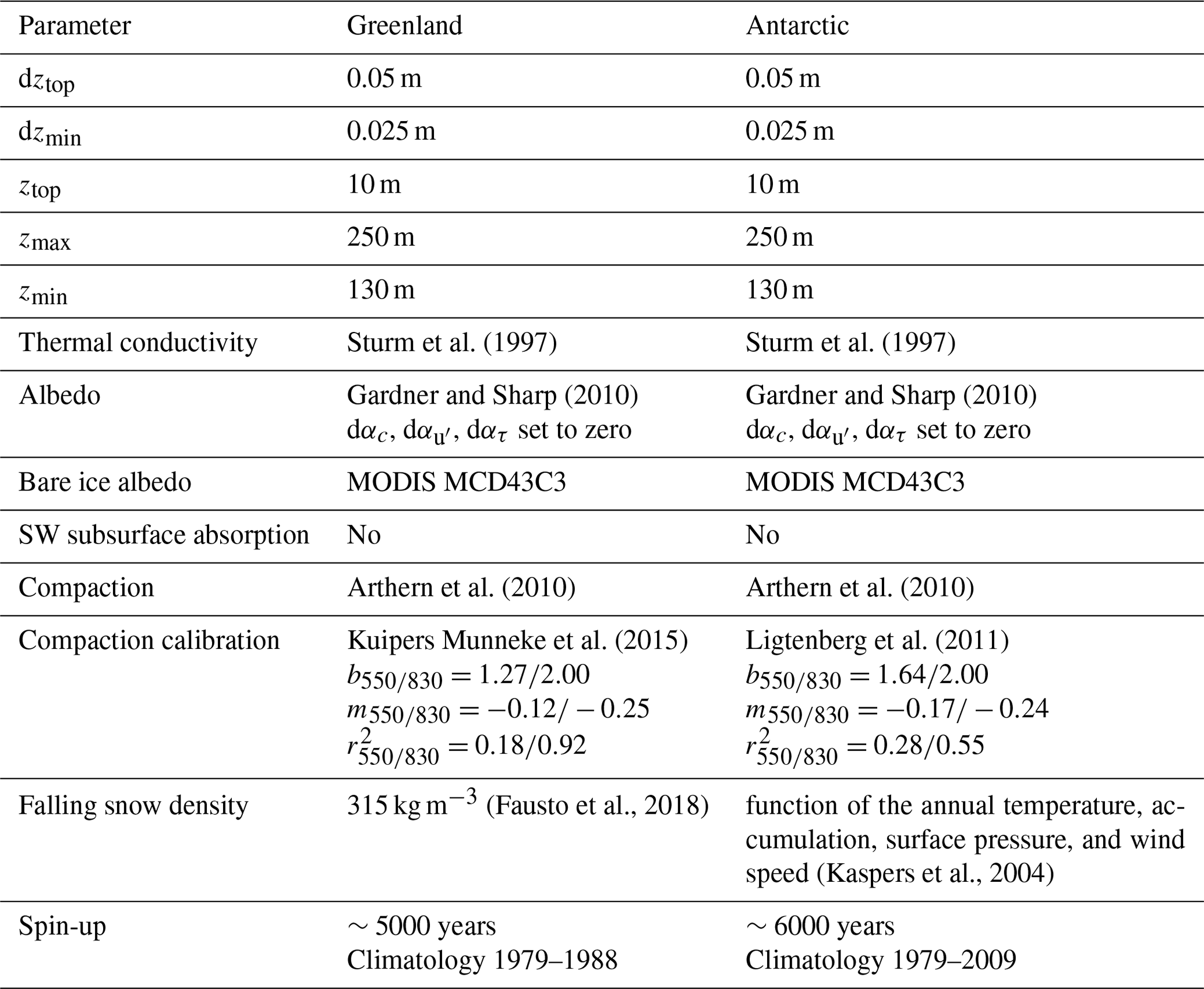
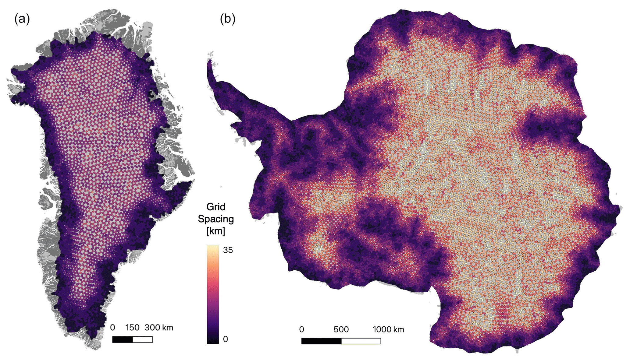
Figure 2 GEMB Greenland (a) and Antarctic (b) model node locations used for this study.

3 Study-specific model setup

3.1 Parameterization selection

GEMB v1.0 has many options for various model parameterizations. For this study we use a simplified version of the Gardner and Sharp (2010) albedo scheme in which albedo is modeled solely as a function of snow–ice grain specific surface area ($\widehat{S}$, surface area per unit mass). Subsurface shortwave penetration is turned off. Bare ice and shallow snow-covered ice albedo (areas with a surface density >820 kg m⁻³) are spatially varying and derived from the MODIS MCD43C3 16 d black-sky albedo product (Schaaf and Wang, 2015). Here, we determine the bare ice albedo by taking all summer (JJA) MCD43C3 16 d black-sky albedo values and calculating the lowest 10th percentile of measured albedos for every pixel. Bare ice albedos are not allowed to be less than 0.4. Albedos are then smoothed to a 0.25^∘ (∼32 km) resolution and bilinearly interpolated onto the GEMB model nodes. The smoothing is preformed to match the resolution of the ERA5 climate reanalysis data (Copernicus Climate Change Service, 2019), which is the forcing of choice when not comparing to the Institute for Marine and Atmospheric Research Utrecht Firn Densification Model (IMAU-FDM). The full list of selected model parameters used for this study is provided in Table 1.

3.2 Model grid

GEMB has no horizontal communication and thus easily supports nonuniform node spacing for computational efficiency; i.e., the model does not need to be run at the same spatial resolution as the climate forcing. This allows the model to use a coarser node spacing for areas with small spatial gradients in surface forcing (e.g., flat ice sheet interiors) and to use refined node spacing in areas of steep spatial gradients (e.g., areas of complex topography or near ice–ocean boundaries). For the Greenland simulations presented here, we use 10 990 nodes with node spacing ranging from 0.7 km along the coast to 21.1 km in the interior. For the Antarctic we simulate 50 390 nodes with node spacing ranging from 3.7 km along the periphery to 33.3 km in the interior. Node locations for both ice sheets are shown in Fig. 2.

3.3 Atmospheric forcing

For this study we force GEMB with climate data from the regional atmospheric climate model RACMO2.3p2 for the Antarctic (van Wessem et al., 2018) and RACMO2.3 for Greenland (Noël et al., 2016). Atmospheric fields of 10 m wind speed, 2 m temperature, surface pressure, incoming longwave and shortwave radiation, vapor pressure, and precipitation are supplied at 3 h resolution. The Antarctic product is provided at 27 km horizontal resolution for the years 1979 through 2014 and Greenland data at 11 km resolution for the years 1979 through 2014.

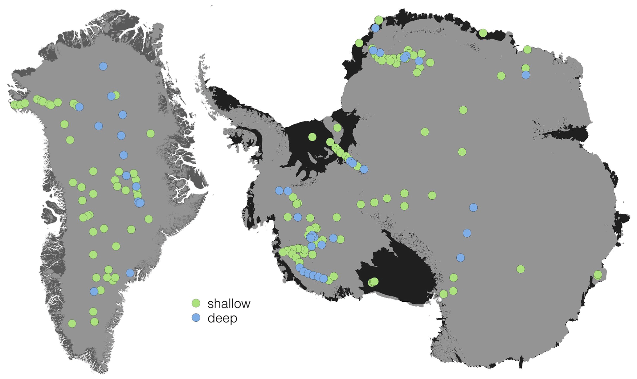
Figure 3 Locations of shallow (green) and deep (blue) firn cores. Firn cores are classified as shallow if they reach the 550 kg m⁻³ density horizon and deep if they extend to the 830 kg m⁻³ density horizon.

3.4 Firn model calibration

GEMB is run with the uncalibrated semi-empirical Arthern et al. (2010) firn model (Eq. 12) and is forced with a repeated cycle of historical climatology until a steady-state density profile is reached, e.g. 5000 years for Greenland and 6000 years for Antarctica. The depths of the modeled density horizons are extracted at the end of this spin-up procedure from the nodes that are closest in location to the firn cores used for calibration (Fig. 3). Here we use 64 shallow firn cores and 15 deep firn cores for calibration of Greenland firn and 117 shallow and 29 deep firn cores for calibration of Antarctic firn (Montgomery et al., 2018; Smith et al., 2020; Medley et al., 2022). Firn cores are classified as shallow if they reach beyond the 550 kg m⁻³ horizon up to the 830 kg m⁻³ horizon and deep if they reach beyond the 830 kg m⁻³ density horizon. Appendix A provides the full list of cores used in the calibration and validation along with the shallow or deep classification and citation.

For these firn core locations, MO₅₅₀ and MO₈₃₀ are plotted independently as functions of the natural log of $\dot{b}$ (see Eq. 16). A line is then fit through the points for each, representing the linear expression of how the model-to-observed depths vary as a function of $\dot{b}$ at each horizon. Next, the model steady-state spin-up is repeated, but this time multiplying the rate coefficients of c0 and c1 of the semi-empirical model of Arthern et al. (2010) (Eq. 12) by MO₅₅₀ and MO₈₃₀, respectively. Following Ligtenberg et al. (2011), MO₅₅₀ and MO₈₃₀ are allowed a minimum value of 0.25. Derived calibration offset ($b_{\mathrm{550}/\mathrm{830}}$) and scale ($m_{\mathrm{550}/\mathrm{830}}$) coefficients (Eq. 16) are provided in Table 1.

The new steady-state model density profiles are then verified against the calibration subset of firn cores as well as an additional withheld subset. Figure 4 shows the modeled vs. observed 550 and 830 kg m⁻³ depths for the uncalibrated and calibrated model runs.

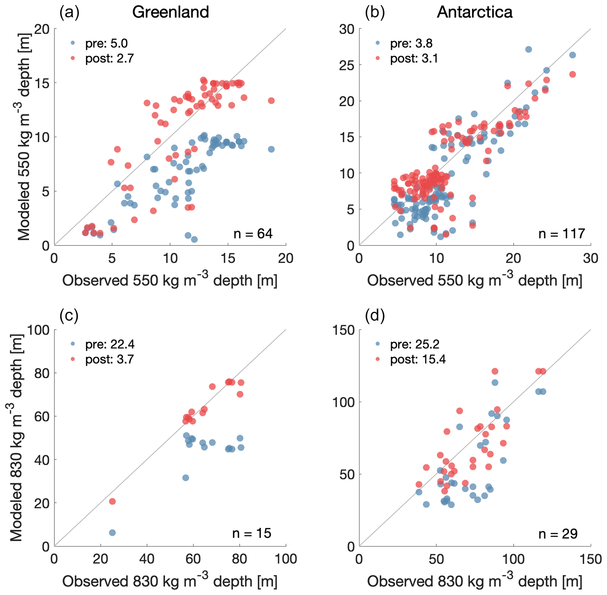
Figure 4 Comparison between modeled and observed 550 kg m⁻³ (a, b) and 830 kg m⁻³ (c, d) depths for the Greenland (a, c) and Antarctic (b, d) Ice Sheets for the locations of firn cores shown in Fig. 3. Blue markers show pre-calibrated model agreement with observations, and red markers show the post-calibrated model fit. The one-to-one line is shown by the black diagonal lines. Pre- and post-model calibration fits to observations (root mean square error: RMSE) are shown in the top left of each panel.

4 Comparison to other models

4.1 Surface mass balance

Here we compare the GEMB v1.0 surface mass balance (SMB) components to those computed within the RACMO surface model: RACMO2.3p2 for the Antarctic (van Wessem et al., 2018) and RACMO2.3 for Greenland (Noël et al., 2016). RACMO values are bilinearly interpolated to GEMB nodes. Since both GEMB and RACMO surfaces are forced with the same atmospheric data (RACMO), differences between modeled components can be directly attributed to differences in how surface processes are treated (e.g., albedo, roughness lengths, thermal diffusion). We also note that the RACMO surface model accounts for feedbacks between the atmosphere and the surface, while GEMB does not.

Figure 5 Mean 1979–2014 Greenland Ice Sheet GEMB (a, d, g) and RACMO (b, e, h) model output in meters of ice equivalent and their difference (c, f, i).

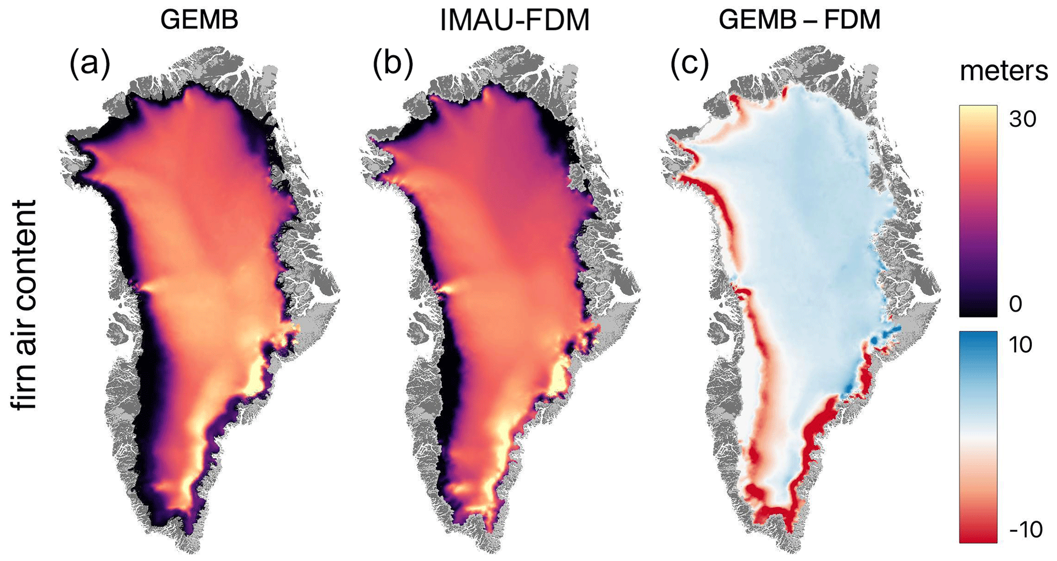
Figure 6 Mean 1979–2014 Greenland Ice Sheet GEMB (a) and IMAU-FDM (b) firn air content and their difference (c).

Figure 7 Mean 1979–2014 Antarctic Ice Sheet GEMB (left) and RACMO/IMAU-FDM (middle) model output in meters of ice equivalent and their difference (right). FDM is short for IMAU-FDM, the results of which are shown in the bottom row.

Mean spatial patterns of surface mass balance (i.e., accumulation (precipitation + deposition) − ablation (runoff + evaporation + sublimation)) and firn air content are shown for Greenland in Figs. 5 and 6, respectively, and for the Antarctic Ice Sheet in Fig. 7. The SMB patterns for the Antarctic Ice Sheet are driven largely by snowfall and sublimation, with little contribution from meltwater runoff. In Greenland, snowfall and runoff dominate. This largely explains the much closer agreement between models in the Antarctic vs. Greenland.

In Greenland the largest differences between models are concentrated in areas of high melt and low elevation that comprise the ice sheet periphery. In general, GEMB produces more negative surface mass balance in areas of maximum melt and slightly less negative surface mass balance near the equilibrium altitude. The more negative surface mass balance at lower elevations is most likely caused by a lower “bare ice” albedo in GEMB than in RACMO. Higher surface mass balance near the equilibrium line altitude is likely due to lower rates of fresh snowmelt. For the Antarctic, differences can largely be summarized as GEMB having higher rates of melt and runoff along the ice sheet periphery and lower rates of sublimation in areas conducive to katabatic winds (Parish and Bromwich, 1987). GEMB's higher rates of melt are most likely driven by lower surface albedo. Lower rates of sublimation can be attributed to the fact that GEMB does not yet (as of v1.0) include a model for snowdrift sublimation, while RACMO does (Lenaerts et al., 2010).

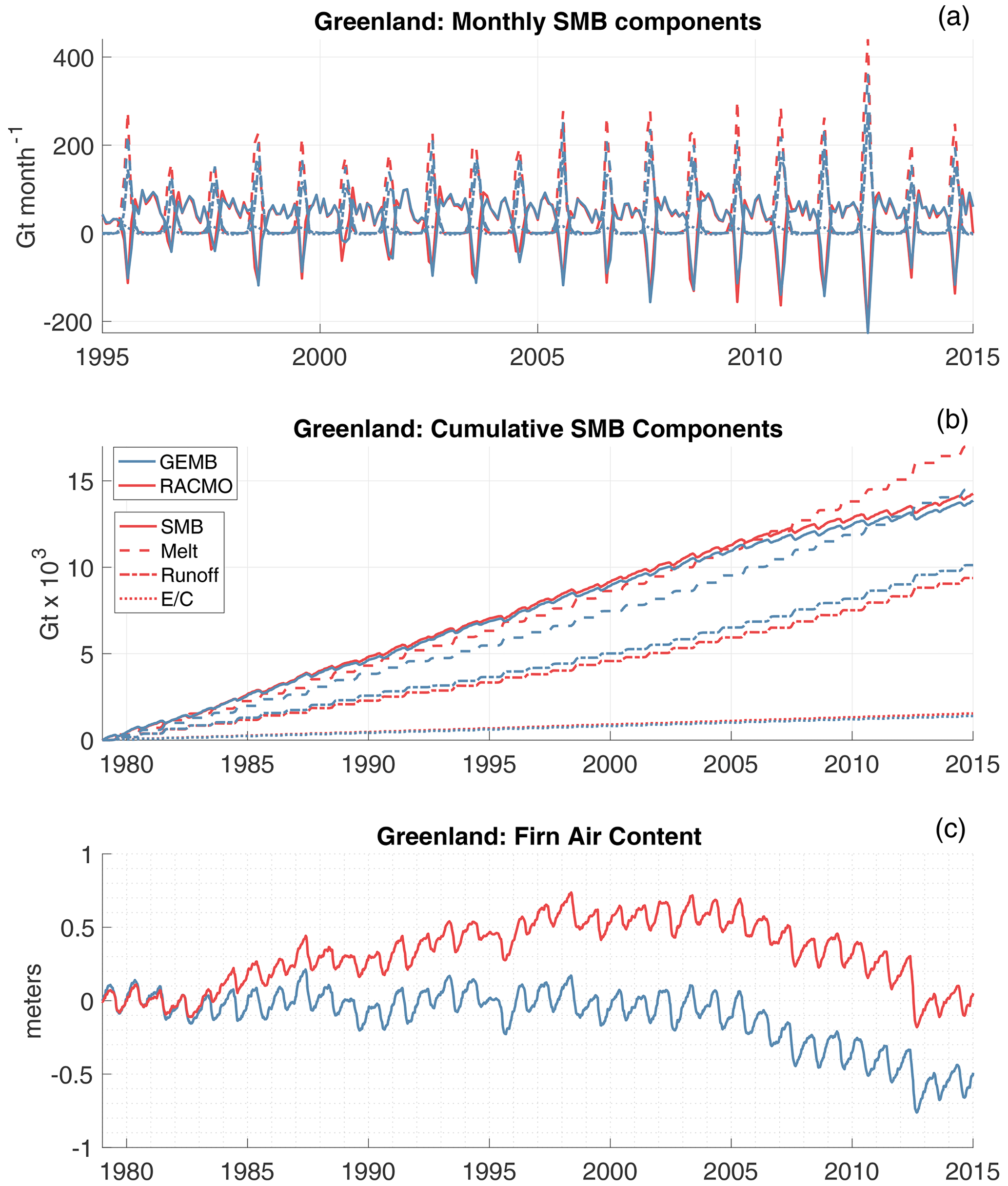
Figure 8 The 1979–2014 Greenland Ice Sheet GEMB (blue) and RACMO (red) monthly (a) and cumulative (b) model output. GEMB (blue) and IMAU-FDM (red) average fin air content anomaly, relative to 1979, is shown in panel (c). $E/C$ is the mass change due to evaporation, condensation, sublimation, and deposition.

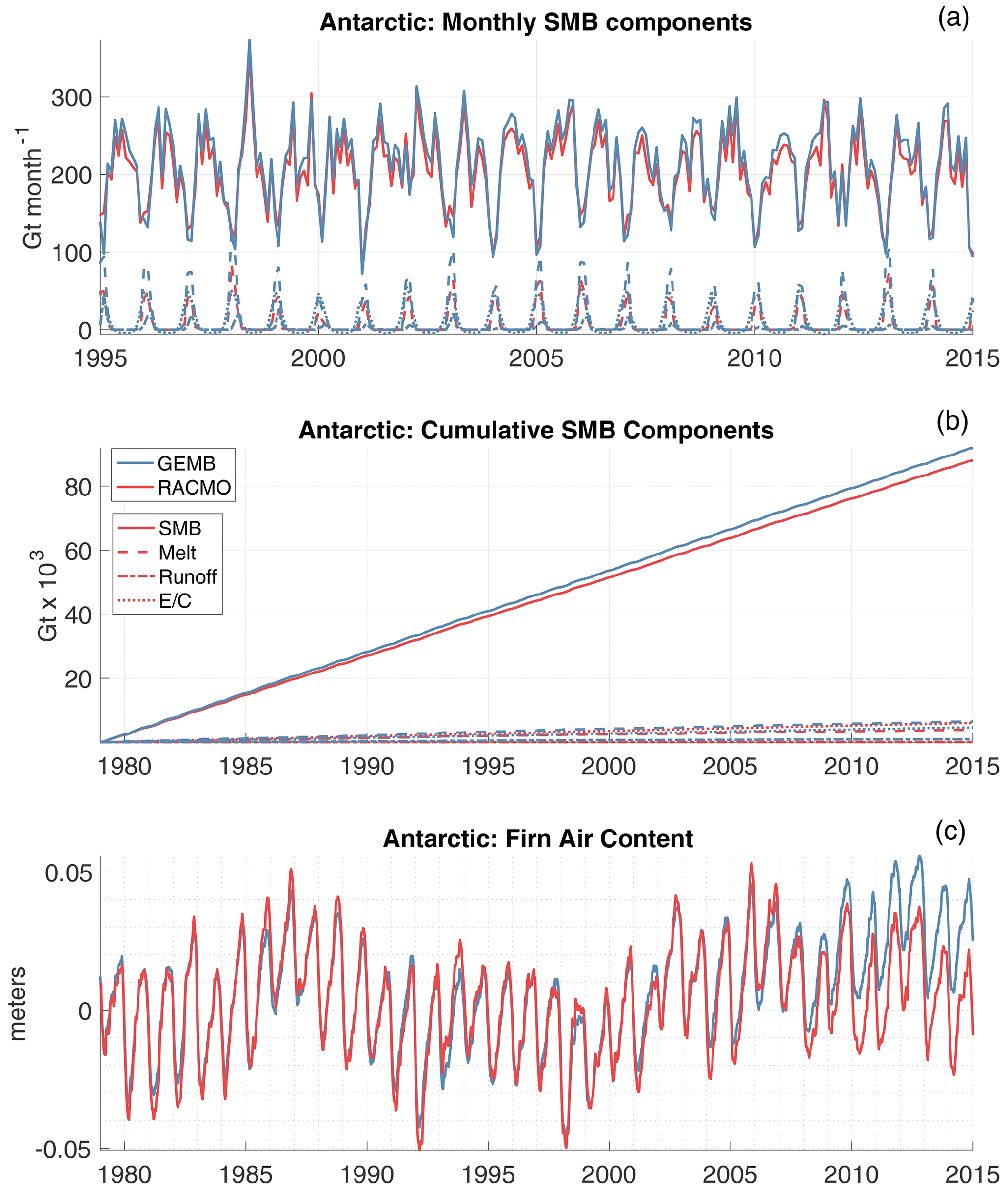
Figure 9 The 1979–2014 Antarctic Ice Sheet GEMB (blue) and RACMO (red) monthly (a) and cumulative (b) model output. GEMB (blue) and IMAU-FDM (red) average fin air content anomaly, relative to 1979, is shown in panel (c). $E/C$ is the mass change due to evaporation, condensation, sublimation, and deposition.

Looking at Greenland (Fig. 8) and Antarctic (Fig. 9) monthly (a) and cumulative (b) time series of surface mass balance components we find very close agreement between GEMB and RACMO. Agreement is so close that several RACMO variables are not visible in the monthly time series (Figs. 8a and 9a) as they are overlaid by nearly identical GEMB output. The most notable difference is higher rates of melt for RACMO simulations in Greenland that are largely compensated for by increased meltwater retention within the firn. In the Antarctic lower rates of sublimation and higher rates of meltwater runoff in GEMB result in a slightly more positive surface mass balance trend relative to those simulated by RACMO.

4.2 Firn air content

Next, we compare firn properties as modeled by GEMB v1.0 to those modeled by IMAU-FDM (Ligtenberg et al., 2011) for Greenland (Ligtenberg et al., 2018) and the Antarctic (Ligtenberg et al., 2011) forced with the same RACMO data as used by the GEMB simulations (see the “Study-specific model setup” section and Table 1). Like GEMB, IMAU-FDM is an uncoupled firn model (i.e., not coupled with the atmospheric model). IMAU-FDM is a widely used firn model product. We note that there has been a recent and rapid increase in the number of ice-sheet-wide firn modeling studies (Brils et al., 2022; Dunmire et al., 2021; Keenan et al., 2021; Medley et al., 2022; Veldhuijsen et al., 2022). An in-depth comparison between all modeled results would be highly valuable but is not done here. We first look at the spatial patterns of total firn air content (FAC), which is the depth of air in meters per unit area. For Greenland, GEMB tends to generate lower FAC relative to IMAU-FDM in the west and southeast percolation zones along the ice sheet margins and a slightly higher FAC in the northeast (Fig. 6). This is counterintuitive as GEMB is shown to produce less melt than RACMO in areas where RACMO has a higher FAC; we would expect the opposite to be true. This difference is likely the result of a slightly more aggressive compaction calibration scaling coefficient used by GEMB (Table 1: $b_{\mathrm{550}/\mathrm{830}}=\mathrm{1.27}/\mathrm{2.00}$, $m_{\mathrm{550}/\mathrm{830}}=-\mathrm{0.12}/-\mathrm{0.25}$) relative to those used by IMAU-FDM ($b_{\mathrm{550}/\mathrm{830}}=\mathrm{1.04}/\mathrm{1.73}$, $m_{\mathrm{550}/\mathrm{830}}=-\mathrm{0.09}/-\mathrm{0.20}$). Differences in calibration coefficients can be attributed to differences in the firn cores used for the calibration, as IMAU-FDM had access to fewer cores when calibrated, and differences in the firn models themselves.

In the Antarctic there is generally better agreement between models and scaling coefficients of $b_{\mathrm{550}/\mathrm{830}}=\mathrm{1.64}/\mathrm{2.00}$ and $m_{\mathrm{550}/\mathrm{830}}=-\mathrm{0.17}/-\mathrm{0.24}$ for GEMB and $b_{\mathrm{550}/\mathrm{830}}=\mathrm{1.44}/\mathrm{2.37}$ and $m_{\mathrm{550}/\mathrm{830}}=-\mathrm{0.15}/-\mathrm{0.29}$ for IMAU-FDM (Kuipers Munneke et al., 2015). Differences between GEMB and IMAU-FDM can be characterized as GEMB having lower FAC at low elevations and slightly higher FAC at higher elevations (Fig. 7). This pattern can be attributed to GEMB having warmer surface temperatures (higher melt) at lower elevations and a smaller b₈₃₀ scaling coefficient that will impact total FAC most in areas with deep firn (i.e., the Antarctic Plateau).

It should be noted that for the runs presented here GEMB assumes an incompressible ice density of 910 kg m⁻³, while IMAU-FDM uses 917 kg m⁻³. The overall impact of this assumption, when comparing total FAC between models, will at worst be a 0.76 % underestimate by GEMB for those columns that do not densify to ice by the time they reach the bottom of the model domain (i.e., Antarctic interior) relative to IMAU-FDM. For all other locations the difference will be significantly less.

Looking at the temporal evolution in FAC for both Greenland (Fig. 8) and Antarctica (Fig. 9) it can be seen that seasonal fluctuations and interannual variations are in very close agreement for both ice sheets, but deviations in long-term trends are apparent. For the model runs examined GEMB is spun up using the 1979–1988 climatology repeated for 5000 years for Greenland and the 1979–2009 climatology repeated for 6000 years for Antarctica. IMAU-FDM is spun up using the 1960–1979 climatology repeated for as many years as it takes for the mean annual accumulation rate multiplied by the spin-up length to equal the thickness of the firn layer (from the surface to the depth at which the ice density is reached: Kuipers Munneke et al., 2015).

For Greenland (Fig. 8c) GEMB has virtually no trend in FAC between 1979 and 2005, becoming more negative thereafter coincident with increases in summer melt. IMAU-FDM FAC trends positive between 1979 and 2005 after which the trend becomes negative, closely matching the rate of FAC loss simulated by GEMB. Differences in FAC trend between 1979 and 2005 can be attributed to differences in model spin-up that are known to be a major source of uncertainty in FAC trends (Kuipers Munneke et al., 2015). Since GEMB is spun up using the 1979–1988 climatology, there should be little trend in FAC over this period. GEMB was initialized to the 1979–1988 climatology as the 1960–1979 period was not included with the provided RACMO forcing. In addition, climate reanalyses are known to perform considerably better after the introduction of satellite data in 1978. This is especially true over the poles where in situ observations are sparse (Tennant, 2004). The difference in prescribed spin-up climatology between the two models is the most likely cause of the observed differences in FAC trend between 1979 and 2005. When the 1979–2005 FAC trend is removed from both products (not shown), the FAC time series are nearly identical until 2004 after which GEMB estimates ∼0.5 m of FAC loss and IMAU-FDM estimates ∼1.0 m of FAC loss between 2004 and 2015. Some of the difference in trend can be attributed to IMAU-FDM having higher rates of melt along the equilibrium altitude during this period of time (Fig. 5).

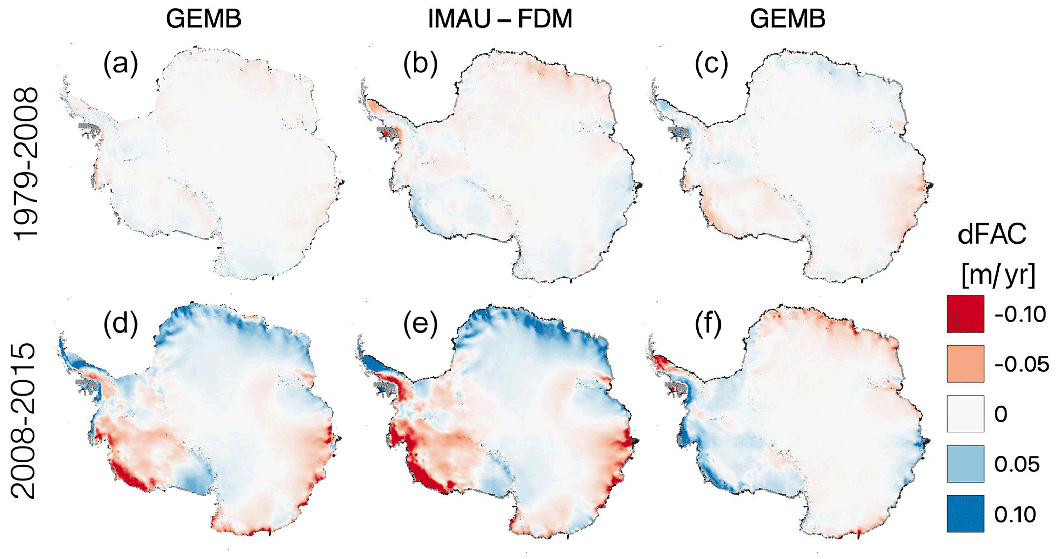
Figure 10 Rate of firn air content change (dFAC) for the Antarctic Ice Sheet as modeled by GEMB (a, d) and IMAU-FDM (b, e), as well as their difference (c, f). Rates for the period 1979–2008 are shown in panels (a)–(c), and rates for the 2008–2015 period are shown in panels (d)–(f).

Changes in FAC for the Antarctic (Fig. 9c) are nearly identical between models with a notable divergence beginning in 2008, after which GEMB FAC trends slightly positive and IMAU-FDM FAC trends slightly negative. Spatial patterns of FAC trends for the period pre- and post-2008 (Fig. 10) show much larger rates of FAC change for the 2008–2015 period with IMAU-FDM tending to have the same sign but larger trends than GEMB. For the post-2008 period, GEMB FAC gains outcompete losses, resulting in a slight positive trend in FAC over this period that is not seen in IMAU-FDM.

Despite a desire to identify which model is closer to the truth, we do not yet have an objective way to determine that. Likely the most definitive analysis will be to compare FAC-corrected altimetry (e.g., ICESat/2) estimates of ice sheet mass change to mass changes derived from satellite gravimetry (i.e., GRACE/FO) data, but that is beyond the scope of this study.

5 Model sensitivity to vertical resolution

Firn and surface mass balance models are highly sensitive to the chosen setup and empirical parameterizations (Bougamont et al., 2007; Kuipers Munneke et al., 2015). Major sources of uncertainty include parameterizations of albedo, snow grain growth, surface roughness, densification and its calibration (Stevens et al., 2020), and thermal conductivity. These uncertainties become exacerbated with the introduction of liquid water into the firn column (Vandecrux et al., 2020). Model setup can also introduce large sources of uncertainty and error. Three particularly important decisions are the choice of spin-up climatology (Kuipers Munneke et al., 2015), the length of time the spin-up is run (needs to reach equilibrium to prevent model drift), and the vertical resolution of the model. Most of these sensitivities have been explored extensively, and we direct the reader to previous publications that explore these topics in detail (e.g., Bougamont et al., 2007; Kuipers Munneke et al., 2015; Vandecrux et al., 2020; Stevens et al., 2020; Lundin et al., 2017).

One model sensitivity that we have not seen covered elsewhere is the sensitivity of the model to the vertical resolution of the firn column. The vertical resolution can have a large impact on melt rates and surface temperatures. This is because all of the energy and mass transfer between the atmosphere and the surface are often allocated to the model's uppermost layer in the firn column. A thicker layer will tend to dampen fluctuations in thermal energy relative to a thinner layer. Since snow grain growth, snow–ice melt, and compaction have nonlinear relations to temperature, model results will diverge for differing vertical resolutions. This is most true for the near-surface layers as thermal gradients are attenuated with depth.

Figure 11 GEMB change in the modeled rate of melt (a–c) as well as evaporation and condensation (d–f) for near-surface model layer depths (dz_top) of 5, 10, and 20 cm relative to a near-surface model layer depth of 2 cm.

To demonstrate model sensitivity to vertical resolution we run GEMB v1.0 for Greenland using the same model setup (Table 1) but for four different dz_top [2, 5, 10, 20 cm] and dz_min [1, 2.5, 5, 10 cm] pairs (i.e., four model runs each having $\mathrm{d}{z}_{\min }=\mathrm{1}/\mathrm{2}\mathrm{d}{z}_{\mathrm{top}}$). Results of the simulations are shown in Fig. 11. Increasing the size of the top layers results in a progressive reduction in melt as diurnal peak temperatures are muted and vertical gradients in temperature are reduced, in turn reducing grain metamorphism and surface darkening. Increasing the size of the top layers also results in stronger thermal gradients between the atmosphere and the surface that drive larger (both positive and negative) surface latent and sensible heat and mass fluxes. This has more impact in summer when diurnal fluctuations are larger than during polar night when diurnal changes in temperature are small or nonexistent. The net effect of increasing the surface layer thickness is slightly lower evaporation and sublimation losses.

6 Comparison of modeled and observed near-surface temperatures

To demonstrate the model's skill at simulating near-surface temperature, we compare GEMB v1.0 model output to an observational dataset of near-surface firn temperature that was collected at Summit Station, Greenland (Miller et al., 2017). Here, subsurface temperatures are measured using thermistors buried within the snowpack every 20 cm from July 2013 to June 2014. We compare these observations against results produced by GEMB v1.0 forced with RACMO output (see Table 1), rerun to output concurrent daily model solutions for the location of the observations (72.580^∘ N, 38.459^∘ W). We correct the data for change in thermistor depth over time. By default, GEMB's thermal conductivity is calculated as a function of snow density, after Sturm et al. (1997). To investigate model sensitivity to thermal conductivity, we also run the same simulation using the density-dependent thermal conductivity relation suggested by Calonne et al. (2011, Eq. 12). As demonstrated by Calonne et al. (2011), their solution gives a higher thermal conductivity for an equivalent density, which sits just inside the upper bounds of the 95 % confidence interval reported by Sturm et al. (1997). Here we compare results between the two GEMB simulations and the observations. For simplicity, all results are plotted with respect to the modeled or observed surface. Note that since the first thermal probe was placed at a depth of 20 cm below the surface, observational values between the snow surface and 20 cm depth are extrapolations.

Figure 12 Observed and modeled daily near-surface (upper 2 m) temperatures for Summit Station, Greenland (72.580^∘ N and 38.459^∘ W), from July 2013 to June 2014. Temperature profiles from (a) observations (Miller et al., 2017), (c) modeled using GEMB and Sturm et al. (1997) thermal conductivity, and (e) modeled using GEMB and Calonne et al. (2011) thermal conductivity. (b) Observed downward shortwave (dsw) and longwave (dlw) radiation provided for context. Differences between temperature profiles for (d) GEMB–Sturm and observations and for (f) GEMB–Calonne and observations. Note: all GEMB simulations are forced with RACMO model output (see Table 1), and therefore modeled temperature differences relative to observations are due to errors in forcing, model parameterizations, and observations.

Figure 12a, c, and e show the thermal profiles to a depth of 2 m for observed, GEMB–Sturm, and GEMB–Calonne temperatures, respectively. Figure 12b shows the observed radiative fluxes, and Fig. 12d and f show the difference between modeled and observed snow temperature profiles. Overall, there is very good agreement between the modeled and observed thermal profiles with differences resulting from errors in atmospheric forcing, errors in observations, and biases attributed to errors in model parameterizations. Both model simulations produce mean temperatures between 0.2 and 2 m depth that are ∼0.8 K warmer than the observations, with the Sturm parameterization of thermal conductivity producing slightly better agreement (0.77 K) than the Calonne parameterization (0.79 K). Looking at bias and root mean square error as a function of depth, it can be seen (Fig. 13) that the Sturm parameterization produces slightly better agreement with the observations in the top 0.5 m of the snowpack, while the Calonne parameterization produces a significantly better fit for depths below 0.8 m. From this single location comparison, the Calonne parameterization outperforms the Sturm parameterization. Drawing any more definitive conclusions is challenging given other sources of disagreement such as atmospheric forcing and density structure.

Figure 13 Mean bias (left) and RMSE (right) in modeled near-surface temperatures as a function of depth relative to observations (Miller et al., 2017). Daily GEMB model results using Sturm et al. (1997) and Calonne et al. (2011) thermal conductivity parameterizations for Summit Station, Greenland (72.580^∘ N and 38.459^∘ W), from July 2013 to June 2014.

While differences in mean temperature are only ∼0.8 K, seasonal differences can be as large as 5 K (Fig. 13). A 5 K increase in snow–firn temperature increases the compaction rate by a factor of 1.6–1.8. Since compaction rates are strongly dependent on temperature, seasonal biases in temperate have a large impact on rates of firn compaction, even if annual biases are small. Therefore, future work should prioritize improving near-surface atmospheric temperatures over glacier surfaces, from both models and observations, and thermal diffusion within snow and ice.

Calonne et al. (2019) show that the quadric relations between effective thermal conductivity and density, which are often used for snow (e.g., Eqs. 4 and 5), do not perform well for firn and porous ice. Instead, they propose an alternative empirical relation to more accurately model effective conductivity for the full range of densities from 0 to 917 kg m⁻³ (see Eq. 5 in Calonne et al., 2019). We plan to include empirical relations proposed by Calonne et al. (2019) in a future version of GEMB.

7 Summary and conclusions

This paper provides the first description of the open-source Glacier Energy and Mass Balance (GEMB) model that has been integrated as a module into the Ice-sheet and Sea-level System Model (ISSM). The model is one-way coupled with the atmosphere, which allows it to be run offline with a diversity of climate forcing but neglects feedback to the atmosphere. GEMB is written in C++, which produces efficient compiled machine code for fast execution. GEMB provides numerous parameterization choices for various key processes (e.g., albedo, subsurface shortwave absorption, and compaction), making it well suited for uncertainty quantification and model exploration.

To evaluate output from GEMB we compare it to the model output from the Institute for Marine and Atmospheric Research Utrecht Firn Densification Model (IMAU-FDM: Ligtenberg et al., 2011) for both Greenland (Ligtenberg et al., 2018) and the Antarctic (Ligtenberg et al., 2011). Models are forced with the same RACMO climate data (see the “Study-specific model setup” section, Table 1) and are independently calibrated to ice core density profiles. By forcing GEMB with the same climate data as IMAU-FDM we are able to attribute differences in model output to differences in model parameterizations and setup.

Overall, we find good agreement between models for both ice sheets with a few notable differences. For Greenland GEMB produces considerably less melt than IMAU-FDM but nearly as much runoff. This is because, relative to IMAU-FDM, GEMB tends to generate more low-elevation melt that runs off and less high-elevation melt that refreezes within the firn. These differences are most likely due to inter-model differences in the bare ice albedo and fresh snowmelt. GEMB and IMAU-FDM produce considerably different trends in FAC that are the result of differing climatologies used for model spin-up. GEMB used the 1979–1988 climatology repeated for 5000 years, while IMAU-FDM used the 1960–1979 climatology. This results in GEMB having little trend in FAC prior to the onset of increased melting in 2005. In contrast, IMAU-FDM has a positive FAC trend from 1979–2005 and a negative trend thereafter. These differences can have a large impact on volume-to-mass conversions used to generate glacier mass change estimates from satellite altimetry. For the Antarctic, GEMB and IMAU-IMAU-FDM are nearly identical with GEMB having slightly lower rates of sublimation and slightly higher rates of meltwater runoff that lead to a slightly more positive surface mass balance trend than found in IMAU-FDM. Changes in FAC for the Antarctic are nearly identical between models with a notable divergence beginning in 2008, after which GEMB FAC trends slightly positive and IMAU-FDM FAC trends slightly negative.

To demonstrate the impact of model setup we explore the impact of the model's vertical resolution on the results. We show that coarsening the model's vertical resolution decreases melt and increases surface latent and sensible heat fluxes due to stronger thermal gradients between the surface and the atmosphere. Lastly, we compare modeled near-surface thermal profiles, calculated using two different density–thermal conductivity relations, to in situ observations collected at Summit Station, Greenland. Our comparison shows good agreement between modeled and observed temperatures, with slightly improved agreement using the Calonne versus the Sturm thermal conductivity parameterization.

Our analysis shows that the GEMB model performs as expected and produces results that are comparable to an existing state-of-the-art firn model (IMAU-FDM). There are notable differences in output between the models, but it is difficult to judge if one model outperforms the other as there are insufficient observational data to distinguish between models. Future studies that compare altimetry-derived mass changes with those derived from satellite gravimetry should help to distinguish between models.

Future work will focus on developing atmospheric and firn downscaling routines that will allow GEMB to produce higher-resolution output when forced with medium-resolution (30–100 km) climate reanalysis or coarse-resolution (200–500 km) climate model output.

Appendix A

Table A1 The following tables list the cores, taken from Montgomery et al. (2018) and Medley et al. (2022), and their citations. Those used for deep core calibration analysis (density of 830 kg m⁻³) and shallow core calibration analysis (density of 550 kg m⁻³) are marked in the corresponding “Deep” and “Shallow” columns. Cores without a deep or shallow designation were used for model evaluation.