the Creative Commons Attribution 4.0 License.
the Creative Commons Attribution 4.0 License.
 | 22 Mar 2023
Continental-scale evaluation of a fully distributed coupled land surface and groundwater model, ParFlow-CLM (v3.6.0), over Europe
Wendy Sharples
Yueling Ma
Klaus Goergen
Stefan Kollet
High-resolution large-scale predictions of hydrologic states and fluxes are important for many multi-scale applications, including water resource management. However, many of the existing global- to continental-scale hydrological models are applied at coarse resolution and neglect more complex processes such as lateral surface and groundwater flow, thereby not capturing smaller-scale hydrologic processes. Applications of high-resolution and physically based integrated hydrological models are often limited to watershed scales, neglecting the mesoscale climate effects on the water cycle. We implemented an integrated, physically based coupled land surface groundwater model, ParFlow-CLM version 3.6.0, over a pan-European model domain at 0.0275∘ (∼3 km) resolution. The model simulates a three-dimensional variably saturated groundwater-flow-solving Richards equation and overland flow with a two-dimensional kinematic wave approximation, which is fully integrated with land surface exchange processes. A comprehensive evaluation of multiple hydrologic variables including discharge, surface soil moisture (SM), evapotranspiration (ET), snow water equivalent (SWE), total water storage (TWS), and water table depth (WTD) resulting from a 10-year (1997–2006) model simulation was performed using in situ and remote sensing (RS) observations. Overall, the uncalibrated ParFlow-CLM model showed good agreement in simulating river discharge for 176 gauging stations across Europe (average Spearman's rank correlation (R) of 0.77). At the local scale, ParFlow-CLM model performed well for ET (R>0.94) against eddy covariance observations but showed relatively large differences for SM and WTD (median R values of 0.7 and 0.50, respectively) when compared with soil moisture networks and groundwater-monitoring-well data. However, model performance varied between hydroclimate regions, with the best agreement to RS datasets being shown in semi-arid and arid regions for most variables. Conversely, the largest differences between modeled and RS datasets (e.g., for SM, SWE, and TWS) are shown in humid and cold regions. Our findings highlight the importance of including multiple variables using both local-scale and large-scale RS datasets in model evaluations for a better understanding of physically based fully distributed hydrologic model performance and uncertainties in water and energy fluxes over continental scales and across different hydroclimate regions. The large-scale, high-resolution setup also forms a basis for future studies and provides an evaluation reference for climate change impact projections and a climatology for hydrological forecasting considering the effects of lateral surface and groundwater flows.
- Article
(10660 KB) - Full-text XML
-
Supplement
(6145 KB) - BibTeX
- EndNote


Continental-scale, high-resolution (<5 km) hydrologic modeling is important to understand and predict water cycle changes over large scales (Döll et al., 2003) and the spatial distribution of land–atmosphere moisture and energy fluxes (Maxwell et al., 2015), including their spatiotemporal variability (Schwingshackl et al., 2017). Predicting changes in water cycle processes over larger scales is also necessary to capture macro-scale processes which can affect water security. Such processes, for example, include high evapotranspiration rates, which lead to soil moisture or water storage deficits and result in mega droughts over large areas (for example, the 2018 to 2020 European drought; Rakovec et al., 2022; Hanel et al., 2018), or an increase in heavy rainfall events caused by climate change, resulting in soil moisture surpluses and widespread flooding (e.g., western European floods in 2021; He et al., 2022). In addition, it is important to accurately model interactions between surface and groundwater processes, as they can affect large-scale climatological and hydrological patterns (Fan, 2015) and exert a major control on river ecosystems at local to regional scales (Ji et al., 2017).
Numerical models that attempt to simulate large-scale hydrology and associated processes are usually categorized as land surface models (LSMs) or global hydrological models (GHMs). These models have been developed for simulating the land surface water, energy and momentum exchange (Sellers et al., 1988) to provide water balance estimates at a global to continental scale (e.g., Döll et al., 2003; Hunger and Döll, 2008; Gudmundsson et al., 2012; Haddeland et al., 2011). Despite the extensive work in large-scale hydrology modeling (e.g., Clark et al., 2015), many of the existing large-scale hydrological models (both LSMs and GHMs), especially those intended for continental- to global-scale simulations, are single-column models for which most hydrological processes are implemented empirically and at a coarse spatial resolution (typically 25 to 100 km). As a result, many of the important hydrological processes are simplified, including groundwater and surface water dynamics, soil moisture re-distribution, and evapotranspiration (Clark et al., 2017). In most large-scale continental or global models, the representation of the groundwater dynamics is either not included or oversimplified, which may lead to errors in the prediction of hydrologic states and fluxes (Martínez-de la Torre and Miguez-Macho, 2019) or an underestimation of total water storage trends (Scanlon et al., 2018). A physics-based integrated hydrological model, on the other hand, which can simultaneously solve surface and subsurface systems with lateral groundwater flow, may provide better predictions of both local and global water resources (Beven and Cloke, 2012). Many recent studies have shown the importance of representing the 3-D groundwater component in GHMs (e.g., PCR-GlobWB and WaterGAP (G3M); Verkaik et al., 2022; Reinecke et al., 2019) and/or lateral transport of subsurface water and its interaction with land–atmosphere water fluxes (e.g., Barlage et al., 2021; Keune et al., 2016; Maxwell and Kollet, 2008; Miguez-Macho and Fan, 2012; Miguez-Macho et al., 2007; Xie et al., 2012; Zeng et al., 2018). These studies suggested that explicitly simulating these processes can have a significant effect on the accuracy of surface energy fluxes (Keune et al., 2016) and flux partitioning (Maxwell and Condon, 2016). It can also affect the accuracy of the spatial redistribution of soil moisture through infiltration during lateral movement of water (Ji et al., 2017). Furthermore, processes-based integrated hydrologic models can better characterize spatial heterogeneity in water and energy states and fluxes when run at a high spatial resolution (<5 km) due to the higher-resolved surface properties, providing a more accurate representation of the lateral transports of surface and subsurface water movements driven by topographic slopes (Ji et al., 2017; Shrestha et al., 2014; Barlage et al., 2021). However, the effect of these important processes on water and energy states and fluxes is still not fully understood, especially over continental scales, and a more comprehensive assessment of model performance across different hydroclimates and hydrological characteristics is needed.
In the past decade, there has been a growing interest in developing and implementing hyperresolution hydrological modeling over large domains with more realistic representation of surface and subsurface lateral flow and groundwater dynamics (e.g., Lawrence et al., 2019; Pokhrel et al., 2021; Zeng et al., 2018; Grimaldi et al., 2019). It is challenging to implement and evaluate fully distributed integrated surface and groundwater models over large spatial domains, particularly given the lack of consistent large-scale hydrogeological information (de Graaf et al., 2020) and/or the computational cost to implement such models over larger domains. With the advancement of computing resources and the availability of gridded datasets at a global scale, e.g., soil (Hengl et al., 2017, SoilGrids) and hydrogeological parameters (Gleeson et al., 2014; de Graaf et al., 2020), a handful of modeling studies have fully utilized parallel-computing systems to explicitly simulate the three-dimensional spatial dynamics of water fluxes and state variables at higher resolutions (12 to 1 km) over regional and continental scales (e.g., Keune et al., 2016, 2019; Kollet et al., 2018; Tijerina et al., 2021; O'Neill et al., 2021). Fully integrated models used in these studies are often not calibrated, mainly due to the computational cost to simultaneously solve surface and groundwater equations and the presence of nonlinear dependencies between different subsystems, which makes the parameter calibration more difficult (Hill and Tiedeman, 2006). For such models, finding global optimum solutions may require efficient nonlinear optimization techniques to perform multivariate, multi-objective calibration (e.g., Tolley et al., 2019; Rafiei et al., 2022). Therefore, a comprehensive evaluation of the performance of uncalibrated large-scale fully integrated models with available in situ and remotely sensed observations for water balance components serves as an assessment of the model uncertainty. Simulation performance benchmarks can be set and met before application of the model in forecast or projection studies.
Many of the continental- to global-scale modeling studies solely evaluate streamflow performance of the models, mostly for large rivers (e.g., Haddeland et al., 2011; Zhou et al., 2012; Gudmundsson et al., 2012). While these studies showed robust skill in terms of overall streamflow dynamics for a range of watershed sizes, little consideration has been given to other components for water balance closure and characterization of hydrologic states, e.g., soil moisture and groundwater levels. Bouaziz et al. (2021) examined multiple states and flux variables from 12 hydrological models. They showed similar streamflow performance but identified substantial dissimilarities in snow water storage, root zone soil moisture (SM) and total water storage when compared with observations. These results suggest that, while most models show similar performance in simulating streamflow, they may not realistically simulate other components of the water balance. Therefore, it is important to assess the model performance not only for streamflow but for other hydrologic states and fluxes with available observations such as SM, evapotranspiration (ET), water table depth (WTD), snow water equivalent (SWE), and total water storage (TWS), especially for spatially distributed models which are able to simulate full hydrologic heterogeneity. Furthermore, using additional variables for an evaluation of fully distributed models with explicit groundwater lateral-flow representation is also important to identify uncertainties in surface and groundwater interactions (e.g., O'Neill et al., 2021) and mismatches between the spatiotemporal representation of hydrologic fluxes and states (e.g., Rakovec et al., 2016).
In this study, we implement the ParFlow-CLM model (Kollet and Maxwell, 2008; Kuffour et al., 2020), which is a physically based integrated hydrological model that simultaneously solves surface and subsurface processes with lateral groundwater flow and assess its performance for multiple variables, hydroclimates and hydrological characteristics over a pan-European domain. We undertake this thorough assessment in order to perform a holistic model evaluation for the aforementioned reasons. Building on previous studies, we follow a similar approach to O'Neill et al. (2021) to assess our model performance over a pan-European domain at 3 km resolution. To the best of our knowledge, this is the first study to implement ParFlow-CLM over the pan-European domain at a high resolution (0.0275∘ (∼3 km)) with lateral surface and groundwater flow representation over a timescale large enough to consider climate variability (10 years). Previously, the ParFlow-CLM model has been employed over the pan-European domain at 12 km resolution for the year 2003 within the framework of a fully integrated soil–vegetation–atmosphere model (e.g., Keune et al., 2016, 2019; Furusho-Percot et al., 2019; Hartick et al., 2021). However, the model performance was not rigorously evaluated for all water balance components, given the coarser resolution and the focus on atmosphere–land surface–groundwater feedback. Similarly, ParFlow-CLM has been implemented over the continental US (CONUS) at a 1 km resolution (Maxwell et al., 2015; Condon and Maxwell, 2015, 2017; Maxwell and Condon, 2016), where most recently, O'Neill et al. (2021) provided a comprehensive multi-variable evaluation of CONUS implementation across a simulation time period of 4 years. They highlighted the importance of evaluating the continental-scale water balance as a whole for a process-based understanding of model performance and bias. In this study, implementation of the ParFlow-CLM model outside CONUS is also a step forward towards “Hyperresolution global land surface modeling” which is considered a “grand challenge in hydrology”, as described by Wood et al. (2011), Bierkens et al. (2015) and Condon et al. (2021).
Here, we focus on the application and performance of ParFlow-CLM for a 3 km resolution pan-European model domain and perform simulations over a period of 10 years (1997–2006). For comprehensive model evaluation, we present a comparison of model results with various in situ and several remote sensing (RS) products and assess model performances for multiple hydrologic variables such as surface SM, river discharge, ET, SWE, WTD, and TWS for different hydroclimate regions. Comparisons with a variety of in situ and satellite-based gridded RS products allows us to evaluate model performance not only at grid cell scale but also at large spatial scales to better understand both seasonal and spatial variability for different regions influenced by different climatic conditions. In addition, to discuss how our model differs from other existing implementations of ParFlow-CLM, we compare our results with the CONUS implementation of ParFlow-CLM model (O'Neill et al., 2021) to highlight model strengths and weaknesses in simulating continental-scale water balance components. This evaluation can serve as a benchmark and baseline for future ParFlow-CLM implementations over Europe and could be used as an evaluation framework for future model development.
In Sect. 2, we describe the setup and configuration of the ParFlow-CLM model. In Sect. 3, we assess the model performance over different regions and at point scale and discuss the model's reliability and limitations. The summary and conclusions are presented in Sect. 4.
In this section, we describe the ParFlow-CLM model, its configuration, the simulation setup, forcing data, and static input datasets. Additionally, we describe the metrics, methods and observational data used for model evaluation.
2.1 Model description, setup, inputs, and meteorological forcing data
2.1.1 ParFlow-CLM description
ParFlow (v3.6.0) used in this study is an integrated subsurface and surface hydrologic model which simulates 3-D variably saturated groundwater flow using the Richards equation and incorporates 2-D overland flow via a moving, free-surface boundary condition (Jones and Woodward, 2001; Kollet and Maxwell, 2006; Maxwell, 2013; Kuffour et al., 2020). To incorporate the simulation of energy and water fluxes at the land surface, the standalone ParFlow is coupled to the Common Land Model (CLM), which is a modified version of the original Common Land Model of Dai et al. (2003) and is fully integrated within the ParFlow model structure (Kollet and Maxwell, 2008; Jefferson et al., 2015, 2017; Jefferson and Maxwell, 2015). Note that the Common Land Model (CLM) is not the same land surface model as the community land model, which is the land component of the Community Earth System Model (CESM). The horizontal land surface heterogeneity in CLM is represented by tiles for different plant functional types (PFTs), and land surface water fluxes like evaporation, transpiration and infiltration are computed for each PFT. In addition, the vertical heterogeneity is represented by a single layer in vegetation, multiple layers of soil and bedrock with increasing depths towards the model's lower boundary, and up to five layers for snow depending on snow depth to account for snow processes. Evapotranspiration calculations include bare-ground evaporation, which depends on specific humidity, air density, atmospheric and soil resistance terms; transpiration, which only occurs on the dry fraction of the canopy, is computed as a function of leaf and stem area index, air density, and boundary layer resistance term (Jefferson et al., 2017). In addition, ParFlow-CLM simulates snow water equivalent using thermal, vegetation, canopy and snow age processes, which determine the amount of precipitation falling as snow. Changes in snow through time are simulated through albedo decay, snow compaction, sublimation and melt processes (Ryken et al., 2020).
To tackle the computational challenge of simulating 3-D subsurface flow, ParFlow-CLM is designed for high-performance computing infrastructures with demonstrated performance (e.g., Burstedde et al., 2018; Kollet et al., 2010), where the 3-D variably saturated subsurface and lateral groundwater flow is simulated using a parallel Newton–Krylov nonlinear solver (Ashby and Falgout, 1996; Jones and Woodward, 2001) and multigrid preconditioners.
2.1.2 Model parameters and input data
We implemented ParFlow-CLM for the CORDEX (Coordinated Regional Downscaling Experiment) European model domain with a spatial resolution of 0.0275∘ (∼3 km), inscribed into the official CORDEX EUR-11 grid at 0.11∘ spatial resolution (Gutowski et al., 2016; Jacob et al., 2020). The land surface static input data consist of topography, soil properties (soil color, percentage sand and clay), dominant land use types, dominant soil types in the top layers, dominant soil types in the bottom layers, subsurface aquifer and bedrock bottom layers, and physiological vegetation parameters (Fig. S1 in the Supplement). Digital elevation model (DEM) data were acquired from the 1 km Global Multi-resolution Terrain Elevation Data 2010 (Danielson and Gesch, 2010, GMTED2010), as shown in Fig. S1a. Using the 1 km DEM and a pan-European River and Catchment Database available from the Joint Research Center (Vogt et al., 2007, CCM), a hydrologically consistent DEM was generated as input to calculate D4 slopes (in x and y directions) from topography information using the stream-following algorithm developed by Barnes et al. (2016), which was used to specify the connected drainage network in the ParFlow-CLM model. The land cover data were based on the Moderate Resolution Imaging Spectroradiometer (MODIS) dataset (Friedl et al., 2002) (Fig. S1b). The vegetation properties of individual sub-grid tiles, such as leaf area index, roughness length and reflectance, stem area index, and the monthly heights of each land cover, were calculated based on the global community land model version 3.5 (CLM3.5) surface dataset (Oleson et al., 2008). The aquifer network was added to the ParFlow-CLM model in order to better model the relationship between the surface and subsurface water flow where the aquifer network serves as a conduit for lateral groundwater transport through the continent. The subsurface aquifer information was derived from the BGR International Hydrogeological Map of Europe (Duscher et al., 2015, IHME). For ParFlow-CLM, bedrock geology was developed by combining the IHME hydrogeological information with the CCM river database as a proxy for the alluvial aquifer system, where the river database was converted from D8 to D4 flow in order to be compatible for the ParFlow-CLM overland flow (Fig. S1c). We assume that alluvial aquifers underlay or are in close proximity to existing rivers. To provide soil texture data in the model (Fig. S1d–f), sand and clay percentages were prescribed based on pedotransfer functions from Schaap and Leij (1998) for 19 soil classes derived from the FAO/UNESCO Digital Soil Map of the World (Batjes, 1997).
In addition to the above static input data, the high-resolution atmospheric reanalysis COSMO-REA6 dataset (Bollmeyer et al., 2015) from the German Weather Service (DWD; Simmer et al., 2016) was used as the atmospheric forcing for ParFlow-CLM. The essential meteorological variables applied in this study, such as barometric pressure, precipitation, wind speed, specific humidity, near-surface air temperature, downward shortwave radiation, and downward longwave radiation were downloaded at 1 h temporal resolution for the 1997–2006 time period (https://opendata.dwd.de/climate_environment/REA/COSMO_REA6/, last access: 30 June 2021). The COSMO-REA6 reanalysis is based on the COSMO model and is available at 0.055∘ (about 6 km) covering the CORDEX EUR-11 domain and was produced through the assimilation of observational meteorological data using the existing nudging scheme in COSMO with boundary conditions from ERA-Interim reanalysis data.
2.1.3 Simulation setup
We performed a 10-year simulation using the ParFlow-CLM model to evaluate the model performance of hydrologic states and fluxes over the EURO-CORDEX domain (Fig. 1). The model was run at an hourly time step and at a horizontal resolution of 3 km, resulting in 1592×1540 grid cells. Vertically, the model consisted of 15 layers (upper 10 soil and bottom 5 bedrock layers) of variable depths, with a total depth of 60 m. Distributed parameters describing the soil properties, saturated hydraulic conductivity, van Genuchten parameters and porosity were assigned to each soil class and were based on the pedotransfer functions from Schaap and Leij (1998). Using this modeling setup, a steady-state simulation of the hydrological variables of ParFlow-CLM was first conducted (spinup run) to reach a dynamic equilibrium. A spinup of 9 years, by simulating the year 1997 nine times, was performed in order to obtain a stable and reasonable distribution of the initial state variables. We followed a similar approach to that used in previous studies (Maxwell and Condon, 2016; O'Neill et al., 2021; Shrestha et al., 2015, 2018) to continuously run the ParFlow-CLM model until the total water storage change was less than 2 % from the previous years. The steady-state initial conditions were then used for model simulations over the period from 1997 to 2006. It is worth noting that we did not perform a priori model calibration due to difficulties in capturing parameter uncertainties associated with nonlinearities in the integrated hydrological models and/or due to high computational cost and lack of consistent, long-term, high-resolution observations. However, the majority of the ParFlow-CLM model parameters were derived from observation-based data using the physical characteristics of surface and subsurface information.
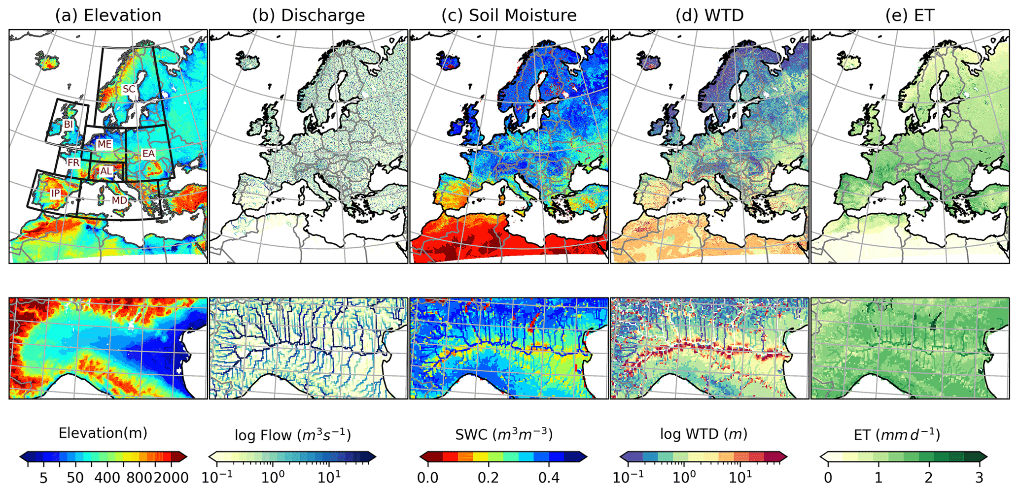
Figure 1Maps of EURO-CORDEX domain at 3 km resolution (1544×1592 grid cells) showing spatially averaged distribution of (a) elevation, (b) discharge, (c) surface soil moisture, (d) water table depth and (e) evapotranspiration (1997–2006), along with close-ups of the Po River basin in the Alpine (AL) region simulated by ParFlow-CLM model. Red color in (d) indicates deeper water table with maximum of 51 m depth. The black boxes in (a) correspond to PRUDENCE regions, with their common abbreviations indicating names of the regions (FR: France; ME: mid-Europe; SC: Scandinavia; EA: eastern Europe; MD: Mediterranean; IP: Iberian Peninsula; BI: the British Isles; AL: Alpine).
2.2 Performance metrics and datasets used for model evaluation
2.2.1 Performance metrics
To assess model performance in simulating hydrological variables, we used percentage bias (PBIAS), Spearman correlation coefficient (R) and modified Kling–Gupta efficiency (KGE'). These metrics were calculated as follows:
where Si and Oi are simulated and observed monthly values, respectively. The PBIAS in Eq. (1) was only calculated for months when observations were available.
The Spearman's rank correlation (R) is a nonparametric measure of correlation which assesses the monotonic relationship between two variables and is therefore less sensitive to outliers. It was calculated as follows:
where di is the difference in paired ranks for a given value of i, and n is the total number of values. For evaluating streamflow, we use the modified Kling–Gupta efficiency metric (KGE'; Gupta et al., 2009; Kling et al., 2012), which is a commonly used measure to assess the similarity between simulated and observed discharge. The modified KGE (KGE') values range from −∞ to 1, where a value of 1 indicates perfect agreement between observations and simulation. It is calculated as follows:
where r is the Pearson correlation coefficient; β and γ are bias ratio and variability ratio, respectively and are calculated as follows:
and
where μs and μo are the mean simulated and observed discharge, and σs and σo are the standard deviation of simulated and observed discharge, respectively.
Using metrics defined in Eqs. (1)–(3), we compared river flow, surface SM, ET, WTD, TWS, and SWE variables with in situ, remote sensing observations and reanalysis datasets to discuss the model performance at different spatial and temporal scales over different regions, as described in Sect. 3. For the regional analysis, the results are presented for eight predefined regions from the “Prediction of Regional scenarios and Uncertainties for Defining European Climate change risks and Effects” (PRUDENCE) project (Christensen and Christensen, 2007), as shown in Fig. 1a, commonly referred to as the “PRUDENCE” regions.
2.2.2 Streamflow data
Daily river flow observations over Europe were obtained from the Global Runoff Data Center (GRDC, obtained via https://www.bafg.de/GRDC/EN/Home/homepage_node.html, last access: 2 May 2018) for more than 2000 gauging stations. Because of the inconsistencies in the real and modeled stream networks due to the relatively coarse resolution of the model grid, the gauging station locations were first adjusted to the nearest locations on the model river network (center of the 0.0275∘ cell). This was accomplished using nearest-neighbor mapping and through comparison of the actual drainage areas with the modeled drainage areas. Only those stations were selected for model validation where drainage area differences were less than 20 % and where more than 50 % of data are available for the time period of 1997–2006. Additionally, we only selected stations where the upstream drainage area is greater than 1000 km2. This resulted in a selection of 176 gauging stations which were then used for comparison with simulated streamflow.
2.2.3 Soil moisture data
The simulated surface SM in the top two layers of the ParFlow-CLM model (∼3 cm) was evaluated by means of comparison with the global satellite observations of SM from the European Space Agency Climate Change Initiative (ESA CCI; Dorigo et al., 2017). The globe ESA CCI SM product was created at 0.25∘ resolution by combining the active and passive microwave sensors, providing a homogeneous and the longest time series of SM data to date, starting from 1979. The dataset has been widely used in various Earth system research studies and has shown good performance in comparison to in situ soil moisture measurements (Gruber et al., 2019). The ParFlow-CLM model results of surface SM were also evaluated with the 3 km European surface SM reanalysis (ESSMRA) datasets (Naz et al., 2020), which were created through assimilation of the ESA CCI data into the land surface model CLM3.5, driven with the same meteorological forcing and static model inputs as those used for ParFlow-CLM. For comparison with model-simulated SM and the ESSMRA dataset, we interpolated the ESA CCI SM data from 0.25 to 0.0275∘ (∼3 km) resolution using the first-order conservative interpolation method (Jones, 1999).
In addition to the satellite-based ESA CCI data, the in situ SM data from the International Soil Moisture Network (ISMN; Dorigo et al., 2011), which provides globally available in situ SM measurements, were also used. Because of the availability of the ISMN SM data covering the study period of 1997–2006, only data from 19 stations from four networks were used for model validation. The surface SM data from these stations for the top 5 cm of surface layer were collected to evaluate the model results in the top two ParFlow-CLM soil layers (about 3 cm). For comparison with model monthly estimates, the measurements with an hourly timescale were aggregated to a monthly timescale. In the case where more than one station was located within one 3 km grid cell, the average of those stations was used for comparison.
2.2.4 Evapotranspiration data
For validation of simulated ET with in situ measurements, ground-based observations of ET were obtained from the FLUXNET2015 dataset (Pastorello et al., 2020), which compiled ecosystem data from the eddy covariance towers. For each FLUXNET site, the latent heat flux (in W m−2) was converted to ET and mm d−1 using the factor of 0.035, assuming , with λ as constant latent heat of vaporization of 2.45 MJ kg−1. For the simulation time period, we used data from 60 FLUXNET sites over Europe, with more than half of the stations concentrated in central Europe (31 out of 60) and only 3 located in eastern Europe.
For evaluation of the model-simulated ET over the pan-European domain, Global Land Surface Satellite (GLASS; Liang et al., 2021) and Global Land Evaporation Amsterdam Model (GLEAM; Martens et al., 2017) datasets were used. The ET data from GLASS are calculated by a multimodel ensemble approach merging five process-based ET datasets (Liang et al., 2013), while GLEAM is based on the water balance method and uses the Priestley–Taylor equation and other algorithms to estimate ET separately for both soil and vegetation (Martens et al., 2017).
2.2.5 Water table depth and total water storage data
To validate the model outputs for WTD, we collected monthly well observations at 5075 groundwater-monitoring wells (Fig. S2 in the Supplement) distributed over Europe from 1997 to 2006. The groundwater level measurements were obtained either from web services or by request from governmental authorities in eight countries (France, Spain, Portugal, the Netherlands, the UK, Sweden, Denmark, and Germany), with most stations concentrated in Germany. The detailed information about the sources of European groundwater-monitoring wells is given in Table S1 in the Supplement. The WTD measurements were first converted to 3 km gridded WTD data by averaging WTD data from all the wells that lie within the same 3 km grid cell. This resulted in 2738 grid cells which were then used to evaluate the ParFlow-CLM results. Reported water table depth data across Europe are poorly quality controlled, with inconsistent methodology and standards employed for the calculation of the depth (Fan et al., 2013). For example, groundwater levels (meters above sea level) are provided for most groundwater-monitoring wells (i.e., 2018 grid cells out of 2738, located mostly in Germany), but no reference surface elevation information is given. This makes it difficult to convert groundwater levels to WTD or to calculate modeled groundwater levels for direct comparison of absolute values. Because of these inconsistencies in reporting water table depth data, we compared the anomalies. Thus, we used standardized anomalies of groundwater table depth in order to remove errors related to the scale mismatch between the simulated groundwater depths and observations and to the differences in reference surface elevations that were used by different countries. The standardized anomalies were calculated for observations and model outputs by first calculating the temporal anomalies and then dividing by the standard deviation of each WTD time series for the time period of 1997–2006. In addition to anomalies, we also compared absolute values of simulated WTD for 720 locations (mostly located in the Netherlands, France and Sweden), where complete WTD data were available.
In addition to WTD, model performance in simulating TWS is evaluated by comparing with satellite-based TWS anomalies from the Gravity Recovery and Climate Experiment (GRACE) with simulated TWS anomalies for the period of 2003–2006. GRACE measures the Earth's gravity field changes and provides global monthly land or terrestrial water storage anomalies, which include water storage anomalies of canopy water, snow water, surface water, soil water and groundwater. In this study, we compared the time series of ParFlow-CLM TWS changes with GRACE release 06 Mascone solution (RL06M) provided by the NASA Jet Propulsion Laboratory (JPL).
2.2.6 Snow water equivalent data
The model-simulated SWE was validated using the GlobSnow (v3.0) reanalysis gridded monthly SWE data which are provided by the European Space Agency. The dataset is available for the Northern Hemisphere (non-mountainous) at 25 km resolution from 1980–2018 (Takala et al., 2011; Pulliainen et al., 2020). The GlobSnow SWE dataset is developed through a data assimilation approach by combining the ground-based synoptic snow depth stations with satellite passive microwave radiometer data and using the HUT snow emission model (Takala et al., 2011). Compared to previous versions of GlobSnow, Luojus et al. (2021) further improved this dataset through bias correction of monthly SWE data using the snow-course SWE measurements independently from the snow depth data used in the assimilation. For comparison with model-simulated SWE, we interpolated the bias-corrected monthly time series of SWE from 25 to 3 km resolution using the first-order conservative interpolation method (Jones, 1999).
The ParFlow-CLM model simulations for the time period of 1997—2006 provide pressure head and saturation values for the variably saturated subsurface layers, as well as energy balance estimates for the land surface at an hourly time step for each grid cell in the study domain. An example of some of the useful downstream model outputs, such as those used for water resource management, are shown in Fig. 1. The top panels show domain extent hydroclimate regions plus elevation and the spatial distribution of mean annual simulated river flow, SM, ET, and WTD. In addition, bottom panels in Fig. 1 show a close-up of the aforementioned variables for the Po River basin in the Alpine region, highlighting the model's ability to resolve small-scale spatial variability in these variables associated with the river network and topography. For WTD, deeper water table values near the large rivers are probably due to the fact that large rivers were carved into the digital elevation model data in order to hydrologically correct the topographic slopes and to ensure European river network connectivity. Enforcement of river network appears to make the valleys more steep, resulting in a deeper WTD in those areas. This is a limitation of the current model setup implementation, which can be improved by using a more advanced approach of topographic processing for integrated hydrologic models (e.g., Condon and Maxwell, 2019a).
In the following section, we discuss the performance of the model for these variables in detail using different performance metrics and comparison with a variety of in situ and remote sensing and reanalysis products. Because of the sparse coverage of in situ observations, comparing with other satellite-based gridded products helps to evaluate model performance for spatial signature over different regions influenced by different (mesoscale) climatic characteristics. Additionally, we compared our results with the CONUS implementation of the ParFlow-CLM model (O'Neill et al., 2021), as summarized in Table S2 in the Supplement. Note that comparisons of our model results with CONUS implementation are limited given the differences in domains, resolution, available observation data (the pan-European domain has more data-sparse areas) and hydroclimate regions. Thus, a direct quantitative comparison is not possible; even so, the model strengths and weaknesses in simulating water states and fluxes are highlighted.
3.1 Streamflow evaluation
ParFlow-CLM streamflow was evaluated against observed monthly river flow for a selection of 176 gauging stations located along many rivers which are mostly concentrated in central Europe (Fig. 2). In evaluating model performance pertaining to mean flow, comparison of the observed and simulated mean flow in the simulation period showed that ParFlow-CLM appropriately reproduced the mean flow, where the PBIAS is below 20 % for 48 % of stations, with only eight stations showing a higher bias (PBIAS>50 %) between the observed and simulated monthly river flow (Fig. 2a). To better understand the seasonal variability of the simulated streamflow, 16 stations along large rivers across different climatic zones, with a total drainage area upstream of the gauging station greater than 5000 km2, were selected and compared with monthly observed streamflows for the simulation period (Fig. 2b). Overall, the comparison shows that the streamflow dynamics are well captured for the selected 16 large rivers; however, there is an overestimation of the winter flow by the model and an underestimation of summer flow for most gauging stations. The overestimation of peak flow is more pronounced in wet years (for example, years 2001 and 2002), whereas low flows in summer are mostly underpredicted in dry years (for example, years 2003 and 2004). The discrepancy between the simulated and observed flow may be related to the following: coarse river resolution in the model and/or human impacts on discharge regimes – particularly for highly regulated rivers through reservoir regulations and power generation or groundwater extraction (e.g., in the case of the Rhine, Elbe, and Danube rivers). In addition, the simulated flow is overpredicted for both River Kemijoki (Finland) and the Nemunas River (Lithuania) in northeastern Europe across all years (Fig. 2a).
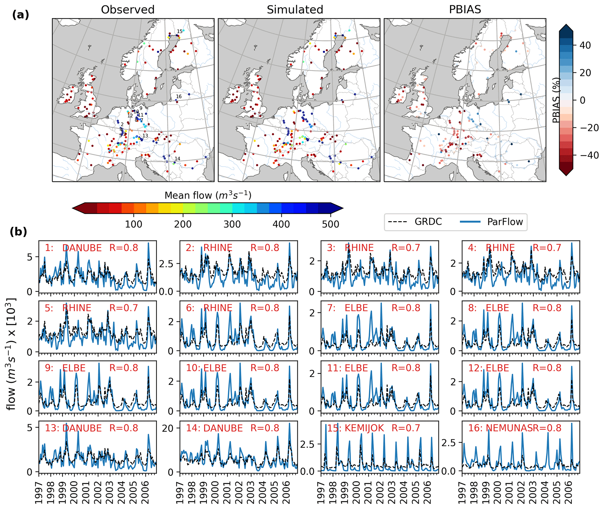
Figure 2(a) Comparison of observed and simulated average discharge and the percentage bias in monthly discharge (PBIAS) for 176 gauging stations. (b) Comparison of time series of observed and simulated discharge for selected large rivers with drainage areas greater than 50 000 km2. Locations of selected gauges in (b) are indicated with corresponding numbers in the left panel of (a).
To further evaluate model performance in terms of streamflow peak times and flow variability, the Spearman correlation coefficient, R, and Kling–Gupta efficiency index, KGE', were calculated for all 176 gauge stations and plotted in Fig. 3. Overall, R and KGE' values ranged from 0.24 to 0.93 and −9.5 to 0.8, respectively, for all 176 stations. ParFlow-CLM performs well for 30 % of stations (54) with a KGE' value greater than 0.5, and only 18 % of basins have a KGE' value less than zero. Regionally, the simulated streamflow results are in good agreement with the observed streamflow over the British Isles, central Europe and France, but model performance in the northern and south eastern regions is relatively poor with KGE' values below zero (Fig. 3b). Comparison of the KGE' and PBIAS shows that a majority of the stations with negative KGE' values have positive biases between the simulated and observed monthly streamflow (Fig. 3c); these are mostly located in northeastern Europe in the EA and SC regions (Fig. 2a). Given that the overprediction of peak flow for northern rivers may also be affected by the overestimation of SWE or from earlier onset of snowmelt in the model, we compared the time-averaged ParFlow-CLM-simulated SWE over winter months with the satellite-based ESA GlobSnow SWE for the low-relief areas (See Fig. S3 in the Supplement). Our comparison shows that ParFlow-CLM simulated higher SWE across the domain, which is particularly noticeable in northeastern Europe. However, it has been shown that GlobSnow data tend to underestimate SWE in the Northern Hemisphere (Luojus et al., 2021), so the overestimation in ParFlow-CLM may not be as large as this comparison suggests. Overall, the ParFlow-CLM northern Europe streamflow performance results agree with previous pan-European studies which showed that most hydrological models perform worse in northeastern Europe, primarily due to forcing data errors and/or a coarse topographic resolution of these models that misrepresent the effects of topography on snow dynamics in these regions (Gudmundsson et al., 2012).
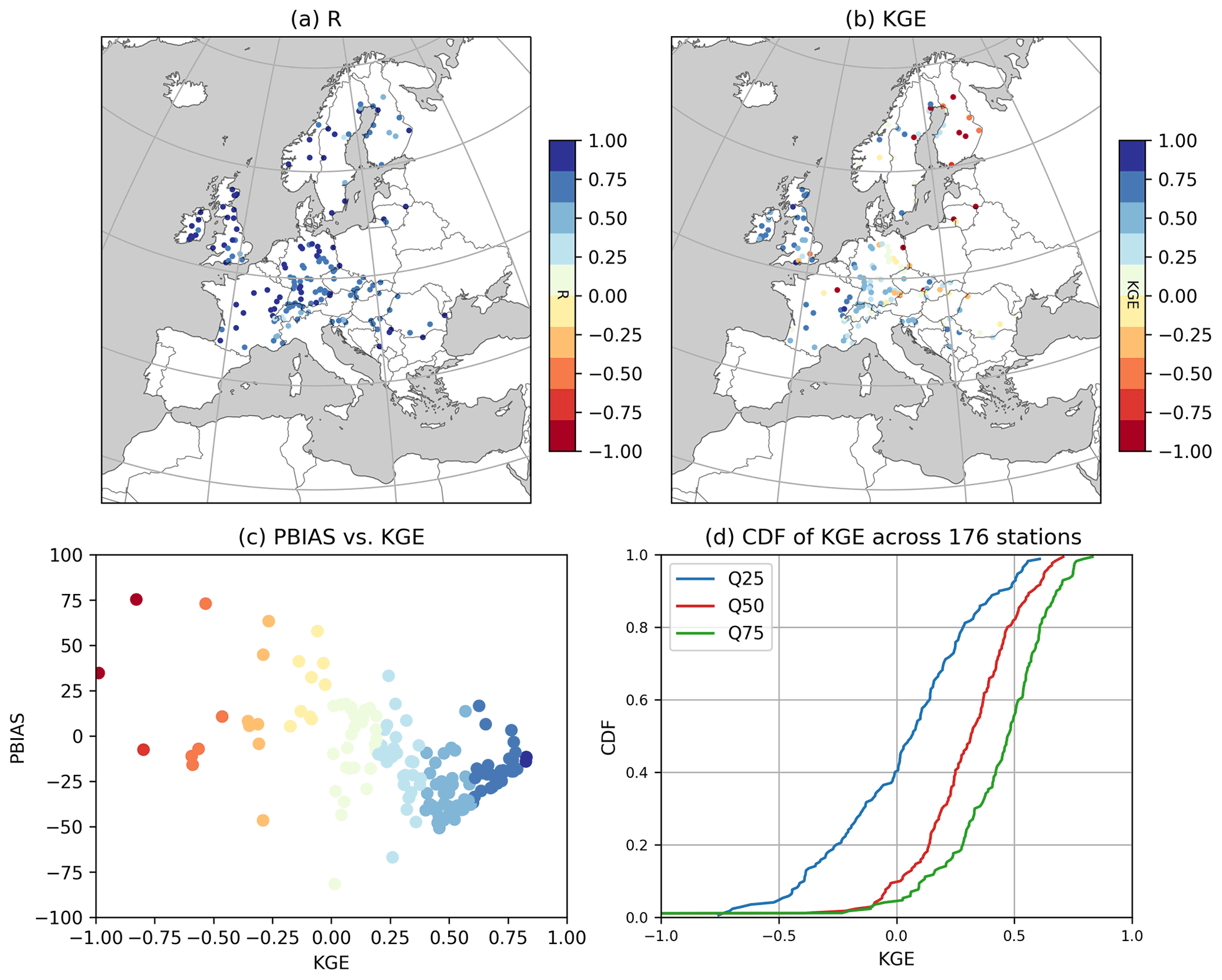
Figure 3Evaluation of ParFlow-CLM-simulated monthly streamflow with observed streamflow for 176 gauging stations. (a) Spearman correlation coefficient (R); (b) modified KGE efficiency index (KGE'); (c) comparison of PBIAS vs. KGE'; (d) cumulative distribution of KGE' for Q50 (between 25th and 75th percentile), Q75 (over 75th percentile) and Q25 (less than 25th percentile) flows. Note that the color code in panel (c) is the same as in (b).
Furthermore, the cumulative distribution of KGE' was calculated separately for medium (between 25th and 75th percentile), high (over 75th percentile) and low (less than 25th percentile) flows to examine ParFlow-CLM's performance in simulating different hydrological characteristics and climate variability, namely, medium, high and low flows. Results show that most stations have higher KGE' values for high flows than for normal and low flows (Fig. 3c). For example, 50 % of stations have KGE' values above 0.5, 0.32 and 0.1 for high, normal and low flows, respectively. The higher-biased gauges are more concentrated towards the eastern domain where the model overestimated peak flows and could be attributed to the higher amount of snow predicted by the ParFlow-CLM model (as shown in Fig. S3). This may indicate that strongly biased gauges in the eastern domain may be a result of positive biases in the meteorological forcing (Goergen and Kollet, 2021). Bollmeyer et al. (2015) compared the COSMO-REA6 precipitation data with the precipitation data from the Global Precipitation Climatology Center, which also showed overestimation of precipitation in northern and eastern European regions (Scandinavia, Russia, and along the Norwegian coast). However, it should be noted that the coverage of gauging stations is very sparse in eastern Europe, and it is difficult to evaluate the reliability of the model results in this part of the domain. Nevertheless, for many of the gauging stations, a relatively good performance of the model for high flow, especially over central Europe, also suggests that the reanalysis meteorological drivers have relatively low precipitation biases over central Europe, as also suggested in Bollmeyer et al. (2015).
Conversely, the strong low-flow biases, which may not be sensitive to variations in first-order precipitation drivers, are more likely to be attributed to factors such as model structural errors or errors in the stream network or model topography. In this context, two factors may contribute to the poor performance of the model for low flows. Firstly, a 3 km grid cell size might still be too coarse to represent realistic stream network of smaller rivers and convergence zones along river corridors. Secondly, ParFlow-CLM allows for a two-way overland flow routing, potentially causing more water losses under dry conditions from channels to groundwater or overbank flow. This may lead to a complete drying of some rivers during summer, further exacerbated by the (comparatively) coarse resolution of the model. Other continental-scale studies that used ParFlow-CLM over the CONUS domain also found underestimation of low flows, particularly in the summer months (O'Neill et al., 2021; Tijerina et al., 2021) where stream segments go dry due to more water losses from the stream channels. A study by Schalge et al. (2019) proposed a method to improve overland flow parameterizations in the ParFlow-CLM model, but more work is needed to identify sources of uncertainties in the overland flow parameters, such as Manning's coefficient or hydraulic conductivity at a continental scale. In any case, an evaluation framework such as this can highlight where model improvements can be undertaken.
3.2 Soil moisture evaluation
To evaluate the ability of ParFlow-CLM to simulate large-scale spatial patterns of surface SM over the study domain, the ParFlow-CLM-simulated SM was compared to ESA CCI datasets (Dorigo et al., 2017). In addition to ESA CCI, we also compared ParFlow-CLM SM with a soil moisture reanalysis dataset (ESSMRA, which is the assimilated soil moisture simulated by CLM3.5; Naz et al., 2020). Surface soil moisture from the ESA CCI dataset was assimilated into the CLM3.5 model to generate the ESSMRA dataset, as described in detail by Naz et al. (2020). We compared ParFlow-CLM SM with the ESSMRA dataset because both models use identical surface information (topography, soil and vegetation) and forcing datasets, and any differences in SM are results of different treatment of groundwater processes or of data assimilation. Since ESSMRA data are available from the year 2000 onward, the comparisons of surface SM from ParFlow-CLM with ESSMRA and ESA CCI were made for the simulation period of 2000–2006. As shown in Fig. 4, ParFlow-CLM shows slightly higher SM than both ESSMRA and ESA CCI over most parts of Europe (humid regions) and underestimates SM in the arid southern areas of the domain. Our comparison of SM simulated by ParFlow-CLM with CLM3.5-simulated SM without any assimilation of ESA CCI (not shown here) also shows positive bias over humid regions. This behavior of the ParFlow-CLM model was seen by O'Neill et al. (2021) over the CONUS domain where the model showed higher surface SM over more humid regions and lower amplitude in the arid southwestern regions relative to the ESA CCI data product. While we cannot rule out biases in other fluxes, it is possible that overestimation of surface SM simulated by ParFlow-CLM could be due to the shallow groundwater system which contributes to the saturation of the deeper soil layers, leading to higher soil water content. In more humid regions, where soils are, in general, wetter, the coupling between groundwater and soil moisture through lateral flow may lead to an overestimation of SM in valleys which may be exacerbated by the (still) coarse resolution of the model with respect to very local hydrologic processes. The influence of resolution on SM has been shown in previous studies – for example, a 3-D groundwater-modeling study where the influence of lateral surface and subsurface flow on SM was more significant at a finer resolution (i.e., <1 km), particularly in wet areas (Ji et al., 2017). Furthermore, Fig. 4b shows the comparison of the spatial distribution of SM simulated by ParFlow-CLM with ESA CCI and ESSMRA as violin plots. The spatial distributions of SM simulated by ParFlow-CLM over PRUDENCE regions show consistently higher SM than both CLM3.5 and ESA CCI, except over the IP region, where SM simulated by ParFlow-CLM is lower than both datasets (Fig. 4b). We observed that the spread of the distribution of ParFlow-CLM SM is quite large when compared to both ESSMRA and ESA CCI in many regions, indicating that higher spatial variability is simulated by ParFlow-CLM. To highlight the differences in spatial variability between the two models (ParFlow-CLM and CLM3.5), we compared the simulated spatially distributed surface soil moisture. We found that the spatial structures simulated by the two models are starkly different (Figs. S4 and S5 in the Supplement). CLM3.5 shows much larger spatial patterns of SM, which are mostly related to the soil properties (e.g., soil texture information), while ParFlow-CLM simulates more spatial variability, which can be attributed to the effects of 3-D flows in river networks and across topography. Note that both models used identical surface information (topography, soil and vegetation) and forcing datasets, indicating that these differences are explained by the fine-scale processes (such as surface and subsurface lateral transport of water movements and the shallow groundwater system) simulated only by ParFlow-CLM. An example is shown in the Supplement for January and August months in 2000 for two regions (Alpine and mid-Europe) with the ESSMRA dataset (Naz et al., 2020) (See Figs. S4 and S5).

Figure 4(a) Evaluation of time-averaged surface soil moisture (SM) simulated by ParFlow-CLM with ESSMRA and ESA CCI datasets over the time period of 2000–2006. (b) Violin plots showing comparison of spatial distribution of time-averaged surface SM simulated by ParFlow-CLM with ESSMRA (upper plot) and ESA CCI (lower plot) over PRUDENCE regions. The violin plots show the estimated kernel density distribution, as well as the median, lower and upper quartiles (white lines). (c) Comparison of spatially aggregated surface SM monthly anomalies estimated by ParFlow-CLM with ESSMRA and ESA CCI datasets for PRUDENCE regions. The SM standardized monthly anomalies in (c) were calculated by subtracting the long-term mean of the complete time series from each month and then dividing by long-term standard deviation for the simulation period of 2000–2006.
To further evaluate model performance in simulating climate variability, namely, simulating average, wet and dry periods, a comparison of monthly time series of SM anomalies at an aggregated regional scale is undertaken. The SM standardized monthly anomalies were calculated by subtracting the long-term mean of the complete time series from each month and then dividing by the long-term standard deviation for the period of 2000–2006. Our results show that ParFlow-CLM agrees well with both ESSMRA and ESA CCI anomalies over the simulation period (Fig. 4c). Upon examination of the R values for different regions, the results show that the correlation of ParFlow-CLM with ESSMRA (red) is higher than with ESA CCI (black) – i.e., R ranging from 0.70 to 0.89 and 0.25 to 0.87 for ESSMRA and ESA CCI, respectively – primarily due to the direct impact of identical forcing used for both modeling setups. Regionally, ParFlow-CLM-simulated SM anomalies agree well with both ESSMRA and ESA CCI for MD, BI, and IP regions (R>0.8). However, in the drought year (2003), ESSMRA shows much stronger dry anomalies than both ParFlow-CLM and ESA CCI (Fig. S6 in the Supplement), suggesting that stronger differences between the models occur during the dry periods. In addition, the low value of R (i.e., 0.25) between ParFlow-CLM and ESA CCI over the Scandinavian region might be due to higher uncertainties in the ESA CCI product for this region, which are observed for regions with limited data, dense vegetation, complex topography and frozen soil (Dorigo et al., 2017). These results are in agreement with the CONUS (O'Neill et al., 2021), which showed lower correlation values for regions with dense vegetation, complex topography, snow cover and frozen soil due to uncertainties in the ESA CCI data for areas with such surface conditions.
The simulated seasonal variability of the monthly volumetric SM content is further evaluated with in situ observations. For the time period of 2000–2006, in situ data from the ISMN network are only available for 41 stations (e.g., Table 3 of Naz et al., 2020) in four countries (France, Spain, Germany and Italy). However, if there is more than one station located within a single 3 km grid cell, then the average of those stations was used, resulting in 19 grid cells for model evaluation over Europe. This comparison demonstrates that both the ESSMRA and ParFlow-CLM models at these locations generally reproduced well the seasonal variability of the surface SM at most stations. For stations with longer observational SM data records (such as SM stations in MOL-RAO in Germany and in the ORACLE network in France), ParFlow-CLM-simulated SM and measured values show better agreement than with the ESSMRA dataset. This might be related to the fact that ParFlow-CLM is better able to resolve small-scale features strongly affected by lateral soil water transport between grid cells and by river network and topography. However, additional in situ observations would be needed to fully evaluate the spatial heterogeneity in surface soil moisture. The comparison is shown in Figs. S7–S10 in the Supplement, which present the monthly time series of the top 5 cm SM from the ParFlow-CLM simulation, ESSMRA and in situ observations for 19 grid cells.
3.3 Evapotranspiration evaluation
Figure 5 compares the simulated monthly ET from ParFlow-CLM with observed ET from 60 eddy covariance tower stations from the FLUXNET database (Pastorello et al., 2020) in order to evaluate the model's ability to capture seasonal ET dynamics. The ParFlow-CLM model performs well and shows reasonable consistency for all stations with respect to monthly ET, with R values greater than 0.6 (Fig. 5a) for all stations. To better understand the agreement between seasonal dynamics of simulated ET with observations, we compared the cumulative distribution of monthly ET for different seasons with observations over all stations in Fig. 5b. The differences between ParFlow-CLM-simulated ET and FLUXNET are smaller for winter (DJF), spring (MAM), and autumn (SON) seasons (on average 0.11, 0.18 and 0.13 mm d−1, respectively) but larger for the summer (JJA) season (0.39 mm d−1) over most stations.
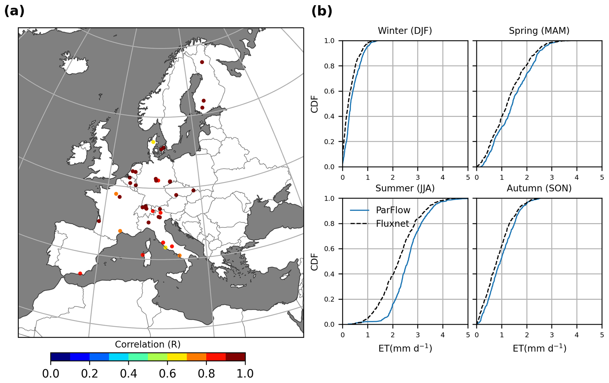
Figure 5Evaluation of ParFlow-CLM-simulated monthly evapotranspiration (ET) with ground-based observations from 60 eddy covariance FLUXNET stations. (b) Comparison of cumulative distribution of seasonal ET estimated by ParFlow-CLM with FLUXNET stations.
During the summer season, the positive ET bias might be due to higher water availability in surface soil for vegetation transpiration and from the bare-soil evaporation simulated by ParFlow-CLM. Previous studies of ParFlow-CLM also indicate that, during dry months, ET is more sensitive to soil resistance parameterization (Jefferson and Maxwell, 2015) and may overestimate ground evaporation when the ground temperatures are higher. Kollet (2009) showed that soil heterogeneities have greater influence on latent heat flux in the ParFlow-CLM model during dry months, and any bias in the soil hydrologic properties such as soil texture, which also determines the hydraulic conductivity values, will likely contribute to ET biases in summer months. Moreover, ET biases can also be attributed to biases in meteorological forcing such as wind speed and vapor pressure. Nevertheless, for most of the stations, the positive bias is relatively small (i.e., +0.39 mm d−1 in summer), and we expect that biases in the soil hydrologic properties and/or in the meteorological forcing are low and do not contribute to any large errors in ET, especially at these locations. While ParFlow-CLM shows acceptable performance for all stations, the relatively small number of stations limits a comprehensive evaluation of model performance over the study domain. Therefore, ParFlow-CLM performance in simulating the spatial variation in ET is further evaluated with the remotely sensed derived GLASS and reanalysis GLEAM datasets. The spatially distributed ET simulated by ParFlow-CLM and its difference compared to both GLASS- and GLEAM-estimated ET are shown in Fig. 6. The ParFlow-CLM-simulated ET is lower than both GLASS and GLEAM ET over most areas in the EURO-CORDEX domain. However, the difference is smaller between ParFlow-CLM and GLEAM ET (i.e., average difference is −0.09 mm d−1) than between ParFlow-CLM and the GLASS ET (i.e., the average difference is about −0.30 mm d−1) over the study domain.
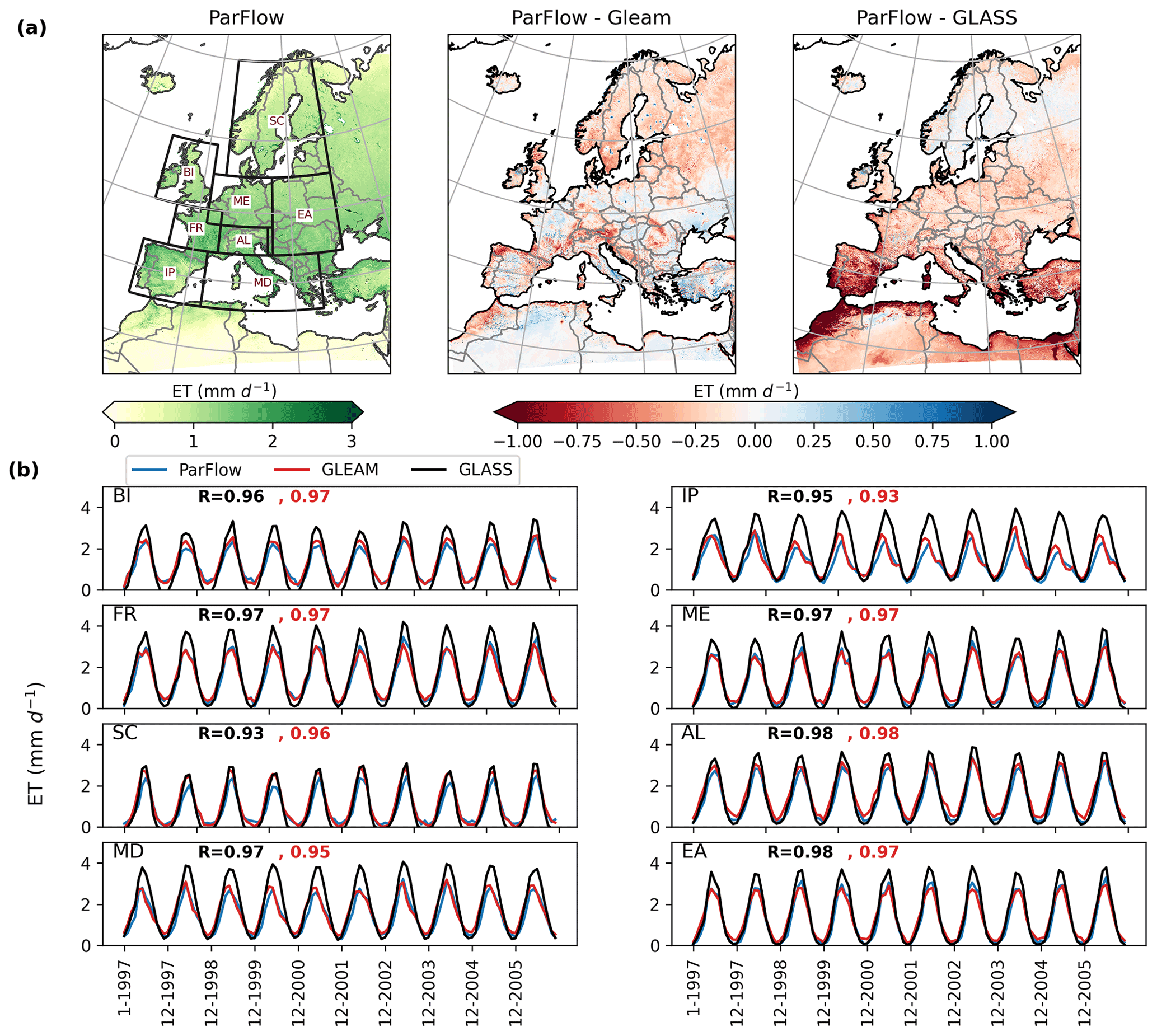
Figure 6(a) Evaluation of time-averaged surface evapotranspiration (ET) simulated by ParFlow-CLM with GLEAM and GLASS datasets over the time period of 1997–2006. (b) Comparison of spatially aggregated monthly ET estimated by ParFlow-CLM with GLEAM and GLASS datasets over PRUDENCE regions (black boxes in a). R values in red color show the correlation of ParFlow-CLM with GLEAM, and R values in black color represent the correlation between ParFlow-CLM and GLASS dataset.
Despite the differences in spatial patterns, the time series of spatially aggregated ET simulated by ParFlow-CLM over PRUDENCE regions is highly correlated with both GLASS (black) and GLEAM (red) datasets (R>0.9), as shown in Fig. 5b. The main differences in ET are mostly detected in summer, where GLASS-estimated ET is larger than both GLEAM- and ParFlow-CLM-simulated ET (Table S3 in the Supplement). But the fact that GLASS has large positive bias over summer when compared with FLUXNET data (Fig. S11 in the Supplement) suggests that GLASS ET data have relatively large uncertainties (Liang et al., 2021). We also note relatively large negative differences upon examination of the GLEAM dataset in areas of complex topography, which may be partly caused by the downscaling of GLEAM data from a coarse spatial resolution (0.25∘).
3.4 Terrestrial water storage and water table depth evaluation
To assess model performance in simulating terrestrial water storage variations, we compared ParFlow-CLM total water storage (TWS) anomalies against GRACE monthly storage anomalies. For the comparison, the TWS anomalies over all storage components (i.e., sum of all surface, subsurface, canopy and snow water stores) from ParFlow-CLM were first calculated for each pixel and then aggregated over PRUDENCE regions. Figure 7 shows the monthly variations in TWS anomaly from both the model and GRACE dataset over eight PRUDENCE regions. Overall, the ParFlow-CLM model represents TWS anomaly adequately well, and a good agreement is achieved for most regions, with correlation values ranging from 0.76–0.91, with higher values being observed in dry regions (i.e., R value of 0.87, 0.85, and 0.91 for IP, FR, and MD, respectively). A relatively lower R is observed in the northern European regions (i.e., R value of 0.74 and 0.76 for BI and SC, respectively). This mismatch could be the result of bias in other simulated variables. For example, ParFlow-CLM underestimates SM anomaly and overestimates ET in the dry regions but overestimates SWE in the snow-dominated regions, as discussed previously. Additionally, the mismatch in TWS anomalies relative to GRACE data can also be partly attributed to uncertainties and errors associated with post-processing and filtering of the coarse-resolution GRACE dataset. Nevertheless, the model performance for TWS over Europe is consistent with findings of other continental-scale hydrologic model studies (e.g., Rakovec et al., 2016; O'Neill et al., 2021).

Figure 7Comparison of monthly time series of total water storage anomalies simulated by ParFlow-CLM with GRACE dataset over PRUDENCE regions.
Furthermore, the ability of ParFlow-CLM to accurately reproduce water table dynamics is evaluated by comparing the simulated WTD anomalies for 2738 grid cells where groundwater-monitoring wells were located. As previously noted, the reference surface elevations provided with the groundwater observational data were not consistent across regions, which makes it difficult to derive the absolute values of WTD for comparison with the model-simulated WTD. Therefore, standardized anomalies were calculated from observed groundwater data in order to reduce errors related to inconsistencies in the observations. Figure 8 shows the temporal correlation coefficients between the monthly time series of WTD anomalies from ParFlow-CLM and observations over Europe. Overall, the ParFlow-CLM model appropriately captures the seasonal cycles with R values above zero for 80 % of locations and 20 % showing satisfactory performance with R>0.5 (inset Fig. 8b). The performance of ParFlow-CLM in simulating WTD anomalies also varies across PRUDENCE regions, with an average R value ranging between 0.21 to 0.34 (Fig. S12 in the Supplement). As an example of ParFlow-CLM performance with the highest and lowest R values across different regions, we showed the time series comparison of selected individual stations (Figs. S13 and S14 in the Supplement). This comparison indicates that the weaker correlations in WTD anomalies by ParFlow-CLM for some locations are related to fewer fluctuations in the observed WTD anomalies in ParFlow-CLM. These discrepancies might be related to uncertainties in aquifer parameterization used in the ParFlow-CLM or to limitations in model resolution such that local aquifers in areas with complex topography cannot be captured. Additionally, model evaluation can be hampered by the challenges associated with groundwater monitoring (e.g., Gleeson et al., 2021). For example, the observations might be biased if they are located towards rivers, in low elevations, in areas with confined or perched aquifer systems, or in coastal areas. The comparison of the resolved simulated head, averaged across 3 km, with the point-scale observation head, which is highly governed by local surface elevation, can bring about misleading results and amplify inaccuracies. Water table depth observations can also be impacted by pumping, which may not be known for many locations and is not captured in the model setup.
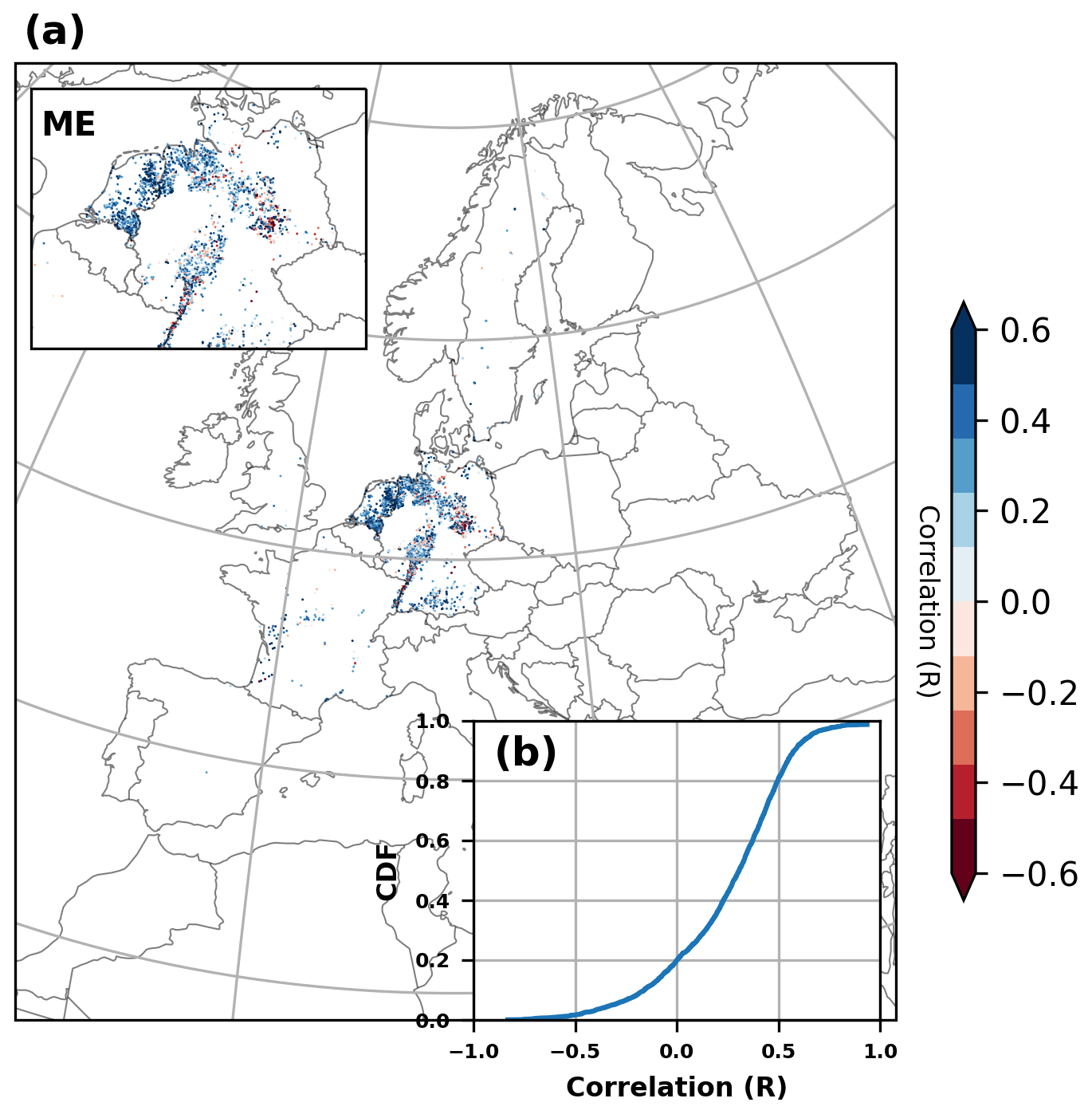
Figure 8(a) Correlation map between in situ water table depth (WTD) anomalies and ParFlow-CLM model. (b) Cumulative distribution function (CDF) of correlation coefficient of ParFlow-CLM with observed WTD anomalies. The inset in (a) shows a zoom of the mid-Europe (ME) region.
To further evaluate model performance in terms of absolute error in the WTD, we compared the model and observations for only those grid cells (720) where complete WTD data are provided and excluded all the other locations. WTD bias for the 720 locations is shown in Fig. 9. For these locations, we found a good agreement between the ParFlow-CLM and observed WTD, with a mean difference of −3.60 m, RMSE of 4.25 m and R value of 0.41. The 25th, 50th and 75th quantiles for simulated minus observed WTD are −2.6, −1.37 and −0.84 m, respectively. Negative values in WTD difference indicate shallower WTD simulated by ParFlow-CLM (i.e., positive bias). However, despite this positive bias, the model is able to capture the temporal dynamics well, with R>0.5 for more than 50 % of locations. Studies by O'Neill et al. (2021) and Maxwell and Condon (2016) over the CONUS domain also found a positive bias in simulated WTD for most well locations, which they found to coincide with aquifers which experienced depletion in groundwater through extractions. In Europe, a few studies also suggest a groundwater decline in past 2 decades, partly related to groundwater abstractions for agriculture and domestic use, particularly in the western and southern European countries (e.g., Xanke and Liesch, 2022); however, in the current study, it is difficult to directly attribute the shallow WTD bias to aquifer depletion because of the sparse observations.
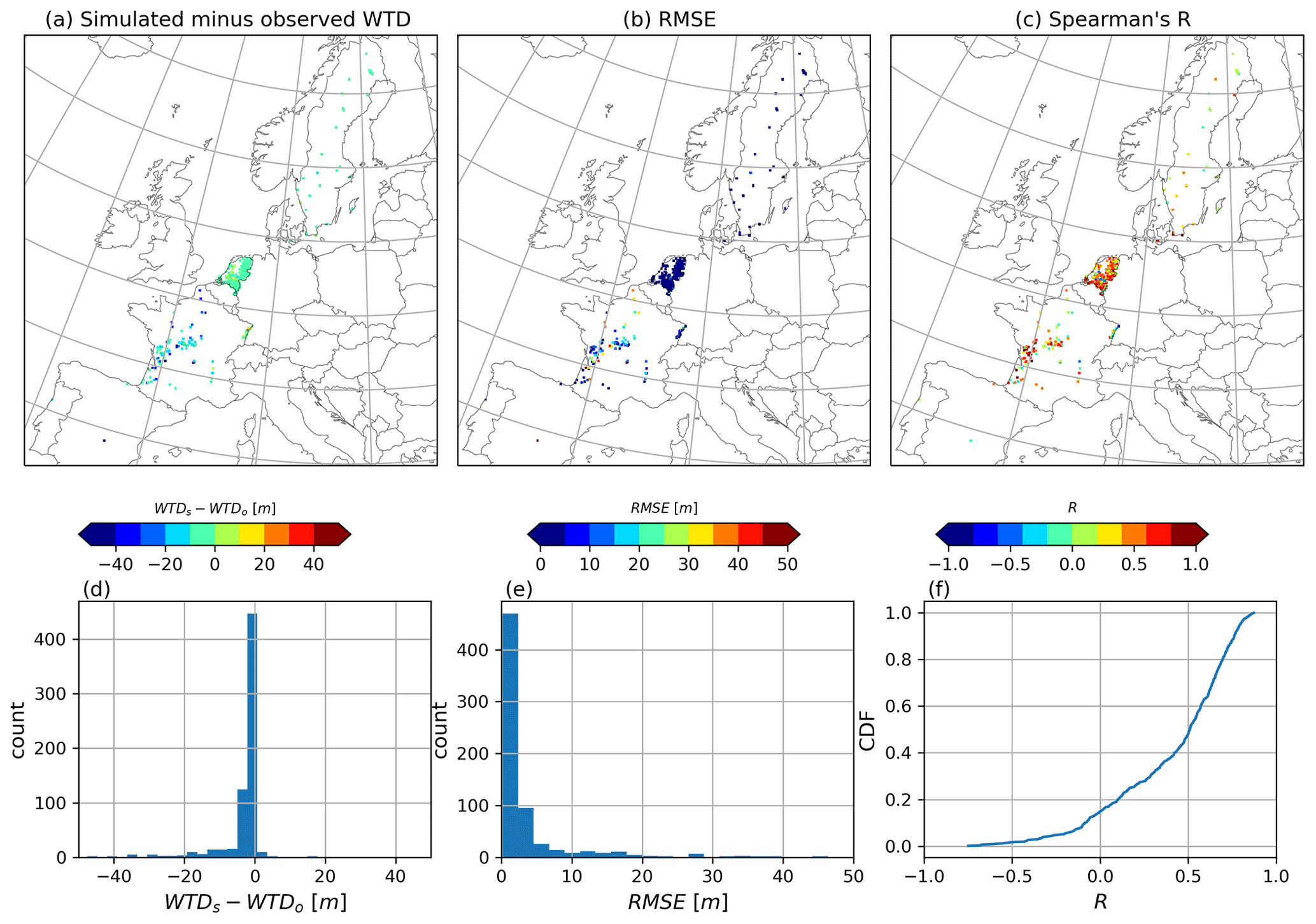
Figure 9(a) Difference in observed and ParFlow-CLM-simulated WTD at filtered locations (N=720), (b) RMSE values at filtered locations and (c) Spearman correlation (R) values at selected locations. Histogram plots show the distribution of (d) simulated minus observed WTD and (e) RMSE values. (f) Cumulative distribution function (CDF) of Spearman correlation of ParFlow-CLM with observed WTD data.
In a changing climate, there is a growing need to apply physically based, fully distributed models at higher resolution over large domains and for long timescales for water security, adaptation and resilience purposes. This study performs an extensive evaluation of a pan-European ParFlow-CLM model to investigate its accuracy and reliability in reproducing high-resolution hydrological states and fluxes over Europe at multiple spatial and temporal scales using a wide range of in situ measurements and remotely sensed observations. While this study was focused mainly on evaluating model performance over a pan-European model domain, it highlights both strengths and limits of the modeling approach, as well as the feasibility of implementing physically based models over a large domain in comparison to simplified models that are more commonly used. For an evaluation period of 10 years, we assess biases in analyzed hydrological variables associated with model inputs, model structure, or observations used for model evaluation, accounting for climate variability and different climate characteristics.
Overall, the model was able to realistically capture the hydrologic behavior (spatial distributions, temporal dynamics, ranges) of different hydrologic variables with reasonable accuracy, as assessed by correlation, relative bias, and Kling–Gupta efficiency metrics. Considering the ParFlow-CLM model was not calibrated for streamflow, the model shows good agreement in simulating river discharge for 176 river basins across Europe (; KGE'>0.5 for 30 % of river basins). Although simulated high flows are comparable with observed discharge, low flows are predominately underestimated. Regionally, the model shows better performance for stream gauges located in central Europe and in the British Isles than for those in northern regions. Our results show that streamflow performance deteriorates in the snow-dominated regions and for highly regulated river basins (e.g., Rhine and Danube river basins). Despite the model's poor performance in simulating discharge for some stations over Europe (especially low flows), the ParFlow-CLM model shows relatively good performance for other variables such as SM, ET and groundwater storage when compared with in situ and remote sensing observations. Overall, the model shows the best agreement, with median R of 0.94 and 0.91, for ET against FLUXNET eddy covariance observations and GLEAM and GLASS datasets, respectively. We found satisfactory performance for other variables, with R values ranging between 0.76 and 0.91 for TWS anomalies relative to the GRACE dataset over PRUDENCE regions, median R of 0.70 for SM relative to ESA CCI, and median R of 0.50 for WTD anomalies relative to groundwater well observations. However, our analysis shows several differences when spatial comparisons were conducted with remotely sensed and reanalysis data products. ParFlow-CLM simulates higher surface SM in comparison to ESA CCI data but shows small differences for ET relative to the GLEAM dataset. It is important to note here that these products are susceptible to errors, which makes the spatial comparisons more challenging. However, when aggregated at the regional scale, ParFlow-CLM shows good agreement for SM, ET, and TWS for semi-arid to arid regions (such as IP, FR, and MD) but shows relatively weak correlations for cold and wetter regions (i.e., BI, ME, SC, and AL). This also suggests that groundwater and lateral surface and subsurface flow maintain wetter soils in arid regions or during dry seasons, thus improving SM, ET, and TWS patterns.
Our results are consistent with a comparable continental-scale study by O'Neill et al. (2021) which evaluated water balance components over the CONUS domain using ParFlow-CLM (PfCONUSv1). While a direct quantitative comparison is not possible due to different domains, resolutions and climatic conditions, we found striking similarities for many variables assessed here. For example, for ET, both model implementations showed overall good agreement against observations but overpredicted ET in the dry regions (e.g., southwest region in CONUS and IP region in Europe) and underpredicted ET in wetter and snow-dominated regions (i.e., in the northern and eastern parts of the CONUS domain and in the SC region in Europe). In addition, both model implementations show an underestimation of ET in mountainous regions, regardless of which product is used for validation. Similarly, for surface soil moisture, both the EU-CORDEX and PfCONUSv1 setups show similar performance, with Spearman correlation (R) values between 0.17–0.77 and 0.25–0.77, respectively, across different regions. Interestingly, both model implementations show an underestimation of surface SM in the arid regions and an overestimation in wetter regions. In terms of storage, both implementations show good agreement for seasonal TWS anomalies relative to GRACE satellite data, but overall, they underpredicted water storage in most areas. For WTD comparison, both model implementations simulated shallower water table depths when compared with groundwater wells data, which could be attributed to the fact that the ParFlow-CLM model does not account for anthropogenic impacts such as groundwater withdrawals, which may lead to overprediction of water table depth in the regions experiencing aquifer depletion (Condon and Maxwell, 2019b). In terms of observation coverage, the CONUS domain consists of a single country and has consistently good coverage. Given that the European model domain consists of many individual countries, observations across regions are not all of the same quality or coverage, which could be a contributing factor for poor model performance in some regions of the EU-CORDEX domain. Nevertheless, the rigorous evaluation of the ParFlow-CLM model over both the EU-CORDEX and CONUS domains paves the way towards a global application of fully distributed, physically based hydrologic models. The protocol of evaluation metrics and methods presented in this study and in O'Neill et al. (2021) can be used as a framework to benchmark future ParFlow-CLM model implementations to further improve model simulations in the areas that have been identified in these studies. For models such as the ParFlow-CLM integrated hydrologic model, which are more complex and therefore more computationally expensive than land surface models or lumped hydrologic models and thus typically not calibrated, quantifying uncertainties in hydrology model simulations is important for further applications such as forecasts or projections.
While this is the first study to provide 10 years of hydrological simulations at 3 km resolution over Europe using a fully distributed ParFlow-CLM model with lateral groundwater flow representation, some inevitable limitations in the model implementation of this study should be noted. First, uncertainties in the static input data (such as hydrogeological information, land cover and soil information) can contribute to errors in the model. While we use the best available consistent datasets as a whole for Europe (and globally as well), in this study, we did not analyze the contribution of errors in hydrological variables that come from uncertainties in the model input datasets. As the quality of these inputs increases, so too will the simulations. Similarly, while the meteorological forcings used in this study (COSMO-REA6) are produced through the assimilation of observational meteorological data, the quality of the data in some data-sparse regions (e.g., in eastern Europe) may suffer from inaccuracies. The COSMO-REA6 is, to our knowledge, the only high-resolution reanalysis dataset for all of Europe available as of today. Our comparison of simulated SWE with RS observations reveals an overprediction of SWE in the eastern regions, which is more likely to be related to the uncertainties in forcing datasets or model structure errors in simulating the snow and energy balance. Using an ensemble atmospheric forcing dataset would be highly desirable, albeit computationally expensive.
Second, in this study, we did not address the uncertainties in the model parameters that are required for model simulations, such as hydraulic conductivity, porosity, and soil and vegetation parameters, which may introduce biases in our results. Because of the associated computational cost of ParFlow-CLM, studies of the sensitivity of water balance variables to these parameters are difficult. With the ongoing model developments and collaborative efforts to improve the computational efficiency of ParFlow with its GPU version (e.g., Hokkanen et al., 2021) and ensemble-based sensitivity analysis tools (e.g., Friedemann and Raffin, 2022), it will be possible in the future to also conduct continental-scale ensemble-based sensitivity analyses for quantifying model parameter uncertainties.
In this study, comparison with observations to evaluate the ParFlow-CLM model's performance provides first-order confidence of the model's ability to realistically simulate multiple hydro-climates, along with climate variability, across multiple water balance components in a pan-European domain. The results from this study can also be used as a baseline for future ParFlow-CLM implementations over Europe. Future work will consist of extending the dataset out to recent years, which will allow us to evaluate model outputs with more recent high-resolution RS products. Further research should also focus on inter-model comparison analysis of a coarser-resolution implementation of ParFlow-CLM or other land surface models without lateral flow for further tuning of the model parameters or to identify sources of uncertainties in model outputs related to the effects of groundwater and surface water lateral flow.
The latest version of the open-source ParFlow-CLM is freely available on GitHub at https://github.com/parflow/parflow.git (last access: 30 June 2022). The ParFlow-CLM version 3.6 used in this study is archived on Zenodo at https://doi.org/10.5281/zenodo.4639761 (Smith et al., 2019). The model outputs, which are approximately 20 TB of data (including atmospheric forcings and post-processed outputs), are available upon request. Selected model outputs are available at https://doi.org/10.5281/zenodo.7716900 (Naz, 2023). The run control framework used in this study is archived at https://doi.org/10.5281/zenodo.1303424 (Sharples, 2018).
The supplement related to this article is available online at: https://doi.org/10.5194/gmd-16-1617-2023-supplement.
BSN, WS, KG, and SK designed the study. BSN and WS conducted the experiments. YM helped with collection and post-processing of water table depth data from groundwater-monitoring wells. BSN prepared the paper with contributions from the co-authors. All authors have read and agreed to the published version of the paper.
The contact author has declared that none of the authors has any competing interests.
Publisher's note: Copernicus Publications remains neutral with regard to jurisdictional claims in published maps and institutional affiliations.
The authors gratefully acknowledge the computing time granted through JARA on the supercomputer JURECA (Jülich Supercomputing Centre, 2021) at Forschungszentrum Jülich. In addition, we acknowledge the supercomputing support and the computational and storage resources provided to us by the Jülich Supercomputing Center (JSC) through the Simulation and Data Laboratory Terrestrial Systems of the Center for High-Performance Scientific Computing in Terrestrial Systems (Geoverbund ABC/J, https://www.hpsc-terrsys.de, last access: 15 December 2021, and the JSC, Germany). The authors also thank the editor and anonymous reviewers for their constructive feedback during the review process.
This research has been supported by the European Commission, Horizon 2020 Framework Programme (EoCoE-II (grant no. 824158)), and the Deutsche Forschungsgemeinschaft (DFG, German Research Foundation) – SFB 1502/1–2022 – project number 450058266.
The article processing charges for this open-access publication were covered by the Forschungszentrum Jülich.
This paper was edited by Charles Onyutha and reviewed by Stefano Ferraris and three anonymous referees.
Ashby, S. F. and Falgout, R. D.: A Parallel Multigrid Preconditioned Conjugate Gradient Algorithm for Groundwater Flow Simulations, Nucl. Sci. Eng., 124, 145–159, https://doi.org/10.13182/NSE96-A24230, 1996. a
Barlage, M., Chen, F., Rasmussen, R., Zhang, Z., and Miguez-Macho, G.: The Importance of Scale-Dependent Groundwater Processes in Land-Atmosphere Interactions Over the Central United States, Geophys. Res. Lett., 48, e2020GL092171, https://doi.org/10.1029/2020GL092171, 2021. a, b
Barnes, M. L., Welty, C., and Miller, A. J.: Global Topographic Slope Enforcement to Ensure Connectivity and Drainage in an Urban Terrain, J. Hydrol. Eng., 21, 06015017, https://doi.org/10.1061/(ASCE)HE.1943-5584.0001306, 2016. a
Batjes, N. H.: A world dataset of derived soil properties by FAO–UNESCO soil unit for global modelling, Soil Use Manage., 13, 9–16, 1997. a
Beven, K. J. and Cloke, H. L.: Comment on “Hyperresolution global land surface modeling: Meeting a grand challenge for monitoring Earth's terrestrial water” by Eric F. Wood et al., Water Resour. Res., 48, W01801, https://doi.org/10.1029/2011WR010982, 2012. a
Bierkens, M. F., Bell, V. A., Burek, P., Chaney, N., Condon, L. E., David, C. H., de Roo, A., Döll, P., Drost, N., and Famiglietti, J. S.: Hyper-resolution global hydrological modelling: what is next? “Everywhere and locally relevant”, Hydrol. Process., 29, 310–320, 2015. a
Bollmeyer, C., Keller, J. D., Ohlwein, C., Wahl, S., Crewell, S., Friederichs, P., Hense, A., Keune, J., Kneifel, S., and Pscheidt, I.: Towards a high-resolution regional reanalysis for the European CORDEX domain, Q. J. Roy. Meteor. Soc., 141, 1–15, 2015. a, b, c
Bouaziz, L. J. E., Fenicia, F., Thirel, G., de Boer-Euser, T., Buitink, J., Brauer, C. C., De Niel, J., Dewals, B. J., Drogue, G., Grelier, B., Melsen, L. A., Moustakas, S., Nossent, J., Pereira, F., Sprokkereef, E., Stam, J., Weerts, A. H., Willems, P., Savenije, H. H. G., and Hrachowitz, M.: Behind the scenes of streamflow model performance, Hydrol. Earth Syst. Sci., 25, 1069–1095, https://doi.org/10.5194/hess-25-1069-2021, 2021. a
Burstedde, C., Fonseca, J. A., and Kollet, S.: Enhancing speed and scalability of the ParFlow simulation code, Comput. Geosci., 22, 347–361, https://doi.org/10.1007/s10596-017-9696-2, 2018. a
Christensen, J. H. and Christensen, O. B.: A summary of the PRUDENCE model projections of changes in European climate by the end of this century, Climatic Change, 81, 7–30, 2007. a
Clark, M. P., Fan, Y., Lawrence, D. M., Adam, J. C., Bolster, D., Gochis, D. J., Hooper, R. P., Kumar, M., Leung, L. R., Mackay, D. S., Maxwell, R. M., Shen, C., Swenson, S. C., and Zeng, X.: Improving the representation of hydrologic processes in Earth System Models, Water Resour. Res., 51, 5929–5956, https://doi.org/10.1002/2015WR017096, 2015. a
Clark, M. P., Bierkens, M. F. P., Samaniego, L., Woods, R. A., Uijlenhoet, R., Bennett, K. E., Pauwels, V. R. N., Cai, X., Wood, A. W., and Peters-Lidard, C. D.: The evolution of process-based hydrologic models: historical challenges and the collective quest for physical realism, Hydrol. Earth Syst. Sci., 21, 3427–3440, https://doi.org/10.5194/hess-21-3427-2017, 2017. a
Condon, L. E. and Maxwell, R. M.: Evaluating the relationship between topography and groundwater using outputs from a continental-scale integrated hydrology model: Evaluating Groundwater Controls, Water Resour. Res., 51, 6602–6621, https://doi.org/10.1002/2014WR016774, 2015. a
Condon, L. E. and Maxwell, R. M.: Systematic shifts in Budyko relationships caused by groundwater storage changes, Hydrol. Earth Syst. Sci., 21, 1117–1135, https://doi.org/10.5194/hess-21-1117-2017, 2017. a
Condon, L. E. and Maxwell, R. M.: Modified priority flood and global slope enforcement algorithm for topographic processing in physically based hydrologic modeling applications, Comput. Geosci., 126, 73–83, https://doi.org/10.1016/j.cageo.2019.01.020, 2019a. a
Condon, L. E. and Maxwell, R. M.: Simulating the sensitivity of evapotranspiration and streamflow to large-scale groundwater depletion, Sci. Adv., 5, eaav4574, https://doi.org/10.1126/sciadv.aav4574, 2019b. a
Condon, L. E., Kollet, S., Bierkens, M. F. P., Fogg, G. E., Maxwell, R. M., Hill, M. C., Fransen, H.-J. H., Verhoef, A., Van Loon, A. F., Sulis, M., and Abesser, C.: Global Groundwater Modeling and Monitoring: Opportunities and Challenges, Water Resour. Res., 57, e2020WR029500, https://doi.org/10.1029/2020WR029500, 2021. a
Dai, Y., Zeng, X., Dickinson, R. E., Baker, I., Bonan, G. B., Bosilovich, M. G., Denning, A. S., Dirmeyer, P. A., Houser, P. R., and Niu, G.: The common land model, B. Am. Meteorol. Soc., 84, 1013–1024, 2003. a
Danielson, J. J. and Gesch, D. B.: Global Multi-resolution Terrain Elevation Data 2010 (GMTED2010), GMTED2010 [data set], 34, U.S. Gelogical Survey, https://doi.org/10.3133/ofr20111073, 2010. a
de Graaf, I., Condon, L., and Maxwell, R.: Hyper-Resolution Continental-Scale 3-D Aquifer Parameterization for Groundwater Modeling, Water Resour. Res., 56, e2019WR026004, https://doi.org/10.1029/2019WR026004, 2020. a, b
Döll, P., Kaspar, F., and Lehner, B.: A global hydrological model for deriving water availability indicators: model tuning and validation, J. Hydrol., 270, 105–134, https://doi.org/10.1016/S0022-1694(02)00283-4, 2003. a, b
Dorigo, W., Wagner, W., Albergel, C., Albrecht, F., Balsamo, G., Brocca, L., Chung, D., Ertl, M., Forkel, M., and Gruber, A.: ESA CCI Soil Moisture for improved Earth system understanding: State-of-the art and future directions, Remote Sens. Environ., 203, 185–215, 2017. a, b, c
Dorigo, W. A., Wagner, W., Hohensinn, R., Hahn, S., Paulik, C., Xaver, A., Gruber, A., Drusch, M., Mecklenburg, S., van Oevelen, P., Robock, A., and Jackson, T.: The International Soil Moisture Network: a data hosting facility for global in situ soil moisture measurements, Hydrol. Earth Syst. Sci., 15, 1675–1698, https://doi.org/10.5194/hess-15-1675-2011, 2011. a
Duscher, K., Günther, A., Richts, A., Clos, P., Philipp, U., and Struckmeier, W.: The GIS layers of the “International Hydrogeological Map of Europe 1 : 1 500 000” in a vector format, Hydrogeol. J., 23, 1867–1875, https://doi.org/10.1007/s10040-015-1296-4, 2015. a
Fan, Y.: Groundwater in the Earth's critical zone: Relevance to large-scale patterns and processes, Water Resour. Res., 51, 3052–3069, https://doi.org/10.1002/2015WR017037, 2015. a
Fan, Y., Li, H., and Miguez-Macho, G.: Global patterns of groundwater table depth, Science, 339, 940–943, 2013. a
Friedemann, S. and Raffin, B.: An elastic framework for ensemble-based large-scale data assimilation, Int. J. High Perform. C., 36, 543–563, https://doi.org/10.1177/10943420221110507, 2022. a
Friedl, M. A., McIver, D. K., Hodges, J. C., Zhang, X. Y., Muchoney, D., Strahler, A. H., Woodcock, C. E., Gopal, S., Schneider, A., and Cooper, A.: Global land cover mapping from MODIS: algorithms and early results, Remote Sens. Environ., 83, 287–302, 2002. a
Furusho-Percot, C., Goergen, K., Hartick, C., Kulkarni, K., Keune, J., and Kollet, S.: Pan-European groundwater to atmosphere terrestrial systems climatology from a physically consistent simulation, Scientific Data, 6, 320, https://doi.org/10.1038/s41597-019-0328-7, 2019. a
Gleeson, T., Moosdorf, N., Hartmann, J., and van Beek, L. P. H.: A glimpse beneath earth's surface: GLobal HYdrogeology MaPS (GLHYMPS) of permeability and porosity, Geophys. Res. Lett., 41, 3891–3898, https://doi.org/10.1002/2014GL059856, 2014. a
Gleeson, T., Wagener, T., Döll, P., Zipper, S. C., West, C., Wada, Y., Taylor, R., Scanlon, B., Rosolem, R., Rahman, S., Oshinlaja, N., Maxwell, R., Lo, M.-H., Kim, H., Hill, M., Hartmann, A., Fogg, G., Famiglietti, J. S., Ducharne, A., de Graaf, I., Cuthbert, M., Condon, L., Bresciani, E., and Bierkens, M. F. P.: GMD perspective: The quest to improve the evaluation of groundwater representation in continental- to global-scale models, Geosci. Model Dev., 14, 7545–7571, https://doi.org/10.5194/gmd-14-7545-2021, 2021. a
Goergen, K. and Kollet, S.: Boundary condition and oceanic impacts on the atmospheric water balance in limited area climate model ensembles, Sci. Rep.-UK, 11, 6228, https://doi.org/10.1038/s41598-021-85744-y, 2021. a
Grimaldi, S., Schumann, G. J., Shokri, A., Walker, J. P., and Pauwels, V. R. N.: Challenges, Opportunities, and Pitfalls for Global Coupled Hydrologic-Hydraulic Modeling of Floods, Water Resour. Res., 55, 5277–5300, https://doi.org/10.1029/2018WR024289, 2019. a
Gruber, A., Scanlon, T., van der Schalie, R., Wagner, W., and Dorigo, W.: Evolution of the ESA CCI Soil Moisture climate data records and their underlying merging methodology, Earth Syst. Sci. Data, 11, 717–739, https://doi.org/10.5194/essd-11-717-2019, 2019. a
Gudmundsson, L., Wagener, T., Tallaksen, L. M., and Engeland, K.: Evaluation of nine large-scale hydrological models with respect to the seasonal runoff climatology in Europe, Water Resour. Res., 48, W11504, https://doi.org/10.1029/2011WR010911, 2012. a, b, c
Gupta, H. V., Kling, H., Yilmaz, K. K., and Martinez, G. F.: Decomposition of the mean squared error and NSE performance criteria: Implications for improving hydrological modelling, J. Hydrol., 377, 80–91, https://doi.org/10.1016/j.jhydrol.2009.08.003, 2009. a
Gutowski Jr., W. J., Giorgi, F., Timbal, B., Frigon, A., Jacob, D., Kang, H.-S., Raghavan, K., Lee, B., Lennard, C., Nikulin, G., O'Rourke, E., Rixen, M., Solman, S., Stephenson, T., and Tangang, F.: WCRP COordinated Regional Downscaling EXperiment (CORDEX): a diagnostic MIP for CMIP6, Geosci. Model Dev., 9, 4087–4095, https://doi.org/10.5194/gmd-9-4087-2016, 2016. a
Haddeland, I., Clark, D. B., Franssen, W., Ludwig, F., Voß, F., Arnell, N. W., Bertrand, N., Best, M., Folwell, S., Gerten, D., Gomes, S., Gosling, S. N., Hagemann, S., Hanasaki, N., Harding, R., Heinke, J., Kabat, P., Koirala, S., Oki, T., Polcher, J., Stacke, T., Viterbo, P., Weedon, G. P., and Yeh, P.: Multimodel Estimate of the Global Terrestrial Water Balance: Setup and First Results, J. Hydrometeorol., 12, 869–884, https://doi.org/10.1175/2011JHM1324.1, 2011. a, b
Hanel, M., Rakovec, O., Markonis, Y., Máca, P., Samaniego, L., Kyselý, J., and Kumar, R.: Revisiting the recent European droughts from a long-term perspective, Sci. Rep.-UK, 8, 9499, https://doi.org/10.1038/s41598-018-27464-4, 2018. a
Hartick, C., Furusho-Percot, C., Goergen, K., and Kollet, S.: An Interannual Probabilistic Assessment of Subsurface Water Storage Over Europe Using a Fully Coupled Terrestrial Model, Water Res., 57, e2020WR027828, https://doi.org/10.1029/2020WR027828, 2021. a
He, K., Yang, Q., Shen, X., and Anagnostou, E. N.: Brief communication: Western Europe flood in 2021 – mapping agriculture flood exposure from synthetic aperture radar (SAR), Nat. Hazards Earth Syst. Sci., 22, 2921–2927, https://doi.org/10.5194/nhess-22-2921-2022, 2022. a
Hengl, T., Mendes de Jesus, J., Heuvelink, G. B. M., Gonzalez, M. R., Kilibarda, M., Blagotić, A., Shangguan, W., Wright, M. N., Geng, X., Bauer-Marschallinger, B., Guevara, M. A., Vargas, R., MacMillan, R. A., Batjes, N. H., Leenaars, J. G. B., Ribeiro, E., Wheeler, I., Mantel, S., and Kempen, B.: SoilGrids250m: Global gridded soil information based on machine learning, PLOS One, 12, e0169748, https://doi.org/10.1371/journal.pone.0169748, 2017. a
Hill, M. C. and Tiedeman, C. R.: Effective Groundwater Model Calibration: With Analysis of Data, Sensitivities, Predictions, and Uncertainty, John Wiley & Sons, google-Books-ID: N2wHI1rUpkQC, Print ISBN 9780471776369, Online ISBN 9780470041086, https://doi.org/10.1002/0470041080, 2006. a
Hokkanen, J., Kollet, S., Kraus, J., Herten, A., Hrywniak, M., and Pleiter, D.: Leveraging HPC accelerator architectures with modern techniques – hydrologic modeling on GPUs with ParFlow, Comput. Geosci., 25, 1579–1590, https://doi.org/10.1007/s10596-021-10051-4, 2021. a
Hunger, M. and Döll, P.: Value of river discharge data for global-scale hydrological modeling, Hydrol. Earth Syst. Sci., 12, 841–861, https://doi.org/10.5194/hess-12-841-2008, 2008. a
Jacob, D., Teichmann, C., Sobolowski, S., Katragkou, E., Anders, I., Belda, M., Benestad, R., Boberg, F., Buonomo, E., Cardoso, R. M., Casanueva, A., Christensen, O. B., Christensen, J. H., Coppola, E., De Cruz, L., Davin, E. L., Dobler, A., Domínguez, M., Fealy, R., Fernandez, J., Gaertner, M. A., García-Díez, M., Giorgi, F., Gobiet, A., Goergen, K., Gómez-Navarro, J. J., Alemán, J. J. G., Gutiérrez, C., Gutiérrez, J. M., Güttler, I., Haensler, A., Halenka, T., Jerez, S., Jiménez-Guerrero, P., Jones, R. G., Keuler, K., Kjellström, E., Knist, S., Kotlarski, S., Maraun, D., van Meijgaard, E., Mercogliano, P., Montávez, J. P., Navarra, A., Nikulin, G., de Noblet-Ducoudré, N., Panitz, H.-J., Pfeifer, S., Piazza, M., Pichelli, E., Pietikäinen, J.-P., Prein, A. F., Preuschmann, S., Rechid, D., Rockel, B., Romera, R., Sánchez, E., Sieck, K., Soares, P. M. M., Somot, S., Srnec, L., Sørland, S. L., Termonia, P., Truhetz, H., Vautard, R., Warrach-Sagi, K., and Wulfmeyer, V.: Regional climate downscaling over Europe: perspectives from the EURO-CORDEX community, Reg. Environ. Change, 20, 51, https://doi.org/10.1007/s10113-020-01606-9, 2020. a
Jefferson, J. L. and Maxwell, R. M.: Evaluation of simple to complex parameterizations of bare ground evaporation, J. Adv. Model. Earth Sy., 7, 1075–1092, https://doi.org/10.1002/2014MS000398, 2015. a, b
Jefferson, J. L., Gilbert, J. M., Constantine, P. G., and Maxwell, R. M.: Active subspaces for sensitivity analysis and dimension reduction of an integrated hydrologic model, Comput. Geosci., 83, 127–138, https://doi.org/10.1016/j.cageo.2015.07.001, 2015. a
Jefferson, J. L., Maxwell, R. M., and Constantine, P. G.: Exploring the Sensitivity of Photosynthesis and Stomatal Resistance Parameters in a Land Surface Model, J. Hydrometeorol., 18, 897–915, https://doi.org/10.1175/JHM-D-16-0053.1, 2017. a, b
Ji, P., Yuan, X., and Liang, X.-Z.: Do Lateral Flows Matter for the Hyperresolution Land Surface Modeling?, J. Geophys. Res.-Atmos., 122, 12077–12092, https://doi.org/10.1002/2017JD027366, 2017. a, b, c, d
Jones, J. E. and Woodward, C. S.: Newton–Krylov-multigrid solvers for large-scale, highly heterogeneous, variably saturated flow problems, Adv. Water Resour., 24, 763–774, 2001. a, b
Jones, P. W.: First-and second-order conservative remapping schemes for grids in spherical coordinates, Mon. Weather Rev., 127, 2204–2210, 1999. a, b
Jülich Supercomputing Centre: JURECA: Data Centric and Booster Modules implementing the Modular Supercomputing Architecture at Jülich Supercomputing Centre, Journal of Large-Scale Research Facilities, 7, A182, https://doi.org/10.17815/jlsrf-7-182, 2021. a
Keune, J., Gasper, F., Goergen, K., Hense, A., Shrestha, P., Sulis, M., and Kollet, S.: Studying the influence of groundwater representations on land surface-atmosphere feedbacks during the European heat wave in 2003, J. Geophys. Res.-Atmos., 121, 13301–13325, https://doi.org/10.1002/2016JD025426, 2016. a, b, c, d
Keune, J., Sulis, M., and Kollet, S. J.: Potential Added Value of Incorporating Human Water Use on the Simulation of Evapotranspiration and Precipitation in a Continental-Scale Bedrock-to-Atmosphere Modeling System: A Validation Study Considering Observational Uncertainty, J. Adv. Model. Earth Syst., 11, 1959–1980, https://doi.org/10.1029/2019MS001657, 2019. a, b
Kling, H., Fuchs, M., and Paulin, M.: Runoff conditions in the upper Danube basin under an ensemble of climate change scenarios, J. Hydrol., 424–425, 264–277, https://doi.org/10.1016/j.jhydrol.2012.01.011, 2012. a
Kollet, S., Gasper, F., Brdar, S., Goergen, K., Hendricks-Franssen, H.-J., Keune, J., Kurtz, W., Küll, V., Pappenberger, F., Poll, S., Trömel, S., Shrestha, P., Simmer, C., and Sulis, M.: Introduction of an Experimental Terrestrial Forecasting/Monitoring System at Regional to Continental Scales Based on the Terrestrial Systems Modeling Platform (v1.1.0), Water, 10, 1697, https://doi.org/10.3390/w10111697, 2018. a
Kollet, S. J.: Influence of soil heterogeneity on evapotranspiration under shallow water table conditions: Transient, stochastic simulations, Environ. Res. Lett., 4, 035007, https://doi.org/10.1088/1748-9326/4/3/035007, 2009. a
Kollet, S. J. and Maxwell, R. M.: Integrated surface–groundwater flow modeling: A free-surface overland flow boundary condition in a parallel groundwater flow model, Adv. Water Resour., 29, 945–958, 2006. a
Kollet, S. J. and Maxwell, R. M.: Capturing the influence of groundwater dynamics on land surface processes using an integrated, distributed watershed model, Water Resour. Res., 44, W02402, https://doi.org/10.1029/2007WR006004, 2008. a, b
Kollet, S. J., Maxwell, R. M., Woodward, C. S., Smith, S., Vanderborght, J., Vereecken, H., and Simmer, C.: Proof of concept of regional scale hydrologic simulations at hydrologic resolution utilizing massively parallel computer resources, Water Resour. Res., 46, W04201, https://doi.org/10.1029/2009WR008730, 2010. a
Kuffour, B. N. O., Engdahl, N. B., Woodward, C. S., Condon, L. E., Kollet, S., and Maxwell, R. M.: Simulating coupled surface–subsurface flows with ParFlow v3.5.0: capabilities, applications, and ongoing development of an open-source, massively parallel, integrated hydrologic model, Geosci. Model Dev., 13, 1373–1397, https://doi.org/10.5194/gmd-13-1373-2020, 2020. a, b
Lawrence, D. M., Fisher, R. A., Koven, C. D., Oleson, K. W., Swenson, S. C., Bonan, G., Collier, N., Ghimire, B., van Kampenhout, L., Kennedy, D., Kluzek, E., Lawrence, P. J., Li, F., Li, H., Lombardozzi, D., Riley, W. J., Sacks, W. J., Shi, M., Vertenstein, M., Wieder, W. R., Xu, C., Ali, A. A., Badger, A. M., Bisht, G., van den Broeke, M.., Brunke, M. A., Burns, S. P., Buzan, J., Clark, M., Craig, A., Dahlin, K., Drewniak, B., Fisher, J. B., Flanner, M., Fox, A. M., Gentine, P., Hoffman, F., Keppel-Aleks, G., Knox, R., Kumar, S., Lenaerts, J., Leung, L. R., Lipscomb, W. H., Lu, Y., Pandey, A., Pelletier, J. D., Perket, J., Randerson, J. T., Ricciuto, D. M., Sanderson, B. M., Slater, A., Subin, Z. M., Tang, J., Thomas, R. Q., Martin, M. V., and Zeng, X.: The Community Land Model Version 5: Description of New Features, Benchmarking, and Impact of Forcing Uncertainty, J. Adv. Model. Earth Sy., 11, 4245–4287, https://doi.org/10.1029/2018MS001583, 2019. a
Liang, S., Zhang, X., Xiao, Z., Cheng, J., Liu, Q., and Zhao, X.: Global LAnd Surface Satellite (GLASS) Products: Algorithms, Validation and Analysis, Springer Science & Business Media, ISBN 978-3-319-02588-9, 2013. a
Liang, S., Cheng, J., Jia, K., Jiang, B., Liu, Q., Xiao, Z., Yao, Y., Yuan, W., Zhang, X., Zhao, X., and Zhou, J.: The Global Land Surface Satellite (GLASS) Product Suite, B. Am. Meteorol. Soc., 102, E323–E337, https://doi.org/10.1175/BAMS-D-18-0341.1, 2021. a, b
Luojus, K., Pulliainen, J., Takala, M., Lemmetyinen, J., Mortimer, C., Derksen, C., Mudryk, L., Moisander, M., Hiltunen, M., Smolander, T., Ikonen, J., Cohen, J., Salminen, M., Norberg, J., Veijola, K., and Venäläinen, P.: GlobSnow v3.0 Northern Hemisphere snow water equivalent dataset, Sci. Data, 8, 163, https://doi.org/10.1038/s41597-021-00939-2, 2021. a, b
Martens, B., Miralles, D. G., Lievens, H., van der Schalie, R., de Jeu, R. A. M., Fernández-Prieto, D., Beck, H. E., Dorigo, W. A., and Verhoest, N. E. C.: GLEAM v3: satellite-based land evaporation and root-zone soil moisture, Geosci. Model Dev., 10, 1903–1925, https://doi.org/10.5194/gmd-10-1903-2017, 2017. a, b
Martínez-de la Torre, A. and Miguez-Macho, G.: Groundwater influence on soil moisture memory and land–atmosphere fluxes in the Iberian Peninsula, Hydrol. Earth Syst. Sci., 23, 4909–4932, https://doi.org/10.5194/hess-23-4909-2019, 2019. a
Maxwell, R. M.: A terrain-following grid transform and preconditioner for parallel, large-scale, integrated hydrologic modeling, Adv. Water Resour., 53, 109–117, 2013. a
Maxwell, R. M. and Condon, L. E.: Connections between groundwater flow and transpiration partitioning, Science, 353, 377–380, https://doi.org/10.1126/science.aaf7891, 2016. a, b, c, d
Maxwell, R. M. and Kollet, S. J.: Interdependence of groundwater dynamics and land-energy feedbacks under climate change, Nat. Geosci., 1, 665, 2008. a
Maxwell, R. M., Condon, L. E., and Kollet, S. J.: A high-resolution simulation of groundwater and surface water over most of the continental US with the integrated hydrologic model ParFlow v3, Geosci. Model Dev., 8, 923–937, https://doi.org/10.5194/gmd-8-923-2015, 2015. a, b
Miguez-Macho, G. and Fan, Y.: The role of groundwater in the Amazon water cycle: 1. Influence on seasonal streamflow, flooding and wetlands: Amazon Groundwater-Surface Water Link, J. Geophys. Res.-Atmos., 117, D15113, https://doi.org/10.1029/2012JD017539, 2012. a
Miguez-Macho, G., Fan, Y., Weaver, C. P., Walko, R., and Robock, A.: Incorporating water table dynamics in climate modeling: 2. Formulation, validation, and soil moisture simulation, J. Geophys. Res.-Atmos., 112, 2006JD008112, https://doi.org/10.1029/2006JD008112, 2007. a
Naz, B. S.: 3 km ParFlow-CLM model simulations over EU-CORDEX, Zenodo [data set], https://doi.org/10.5281/zenodo.7716900, 2023. a
Naz, B. S., Kollet, S., Franssen, H.-J. H., Montzka, C., and Kurtz, W.: A 3 km spatially and temporally consistent European daily soil moisture reanalysis from 2000 to 2015, Sci. Data, 7, 111, https://doi.org/10.1038/s41597-020-0450-6, 2020. a, b, c, d, e
Oleson, K. W., Niu, G.-Y., Yang, Z.-L., Lawrence, D. M., Thornton, P. E., Lawrence, P. J., Stöckli, R., Dickinson, R. E., Bonan, G. B., and Levis, S.: Improvements to the Community Land Model and their impact on the hydrological cycle, J. Geophys. Res.-Biogeo., 113, G01021, https://doi.org/10.1029/2007JG000563, 2008. a
O'Neill, M. M. F., Tijerina, D. T., Condon, L. E., and Maxwell, R. M.: Assessment of the ParFlow–CLM CONUS 1.0 integrated hydrologic model: evaluation of hyper-resolution water balance components across the contiguous United States, Geosci. Model Dev., 14, 7223–7254, https://doi.org/10.5194/gmd-14-7223-2021, 2021. a, b, c, d, e, f, g, h, i, j, k, l, m, n
Pastorello, G., Trotta, C., Canfora, E. et al.: The FLUXNET2015 dataset and the ONEFlux processing pipeline for eddy covariance data, Sci. Data, 7, 225, https://doi.org/10.1038/s41597-020-0534-3, 2020. a, b
Pokhrel, Y., Felfelani, F., Satoh, Y., Boulange, J., Burek, P., Gädeke, A., Gerten, D., Gosling, S. N., Grillakis, M., Gudmundsson, L., Hanasaki, N., Kim, H., Koutroulis, A., Liu, J., Papadimitriou, L., Schewe, J., Müller Schmied, H., Stacke, T., Telteu, C.-E., Thiery, W., Veldkamp, T., Zhao, F., and Wada, Y.: Global terrestrial water storage and drought severity under climate change, Nat. Clim. Change, 11, 226–233, https://doi.org/10.1038/s41558-020-00972-w, 2021. a
Pulliainen, J., Luojus, K., Derksen, C., Mudryk, L., Lemmetyinen, J., Salminen, M., Ikonen, J., Takala, M., Cohen, J., Smolander, T., and Norberg, J.: Patterns and trends of Northern Hemisphere snow mass from 1980 to 2018, Nature, 581, 294–298, https://doi.org/10.1038/s41586-020-2258-0, 2020. a
Rafiei, V., Nejadhashemi, A. P., Mushtaq, S., Bailey, R. T., and An-Vo, D.-A.: An improved calibration technique to address high dimensionality and non-linearity in integrated groundwater and surface water models, Environ. Modell. Softw., 149, 105312, https://doi.org/10.1016/j.envsoft.2022.105312, 2022. a
Rakovec, O., Kumar, R., Mai, J., Cuntz, M., Thober, S., Zink, M., Attinger, S., Schäfer, D., Schrön, M., and Samaniego, L.: Multiscale and Multivariate Evaluation of Water Fluxes and States over European River Basins, J. Hydrometeorol., 17, 287–307, https://doi.org/10.1175/JHM-D-15-0054.1, 2016. a, b
Rakovec, O., Samaniego, L., Hari, V., Markonis, Y., Moravec, V., Thober, S., Hanel, M., and Kumar, R.: The 2018–2020 Multi-Year Drought Sets a New Benchmark in Europe, Earths Future, 10, e2021EF002394, https://doi.org/10.1029/2021EF002394, 2022. a
Reinecke, R., Foglia, L., Mehl, S., Trautmann, T., Cáceres, D., and Döll, P.: Challenges in developing a global gradient-based groundwater model (G3M v1.0) for the integration into a global hydrological model, Geosci. Model Dev., 12, 2401–2418, https://doi.org/10.5194/gmd-12-2401-2019, 2019. a
Ryken, A., Bearup, L. A., Jefferson, J. L., Constantine, P., and Maxwell, R. M.: Sensitivity and model reduction of simulated snow processes: Contrasting observational and parameter uncertainty to improve prediction, Adv. Water Resour., 135, 103473, https://doi.org/10.1016/j.advwatres.2019.103473, 2020. a
Scanlon, B. R., Zhang, Z., Save, H., Sun, A. Y., Müller Schmied, H., van Beek, L. P. H., Wiese, D. N., Wada, Y., Long, D., Reedy, R. C., Longuevergne, L., Döll, P., and Bierkens, M. F. P.: Global models underestimate large decadal declining and rising water storage trends relative to GRACE satellite data, P. Natl. Acad. Sci. USA, 115, E1080–E1089, https://doi.org/10.1073/pnas.1704665115, 2018. a
Schaap, M. G. and Leij, F. J.: Database-related accuracy and uncertainty of pedotransfer functions, Soil Sci., 163, 765–779, 1998. a, b
Schalge, B., Haefliger, V., Kollet, S., and Simmer, C.: Improvement of surface run-off in the hydrological model ParFlow by a scale-consistent river parameterization, Hydrol. Process., 33, 2006–2019, https://doi.org/10.1002/hyp.13448, 2019. a
Schwingshackl, C., Hirschi, M., and Seneviratne, S. I.: Quantifying Spatiotemporal Variations of Soil Moisture Control on Surface Energy Balance and Near-Surface Air Temperature, J. Climate, 30, 7105–7124, https://doi.org/10.1175/JCLI-D-16-0727.1, 2017. a
Sellers, P. J., Mintz, Y., Sud, Y. C., and Dalcher, A.: A Brief Description of the Simple Biosphere Model (SiB), in: Physically-Based Modelling and Simulation of Climate and Climatic Change: Part 1, edited by: Schlesinger, M. E., NATO ASI Series, Springer Netherlands, Dordrecht, 307–330, https://doi.org/10.1007/978-94-009-3041-4_7, 1988. a
Sharples, W.: The run control framework, data, and version of ParFlow used in the publication: A run control framework to streamline profiling, porting, and tuning simulation runs and provenance tracking of geoscientific applications, Zenodo [data set], https://doi.org/10.5281/zenodo.1303424, 2018. a
Shrestha, P., Sulis, M., Masbou, M., Kollet, S., and Simmer, C.: A scale-consistent terrestrial systems modeling platform based on COSMO, CLM, and ParFlow, Mon. Weather Rev., 142, 3466–3483, 2014. a
Shrestha, P., Sulis, M., Simmer, C., and Kollet, S.: Impacts of grid resolution on surface energy fluxes simulated with an integrated surface-groundwater flow model, Hydrol. Earth Syst. Sci., 19, 4317–4326, https://doi.org/10.5194/hess-19-4317-2015, 2015. a
Shrestha, P., Sulis, M., Simmer, C., and Kollet, S.: Effects of horizontal grid resolution on evapotranspiration partitioning using TerrSysMP, J. Hydrol., 557, 910–915, https://doi.org/10.1016/j.jhydrol.2018.01.024, 2018. a
Simmer, C., Adrian, G., Jones, S., Wirth, V., Göber, M., Hohenegger, C., Janjic, T., Keller, J., Ohlwein, C., and Seifert, A.: Herz: The german hans-ertel centre for weather research, B. Am. Meteorol. Soc., 97, 1057–1068, 2016. a
Smith, S., Maxwell, R., Condon, L., Engdahl, N., Gasper, F., Kulkarni, K., Beisman, J., Hector, B., Woodward, C., Fonseca, J., Thompson, D., and Coon, E.: ParFlow Version 3.6.0 (Version v3.6.0), Zenodo [code], https://doi.org/10.5281/zenodo.4639761, 2019. a
Takala, M., Luojus, K., Pulliainen, J., Derksen, C., Lemmetyinen, J., Kärnä, J.-P., Koskinen, J., and Bojkov, B.: Estimating northern hemisphere snow water equivalent for climate research through assimilation of space-borne radiometer data and ground-based measurements, Remote Sens. Environ., 115, 3517–3529, https://doi.org/10.1016/j.rse.2011.08.014, 2011. a, b
Tijerina, D., Condon, L., FitzGerald, K., Dugger, A., O'Neill, M. M., Sampson, K., Gochis, D., and Maxwell, R.: Continental Hydrologic Intercomparison Project, Phase 1: A Large-Scale Hydrologic Model Comparison Over the Continental United States, Water Resour. Res., 57, e2020WR028931, https://doi.org/10.1029/2020WR028931, 2021. a, b
Tolley, D., Foglia, L., and Harter, T.: Sensitivity Analysis and Calibration of an Integrated Hydrologic Model in an Irrigated Agricultural Basin With a Groundwater-Dependent Ecosystem, Water Resour. Res., 55, 7876–7901, https://doi.org/10.1029/2018WR024209, 2019. a
Verkaik, J., Sutanudjaja, E. H., Oude Essink, G. H. P., Lin, H. X., and Bierkens, M. F. P.: GLOBGM v1.0: a parallel implementation of a 30 arcsec PCR-GLOBWB-MODFLOW global-scale groundwater model, Geosci. Model Dev. Discuss. [preprint], https://doi.org/10.5194/gmd-2022-226, in review, 2022. a
Vogt, J., Soille, P., De Jager, A., Rimaviciute, E., Mehl, W., Foisneau, S., Bodis, K., Dusart, J., Paracchini, M. L., and Haastrup, P.: A pan-European river and catchment database, European Commission, EUR, 22920, 120, https://doi.org/10.2788/35907, 2007. a
Wood, E. F., Roundy, J. K., Troy, T. J., van Beek, L. P. H., Bierkens, M. F. P., Blyth, E., de Roo, A., Döll, P., Ek, M., Famiglietti, J., Gochis, D., van de Giesen, N., Houser, P., Jaffé, P. R., Kollet, S., Lehner, B., Lettenmaier, D. P., Peters-Lidard, C., Sivapalan, M., Sheffield, J., Wade, A., and Whitehead, P.: Hyperresolution global land surface modeling: Meeting a grand challenge for monitoring Earth's terrestrial water, Water Resour. Res., 47, W05301, https://doi.org/10.1029/2010WR010090, 2011. a
Xanke, J. and Liesch, T.: Quantification and possible causes of declining groundwater resources in the Euro-Mediterranean region from 2003 to 2020, Hydrogeol. J., 30, 379–400, https://doi.org/10.1007/s10040-021-02448-3, 2022. a
Xie, Z., Di, Z., Luo, Z., and Ma, Q.: A Quasi-Three-Dimensional Variably Saturated Groundwater Flow Model for Climate Modeling, J. Hydrometeorol., 13, 27–46, https://doi.org/10.1175/JHM-D-10-05019.1, 2012. a
Zeng, Y., Xie, Z., Liu, S., Xie, J., Jia, B., Qin, P., and Gao, J.: Global Land Surface Modeling Including Lateral Groundwater Flow, J. Adv. Model. Earth Sy., 10, 1882–1900, https://doi.org/10.1029/2018MS001304, 2018. a, b
Zhou, X., Zhang, Y., Wang, Y., Zhang, H., Vaze, J., Zhang, L., Yang, Y., and Zhou, Y.: Benchmarking global land surface models against the observed mean annual runoff from 150 large basins, J. Hydrol., 470–471, 269–279, https://doi.org/10.1016/j.jhydrol.2012.09.002, 2012. a