Reproducible and relocatable regional ocean modelling: fundamentals and practices

In response to an increasing demand for bespoke or tailored regional ocean modelling configurations, we outline fundamental principles and practices that can expedite the process to generate new configurations. The paper develops the principle of reproducibility and advocates adherence by presenting benefits to the community and user. The elements of this principle are reproducible workflows and standardised assessment, with additional effort over existing working practices being balanced against the added value generated. The paper then decomposes the complex build process, for a new regional ocean configuration, into stages and presents guidance, advice and insight for each component. This advice is compiled from across the NEMO (Nucleus for European Modelling of the Ocean) user community and sets out principles and practises that encompass regional ocean modelling with any model. With detailed and region-specific worked examples in Sects. 3 and 4, the linked companion repositories and DOIs all target NEMOv4. The aim of this review and perspective paper is to broaden the user community skill base and to accelerate development of new configurations in order to increase the time available for exploiting the configurations.

1 Introduction

There is internationally an increasing demand for simulations of the marine environment to deepen our understanding of the marine system and its sensitivities in a changing climate. High-profile issues include marine hazards from storms (Harley et al., 2022; Masselink et al., 2016), sea level rise (Fox-Kemper et al., 2021; Ponte et al., 2019), management of blue carbon resources and understanding the potential marine impacts of climate change mitigation interventions, such as marine offshore renewable energy (Dorrell et al., 2022) and land use change (Felgate et al., 2021).

While global ocean modelling products and research activities are increasing in resolution and sophistication, they are still a long way from the scale and process representation required to deliver accurate information on the coastal ocean. There are a number of reasons why it is advantageous to configure bespoke regional models: though data catalogues like the Copernicus Marine Service (CMS: https://marine.copernicus.eu, last access: 20 February 2023, and others) are rich resources for regional and global marine data, these cannot always satisfy all user requirements. Motivations need not always be about spatial resolution. For example, missing processes can be an important driver for building a new configuration (perhaps addressing a lack of integrated physics and biogeochemistry or a lack of tidal processes in the “off-the-shelf” catalogue products). Alternatively, bespoke model outputs might be required (such as high-frequency output for specific sub-regions or new metrics). So, the key advantages of regional over global configurations include benefits associated with resolution enhancements, design flexibility and computational efficiency (to contain only the region and processes that matter and to not worry about degrading the solution in other regions). On the other hand, key disadvantages include the need for lateral boundary conditions (which can be hard to obtain and a potential source of error), the human resources required to configure and maintain multiple regional domains, and the lack of a common experience across a global community of coastal ocean modellers.

The configuration of a regional ocean model has traditionally been a one-off event taking many months and requiring many, often subtle, expert decisions. Consequently, descriptions of the set-up (e.g. in the literature) are relatively limited or hard to reproduce in their entirety. The need to configure multiple regional models in many different seas around the world has led us to develop a systematic workflow where NEMO (the Nucleus for European Modelling of the Ocean, Madec and Team, 2022, http://www.nemo-ocean.eu, last access: 20 February 2023) regional ocean configurations could be more efficiently built, deployed and reproduced. This reproducible workflow is not intended to be the sole authority on regional configuration set-ups or to provide a turn-key or black-box solution; instead, it is designed to provide a set of guidelines for modellers to follow in order to capitalise on the usability and interoperability of the resulting simulations. Indeed, other modelling systems, such as the Massachusetts Institute of Technology general circulation model, MITgcm (Marshall et al., 1997), the Regional Ocean Modeling System, ROMS (Shchepetkin and McWilliams, 2005) and the Finite Volume Community Ocean Model, FVCOM (Chen et al., 2006), can also be readily configured for new regional applications. All have their own strengths which are largely set according to the model system's development history and the user's familiarity with the system. For example, ROMS was specifically designed as a regional ocean model, and MITgcm has been a model of choice for numerous idealised process studies. On the other hand, FVCOM's unstructured mesh has made it a popular research code choice for multi-scale coastal hydrodynamics. The concepts presented here are intended to be broadly applicable to any modelling system, though the worked examples are implemented within NEMO.

NEMO is an ocean modelling framework underpinned by a consortium of five large European research, climate and operational centres. It is well supported as an international community modelling code and consequently is employed as the ocean component for 9 of the 35 widely used Coupled Model Intercomparison Project Phase 6 (CMIP6) models (Eyring et al., 2016, https://pcmdi.llnl.gov/CMIP6/, last access: 27 July 2022) and is used in the CMS catalogue of freely available marine data products. As a regional model it benefits substantially from these investments of effort. However, its origins in large research and operational centres (where teams focus on specific configurations) has led, quite naturally, to barriers to NEMO being more widely used in regional applications.

In our experience, each research question addressed with a regional model configuration requires a subtly different workflow. Sometimes this would be the requirement of different forcing, sometimes the use of ensemble simulations, or sometimes different domain files. The intention here, therefore, is not to provide a manual on how to build a configuration but instead to share the concepts that need to be considered and practices that can be utilised when building a new configuration. This is in part done with code examples. Note that the intention is not to create an automatic method for generating new configurations (e.g. Trotta et al., 2021); NEMO is a continually evolving code base with frequent releases and updates, so any turn-key solution would be quickly depreciated and less appropriate for cutting-edge scientific endeavours. Furthermore, since the process as a whole is complex and an unwelcome barrier to new starters, we have found it instructive to offer recipes that guide the user through the stages that need to be considered. Users are then encouraged to modify these recipes for their own purposes, gaining insight by doing so whilst simultaneously preserving the reproducibility documentation.

On this journey we have developed methodologies that reinforce the principle of reproducibility, which is fundamental to the scientific method. In particular, these practices are aimed at making large modelling frameworks more accessible. These concepts and benefits are discussed in Sect. 2. In Sect. 3 we step through the important considerations that can guide the construction of a new regional configuration. Model- and configuration-specific details are abstracted into worked examples in linked repositories. In Sect. 4 important considerations are described for a selection of modules that can expand the suite of process representation beyond the hydrodynamics (i.e. biogeochemistry, waves, nested domains, and ice processes). Finally, discussions and conclusions are in Sect. 5. The paper is specifically targeted at the NEMO framework, with the hope of thereby making NEMO a more accessible framework for regional ocean modelling. However, the concepts (if not the details) are readily transferable to any regional modelling system.

2 Reproducibility: a fundamental principle and its implementation and sustainability

The scientific method requires reproducibility. However, there is no defined level of documentation or code sharing required to meet this requirement. Here we specifically consider the activities required to reproduce a simulation on the assumption that the numerical solution is independent of the discretisation implementation (e.g. machine architecture, processor decomposition, or grid orientation, which are handled by the modelling framework developers). In our discipline, code has always been available on request from authors, but with increasingly complex code bases, significant levels of expert knowledge are increasingly required to be able to compile and implement the code. The established modelling frameworks such as the MITgcm (https://mitgcm.org/documentation/, last access: 9 February 2023), ROMS (https://www.myroms.org/wiki/Documentation_Portal, last access: 9 February 2023) and NEMO (https://www.nemo-ocean.eu, last access: 9 February 2023) all have comprehensive documentation, with large self-supporting user communities and online forums. Within the NEMO framework this support is invaluable for new users getting started and for community engagement with system development. However, this alone cannot deliver reproducibility, which arguably is minimally implemented within our community.

It is easy to understand how the additional time burden and potential loss of “intellectual property” might disincentivise an individual in making their science too easy to reproduce. Indeed, the strategy for how one chooses to make their work reproducible, or the level one must attain, is not prescribed, and perhaps nor should it be. However, this lack of prescription and the non-trivial amount of expert knowledge required to generate or reproduce simulations can enhance the barrier to new adoption of modelling frameworks.

Beyond being a mandate, reproducibility offers clear benefits to the community. Reproducibility leads to enhanced efficiency, with less time “reinventing the wheel” or consumed by software problems and more time dedicated to science discovery or project deliverables. Reproducibility can lead to a democratisation of skills across a user base and an upskilling for individuals. It can accelerate debugging and therefore accelerate development. Enhanced levels of reproducibility in existing configurations make delivery of new working configurations a realistic prospect within smaller research projects and furthermore make the process more accessible to new regional modellers.

Furthermore, with the progression towards increasingly automated and integrated systems (e.g. https://www.ukri.org/wp-content/uploads/2022/05/NERC-170522-NERCDigitalStrategy-FINAL-WEB.pdf, last access: 9 February 2023), there will be an increasing demand for machine-capable reproducibility.

In recent years, and in response to an increasing demand for new regional configurations, the authors sought to develop such practices. The concepts outlined here are intended to transcend code versions and even modelling frameworks. They are emergent rather than novel, born and distilled from experience and intending to borrow good working practices from the software development community. To be effective, they must be memorable, even obvious.

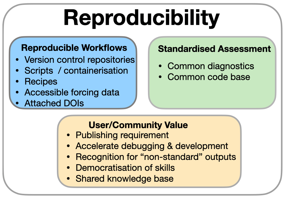
Figure 1 The principle of reproducibility is delivered by reproducible workflows and standardised assessment, but this ideal can only be maintained when its contribution is understood and valued.

There are three elements that have precipitated out of our work towards reproducibility (and we are still on the journey). There are two activities, reproducible workflows and standardised assessment, and a third element, value. For the endeavour to be sustainable, the additional activities must produce a recognisable value that exceeds the effort. Schematically summarised in Fig. 1, these are each addressed in the following.

2.1 Reproducible configurations

The first activity within the enhanced reproducibility principle is reproducible workflows (Fig. 1). Reproducible relocatable regional modelling workflows already exist. Indeed, established and alternative workflows should be reviewed and considered when choosing a template appropriate for a new project. Seminal examples include the following.

• A Structured and Unstructured grid Relocatable ocean platform for Forecasting (SURF: Trotta et al., 2016, 2021, https://www.surf-platform.org/tutorial.php, laast access: 1 July 2022), also using NEMO (and unstructured modelling) to rapidly build and deploy configurations for real-time maritime disaster response. The focus is on operational deployment and reliability. This necessitates a high level of automation and reliance on mature code versions.

• The NEMO nowcast framework (https://nemo-nowcast.readthedocs.io/en/latest/, access: 1 July 2022). This is a well-documented collection of Python modules that can be used to build a software system to run the NEMO ocean model in a daily nowcast/forecast mode. NEMO nowcast has different, though complementary, ambitions for this paper but is likely to be of interest to the reader.

• The Salish Sea MEOPAR project documentation (https://salishsea-meopar-docs.readthedocs.io/en/latest/code-notes/salishsea-nemo/index.html, last access: 1 July 2022). This includes extensive documentation for a regionally specific NEMO configuration of the Canadian Salish Sea, which is deployed in various research projects (e.g. Soontiens and Allen, 2017).

Guided by existing examples and our own experiences, in this section the focus is on workflows that can enhance reproducibility whilst maintaining scientific flexibility.

2.1.1 Organised workflows

The key route to effective workflow reproducibility and its benefits is via systematic documentation.

Central to the structure advocated here is the use of the following.

• i.

  Version control repositories for modifications to the standard NEMO source code. We arbitrarily choose git and GitHub.

• ii.

  Scripts for configuring parts of the set-up that can be automated and labour-saving. These also reside in the git repositories.

• iii.

  Recipes to describe the whole process.

It was found that the recipes, which make the whole process transparent from software installation through to assessment and analysis, were especially important in democratising the build process. Even though they took some time to document, the benefit was immediate since multiple scientists and students could independently work on projects without continual reliance on overburdened NEMO specialists.

Documenting the whole process in detail was important since the recipes form a template for subsequent configurations, for which the required modifications are hard to anticipate and could vary in nature from high-performance-computing (HPC) architecture changes to alternative boundary forcing data.

We found the https://github.com (last access: 20 February 2023) platform convenient for workflow management, since the code modifications, scripts and recipes (the latter being in the form of associated wikis) could be co-located under one repository. We also found that the design of an “optimal” template repository was elusive since our various projects and experiments had subtly different requirements, making a universal template unwieldy. We found, therefore, that the most efficient approach to getting the benefits of an accelerated start on new projects was to clone and modify an existing project.

Excellent (and inspirational) examples of this workflow include the long-standing and extensive Canadian Salish Sea MEOPAR project documentation. In the UK the requirements have not been geographically focused and so led to an emphasis on building new relocatable configurations, starting with Lighthouse Reef in Belize (https://pynemo.readthedocs.io/en/latest/examples.html, last access: 6 January 2023) as a demonstrator. Subsequently this was iterated to build early versions of the SEAsia repository (https://doi.org/10.5281/zenodo.6483231, Polton et al., 2022a), which in turn spawned Caribbean (https://doi.org/10.5281/zenodo.3228088, Wilson et al., 2019), which was modified to have scripts to auto-build and run clean prescribed experiments using data recovery from remote storage (https://jasmin.ac.uk, last access: 20 February 2023) and compute on a remote HPC resource (https://www.archer.ac.uk, last access: 20 February 2023). These documented experiences underpinned an ability to scale the number of new configurations, spawning configurations in the Bay of Bengal and East Arabian Sea (BoBEAS: https://doi.org/10.5281/zenodo.6103525, Polton et al., 2020a) and a number of other configurations listed in the Appendix.

2.1.2 Containerisation

Containerisation presents a complimentary route to reproducible workflows that addresses the challenge of code portability between machines. The container provides a reproducible environment in which code, an ocean model in this instance, can be developed and executed. This greatly simplifies issues associated with conflicts between software library versions and operating system versions. Through the use of containers, we can begin to construct an end-to-end scientific study, even including the pre-/post-processing tools used in a peer-review publication. The use of container images has been gaining traction in academia over the last decade, with several instances of their use in the geophysical sciences, e.g. Hacker et al. (2017), Melton et al. (2020) and Cheng et al. (2022).

Container images contain pre-built applications together with their dependencies, such as specific versions of programming languages and libraries required to run the application. This image file is used by the container software on the host system to construct a run-time environment from which to run the application, providing an attractive and lightweight method of virtualising scientific code. It provides a run-time environment that is independent of the host system and highly configurable and removes the set-up and compilation issues potentially faced by the user.

The idea of moving towards full reproducibility makes it easier for peers to appraise these numerical scientific studies and possibly build on them in future. Providing consistent compute environment containers will also benefit the development cycle of the code and increase its longevity. There are many software containers to choose from: Docker (https://www.docker.com, last access: 9 February 2023), Shifter (https://github.com/NERSC/shifter, last access: 9 February 2023), Charliecloud (https://hpc.github.io/charliecloud, last access: 9 February 2023), RunC (https://github.com/opencontainers/runc, last access: 9 February 2023), SingularityCE (https://docs.sylabs.io/guides/3.10/user-guide/, accessed 9 January 2023), Apptainer (https://apptainer.org, last access: 9 February 2023) and Podman (https://podman.io/, last access: 9 February 2023). Each offers its own advantages and compromises. Two that have gained a lot of traction within the scientific community over recent years are Docker (with a focus on cloud computing and local desktop deployment) and Singularity (in the realm of HPC systems). Though this is not yet a routine part of our workflow, it has been an essential part of several successful projects, and its use continues to be explored.

Example: Docker

Docker is an established containerisation software package that effectively streamlines the process of building, launching and managing containers. It originally required root privileges, and message passing was not trivial. However, installing Docker and running a demonstration NEMO container on new machines was so simple that we were able to deliver workshop training to run NEMO configurations on participants' consumer-grade laptops. Docker abstracted all the challenges of participants' subtly different Microsoft and Mac software libraries into a single controlled build within a container (with a Linux OS) that they could each install. This demonstration is made available through the Belize configuration.

A more complex example was to build a Docker container with MPICH – a portable implementation of the Message Passing Interface (MPI) standard – to compile and run the NEMO ocean engine with parallel processing to run on Google Cloud for a much larger computational problem, with message passing between containers, in the Bay of Bengal and the East Arabian Sea (see e.g. the BoBEAS example with MPI Docker implementation). This ocean configuration is subsequently implemented in a coupled ocean–land–atmosphere regional suite (Castillo et al., 2022).

Example: Singularity

One of the main strengths of Singularity is that it provides a means of containerisation to the scientific computing and HPC communities. It is increasingly gaining traction within academic communities, with the key motivators being that Singularity is an open-source project and that Singularity can be run without root privileges on the host machine.

In a recent eCSE (https://www.archer2.ac.uk, last access: 20 February 2023) project, CoNES (https://cones.readthedocs.io/en/latest/, last access: 20 July 2022), we developed a general method of containerising NEMO using Singularity. We provided automated recipes by which a user can build a Singularity image file with their chosen version and components of the NEMO code. This immutable image file is then portable to a range of host systems. As part of the CoNES project the performance of the containerised code was compared against a natively compiled code on the ARCHER2 HPC system (https://www.archer2.ac.uk, last access: 20 February 2023). With minimal optimisation, the NEMO containers performed, on the whole, within a few percent of the native code's run times (in some instances actually more quickly).

Developing workflows for research can be a complicated and iterative process, and even more so in a shared and somewhat rigid production environment. Containers provide a flexible working environment for development and production. As demonstrated, they can be a useful tool for teaching and removing barriers for new users by removing the overhead of setting up software in new environments and the challenges faced when attempting to adapt incompatible instructions to their bespoke environment.

2.1.3 Accessibility of forcing and input data

Accessible input and forcing data are fundamental to (e.g. machine-readable) reproducible workflows and merit some comment. There are two issues here. Firstly, a working configuration can only be uniquely defined if it includes specification of the external input data (e.g. bathymetry file, initial conditions) and any forcing data (e.g. meteorology, tides, rivers) as well as complete details of the model parameters and code used. Therefore, replicating the results is only possible with those same inputs. At one level this appears to be an issue of semantics, but precise terminology here offers clarity on what is required in order to satisfy the expected publishing requirement of reproducibility. In short, all the input data should be available.

The second, follow-on, issue is to address how this requirement can be satisfied when for large model simulations this level of data storage might be problematic without advanced planning.

Clearly, adopting a recipe approach or even a container approach has much to offer here. Effective scripting with these tools can decrease the expertise level required to reproduce a configuration build. For established community models, such as NEMO, the resulting “configuration-defining” material can be reduced to a number of scripts and a small collection of curated files that specify and execute modifications to standard downloadable source code and datasets.

Similarly effective scripting can alleviate the data storage burden associated with making the forcing data available. Atmospheric forcing, in NEMO for example, is specified via namelist definitions and is mediated through weight files that transform the original data onto the target grid. Effective scripting can be used to download the raw forcing files and generate the weight files. In this way, a configuration with a namelist that specifies a particular forcing can be reproduced with reduced effort.

These recommendations require the input and forcing data to be openly available. Of course, this is not always possible if input data are commercially sensitive. This can be problematic to the scientific method, though data that have had some level of processing can sometimes be made available to satisfy both privacy and reproducibility requirements.

In summary, there are a number of forcing datasets that are required, which need to be available if the configuration is to be reproducible. By way of example, for a regional operational-type ocean model (e.g. Graham et al., 2018), forcings include rivers, lateral boundary conditions (time-varying and tidal harmonics, as appropriate) and surface boundary conditions. Finally, in addition, the bathymetry and grid configuration are required. All these data require a level of pre-processing to prepare them for use. A pragmatic middle ground would be to include the pre-processing methods, from the point of externally available sources, in the configuration along with a small sample of processed model-ready files. To ensure that (i) the model can be run for a short period with demonstration files, (ii) forcings for long simulations can be replicated in the same way.

2.2 Standardised assessment

The second activity within the enhanced reproducibility principle is standardised assessment. The accuracy of output from any model configuration should be assessed by comparing it to equivalent observations. In the case of idealised configurations an assessment can be made against expected outcomes from theory or laboratory experiments. This is done to quantify how closely the model is able to simulate the reality it attempts to replicate. For forecasting models it is clear why this important: the accuracy of predictions can have significant impacts on the communities involved. For scientific applications it is equally important when simulating realistic regions, as the scientist must have confidence in analyses, inferences and conclusions about the physical processes of interest. Error compensation may mean that improving the model with new and realistic processes degrades the comparison with observations. This is likely to be acceptable for scientific applications but less so for operational cases. Note that this is a principle rather than a prescription, since the requirements will vary according to the modelling application. In this section we provide an outline of the key ideas behind the principle, highlighting the net benefits and advocating its importance. We consider there to be two elements to standardised assessment (see Fig. 1).

A standardised framework

The framework prescribes templates for how different (class) objects should be structured and requires all ingested data to be of a defined class. For example, all data are transformed into Xarray (Hoyer and Hamman, 2017) objects with standardised dimensions and variable names according to their data type. This means that an equivalent assessment may be applied to data from different models (e.g. NEMO, ROMS, FVCOM) and comparisons made to observations from any source (e.g. profile data from EN4, Good et al., 2013, or World Ocean Database, Boyer et al., 2018a, sources).

Common diagnostics

By defining classes to be built upon Xarray datasets, the powerful data handling capabilities are accessible to the framework. Furthermore, since all data loaded into the framework are of known types and properties, generic diagnostics can be written for each class, which avoids the requirement for hardwired details relating to the data origin. The data-source-specific details are abstracted to the framework.

With this separation, contributors can more cleanly add to the diagnostics or the framework according to their interests and skills. This philosophy has been implemented, for example, in the Coastal Ocean Assessment Toolkit (COAsT) framework (https://british-oceanographic-data-centre.github.io/COAsT/docs/, last access: 9 February 2023).

2.2.1 Benefits to the user

Standardised assessment workflows can benefit the user. Efficient workflows can accelerate the development process in highlighting how to iterate the configuration's tunable inputs. This practice may appear obvious, though in our experience tools for test-driven development are far from standard in the oceanographic modelling community. The practice comes from software design where an extreme form of test-driven development would be to write the tests before the application (see e.g. Beck, 2002, for background). This extreme form may not be appropriate for ocean modelling, where the simulations are governed first by physical laws rather than skill, but the practice of having a standardised assessment that can be easily executed (e.g. in a script form) could nonetheless accelerate refinement of tunable parameters that are otherwise unconstrained by physical laws.

Progress in HPC performance produces simulations with increasingly larger volumes of data. These datasets increasingly require specialised tools to diagnose or manipulate. Standardised workflows for assessment can be built that abstract aspects of the high-performance computing data manipulation into generalised software libraries, thereby jointly freeing up science time whilst also increasing access to a broader range of scientific users. Furthermore, with community engagement in a standardised workflow, a broad range of specialist skills can each contribute their expertise to the mutual benefit of all the users.

2.2.2 Benefits to the scientific knowledge base

Ideally, standardised assessment is bound with the principle of reproducibility and reproducible workflows, so that any shared configuration would include the scripts to generate it and also the means to generate a verification report. This practice would appear similar to the Copernicus Marine Service, who provide Quality Information Documents (QUiDs) with the catalogue (e.g. the Atlantic-European North West Shelf-Ocean Physics Reanalysis product and QUiDs: https://resources.marine.copernicus.eu/product-detail/NWSHELF_MULTIYEAR_PHY_004_009/DOCUMENTATION, last access: 9 February 2023), but could be generated entirely automatically.

Standardised assessment makes it easier for the community to assess simulations of the same domain, and the full battery of results could be expected to appear as part of a published configuration (not necessarily peer-reviewed). This would allow for the quick and easy identification of the resultant impact of changes to the code or alterations to parameterisations or boundary conditions for certain pre-defined cornerstone metrics.

This transparency would relieve problems associated with selectively presenting only the most favourable outcomes when publishing in the peer-review literature (under page count constraints).

2.2.3 Examples

The concept of standard or shareable verification, or assessment, tools is not novel. Indeed, the concept is born from demonstrated successes with increased productivity (in more rapidly developing cumbersome NEMO simulations) and increased user engagement (using well-written worked examples to develop NEMO and Python skills). Many package examples exist, each with their specific motivations and specifications. Notable mentions include the following.

• ESMValTool (https://www.esmvaltool.org/index.html, last access: 8 February 2023): a community diagnostic and performance metric tool for routine evaluation of Earth system models in CMIP.

• COAsT (https://doi.org/10.5281/zenodo.7352697, Polton et al., 2022b): a diagnostic and assessment toolbox targeted at kilometric-scale regional models leaning heavily on the Xarray and Dask Python libraries (Hoyer and Hamman, 2017). The package brings simulations and observations into a common framework to facilitate assessment (see Byrne et al., 2022).

• Pangeo (https://pangeo.io/, last access: 8 February 2023): a community project promoting open, reproducible and scalable science providing documentation, developing and maintaining software, and deploying computing infrastructure to make scientific research and programming easier. Pangeo offers scientists guides for accessing data and performing analysis using open-source tools such as Xarray, iris, Dask, jupyter and many other packages.

• nctoolkit (https://nctoolkit.readthedocs.io, last access: 9 February 2023): a comprehensive and computationally efficient Python package for analysing and post-processing netCDF data.

Taking an example from the open-source Python user community, much of the scientific software written is underpinned by open-source packages such as NumPy, for scientific computing (Harris et al., 2020), Matplotlib, for plotting (Hunter, 2007), and Xarray, for manipulating multi-dimensional data, originally with a geoscientific focus (Hoyer and Hamman, 2017). Though these do not directly lead to standardised assessment tools, it is important to highlight (a) their fundamental importance in underpinning any development of open-source Python scientific software development. (b) They also serve as successful templates for how to coordinate, develop and maintain standardised assessment tools.

2.2.4 Cautions

There are finally two notes of caution. The rise and fall of software stacks is strongly influenced by the ease with which they can be adapted (and kept up to date) and adopted (for new users, is the learning investment required offset by the expected gains?). The former is addressed by the aforementioned design choices, with the additional observation that (at least in a Python environment) software appears to benefit from regular refreshing to update libraries and avoid obsolescence through depreciated code. The latter is aided with thorough documentation and working worked examples: worked examples accelerate user adoption and give insights into how the package is designed to be used.

The second note of caution is in “standardised assessments” being applied beyond the scope of their design specification or expected use. For example, erroneously inputting daily instantaneous temperatures when daily averages were expected would produce biased results, or a more subtle example can be demonstrated when computing flux quantities as the product of two variables: combining 5 d-averaged fields can miss the bolus interaction if the fields are correlated at a higher frequency (e.g. heat or volume transport calculations). To this end, the code would prioritise readability over efficiency, and users would be encouraged to help improve the code base.

2.3 Sustainability: a tension between cost and value

The above recommendations to enhance reproducibility have a fundamental problem: they require additional work from individuals.

Clearly, a user can benefit from workflows and tools that others have created without adding to the knowledge base. This would be of no additional cost to themselves. A user could also choose to curate their code and notes in version-controlled repositories. Except for some initial familiarisation with new tools and practices, this is not additional work. Furthermore, they would likely benefit from accelerated debugging, particularly if help is sought.

However, for the process to work, content must be created by people with appropriate expert knowledge and disseminated for the benefit of those seeking to upskill in this area. In some national laboratories or under large consortium programmes, roles can exist to support this community endeavour. For example, NumPy has direct sponsorship, and NEMO itself is sustained by significant support across an international consortium. However, with limited resources, any activities not appropriately valued will suffer neglect. A crucial aspect, therefore, is to appropriately recognise and reward the contributors for the value realised in shareable model configurations and assessment approaches, for example through well-thought-out career pathways that acknowledge non-traditional science outputs where peer review is not appropriate. Output metrics could include repository page views, downloads or other esteem indicators. A practical recommendation towards this would be to normalise inclusion of non-traditional contributions to curricula vitae (CVs), which could be facilitated by the adoption of narrative-format CVs. However, regardless of CV format, the change would fundamentally require a culture shift towards valuing community contributions alongside traditional peer-reviewed publications.

3 Practical considerations and worked examples in building a regional configuration

This section seeks to distill important considerations when building a new configuration. These insights are synthesised from a wide range of experience and expertise across the ocean modelling community and can help prioritise elements in a sequential build plan.

The ordering is progressive, starting with prioritisation of the leading-order processes for simulating, obtaining and building the code, proceeding through domain construction and then on to construction of external forcings. Each stage has a discussion highlighting the major options or considerations to be factored into the design. Each stage also has links to worked examples.

The technical detail in these worked examples is given in the accompanying repositories. These are SEAsia, a $\mathrm{1}/\mathrm{12}{}^{\circ }$ South-East Asian domain (https://doi.org/10.5281/zenodo.6483231, Polton et al., 2022a), SANH, a $\mathrm{1}/\mathrm{12}{}^{\circ }$ South Asian domain (https://doi.org/10.5281/zenodo.6423211, Jardine et al., 2022), and SEVERN-SWOT, a 500 m macro-tidal coastal domain (https://doi.org/10.5281/zenodo.7473198, De Dominicis et al., 2022) (see Fig. 2). Each configuration has subtly different requirements and subtly different challenges which influence configuration design, so we cite this range of examples to demonstrate a range of use case scenarios that might be instructive for the reader and to demonstrate the reproducible workflows that we are advocating. (At the time of writing these configurations are all being actively developed. Though the releases pointed to herein are static and valid, they may be improved upon.)

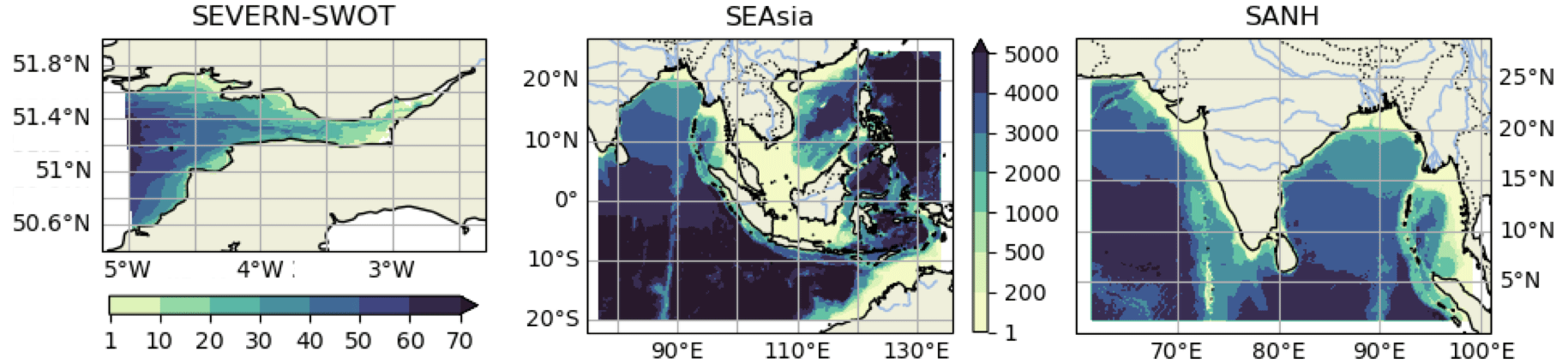
Figure 2 Bathymetry (m) from the Severn Estuary, South-East Asia and South Asia worked example configurations.

3.1 Build planning and process prioritisation

The first stage consists of planning the new configuration and how to build it sequentially. The concept is to systematically increase the complexity of the processes represented with the associated efficacy testing. This is done in order to verify that the simulated processes behave as expected and also to assist with error trapping should unexpected behaviours manifest. The first step, therefore, is to prioritise processes that need careful attention or that dominate the system. For example, many simulations in the South China Sea may be dominated by tides, whereas simulations in the Mediterranean or other inland seas may be dominated by winds. Alternatively, for simulations in the northern Bay of Bengal, special consideration may be required to accurately represent the freshwater input and its seasonal variation. Similarly, in the case of models of the Arctic or Antarctic shelves, special care should be paid to properly represent sea ice and ice shelf processes. In practice, these priorities cannot be set without consideration of the intended use of the model and will therefore be application-specific. However, having formulated a priority list, experiments can be designed whereby separate processes can be tested to sequentially build complexity in the target configuration. This is particularly useful in light of the fact that the choice of the numerical techniques adopted to solve the governing equations will inevitably affect the realism and accuracy of many of the physical processes explicitly resolved or parameterised by the ocean model (e.g. Haidvogel and Beckmann, 1999; Griffies et al., 2000). Not all processes are separable or easy to separate, and so a measure of pragmatism is required to get to the final configuration with a minimum of unnecessary complications.

As a guideline, a number of worked examples are set out in the associated repositories, which include adding tidal processes to configurations where the parent models did not have tides. For these simulations, proper representation of tides was considered fundamental. For this we choose to use terrain-following coordinates to better represent shallow-water processes and tidal forcing from FES2014 (Lyard et al., 2021). For the SANH and SEAsia examples, this represents a significant departure from the parent model (without tides and computed on geopotential levels), though many other aspects of the parent and child configurations are similar. Another example, SEVERN-SWOT, details the workflow for (one-way) nesting of a 500 m resolution child configuration in a macro-tidal coastal regime.

3.2 Obtain code, compile model executables and build tools

This step is to obtain the code and build the required NEMO-supported tools. This process is generic for all configurations. This step is largely software maintenance, rather than natural science, and can be largely automated once a successful workflow has been established. Official NEMO guidance can be found on the consortium web pages (https://sites.nemo-ocean.io/user-guide/setup.html, last access: 8 February 2023). As a necessary precursor to subsequent steps, we provide linked scripts and associated wiki documentation in the SEAsia repository (https://github.com/NOC-MSM/SEAsia/, last access: 8 February 2023) as a NEMO4 worked example on ARCHER2 (https://www.archer2.ac.uk, last access: 20 February 2023). From experience we note that there is no single “best way” to structure the directory tree, and flexibility should be encouraged according to the simulation or simulations required.

At this point it is worth briefly mentioning how users can implement choices in modelling frameworks, such as NEMO, since some choices are made at compilation and are therefore hard-wired into the executable. In NEMO there are two tiers of hard-wired choices. At the upper tier choices are made that activate NEMO modules, in addition to the core ocean (OCE) physics module, for example enabling ice or biogeochemistry capability (see Sect. 4). These modules are then compiled together. At the lower tier, choices are made within modules about which code blocks need to be compiled. These are set with compiler keys (e.g. https://github.com/NOC-MSM/SEAsia/blob/master/BUILD_EXE/NEMO/cpp_file.fcm, last access: 8 February 2023) and are used to activate, for example, MPI capability (key_mpp_mpi) and XIOS coupling (key_iomput) for input–output management. However, the majority of parameters that the user will edit, typically those which define details of and control the simulation (e.g. time step and duration, forcing data location, parameterisation choices and coefficients), are contained within namelist files that are read at run time. Therefore, for many applications, on completion of these compilation steps, the resulting NEMO executables and tools can be used for many configurations. The general direction of travel for NEMO is away from compiler keys to run-time configuration. Further NEMO-specific details are given in the worked examples.

3.3 Model domain and geometry

After planning the new configuration and successfully building the machinery needed to run it, the following stage is to identify the most appropriate model domain, horizontal and vertical resolutions, and discretisation schemes needed to adequately resolve the spatial scales and the processes the new configuration is targeting. The final outcome of this crucial stage is the definition of the 3D geometry of the model domain, including the horizontal and vertical coordinates and the 3D grid spacings, which typically vary for variables defined on the different faces, corners and centre points of the grid cells.

Starting from version 4.0, NEMO loads at run time an externally generated domain configuration file containing all the relevant grid geometry information. This separation of the grid-generation process from the dynamical core permits a flexible approach to grid construction. If the planned configuration is based on an existing NEMO configuration (or idealised geometries), then the work to build a new domain configuration file can be done by tools and guidance that are supplied with NEMO. However, if the proposed work is for a new regional configuration, as is the main theme of these workflows, then the guidance outlined below is indispensable for directing the process.

• Locations of boundaries. For the worked example, these are chosen with consideration of the tidal harmonics. It was verified (using TPXO9, Egbert and Erofeeva, 2002, FES2014, Lyard et al., 2021, or another tidal product) that none of the four largest semi-diurnal or four largest diurnal species had amphidromes near the proposed boundary, since for fixed relative errors in tidal amplitudes, small absolute errors at the boundary could scale to large absolute errors in the interior.

  A principle of regional ocean modelling is to nest with the parent model in the deep ocean. Ocean–shelf exchange processes are complex and fine scale and exert a first-order control on shelf seas (Huthnance, 1995), so it is expected that they would be better represented by the child model than the parent model. This choice comes with two penalties. The deeper water necessitates a shorter barotropic time step, and steep continental slopes can cause issues of horizontal pressure gradient error for terrain-following coordinate models. So, the alternative of nesting on-shelf is also preferred for some studies (e.g. Holt and Proctor, 2008).

• Boundary bathymetry. In a regional model, the boundary interface with the parent model is a likely source of instability, especially if the grids are different. In light of this, the boundaries can be chosen to avoid grid-scale highly irregular bathymetry near the boundary (small islands or sea mounts and steep bathymetry) and to seek near-orthogonal intersections between the boundary and the features, as done in the SEAsia configuration. An alternative is to precisely match the bathymetries at the boundary, with the child being interpolated to the target resolution and then having a halo region inside the boundary, where the bathymetry is smoothly transitioned to the target child bathymetry. However, this sophistication is not required for our examples.

• Bathymetry pre-processing. The final bathymetry will be mapped onto the target grid. For a wide-area domain this may require patching together bathymetries from separate surveys or, more likely, using a gridded product where merging has already been performed. It is worth checking the data for spatial discontinuities and applying appropriate filtering (though being cautious not to oversmooth length scales explicitly resolved at the model's resolution). Conversely, bathymetry projected onto the target resolution may adversely affect the large-scale flow (e.g. if a narrow strait becomes closed or the flow is otherwise restricted, or islands are lost). Similarly, bathymetry at the target resolution may produce instabilities (if model levels get too thin with ebbing tide) or generate spurious currents for terrain-following coordinates over steep bathymetry. In these situations user-defined modifications to the bathymetry might be necessary according to the target grid (see e.g. the SEVERN-SWOT configuration). Note that the absence of systematic recording of the steps taken for bathymetric pre-processing is an endemic problem in model reproducibility that should be avoided.

• Bathymetry reference datum. An important aspect of processing bathymetry data, for use in a numerical model, depends on the vertical reference datum in the source grid. Configurations with large tides and/or surges need to pay particular attention to the source bathymetry datum. Often the bathymetry is referenced to the lowest astronomical tide (LAT), e.g. EMODnet (Lear et al., 2020). While it is useful for chart data to be referenced to LAT for navigational purposes, the bathymetry needs to be referenced to the mean sea level (MSL) for modelling purposes. There are however fundamental limitations to the accuracy of this process since LAT is not accurately known in the absence of multi-year tidal records. Therefore the process of referencing and de-referencing the bathymetry to LAT is problematic. Nevertheless, it may be achieved to first order from a long multi-decade integration of a tide-only model of the region of interest by using the lowest obtained sea level as a proxy for LAT.

• Negative bathymetry and reference geopotential height. For configurations that involve inter-tidal zones, the bathymetry can be negative relative to MSL. To deal with negative bathymetry, NEMO can use a reference geopotential level defined at some height above MSL, so that all potentially wet points are below this reference level. Care is required when generating initial conditions and stretching of vertical coordinates to take into account the use of a non-zero reference depth.

• Critical depth for wetting and drying. In NEMO there is the option to allow for a grid cell to dry out as the tide ebbs. This is implemented in practice by limiting the fluid flux out of the cell when a user-defined minimum depth is reached. The specification of this minimum depth will be application-dependent (typically a few centimetres) and requires a compromise between maintaining numerical stability, for a given time step, against the enhanced realism of thinner critical depths (see for example the SEVERN-SWOT configuration).

• Grid discretisation. When designing the computational mesh, the lateral extent of the domain and the 3D resolution are likely to be determined by the experiment requirements and the available HPC resources. In the horizontal direction, NEMO supports structured quasi-orthogonal curvilinear quadrilateral Arakawa These types of grids can offer a goodC grids. These types of grids can offer a good degree of compromise between flexibility and accuracy, allowing one to improve the representation of many coastal processes (e.g. the propagation of Kelvin waves and land–ocean interactions through the aligning of grid lines with the coast Adcroft and Marshall, 1998; Greenberg et al., 2007; Griffiths, 2013). In addition, they can be used to refine the resolution in a specific location of the domain to improve for example shelf–open-ocean exchanges (e.g. Bruciaferri et al., 2020). However, since they rely upon analytical coordinate transformations, they typically have limited multi-scale capability in comparison to more versatile (e.g. triangular-mesh) unstructured grids (Danilov, 2013). In the vertical direction, NEMO takes advantage of quasi-Eulerian generalised vertical coordinates $s(x,y,z,t)$, where the time dependence allows model levels to “breathe” with the barotropic motion of the ocean. In domains with shallow seas and tidal dynamics, a species of terrain-following coordinates is often adopted in order to provide vertical resolution to resolve highly dynamic tidal processes on the shelf (Fig. 2) as well as being able to resolve the open-ocean forcing conditions and structured water-mass properties (see for example Wise et al., 2022). In a linked example (e.g. SEAsia) we chose 75 levels of hybrid z-sigma vertical coordinates. These were configured so that below the 39th level (at around 400 m) the coordinates would transition to the z-partial step so as to favourably compare with the parent z-partial step.

• Process-oriented experiments. It is often useful to conduct simple numerical experiments to assess whether the chosen 3D model geometry is numerically stable and accurate enough for the target application. For example, steeply sloping model levels can introduce errors into the computation of the horizontal pressure force (e.g. Mellor et al., 1998). In such a case, conducting idealised horizontal pressure gradient tests can be instructive to ensure that the chosen vertical discretisation scheme does not introduce undesirable spurious velocities (e.g. see experiment 1 of Bruciaferri et al., 2018, or Wise et al., 2022, for details on the idealised or realistic scenarios, respectively). Similarly, geopotential z coordinates can introduce excessive spurious entrainment and mixing when simulating gravity currents (e.g. Legg et al., 2006). Therefore, idealised cascading experiments similar to the ones of Wobus et al. (2013) or Bruciaferri et al. (2018) can be useful for revealing excessive dilution of dense overflows. Finally, tide-only forced experiments in barotropic (first) and stratified (after) set-ups can be extremely useful for early detection of issues in the model geometry that could negatively affect the accuracy of the simulated tidal dynamics (see experiment 3 of Wise et al., 2022, for details).

Worked examples are given for the https://doi.org/10.5281/zenodo.6423211 (Jardine et al., 2022), https://doi.org/10.5281/zenodo.6483231 (Polton et al., 2022a) and https://doi.org/10.5281/zenodo.7473198 (De Dominicis et al., 2022) domains. For these new configurations, initial tests were conducted to ensure that horizontal pressure gradient errors were acceptable and that the tides were simulated accurately. Having addressed any emergent problems with these tests, additional complexity can be sequentially added: realistic initial conditions, realistic temperature, salinity and velocity open boundaries, meteorological forcing and finally freshwater forcing.

In summary, the steps to create the domain file are to first create a set of coordinates for the target grid and then make a bathymetry for these coordinates. Finally, extend the domain in the z direction with the chosen types of vertical coordinates to complete the 3D discretisation of the domain.

Note that the domain configuration file is static with respect to time. Any time variability in, for example, the vertical grid can be captured at run time with the output files.

3.4 Initial conditions

Initial conditions can be idealised or realistic. Effective use of appropriate initial conditions can expedite the spin-up of a model in slowly evolving regions of the domain (e.g. deep-water salinity). However the initial conditions are constructed, it is likely that they are imperfect and that at least some spin-up time is required for dynamical adjustment on the child grid. For example, the default initial condition machinery in NEMO uses only temperature and salinity with the expectation that the velocity field can be spun up from rest.

An alternative is to pose a “soft-restart” state rather than initialising the model from rest. In the soft-restart method, salinity, temperature, current velocities and sea surface height from, for example, a coarser-resolution model or a reanalysis product are interpolated into the model grid and are then used to create a pseudo-restart file. Using this method requires a shorter spin-up to allow the model to adjust to any instabilities. The worked example in the SEAsia repository details how to generate a pseudo restart for a reanalysis product.

A principle is to match initial-condition and lateral-boundary-condition data (for temperature and salinity). A mismatch here can generate density-driven currents tangential to the open boundary, which may persist long into the simulation under geostrophy. The most common potential challenges can be grouped into issues arising from inconsistencies across products.

• Parent-to-child grid interpolation. The parent and child grids are likely to be different. Therefore, the coastline and bathymetric features will likely have different representations such that the child might have land points where the parent has wet points or vice versa. Flood filling prior to interpolation (lateral filling of all land points with nearest-neighbour wet-point values) and downfilling isolated canyons (using e.g. SOSIE tools (https://github.com/brodeau/sosie, last access: 27 May 2022) can address issues of bathymetric representation following interpolation. Additional smoothing of tracer fields may also be required if, for example, new straits are opened by the child grid. Furthermore, the representation of the ocean interior might be different between the two grids. For example, a pycnocline might be poorly represented between two thick levels in the parent grid, but how should this “step” be represented in a finer-resolution child with increased vertical resolution? Whatever method scheme is chosen, it is likely therefore that some spin-up will be required to let fine-scale features evolve. This spin-up should be of a similar order to the flushing time of the shelf sea basin (ranging in coastal ocean regions from several days to multiple years: Liu et al., 2019).

• Equation of state. With a non-linear equation of state, interpolating temperature and salinity onto a child grid will not ensure preservation of static stability. Alternatively, the equation of state that generated the parent data might be subtly different from the equation of state in the child model. Though these effects are likely to be small and quickly dissipate, in practice they have been seen to trigger convection in marginally stable environments. So, checking for static stability of the initial condition is recommended if stability issues arise in the first few time steps.

However the initial conditions are constructed, it is likely that they are imperfect and that at least some spin-up time is required for dynamical adjustment to the child grid to occur.

Even if the target initial conditions are prescribed as being from a “realistic” source, it can be an instructive and time-saving route to a final configuration to start with idealised initial conditions. NEMO has the facility to compile user-defined initial conditions into the executable, which can be invoked by namelist parameter choices at run time. In the supporting SEAsia repository, two examples of idealised initial conditions are used: (a) domain-constant temperature and salinity; (b) horizontally homogeneous temperature and salinity, constructed from the World Ocean Circulation Experiment (WOCE) climatology to be broadly representative of the region. The latter is used to assess the horizontal pressure gradient errors in an unforced run, thereby testing the limitations of the vertical discretisation.

3.5 Open-boundary conditions

The lateral boundaries are the points that define the horizontal extent of the model domain. Information must be specified at these points to constrain the interior solutions, effectively providing a forcing to the model. When the regional model differs from the model that was used to generate the boundary data, which typically is the case, differences between the interior solutions will emerge. An open boundary is a way to specify the external forcing while allowing phenomena produced within the interior domain to exit across the boundary without disturbance. In some sense open boundaries allow the physical domain to extend beyond the boundary of the computational domain, for example by allowing a wave to exit the domain without reflecting back into the domain.

It is important to recognise that the formulation of open-boundary conditions tends to be based on simplified physics, focusing in particular on the hyperbolic part of the dynamics. In general, these open-boundary conditions will not be perfect, and care must be taken to assess instabilities and model inaccuracies attributable to the boundary conditions. For example, a parent model that is eddy-rich may result in data that appear noisy, leading to a mismatch in dynamics at the boundary.

NEMO offers a number of namelist options to specify different open-boundary condition formulations as well as set the frequency of the supplied data. These data typically come from an external parent model with a much lower frequency (typically daily, 5-daily or even monthly for global products). There is an option to interpolate in time.

It is possible to specify “structured” open boundaries that define the northern, southern, eastern and western boundaries as well as “unstructured” open boundaries. While the former is useful in idealised set-ups, unstructured boundaries enable complex geometries defined by a supplied coordinates file. In cases where different boundaries have different requirements, it is possible to define multiple sets of unstructured open boundaries that can use different namelist options and datasets.

The namelist is organised so that boundary conditions are separated into the 2D depth mean velocities and sea surface height, the 3D depth-dependent velocities (perturbations from the depth mean) and the 3D tracer fields. Tidal harmonics can also be specified as part of the 2D fields. Following the principle of building up complexity, it is worth configuring the open boundaries for the depth mean velocities first. This can include tidal harmonic forcing.

The choice of boundary condition, for the 2D velocities, is primarily a choice of which radiation condition to use (e.g. Flather, 1976, or an Orlanski e.g. Marchesiello et al., 2001, scheme). For the 3D velocities and tracers, one can also choose to relax the child field to the external data over a buffer zone or apply a condition to the normal flux or normal gradient. For example, it is possible to apply a radiation condition to the 2D velocities, a flow relaxation scheme to the tracers and a zero gradient to the 3D velocities.

The key considerations are whether the open boundaries are affecting either stability or accuracy. Some specifics to consider include the following.

• Parent to child. The boundary data will likely be associated with bathymetry that is different from that used by the child model. This can result in differences between the parent and child in terms of transport across the boundary. It may therefore be beneficial to match the bathymetry along the boundary. Another consideration is whether to pre-process the velocities so that the transports in the child match those of the parent when regridded. Note that NEMO allows the user to provide files that contain the full velocities (2D + 3D), which it will then separate at run time.

  The boundary data will also likely be associated with a vertical grid that is different from the child vertical grid. If they have not been regridded, then NEMO provides an option to vertically interpolate onto the native grid at run time. For 3D velocities this could lead to inconsistency with interpolated tracer fields.

  Changes in grid and bathymetry may also result in sections of the boundary that are separated from a land point by thin strips of wet grid points. This may result in spurious currents and a need to mask out certain grid points.

  The boundary velocities may also need to be rotated. If the external velocities are specified as rectangular, for example, they might require rotation to be correctly oriented on a spherical grid.

  There may also be temporal differences between the child and the parent. Specifically, models can be set up to ignore leap years, which may result in the boundary data becoming out of synchronisation with the child model time.

  Finally, even if the vertical grids are the same, mismatches can occur if different types of free surfaces are applied: many regional applications use non-linear free surfaces, whereas global models often use fixed z levels. These effects are strongest in the surface layers and could be mitigated by constructing boundary conditions from volume fluxes, if appropriate.

• Tides. As previously noted, tidal amphidromes should ideally be away from the boundary. Additionally, as previously noted, a mismatch in parent–child bathymetry can result in a mismatch in transports; this also affects transports due to tides. Relatedly, it should be ensured that tides are not present in the external boundary data if tides are also specified with harmonics.

• Volume conservation. Open boundaries can allow gain and loss of water through the boundaries which may result in drift in mean sea level and accumulate dynamical errors. NEMO provides an option to maintain constant volume via a correction. For a model including tides, however, this could be considered inappropriate.

• Spurious currents. Spurious currents can be generated at open boundaries that appear trapped but that may affect the interior momentum over time. Areas where the boundary intersects the continental margin are particular areas of concern because the sloping bathymetry can act as a wave guide for spurious variability. A further consideration is the effect on non-physical aspects of the model, such as biogeochemistry (see Sect. 4.1). High vertical velocities at the boundary may not be apparent due to flow relaxation at the boundary. However, tracers that are not relaxed at the boundary will feel the effect of spurious vertical currents.

Following the above guidance to build sequentially, whereby complexity is incrementally introduced, it can be instructive to include open-boundary conditions with a sequence of developments. Our workflows lean heavily on the PyNEMO community Python tool (https://github.com/NOC-MSM/PyNEMO, last access: 4 July 2022). A tide-only example (forcing by FES2014 tides, initial temperature and salinity are set constant, velocities are initialised as zero and boundaries are set to initial values) can be found in the SEAsia and SEVERN-SWOT repositories. The documentation includes generation of the boundary conditions and running of the model. For boundary conditions including 2D and 3D velocities as well as temperature and salinity, see the SEVERN-SWOT repository. The documentation includes generation of the boundary conditions and setting of the namelist.

3.6 Atmospheric forcing

In this discussion we consider atmospheric forced ocean models and atmosphere–ocean coupled models.

3.6.1 One-way atmospheric coupling

In the one-way (forced-ocean) set-up, it can be helpful to consider that the meteorological processes can affect either the thermohaline properties (via heat and radiation fluxes or precipitation and can be applied as boundary conditions in the tracer equations) or can affect the ocean momentum (via pressure and wind speed). These atmospheric boundary layer processes must be parameterised in order to compute fluxes with which the ocean can be forced. NEMO has a number of parameterisation options (or Bulk formulations): (i) NCAR (Large and Yeager, 2004), designed for the NCAR forcing, but also appropriate for the DRAKKAR Forcing Set (DFS) (Brodeau et al., 2010); (ii) COARE3.0 (see Fairall et al., 2003); (iii) COARE3.6 (see Edson et al., 2013); (iv) ECMWF, appropriate for ERA5 data (Beljaars, 1995); (v) ANDREAS (see Andreas et al., 2015). Alternatively, if all the atmospheric fluxes are known, these can be supplied directly as surface boundary conditions.

In addition to choosing the appropriate source and type of surface boundary condition, there are a few additional considerations to be borne in mind when preparing the atmospheric forcing dataset for a target child model that has different spatial or temporal discretisations from the parent. (1) Calendar stretching (e.g. 3 h forcing on a 360 d calendar being mapped to a Gregorian calendar). (2) Land–sea masks can differ between the parent atmospheric grid and the child ocean grid. This is especially problematic when a coarse parent grid is naively interpolated onto a finer child grid. The mismatch in coastlines results in misrepresentation of near-coast heat fluxes and sea breeze dynamics but can be alleviated using flood-filling techniques whereby extrapolation and interpolation are applied separately to land points and sea points, though problems can still arise if the child grid has islands that simply do not exist in the parent grid. Finally, subtle differences in the atmospheric data expected by the bulk formulae are a common source of error (e.g. reference levels, specific versus relative humidity, net versus downward long-wave and short-wave radiation). So, as is often the case when re-purposing a complex system by modification, “trust but verify”. A worked example is given in the SEVERN-SWOT repository using ERA5 surface forcing data (data access: https://www.ecmwf.int/en/forecasts/dataset/ecmwf-reanalysis-v5, last access: 9 February 2023). The documentation includes these global data being cut down and manipulated for use in forcing a regional configuration and then running the model with one-way meteorological forcing.

3.6.2 Two-way atmospheric coupling

In regional two-way coupled atmosphere–ocean models, the information transferred to the ocean from the atmosphere is essentially very similar to that provided in a one-way forced set-up, when the fluxes are known. The solar and non-solar surface heat flux, mean sea level pressure and freshwater flux are transferred as well as the momentum fluxes from atmosphere to ocean (Lewis et al., 2019a). Then either the surface temperature, surface currents or both can be sent back to the atmosphere. The variables are exchanged between both models via a coupler such as OASIS3-MCT (Valcke et al., 2015) and interpolated between the two grids, typically using first-order conservative interpolation for scalars and bilinear interpolation for vector fields.

The coupling frequency can be optimised by considering the region over which the model is being run and the features and dynamics that dominate that area. However, it must be set to a value larger than the model time step. Wang et al. (2015) use a 3 h coupling frequency for their climate atmosphere–ocean model located over the Baltic and North seas, but Zhao and Nasuno (2020) found that a coupling frequency of hourly or sub-hourly better reproduced the sea surface temperature and consequently stronger convection during the passage of the Madden–Julian Oscillation. In the regional coupled suite RCS-IND1 (Castillo et al., 2022), an hourly coupling frequency was used to capture the temperature diurnal cycle; however, options to move to using a 10 min coupling frequency are mentioned, as this might prove beneficial for modelling rapidly changing conditions as in squalls and tropical cyclones.

There is a risk that coupled atmosphere–ocean models may become unstable and drift when run over long periods of time due to the feedbacks between both models. To constrain the drifts, nudging or weakly coupled assimilation may be required. However, not all models require corrections, the decadal-scale run carried out by Wang et al. (2015) and the 100-year simulation in Primo et al. (2019) being examples of this. Alternatively, mixed two-way and one-way forcing approaches can be applied if either coupling or direct forcing is not appropriate for the entire domain.

3.7 Terrestrial river forcing

This aspect of configuring a regional model is uniquely challenging: river flow data typically come from gauges, which are typically far upstream from the model's coastal grid point, or from hydrological models, where the data are gridded but not necessarily at fine enough resolution for the target application (e.g. many global products have a $\mathrm{1}/\mathrm{4}$^∘ resolution). Pre-processing freshwater data can be particularly time-consuming, so it is worth giving careful consideration to design choice options at the outset. Where possible, consistent atmospheric precipitation and riverine data are preferred for consistent freshwater budgets. For example, the JRA-55 (Tsujino et al., 2018) and COREv2 (Large and Yeager, 2009) datasets have an accompanying freshwater river dataset. However, while consistent forcing is desirable, a dataset with a range of consistent variables may have lower accuracy than e.g. a region-specific flow-only dataset. In some strongly forced applications, forcing accuracy in specific variables may be more important than consistency across all forcing variables. See the SANH repository for an example that generates river forcing from different sources and Sect. 4.1.3 for specific guidance on constructing riverine biogeochemical fluxes.

Having identified the data sources and the corresponding model grid points for freshwater inputs (itself a heavily labour-intensive exercise that defies straightforward automation), there are further choices to be made regarding the implementation. (i) How is the freshwater distributed horizontally? If the coastal outflow is a river delta, the freshwater load should be distributed between the tributary channels. Similarly, if the volume flux is large and baroclinic dispersal processes are not resolved, then unrealistic freshwater lenses can accumulate at the coastline. This can also be remedied by redistributing the freshwater flux across neighbouring grid cells. (ii) How is the freshwater distributed vertically? The freshwater can be vertically mixed to a specified depth or enter as a surface plume. (In our mid-latitude and tropical applications with biogeochemistry, we typically mixed the freshwater over the top 10 m for numerical stability.) Increasing vertical diffusion at river points can be used to compensate for unresolved estuarine mixing. (iii) What are the salinity and temperature of the river water? The default implementation is often to add freshwater (zero salinity) at the temperature of either the sea surface or the atmosphere; however, better results are likely if observed or river model values are used. These choices can be adjusted to achieve target temperature and salinity characteristics of the plume. To date there has been no accommodation for groundwater fluxes, though these can be considerable (Zektser and Loaiciga, 1993). Finally, validation to ensure accurate estuary-mouth forcing is challenging. Satellite salinity has a resolution of approximately 35–50 km for the Soil Moisture and Ocean Salinity (SMO) and 100–150 km for the Aquarius satellites, whereas in situ measurements capture plume features (and freshwater intensifications) at scales O(10 m) that are much finer than the resolved scale but that lack spatial coverage. Where possible, use should be made of near-coastal buoy and survey data, but in the absence of this we must settle for far-field validation against hydrography, accepting that this conflates the effects of circulation and surface forcing.

The worked example in the SEAsia repository details how rivers fluxes were taken from the JRA-55 dataset (Tsujino et al., 2018) and mapped to the nearest coastal grid point. Subtleties for large rivers include (i) avoiding placement of domain boundaries near large river outflows and (ii) laterally spreading the coastal source points to represent deltas and also to avoid unrealistic numerical issues if outflow values are locally too large.

3.8 High-performance computing: decomposition and optimisation

Modelling frameworks like NEMO are equipped to be run on high-performance computing machines. This is facilitated by the optional abstraction of input–output procedures (XIOS) from the dynamical model (NEMO). These can then be separately optimised for the target machine and, crucially, most I/O to disk can be overlapped with the continuing computational tasks. Most HPC platforms will have multiple nodes, each comprising a number of CPU cores and some shared memory. However, NEMO and XIOS have different computation and memory requirements. Making the best use of each HPC platform can be further complicated by the service's charging algorithm and possible non-linearities in performance scaling arising from subtleties in hardware design. Nevertheless, when configuring a simulation, there are only two sets of fundamental considerations.

1. How many compute cores will be allocated to the dynamical core and how many cores should be assigned to each node? Each core will have a roughly equal grid cell fraction of the surface map of the whole domain (parallelised sub-domains contain the full water column).

2. How many cores should be dedicated to the XIOS processes, and how many cores should be assigned to each node?

Some general guidance can be offered to address these questions.

• Computational resource splitting. The best ratio of XIOS to NEMO cores depends on the volume of data to be written. Since this is configurable at run time via the XML files, some care is needed to provide the XIOS processes with sufficient resources to cope with any expected variations. Though there are no easy answers as to how to optimise domain decomposition, a starting point would be to allocate cores between NEMO and XIOS in a ratio of $n:\sqrt{n}$. Often, fewer XIOS cores are required, but each XIOS process is likely to require access to more memory than each ocean core. Typically, this is achieved by running XIOS cores sparsely populated on dedicated XIOS nodes or by using options to control placement of processes to CPUs on nodes running a mix of XIOS and ocean cores. The best solution will be hardware-specific. For example, in a system with four NUMA regions per node, you may choose to place one XIOS process alone in the first NUMA region (thereby giving it access to the maximum amount of shared memory) and to fully populate the remaining NUMAs with ocean processes. Performance optimisation of the NEMO-to-XIOS decomposition comes with experimentation. Timing information provided in the timing.output file (generated when ln_timing = .true.) can be used to decide on the number of ocean cores by checking the average time per time-step figure for a variety of decompositions. Optimising the number of XIOS cores is usually more a case of finding the minimum number that will cope with the demands determined by the XML files. Insufficient XIOS resources may simply mean a longer-than-necessary wait at the end of a run, but it can also lead to intermittent “out-of-memory” failures when disk I/O fails to keep up with the requests entering the queue. XIOS will report performance statistics at the end of a successful run.

• Domain decomposition. It is good practice to allow NEMO to automatically define the domain decomposition. This happens when np_jpni and np_jpnj are <1. The model will take the number of ocean cores provided to the parallel run command (e.g. mpirun) and will minimise the horizontal sub-domain size and maximise the number of eliminated land-only sub-domains. It is likely that your first guess at the ideal number of ocean domains is not optimal; pay attention to messages in ocean.output for advice on better choices. See Sect. 7.3 of the NEMOv4.2 reference manual for more details. Experiment with a range of decompositions and use considerations of cost and “time to solution” to decide on your best choice. As a rule of thumb, it is likely that performance will not scale with domains smaller than around 7×7 points since communication will begin to dominate over computation with domains smaller than this. However, this is only a guide, and NEMO developments towards exascale computing are continuing to challenge these limits. In older versions of NEMO, land suppression (to avoid computation over land points) had to be explicitly activated (e.g. the SEVERN-SWOT unforced run example). This efficiency saving has automatically been activated since NEMOv4.2.

3.9 Troubleshooting

Invariably, during the course of developing a new configuration, a number of problems will be encountered where the model blows up or otherwise does not behave as expected. The general principle for more rapidly building a new configuration is to make changes slowly. In that, we mean starting from something that works and sequentially testing incremental changes rather than making multiple changes at once.

The most common problems new users encounter fall into two main categories: (1) compilation and start-up difficulties and (2) run-time stability issues or, equivalently, “getting past the first time step” and “getting beyond the first few inertial periods”. Often, difficulties in the first category arise from inconsistencies in the build environment. It is essential, for example, to compile XIOS and NEMO executables in identical machine environments, and this must include netCDF4 libraries which have been compiled with full parallel support if all the functionality of XIOS is to be used. This same environment must then be used at run time. It is always a good idea to test the environment and batch system with one or more of the NEMO reference configurations before tackling your own, custom, configurations. This will separate system issues from any issues introduced by your own changes. One way to do this is to run all or parts of the SETTE testing suite. There is a full section in the NEMO user guide (https://sites.nemo-ocean.io/user-guide/sette.html, last access: 8 February 2023) explaining how to do this. At a minimum, it is recommended to run the GYRE_PISCES configuration which requires no external data files.

After this, any continuing start-up issues with custom configurations should be isolated to the user's code changes, errors in the input files (including namelists) or resource size issues (e.g. your model requires more memory than is available on the nodes you are assigning). Precise advice will be machine-specific and depends on how the architecture is configured, but both XIOS and NEMO will detect and report many issues. Check both the batch output logs and the ocean.output file(s) for messages. Use the Discourse (https://nemo-ocean.discourse.group, last access: 9 February 2023) message channels for community support in interpreting any failure whose cause is unclear. If failures are sudden, unlocated in the code and catastrophic, then recompile NEMO with compiler debug flags (at a bare minimum employing the -O0 -g flags) and try to obtain a traceback, which identifies where in the code the crash has occurred.

Once past the first time step, the next failures are usually due to numerical stability issues or I/O issues at a future checkpoint. Even the best-prepared initial conditions are likely to trigger fast-moving responses (e.g. coastal trapped Kelvin waves) at start-up. Often, any numerical stability issues associated with this initial adjustment can be avoided by running a short period with a reduced time step. A more general section on model stability constraints is included below. I/O issues at a future checkpoint will either be errors in the input files (e.g. the model reaches a point when it requires the next month's surface forcing, but those files are not available) or output issues associated with specific output. Examples of the latter include XIOS/netCDF4 detecting “not representable” values (usually a good indication that NaNs are occurring in the simulation) or memory limits being reached due to a sudden surge in output requests. If the latter occurs in an established simulation with no new demands on XIOS, then it may be indicative of external influences changing the usual rate of I/O to disk (faulty switches, etc.).

Here we touch on some general issues that can arise.

Syntax errors in XIOS

The XML files which control the XIOS output are very sensitive and susceptible to syntax errors. Commonly, syntax errors in the XML files manifest in a lack of output or a model failure when writing output. To avoid these difficult-to-trace issues, it is strongly recommended that you edit the XML files independently of other changes being introduced to a working configuration and test each change in short test simulations.

Model stability constraints

As with most explicitly formulated computational fluid dynamics codes, it is critical that the time step is shorter than the time it takes for a substance to cross a grid box, so that the flow of mass, tracer or the propagation of waves are resolved. In configurations with deep water and a free surface, the shallow-water wave speed will likely be the time-step-limiting process. Accordingly, the time step will linearly decrease with refinement to the horizontal resolution. This can make a fine-scale coastal model with some deep-water grid points computationally expensive.

Similarly, horizontal diffusion operators limit the time step, though here it is the square of the grid spacing (Δx) that limits the time step (Δt). For example, a Laplacian diffusion operator would scale $\mathrm{\Delta }t<\mathrm{\Delta }{x}^{\mathrm{2}}/K_{\mathrm{lap}}$. So, a factor of 2 reduction in grid spacing would correspond to a factor of 4 reduction in the time step. This can be offset by a linear reduction in the diffusion coefficient K_lap (units m² s⁻¹ and represented as a velocity scale multiplied by a length scale). Similar analysis can be performed for bi-Laplacian diffusion (with coefficient K_bi, units m⁴ s⁻¹) such that $\mathrm{\Delta }t<\mathrm{\Delta }{x}^{\mathrm{4}}/\mathrm{|}{K}_{\mathrm{bi}}\mathrm{|}$. There are many other more subtle and nuanced stability constraints relating to most areas of the dynamics: understanding these generally requires detailed numerical analysis, and so they are usually left to trial and error. Nevertheless, the process can be facilitated by inspection of Courant–Friedrichs–Lewy (CFL) diagnostics (for example, activated through the namelist parameter ln_diacfl) and noting that in shallow tidally active regions the CFL criteria can also be violated by vertical velocities.

Code errors

Despite one's best endeavours, the code base can have errors (especially, for example, on branches that are being actively developed). Also, user implementation errors (e.g. inappropriate coefficients, as discussed above) can be hard to distinguish from parameterisation failures, which can both typically have explanations that are attributable to physical characteristics of the domain (e.g. the simulation blows up in a strait/over a sea mount/at a coastal inlet/on a spring tide/following intense stratification events). On the other hand, code errors arising from incorrect indices or variables may appear to have a more random behaviour (e.g. crash point moves with a changing number of cores or otherwise “surprising” or non-Newtonian behaviour).

With any advanced technology, troubleshooting is an inevitable part of developing. Therefore, document your work; revert to a last working set-up (if it exists) when things do not go as expected. Finally, making sure your issues are reproducible will help if you seek assistance.

4 Additional modules

One of the strengths of the NEMO framework is the broad community user base that actively develops additional modules that augment and enhance the value of the physics-only ocean simulations. In the following, experiences are shared relating to biogeochemical, wave and ice modelling.

4.1 Biogeochemistry

A significant challenge of regional biogeochemical modelling is in initialising all the necessary fields and supplying appropriate surface and lateral boundary conditions along with river inputs. This is complicated by the fact that data for initialising and forcing biogeochemistry models can come from a variety of sources and usually require some pre-processing before it can be applied. In particular, special attention should be paid to the data units, which might need to be converted according to the model-specific requirements. Specifically, concentrations should not be confused with fluxes.

A number of data sources are publicly available, both observational and modelled. Widely used observational global products include the World Ocean Atlas (Boyer et al., 2018b, https://www.ncei.noaa.gov/products/world-ocean-atlas, last access: 9 February 2023), containing monthly gridded inorganic nutrients and dissolved oxygen in the upper 800 m and annual values deeper, and GLODAP (Olsen et al., 2016, https://www.glodap.info, last access: 9 February 2023), containing annual gridded dissolved inorganic carbon and total alkalinity as well as inorganic nutrients and dissolved oxygen. Modelled products, such as CMS global models, using PISCES, contain simulated nutrients and phytoplankton fields. For regionally specific products, data may be available from regional consortia and programmes (e.g. North Sea Biogeochemical Climatology, NSBC (Hinrichs et al., 2017, https://www.cen.uni-hamburg.de/en/icdc/data/ocean/nsbc.html, last access: 9 February 2023), and the EMODnet portal Lear et al., 2020, https://emodnet.ec.europa.eu/en, last access: 9 February 2023). However, observational sources include a limited number of measured parameters, while modelled data are likely to be generated by a model with a different (usually simplified) trophic structure compared to the target biogeochemical model. Assumptions will therefore have to be made when generating initial and boundary conditions to infer the required fields based on the available data; application of the Redfield ratio can be a valuable tool to preserve the stoichiometry when deriving the relative elemental composition of living organisms. Ideally, physics and biogeochemistry boundary and initial conditions would come from the same source. When using data from different sources, care must also be taken to avoid or manage potential mismatch issues between, for example, the depths of the nutricline and the pycnocline. In these circumstances one would expect the simulations to require a spin-up period. The length of spin-up will depend on various aspects of the region's dynamics and the quality of the starting conditions of the key state variables. For example, a timescale of several months is typically sufficient for most pelagic variables, whilst certain benthic variables can take several years or even decades to reach equilibrium. As with physics-only regional models, attention needs to be applied to appropriately formulating the model forcings and inputs. Generalised considerations when initialising a biogeochemistry simulation are presented in the following sub-sections.

4.1.1 Initial conditions

It is generally preferable to initialise the biogeochemistry in low biological productivity periods. This reduces model uncertainty as the phytoplankton and zooplankton are at their lowest values and nutrients are mainly present in their inorganic form. In the absence of appropriate data, distributions of phytoplankton functional groups can be estimated from measured chlorophyll. Other pelagic variables for which detailed data are not available (e.g. concentrations of dissolved organic carbon, calcite and bacteria) are typically initialised to constant values, ideally derived from any available observational data in the region. Distributions of benthic variables are often difficult to estimate as there are usually few data available. Climatological profiles can be used but may not be representative of the target region of interest. It can take years, even decades, for some components (such as organic matter and macrofauna) to adjust. Our experience suggests that underestimated organic matter content will increase more quickly in shallower, productive areas than overestimated content takes to decrease in deeper regions.

4.1.2 Surface boundary conditions

The biogeochemical fields required for surface boundary forcing will depend on the region of interest and the target application. By way of example, nitrogen deposition is an important source of nutrients to the system and is commonly prescribed. Model products (e.g. EMEP for Europe, HTAP for Global Simpson et al., 2012; Tan et al., 2018) are a useful data source. In shallow-water regions light attenuation due to coloured dissolved organic matter (Gelbstoff absorption) can affect the radiation budget (e.g. Kara et al., 2005). It can be prescribed using data from ocean colour observations such as those provided by OC-CCI (Sathyendranath et al., 2019). Atmospheric pCO₂ data should be provided for any model that includes a carbonate system. Observational data can be converted from the fCO₂ product available through SOCAT, the Surface Ocean CO₂ Atlas (Bakker et al., 2016). In some areas iron deposition may be important and can be included through modelled products such as provided by the framework of the United Nations Joint Group of Experts on the Scientific Aspects of Marine Environmental Protection (GESAMP) model ensemble (Myriokefalitakis et al., 2018). Though it is important to note that since only a small fraction of iron dust that lands on the ocean surface becomes bioavailable, any surface boundary values should be adjusted accordingly.

4.1.3 River input

Observational data are (usually) the most precise source of data but are limited in availability. In general, it is better to use the same source for all rivers included in the model set-up. Therefore, modelled products such as GlobalNEWS (Mayorga et al., 2010) and HYPE (Arheimer et al., 2020) can be the best options, though they will require, or implicitly make, some assumptions regarding land use. In some cases excessive anoxic conditions can form around river mouths, typically with larger rivers in regions already subject to anoxia. Therefore, if riverine oxygen is needed but is unavailable, impose a concentration around the saturation value. Any data on river inputs will usually contain a limited number of variables compared to requirements of the target model. Therefore, assumptions will have to be made, for example partitioning total nitrogen inputs into various inorganic and organic fractions. A worked example generating river forcing (discharge and nutrients) from the GlobalNEWS2 model is given in the supporting SANH and Partridge (2022b) repositories.

4.1.4 Lateral boundary conditions

Lateral boundary condition forcing data should be obtained similarly to the initial condition data. Typically a flow relaxation scheme (FRS) is used as a boundary condition for fields where values are available, which usually include inorganic nutrients, DIC, total alkalinity and dissolved oxygen. Other variables are conserved within the domain by using a zero-flux (Neumann) condition. However, this can fuel spurious behaviour around the boundaries (e.g. non-depleting high levels of nutrients at the boundary can lead to phytoplankton blooms in the region nearby). This can be mitigated by setting low boundary values for phytoplankton. Long-living material, such as organic semi-labile and semi-refractory organic matter, can propagate into the domain over decadal simulations if applied at unrealistic levels. Particular care on the treatment of depth-varying velocities at the boundaries is required when including biogeochemistry in the configuration. Unconstrained tracers at the boundary are susceptible to instabilities from erroneous vertical velocities, which would not be seen in constrained tracers, and hence are not apparent in the physics-only simulation with boundary-constrained temperature and salinity.

4.1.5 Output testing

Before committing to production simulations, a prudent initial test can confirm that the simulation conserves the mass of a tracer and that the boundary conditions are correctly applied. To this end we suggest the following procedure.

Create two passive tracers (TRC1, TRC2) with a uniform initial value (e.g. 1.0). Using Neumann boundary conditions for TRC1 confirms that the tracer is conserved. Using an FRS boundary condition for TRC2, with a low constant boundary value (e.g. 1E−10), confirms that the low values are not confined to the boundary after 10 time steps.

When changing machine or domain decomposition, it is advisable to check for bit-identical solutions in test simulations. Finally, be vigilant for negative or unrealistic values in areas that typically could cause problems. Such regions include boundaries, river mouths or coastlines that might “trap” and accumulate tracers.

4.1.6 Biogeochemical models used in regional configurations

Here we highlight just three biogeochemical models with which we have experience and that span a range of complexities in biogeochemical process representation.

European Regional Seas Ecosystem Model (ERSEM)-specific considerations

ERSEM (Butenschön et al., 2016, https://github.com/pmlmodelling/ersem, last access: 9 February 2023) was originally designed as a marine biogeochemistry and lower-trophic-level model for the temperate European shelf seas (Baretta et al., 1995; Wakelin et al., 2020). However, it has found application in global settings (de Mora et al., 2016) as well as in regional configurations in the other parts of the world ocean using a variety of hydrodynamic models, e.g. in the Mediterranean (Kay et al., 2020), Arabian (Sankar et al., 2018), and East China (Ge et al., 2020) seas.

ERSEM describes the biogeochemical cycling of carbon, major macronutrients (N, P, Si) and, optionally, iron. One of the distinct features of this model is that the carbon-to-nutrient ratios of functional groups are not fixed, varying depending on the environmental conditions. It also includes a carbonate system and a detailed description of the microbial food web. The standard ERSEM configuration includes 52 pelagic tracers and 36 benthic variables. ERSEM's detailed benthic module is relatively unique to biogeochemical models; however, if the appropriate initial conditions are not available, this can require an extended spin-up time. Within ERSEM, the units of carbon are specified in milligrams, whilst the other nutrients are specified in moles. Care should therefore be taken when applying e.g. the Redfield ratio to ensure state variables are presented in the correct units.

ERSEM adopts the modular and scalable structure of the Framework for Aquatic Biogeochemical Models (FABM: https://github.com/fabm-model/fabm, last access: 9 February 2023). In NEMO the coupling happens within the TOP_SRC routines via the FABM driver, with the necessary steps and changes being documented in the wiki of the NEMO4.0-FABM repository (https://github.com/pmlmodelling/NEMO4.0-FABM/wiki, last access: 9 February 2023). Worked examples for setting up ERSEM for the SANH and SEAsia domains are given in the linked repositories (SANH-BGCsetup: https://github.com/dalepartridge/SANH_BGCsetup, last access: 8 February 2023; SEAsia-BGCsetup: https://github.com/dalepartridge/ACCORD_SEAsia_BGCsetup, last access: 8 February 2023).

Pelagic Interaction Scheme for Carbon and Ecosystem Studies (PISCES)-specific considerations

PISCES is a biogeochemical model which simulates the lower trophic levels of marine ecosystems (phytoplankton, microzooplankton and mesozooplankton) and the biogeochemical cycles of carbon and the main nutrients (P, N, Fe, and Si) (Aumont et al., 2015). It is the default biogeochemistry module for NEMO and is distributed with the code base. PISCES also ships with the CROCO (Coastal and Regional Ocean COmmunity) model (https://www.croco-ocean.org, last access: 9 February 2023), which is based on ROMS AGRIF. PISCES is designed for regional and global applications. It has 24 tracers, including two phytoplankton compartments (diatoms and nanophytoplankton), two zooplankton size classes (microzooplankton and mesozooplankton) and a description of the carbonate chemistry. Optional parameterisations can be activated to control the complexity of iron chemistry or the description of particulate organic materials.

Examples where PISCES has been used to study specific regions include the Peru upwelling (Echevin et al., 2020), the Indian Ocean (Resplandy et al., 2012) and the Mediterranean (Richon et al., 2018). The PISCES community (https://www.pisces-community.org, last access: 8 February 2023) offers training materials that are suitable for beginner and advanced users.

To explore a NEMO-PISCES configuration, a 1D worked example (https://doi.org/10.5281/zenodo.7139521, Éthé et al., 2022) is given in the form of a demonstrator targeted at beginners. The demonstrator gives an introduction to PISCES and describes the steps to install and run the code for the BATS station (which can easily be changed) along with a description of the expected outputs.

Model of Ecosystem Dynamics nutrient Utilisation, Sequestration and Acidification (MEDUSA)-specific considerations

MEDUSA (Yool et al., 2011, https://code.metoffice.gov.uk/trac/medusa, last access: 9 February 2023 – requires a Met Office science repository account) was originally developed as an “intermediate-complexity” marine biogeochemistry model for global-scale, high-resolution applications (e.g. Popova et al., 2010). Its design is intended to be intermediate between simple nutrient–phytoplankton–zooplankton–detritus (NPZD) models (e.g. LOBSTER; Lévy et al., 2005) and more sophisticated plankton-functional-type (PFT) models (e.g. ERSEM; Butenschön et al., 2016). It represents the biogeochemical cycles of nitrogen, silicon, iron, carbon, alkalinity and oxygen (Yool et al., 2013). MEDUSA has 15 pelagic passive tracers and static 3D fields of carbonate chemistry and includes a simple “bucket scheme” for 2D benthic reservoirs. In NEMO the coupling happens within the TOP_SRC routines. For many applications, MEDUSA and PISCES are broadly similar but are developed by different communities and thereby offer a level of model diversity.

Since MEDUSA is a reduced-complexity biogeochemistry model, all the variables for the lateral boundary conditions can be supplied by parent data. This means that the boundary conditions can be simplified by specifying a relaxation condition on all the (physics and biogeochemistry) variables. MEDUSA coupling with NEMO is effectively one way, so, for example, phytoplankton blooms will not affect the absorption of shortwave radiation and influence upper-ocean temperatures.

Though MEDUSA was conceived as an efficient biogeochemistry model for global applications in NEMO, it has also been used in a regional configuration. A worked example for setting up NEMO-MEDUSA in a western Indian Ocean domain is given in the linked repository (https://github.com/NOC-MSM/Regional-NEMO-Medusa/, last access: 9 February 2023).

4.2 Waves

Surface wave processes mediate the transfer of energy and momentum between the atmosphere and the ocean. They are associated with surface-intensified fluxes of momentum and energy that give rise to a Stokes drift (Stokes, 1847), which makes them an essential component when modelling particle drift. Waves can also modify sub-grid-scale mixing (e.g. by injecting turbulence into the surface layers through waves breaking, Craig and Banner, 1994, or changing the character of the turbulence to Langmuir turbulence, Belcher et al., 2012); they can affect the horizontal momentum in the Ekman layer through the interaction with planetary rotation (Hasselmann, 1970; Polton et al., 2005). In near-coastal scenarios waves can give up their energy and momentum accelerating a mean flow or inducing a “wave setup” (a change in the background sea level) and can exert forces on the bathymetry, known as “radiation stress” (Longuet-Higgins and Stewart, 1964). Studies demonstrate value in coupling waves in regional operational systems, for example in drift simulation (Bruciaferri et al., 2021) but also in modifying surface temperatures by changing the depths to which the warm surface waters are mixed (Lewis et al., 2019b). Coupling also impacts the momentum transfer at the air–sea interface via alteration in surface roughness and stress, which affects the wave growths (Valiente et al., 2021).

When adding waves to a regional ocean set-up, a number of considerations need to be borne in mind when designing the configuration for the target application.

Spectral wave models are relatively expensive to run. Though spatially only 2D, the spectra have frequency and directional discretisation (and a different time step), which typically doubles the cost of the ocean-only component (e.g. Lewis et al., 2019a, and Hashemi et al., 2015).

This cost can be mitigated by the level of coupling used: if the waves and the ocean do not significantly affect each other, then the components can be run independently, or if adequate products exist and the ocean component does not significantly affect the waves, then data could be downloaded from e.g. the CMS catalogue. Cost can also be mitigated in coupled ocean–wave configurations by decreasing the rate at which variables are exchanged between modules.

Having determined whether or not the wave field needs to be simulated, the level of coupling can then be chosen. There are three “zones” where coupling can be implemented.

• 1.

  At the air–sea interface,

  • a.

    waves act as a buffer to momentum exchange between the atmosphere and the ocean, for example reducing the surface stress experienced by the ocean when waves are growing. Typically this coupling is modelled one way with a modification of water-side surface stress in the ocean module by wave growth and dissipation.

  • b.

    The presence of waves facilitates the transfer of momentum into the ocean. This can be captured by a wave-height-dependent ocean surface roughness in the ocean module.

  • c.

    Breaking waves inject turbulence into the upper ocean. This can be captured through modification of surface sub-grid-scale turbulent kinetic energy in the ocean module.

  • d.

    Feedback on the atmosphere. Coupling waves impacts the sea surface roughness and consequently affects wind speed (Gentile et al., 2021), which in turn can alter the sea surface temperature.

• 2.

  In the water column,

  • a.

    though surface intensified, the Stokes drift has a deeply penetrating effect throughout the Ekman layer via its interaction with the Coriolis force. This Stokes–Coriolis term can be added as an additional force in ocean module momentum equations.

  • b.

    Langmuir turbulence. This can be captured by analogy to convection through an additional turbulent kinetic energy production term that scales with the sizes of the cells (Axell, 2002). Though this scheme exists in NEMO, Breivik et al. (2015) note that the mechanism is structurally different from that involving the vertical shear in the Stokes drift velocity (McWilliams et al., 1997; Polton and Belcher, 2007; Grant and Belcher, 2009) and so will have different effects on the ocean surface boundary layer.

• 3.

  At the bed,

  • a.

    in water much shallower than the wavelength, the wave field is modified through an interaction with the bathymetry whereby the waves exert a (radiation) stress on the bed. This bottom stress can be added to the ocean module's momentum equations and/or wave evolution in the wave module's equations. This will often require revisiting the ocean model's bottom friction parameters if these have been tuned in the absence of explicit wave fields.

There are choices of wave models to consider. Three state-of-the-art models are widely used: WAM (WAveModel: Komen et al., 1996), WW3 (WAVEWATCHIII: Tolman et al., 2002) and SWAN (Simulating WAves Nearshore: Booij et al., 1999). They are all spectral models. Though WAM and WW3 were originally designed as deep-water wave models, while SWAN was specifically built for near-shore applications, they all now have capability in near-shore regions (see Cavaleri et al., 2018, for a comparative review).

As an example exploring first-order interactions between the wave and ocean model in a 1.5 km-resolution wide-area configuration of the North-West European Shelf, the following modifications were made: 1a, 1b and 2b. Code modifications to couple WaveWatchIII to NEMO using the OASIS coupler are reported in Lewis et al. (2019a), with associated linked repositories (https://code.metoffice.gov.uk/trac/utils/browser/ukeputils/trunk/gmd-2018, last access: 9 February 2023 – this requires a Met Office science repository account).

4.3 Ice processes

For regional modelling at high latitudes, additional processes to represent ice are required. These include

• i.

  sea ice (frozen sea water), which is prevalent at winter high latitudes and undergoes significant yearly cycling in horizontal extent and contribution to the planetary albedo,

• ii.

  ice shelves (floating bodies of ice attached to grounded ice sheets), which regulate the flow of grounded ice towards the ocean, in turn modulating sea level rise (Scambos et al., 2004; Joughin et al., 2010) and the formation of Antarctic Bottom Water (Lewis and Perkin, 1986; Foldvik et al., 1985), and

• iii.

  icebergs (calved ice sheets), which melt and represent an important component of ice sheet mass balance and the marine stratification.

4.3.1 Sea ice (SI3)

Sea ice is represented using the Sea Ice modelling Integrated Initiative (SI3) module. SI3 is a European collaboration to pool resources and develop a unified NEMO sea ice model for regional and global applications. This module specifically targets ice dynamics, thermodynamics, brine inclusions and sub-grid-scale thickness variations and is designed for an effective resolution of 10 km or coarser. SI3 is designed in close harmony with NEMO and ships with the NEMO code base.

Three data categories are required: ice thickness, snow thickness and ice fraction (or ice “concentration”). These are, of course, also required for the initial conditions.

Sea ice at the boundaries depends on whether the ice flows into the regional domain or towards the outside. If the flow is strictly outward, then the ice at the boundary takes the characteristics of the closest grid point inside of the domain. If the flow is inward, then boundary conditions are read from a BDY file.

Boundary data can be obtained from global simulations or reanalyses. Only three fields are required: ice fraction and ice and snow thicknesses. Additional fields can be provided for better accuracy: ice and snow temperature, surface temperature, ice salinity and melt pond concentration and thickness. If not provided, these optional fields are set to constant values determined in the namelist. The treatment of temperature is a bit more subtle. For instance, ice and snow temperatures are derived from the surface temperature if the latter is the only field provided.

On integration, the boundary fields can be set to the initial field or be allowed to vary if the data exist. Only the FRS boundary condition scheme is implemented for the tracer fields, but you can use “None” if there is no sea ice at the boundary.

At resolutions of order 10 km and coarser, the continuum sea ice model (like SI3) assumes that a grid cell contains representative samples of different ice floes and features. At finer resolutions this assumption is weakened, and though numerically stable, the solutions at the grid scale could be less realistic.

4.3.2 Ice shelves and cavities

Ice shelves, their cavities and the interactions with the ocean can be represented with a range of configuration design options. Important processes to be considered at the design stage include (i) the role of basal melt from the underside of the shelf on the ocean and whether this freshwater source needs to be resolved or whether it can be specified (coming from observations or another model), (ii) circulation under the cavity and whether this needs to be resolved in order to improve water-mass properties (Mathiot et al., 2017), tidal processes or melt rates and (iii) evolution of cavity geometry and whether the ice sheet and cavity geometry need to evolve with time (e.g. Smith et al., 2021). These considerations influence the implementation complexity and potentially the model stability.

In particular, we focus on the representation of the ice shelf cavities, which can be open (and explicitly represented) or closed (and therefore parameterised).

If the cavity is closed, an ice melt flux can be specified. Values can be sourced from an observational study (such as Rignot et al., 2013; Depoorter et al., 2013; Adusumilli et al., 2020) or from an ice shelf simulation. Ideally, the basal melt flux is distributed from the base of the floating ice shelf to the grounding bathymetry. This depth range can be extracted from an ice shelf draft dataset (e.g. BedMachine Morlighem et al., 2020). A current limitation of the ice shelf module is that one can only specify a constant melt flux.

If, on the other hand, the cavity is open, melt rates are computed explicitly by interaction with the circulating flow. However, unrealistic melt rates can rapidly degrade the realism of a simulation. To avoid this, pay attention to the initial conditions, the temperature and salinity biases on the continental shelf and the ice shelf module parameter settings.

To minimise noisy melt rate behaviour in a z-coordinate configuration, the near-under-ice temperature and salinity values are averaged over a specified boundary layer thickness. Alternatively, adopting under-ice terrain-following coordinates could help alleviate instabilities by explicitly resolving the turbulent boundary layer.

For open cavities, instead of interactively determining the melt, an option to prescribe the ice shelf basal melt in the cavities is also available. However, it worth noting that the melt rates need to be compatible with the circulation patterns in order to prevent unrealistic temperature and salinity values (as there is no feedback from the water temperature to the melt rate). To build this melt rate forcing, the easiest way is to run first with interactive melt in the cavity and to extract the melt rate pattern as your ice shelf melt forcing. Configuration options are flexible. If instabilities cannot be avoided in certain cavities, then a mix of explicit and parameterised ice shelves can be employed. Finally, care must also be taken when setting the minimum water column thickness within the cavity. To be stable, the initial water column thickness needs to be larger than the minimum sea surface height possible (i.e. the maximal tidal range, if tides are activated, plus the magnitude of the climatological sea surface height).

4.3.3 Icebergs

In NEMO, icebergs can be represented in two different ways: by using a Lagrangian model (Marsh et al., 2015) or by a climatology (Merino et al., 2016).

Iceberg climatology

An iceberg climatology is easy to use and applicable for any regional configuration. It simply consists of a file that describes the iceberg melt for every model point. Usually, such a file is built by extracting climatological, seasonal or interannual outputs from a global simulation that uses a Lagrangian iceberg model such as GO6 (Storkey et al., 2018).

Lagrangian iceberg model

Lagrangian icebergs are not compatible with regional configurations in general because they are not allowed to enter/exit across the boundaries. This being said, Lagrangian icebergs can be relevant for configurations that cover a large enough area that leads to complete melt of the icebergs before reaching the edge of the domain (e.g. a circum-Antarctic simulation). In order to force the Lagrangian iceberg model, the only forcing needed is a map of calving rates in cubic kilometres of ice per year (ice density being fixed in the model namelist). To build this map, you need integrated calving rates per ice shelf as provided by Rignot et al. (2013), for example, plus a pattern for calving. Multiple solutions are possible to inform the spatial map of calving: all at one point per ice shelf; randomly distributed along the ice shelf front; using output from an ice sheet model. A tool to distribute icebergs randomly is available as part of the NEMO CDFTOOLS toolbox (https://github.com/meom-group/CDFTOOLS, last access: 9 February 2023). Finally, the user can easily define the number of categories, the size of each iceberg category and how to distribute the calved mass across the category in the model namelist. Sensitivities of results to these choices are described in Stern et al. (2016). In addition to this, it is worth keeping in mind the two major limitations of the Lagrangian iceberg model in the current NEMO version: icebergs are “virtual”, and therefore they cannot serve as anchor points for land-fast ice (Li et al., 2020), and there is no fragmentation scheme, so the very large tabular icebergs do not break up and thus have too long a lifetime (England et al., 2020).

4.3.4 Ice process demonstrator

To explore a NEMO configuration with a mix of parameterised and explicit ice shelves, tides, sea ice and an iceberg climatology, a Weddell Sea worked example (https://doi.org/10.5281/zenodo.6817000, Mathiot and Hutchinson, 2022) is given in the form of a demonstrator. This is adapted from the WED025 configuration of Bull et al. (2021). The “expected results” section illustrates the melt rate and barotropic streamfunction under the Filchner–Ronne Ice Shelf in a $\mathrm{1}/\mathrm{4}{}^{\circ }$ simulation. In this demonstrator the iceberg melt climatology is specified as an additional runoff source. There is no demonstrator for the Lagrangian iceberg module. As a reference, please see the description of the global GO6 simulation set-up (Storkey et al., 2018).

5 Discussion and conclusions

Following decades of groundwork development and HPC evolution, complex-system regional ocean modelling is in the ascendancy. The paper has two parts. In the first part the principles set out here are emergent from the current working practices and are set out in order to make the current level of endeavour sustainable. There are three main challenges: (1) computational oceanography is increasingly looking towards computer science to advance its capability on diverse computer architectures (Porter et al., 2018), yet the mental bandwidth of an individual human is approximately constant. (2) Ocean configurations are increasingly complex and hard to reproduce. (3) The research community does not have a mechanism or is not used to valuing technical outputs that are contributions to the community.

We advocate a stronger implementation of reproducible practices and make the case that, through systematic workflows and standardised assessments, skills can be democratised, debugging can be accelerated and, in general, more time can be directed to scientific questions. Containerisation could be a means to achieve some of these goals.

In this paper we have made a distinction between making a configuration reproducible (by e.g. a machine) and making the workflow for generating a new configuration reproducible by a machine. This is because, in our scientific applications, we invariably are pushing frontiers in some aspect of the configuration-building process, e.g. with new process representation, grid structure or machine architecture. So, it is desirable to accelerate the process of getting to the point of departure from the standard but not the whole process of configuration building. On the other hand, the emerging concept of digital twins in environmental science – purpose-driven (systems of) simulations targeted at societally relevant questions – is an additional motivation for documenting regional ocean configurations that are readily reproducible, ideally by a machine.

In this paper we have presented the case for standardised assessment built on common tools and common diagnostics. This is motivated by the increase in data volume that routinely now requires remote, and potentially parallel, processing close to the data. In these situations the availability of proprietary software licences cannot be ensured, and so we recommend Python developing tools that are (i) freely available and (ii) can abstract computer science from the science by effective use of open-source packages like Dask and Xarray. We also recommend common diagnostics. Motivations here are (1) full transparency of model performance. Ideally, these outputs would be made available with configurations, whereas a paper might typically focus on more positive aspects. (2) Accelerate configuration development by having a battery of targeted tests that can be run in script form. (3) Redirect duplicated effort (though there is great value in writing/understanding your own code) into more powerful share tools.

In this paper, we highlight the need to recognise and value non-traditional science outputs that are increasingly an essential part of the science we do. Esteem in the traditional academic structure is gained through peer-review outputs and proposal successes, but we increasingly rely on open-source community contributions to achieve these (e.g. model source code bug fixes, enhancements and user guides or software stacks). It is our consideration that these contributions should be “cv-able” and, perhaps more challenging, that established scientists in positions of recruitment would expect to see such contributions to CVs.

In the second part of this paper, we amass collective wisdom across a swathe of the community to offer insights into the various elements that go into building a new regional ocean configuration. These insights are targeted at new starters with the aim of passing on understanding rather than just stating what is usually done. We have distilled the advice as much as possible and abstracted details to stand-alone repositories, thereby making the advice herein more general and long-lasting. In this part we go through the build process for a realistic geometry physics configuration, and then, in the additional modules, we introduce advice for biogeochemistry, waves and ice processes. We do not present guidance as an instruction manual but instead aim to share the fundamentals which would equip future modellers to make strong design choices and accelerated debugging.