spyro: a Firedrake-based wave propagation and full-waveform-inversion finite-element solver

In this article, we introduce spyro, a software stack to solve wave propagation in heterogeneous domains and perform full waveform inversion (FWI) employing the finite-element framework from Firedrake, a high-level Python package for the automated solution of partial differential equations using the finite-element method. The capability of the software is demonstrated by using a continuous Galerkin approach to perform FWI for seismic velocity model building, considering realistic geophysics examples. A time domain FWI approach that uses meshes composed of variably sized triangular elements to discretize the domain is detailed. To resolve both the forward and adjoint-state equations and to calculate a mesh-independent gradient associated with the FWI process, a fully explicit, variable higher-order (up to degree k=5 in 2D and k=3 in 3D) mass-lumping method is used. We show that, by adapting the triangular elements to the expected peak source frequency and properties of the wave field (e.g., local P-wave speed) and by leveraging higher-order basis functions, the number of degrees of freedom necessary to discretize the domain can be reduced. Results from wave simulations and FWIs in both 2D and 3D highlight our developments and demonstrate the benefits and challenges with using triangular meshes adapted to the material properties.

1 Introduction

The construction of models consistent with observations of Earth's physical properties can be posed mathematically as solving an inverse problem referred to as full waveform inversion (FWI) (Lines and Newrick, 2004; Virieux and Operto, 2009; Fichtner, 2011; Brittan et al., 2013). FWI is used extensively in geophysical exploration studies in the search for raw materials such as oil and gas (Gras et al., 2019; Fruehn et al., 2019). The attraction of the FWI approach is the promise of deriving higher-fidelity models from acquired seismic data as compared to other less complex and less costly methods, for instance, time travel tomography (Lines and Newrick, 2004), normal moveout (NMO), Kirchhoff migration (Yilmaz, 2001), wave equation migration velocity analysis (WEMVA) (Sava and Biondi, 2004a, b), and wave field extrapolation migrations (Robein, 2010). However, the FWI problem is challenging to apply in practice since there exists a non-unique configuration of data that can best explain the observations. This is due to the nonconvex nature of the objective function usually employed in FWI, namely the L2 norm of the residuals between the recorded field data and the synthetic modeled data. A common manifestation of this nonconvexity is cycle skipping, which occurs when the phase match between the observed field data and modeled data is greater than half a wavelength, causing erroneous model updates in the optimization process (Yao et al., 2019). Besides this, the associated computational cost to simulate wave propagation in expansive 2D and 3D domains can quickly become extremely demanding.

The basic method of FWI requires several computationally and memory expensive components that need to be executed iteratively potentially dozens of times to arrive at an optimized model (Virieux and Operto, 2009; Fichtner, 2011; Pratt and Worthington, 1990; Bunks et al., 1995; Jones, 2019; Basker et al., 2016). Each iteration of FWI requires the simulation of acoustic or elastic waves in an arbitrarily heterogeneous medium, which can only be accomplished via numerical approaches. Further, in order to sufficiently illuminate a given domain and provide sufficient information to produce a solution to the inverse problem, many wave simulations are often required. As a result, the primary computational expense of the FWI scales with the cost to numerically simulate wave propagation. Thus, by more efficiently modeling wave propagation, the process of FWI can be accelerated.

Considering the computational cost of solving the wave equation is important to efficiently performing FWI, finite-difference methods are often used to model wave propagation. Finite-difference methods are well studied in the context of seismic application in part because they can be highly optimized for computational performance, especially so with the help of recent packages such as Devito (Louboutin et al., 2019; Witte et al., 2019). However, canonical finite-difference methods use structured grids to represent the domain and inefficiently represent irregular geometries and/or large regional/global domains without the use of more sophisticated methods (e.g., Liu et al., 2008). Consequently for these cases, approaches such as finite-element methods (FEMs) are often preferred as they discretize the domain with an unstructured mesh of, most commonly, variably sized quadrilaterals/hexahedrals or triangles/tetrahedrals (e.g., Krischer et al., 2015; Modrak et al., 2018; Zhang, 2019; Peter et al., 2011; Anquez et al., 2019; van Driel et al., 2020; Thrastarson et al., 2020; Trinh et al., 2019). The element size can be adapted to the variation of the local shortest wavelength when the seismic velocity field is spatially variable (e.g., Etienne et al., 2009) or to the source location (e.g., van Driel et al., 2020; Thrastarson et al., 2020) to reduce the number of degrees of freedom (DoFs). For this reason in part, spectral element methods (SEMs) using tensor-based quadrilaterals/hexahedrals are widely used in geophysical applications for expansive regional and global domains (Modrak et al., 2018; Fichtner, 2011; Lyu et al., 2020; Fathi et al., 2015; Patera, 1984; Seriani and Priolo, 1994). Furthermore, since the stability condition for explicit time-marching schemes depends on the maximal local ratio of velocity to mesh size, local mesh size adaptation can decrease the overall workload associated with the wave propagation.

Despite the advantage unstructured meshes appear to offer to FWI, there are several major difficulties associated with using them that we attempt to address in this work: (1) the computational burden associated with solving a sparse system of equations arising from the discretization with finite elements, (2) the generation and distribution of variable-resolution unstructured meshes, and (3) code complexity and optimization associated with programming finite-element methods themselves. Unlike in the case of SEMs, in which the domain is discretized using tensor-based hexahedral elements that result in diagonal mass matrices (e.g., mass lumped) and can be efficiently time marched (Peter et al., 2011; Patera, 1984), standard conforming simplex finite elements produce a large sparse system of equations, even for explicit time stepping. Although well conditioned, solving this linear system at each time step easily dominates the rest of the computation in terms of cost. This makes the method unattractive for FWI.

To address the first issue, we point out that certain triangular finite-element spaces do admit diagonal approximations to mass matrices. These spaces contain the standard set of polynomials of some degree k, enriched with certain bubble functions (Chin-Joe-Kong et al., 1999). For each such space, it is possible to identify a set of interpolation nodes that also can be combined with appropriate weights to define a sufficiently accurate quadrature rule. Thus, the Kronecker property of the basis functions at the quadrature points leads to the quadrature rule delivering a diagonal mass matrix. SEM uses the same principle, using Gauss–Lobatto quadrature points as interpolation nodes on quadrilateral/hexahedrals meshes. Such sets of points are known up to k=9 for triangles and k=4 for tetrahedra, and due to their diagonal mass matrix, they can be used for fast fully explicit numerical wave simulations (Chin-Joe-Kong et al., 1999; Mulder et al., 2013; Geevers et al., 2018b, a; Cui et al., 2017; Liu et al., 2017). These elements have been compared with finite-difference schemes and have favorable results for the forward wave propagation when interior complexity and topography are present that can be adequately modeled with unstructured tetrahedra (Zhebel et al., 2014). However, to the authors' knowledge these elements have not been used in peer-reviewed literature to perform seismic inversions. Thus, several questions remain on how these elements may benefit the other components (e.g., discrete adjoint, sensitivity kernel calculation) of the seismic inversion posed in a finite-element framework.

A second major difficulty is the generation and design of a variable-resolution triangular mesh. This can be a potentially laborious mesh generation pre-processing step and can strongly limit the applicability of the method, especially in 3D (e.g., Anquez et al., 2019; Peter et al., 2011; Modave et al., 2015). To take full advantage of FEMs, elements in the mesh must be sized in an optimal way to take into account numerical stability criteria, the numerical methods used, the seismic data (e.g., velocity model), and the characteristics of the forcing mechanism simultaneously. Further to this point, the most ubiquitous methods to triangulate the computational domain with simplices (e.g., Delaunay triangulation) suffers from the formation of degenerate elements termed slivers (Tournois et al., 2009), which would otherwise render a wave propagation simulation useless. Despite this, triangular mesh generation is generally preferred over hexahedral mesh generation as triangular meshes offer, in general, a greater degree of flexibility in resolving complex and irregularly shaped geometry. In this work, we explore the effect of variable mesh resolution on the forward-state problem based on the source's peak frequency and seismic velocity medium (e.g., waveform-adapted meshes) and use these mesh resolution guidelines to design meshes for FWI.

Third, the high complexity of implementing efficient unstructured FEMs frequently discourages domain practitioners. Compared to finite-difference methods, FEMs require additional levels of coding complexity associated with mesh data structures, numerical integration, function spaces, matrix assembly, and sophisticated code optimizations for looping over unstructured mesh connectivity (Luporini et al., 2015, 2017). Re-implementing such tasks in a particular application context (e.g., FWI) does not constitute a major advancement. Recognizing this issue, many advanced software packages have been put forward, separating the concerns between low-level programming/implementation and the high-level mathematical formulation to more confidently write FEM codes for various application domains (Krischer et al., 2015; Modrak et al., 2018; Alnæs et al., 2015; Witte et al., 2019; Cockett et al., 2015; Rücker et al., 2017; Louboutin et al., 2019; Rathgeber et al., 2017). These approaches often present a programming environment in which data objects correspond to higher-level mathematical objects inherent to inverse problems and/or numerical discretizations such as the finite-difference, finite-element, or finite-volume methods. For example, packages have focused on creating high-level abstractions for geophysical inversion problems (e.g., Witte et al., 2019; Cockett et al., 2015; Rücker et al., 2017), while others more generally deal with solving variational problems using the finite-element method (Rathgeber et al., 2017) or writing performant stencil codes for finite-difference methods (Louboutin et al., 2019).

The Firedrake project (Rathgeber et al., 2017) is one example of a powerful programming environment that adequately addresses the code complexity inherent to FEMs and leads to the development of computationally performant and highly technical FEM implementations in concise scripts within the Python programming language. Firedrake, like FEniCS (Alnæs et al., 2015), uses the Unified Form Language (UFL, Alnæs et al., 2014) to describe variational problems in mathematical syntax. This high-level symbolic description can be manipulated as a first-class object so that Jacobians and adjoint operators can be automatically derived (Alnæs et al., 2014; Farrell et al., 2013) and, as recently shown by Farrell et al. (2021), time discretization can be automated from a semi-discrete problem description. Although written in Python, Firedrake internally generates efficient low-level code and interfaces to advanced solver packages and hence can scale to billions of DoFs (Kirby and Mitchell, 2018; Farrell et al., 2019). This combination of high-level features and performance makes Firedrake an interesting candidate for developing an extensible and maintainable code stack for performing FWI with finite-element methods.

The aim of this paper is to address the issues associated with the application of triangular, unstructured FEMs to perform FWI with the higher-order mass-lumped elements of Chin-Joe-Kong et al. (1999) and Geevers et al. (2018b). We demonstrate the concept that waveform-adapted meshes combined with a discrete adjoint technique lead to an FWI implementation that requires significantly fewer computational resources while maintaining the accuracy of the result. Several technical aspects of the methods are detailed including mesh dependency, domain truncation, efficient mesh design, and gradient-based adjoints providing practical information for FWI implementations using finite-element methods and making triangular finite-element methods more attractive for future applications in seismic imaging applications. All developments detailed in this work are available in an open-source Python implementation using the Firedrake programming environment named spyro (Roberts et al., 2021a).

The article is organized as follows: first we introduce the FWI algorithm and discuss the continuous formulation. Thereafter, we focus on the discretization of the governing equations in both space and time. Following this, we discuss our Firedrake implementation. Then we study the error associated with discretizing the domain with variable-resolution triangular meshes. Lastly, we demonstrate computational results in both 2D and 3D, discuss, and conclude the work.

2 Full waveform inversion

Figure 1 shows a basic overview of an experimental configuration used in FWI in a marine environment. FWI is designed to simulate a geophysical survey and estimate the model parameters (e.g., seismic velocity) to explain the observed waveforms in a way that minimizes a measure of error (e.g., misfit). This process is known as inversion. In contrast to less computationally expensive tomography methods that use only the phase information of recorded signals, FWI utilizes both amplitudes and phase information from recorded data and can thus image higher-resolution targets to half the spatial wavelength of the source frequency (Fichtner, 2011).

In a typical field setup in an offshore/marine environment, a ship tows a cable potentially several kilometers long with hundreds of microphones (Fig. 1). Near the ship, small controlled explosions known as shots or sources are created. These shots propagate sound waves that interact with the subsurface medium and produce signals recorded by the microphones. The collection of seismic signals for a particular shot explosion event is referred to as a shot record, and the quantity and the location of the sources with respect to the location of the receivers are referred to as acquisition geometry.

Figure 1 A simplified illustration of a marine seismic survey with relevant components annotated. Courtesy from João Baptista Dias Moreira.

FWI can either be posed in the time domain or frequency domain (Virieux and Operto, 2009; Pratt and Worthington, 1990). In 2D, the frequency domain approach is regarded as the more computationally efficient approach (Brossier et al., 2009; Virieux and Operto, 2009). In 3D, however, the computational effort and memory requirements associated with solving the system of equations in the frequency domain can become prohibitive and negatively affect parallel scaling efficiency. Thus, the time domain approach for FWI is still used in applications and remains technically relevant.

One key challenge associated with FWI and inverse problems in general is that they require an adequate starting velocity model to converge toward the global minimum of the misfit. In other words, the initial model should be able to predict the travel time of any arrival involved in the inversion to within half a period of the lowest inverted frequency when a classical least-squares misfit function based on the data difference is used; otherwise, the FWI will converge to a local minimum (e.g., Virieux and Operto, 2009). Typically these initial models are created through time travel tomography methods with manual inspection and edits (Lines and Newrick, 2004).

2.1 Forward wave simulation in a perfectly matched layer (PML) truncated medium

In this work, the acoustic wave equation in its second-order form is considered in either a 2D or 3D physical domain Ω₀. The acoustic wave equation has one free parameter c that is the spatially variable compressional wave speed otherwise referred to as the P-wave speed. The acoustic wave equation is frequently used in FWI applications because its numerical solution is computationally inexpensive compared to the solution of the elastic wave equation while still yielding practically useful inversion results in some scenarios (Gras et al., 2019).

When simulated waves reach the extent of the domain, they create reflections generating signals that are deleterious for FWI applications since field data do not contain these signals. Thus, in this work an absorbing boundary layer referred to as a perfectly matched layer (PML) is included as a small domain extension Ω_PML to attenuate the propagation of the outgoing waves and $\mathrm{\Omega }\in {\mathrm{\Omega }}_{\mathrm{0}}\cup {\mathrm{\Omega }}_{\mathrm{PML}}$. Note that the PML surrounds Ω₀ on all but the water layer of the domain, shown in Fig. 1. The domain is truncated with a non-reflective Neumann boundary condition in order to absorb some remaining oscillations there (Clayton and Engquist, 1977). All examples in this text rely on the usage of this acoustic wave equation in this configuration, and further technical details about the PML formulation used can be found in Kaltenbacher et al. (2013).

The coupled system of equations for the modified acoustic wave equation with the PML is given by the residual operators R_u, R_p, and R_ω as

$$\begin{array}{ll}\text{(1)}& {\displaystyle }{R}_u(u,\mathit{p},\mathit{\omega },f)\equiv & {\displaystyle \frac{{\partial }^{\mathrm{2}}u}{\partial t^{\mathrm{2}}}}+\mathrm{tr}{\mathrm{\Psi }}_{\mathrm{1}}{\displaystyle \frac{\partial u}{\partial t}}+\mathrm{tr}{\mathrm{\Psi }}_{\mathrm{3}}u+\det {\mathrm{\Psi }}_{\mathrm{1}}\mathit{\omega }{\displaystyle }& {\displaystyle }-\mathrm{\nabla }\cdot \left(c^{\mathrm{2}}\mathrm{\nabla }u\right)-\mathrm{\nabla }\cdot \mathit{p}-f=\mathrm{0},\\ \text{(2)}& {\displaystyle }{R}_{\mathit{p}}(u,\mathit{p},\mathit{\omega })\equiv & {\displaystyle \frac{\partial \mathit{p}}{\partial t}}+{\mathrm{\Psi }}_{\mathrm{1}}\mathit{p}+{\mathrm{\Psi }}_{\mathrm{2}}\left(c^{\mathrm{2}}\mathrm{\nabla }u\right){\displaystyle }& {\displaystyle }-{\mathrm{\Psi }}_{\mathrm{3}}\left(c^{\mathrm{2}}\mathrm{\nabla }\mathit{\omega }\right)=\mathbf{0},\\ \text{(3)}& {\displaystyle }{R}_{\mathit{\omega }}(u,\mathit{p},\mathit{\omega })\equiv & {\displaystyle \frac{\partial \mathit{\omega }}{\partial t}}-u=\mathrm{0},\text{(4)}& {\displaystyle }& {\displaystyle }{\partial }_{t}u{|}_{t_{\mathrm{0}}}=v{|}_{t_{\mathrm{0}}}=\mathrm{0},\text{(5)}& {\displaystyle }& {\displaystyle }\mathit{p}{|}_{t_{\mathrm{0}}}=\mathbf{0},\text{(6)}& {\displaystyle }& {\displaystyle }\mathit{\omega }{|}_{t_{\mathrm{0}}}=\mathrm{0},\text{(7)}& {\displaystyle }& {\displaystyle }({\partial }_{t}u+c\mathrm{\nabla }u\cdot \mathit{n}){|}_{\partial \mathrm{\Omega }}=\mathrm{0},\end{array}$$

where u(x,t): (0,T) × Ω →ℝ is the pressure at time t and position $\mathit{x}=(z,x,y)$ ∈ Ω; ω(x,t) : (0,T) × Ω →ℝ is an auxiliary scalar variable; $\mathit{p}(\mathit{x},t)=(p_x,p_y,p_z)$ : (0,T) × Ω →ℝ³ is an auxiliary vector variable; p_x, p_y, and p_z are the vector components; c(x) is the P-wave speed; f(x,t) is the source term; and Ψ_i are the damping matrices. These damping matrices are calculated using damping functions, which are referred to as σ_i. Note that Ψ_i, p, and ω only need to be calculated in the PML. We remark that this formulation of the modified acoustic wave equation with the PML is the same as that originally designed by Grote and Sim (2010) and Kaltenbacher et al. (2013), and these formulations differ by what constitutes the spatially varying velocity model, which comes from either the variation in density or the variation in bulk modulus.

In 2D, the modified acoustic wave formulation is simplified since p_z, ω, and σ_z vanish, and it becomes

$$\begin{array}{ll}\text{(8)}& {\displaystyle }{R}_u(u,\mathit{p},f)\equiv & {\displaystyle \frac{{\partial }^{\mathrm{2}}u}{\partial t^{\mathrm{2}}}}+\mathrm{tr}{\mathrm{\Psi }}_{\mathrm{1}}{\displaystyle \frac{\partial u}{\partial t}}+\mathrm{tr}{\mathrm{\Psi }}_{\mathrm{2}}u-\mathrm{\nabla }\cdot \left(c^{\mathrm{2}}\mathrm{\nabla }u\right){\displaystyle }& {\displaystyle }-\mathrm{\nabla }\cdot \mathit{p}-f=\mathrm{0},\\ \text{(9)}& {\displaystyle }{R}_{\mathit{p}}(u,\mathit{p})\equiv & {\displaystyle \frac{\partial \mathit{p}}{\partial t}}+{\mathrm{\Psi }}_{\mathrm{1}}\mathit{p}+{\mathrm{\Psi }}_{\mathrm{2}}\left(c^{\mathrm{2}}\mathrm{\nabla }u\right)=\mathbf{0},\end{array}$$

where the boundary conditions remain unchanged. Only one vector-valued variable (e.g., p) is additionally solved for each time step. In both 2D and 3D for all experiments in this work, quadratic polynomial exponents are used to control the variations in the damping layer functions σ_i which are used to form the damping matrices (e.g., Ψ₁, Ψ₂, Ψ₃) (Kaltenbacher et al., 2013). Note that σ_i are zero inside the physical domain Ω₀.

All sources f are forced with a time-varying Ricker wavelet with a specified peak frequency in hertz. More details regarding the implementation of the source are provided later in Sect. 4.2.

2.2 Continuous optimization problem formulation

In this section, the optimization components of the FWI process are detailed. Experimental data are generated by exciting a physical domain Ω₀ by N_s independent shots, which are located at points $\mathit{\{}{\mathit{x}}_i^{\mathrm{s}}{\mathit{\}}}_{i=\mathrm{1},\mathrm{\dots },N_{\mathrm{s}}}$. For each shot x_i, data are collected at an array of N_m measurement points (for receivers, see Fig. 1) $\mathit{\{}{\mathit{x}}_j^{\mathrm{m}}{\mathit{\}}}_{j=\mathrm{1},\mathrm{\dots },N_{\mathrm{m}}}$ for a time interval of length T – for instance, $u_i({\mathit{x}}_j^{\mathrm{m}},t)$ for $t\in [\mathrm{0},T)$. As mentioned earlier, the collection of this time series data at an array of receivers produces what is commonly referred to as a shot record. The cost functional that represents the error between a given numerical experiment and the reference data (denoted here by $\stackrel{\mathrm{̃}}{u}$) is given by

$$\begin{array}{}\text{(10)}& \begin{array}{rl}J& ={\displaystyle \frac{\mathrm{1}}{\mathrm{2}}}\sum _{i=\mathrm{1}}^{N_{\mathrm{s}}}\sum _{j=\mathrm{1}}^{N_{\mathrm{m}}}\underset{\mathrm{0}}{\overset{\mathrm{T}}{\int }}\left(u_i\right({\mathit{x}}_j,t)-{\stackrel{\mathrm{̃}}{u}}_i({\mathit{x}}_j,t){)}^{\mathrm{2}}\mathrm{d}t\\ & ={\displaystyle \frac{\mathrm{1}}{\mathrm{2}}}\sum _{i=\mathrm{1}}^{N_{\mathrm{s}}}\sum _{j=\mathrm{1}}^{N_{\mathrm{m}}}\underset{\mathrm{0}}{\overset{\mathrm{T}}{\int }}\underset{\mathrm{\Omega }}{\int }\left(u_i\right(\mathit{x},t)-{\stackrel{\mathrm{̃}}{u}}_i(\mathit{x},t){)}^{\mathrm{2}}{\mathit{\delta }}_{{\mathit{x}}_j}\mathrm{d}\mathit{x}\mathrm{d}t,\end{array}\end{array}$$

where the last equality is obtained by using the following property of the Dirac masses ${\mathit{\delta }}_{{\mathit{x}}_j}$, acting on the points x_j (see Brezis, 2011):

$$\begin{array}{}\text{(11)}& \underset{\mathrm{\Omega }}{\int }f\left(\mathit{x}\right){\mathit{\delta }}_{{\mathit{x}}_j}\mathrm{d}\mathit{x}=f\left({\mathit{x}}_j\right),\end{array}$$

where f is a function smooth enough for the pairing to make sense.

For a given velocity model c upon integration of Eqs. (1), (2), and (3) or (8) and (9), we can compute the cost functional J. The goal of FWI is to find a velocity model c that minimizes J. This problem is a partial differential equation (PDE)-constrained optimization problem that will be solved using a gradient-descent method. The gradient of J with respect to c otherwise referred to as the sensitivity kernel or the gradient can be posed in the Lagrangian formalism. For that, the Lagrangian is defined as

$$\begin{array}{}\text{(12)}& \begin{array}{rl}\mathcal{L}\left(\mathit{\right\{}{u}_i,{\mathit{\omega }}_i,{\mathit{p}}_i\mathit{\}},\mathit{\{}{u}_i^{†},{\mathit{\omega }}_i^{†},{\mathit{p}}_i^{†}\mathit{\}},c)& =J\left(u_i\right)\\ & +\sum _{i=\mathrm{1}}^{N_{\mathrm{s}}}\underset{\mathrm{0}}{\overset{\mathrm{T}}{\int }}{u}_i^{†}{R}_u(u_i,{\mathit{p}}_i,{\mathit{\omega }}_i,f_i)\\ & +\sum _{i=\mathrm{1}}^{N_{\mathrm{s}}}\underset{\mathrm{0}}{\overset{\mathrm{T}}{\int }}\underset{\mathrm{\Omega }}{\int }{\mathit{p}}_i^{†}\cdot R_{\mathit{p}}(u_i,{\mathit{p}}_i,{\mathit{\omega }}_i)\\ & +\sum _{i=\mathrm{1}}^{N_{\mathrm{s}}}\underset{\mathrm{0}}{\overset{\mathrm{T}}{\int }}\underset{\mathrm{\Omega }}{\int }{\mathit{\omega }}_i^{†}{R}_{\mathit{\omega }}(u_i,{\mathit{p}}_i,{\mathit{\omega }}_i).\end{array}\end{array}$$

This Lagrangian is dependent on the forward solution $\mathit{\{}u,{\mathit{p}}_i,{\mathit{\omega }}_i\mathit{\}}$, on the velocity model c (e.g., the control variable), and also on the adjoint solution $\mathit{\{}{u}^{†},{\mathit{p}}_i^{†},{\mathit{\omega }}_i^{†}\mathit{\}}$. The optimal condition is verified if the variation of the above Lagrangian with respect to the forward, adjoint, and control variable is zero. The variation of the Lagrangian with respect to the adjoint field will lead to the Eqs. (1)–(3). Setting the variation of the Lagrangian with respect to the forward field to zero (see Appendix A) will lead to the adjoint equations:

$$\begin{array}{ll}\text{(13)}& {\displaystyle }{R}_u^{†}(u,\mathit{p},\mathit{\omega },f)& {\displaystyle }\equiv {\displaystyle \frac{{\partial }^{\mathrm{2}}{u}^{†}}{\partial t^{\mathrm{2}}}}-\mathrm{tr}{\mathrm{\Psi }}_{\mathrm{1}}{\displaystyle \frac{\partial u^{†}}{\partial t}}+\mathrm{tr}{\mathrm{\Psi }}_{\mathrm{3}}{u}^{†}-{\mathit{\omega }}^{†}{\displaystyle }& {\displaystyle }-\mathrm{\nabla }\cdot \left(c^{\mathrm{2}}\mathrm{\nabla }{u}^{†}\right)-\mathrm{\nabla }\cdot \left(c^{\mathrm{2}}{\mathrm{\Psi }}_{\mathrm{2}}{\mathit{p}}^{†}\right)\\ {\displaystyle }& {\displaystyle }+\sum _{j=\mathrm{1}}^{N_{\mathrm{m}}}\left(u\right(t)-\stackrel{\mathrm{̃}}{u}(t\left)\right){\mathit{\delta }}_{{\mathit{x}}_j^{\mathrm{m}}}=\mathrm{0},\\ \text{(14)}& {\displaystyle }{R}_{\mathit{p}}^{†}(u,\mathit{p},\mathit{\omega },f)\equiv & {\displaystyle }-{\displaystyle \frac{\partial {\mathit{p}}^{†}}{\partial t}}+{\mathrm{\Psi }}_{\mathrm{1}}{\mathit{p}}^{†}+\mathrm{\nabla }{u}_i^{†}=\mathbf{0},\text{(15)}& {\displaystyle }{R}_{\mathit{\omega }}^{†}(u,\mathit{p},\mathit{\omega },f)\equiv & {\displaystyle }-{\displaystyle \frac{\partial {\mathit{\omega }}^{†}}{\partial t}}+\det {\mathrm{\Psi }}_{\mathrm{1}}{u}^{†}+\mathrm{\nabla }{\displaystyle }& {\displaystyle }\cdot \left(c^{\mathrm{2}}{\mathrm{\Psi }}_{\mathrm{3}}{\mathit{p}}^{†}\right)=\mathrm{0}.\end{array}$$

In 2D, these equations become

$$\begin{array}{ll}\text{(16)}& {\displaystyle }{R}_u^{†}(u,\mathit{p},\mathit{\omega },f)\equiv & {\displaystyle \frac{{\partial }^{\mathrm{2}}{u}^{†}}{\partial t^{\mathrm{2}}}}-\mathrm{tr}{\mathrm{\Psi }}_{\mathrm{1}}{\displaystyle \frac{\partial u^{†}}{\partial t}}+\mathrm{tr}{\mathrm{\Psi }}_{\mathrm{2}}{u}^{†}{\displaystyle }& {\displaystyle }-\mathrm{\nabla }\cdot \left(c^{\mathrm{2}}\mathrm{\nabla }{u}^{†}\right)-\mathrm{\nabla }\cdot \left(c^{\mathrm{2}}{\mathrm{\Psi }}_{\mathrm{2}}{\mathit{p}}^{†}\right)\\ {\displaystyle }& {\displaystyle }+\sum _{j=\mathrm{1}}^{N_{\mathrm{m}}}\left(u_i\right(t)-{\stackrel{\mathrm{̃}}{u}}_i(t\left)\right){\mathit{\delta }}_{{\mathit{x}}_j^{\mathrm{m}}}=\mathrm{0},\\ \text{(17)}& {\displaystyle }{R}_{\mathit{p}}^{†}(u,\mathit{p},\mathit{\omega },f)\equiv & {\displaystyle }-{\displaystyle \frac{\partial {\mathit{p}}^{†}}{\partial t}}+{\mathrm{\Psi }}_{\mathrm{1}}{\mathit{p}}^{†}+\mathrm{\nabla }{u}_i^{†}=\mathbf{0}.\end{array}$$

In addition to these volume equations, we can deduce the boundary and initial/final conditions for their variables. One can verify that a homogeneous final condition (on t=T) has to be imposed in all variables u^†, p^†, and ω^†. Also, since the forward solution needs to satisfy the boundary conditions $\mathit{n}\cdot \mathrm{\nabla }u=\mathrm{0}$ and $\mathit{n}\cdot \mathit{p}=\mathrm{0}$ (which also has to be verified for the test functions δu,δp), the adjoint variables admit the boundary conditions, which are the same for 2D and 3D:

$$\begin{array}{}\text{(18)}& \mathit{n}\cdot \mathrm{\nabla }{u}^{†}+\mathit{n}{\mathrm{\Psi }}_{\mathrm{2}}{\mathit{p}}^{†}=c^{-\mathrm{1}}{\partial }_t{u}^{†},\mathit{n}\cdot \left({\mathrm{\Psi }}_{\mathrm{3}}{\mathit{p}}^{†}\right)=\mathrm{0},\mathit{x}\in \partial \mathrm{\Omega }.\end{array}$$

So the variation of the Lagrangian with respect to the control variable c, while keeping all the other variables constant, leads to the sensitivity kernel (or the gradient) $\mathrm{d}J/\mathrm{d}c$:

$$\begin{array}{ll}\text{(19)}& {\displaystyle }\underset{\mathit{\epsilon }\to \mathrm{0}}{lim}& {\displaystyle \frac{\mathcal{L}(c+\mathit{\epsilon }\mathit{\delta }c)-\mathcal{L}\left(c\right)}{\mathit{\epsilon }}}={\displaystyle \frac{\mathrm{d}\mathcal{L}}{\mathrm{d}c}}\mathit{\delta }c\equiv \underset{\mathrm{\Omega }}{\int }{\displaystyle \frac{\mathrm{d}J}{\mathrm{d}c}}\mathit{\delta }c\mathrm{d}\mathit{x}{\displaystyle }& {\displaystyle }=\sum _{i=\mathrm{1}}^{N_{\mathrm{s}}}\underset{\mathrm{0}}{\overset{\mathrm{T}}{\int }}\underset{\mathrm{\Omega }}{\int }\mathrm{2}c\mathrm{\nabla }{u}_i^{†}\cdot \mathrm{\nabla }{u}_i\mathit{\delta }c\mathrm{d}\mathit{x}\mathrm{d}t,\end{array}$$

where the terms involving the PML are not present in the physical domain Ω₀ since the damping functions σ_i are zero outside of the PML where we perform the optimization. The calculation of the sensitivity kernel and cost functional can then be used in an optimization algorithm of choice.

3 Numerical discretization

3.1 Spatial discretization

We have discretized the modified acoustic equation (Eqs. 1–3 and 8–9) and their respective discrete adjoints (Eqs. 13–15 and 16–17) with a continuous Galerkin (CG) FEM. While the physical features of the velocity model in reality are likely discontinuous, CG FEMs can still provide good approximate solutions to velocity modeling building, which often commence from smooth initial material parameters.

CG methods actually provide a family of methods, parameterized over the choice of approximating spaces rather than a single method. Frequently, the choice of approximating spaces only affects the overall accuracy – by choosing standard P^k elements based on polynomials of degree k, one obtains a certain order of convergence. However, special choices of these approximating spaces may affect other aspects of the method. In particular, by using the elements that we describe later on, we obtain a so-called lumped mass matrix on each simplex, which obviates the need to solve a linear system for each explicit time step.

Regardless of the particulars, we denote the finite-element function space used within our CG method as V^C, spanned by some locally constructed basis {ϕ_i(x)}. This will be used to discretize the pressure u, together with each component of the auxiliary vector p_i and possibly the variable ω if a 3D domain is considered. If we let U, P, Y, and F be the vectors containing the weights of the projection of $u,\mathit{p},\mathit{\omega }$ and f onto the FEM space V^C, the space-discrete equations can be cast in the following general matrix form (here only the 3D equations are presented, but the 2D case is analogous):

$$\begin{array}{}\text{(20)}& {\displaystyle }\begin{array}{rl}{\mathbb{M}}_u{\ddot{U}}_i& +{\mathbb{M}}_{u,\mathrm{1}}{\dot{U}}_i+{\mathbb{M}}_{u,\mathrm{3}}{U}_i+{\mathbb{M}}_{\mathit{\omega },\mathrm{1}}{Y}_i+\mathbb{K}{U}_i+\mathbb{D}{P}_i\\ & ={\mathbb{M}}_u{F}_i,\end{array}\text{(21)}& {\displaystyle }{\mathbb{M}}_p\dot{P}+{\mathbb{M}}_{p,\mathrm{1}}P+{\mathbb{D}}_{u,\mathrm{2}}{U}_i-{\mathbb{D}}_{\mathit{\omega },\mathrm{3}}{Y}_i=\mathrm{0},\text{(22)}& {\displaystyle }{\mathbb{M}}_{\mathit{\omega }}{\dot{Y}}_i-{\mathbb{M}}_{\mathit{\omega }}{U}_i=\mathrm{0},\end{array}$$

where the matrices 𝕄_u, 𝕄_u,1, 𝕄_u,3, 𝕄_p, 𝕄_p,1, 𝕄_ω, and 𝕄_ω,1 are mass-like matrices that do not involve any spatial derivative. The matrix 𝔻 is the discrete divergence operator, and 𝔻_u,2 and 𝔻_ω,3 are gradient-like discrete operators. The matrix 𝕂 is the stiffness matrix. The precise mathematical definitions of the matrices are given in Appendix B.

3.2 Higher-order mass lumping

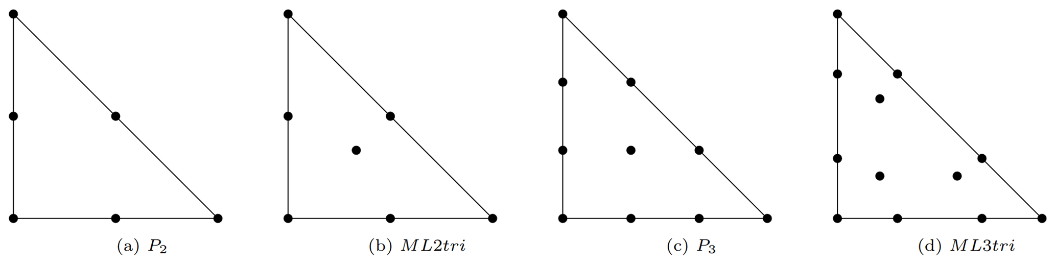
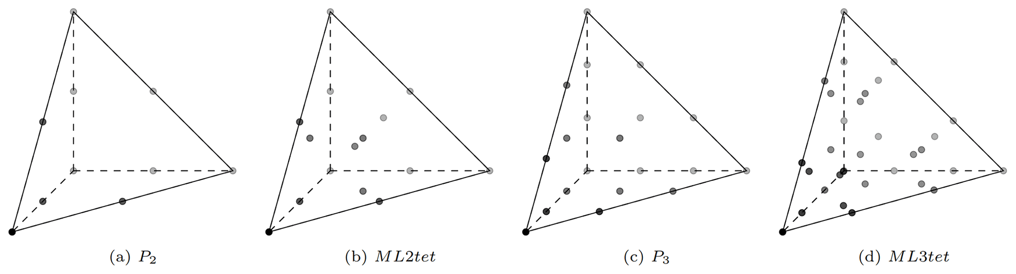
For linear triangular elements, mass lumping can be accomplished using the standard Lagrange basis functions and vertex-based Newton–Cotes integration rule. However, for higher-degree (k>1) triangular elements, a similar approach leads to unstable and/or inaccurate methods. Higher-order triangular elements and associated quadrature rules that do admit a lumping quadrature scheme are given in Geevers et al. (2018a), Chin-Joe-Kong et al. (1999), and Geevers et al. (2018b). The function spaces for these elements do not consist solely of polynomials of degree k, but also include certain higher-order bubble functions. These higher-order bubble functions increase the total number of degrees of freedom per element relative to traditional P_k elements, but in explicit time-stepping contexts, the gain of having a diagonal mass matrix more than offsets this cost (e.g., Geevers et al., 2018b; Mulder and Shamasundar, 2016).

The aforementioned concept of using higher-order bubble functions to achieve these elements is illustrated and compared with standard Lagrange elements in both 2D and 3D in Figs. 2 and 3, respectively. These elements are referred to here as mass-lumped (ML) elements. For example, ML1tri and ML1tet denotes degree-1 triangular and tetrahedral elements where the “tri” or “tet” refers to a triangular or tetrahedral element, respectively.

Figure 2 Some two-dimensional Lagrange and ML elements.

Figure 3 Some three-dimensional Lagrange and ML elements.

3.3 Waveform-adapted triangular meshes

In order to efficiently discretize the domain, a triangular mesh of conforming elements interchangeably referred to as a mesh has to be generated. The major benefit of this approach is that mesh elements range in size according to several aspects elaborated below (e.g., Fig. 4), reducing the total number of DoFs. On the contrary, for structured grids the design of the elements is fully controlled using a regular structured mesh. While a structured grid greatly simplifies applications, it imposes the additional computational cost of dramatically over resolving some areas of the domain from the standpoint of minimizing numerical error and dispersion. We note that the mesh is built by adapting elements according to the initial velocity model and is static throughout the inversion process.

The design of a so-called optimal mesh in a way that maximizes accuracy while minimizing computational cost through mesh size variation represents a challenging task. One crucial aspect is the numerical stability condition, which puts constraints on meshing because the time step is affected by the smallest cell via the Courant–Friedrichs–Lewy (CFL) condition (e.g., Mulder et al., 2013). It is crucial therefore that the mesh generation program ensures elements are as large as possible to avoid prohibitively small simulation time steps. Mesh size variation must also be gradual in order to minimize numerical error (Persson, 2006).

Figure 4 The Marmousi2 P-wave speed model (Martin et al., 2005) discretized using a graded mesh with four cells per wavelength (C=4) for a Ricker source with a peak frequency of 5 Hz. The mesh contains 3022 vertices and 5743 elements. The element size is the circumdiameter of each enclosed circle of each triangle.

In this work, variable-resolution element sizes are based on the acoustic wavelength, the CFL condition, and a mesh gradation rate. Altogether the design of resolution becomes proportional to the wavelength of the acoustic wave, hence the phrase waveform adapted. The assumption is made that all triangles will be nearly equilateral, which is necessary for accurate simulation with FEMs. The mesh can be the result of any external mesh generator; in this work we use a domain-specific mesh generator tool called SeismicMesh (Roberts et al., 2021b) that is capable of generating 2D/3D triangular meshes with the vast majority of triangles that are approximately equilateral and with elements sized according to the local seismic velocity. The desired distribution of triangular edge lengths l_e in our meshes is calculated using a ratio of the local seismic velocity (e.g., P-wave speed) and the representative frequency of a source wavelet:

$$\begin{array}{}\text{(23)}& l_{\mathrm{e}}\left(\mathit{x}\right)\propto {\displaystyle \frac{c\left(\mathit{x}\right)}{C\cdot f_{\mathrm{source}}}},\end{array}$$

where c(x) is once again the spatially variable P-wave speed, f_source is the representative frequency of a source wavelet, and C denotes the number of cells per wavelength. An example of a typical mesh size distribution for the synthetic P-wave speed model Marmousi2 (Martin et al., 2005) is shown in Fig. 4. In the case of a marine domain such as Marmousi2, the layer of water along the top of the model must contain the finest mesh resolution since the acoustic wavelength is the shortest there. It is also important to point out that mesh sizes must be smoothly varying (otherwise referred to as a graded) to avoid numerical errors when simulations are performed. In this work, we use a mesh gradation rate of 15 %, which was obtained through trial and error.

The length of the element's edges l_e can be related to the cells-per-wavelength parameter $C=\mathit{\lambda }/l_{\mathrm{e}}$, which in turn affects the number of grid points per wavelength G of a given problem. The parameters C and G are related to one another through

$$\begin{array}{}\text{(24)}& G=\mathit{\alpha }\left(P\right)\cdot C,\end{array}$$

where α(P) is a constant coefficient that is a function of the spatial polynomial degree k. ML elements have a higher number of nodes per element; therefore, they have a higher α per polynomial degree than standard Lagrange elements. Padovani et al. (1994) refer to G as the average number of grid points per space and not the maximum value of grid spacing inside the element between all possible pairwise nodal combinations. Therefore, α(P) is calculated based on the root of the number of DoFs (n_DoF) per number of elements (n_e) in the mesh, $\sqrt{n_{\mathrm{DoF}}/n_{\mathrm{e}}}$, in 2D, and $\sqrt[\mathrm{3}]{n_{\mathrm{DoF}}/n_{\mathrm{e}}}$, in 3D. When this metric is applied to SEM quadrilateral elements, it gives results that match the values reported in Lyu et al. (2020).

The selection of C, and consequently G, raises several important questions such as what is the minimal G that can minimize numerical dispersion error and how does the choice of G affect the total DoFs for a given problem? These are important aspects as they yield significant effects on both the runtime and computational requirements of FWI with FEMs and are later investigated in Sect. 5.2.

3.4 Time discretization

A second-order accurate fully explicit central finite-difference scheme was used to discretize all time derivative terms. While higher-order time-stepping schemes such as a Dablain scheme (Dablain, 1986) or a Lax–Wendroff procedure (Lax and Wendroff, 1960) can be used, these methods were not pursued in this work to better focus the paper on the aforementioned issues concerning the spatial discretization and the usage of variable-resolution triangular meshes. As a result, due to the usage of a relatively low-order time-stepping scheme, we are required to select relatively small time steps (Δt≤[1] ms) ms to ensure the error from the time discretization is sufficiently small to study the effects on the spatial discretization on the forward-state wave propagation and FWI.

For a given variable v_n=v(t_n) and for a given discrete time series t_n=nΔt, we have

$$\begin{array}{}\text{(25)}& {\displaystyle \frac{\mathrm{d}v}{\mathrm{d}t}}\left(t_n\right)\approx {\displaystyle \frac{v^{n+\mathrm{1}}-v^{n-\mathrm{1}}}{\mathrm{2}\mathrm{\Delta }t}},{\displaystyle \frac{{\mathrm{d}}^{\mathrm{2}}v}{\mathrm{d}{t}^{\mathrm{2}}}}\left(t_n\right)\approx {\displaystyle \frac{v^{n+\mathrm{1}}-\mathrm{2}{v}^n+v^{n-\mathrm{1}}}{\mathrm{\Delta }{t}^{\mathrm{2}}}}.\end{array}$$

Using this discretization and also defining a state vector as a concatenation of all the variables $Q_i^n=[U_i^n,P_i^n,Y_i^n{]}^{\mathrm{T}}$, the system of equations can be recast as

$$\begin{array}{}\text{(26)}& {\mathcal{A}}_{n+\mathrm{1}}{Q}_{n+\mathrm{1}}+{\mathcal{A}}_n{Q}_n+{\mathcal{A}}_{n-\mathrm{1}}{Q}_{n-\mathrm{1}}=\mathcal{M}{F}_n,\end{array}$$

where those new matrices are given by

$$\begin{array}{rl}& {\mathcal{A}}_{n+\mathrm{1}}=\left[\begin{array}{ccc}\mathrm{\Delta }{t}^{-\mathrm{2}}{\mathbb{M}}_u+(\mathrm{2}\mathrm{\Delta }t{)}^{-\mathrm{1}}{\mathbb{M}}_{u,\mathrm{1}}& \mathrm{0}& \mathrm{0}\\ \mathrm{0}& (\mathrm{2}\mathrm{\Delta }t{)}^{-\mathrm{1}}{\mathbb{M}}_p& \mathrm{0}\\ \mathrm{0}& \mathrm{0}& (\mathrm{2}\mathrm{\Delta }t{)}^{-\mathrm{1}}{\mathbb{M}}_{\mathit{\omega }}\end{array}\right],\\ & {\mathcal{A}}_n=\left[\begin{array}{ccc}-\mathrm{2}{\mathrm{\Delta }}^{-\mathrm{2}}{\mathbb{M}}_u+{\mathbb{M}}_{u,\mathrm{3}}+\mathbb{K}& \mathbb{D}& {\mathbb{M}}_{\mathit{\omega },\mathrm{1}}\\ {\mathbb{D}}_{u,\mathrm{2}}& {\mathbb{M}}_{p,\mathrm{1}}& -{\mathbb{D}}_{\mathit{\omega },\mathrm{3}}\\ -{\mathbb{M}}_{\mathit{\omega }}& \mathrm{0}& \mathrm{0}\end{array}\right],\\ & {\mathcal{A}}_{n-\mathrm{1}}=\left[\begin{array}{ccc}\mathrm{\Delta }{t}^{-\mathrm{2}}{\mathbb{M}}_u-\left(\mathrm{2}\mathrm{\Delta }{t}^{-\mathrm{1}}\right){\mathbb{M}}_{u,\mathrm{1}}& \mathrm{0}& \mathrm{0}\\ \mathrm{0}& -(\mathrm{2}\mathrm{\Delta }t{)}^{-\mathrm{1}}{\mathbb{M}}_p& \mathrm{0}\\ \mathrm{0}& \mathrm{0}& -(\mathrm{2}\mathrm{\Delta }t{)}^{-\mathrm{1}}{\mathbb{M}}_{\mathit{\omega }}\end{array}\right].\end{array}$$

In order to solve for the variables at time step n+1 given the previous ones, we need to invert 𝒜_n+1, which is a mass-like matrix. While this requires significant work for standard P_k elements, it is trivial for ML elements with the specialized quadrature rules discussed in Sect. 3.2.

In a practical application, it remains important to be able to determine a numerically stable time step for this discretization, and this depends on element degree k and the quality of the mesh's elements. The maximum stable time step can be estimated a priori by calculating the spectral radius of the scalar waves spatial operator while ignoring the contribution from the PML terms:

$$\begin{array}{}\text{(27)}& \mathbb{L}={\mathbb{M}}_u^{-\mathrm{1}}\mathbb{K}.\end{array}$$

A reasonable upper bound for the maximum stable time step can then be found through (e.g., Mulder et al., 2013)

$$\begin{array}{}\text{(28)}& \mathrm{\Delta }{t}_{\mathrm{CFL}}\le {\displaystyle \frac{\mathrm{2}}{\sqrt{\mathit{\rho }(\mathbb{L}})}},\end{array}$$

where ρ is the spectral radius estimated via Gershgorin's disk theorem (Geršgorin, 1931) and the subscript CFL implies an upper bound on the time step. This is possible to do explicitly for ML elements since 𝕄 is diagonal and can be inverted onto 𝕂 by just scaling rows.

In practice, a time step 10 % to 20 % lower than the estimate provided by Eq. (28) remains stable and helps ensure numerical stability can be maintained throughout the inversion process as the seismic velocity is inverted. In 3D, the spectral radius ρ(L) and consequently the maximum numerically stable time step are highly sensitive to the minimum dihedral angle in the mesh (Tournois et al., 2009). Thus, degenerate triangles termed slivers can result in exceedingly small numerically stable time steps and must be removed from the mesh. In practice, a minimum dihedral angle bound greater than 15^∘ is often desired in order to maximize the stable time step. However, this can be difficult to achieve in practice due to mesh generation challenges with variable-resolution meshes. The minimum dihedral bound can be enforced in the mesh connectivity through a sliver-removal algorithm implemented in Roberts et al. (2021b). All 3D meshes used in this work feature a minimum dihedral angle at least greater than 12^∘.

3.5 The adjoint-state and gradient problems discretized

The numerical implementation of the adjoint problem and the gradient computation are detailed in this section. From the adjoint equations presented in their strong form (Eqs. 13–15 and 16–17), we then derive the associated variational formulation through the canonical procedure:

$$\begin{array}{ll}\text{(29)}& {\displaystyle }\underset{\mathrm{\Omega }}{\int }& {\displaystyle \frac{{\partial }^{\mathrm{2}}}{\partial t^{\mathrm{2}}}}{u}^{†}v-\underset{\mathrm{\Omega }}{\int }{\displaystyle \frac{\partial }{\partial t}}\mathrm{tr}{\mathrm{\Psi }}_{\mathrm{1}}{u}^{†}v+\underset{\mathrm{\Omega }}{\int }\left(\mathrm{tr}{\mathrm{\Psi }}_{\mathrm{3}}{u}^{†}-{\mathit{\omega }}^{†}\right)v{\displaystyle }& {\displaystyle }+\underset{\mathrm{\Omega }}{\int }{c}^{\mathrm{2}}\mathrm{\nabla }{u}^{†}\cdot \mathrm{\nabla }v,\\ \text{(30)}& {\displaystyle }& {\displaystyle }+\underset{\mathrm{\Omega }}{\int }{c}^{\mathrm{2}}\left({\mathrm{\Psi }}_{\mathrm{2}}{\mathit{p}}^{†}\right)\cdot \mathrm{\nabla }v-\underset{\partial \mathrm{\Omega }}{\int }c{\partial }_t{u}^{†}v{\displaystyle }& {\displaystyle }=-\sum _{j=\mathrm{1}}^{N_{\mathrm{m}}}\left(u\right(t,{\mathit{x}}_j^{\mathrm{m}})-\stackrel{\mathrm{̃}}{u}(t,{\mathit{x}}_j^{\mathrm{m}}\left)\right)v\left({\mathit{x}}_j^{\mathrm{m}}\right),\\ \text{(31)}& {\displaystyle }& {\displaystyle }-\underset{\mathrm{\Omega }}{\int }{\displaystyle \frac{\partial }{\partial t}}{\mathit{p}}^{†}\cdot \mathit{q}+\underset{\mathrm{\Omega }}{\int }\left({\mathrm{\Psi }}_{\mathrm{1}}{\mathit{p}}^{†}\right)\cdot \mathit{q}+\underset{\mathrm{\Omega }}{\int }\mathrm{\nabla }{u}_i^{†}\cdot \mathit{q}=\mathrm{0},\text{(32)}& {\displaystyle }& {\displaystyle }-\underset{\mathrm{\Omega }}{\int }{\displaystyle \frac{\partial }{\partial t}}{\mathit{\omega }}^{†}\mathit{\gamma }+\underset{\mathrm{\Omega }}{\int }\det {\mathrm{\Psi }}_{\mathrm{1}}{u}^{†}\mathit{\gamma }-\underset{\mathrm{\Omega }}{\int }{c}^{\mathrm{2}}{\mathrm{\Psi }}_{\mathrm{3}}{\mathit{p}}^{†}\cdot \mathrm{\nabla }\mathit{\gamma }=\mathrm{0}.\end{array}$$

The discretization of this variational formulation can be cast as

$$\begin{array}{ll}\text{(33)}& {\displaystyle }{\mathbb{M}}_u{\ddot{U}}_i^{†}& {\displaystyle }-{\mathbb{M}}_{u,\mathrm{1}}{\dot{U}}_i^{†}+{\mathbb{M}}_{u,\mathrm{3}}{U}_i^{†}-{\mathbb{M}}_{\mathit{\omega }}^{\mathrm{T}}{Y}_i^{†}+\mathbb{K}{U}_i^{†}{\displaystyle }& {\displaystyle }+{\mathbb{D}}_{u,\mathrm{2}}^{\mathrm{T}}{P}_i^{†}={\mathbb{H}}^{\mathrm{T}}\mathbb{H}(U^n-{\stackrel{\mathrm{̃}}{U}}^n),\\ \text{(34)}& {\displaystyle }& {\displaystyle }-{\mathbb{M}}_p{\dot{P}}^{†}+{\mathbb{M}}_{p,\mathrm{1}}{P}^{†}+{\mathbb{D}}^{\mathrm{T}}{U}_i^{†}=\mathrm{0},\text{(35)}& {\displaystyle }& {\displaystyle }-{\mathbb{M}}_{\mathit{\omega }}{\dot{Y}}_i^{†}+{\mathbb{M}}_{\mathit{\omega },\mathrm{1}}^{\mathrm{T}}{U}_i^{†}-{\mathbb{D}}_{\mathit{\omega },\mathrm{3}}^{\mathrm{T}}{Y}_i^{†}=\mathrm{0},\end{array}$$

where ℍ is the discrete version of the Dirac operator applied on all the measurement points in the domain. We remark that all the matrices used before (see Appendix B) are reused but transposed (if not symmetric) both at the level of their entries and at the level of the equations. By discretizing the continuous equations with the FEM, we obtain the discrete adjoint. This is further clarified when discretizing Eq. (33) in time using the same procedure as before with central differences (e.g., Eq. 25), which leads to the system for the variables in compact notation $Q^{†}=(U^{†},P^{†},Y^{†}{)}^{\mathrm{T}}$:

$${\mathcal{A}}_{n+\mathrm{1}}^{\mathrm{T}}{Q}_{n-\mathrm{1}}^{†}+{\mathcal{A}}_n^{\mathrm{T}}{Q}_n^{†}+{\mathcal{A}}_{n-\mathrm{1}}^{\mathrm{T}}{Q}_{n+\mathrm{1}}^{†}={\mathcal{H}}^{\mathrm{T}}\mathcal{H}(Q^n-{\stackrel{\mathrm{̃}}{Q}}^n).$$

In addition to the adjoint, the gradient is computed by discretizing Eq. (19) by letting the function δc to be the trial function. The resulting linear system for the gradient, denoted 𝒢 in its discrete form, is written as

$$\begin{array}{ll}\text{(36)}& {\displaystyle }\mathbb{M}\mathcal{G}& {\displaystyle }=\mathcal{R},\text{where}{\mathcal{R}}_l=\sum _{i=\mathrm{1}}^{N_{\mathrm{s}}}\sum _{n=\mathrm{1}}^{N_t}\underset{\mathrm{\Omega }}{\int }\mathrm{2}c\mathrm{\nabla }{u}_i^{†}\left(t_n\right){\displaystyle }& {\displaystyle }\cdot \mathrm{\nabla }{u}_i\left(t_n\right)\mathit{\delta }{c}_l\mathrm{d}\mathit{x}.\end{array}$$

In order to derive the discrete adjoint and gradient, the time integrals appearing in the continuous formulation (i.e., in the cost functional J, and in the definition of the inner product, in the Lagrangian functional ℒ) were all replaced with discrete sums that did not consider a time integration. This is a similar approach to what was performed in Bunks et al. (1995). For this reason, no Δt factor (or other time integration methods such as trapezoidal or Simpson's rule) is present.

Also, we stress here that, in order to obtain the gradient 𝒢, we need to solve Eq. (36) by inverting a mass matrix. This matrix comes from the fact that, in the continuous gradient derivation, Eq. (19), the inner product is chosen to be the classical L² inner product, which is represented by the mass matrix in the discrete framework. This choice of inner product ensures that the gradient will be mesh-independent (e.g., Schwedes et al., 2017) in the sense that local mesh refinements will not produce differences in the gradient (if the problem is sufficiently mesh-converged). For example, if the right-hand-side expression in Eq. (36) is readily used as the gradient, the mesh dependency would be present as the space integration would only be present on the right-hand side.

3.6 Gradient subsampling

Numerical simulations often require several thousand time steps integrating over several seconds with the aforementioned numerical approaches to compute the discrete gradient. As a result, there are significant memory requirements for storing the forward-state solution that is necessary to calculate $\stackrel{\mathrm{̃}}{Q}$ and subsequently 𝒢. By considering that the numerically stable time step given by the CFL condition is generally much shorter than the Nyquist sampling frequency dictated by the maximum source frequency, our implementation allows for a subsampling approach to calculate 𝒢 to reduce memory overhead. In other words, the forward state can optionally be saved at every r time steps (r≫1), where r is the subsampling ratio, and subsequently the gradient is calculated every r time steps. It is noted that this is known to lead to artifacts and inexact gradients and requires careful tuning to ensure feasible memory runtime requirements while balancing the accuracy of the gradient. The r subsampling factor is noted in the results. These aspects were extensively studied in Louboutin et al. (2019).

4 Computer implementation

In this section, important components of our implementation are explained. The Firedrake package is used to implement the numerical developments. The code (Roberts et al., 2021a) and data sets (Roberts, 2021) together with Firedrake (firedrake-zenodo, 2021) were used for all experiments.

An additional layer of implementation is necessary for applications in seismic problems as there are operations to execute FWI that fall outside of the capabilities within the Firedrake package. It is important to mention that Firedrake has components that allow us to compute the gradient with automatic differentiation (AD) (e.g., dolfin-adjoint, Mitusch et al., 2019), and we have made the necessary additions to spyro that enable the use of this functionality to perform FWI. However, at the time the results for this paper were generated, that was not ready yet, and we have performed all calculations solving the adjoint equations inserted directly in the algorithm.

The Rapid Optimization Library (ROL; Cyr et al., 2017) is used to solve the inverse problem given a gradient, a cost functional, and a method to update the velocity model. The ROL library provides interfaces to and implementations of various algorithms for gradient-based, unconstrained and constrained optimization coupled with line-search conditions that satisfy the strong Wolfe conditions (Wolfe, 1969). This improves the robustness of our FWI code by using well-developed and tested algorithms. The C++ library ROL is called in our Firedrake Python codes via a Python wrapper code called pyROL (Wechsung and Richardson, 2019). ROL was preferred over SciPy’s optimization library because the Firedrake development team is actively involved with the developers of the ROL interface. Further, the usage of ROL allowed for more advanced optimization methods than SciPy offered.

As mentioned earlier in this work, we exclusively rely on the second-order optimization method L-BFGS (Byrd et al., 1995), which includes information about the curvature of the misfit function in the optimization process (Eq. 10). The benefit of using second-order optimization methods in FWI has been studied previously and shown to benefit the computational efficiency of FWI (e.g., Castellanos et al., 2014). Using pyROL and Firedrake, a conventional FWI approach can be written in several dozen lines of Python.

Given the gradient subsampling (see Sect. 3.6), the precision of the gradient was not severely damaged by subsampling. This aspect was verified to ensure that the shape of the gradient remained essentially the same as without the subsampling. It is true, however, that if the frequency of the subsampling is not high enough, the gradient can be damaged, typically when the wave traveling one mesh element of size h and experiencing a wave speed c is sampled with fewer than, say, five points, leading to a condition of the form $\mathrm{d}t<\mathrm{5}h/c$.

4.1 Implementation of higher-order mass-lumped elements

Five triangular elements for spatial polynomial degrees k≤5 from Chin-Joe-Kong et al. (1999) and three tetrahedral elements for spatial polynomial orders up to k=3 (Geevers et al., 2018b) were implemented inside the Finite element Automator Tabulator package (FIAT, Kirby, 2004). In particular, we use the latest documented k=3 3D tetrahedral element ML3tet from Geevers et al. (2018b) with 32 nodes. This program FIAT is used by the Firedrake package to tabulate a wide variety of finite-element bases.

The quadrature rules are key to defining the finite-element basis, so we began by implementing these within FIAT. Then, to define the finite elements themselves, we must first construct the function space. This is done using two particular FIAT features described in Kirby et al. (2012). First, we use the RestrictedElement operation on a Lagrange element to remove bubbles from facets where enrichment occurs, and then we use a NodalEnrichedElement operation to introduce higher-order bubbles into those facets. Second, we must provide the dual basis, which is just a list of pointwise evaluation functionals associated with the ML quadrature points. In addition to these, like all other FIAT elements, we also provide a topological association of the degrees of freedom to facets, and this information is used at a higher abstraction level by Firedrake to build local-to-global mappings.

Certain standard boilerplate is required to expose a new FIAT element to the rest of Firedrake. First, the element, along with certain metadata, must be announced within the Unified Form Language. Then, it must also be wrapped into FInAT (Homolya et al., 2017), which is a layer that provides abstract syntax for basis evaluation and supports higher-order operations, such as tensor products of elements or making vector-valued spaces such as used for our p variable. It is this layer, rather than FIAT itself, that interacts with Firedrake's form compiler, tsfc (Homolya et al., 2018). Within tsfc, we must also provide a binding between UFL names and FInAT classes. Hence, although we make changes to several packages, they are rather superficial beyond the FIAT implementation.

4.2 Receivers and sources

To probe the computational domain, functionality is required to both record the solution at a set of points (i.e., receivers) and to inject the domain with a time-varying wavelet (i.e., sources; Fig. 1). Since the location of receivers does not necessarily match vertices exactly inside the mesh connectivity, the wave solution must be interpolated to the receiver locations. Interpolation of the wave solution to the receivers is carried out in the same space of the finite elements used to discretize the domain.

Source injection is the adjoint operator of interpolating the solution to the receivers. To execute both, a Dirac mass is integrated against the finite-element basis functions in the form of weights equal to the basis functions evaluated at the source (receiver) position inside the element that contains the source (receiver). This point force source is of the form f=w(t)δ_x(x), where w(t) denotes the wavelet and x_s the source or receiver position. For the 2D case, the contribution to $f_{g(j_{\mathrm{s}},k),l}$ is ${\int }_{{\mathcal{T}}_{j_{\mathrm{s}}}}f{\mathit{\varphi }}_{j_{\mathrm{s}},k}\mathrm{d}x=w\left(t\right){\mathit{\varphi }}_{j_{\mathrm{s}},k}\left(x_{\mathrm{s}}\right)$. Here g(j_s,k) defines the local-to-global map from node k in element j containing the s source/receiver to the global set of DoFs. For the adjoint calculation, the source is forced at the receiver locations that recorded the solution in the forward-state problem.

4.3 The inversion process

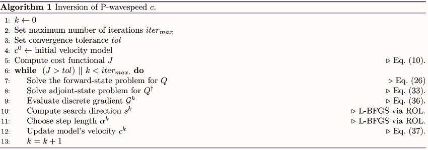
We start with an initial distribution of P-wave speed c and solve the forward-state problem to obtain Q. With the misfit known, we then solve the adjoint-state problem and obtain Q^†. With both Q and Q^† known the discrete gradient 𝒢 can be computed. Thus, the updated velocity model c can be computed by

$$\begin{array}{}\text{(37)}& c^{k+\mathrm{1}}=c^k+{\mathit{\alpha }}^k{s}^k,\end{array}$$

where α^k is the step length, s^k is the search direction, and the superscript k denotes the iteration. In the L-BFGS algorithm, the computation of the descent direction s^k is done using an approximation of the Hessian matrix, computed by finite difference of previous gradient evaluations. Also, the step length is computed satisfying the Wolfe conditions (see Byrd et al., 1995). Both are automatically taken care of by the implementation in ROL.

The discussed inversion process is shown in Algorithm 1. In order to ensure a sufficient decrease of the objective functional at each inversion iteration k, line-search conditions are employed that satisfy the strong Wolfe conditions (Wolfe, 1969). This line search is implemented inside the ROL library.

4.4 Wave propagators

The spatial and temporal discretizations detailed in Sect. 2.1 are programmed with Firedrake. Figure 5 illustrates the main functions – forward.py and gradient.py – and how they work together. The forward wave propagator called forward.py returns two quantities for a given source configuration: the Q at the time steps determined by the subsampling ratio r (see Sect. 3.5) and the forward-state solution ℋQ at the receivers for all time steps. The adjoint-state propagator takes as input the difference between measured and modeled data at the receiver locations (otherwise referred to as the misfit) and the forward-state solution Q. To conserve virtual memory, while the adjoint-state propagator executes, the function called gradient.py discards Q as the adjoint Q^† and subsequently 𝒢 (Eq. 36) is calculated backward in time. Note that the adjoint wave propagator returns the gradient summed over the time steps dictated by the subsampling ratio r (see Sect. 3.5).

Figure 5 The functionality of the forward-state, adjoint-state, and gradient Python codes.

We point out that all spatial discretizations are performed using matrix-free approaches, which are available in the Firedrake computing environment, and this reduces runtime memory requirements (e.g., Homolya et al., 2017; Kirby and Mitchell, 2018).

4.5 Two-level parallelism strategy

A two-level parallelism strategy is implemented over both the sources and spatial domain decomposition. In space, domain decomposition parallelism is handled by the Firedrake library, which automatically handles setting up halo/ghost zones around each subdomain and performing the necessary communication at each time step via the Message Passing Interface (MPI). In addition, Firedrake also provides options to configure the depth of the ghost layer for performance as needed. In this work, no ghost layers are added to the subdomains, and instead the solution is shared only at the boundary nodes of each subdomain. At the source level, parallelism is trivial and handled by splitting the MPI communicator into groups of processes at initialization and assigning each group to simulate one source. Due to the usage of Firedrake, no additional code is required for parallelism as compared to the sequential version of the code.

We do note a significant benefit from using both shot-level and domain decomposition parallelism simultaneously, especially in 3D, which is later detailed in Sect. 5.3.

4.6 Meshes and file I/O

Mesh files are read in from disk sequentially and then distributed in parallel if necessary; this functionality is handled latently by Firedrake. External seismic velocity models are read in from disk from an H5 file format at execution time. Gridded velocity data are bi-linearly interpolated onto the nodal DoFs of the elements of the mesh at runtime. In this way, seismic velocities can vary inside the element in the event higher-order elements are used. Gridded seismic velocity files can be prepared using SeismicMesh (Roberts et al., 2021b)

5 Computational results

5.1 Numerical verification of discrete gradient

The accurate computation of the discrete gradient is crucial for the robustness of Algorithm 1. Through a numerical experiment, we demonstrate that the gradients computed through the optimize-then-discretize approach (see Sect. 3.5) are approximately equal to the discrete gradients computed by the discrete gradients of the discrete objective functional. In this way, we compare the directional finite difference of the discrete objective functional. The finite-difference directional derivative is given as a forward finite difference:

$$\begin{array}{}\text{(38)}& d_h^{\mathrm{fd}}\left(c\right)\left(\stackrel{\mathrm{̃}}{c}\right):={\displaystyle \frac{J(c+h\stackrel{\mathrm{̃}}{c})-J\left(c\right)}{h}},\end{array}$$

where $\stackrel{\mathrm{̃}}{c}$ is the discrete direction for c and h is an arbitrarily small step size. The directional derivative obtained via the control problem is

$$\begin{array}{}\text{(39)}& d^{\mathrm{co}}\left(c\right)\left(\stackrel{\mathrm{̃}}{c}\right)={\stackrel{\mathrm{̃}}{c}}^T\mathbb{M}\mathcal{G}.\end{array}$$

Next, we verify that Eqs. (38) and (39) produce accurate values for an arbitrary choice of $\stackrel{\mathrm{̃}}{c}$ considering the test problems displayed in Fig. 6. For this test, the direction $\stackrel{\mathrm{̃}}{c}$ to test is that of the gradient G.

The considered 2D test problem to verify the numerical gradients was a physical domain Ω₀=1.0 × 1.0 km that features half the domain with a P-wave speed of 4.0 km s⁻¹ and the other half with a P-wave speed of 1.0 km s⁻¹ (Fig. 6a). The physical domain was truncated with a 200 m PML on the sides while a non-reflective Neumann boundary condition was applied at the top. A 5 Hz source is injected at $(-\mathrm{0.1},\mathrm{0.50})$ km, and the solution is recorded at 100 receivers equispaced along a horizontal line at the bottom of the domain between $(-\mathrm{0.90},\mathrm{0.1})$ and $(-\mathrm{0.90},\mathrm{0.90})$ km. In this configuration, the problem models a transmission of an acoustic wave. The domain was discretized with uniform-sized ML2tri elements with l_e=20 m in length yielding G>10 given the 5 Hz peak source frequency, which we found is sufficient for this experiment. The total duration of the simulation is 1.0 s, which is long enough for the wave to be absorbed in the PML and transmitted to the receivers. A computational time step Δt=0.50 ms was used, and the gradient was computed with all time steps (r=1). Note that the directional derivative (Eq. 39) was integrated only in Ω_physical and masked in Ω_PML.

In 3D a similar problem to the 2D case was considered within a physical domain Ω₀=1.0 × 1.0 × 1.0 km. Note the orientation of the axes is z, x, and then y. A 5 Hz source located was injected at $(\mathrm{0.1},\mathrm{0.50},\mathrm{0.50})$ km, and the solution was recorded at a 2D grid of 100 receivers equispaced apart in both x and y directions at the bottom end of the domain between $(\mathrm{0.90},\mathrm{0.1},\mathrm{0.1})$ km and $(\mathrm{0.90},\mathrm{0.90},\mathrm{0.90})$ km (Fig. 6(b)). The domain was discretized with uniform ML2tet with l_e=20 m in length yielding G>10. A computational time step Δt=0.50 ms is used, and the gradient was computed with all time steps (r=1). Similar to the 2D case, the gradient was masked in Ω_PML.

For both 2D and 3D cases, an initial velocity model with a uniform velocity of 4.0 km s⁻¹ was used; however, we simulated both the exact and initial models with the same mesh.

Table 1 Comparison of directional derivatives for 2D and 3D cases between the finite-difference approximation (fd) and our discrete gradient (co).

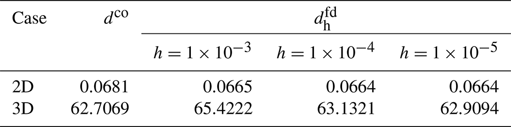
We point out that relatively good agreement was found between the two derivatives in which the wave field was resolved with at least G=10 (Table 1), especially in the 2D case where the maximum relative difference between the gradients was less than 0.03 %. In the 3D case, the discretization error becomes somewhat larger and results in maximum relative differences of approximately 4.0 %, decreasing with smaller h.

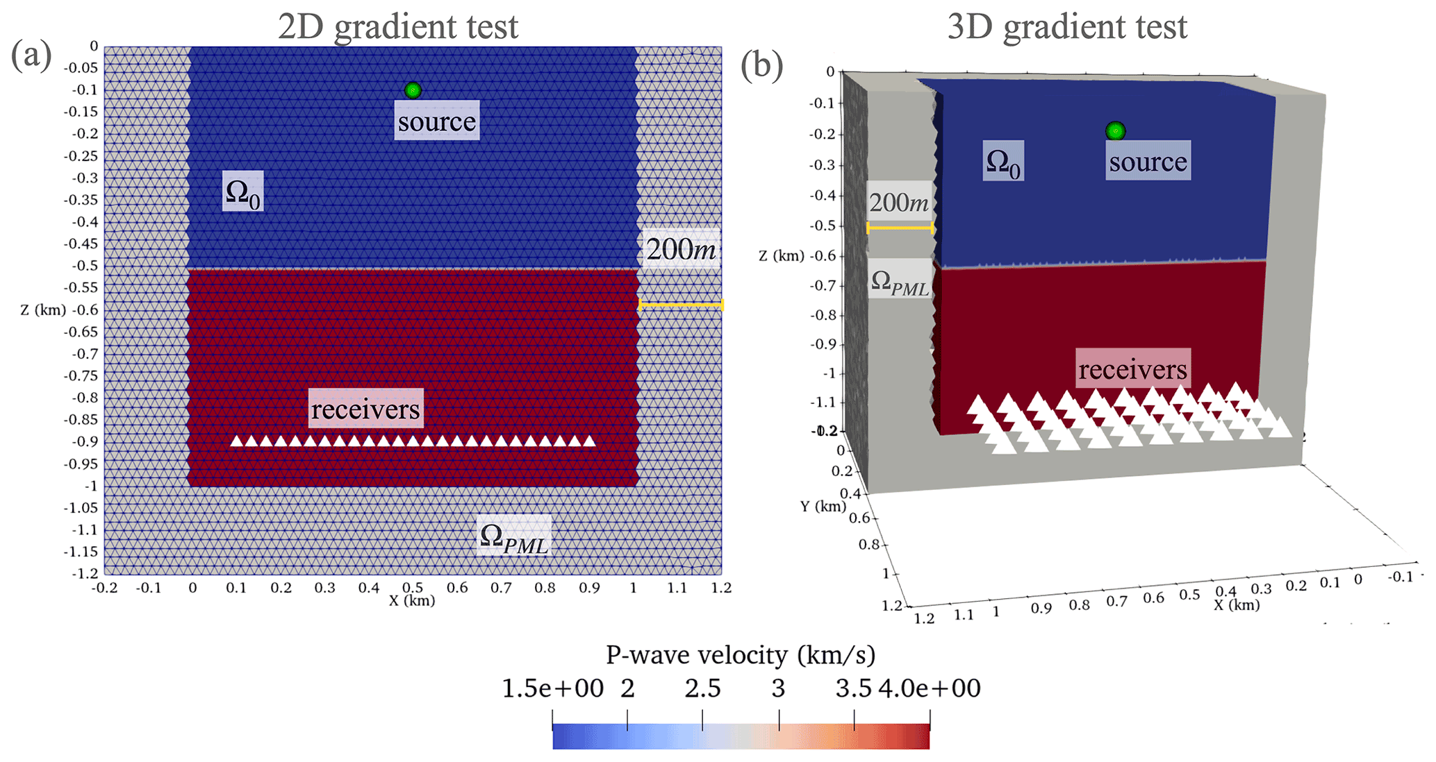
Figure 6 Problem configuration for verification of the discrete gradient in (a) 2D and (b) 3D. Note not all receiver positions are shown for visualization purposes.

5.2 On the design of waveform-adapted meshes

To effectively apply higher-order mass-lumped methods with unstructured meshes, it is important to understand the required mesh resolution for a given desired accuracy (Lyu et al., 2020; Geevers et al., 2018c). As mentioned in Sect. 4.1, ML elements contain a greater number of DoFs per element than standard CG Lagrange or spectral/hp collapsed triangular elements. This does not imply, however, that a given problem would contain a greater number of DoFs when discretized with ML elements since mesh resolution requirements for each method and element type vary widely (Lyu et al., 2020). Similar to the works of Geevers et al. (2018c) and Lyu et al. (2020), we investigate the accuracy of ML elements for forward-state wave propagation to guide their application in FWI.

5.2.1 Reference wave field solution

The implementation of the forward-state wave propagator in 2D and 3D was first verified in order to reliably intercompare solutions between elements. An equivalence was demonstrated between a converged numerical result computed on a highly refined mesh in 2D and 3D and compared with their analytical solutions, respectively. Following that, the assumption was made that equivalence holds for all our subsequent tests, implying that all the reference waveforms are converged numerical solutions, given sufficiently fine mesh resolution and sufficiently small numerical time steps.

The method of manufactured solutions (MMS) was used to verify the implementation in accordance with a manufactured analytical solution. The manufactured 2D analytical solution was chosen as t²sin (x)sin (y). In 3D the analytical solution was t²sin (x)sin (y)sin (z). Both analytical solutions are defined on a unit square and unit cube with a 250 m wide PML layer. Numerical solutions were calculated on highly refined reference meshes built with G=14.07 using ML5tri in 2D and G=9.30 using ML3tet in 3D. The velocity model was homogeneous with [1.43] km s⁻¹. The simulations used a time step of Δt=1 ms and were integrated for 0.10 s. The MMS error was represented as the L2 norm between the analytical and numerical solution normalized by the analytical solution and only measured in the physical domain.

Our experiments demonstrated good agreement between the analytical and modeled solutions with a relative error for the 2D reference homogeneous case of 0.34 %, and for the 3D homogeneous case the relative error was 0.90 %. These error values indicate the reference solutions represent numerically converged results given the spatial discretization, and the forward-state code implementation is producing correct solutions.

5.2.2 Homogeneous 2D P-wave speed model

A 2D wave propagation experiment in a domain with a homogeneous velocity field was configured to quantify the accuracy of the forward-state solution with ML elements (Fig. 7). The experiment is similar in design to that analyzed in Lyu et al. (2020), which an SEM of variable space order. A domain of 40.0λ by 30.0λ (i.e., 11.4 km by 8.57 km) was generated, where λ is the wavelength of the acoustic wave given the model's wave speed. The model had a uniform wave P-wave speed of 1.43 km s⁻¹, which is approximately the speed of sound in water. A Ricker wavelet with a peak source frequency of 5.0 Hz was injected at the center of the domain, and a grid of 36 receivers was placed at a 10.0λ (i.e., 2.86 km) offset to the right of the source location in order to record and intercompare solutions (Fig. 7). A 0.28 km PML layer was added to absorb outgoing waves. The time step used for each simulation was 20.0 % less than the Δt_CFL estimated maximum stable time step (see Sect. 3.4). Meshes were generated for each element type by varying the C, which resulted in G that ranged from G=2 to G=10.5. Results were compared against the solutions computed on the so-called reference meshes.

Error was calculated based on the simulated pressure recorded at the receiver locations with

$$\begin{array}{}\text{(40)}& E=\sqrt{{\displaystyle \frac{{\sum }_{r=\mathrm{1}}^{N_{\mathrm{r}}}{\int }_{\mathrm{0}}^{t_{\mathrm{f}}}(p_{\mathrm{r}}-p_{r_{\mathrm{ref}}}{)}^{\mathrm{2}}\mathrm{d}t}{{\sum }_{r=\mathrm{1}}^{N_{\mathrm{r}}}{\int }_{\mathrm{0}}^{t_{\mathrm{f}}}{p}_{r_{\mathrm{ref}}}^{\mathrm{2}}\mathrm{d}t}}}\times \mathrm{100}\mathit{\%},\end{array}$$

where N_r denotes the number of receivers, t_f is the final simulation time in seconds, p_r is the pressure at the receivers for a given mesh, and p_ref denotes the pressure at the receivers computed with a reference mesh. The time integration in Eq. (40) was computed using the trapezoidal rule. Eq. (40) is a measure in percent difference between two solutions at the same set of receivers. It is important to point out that measuring E in this way combines the error associated with receiver and source interpolation as well as from the wave propagation. When E is measured at one receiver at a particular offset coordinate x, this is referenced by a subscript (e.g., $E_{\mathit{x}=(\mathrm{0.5},\mathrm{0.5})}$); otherwise, the quantity E considers all receivers.

The space of E for several values of C and subsequently G was explored for different ML elements in a process referred to as a grid sweep (Table 2). The objective of the grid sweep is to find the smallest G (i.e., lowest grid point density) that can produce E at or below a specified threshold. An allowable tolerance of E=5.0 % for each ML element was selected. While the E=5.0 % threshold chosen is arbitrary, it represents a measurement that can be used to intercompare solutions and, as we later show through application, to be sufficiently accurate for robust FWI. Further, smaller target thresholds for E led to non-convergence for some elements. To execute the grid sweep, the value of G was varied within a range of values depending on the change in E in a similar manner to a back-tracking line search.

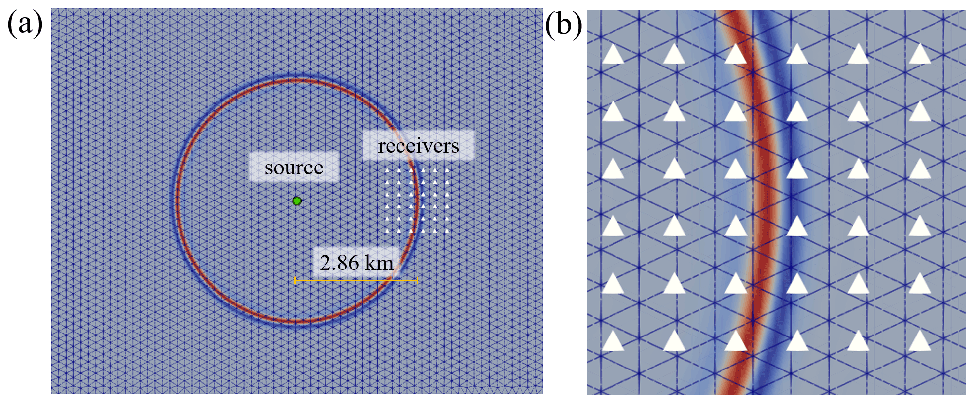
Figure 7 The experimental configuration to calculate the grid-point-per-wavelength G values. In panel (a) the source is shown as a green circle and the receivers are denoted as white triangles with a close-up of the bin of receivers shown in panel (b). In both panels, the normalized wave field is colored at t=2.25 s.

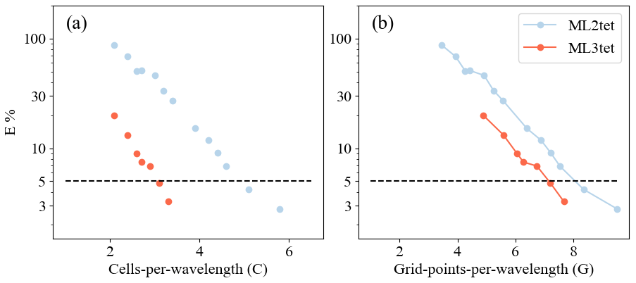
Figure 8 Panels (a) and (b) depict results for the homogeneous velocity model experiment to find the minimum G (Sects. 5.2.2 and 5.2.3). Panel (a) shows C as a function of E (Eq. 40). Panel (b) illustrates the E as a function of G. Panels (c) and (d) show the same thing as panels (a) and (b) but for the heterogeneous velocity model experiment. Colored lines represent the spatial polynomial order of the element. The E=5 % threshold is drawn as a horizontal dashed black line on all panels.

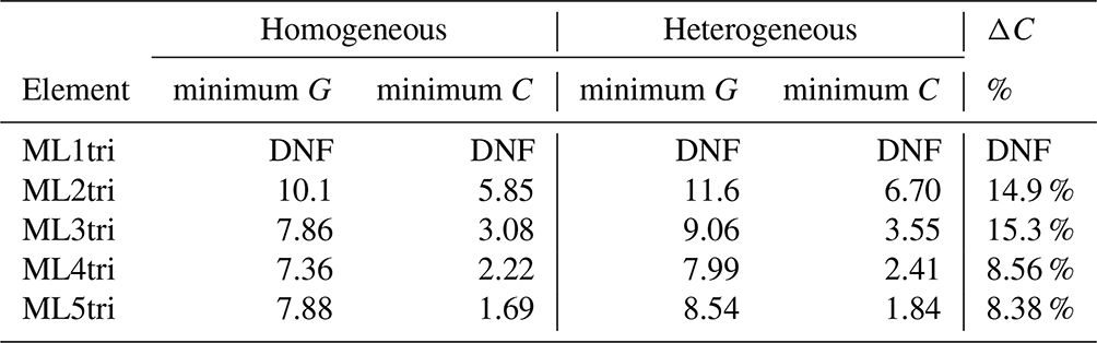
Table 2 Results from the grid sweep for both the homogeneous and heterogeneous experiment to identify efficient values for G using ML elements of varying spatial degree k that maintain an error threshold of E=5 %, as compared to a highly refined reference solution (see Sect. 5.2). Note that DNF stands for did not finish.

Overall, the homogeneous grid sweep results demonstrate that elements with spatial order k>2 required fewer G to achieve the same E than ML2tri. As expected, the necessary C in order to maintain the target E decreases as spatial polynomial order is increased (Fig. 8b). The relationship between C and G is not linear due to the higher-order bubble functions inside the ML elements (see Sect. 3.2). Thus, the convergence rate of E with respect to G is not as consistent as it is for C (Fig. 8a).

Applying the results from the homogeneous grid sweep, the values for G and C that achieved E=5.0 % are shown in Table 2. The variation in C that could achieve the E threshold was C=1.69 to C=5.85 for ML5tri to ML2tri, respectively, while for G it varied between G=7.36 and G=10.1. The ML element that led to the smallest problem (e.g., minimum G) while satisfying the target E was ML4tri with G=7.36, whereas ML2tri required G=10.01. It is important to note that the lowest-order ML1tri element performed poorly and did not achieve the target for E with any configuration of C tested.

5.2.3 Heterogeneous 2D P-wave speed model

In addition to generating a mesh that meets the requirements of the technique used to numerically discretize the PDE, the mesh must also account for local variations in the seismic velocity, which can have significant effects on the simulation of acoustic waves. In the case of simulation with a heterogeneous velocity model, E combines errors associated with how the mesh discretely represents the local variations in velocity and errors associated with numerical discretization techniques. Thus, it is often necessary to add additional DoFs into the design of the unstructured mesh above what would be required for a homogeneous seismic velocity model to accurately represent local seismic features (e.g., Anquez et al., 2019; Seriani and Priolo, 1994; Lyu et al., 2020). However, it is important to point out that in FWI applications, the inversion commences from a smooth, initial velocity model (e.g., Fathi et al., 2015; Thrastarson et al., 2020; Trinh et al., 2019), with locations of velocity interfaces that are not generally not known prior.

As a result, in this experiment we added an additional percent to the parameter values of C obtained from the homogeneous test case (Sect. 5.2.2). The percent difference in C between homogeneous and heterogeneous results is defined as ΔC:

$$\begin{array}{}\text{(41)}& \mathrm{\Delta }C={\displaystyle \frac{(C_{\mathrm{het}}-C_{\mathrm{hom}})}{C_{\mathrm{hom}}}},\end{array}$$

where the subscripts “het” and “hom” denote the heterogeneous and homogeneous grid sweep results, respectively.

For triangular meshes, the ΔC that is necessary to minimize E when simulating with heterogeneous velocity models has not been investigated in prior scientific literature to the authors' knowledge. It is also important to determine how the previously described homogeneous results can be applied to a heterogeneous seismic velocity model.

In a similar manner to the experiment with the homogeneous velocity model, a 2D experiment with a heterogeneous velocity model was performed for the BP2004 P-wave speed model (Billette and Brandsberg-Dahl, 2005) (Fig. 9). The BP2004 model represents geologic features in the eastern/central Gulf of Mexico and offshore Angola and is characterized by several salt bodies with P-wave speeds >4 km s⁻¹. The domain is 12.0 km by 67.0 km with an additional 1.00 km PML. A Ricker source was injected at (−1.0, 34.5) km, and a horizontal line of 500 receivers from (−1.0, 36.5) to (−1.0, 44.5) km was used to record the wave field solution. The acquisition geometry led to a near offset of 2.00 km and a far offset of 10.0 km from the source location, which are common dimensions in marine FWI applications for seismic velocity building (e.g., Virieux and Operto, 2009). Each simulation lasted 9.0 simulation seconds, which was sufficient time for reflected waves to reach the receivers with the largest offsets.

In the mesh generation process, a mesh gradation rate of 15.0 % was enforced to bound the element size transitions (Fig. 9). As with the homogeneous experiment, G=6 to G=12 were evaluated by comparing to the reference case. The reference case used a highly refined mesh constructed with G=15.0 and simulated with ML5tri elements, which could correctly resolve all interfaces (Fig. 9).

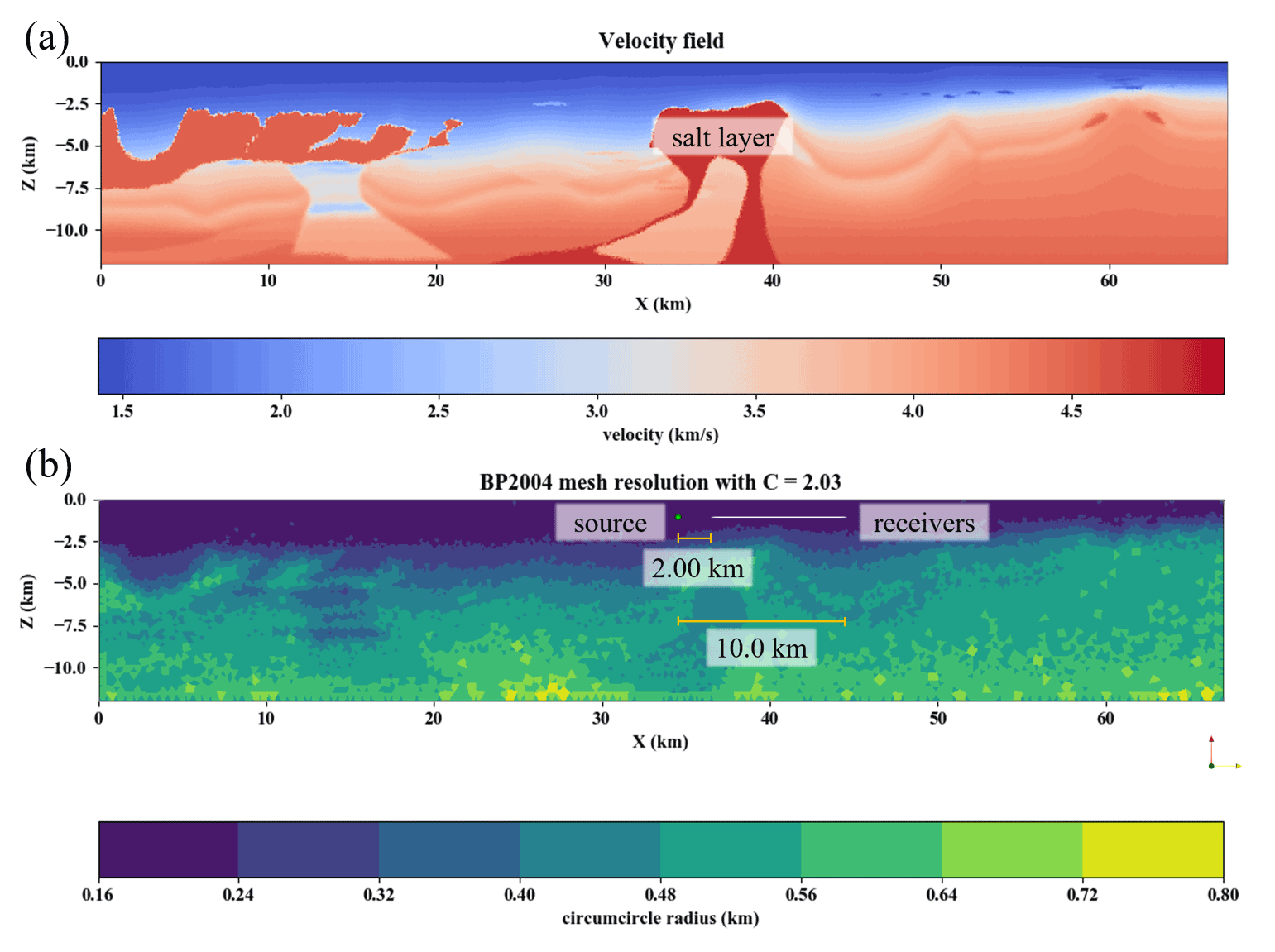
Figure 9 The reference problem configuration for the BP2004 seismic velocity model. Panel (a) shows the P-wave speed data. Panel (b) shows the mesh resolution (circumcircle diameter) based on local adaptation of the mesh resolution to the P-wave data from the BP2004 velocity model shown in panel (a). The parameters used for mesh generation were C=2.03, ML5tri, a velocity gradation rate of 15.0 %, and an anticipated time step of Δt=0.001 ms.

As shown by Fig. 8c–d, the experiments with the BP2004 model consistently exhibited greater E and slower convergence rates as compared to the values from the homogeneous experiment given the same G (see Fig. 8a). As a result, the values for C used to generate the meshes were increased from what was found in the homogeneous experiment by ΔC=20.0 % and resulted in acceptable errors of E=3.45 %, E=3.82 %, E=3.44 %, and E=3.38 %, for ML2tri, ML3tri, ML4tri, and ML5tri elements, respectively. ΔC less than 20.0 % did not sufficiently reduce the error to under the E=5.0 % threshold.

Wave propagation errors can be the result of dispersion and also show how well the mesh represents the local seismic wave speed variations. In our mesh design, exact fault locations were not resolved with edge-orientated elements (e.g., Anquez et al., 2019), and our numerical discretization used elements from a continuous function space; thus, error associated with the propagation of the reflected wavelet in the sharp contrast of the salt layer is expected. This error becomes more pronounced when using larger element sizes associated with the higher-order (k>2) ML elements. As an example of this, in Fig. 10 E is calculated individually for each receiver as a function of offset for ML5tri. A peak of E=7.71 % occurred at the offset of 2.21 km that is associated with the reflection brought on by the salt layer Fig. 11 and results in the peak E not only in ML5tri but also in ML3tri and ML4tri. Neglecting the E associated with the salt body reflection in this receiver location would reduce the error from E=7.71 % to E=2.02 %. Furthermore, even though E was kept below the previously defined threshold, a small dispersion error still exists and can be noted in receivers at the far offset in all cases. Dispersion error was the most prevalent error only in the lower-order ML2tri element, whereas in ML3tri, ML4tri, and ML5tri the greatest error came from the wavelet reflected by the salt layer.

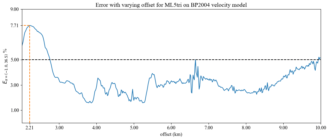
Figure 10 E (Eq. 40) as a function of the offset distance for ML5tri in the heterogeneous model setup. Peak E is annotated with dashed orange lines.

For ML3tri, ML4tri, and ML5tri elements, peak E stemmed from the reflected wave associated with the salt body due to the enlargement of element sizes near the salt body (Fig. 11). Figure 11b illustrates the moment when the wave reflects off of the salt body and this reflected wave accounted for 73.8 % of the total error at this receiver.

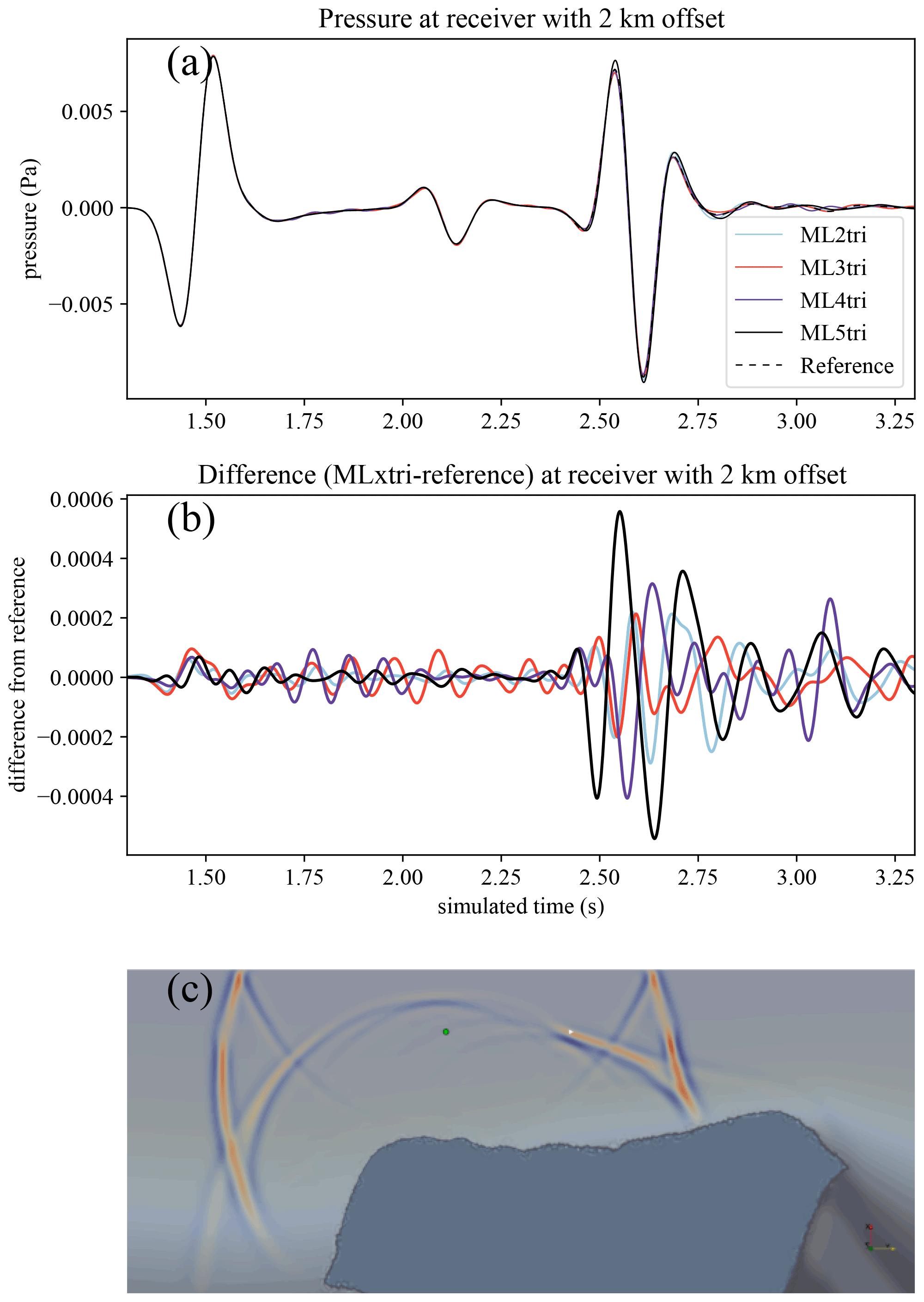
Figure 11 Panel (a) shows time series of pressure for several elements measured at a receiver with an offset of 2.00 km. The difference (MLxtri − reference) in signals from the reference case is shown in panel (b), where x varies from 2 to 5. Panel (c) is the wave field at t=2.53 s with the receiver at 2.00 km emphasized with a triangular glyph. The difference in the signals is greatest when the wave reflected by the salt body (indicated by darker blue in panel c) passes through the receiver also illustrated in panel (c).

5.2.4 Homogeneous 3D P-wave speed

A similar experiment to that described Sect. 5.2.2 was used to assess 3D ML elements. The focus was placed on finding suitable values for C and G that minimize error for the ML2Tet and the ML3Tet elements that were discovered in Geevers et al. (2018c). Therefore, a homogeneous 3D model was created with a uniform P-wave speed of 1.43 km s⁻¹ in a $\mathrm{15.0}\mathit{\lambda }\times \mathrm{30.0}\mathit{\lambda }\times \mathrm{15.0}\mathit{\lambda }$ (i.e., 4.29 km by 8.57 km by 4.29 km) domain with an added 0.28 km PML layer to absorb outgoing waves on the sides and bottom. A Ricker wavelet source was added at the coordinate (2.14, 0.43, 2.14 km), and 216 point receivers were arranged in a cubic grid with a width of 5λ (i.e., 1.43 km) that was placed at a center offset of 10λ (i.e., 2.86 km) to the right of the source coordinate, as illustrated in Fig. 12. The time step used for each simulation was 20.0 % less than the Δt_CFL (maximum stable time step based on an estimate) (see Sect. 3.4). As with Sect. 5.2.2, meshes were generated by varying C, and a back-tracking line search was executed to reach an error threshold of 5.0 % calculated using Eq. (40).

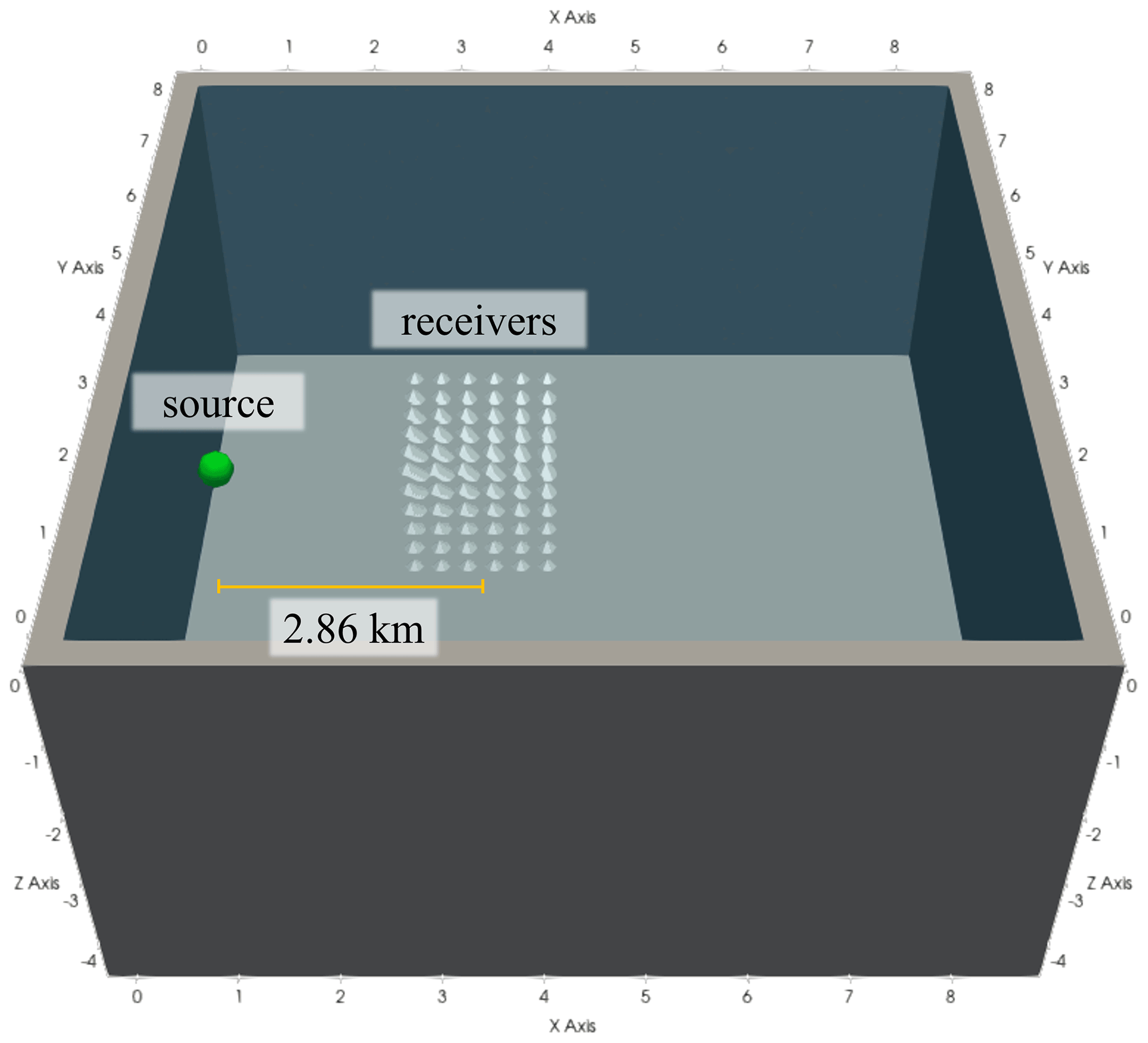
Figure 12 The 3D experimental configuration to calculate the grid-point-per-wavelength G values. The Ricker source is represented as a green sphere, and the receivers are denoted as white pyramid glyphs.

The results are shown in Fig. 13. The C values necessary to achieve E=5.0 % were C=5.1 and C=3.1 for ML2tet and ML3tet, respectively. These results are similar in magnitude to the values found in C for the 2D grid sweep for the ML3tri of C=3.08 but less than for ML2tri, which was C=5.85.

Figure 13 The 3D grid sweep, similar to Fig. 8 but for 3D elements. The E=5 % threshold is drawn as a horizontal dashed black line on all panels.

5.3 Computational performance

Simulations were executed on a cluster called Mintrop at the University of São Paulo. Experiments used four Intel-based computer nodes. Each Intel node was a dual-socket Intel Xeon Gold 6148 machine with 40 cores clocked at 2.4 GHz with 192 GB of RAM. Nodes were interconnected together with a 100 Gb s⁻¹ InfiniBand network. While each node contained 40 cores, only a maximum of 15 cores were used per node to minimize the effects of memory bandwidth on the performance of the wave propagation solutions.

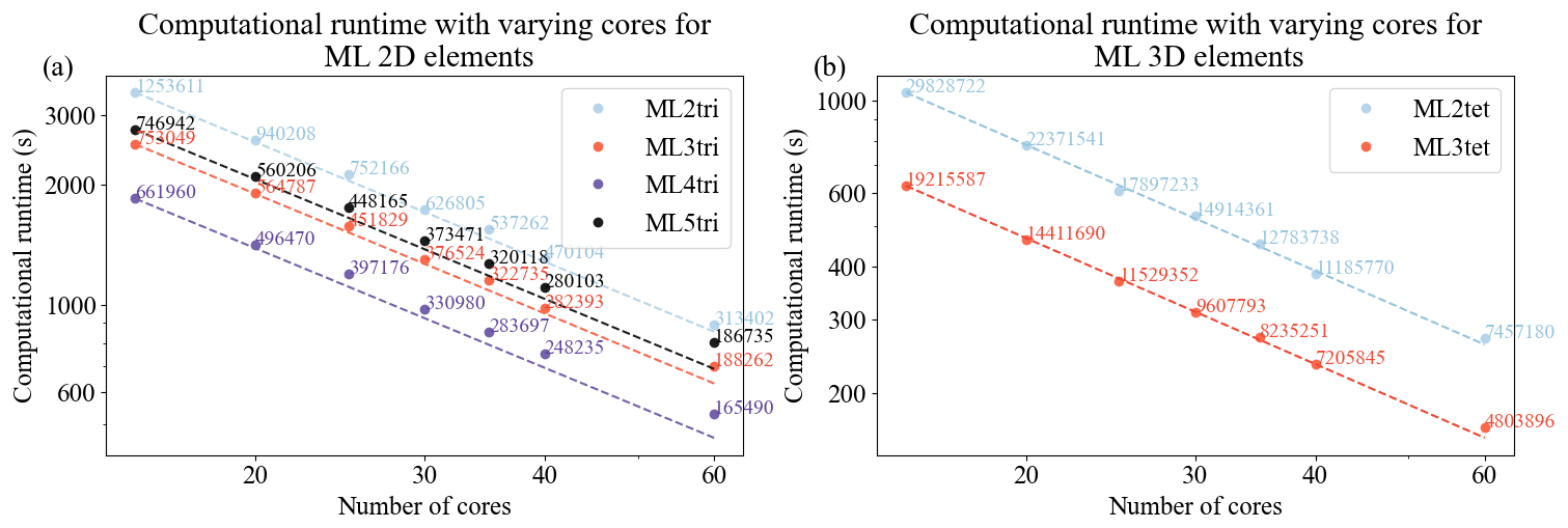
Figure 14 Strong scaling curves for solving the acoustic wave equation with a PML in spyro for 2D (a) and 3D (b) cases given a range of computational resources using Intel nodes. The dashed lines represent ideal scaling for each element, and the average number of degrees of freedom per core is annotated.

The parallel efficiency of our forward propagator was assessed in Intel-based CPUs (see Fig.  14). For the 2D benchmark, the domain contains a uniform velocity of 1.43 km s⁻¹ and spans a physical space of 114 km by 85 km. The 2D domain was discretized using the homogeneous cell densities from Table 2, resulting in 18 804 171, 11 295 747, 9 929 409, and 11 204 136 DoFs for ML2tri, ML3tri, ML4tri, and ML5tri, respectively. In addition to the physical domain, a 0.287 km wide PML was included on all sides of the domain except the free surface. A source term with a time-varying Ricker wavelet that had a central frequency of 5.0 Hz was injected into the domain, and a line of 15 receivers with offset varying from 2.0 to 10.0 km recorded the solution. The 2D simulations were executed for 4.0 s with a time step of 0.5 ms.

The 3D domain was 8 km by 8 km by 8 km with an additional 0.287 km wide PML included on all sides of the domain except the free surface. The domain was discretized using cell densities calculated in Sect. 5.2.4, resulting in 447 430 835 and 288 233 805 for ML2tet and ML3tet, respectively. A source term with a time-varying Ricker wavelet that had a central frequency of 5.0 Hz was injected into the domain, and a cubic grid of 216 receivers was placed with a 2.86 km offset. The 3D simulations were executed for 1.0 s with a time step of 0.5 ms.

Overall, nearly ideal strong scaling was observed in both 2D and 3D cases for most of the elements tested up to 60 computational cores. Since the ML elements admit diagonal mass matrices that avoid the need to solve a linear system, additional MPI communication is circumvented, which greatly improves parallel scalability. We point out that this analysis considers the grid-point-per-wavelength results when designing the mesh sizes and thus represents a practical workload configuration. Weak scaling is also observed out to an average of 165 490 DoFs in 2D and 4 803 896 DoFs using 60 cores. With that said in 2D, scaling deviates somewhat from the ideal curve for ML4tri between 40 and 60 cores. With 60 cores, the ML4tri features the smallest problem in terms of average number of DoFs per core, and symbolic operations can begin to inhibit parallel scalability. It is important to note that similar parallel performance was also obtained for the adjoint-state wave propagator as it is highly similar in operations to the forward-state propagator.

5.4 Experiment with Marmousi2

To investigate FWI (Algorithm 1) with variable unstructured meshes, several 2D inversions were performed using the Marmousi2 model (Martin et al., 2005) (Fig. 15). The objective of this experiment was to intercompare the performance of FWI in terms of wall-clock time, peak memory usage, and final inverted model. All inversions used meshes with variable elemental resolution based on the results with the homogeneous velocity model detailed in Sect. 5.2.2. The Firedrake programming environment enables us to flexibly select the variable space order at runtime.

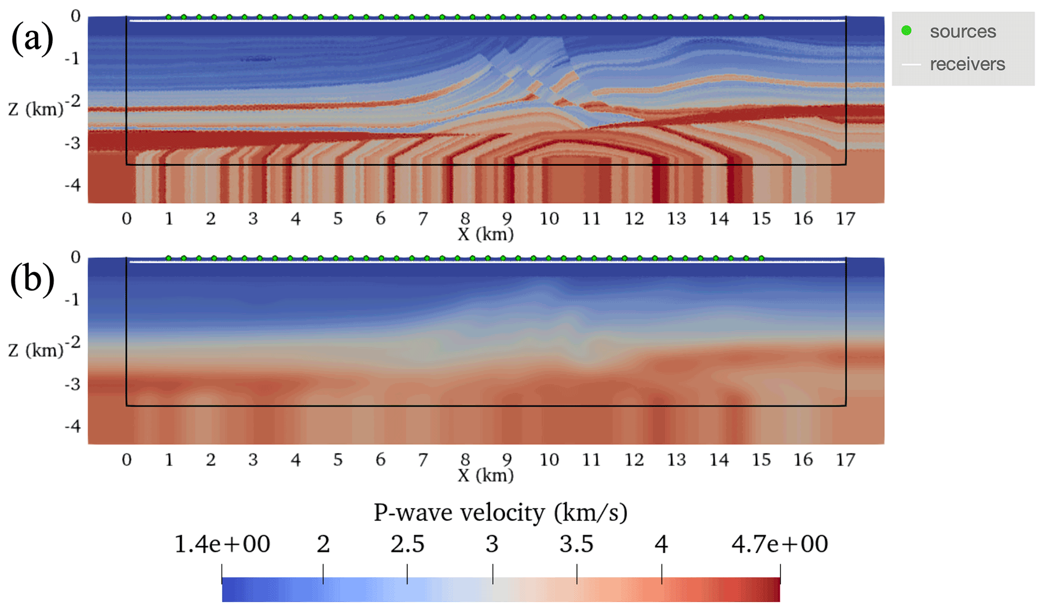
Figure 15 The Marmousi2 model setup described in Sect. 5.4. Panel (a) shows the target model, and panel (b) shows the guess velocity model. On both panels, sources and receivers are annotated. The Ω₀ is the region inside the solid black line.

FWIs commenced from an initial P-wave speed model obtained by smoothing the ground truth Marmousi2 model with a Gaussian blur that had a standard deviation of 100 grid points (Fig. 15a–b). The water layer (i.e., region of the velocity model with P-wave speed <1.51 km s⁻¹) was made exact in the initial seismic velocity model and was fixed throughout the inversion process by setting the gradient to zero there.

Each inversion used an acquisition geometry setup of 40 sources equispaced in the water layer between the coordinates $(-\mathrm{0.01},\mathrm{1.0})$ and $(-\mathrm{0.01},\mathrm{15.0})$ km. A horizontal line of 500 receivers were placed at 100.0 m deep below the water layer between $(-\mathrm{0.10},\mathrm{0.10})$ and $(-\mathrm{0.10},\mathrm{17.0})$ km. Simulations were integrated for 5.0 s with a noiseless Ricker wavelet that had a peak frequency of 5 Hz. A PML was added to the domain with a width $c_{\max }/f_{\max }=\mathrm{900}$ m (Kaltenbacher et al., 2013), and the non-reflective boundary was used to suppress free-surface multiplies (Eq. 6).

The FWI setup described in Algorithm 1 was run for a maximum of 100 iterations iter_max=100. Note that an iteration is only counted if it reduces the cost functional. The inversion process was terminated if either (a) the norm of 𝒢 was less than $\mathrm{1}\times {\mathrm{10}}^{-\mathrm{10}}$ or (b) a maximum of five line searches were unable to reduce J. However, neither criterion was reached in this experiment. A lower bound on the control c of 1.0 km s⁻¹ and an upper bound of 5.0 km s⁻¹ were enforced throughout the optimization to ensure the result remained physical. Simulations were executed in serial using a numerical stable time step of 0.001 s with a subsampling ratio r=10, which yields a gradient calculation frequency 10 times less than the Nyquist frequency as determined by the 5 Hz peak source frequency.

Except for the ML1tri experiment, all meshes for the initial velocity model were generated using the C from Table 2 with an additional 20 % to take into account the heterogeneous velocity model of Marmousi2 Table 3. It is general practice to increase the C for heterogeneous velocity models (Lyu et al., 2020; Anquez et al., 2019). In the case of ML1tri, the only possible mesh configuration that was capable to maintain the threshold error below 30% was C=20. The so-called ground truth shot records that were used to drive the inversion process were simulated with a separate mesh discretized using the ground truth velocity model (see Figure 15a) with ML5tri elements using C=2.03. Ground-truth-simulated shot records used a smaller time step than what was used in FWI of 2.5 ms to minimize error associated with the time discretization.

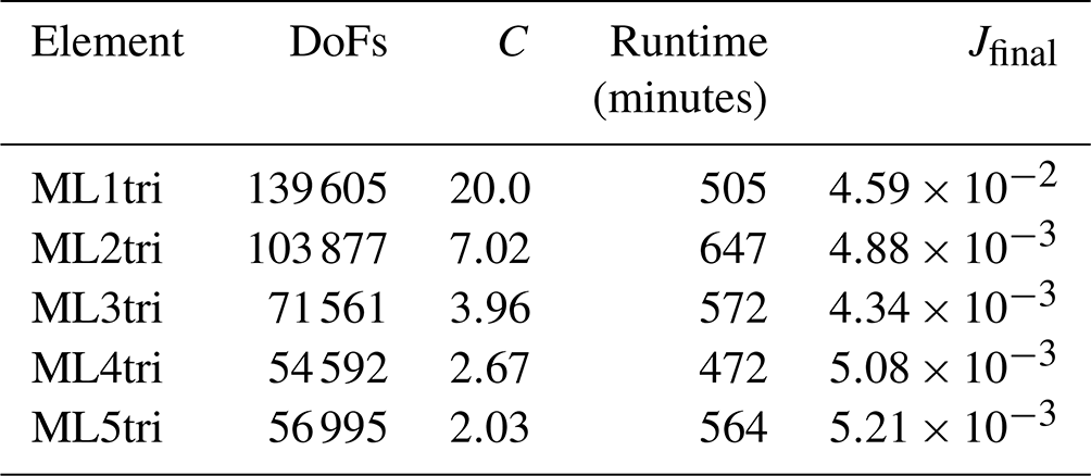
Table 3 The number of degrees of freedom (DoFs) for each experiment, the cells per wavelength C used to generate the mesh, the total wall-clock time to run each FWI discretized with a different element type, and the final cost functional J_final.

The simulations were performed using one shot per core using the shot-level ensemble parallelism described in Sect. 5.3 with 40 computational cores of one Intel node. Throughout each inversion, the total random access memory (RAM) as a function of iteration, the total wall-clock time spent performing the inversion, the cost functional J (Eq. 10) at each iteration, and the total number of iterations were recorded and documented.

5.4.1 Results

The number of DoFs varied by approximately a factor of 2 over the range of ML elements tested. As expected, the ML1tri produced the largest problem size with 139 605 DoFs, whereas ML4tri produces the smallest problem size with 54 592 DoFs. Note that all discretizations used a ΔC=20.0% (Eq. 41) to take into account heterogeneity in the velocity model. It is interesting to point out that ML5tri had a greater number of DoFs in the problem than ML4tri despite containing both higher-order basis functions and a lower C. We also note that in spite of going up to ML5tri, the variable mesh resolution enabled all FWIs to be simulated at a 1 ms time step.

The final inverted models are shown in Fig. 16 and are qualitatively highly similar to each other. Given that all forward discretizations were constructed with the same tolerance for E, this is to be expected. All experiments exhibited between 6 and 11 failed line searches during the course of the 100 iterations demonstrating no clear dependence between the number of failed line searches and the element type. With the exception of ML1tri, all results converged to a similar final cost functional between $\mathrm{4.88}\times {\mathrm{10}}^{-\mathrm{3}}$ and $\mathrm{5.21}\times {\mathrm{10}}^{-\mathrm{3}}$ after exhausting the iteration set. As compared to the other FWIs, the final cost functional for ML1tri was largely greater by an order of magnitude ($J=\mathrm{4.59}\times {\mathrm{10}}^{-\mathrm{2}}$), but still the inverted velocity model for ML1tri qualitatively resembled the true velocity model.

The total runtime memory and wall-clock varied substantially (Fig. 17, Table 3). For example, ML4tri produced the fastest FWI result completing in 472 min, whereas in comparison ML2tri produced the slowest result of 647 min. There was also a marked increase in total wall-clock time going from ML1tri to ML2tri. Wall-clock runtimes are primarily a result of right-hand side assembly time since solving the linear system with ML elements is pointwise division. Furthermore, the higher k degree results in more shared nodes per element leading to more memory access and slower performance per DoF, which offsets the performance gains from reducing the problem size with variable mesh resolution. In regard to virtual memory usage, however, there was a clear reduction in the peak random access memory (RAM) when ML elements were used, which was also noted in Lyu et al. (2020). For comparison, the ML1tri element produced a peak RAM of 7.5 GB, whereas ML4tri required the least peak RAM of 3.1 GB. The ML5tri required slightly more than ML4tri with 3.13 GB.

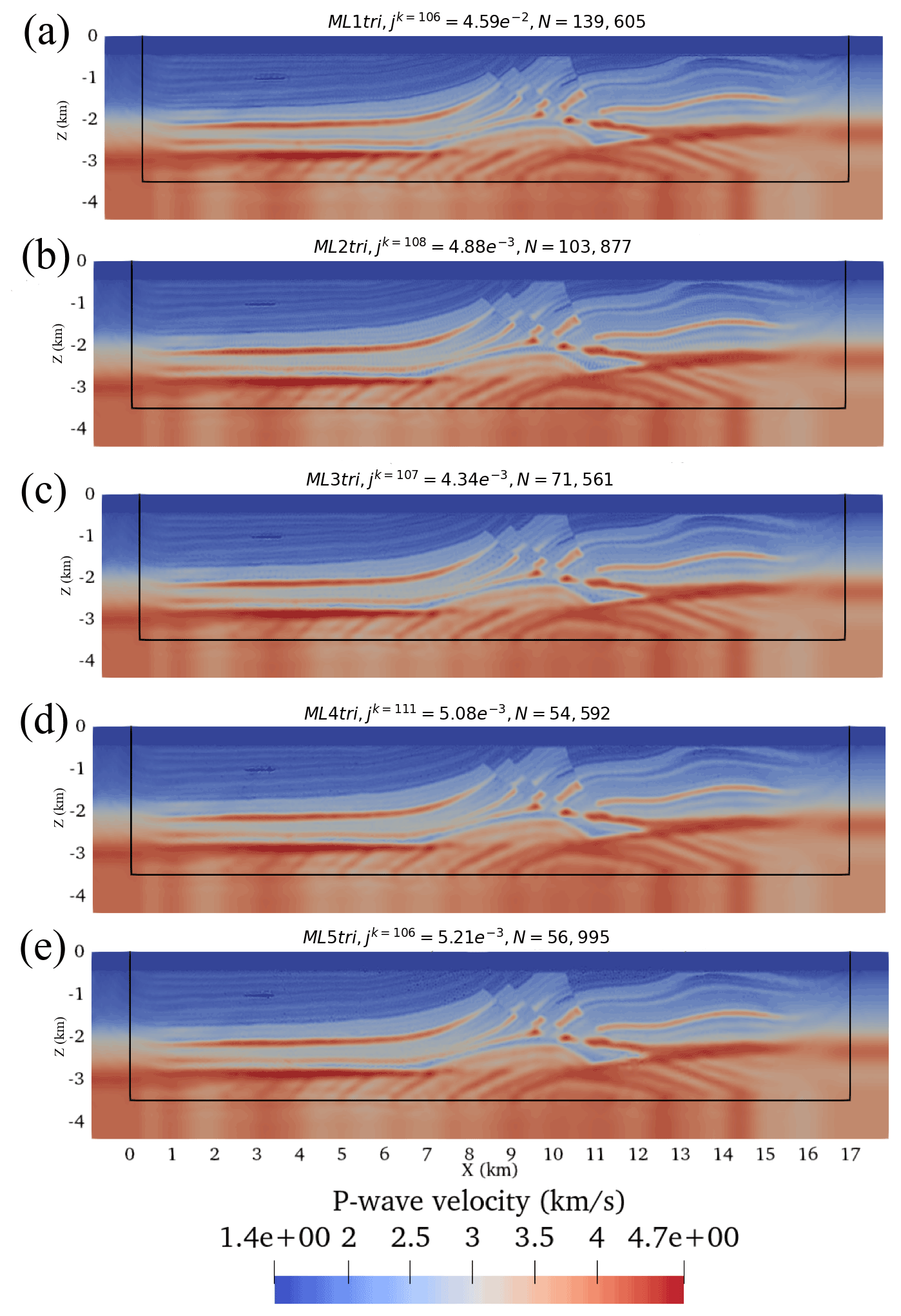
Figure 16 The final result for each FWI using different ML elements. The total number of iterations (including both iterations that reduced the cost functional and the ones that did not) are indicated in each figure along with the final J and number of degrees of freedom N.

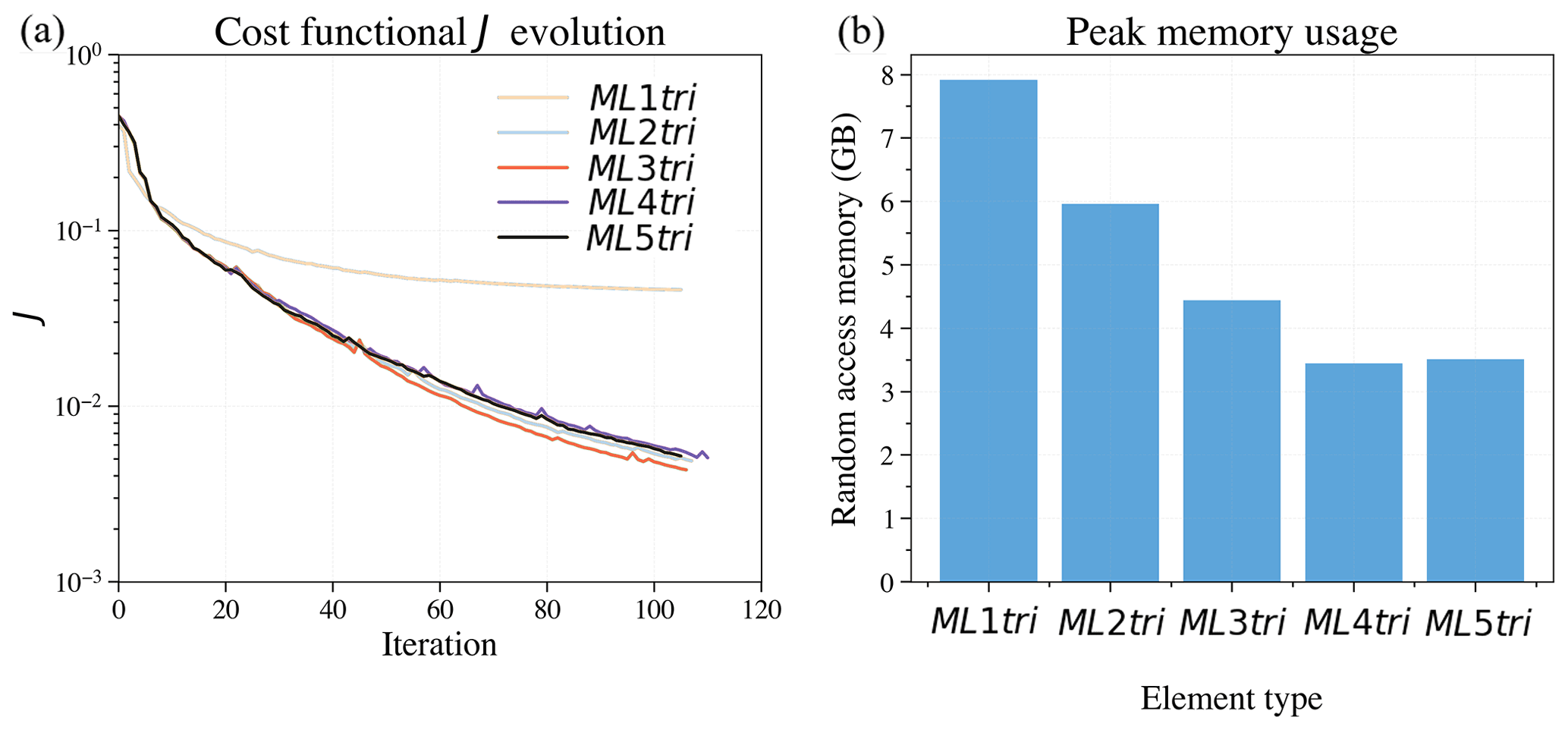
Figure 17 Comparing the performance of FWIs computed with different ML elements. Panel (a) shows the cost functional evolution, and panel (b) shows the peak memory usage.

5.5 Overthrust 3D section

As a demonstration of all the previous developments, the FWI implementation was applied to invert a section of the Overthrust3D P-wave speed model (herein Overthrust3D) (Aminzadeh et al., 1996). Considering that the Overthrust3D is substantial in spatial extent (5.0 km deep × 20.0 m × 20.0 km), the focus of this section is to invert a still considerable 5.175 km by 7.5 km by 7.5 km section of the model (Fig. 18a–b). The initial velocity model used to perform the inversion was obtained by smoothing the true velocity model using a Gaussian kernel with a standard deviation of 100 (Fig. 18b). Similar to the other 2D FWI, the water layer (i.e., region of the velocity model with P-wave speed <1.51 km s⁻¹) was made exact in the guess velocity model and was fixed throughout the inversion process by setting the gradient in the water layer to zero. Finally, a 750 m PML is included on both true and guess models to absorb outgoing waves.

For the inversion, 20 sources were used that were laid out in a 2D grid composed of five lines equispaced along the y axis with each line containing four shots equispaced along the x axis (Fig. 18c). All sources were located at the surface of the domain, and the wave solution was recorded at a 2D grid of 900 receivers laid out 100 m below the surface. Each shot was simulated for 4.0 s, which was sufficient for the wave to spread out through the domain. A 5 Hz noiseless Ricker wavelet was injected at each source location.

Both the guess and true velocity models were discretized with ML3tet elements. Each model featured elements adapted in size to the true and guess model's local seismic velocity given a 5 Hz Ricker wavelet with a C=3.0 that yielded G=6.97 (see Sect. 5.2.4). With this discretization, the guess problem contained 5.3 million DoFs, whereas the true velocity model contained approximately 5.5 million DoFs.

Similar to the 2D FWI experiment, the 3D FWI ran for a maximum of 100 iterations iter_max=100. The inversion process is terminated if either (a) the norm of 𝒢 was less than $\mathrm{1}\times {\mathrm{10}}^{-\mathrm{10}}$ or (b) a maximum of five line searches were unable to reduce J; however, neither criterion was reached in this experiment. A lower bound on the control c of 1 km s⁻¹ and an upper bound of 6 km s⁻¹ were enforced throughout the optimization to ensure the result remained physical. A numerical time step of 0.75 ms was utilized, and a gradient subsampling rate of r=20 was used to conserve memory.

Simulations were performed using the two-level parallelism strategy with two AMD nodes. Each AMD-based node had an AMD EPYC 7601 machine with 64 cores clocked at 2.2 GHz with 512 GB of RAM. Specifically, each of the 20 shots used 6 cores for spatial parallelism requiring in total 120 computational cores.

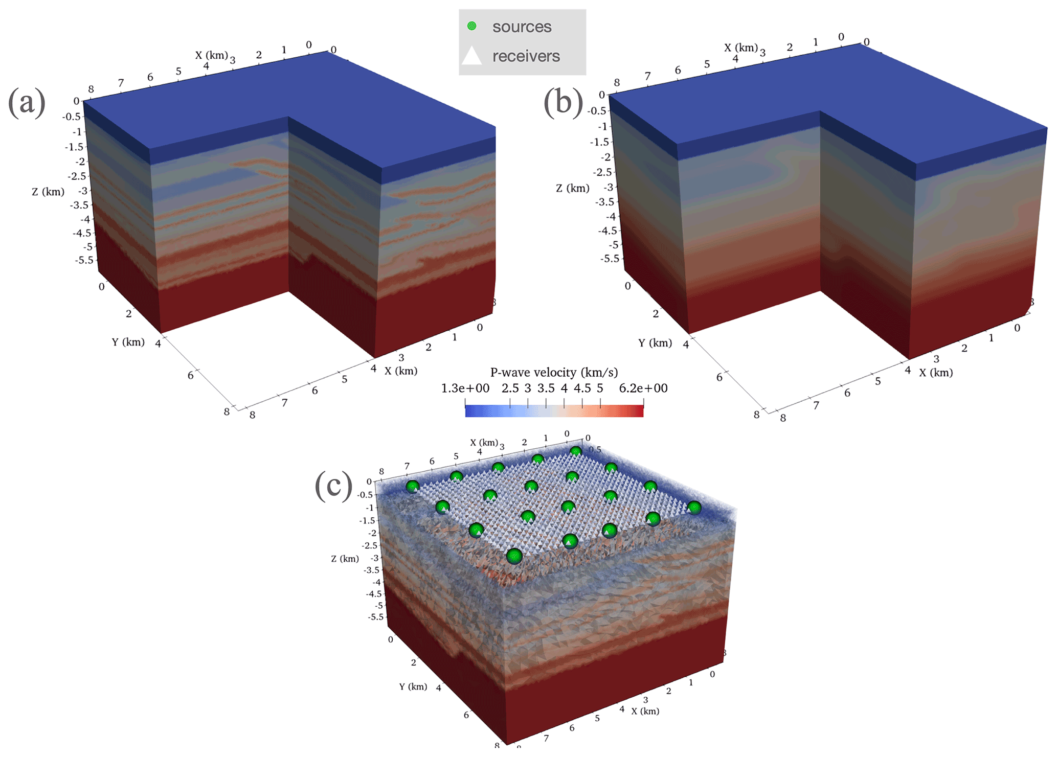
Figure 18 The Overthrust3D setup described in Sect. 5.5. Panel (a) shows the true model, and panel (b) shows the initial model. Panel (c) shows the location of sources and receivers.

5.5.1 Results

The final inversion results along several cross-sectional slices along the x axis and y axis are compared with the true and guess velocity model (Figs. 19 and 20). Overall, the inverted model demonstrates convergence to the true velocity model. After 100 FWI iterations, the cost functional reduced by nearly 1 order of magnitude, from $\mathrm{4.76}\times {\mathrm{10}}^{-\mathrm{1}}$ to $\mathrm{6.62}\times {\mathrm{10}}^{-\mathrm{2}}$. Stratified layers appeared in the inverted velocity model that match structures and shapes in the true model, which are not present in the initial model. Overall, the inverted result appears more accurate near the surface closer to the sources than with depth. Noise appears in the final inverted model, however, which motivates the use of a regularization scheme in future FWIs. Another issue present in the final model is aliasing artifacts, caused by the large interval between sources of 1750 m. Ideally this interval would be $\mathit{\lambda }/\mathrm{2}$ but can go up to $\mathrm{3}\mathit{\lambda }/\mathrm{2}$ (Brenders and Pratt, 2007), which for this model and source frequency is 653 m.

Even with the use of mass-lumping elements and variable mesh resolution, 3D FWI remains computationally challenging on a relatively small-scale cluster with 120 cores. In this case, each FWI iteration took approximately 4.8 h, leading to a total continuous execution time of 20 d to perform 100 FWI iterations. Peak memory usage was significantly larger than in the 2D case at approximately 200 GB.

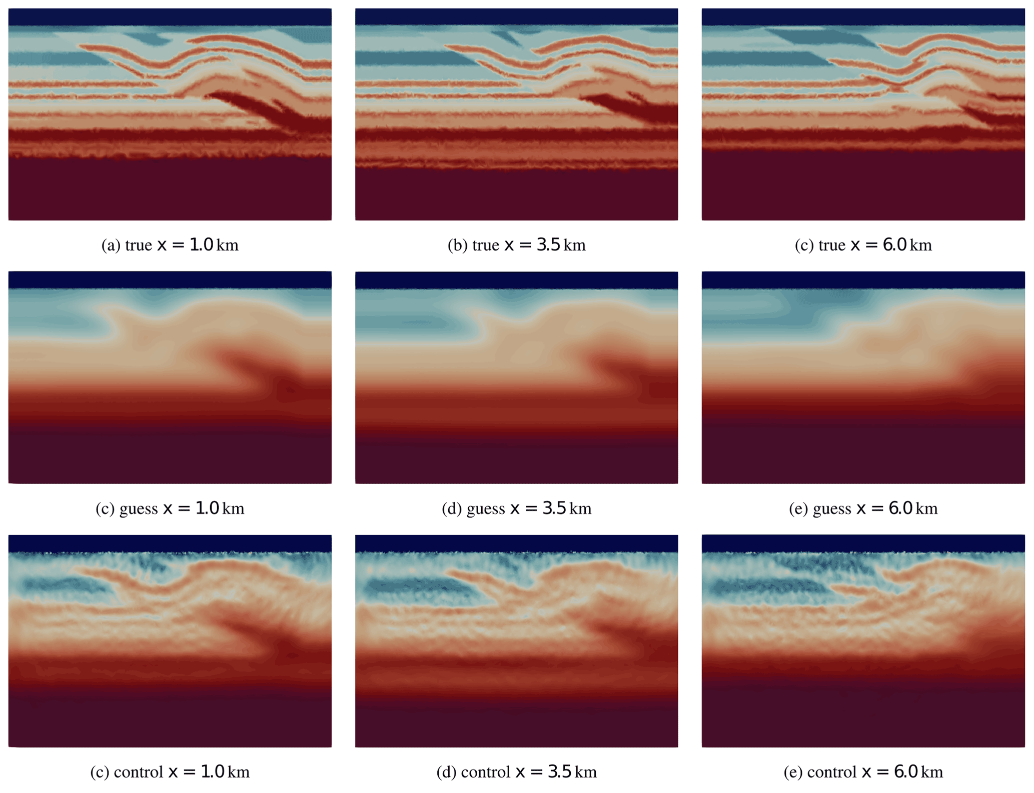
Figure 19 A comparison of cross-sectional slices along the x axis in the Overthrust3D experiment between the true model, guess model, and reconstructed wave field (control) after 100 FWI iterations.

Figure 20 Same as Fig. 19 but for the y axis.

6 Conclusions

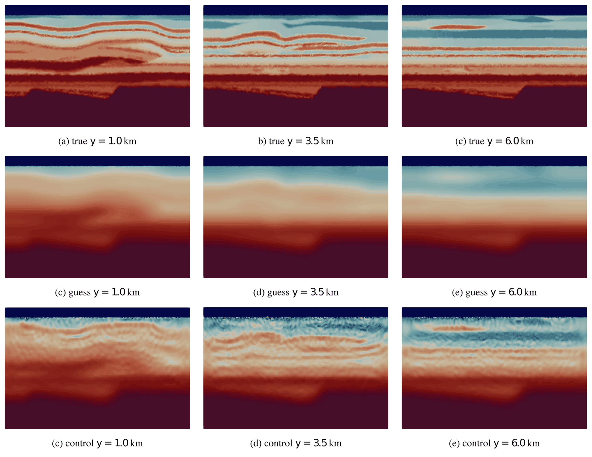
We have discussed a methodology for imaging regional seismic velocity in two- and three-dimensional, arbitrarily heterogeneous, semi-infinite domains in a process commonly referred to as full waveform inversion (FWI). The FWI process involves solving a PDE-constrained optimization problem to minimize the misfit between the collected data and the computed response of the forward equations starting from some initial distribution of seismic velocity. To solve this problem, a continuous Galerkin (CG) finite-element method (FEM) approach was developed using unstructured triangular (i.e., in 2D and tetrahedral in 3D) meshes with elements adapted in size to local seismic velocity. The forward, the adjoint-state wave fields, and the gradient are computed on the same unstructured triangular mesh. The FWI was implemented using the Firedrake package (Rathgeber et al., 2017), which enables us to represent the FEM discretization at a near-mathematical level, simplifying our computer implementation. To solve the optimization problem, the Rapid Optimization Library (ROL; Cyr et al., 2017) was used and called directly from Python using pyROL (Wechsung and Richardson, 2019).

Five triangular 2D elements and three tetrahedral 3D elements that were originally detailed in Chin-Joe-Kong et al. (1999) and Geevers et al. (2018c) (referred to here as ML elements) that yield diagonal mass matrices (mass lumping) with special quadrature rules were implemented inside the Finite Element Automated Tabulator (FIAT, Kirby, 2004). These elements were used to form a fully explicit time-marching scheme for wave propagation with a second-order accurate-in-time scheme. Higher-order ML elements of various orders led to similar final results in a synthetic 2D FWI. As the spatial order increased, we observed a small speedup to perform a fixed number of FWI iterations and a significant reduction in peak memory usage. We also demonstrated that a 3D forward wave simulation could be scaled up in a distributed memory sense with close to ideal strong scalability. To provide practical guidance for subsequent application in FWI, specific mesh resolution requirements were investigated to achieve a fixed error threshold of 5.0 % for 2D/3D forward wave propagation simulations using the ML elements. The usage of higher-order ML elements enabled us to greatly expand the element size while maintaining our desired accuracy. In practical experience, the expansion of the element size can make the removal of degenerate sliver tetrahedral elements far easier, thus encouraging more numerically stable results with larger potentially numerically stable time steps. We highlight that in order to successfully implement FWI with variable-resolution meshes, automated (scripted) mesh generation tools are critically important (e.g., SeismicMesh, Roberts et al., 2021b).

The work presented in this article presents several new directions for FWI with triangular FEM. In the course of the FWI process, the physical model incrementally evolves, and to aid convergence towards the global minimum of the cost function, a multi-scale reconstruction is often used by increasing step by step the frequency of the simulated phenomena. In the case of multi-scale FWI, an automated meshing process in the FWI loop is then crucial to deal with the variations of the physical parameters and the increase of the frequency component of the waves simulated. Waveform-adapted meshes could be used for each frequency of interest so as to obtain an accurate solution while using the coarsest mesh possible.

The current package enables developers to implement forward wave solvers that each make different physical assumptions (variable density acoustic, elastic, visco-elastic, etc.) and discretize them using Firedrake within the current API. In this extensible environment, automatic differentiation (AD) (e.g., dolfin-adjoint, Mitusch et al., 2019) can be used to derive the gradient directly from the forward discretization. We envision future iterations of the package in which the user can readily control the physics and be able to solve more complex, multivariate FWIs without having to focus much effort on repeatedly deriving and implementing adjoint and gradient operators.

Appendix A: Continuous adjoint derivation

In this section, we include a few steps on the continuous adjoint derivation, given in the body of the text in Eqs. (13), (14), and (15), where, for clarity, the formulation will be given for one short only. This is done by differentiating the Lagrangian (Eq. 12) with respect to the forward state, leading to

$$\begin{array}{}\text{(A1)}& \begin{array}{rl}\underset{\mathrm{0}}{\overset{\mathrm{T}}{\int }}\underset{\mathrm{\Omega }}{\int }& {\displaystyle \frac{\partial \mathcal{L}}{\partial (u,\mathit{\omega },\mathbf{p})}}(\mathit{\delta }u,\mathit{\delta }\mathit{\omega },\mathit{\delta }\mathbf{p})=\underset{\mathrm{0}}{\overset{\mathrm{T}}{\int }}\underset{\mathrm{\Omega }}{\int }{\displaystyle \frac{\partial J}{\partial u}}\mathit{\delta }u\\ & +\underset{\mathrm{0}}{\overset{\mathrm{T}}{\int }}\underset{\mathrm{\Omega }}{\int }{u}^{†}\left({\displaystyle \frac{{\partial }^{\mathrm{2}}\mathit{\delta }u}{\partial t^{\mathrm{2}}}}+\mathrm{tr}{\mathrm{\Psi }}_{\mathrm{1}}{\displaystyle \frac{\mathit{\delta }\partial u}{\partial t}}+\mathrm{tr}{\mathrm{\Psi }}_{\mathrm{3}}\mathit{\delta }u+\det {\mathrm{\Psi }}_{\mathrm{1}}\mathit{\delta }\mathit{\omega }\right.\\ & \left.-\mathrm{\nabla }\cdot \left(c^{\mathrm{2}}\mathrm{\nabla }\mathit{\delta }u\right)-\mathrm{\nabla }\cdot \mathit{\delta }\mathit{p}\right)\\ & +\underset{\mathrm{0}}{\overset{\mathrm{T}}{\int }}\underset{\mathrm{\Omega }}{\int }{\mathit{p}}^{†}\cdot \left({\displaystyle \frac{\partial \mathit{\delta }\mathit{p}}{\partial t}}+{\mathrm{\Psi }}_{\mathrm{1}}\mathit{\delta }\mathit{p}+{\mathrm{\Psi }}_{\mathrm{2}}\left(c^{\mathrm{2}}\mathrm{\nabla }\mathit{\delta }u\right)\right.\\ & \left.-{\mathrm{\Psi }}_{\mathrm{3}}\left(c^{\mathrm{2}}\mathrm{\nabla }\mathit{\delta }\mathit{\omega }\right)\right)+\underset{\mathrm{0}}{\overset{\mathrm{T}}{\int }}\underset{\mathrm{\Omega }}{\int }{\mathit{\omega }}^{†}\left({\displaystyle \frac{\partial \mathit{\delta }\mathit{\omega }}{\partial t}}-\mathit{\delta }u\right),\end{array}\end{array}$$

which has to vanish to guarantee the optimality conditions for every trial function $(\mathit{\delta }u,\mathit{\delta }\mathit{\omega },\mathit{\delta }\mathbf{p})$. To do so, we isolate them by performing successive integration by parts, leading to

$$\begin{array}{}\text{(A2)}& \begin{array}{rl}\underset{\mathrm{0}}{\overset{\mathrm{T}}{\int }}\underset{\mathrm{\Omega }}{\int }& {\displaystyle \frac{\partial \mathcal{L}}{\partial (u,\mathit{\omega },\mathbf{p})}}(\mathit{\delta }u,\mathit{\delta }\mathit{\omega },\mathit{\delta }\mathbf{p})=\underset{\mathrm{0}}{\overset{\mathrm{T}}{\int }}\underset{\mathrm{\Omega }}{\int }\mathit{\delta }u{R}_u^{†}(u^{†},{\mathit{p}}^{†},{\mathit{\omega }}^{†})\\ & +\underset{\mathrm{0}}{\overset{\mathrm{T}}{\int }}\underset{\mathrm{\Omega }}{\int }\mathit{\delta }\mathbf{p}\cdot R_{\mathit{p}}^{†}(u^{†},{\mathit{p}}^{†},{\mathit{\omega }}^{†})+\underset{\mathrm{0}}{\overset{\mathrm{T}}{\int }}\underset{\mathrm{\Omega }}{\int }\mathit{\delta }\mathit{\omega }{R}_{\mathit{\omega }}^{†}(u^{†},{\mathit{p}}^{†},{\mathit{\omega }}^{†})\\ & +\underset{\mathrm{\Omega }}{\int }{\left(-{\displaystyle \frac{\partial \mathit{\delta }u}{\partial t}}{u}^{†}+\mathit{\delta }u({\displaystyle \frac{\partial \mathit{\delta }{u}^{†}}{\partial t}}+\mathrm{tr}{\mathrm{\Psi }}_{\mathrm{1}}{u}^{†}+{\mathit{p}}^{†}\cdot \mathit{\delta }\mathit{p}+{\mathit{\omega }}^{†}\mathit{\delta }\mathit{\omega })\right)}_{\mathrm{0}}^{\mathrm{T}}\\ & +\underset{\mathrm{0}}{\overset{\mathrm{T}}{\int }}\underset{\partial \mathrm{\Omega }}{\int }\left(-c^{\mathrm{2}}\mathrm{\nabla }\mathit{\delta }u\cdot \mathit{n}{u}^{†}+(c^{\mathrm{2}}\mathrm{\nabla }{u}^{†}\cdot \mathit{n}+\mathit{n}\cdot c^{\mathrm{2}}{\mathrm{\Psi }}_{\mathrm{2}}{\mathit{p}}^{†})\mathit{\delta }u\right.\\ & \left.-u^{†}\mathit{\delta }\mathit{p}\cdot \mathit{n}-\mathit{n}\cdot \left(c^{\mathrm{2}}{\mathrm{\Psi }}_{\mathrm{3}}{\mathit{p}}^{†}\right)\right).\end{array}\end{array}$$

The first three terms of the last equation represent three different integrals on $\mathrm{\Omega }\times (\mathrm{0},T)$, which vanish for all trial functions if and only if the residuals $R_u^{†}$, $R_{\mathit{p}}^{†}$, and $R_{\mathit{\omega }}^{†}$ vanish, establishing the adjoint Eqs. (13), (14), and (15). The last two terms are related to the initial/final conditions and boundary conditions respectively. Setting them to zero leads to the boundary conditions for the adjoints discussed in the body of the text.

Appendix B: Discretization details for the forward-state and adjoint-state equations

B1 Expressions for the matrices

The expression of the matrices used in the forward discrete problem is

$$\begin{array}{rl}{\mathbb{M}}_u& ={\mathbb{M}}_{\mathit{\omega }}={\mathbb{M}}_p^{x_k}=\underset{\mathrm{\Omega }}{\int }{\mathit{\varphi }}_i\left(\mathbf{x}\right){\mathit{\varphi }}_j\left(\mathbf{x}\right)\mathrm{d}\mathbf{x}{\mathbb{M}}_{u,\mathrm{1}}\\ & =\underset{\mathrm{\Omega }}{\int }\mathrm{tr}{\mathrm{\Psi }}_{\mathrm{1}}{\mathit{\varphi }}_i\left(\mathbf{x}\right){\mathit{\varphi }}_j\left(\mathbf{x}\right)\mathrm{d}\mathbf{x}+\underset{\partial \mathrm{\Omega }}{\int }c\left(\mathbf{x}\right){\mathit{\varphi }}_i\left(\mathbf{x}\right){\mathit{\varphi }}_j\left(\mathbf{x}\right)\mathrm{d}s\\ & {\mathbb{M}}_{u,\mathrm{3}}=\underset{\mathrm{\Omega }}{\int }\mathrm{tr}{\mathrm{\Psi }}_{\mathrm{3}}{\mathit{\varphi }}_i\left(\mathbf{x}\right){\mathit{\varphi }}_j\left(\mathbf{x}\right)\mathrm{d}\mathbf{x}{\mathbb{M}}_{p,\mathrm{1}}^{x_k,x_l}\\ & =\underset{\mathrm{\Omega }}{\int }{\mathit{\psi }}_i\left(\mathbf{x}\right){\mathrm{\Psi }}_{\mathrm{1}}^{k,l}{\mathit{\psi }}_j\left(\mathbf{x}\right)\mathrm{d}\mathbf{x}\\ & \mathbb{K}=\underset{\mathrm{\Omega }}{\int }{c}^{\mathrm{2}}\left(\mathbf{x}\right)\mathrm{\nabla }{\mathit{\varphi }}_i\left(\mathbf{x}\right)\cdot \mathrm{\nabla }{\mathit{\varphi }}_j\left(\mathbf{x}\right)\mathrm{d}\mathbf{x}{\mathbb{D}}^{x_k}=\underset{\mathrm{\Omega }}{\int }{\mathit{\varphi }}_i\left(\mathbf{x}\right){\displaystyle \frac{\partial {\mathit{\varphi }}_j}{\partial x_k}}\mathrm{d}\mathbf{x}\\ & {\mathbb{D}}_{u,\mathrm{2}}=\underset{\mathrm{\Omega }}{\int }\sum _{k,l}{\mathit{\psi }}_i\left(\mathbf{x}\right){\mathrm{\Psi }}_{\mathrm{2}}^{k,l}{\displaystyle \frac{\partial {\mathit{\psi }}_j\left(\mathbf{x}\right)}{\partial x_l}}\mathrm{d}\mathbf{x}{\mathbb{D}}_{\mathit{\omega },\mathrm{3}}\\ & =\underset{\mathrm{\Omega }}{\int }\sum _{k,l}{\mathit{\psi }}_i\left(\mathbf{x}\right){\mathrm{\Psi }}_{\mathrm{3}}^{k,l}{\displaystyle \frac{\partial {\mathit{\psi }}_j\left(\mathbf{x}\right)}{\partial x_l}}\mathrm{d}\mathbf{x},\end{array}$$

where ${\mathbb{M}}_p^{x_k}$ is the diagonal block of matrix 𝕄_p corresponding to each entry on the (two- or three-dimensional) vector P. Also, the indices k,l represent the lines/rows in the matrices ${\mathrm{\Gamma }}_{\mathrm{1},\mathrm{2},\mathrm{3}}$.