the Creative Commons Attribution 4.0 License.
the Creative Commons Attribution 4.0 License.
 | 21 Oct 2022
A Bayesian data assimilation framework for lake 3D hydrodynamic models with a physics-preserving particle filtering method using SPUX-MITgcm v1
Damien Bouffard
Firat Ozdemir
Cintia L. Ramón
James Runnalls
Fotis Georgatos
Camille Minaudo
Jonas Šukys
We present a Bayesian inference for a three-dimensional hydrodynamic model of Lake Geneva with stochastic weather forcing and high-frequency observational datasets. This is achieved by coupling a Bayesian inference package, SPUX, with a hydrodynamics package, MITgcm, into a single framework, SPUX-MITgcm. To mitigate uncertainty in the atmospheric forcing, we use a smoothed particle Markov chain Monte Carlo method, where the intermediate model state posteriors are resampled in accordance with their respective observational likelihoods. To improve the uncertainty quantification in the particle filter, we develop a bi-directional long short-term memory (BiLSTM) neural network to estimate lake skin temperature from a history of hydrodynamic bulk temperature predictions and atmospheric data. This study analyzes the benefit and costs of such a state-of-the-art computationally expensive calibration and assimilation method for lakes.
- Article
(3624 KB) - Full-text XML
-
Supplement
(647 KB) - BibTeX
- EndNote


Lake management is a constantly evolving tradeoff between different conflict of interest. The most obvious is that lakes are easily accessible sources of drinking water but are also the place into which wastewater is ultimately discharged. Lake stakeholders traditionally evaluate the evolution of lakes from in situ observations. While still not widely used for this purpose, previous studies clearly showed the benefit of one- and three-dimensional hydrodynamic models to project different scenarios for the short- or long-term future (Gaudard et al., 2019; Soulignac et al., 2019; Vinnå et al., 2021).
While a number of dedicated monitoring projects already exist for a number of large lakes, operational, fully three-dimensional (3D) models are quite sparse. The most notable is the NOAA Great Lakes Operational Forecast System (GLOFS; Chu et al., 2011; Anderson et al., 2018), which provide comprehensive predictions (water temperature, velocity and level, and ice cover) for all of the Laurentian Great Lakes. Over 25 years, the forecasting service has been continuously improved with better and more sophisticated models. Currently, data assimilation is used for calibration only (Anderson et al., 2018), but there is research toward making it part of the operational mode as well (Ye et al., 2020). Another platform is Meteolakes, which provides short-term water temperature and velocity forecasts for the Geneva, Biel, Zurich, and Greifen lakes in Switzerland (Baracchini, 2019; Baracchini et al., 2020a, b). The platform uses an ensemble Kalman filter to assimilate remotely sensed lake surface water temperature (LSWT), which reduced the mean temperature prediction error by half. An additional benefit of the ensemble filter was a better prediction of mesoscale physical processes such as gyres and upwellings (Baracchini et al., 2020a). However, due to the limitation of the assimilation scheme, only a fraction (≈3.7 %) of the available LSWT images were used.
The purpose of this study is to investigate a novel approach to the data assimilation of highly heterogeneous data using Bayesian inference techniques applied to a 3D hydrodynamic model of Lake Geneva. The model relies on the ensemble affine invariant sampler (EMCEE; Goodman and Weare, 2010; Šukys and Bacci, 2021) to calibrate the distributions of physical model parameters. The EMCEE is a sampler for Markov chain Monte Carlo that is particularly well suited for nonlinear parameters. The advantage of this approach over standard inference methods is that it provides a more informative and accurate parameter estimation, albeit at higher computational expense. To increase the confidence in the sampling algorithm, we used a particle filter method that provides trajectories consistent with the hydrodynamic model (Andrieu et al., 2010; Šukys and Bacci, 2021). In particular, as a substitute to the more well-known Kalman filter and the 4D-Var algorithms, the trajectories themselves are resampled based on their respective observational likelihoods, with the more probable realizations stochastically forming the basis for sequential predictions. Importantly, the filter does not modify the model states (they are only deleted or replicated instead), and therefore, the predictions do not exhibit shocks generated by some data assimilation models.
A proper assimilation of remotely sensed lake surface water temperature (LSWT) requires an estimation of the water surface temperature from the hydrodynamic predictions. Thus, we deploy a bi-directional long short-term memory (BiLSTM) neural network to estimate the skin temperature of the lake and to quantify its uncertainty. The network relies on a 27 h history of hydrodynamic model bulk temperature and atmospheric predictions as inputs for the conversion. The neural network was trained using 16 months of data (the year 2018 and January–April 2020) together with MeteoSwiss COSMO-1 atmospheric model reanalysis and Meteolakes water bulk temperature predictions.
We present the openly available SPUX-MITgcm framework, which integrates the Bayesian inference algorithms of the SPUX package (Šukys and Bacci, 2021) with the hydrodynamics of the MITgcm code (Adcroft et al., 1997) and the trained BiLSTM network. To the best of our knowledge, the data assimilation and particle filtering approach that we propose in this paper has not been previously tested for fully three-dimensional models due to the relatively high computational costs of the model parameter posterior estimation and lack of supporting software. We investigate the viability of this approach and analyze the performance of individual components. The results demonstrate that, while our methodology improves model performance, the framework requires further improvements to become usable for practical applications.
In this section, we describe the available data, the hydrodynamic model, and our data assimilation approach. As data and software reproducibility are essential for more open and accessible research, in the Supplement, we provide documentation on accessing and running the numerical model, which enables a full replication of the results (over a short period of time) that we present in this paper.
2.1 Study site
Lake Geneva is the largest freshwater lake in western Europe and is located on the border between France and Switzerland, covering an area of approximately 580 km2, with an average depth of 154 m. Spanning 73 km along its longest axis, and with a maximum width of 14 km, the lake consists of a wider and deeper main portion in the east and a narrow and shallow portion in the west. The water level and discharge rate into the Rhône river are managed by a dam on the western end of the lake. Lake Geneva is predominantly vertically stratified in density due to temperature, although complete mixing does occur every few years. The mountainous nature of the region significantly affects the wind patterns over the lake, with northeast and southwest being the prevalent directions. These wind patterns, along with seasonal variability in light penetration depth, significantly affect the thermal structure of the lake (Bouffard and Lemmin, 2013; Bouffard et al., 2018). As the mean water residence time in the lake is 10 years, the primary factor driving the lakes' dynamics is the atmospheric forcing.
2.2 Hydrodynamic model
We simulate the hydrodynamics of Lake Geneva using the MITgcm (Adcroft et al., 1997) package (tag “checkpoint67q”), which uses the finite volume method to solve the incompressible Navier–Stokes equations under the Boussinesq approximation. Alternative package options were FVCOM (Finite Volume Community Ocean Model; Chen et al., 2006), used by the Great Lakes Environmental Research Laboratory (GLERL), and Delft3D-FLOW (Deltares, 2013), used by Meteolakes. We use a hydrostatic formulation combined with a third-order direct space–time flux limiter advection scheme (Prather, 1986). A nonlinear equation of state by McDougall et al. (2003) is applied with constant salinity. Due to the large size of the lake, the Coriolis force is included. A detailed list of the fixed model parameter values is provided in Table 1.
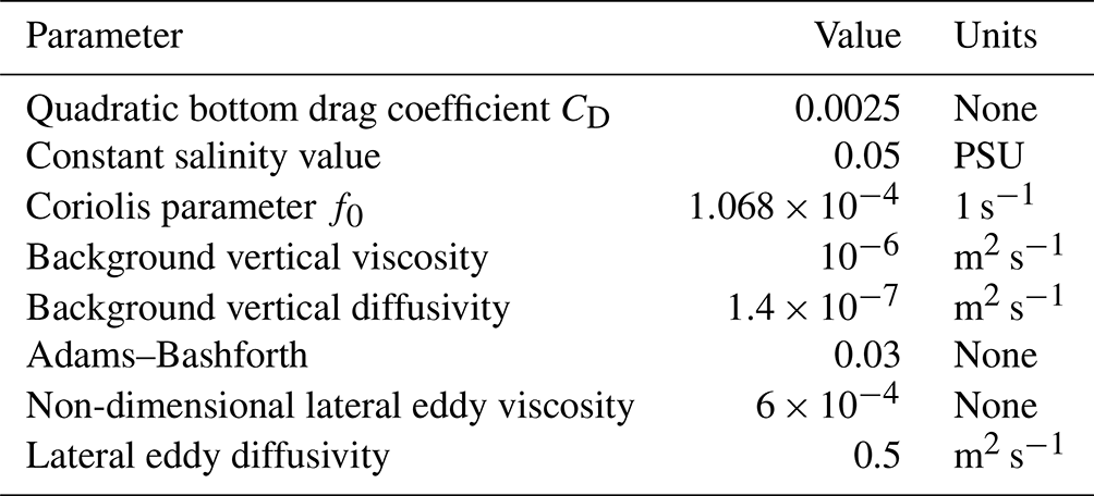
The simulations are performed on a Cartesian grid (z coordinate system), with 1 km horizontal resolution and 50 vertical layers that gradually increase in thickness from 1 m at the surface to 21 m in the deepest portion of the lake. We chose a time step of 60 s. While larger time steps were still numerically stable, a smaller value was helpful in reducing vertical temperature over-diffusion into the deep layers. To improve the accuracy of the topography and reduce spurious artifacts near the bottom, shaved cells are allowed. We apply free-slip boundary conditions to both the horizontal and vertical boundaries and use the non-dimensional bottom drag coefficient from Bouffard and Lemmin (2013) to enable energy dissipation. On the surface, we use an implicit free-surface formulation.
We model the vertical mixing processes using the nonlocal K-profile parameterization (KPP) scheme (Large et al., 1994), which is commonly used in oceanography. Small background vertical diffusivity and viscosity parameters are included to ensure stability (see Table 1). For equivalent parameters on the lateral scales, we manually tuned the eddy viscosity and diffusivity parameters by minimizing the difference between model predictions and in situ temperature profiles at Buchillon station. While a more optimal approach is to infer these parameters, our data assimilation scheme found them difficult to identify (see the Supplement).
Surface forcing inputs were derived from the MeteoSwiss COSMO-E numeric weather prediction model, which are made at 2.2 km resolution. While the COSMO-E model generates an ensemble of 21 predictions, in previous hydrodynamic models of Lake Geneva, only the mean and spread were used (Baracchini et al., 2020b; Cimatoribus et al., 2018). In Sect. 2.4.2, we describe a data assimilation approach that makes use of the individual ensembles which represent the span of weather dynamics more accurately. This approach has the additional advantage of not requiring the estimation of the spatiotemporal noise parameters that Baracchini et al. (2020b) used to add stochasticity to their model. Air pressure, air temperature, wind velocity, longwave radiation, relative humidity, and cloud coverage are used to determine the input fields in accordance with Fink et al. (2014), where the wind drag coefficients of Wüest and Lorke (2003) are used to improve surface stress coupling at low wind speeds. We also include the inflow and outflow of the Rhône river, using the volume flow and temperature measured a few kilometers upstream at Porte du Scex Station (Swiss Federal Office for Environment, FOEN). As smaller tributaries and precipitation/evaporation are not taken into consideration in the model, the water level in the model is manually adjusted to the measured values from the St. Prex station.
Correct transfer of heat and energy from the atmosphere is an essential component of a well-performing hydrodynamic model, especially in summer. In this regard, the bulk transfer coefficient of sensible heat (Dalton number) is a significant parameter that, in several studies (Verburg and Antenucci, 2010; Baracchini, 2019; Rahaghi et al., 2018), has been shown to be larger than the default values used in ocean simulations. Therefore, we seek to infer this parameter. In addition, to more realistically accommodate fluctuations in water transparency, we estimate a spatially uniform Secchi depth using the photosynthetically active radiation (PAR) data from the LéXPLORE moorings (Wüest et al., 2021) to determine the attenuation rate of shortwave energy in the water column. In the future, given the spatial variability in Lake Geneva (Bouffard et al., 2018; Soulignac et al., 2019), a better approach might be to use remote sensing data to estimate the Secchi depth for different lake locations. Finally, we use the albedo formula of Cogley (1979) to account for seasonal changes in surface reflectivity. The Secchi measurements and albedo values are visualized in the Supplement.
2.3 Observational datasets
A particular advantage of the Bayesian framework is the natural ability to handle multiple sources of data with their respective uncertainties. For Lake Geneva, the observations are either in the form of an in situ measurement or remotely sensed surface temperature.
2.3.1 In situ
In situ datasets used in the simulations are summarized in Table 2 and their locations are displayed in Fig. 1. To make the data assimilation process much more manageable, the data from LéXPLORE and FOEN have been subsampled to the hourly rate from the original intervals of 5 s and 10 min, respectively. The vertical resolution of the LéXPLORE dataset was also reduced to match the model discretization levels. Finally, due to the coarse horizontal resolution of the model, only the magnitude of velocity was considered to be a means of calibrating the kinetic energy of the lake.
Table 2Characteristics of the in situ datasets. Note that we assume the FOEN river and water level data to be exact.
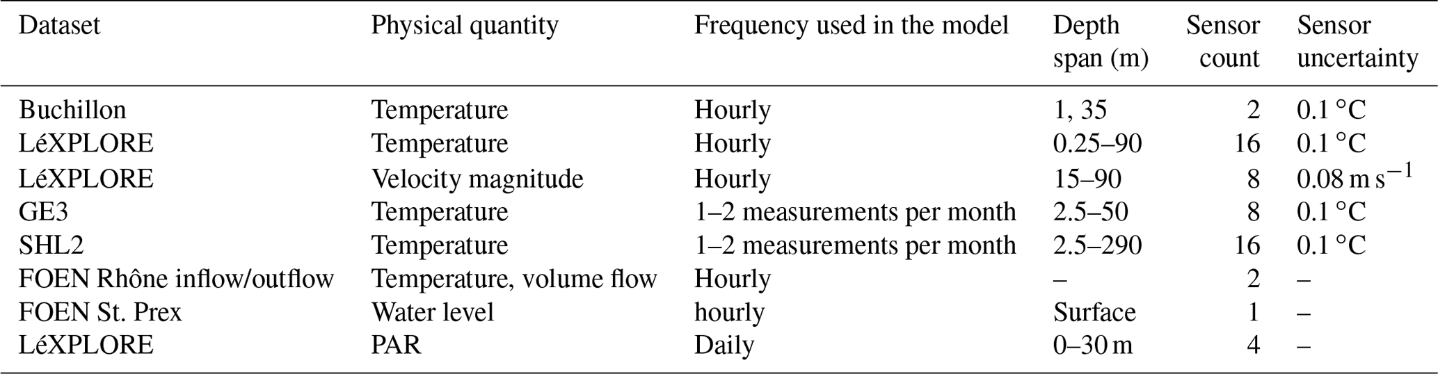
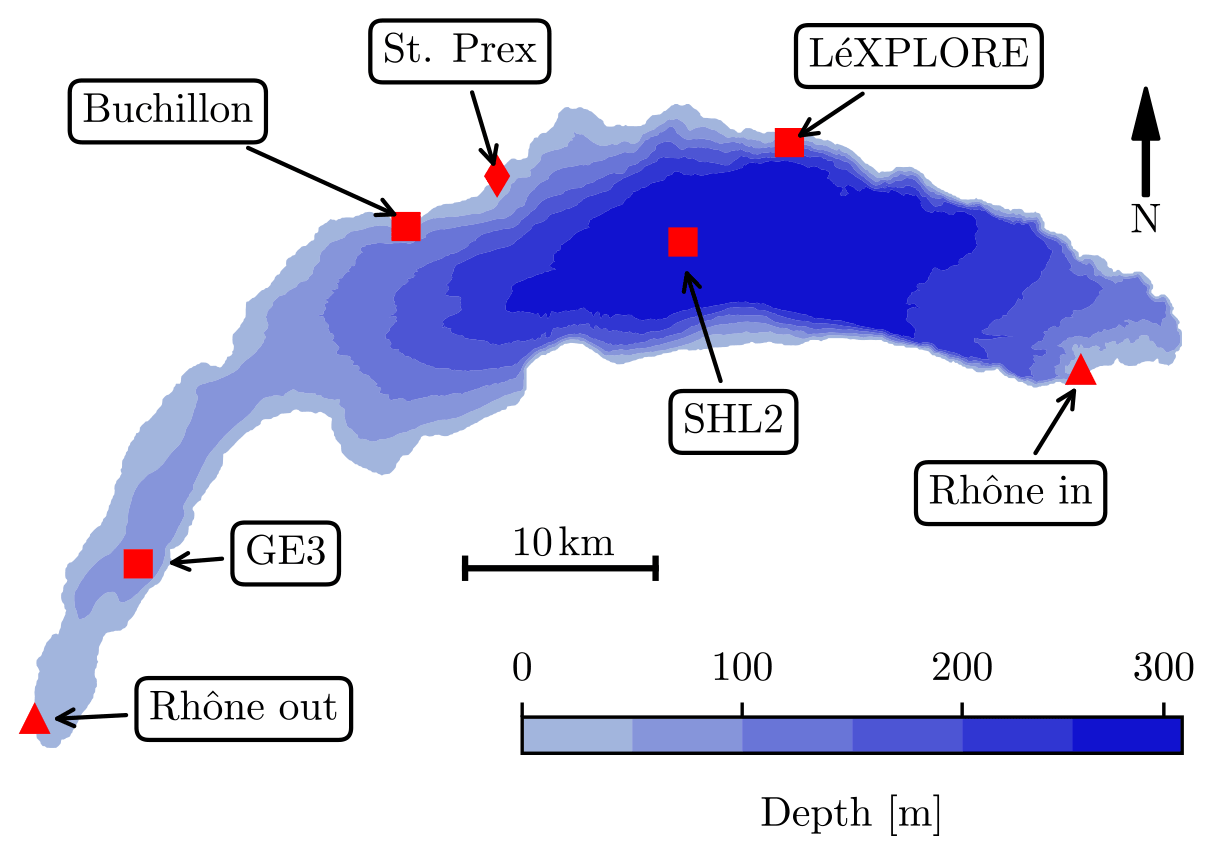
Figure 1Location of the measurement sensors on Lake Geneva. The plot also shows the Rhône inflow and outflow sensor locations and the St. Prex station, which measures the water level.
2.3.2 Remotely sensed temperature
A processing chain from the University of Bern enables the extraction of LSWT images at a resolution of 1 km from the orbital Advanced Very High Resolution Radiometer (AVHRR). On average, typically 10 images of Lake Geneva are generated per day, of which around two are deemed usable by the retrieval process. The quality of an individual snapshot is affected by a number of factors, such as the zenith angle, cloudiness, or sensor errors (Riffler et al., 2015; Kilpatrick et al., 2001). In Lieberherr and Wunderle (2018), a system of assigning a quality flag (QF) for the different satellite measurement conditions was developed. An analysis based on in situ lake data provided an estimate of the uncertainties and biases, ranging from 1.3 ∘C for QF 6 to 1.5 ∘C for QF 1. However, we believe that a more accurate uncertainty model can be established, and therefore, in Sect. 2.4.3, we detail an alternative approach based on machine learning that uses a history of model predictions and weather conditions to generate a bulk-to-skin estimate together with the associated uncertainty.
2.4 Data assimilation
Lakes, akin to the atmosphere, are highly volatile and sensitive systems. For hydrodynamic models, this means that small perturbations in models states can significantly alter the resulting trajectories. Due to the multiple sources of uncertainty present in numerical discretization models, most importantly the uncertainty in forcing terms, such trajectory deviations are ultimately unavoidable. The remedy comes in the form of data assimilation (DA), a framework for providing trajectory corrections based on actual observations.
In discussing sources of uncertainty, a distinction should be made between systematic and random errors (Lahoz and Schneider, 2014). Systematic errors (or bias) arise due to the discrepancy between the model and the actual underlying physics it tries to represent. They can be reduced by certain techniques, such as parameter calibration, but typically cannot be eliminated entirely. Random errors, on the other hand, correspond to inherent uncertainties in the input (weather forcing and LSWT are quite noisy, for example). The DA framework we propose in this paper is designed to deal with these two types of error separately – a particular sampler to reduce systematic errors (parameter inference) and a particle filter to mitigate the stochasticity from weather forcing.
2.4.1 Choice of DA model
A variety of DA algorithms have been proposed and deployed in operational settings and offer different performance-to-optimality tradeoffs. The two primary subfields are variational and sequential methods, with some allowing bias correction (Lahoz and Schneider, 2014). In the variational approach, an objective function describing the discrepancy between the model and observations is sought to be minimized. The 4D-Var is the most popular form and offers the capability to transfer information from observed to unobserved regions for nonlinear models. Some of the drawbacks of this approach are the relatively large numerical costs, both for the model and uncertainty, reduced flexibility, and complex implementation of time-dependent parameters (Lahoz and Schneider, 2014; Baracchini et al., 2020b). From the sequential methods, Kalman filters (KFs), which iteratively evolve a forecast together with error covariance matrices, are an optimal approach. As the true KF is expensive due to the cost of computing the covariance matrix in model space, local model linearity is frequently assumed. For high-dimensional systems, this, however, can result in significant errors in the state and covariance estimation.
Significant performance enhancement is enabled through ensemble methods, where a collection of model states Mj is propagated forward in time, and the resulting trajectories enable the estimation of covariance. The trajectories differ as a result of varying stochasticity in the initial conditions or forcing terms. The ensemble KF (EnKF) is an efficient and highly popular sequential scheme, providing greater stability and an easier covariance estimation (Evensen, 1994). The EnKF has successfully been applied to hydrodynamic forecasting of Lake Geneva by Baracchini et al. (2020a), with a 54 % reduction in temperature error in comparison to an unassimilated model. In recent years, the local ensemble transform KF (LETKF) has been tested in a number of weather prediction frameworks with encouraging results (Gustafsson et al., 2018). The assimilation techniques introduced above have the limitation of assuming that uncertainties and model states are Gaussian and that the model is linear (Lahoz and Schneider, 2014). While this assumption is perfectly reasonable for many applications, non-Gaussian observational error and parameter distributions can be problematic for such methods. For higher-resolution models, the traditional approaches of 4D-Var and EnKF have shown declining performance at the convective scale (Gustafsson et al., 2018; van Leeuwen et al., 2019).
In our model, we employ a particle Markov chain Monte Carlo (MCMC) method, which is highly suitable for nonlinear problems (Andrieu et al., 2010; Šukys and Bacci, 2021). The MCMC algorithm is used to infer selected hydrodynamic model parameters (see Sect. 2.4.2), with an ensemble affine invariant sampler (EMCEE) for the parameter acceptance/rejection criterion. A visualization of the process is shown in Fig. 2. The EMCEE sampler is particularly effective for poorly scaled distributions that become well conditioned under affine transformations and can be significantly faster than standard MCMC approaches on highly skewed distributions. A more thorough discussion of the advantages and disadvantages is given in Goodman and Weare (2010). Here, we only provide a brief overview of the mechanism. The EMCEE algorithm initializes with an ensemble of Markov chains (walkers), {Xi}, drawn from a prior probability distribution, Π(x), and split into two subsets, S1 and S2. Their marginal likelihood is estimated as explained in the paragraph below. First, we update all the walkers Xj from S1 using the stretch formula , where Xk is a randomly chosen walker from S2, and Z is a scaling variable. Each proposed update Xj,new is confirmed in accordance with a Metropolis acceptance probability. The next step is to update S2 walkers using the updated S1 elements. We continue alternatively evolving walkers from S1 and S2 until a suitable convergence criterion is met.
For each EMCEE parameter, a particle filter (PF) is deployed to address the stochasticity of the weather predictions. The PF, implemented in Šukys and Bacci (2021), works as follows. For each parameter , we initialize m model states, Mj, and simulate until an observation is reached at time t=t1 (see Fig. 2). At this point, the model simulations are paused, and all particles are resampled (bootstrapped) according to their observational likelihoods. Thus, certain model states will be deleted and replaced by some other state from a different trajectory. The models are propagated using this mechanism until all the data are assimilated. Such a resampling algorithm significantly increases the algorithmic and implementation complexity due to the required destruction and replication of existing particles. However, it also provides an efficient way of sampling intermediate posterior model states. To the authors' best knowledge, this is the first application of such a filtering algorithm to a fully three-dimensional model. A particular benefit of this approach is that the stochasticity from the atmosphere is sufficient to generate trajectories that manage to track the observational data with proper model parameters. This is in contrast to the non-physical correction vector in many other DA schemes that are necessary to nudge trajectories toward the data. Aside from potentially causing instabilities, these latter approaches decrease the confidence in the fidelity of the underlying model, as the correction mechanism potentially also corrects a model deficiency. At the same time, as no model is perfect, the SPUX PF offers limited capability to handle the biases that the sampler does not eliminate. In addition, the strict nature of our PF (model states cannot be modified) significantly limits its performance, and thus, it cannot be expected to outperform the abovementioned established alternatives.

Figure 2A simplified visualization of the data assimilation framework that we use in this paper. The EMCEE sampler proposes 2n walkers (also called chains in SPUX), whose marginal likelihood is then evaluated using the particle filter (PF). The PF resamples trajectories via deletion/replication with respect to their dataset and observational error model.
2.4.2 Implementation using SPUX and design of numerical experiments
For data assimilation and particle filtering, we use the SPUX package (Šukys and Bacci, 2021), a modular framework for parallel Bayesian inference with a user-friendly programming interface. The 3D hydrodynamics package, MITgcm, was modified to allow a Secchi depth value argument for every simulation hour and was built as a shared library to enable interfacing with SPUX using the ctypes package. The ctypes approach, as opposed to launching the model as a subprocess, provided a noticeably faster and more stable performance. During calibration, EMCEE was configured to run with 16 chains distributed over 8 parallel workers, with 10 particles per filter. This required a total of 89 parallel workers (note that nine of these workers are managers that assign tasks but do not run simulations themselves). The simulations were run at the Swiss National Supercomputing Center (CSCS) over a period of approximately 3 months (≈10.5 h to predict 11 months using the PF and ≈21 h for a full EMCEE sampler iteration).
As described in Sect. 2.2, we chose two hydrodynamic model parameters to infer. In both cases, we can establish an interval (a,b) that contains the optimal value, but we otherwise assume a uniform distribution, U, within. The first parameter is the Smagorinsky harmonic viscosity coefficient Csmag to which we assign a prior distribution U(2,4), consistent with Griffies and Hallberg (2000). To the second parameter – the Dalton number, CD – we assign the prior U(0.045,0.06) based on a preliminary sensitivity analysis. For Dalton values outside the prior, heat exchanges with the atmosphere were not modeled satisfactorily. For example, the default MITgcm value CD=0.0346 results in a significant temperature underprediction during the summer months.
Observational data spanning 15 January–15 December 2019 are used for the calibration and data assimilation (DA) run. Attempts to calibrate the model parameters using a shorter timeframe generated posteriors that provided suboptimal performance for the whole year (see the Supplement for more of a discussion) and was therefore discarded. To analyze the effectiveness of model predictions, a control run (CR) is made without filtering and using parameters CD=0.045 and Csmag=2 as the baseline.
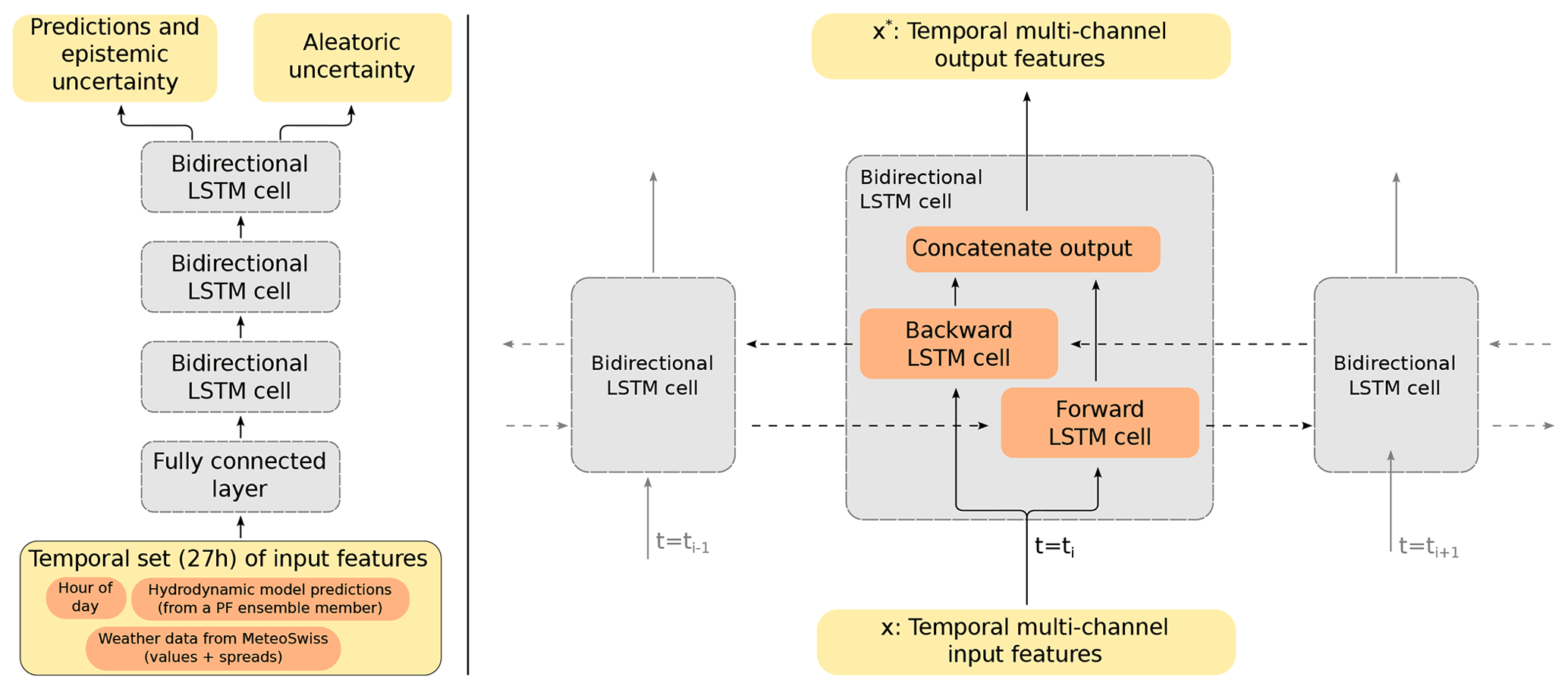
Figure 3A diagram of the neural network we use in our model. On the left, we show the general processing of data within the neural network, and on the right, we show a schematic of a BiLSTM cell.
2.4.3 Bulk-to-skin conversion using LSTM
As the AVHRR operates in the infrared portion of the spectrum, it effectively measures the skin temperature in the top few millimeters of the lake. In the bulk region immediately below this surface layer, the temperature can be significantly different due to a number of factors, such as wind and solar radiation (Wick et al., 1996; Alappattu et al., 2017). As the hydrodynamic model generates bulk temperature predictions, a bulk-to-skin function (forward operator) is necessary for the observation space error model. Existing estimates based on oceanographical studies (e.g., Alappattu et al., 2017) do not directly translate to lake research due to the differences in typical weather conditions such as frequent low wind conditions over lakes (Bouffard and Wüest, 2019). For lakes, an accurate bulk-to-skin parametrization would incorporate effects due to convectively driven surface turbulence (Wilson et al., 2013) and more accurate implementation of the air–water gas exchange, especially in the presence of surfactants (Bouffard and Wüest, 2019). While such a parametrization might be possible, it would be technically difficult to implement, and therefore, we attempt a different approach.
Instead, we implement a neural network using bi-directional long short-term memory (BiLSTM) blocks that use the 27 h history of 18 feature inputs to make a skin temperature prediction. In total, 16 of the features come from the means and their respective spreads of the MeteoSwiss weather predictions (air temperature, cloud cover fraction, wind velocity, relative humidity, precipitation, and shortwave and longwave radiation). The last two features are the hydrodynamic model temperature predictions and hour of the day. The model was trained using data from 2018 and 2020, with the bulk water temperature predictions extracted from the Meteolakes model (Baracchini et al., 2020b). Data from 2019 were separated from the training for benchmarking purposes. A schematic of a BiLSTM block and the neural network is shown in Fig. 3. Input to the neural network is provided as a (27 time step, 18 channel) tensor. An initial, fully connected layer maps these 18 channels to 32 channels. The output is then sequentially passed through three separate BiLSTM cell blocks. Finally, the output of the last BiLSTM block is linearly mapped to a two-channel output, which corresponds to temporal predictions of the skin temperature and their predictive log variances. In our experiments, LSTMs were crucial in order to exploit historical patterns in the input features when predicting the skin temperature. In a recent work, an extension of the LSTMs to a spatially dependent model is presented by Stalder et al. (2021).
For the particle filter, the uncertainty quantification of the predicted skin temperature is also necessary. Accordingly, the BiLSTM blocks in our neural network randomly disables 30 % of the LSTM units to induce stochasticity. This allows our model to also implement additional methods to quantify epistemic and aleatoric uncertainty (Kendall and Gal, 2017). The Monte Carlo dropout approximates predictions from an ensemble that can be used to quantify the epistemic uncertainty. On the other hand, using the negative log likelihood of a normal distribution as the objective function in training allows BiLSTM to also estimate the predicted variance that can be used to quantify aleatoric uncertainty. Specifically, for a given input of 18 feature observations over a 27 h history, the neural network predicts the corresponding 27 h skin temperature estimations as well as their estimated logarithmic variances. During the optimization phase of the neural network, the negative log likelihood of a normal distribution from Kendall and Gal (2017) is used, as follows:
where θ are the neural network weights, yi are the observations, and are the skin temperature estimations with corresponding logarithmic variance estimation si. At the test time, we generate model predictions for 19 times for each input, while keeping dropouts within BiLSTMs active, yielding 19 different prediction vectors, similar to an ensemble model. While the mean of the estimated skin surface temperature is used for mean estimates, we use the variance of the 19 predictions for epistemic uncertainty. Aleatoric uncertainty is computed from the predicted variance estimates by taking their average after mapping the predicted logarithmic variance into variance. The total scalar variance is computed as the sum of the two variances. Accordingly, we construct a normal distribution with the computed total variance centered at the mean skin temperature prediction to be evaluated against the LSWT measurement.
In this section, we report on the inference results, with the initial focus on the model parameter inference. As the calibration mechanism operates on distributions, not scalar quantities, the process is more complicated than what is typically done. Therefore, this warrants a closer look at the posterior distributions and diagnostics. Then, we compare the results obtained using the best posterior parameter set, and finally, we evaluate the performance of the BiLSTM network as a predictor of skin temperature.
3.1 Hydrodynamic model calibration
The posterior distribution of two hydrodynamic model parameters (Smagorinsky viscosity and Dalton number) were estimated in SPUX using the EMCEE sampler (see Fig. 2). For each of the 16 parameter sets, the EMCEE sampler updates a parameter in case a better-performing one is found or it is deemed to be stuck (no changes for 10 iterations). The PF is not guaranteed to choose the optimal global trajectory for a parameter set, given the computational constraints and the resetting of stuck chains (Šukys and Bacci, 2021), and therefore, some uncertainty around the optimal parameter value is to be expected. In Fig. 4, we show the evolution of the Markov chain parameters in terms of their means and the 5th–95th percentiles. We can observe from the relative stationarity of the distributions that the convergence to the true posterior distribution was likely achieved. We thus conclude that the optimal model parameters were localized with a sufficiently high degree of confidence.
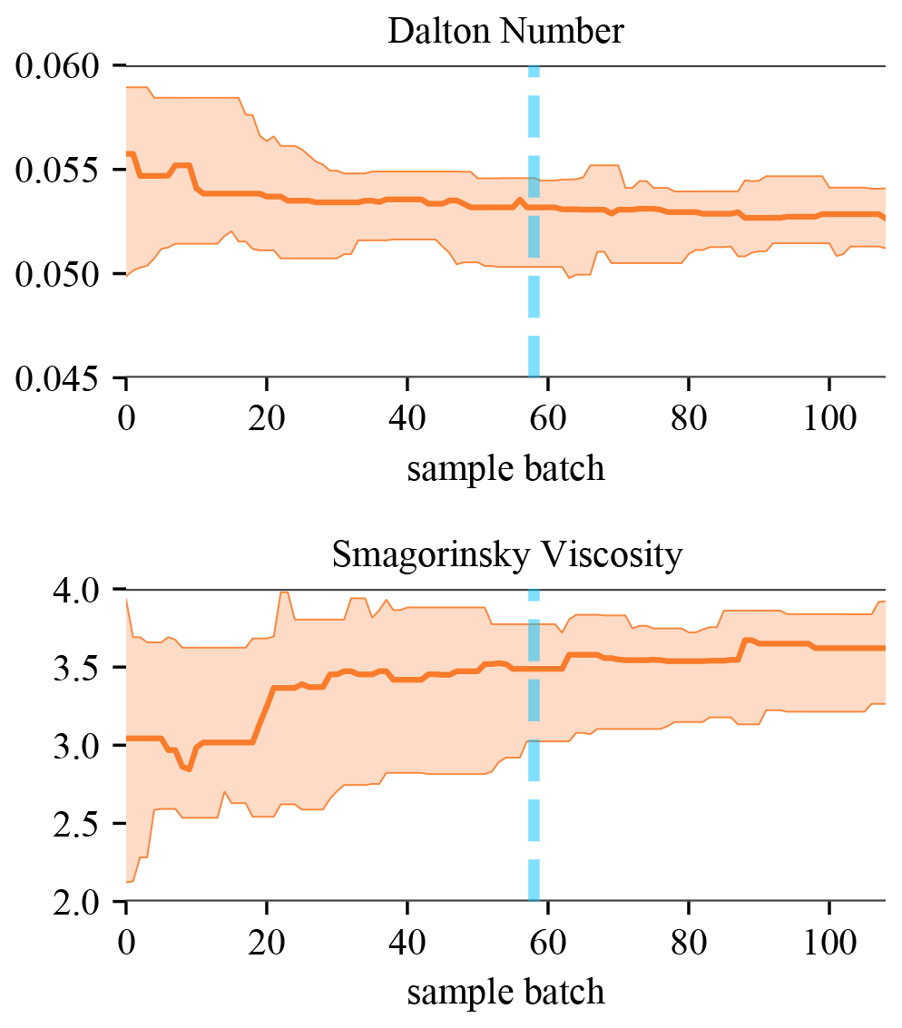
Figure 4Evolution of the 16 Markov chain parameters. The solid lines indicate the median, and the semi-transparent spreads indicate the 5th–95th percentiles across multiple concurrent chains of the sampler. The vertical dashed blue line indicates the end of the specified burn-in period used to determine the posterior distribution.
The inferred marginal posterior distributions are shown in Fig. 5 in orange, with the prior distribution shown in blue. The vertical red dashed lines indicate the best-found parameter set, with the values shown in the table to the right. In relation to their respective priors, the Dalton number is predicted with a relatively high degree of confidence, while the posterior for the Smagorinsky parameter is less defined. This is to be expected as the Dalton number has a stronger effect on model predictions and is therefore more sensitive. However, with more iterations, we expect that a more centered posterior for the Smagorinsky viscosity parameter would have been obtained.
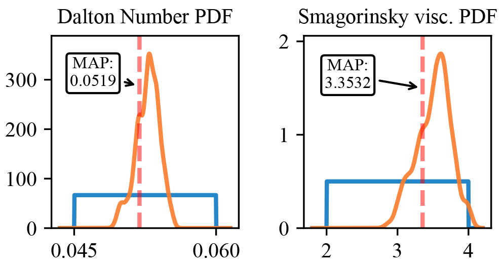
Figure 5Marginal posterior (orange) and prior (blue) distributions of model parameters. The red dashed line indicates the maximum a posteriori parameter (MAP).
We also consider the average redraw rate – the fraction of particles that form a basis for each sequential prediction – in Fig. 6. The survival rates dip significantly in cases when remote sensing data are assimilated or LéXPLORE data are available.
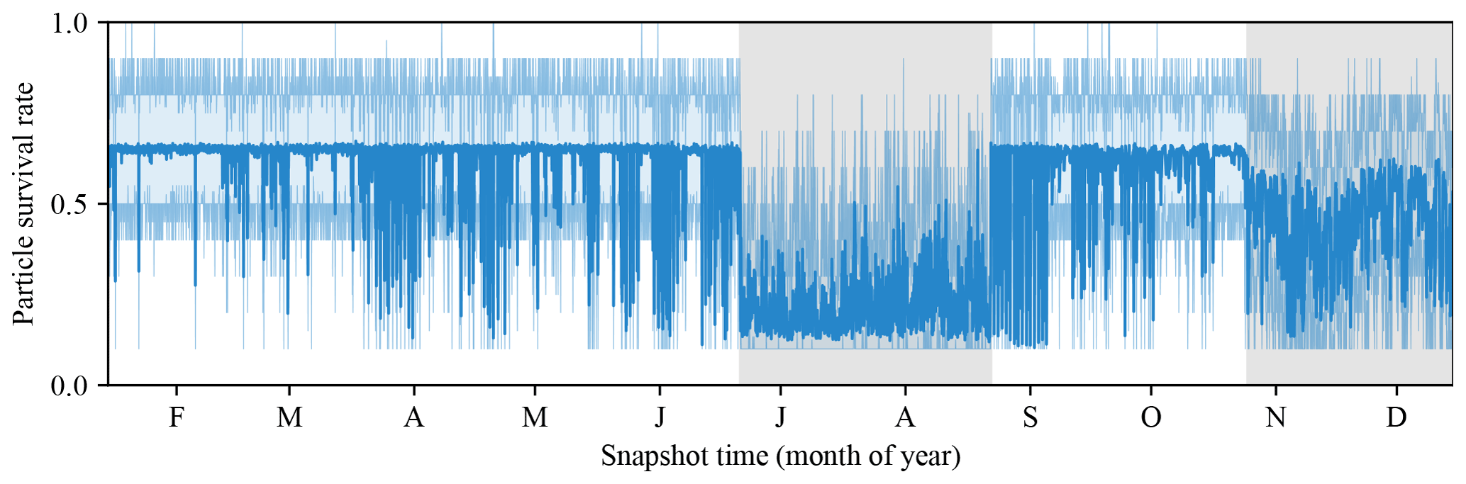
Figure 6Particle survival rates (fraction of particles in the filter that are retained for continuing the DA) for each snapshot time in the PF likelihood estimator. The solid line indicates the mean, and the semi-transparent lines indicate the 0th–100th percentiles. The periods of time when LéXPLORE data are available are shown as shaded gray regions.
3.2 In situ data assimilation results
We present the results of the assimilated data predictions in this section, with the control run (CR) serving as the baseline for comparison. The data assimilation (DA) prediction was generated using the MAP values, which are given in Fig. 5 on the right. In addition, whenever possible, we compare the aggregate error metrics to the values given in Baracchini et al. (2020b) for their 2017 data (specifically, we do not use their 2019 data which exhibit a noticeable drift in the deeper layers of the lake in comparison to SHL2 observations). The performance of the model for the Buchillon, SHL2, and LéXPLORE in situ datasets are considered in this section.
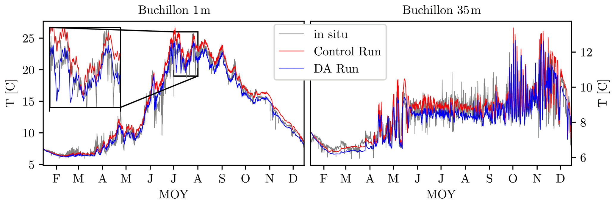
Figure 7Evolution of temperature at the Buchillon station for the 1 m (left) and 35 m (right) sensors for the year 2019. The gray line is the in situ measurement, the red line corresponds to the control run, and the blue line is the data-assimilated prediction. The small inset on the left shows the improvement from the assimilated run for the 1 m sensor in greater detail for July.
Figure 7 shows the temperature for the Buchillon station at depths of 1 m (left) and 35 m (right). The gray lines represent the measurement, the red line shows the CR, and the blue line is the calibrated and data-assimilated (DA) run. As is evident from the results at both depths, the CR already captures the seasonal variation and the high-frequency fluctuations quite accurately. The DA run improves the model performance in the summer, where the CR underpredicts the near-surface temperature, as shown more clearly in the inset which focuses on the predictions for July. For the entire dataset, the root mean square error (RMSE) decreases from 0.95 ∘C for the CR to 0.77 ∘C for the DA run. Overall, the improvement in RMSE and mean average error (MAE) across the various datasets is 4 %–15 % (summarized in Table 3). The main source of the performance improvement is the better resolution of the near-surface temperature in summer.
Table 3Performance of the DA run across the different in situ datasets in comparison to the CR. Note: CR is the control run, DA is the data-assimilated run, RMSE is the root mean square error, and MAE is the mean average error.

We now consider the vertical temperature column profiles from the SHL2 location, which provides monthly measurements at the deepest location in the lake. As both the CR and DA run predictions below 100 m are in agreement with the measurements, we focus on the upper portion of the column. In Fig. 8, we analyze the performance of the models for a few selected snapshots. In Fig. 8, the black dots represent measurements, the dashed red line is the CR, and the thick blue line is the DA run. The results show that the DA run tracks the observed temperature near the surface with greater accuracy, which also results in better modeling of deeper-layer temperature. Below 60 m the observations are followed quite accurately by both the CR and DA run, without any substantial difference between the models.
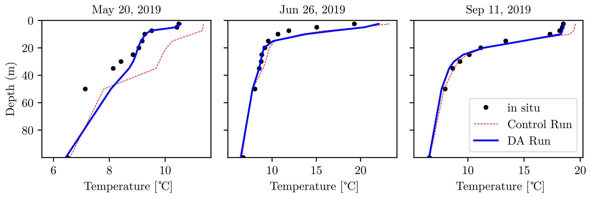
Figure 8Vertical temperature profiles up to 100 m deep at the SHL2 location. The black dots represent observations, the dashed red line is the control run, and the blue line shows the data-assimilated run.
Figure 9 compares the observed vertical column temperature at the LéXPLORE location to the DA run. The vast bulk of measurements for this location (both temperature and velocity) were obtained during two periods, as reflected in the figure. Data for the period 21 June–11 August are shown on the left, and the right side focuses on 25 October until 15 December. For simplicity, we will refer to the respective time intervals as summer and autumn. Outside of those time periods, the measurements were sparse and are therefore omitted from comparison. The results show that the DA algorithm models the water column temperature quite accurately and, in particular, correctly reproduces the thermocline depth in the summer. Furthermore, the cooling cycle at the end of the year is captured quite well. Above the thermocline, the difference plots highlight that the DA run overpredicts the temperature in the summer months, which, as a result, generates a smaller and dissipating warm bias in autumn. The discrepancy could potentially be reconciled with a higher-resolution model or more accurate Secchi depth estimates. In general, correcting temperature overprediction in the subsurface turbulent layer is a difficult problem exhibited in many studies (Cimatoribus et al., 2018; Soulignac et al., 2018; Ye et al., 2020), without a clear consensus on the underlying causes for each case.

Figure 9Vertical temperature profiles from the LéXPLORE sensors for the summer months (left) and late autumn (right). The top row shows the dataset, and the middle row shows the assimilated predictions. The bottom row shows the difference between the plots, with positive values indicating model overprediction.
Due to the coarse horizontal resolution of the mesh, the data assimilation algorithm primarily focused on tracking temperature. As a result, the acoustic Doppler current profiler (ADCP) data played only a secondary role in determining the trajectory of the model. In Fig. 10, we present the kinetic energy spectra computed from the LéXPLORE ADCP data (gray lines) and the DA run (blue lines) based on different datasets. Figure 10 (left), based on summer readings for the 15 m sensor, shows excellent agreement for the kinetic energy variability above the semi-diurnal (12 h) mode. For the same sensor location, model predictions underperform during the autumn (Fig. 10, right), indicating that the high-frequency internal wave modes are not being resolved by the hydrodynamic model. A potentially large contributing factor for the discrepancies is the relatively coarse spatial resolution used in the model.

Figure 10Kinetic energy spectra computed from the ADCP sensors at the LéXPLORE platform (gray) and from the DA run (blue). Profiles based on 15 m deep dynamics use July–August data for panel (a) and November–December data for panel (b).
3.3 LSWT assimilation using BiLSTM network
On average, an LSWT image provided 209 usable pixels and significantly affected particle survival rates. For example, in Fig. 6, most of the low survival rates are due to the AVHRR data, which are especially noticeable in cases when LéXPLORE data are not available. In contrast to Baracchini et al. (2020b), where a highly selective criterion was applied, we use all the pixels which have an associated non-zero QF value. This allowed a much more frequent remote sensing data assimilation, with 798 (of 2092 total) images usable for the data assimilation period. The use of LSWT has enhanced the model predictions by only a 4 % reduction in the in situ RMSE. In Fig. 11, we show an example comparison between the observed LSWT (left), the hydrodynamic model bulk temperature (center), and the BiLSTM prediction (right) for a selected snapshot. The result shows that BiLSTM can predict the spatial variability and structure of LSWT images, although it also frequently generates an entirely different profile. In general, as these improvement results are not particularly informative, we instead focus on the overall performance of the assimilation model and the BiLSTM predictions.
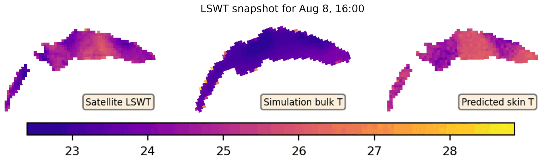
Figure 11A comparison of LSWT snapshot from 8 August 2019 to the DA bulk and BiLSTM skin temperature predictions.
The global training and performance of the BiLSTM model are summarized in Table 4. The training and testing used the means and spreads of the MeteoSwiss weather predictions in combination with Meteolakes mean bulk temperature. The results show that the network significantly improves predictions of LSWT for the training set and achieves a 33 % reduction in RMSE for the test set. In the assimilated run, the bulk prediction difference is already small and only worse than BiLSTM test set performance. In fact, the BiLSTM network increases the RMSE by about 10 %, which is most likely attributable to the differences between the training data and the assimilation process. In general, as LSWT measurements carry significant uncertainty (1.3–1.5 ∘C RMSE), the analytic capability is limited by the lack of exact skin temperature measurements for 2019.
Table 4Results of the BiLSTM model training (left two columns, with bulk temperature from Meteolakes; Baracchini et al., 2020b) and the performance in the DA run (right column).
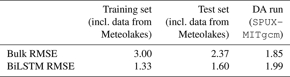
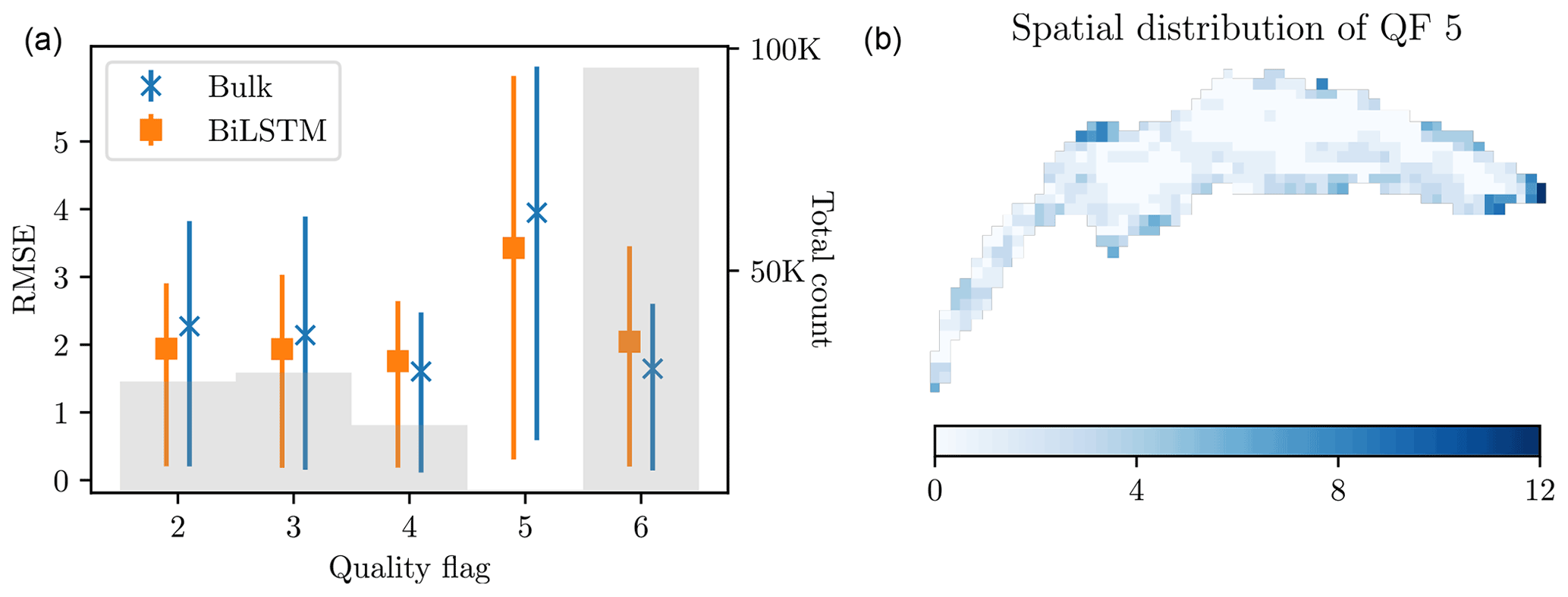
Figure 12Analysis of BiLSTM performance in the DA run with respect to the different quality flags. (a) LSWT difference with respect to bulk temperature (in blue) and BiLSTM predictions (in orange) as a function of QF. The faint gray bars show the total number of LSWT measurements associated with the QF. (b) Spatial distribution of LSWT measurement availability for QF 5.
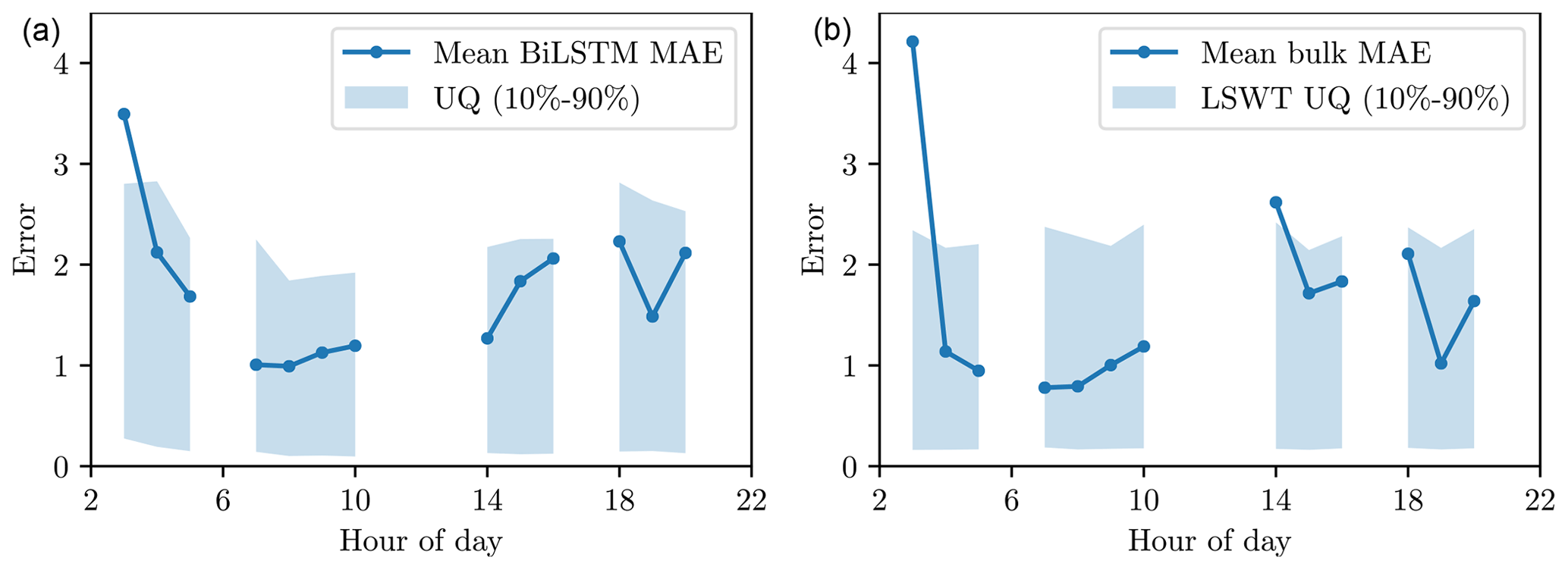
Figure 13(a) Mean BiLSTM prediction error (dark blue line) and the 10th–90th percentiles of the uncertainties predicted by BiLSTM (shaded areas) for the different hours of the day. (b) Mean bulk temperature prediction error (dark blue line) and the 10 %–90 % uncertainty estimates based on Lieberherr and Wunderle (2018).
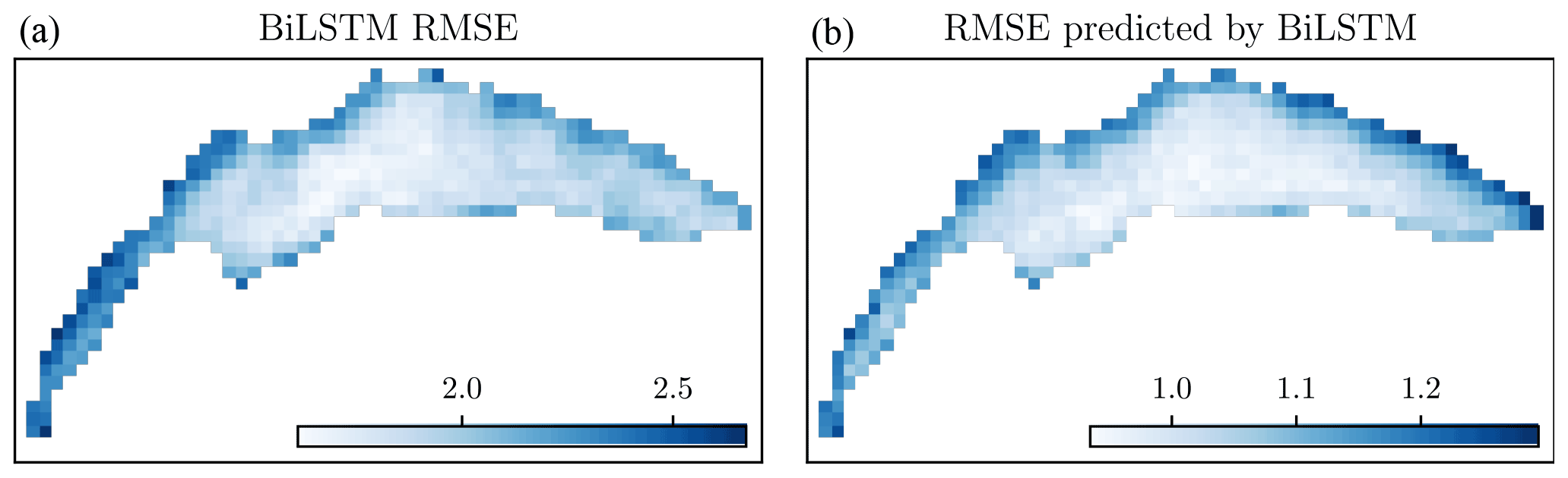
Figure 14Spatial distribution for the BiLSTM RMSE (a) and the RMSE predicted by the BiLSTM (b).
Surprisingly, the predictive capability of the BiLSTM seems to improve for the LSWT pixels with an associated QF in the range 2–5 (42 % of the net pixel count), with an RMSE of 1.92 versus 2.11 ∘C for direct bulk comparison. For the highest quality data (QF 6), however, BiLSTM does not improve the performance. In Fig. 12 (left), we analyze the performance of the BiLSTM (orange lines) against hydrodynamic model bulk predictions (in blue) for the different QFs by plotting the mean RMSE with 10th–90th percentiles. The gray bar chart shows the total number of LSWT measurements for the particular QF level. Aside from QF 5, the bulk RMSE gradually increases for lower QFs, as expected. At the same time, the BiLSTM error is practically constant, with lower uncertainty, indicating the network's capability to predict lower-fidelity data. For QF 5, the discrepancy nearly doubles, indicating a significant issue with this LSWT data subset. In contrast to the relatively uniform spatial frequency of other QFs on the lake, Fig. 12 (right) shows that most of the associated measurements occurred near the shore, which are harder to predict accurately due to the resolution of the hydrodynamic model. However, as LSWT pixels with associated QF 5 are extremely rare (Fig. 12, left), they do not significantly contribute to the overall result.
To enable uncertainty quantification (UQ) for the PF, each individual bulk-to-skin prediction is also equipped with a normal uncertainty distribution, as described in Sect. 2.4.3. Since the network used the hour of the day and weather prediction uncertainty as part of its training, we can expect some spatiotemporal variation in the predicted spreads. Therefore, we analyze those two factors here. In Fig. 13 (left), we show the hourly mean BiLSTM prediction difference with LSTM data as a solid blue line and the 10th–90th percentiles of the BiLSTM UQ as shaded blue regions. The results suggest that neural network UQ is capable of slightly better predicting the spreads for the different times of the day. In contrast, the default LSWT error model provides relatively uniform uncertainties across all times of the day, regardless of the MAE (Fig. 13, right). In general, the improvement is, however, quite mild, potentially due to the low spatial resolution of the model.
Finally, we consider the spatial pattern of BiLSTM predictions and, in particular, examine whether its UQ can predict regions of the lake with larger model discrepancies. In Fig. 14 (left), we present the mean BiLSTM prediction RMSE for the different pixel locations over the lake. As can be expected, the best performance is obtained for offshore pixels in the eastern portion of the lake (Grand Lac). The predictive capability of the network reduces nearshore and especially in the western portion (in the Petit Lac). The BiLSTM uncertainty predictions follow a much similar pattern (Fig. 14, right), including the large increases in uncertainty near the north shores. In part, this increase can most likely be attributed to the greater uncertainty in the atmospheric weather conditions near the land–water interface and the fact that the majority of observations for training BiLSTM come from offshore in the Grand Lac, which would likely create a bias in the model predictions.
We presented the SPUX-MITgcm framework, a novel approach to the calibration of a hydrodynamic model for a highly spatiotemporally heterogeneous observational dataset. The inference makes use of the ensemble affine invariant sampler (EMCEE) to infer the distribution of the model parameters coupled with a particle filter (PF) for stochasticity in atmospheric forcing. The PF relied on resampling existing trajectories, based on their observational likelihoods, to infer the most probable weather conditions over the lake. As a result, the PF generated physically realistic trajectories (at least with respect to the hydrodynamic model). In addition, to enable the proper assimilation of remotely sensed lake surface temperature, we developed a bi-directional long short-term memory network (BiLSTM) for estimating lake skin temperature based on a history of weather and bulk temperature predictions.
The particle filter provides a relatively small improvement to the model predictions (in contrast to other popular data assimilation schemes) but at no cost to the quality of the physical model. However, this approach requires a highly robust hydrodynamic model, as its corrective powers are limited. Despite the improvements, this approach is quite computationally costly, especially as a tool for inferring model parameters. In addition, as discussed in the Supplement, the sampler has significant difficulty with calibrating certain model parameters (although this issue could potentially be mitigated with a better error model). Therefore, we feel that a computationally cheaper method for parameter estimation (for example, an optimization algorithm instead of a sampler) might be the more productive approach. At the same time, an improved version of the particle filtering approach could provide a powerful option for operational forecasting models.
The code used for these simulations, and an example portion of the data, are openly available. The SPUX source code is available at https://doi.org/10.5281/zenodo.5638313 (Safin et al., 2021), the modified MITgcm repository can be found at https://doi.org/10.5281/zenodo.5634042 (Campin et al., 2021), and the repository for handling MITgcm runs is at https://doi.org/10.5281/zenodo.5637216 (Safin, 2021). While we cannot openly publish the forcing data, a representative snapshot is available at https://renkulab.io/gitlab/artur.safin/datalakes-observational-data-snapshot (last access: 30 October 2021), and the 3D mean temperature and velocity predictions can be accessed at https://doi.org/10.5281/zenodo.5642898 (Safin et al., 2019). Finally, the reproducibility of the computational environment is enabled through RENKU (Swiss Data Science Center, 2021), an online platform for the storage, tracking, and replication of numerical codes, which enables users to launch the container directly from the RENKU site. The entire SPUX-MITgcm repository and the computational environment is available as a docker at https://renkulab.io/projects/artur.safin/DatalakesHydrodynamics, and an example of running the inference is in the Supplement.
The supplement related to this article is available online at: https://doi.org/10.5194/gmd-15-7715-2022-supplement.
JŠ and DB designed the research, and AS implemented the data assimilation framework and ran the inference. JŠ extended the SPUX package to be compatible with MITgcm. FO implemented and trained the BiLSTM network. DB and CLR advised with the hydrodynamic model. All authors assisted with discussions, dataset management, and preparation of the paper.
The contact author has declared that none of the authors has any competing interests.
Publisher's note: Copernicus Publications remains neutral with regard to jurisdictional claims in published maps and institutional affiliations.
We would like to thank the entire team from LéXPLORE platform, for their administrative and technical support and for the LéXPLORE core dataset. We also acknowledge the LéXPLORE five partner institutions of Eawag, EPFL, the University of Geneva, the University of Lausanne, and CARRTEL (INRAE-USMB). For SHL2 data, we acknowledge the Observatory on LAkes (OLA), SOERE OLA-IS, AnaEE-France, INRA of Thonon-les-Bains, and CIPEL. We would like to thank the Swiss Federal Office for the Environment (FOEN), for river and water level data, and Stefan Wunderle and the Remote Sensing group at the University of Bern, for LSWT data. The authors would also like to thank Marco Bacci, Theo Baracchini, Fernando Perez-Cruz, Eric Bouillet, and Daniel Odermatt, for helpful discussions.
This work has been funded by the Swiss Data Science Center (SDSC Project DATALAKES C17-17) and Eawag Discretionary Funding.
This paper was edited by Wolfgang Kurtz and reviewed by two anonymous referees.
Adcroft, A., Hill, C., and Marshall, J.: Representation of Topography by Shaved Cells in a Height Coordinate Ocean Model, Mon. Weather Rev., 125, 2293–2315, https://doi.org/10.1175/1520-0493(1997)125<2293:ROTBSC>2.0.CO;2, 1997. a, b
Alappattu, D. P., Wang, Q., Yamaguchi, R., Lind, R. J., Reynolds, M., and Christman, A. J.: Warm layer and cool skin corrections for bulk water temperature measurements for air-sea interaction studies, J. Geophys. Res.-Oceans, 122, 6470–6481, https://doi.org/10.1002/2017JC012688, 2017. a, b
Anderson, E. J., Fujisaki-Manome, A., Kessler, J., Lang, G. A., Chu, P. Y., Kelley, J. G., Chen, Y., and Wang, J.: Ice Forecasting in the Next-Generation Great Lakes Operational Forecast System (GLOFS), J. Marine Sci. Eng., 6, 123, https://doi.org/10.3390/jmse6040123, 2018. a, b
Andrieu, C., Doucet, A., and Holenstein, R.: Particle Markov chain Monte Carlo methods, J. Roy. Stat. Soc. B, 72, 269–342, https://doi.org/10.1111/j.1467-9868.2009.00736.x, 2010. a, b
Baracchini, T.: From observations to 3D forecasts: Data assimilation for high resolution lakes monitoring, PhD thesis, EPFL, Lausanne, https://doi.org/10.5075/epfl-thesis-9475, 2019. a, b
Baracchini, T., Chu, P. Y., Šukys, J., Lieberherr, G., Wunderle, S., Wüest, A., and Bouffard, D.: Data assimilation of in situ and satellite remote sensing data to 3D hydrodynamic lake models: a case study using Delft3D-FLOW v4.03 and OpenDA v2.4, Geosci. Model Dev., 13, 1267–1284, https://doi.org/10.5194/gmd-13-1267-2020, 2020a. a, b, c
Baracchini, T., Wüest, A., and Bouffard, D.: Meteolakes: An operational online three-dimensional forecasting platform for lake hydrodynamics, Water Res., 172, 115-529, https://doi.org/10.1016/j.watres.2020.115529, 2020b. a, b, c, d, e, f, g, h
Bouffard, D. and Lemmin, U.: Kelvin waves in Lake Geneva, J. Great Lakes Res., 39, 637–645, https://doi.org/10.1016/j.jglr.2013.09.005, 2013. a, b
Bouffard, D. and Wüest, A.: Convection in Lakes, Annu. Rev. Fluid Mech., 51, 189–215, https://doi.org/10.1146/annurev-fluid-010518-040506, 2019. a, b
Bouffard, D., Kiefer, I., Wüest, A., Wunderle, S., and Odermatt, D.: Are surface temperature and chlorophyll in a large deep lake related? An analysis based on satellite observations in synergy with hydrodynamic modelling and in-situ data, Remote Sens. Environ., 209, 510–523, https://doi.org/10.1016/j.rse.2018.02.056, 2018. a, b
Campin, J.-M., Heimbach, P., Losch, M., Forget, G., edhill3, Adcroft, A., amolod, Menemenlis, D., dfer22, Hill, C., Jahn, O., Scott, J., stephdut, Mazloff, M., Fox-Kemper, B., antnguyen13, Doddridge, E., Fenty, I., safinenko, Bates, M., Eichmann, A., Smith, T., mitllheisey, Martin, T., Lauderdale, J., Abernathey, R., samarkhatiwala, hongandyan, Deremble, B., and dngoldberg: safinenko/MITgcm: Datalakes-MITgcm (8d98ed1), Zenodo [code], https://doi.org/10.5281/zenodo.5634042, 2021. a
Chen, C., Beardsley, R. C., and Cowles, G.: An Unstructured Grid, Finite-Volume Coastal Ocean Model (FVCOM) System, Oceanography, 19, 78–89, https://doi.org/10.5670/oceanog.2006.92, 2006. a
Chu, P. Y., Kelley, J. G. W., Mott, G. V., Zhang, A., and Lang, G. A.: Development, implementation, and skill assessment of the NOAA/NOS Great Lakes Operational Forecast System, Ocean Dynam., 61, 1305–1316, https://doi.org/10.1007/s10236-011-0424-5, 2011. a
Cimatoribus, A. A., Lemmin, U., Bouffard, D., and Barry, D. A.: Nonlinear Dynamics of the Nearshore Boundary Layer of a Large Lake (Lake Geneva), J. Geophys. Res.-Oceans, 123, 1016–1031, https://doi.org/10.1002/2017JC013531, 2018. a, b
Cogley, J. G.: The Albedo of Water as a Function of Latitude, Mon. Weather Rev., 107, 775–781, https://doi.org/10.1175/1520-0493(1979)107<0775:TAOWAA>2.0.CO;2, 1979. a
Deltares: Delft3D-FLOW user manual, vol. 330, https://content.oss.deltares.nl/delft3d/manuals/Delft3D-FLOW_User_Manual.pdf (last access: 1 May 2021), 2013. a
Evensen, G.: Sequential data assimilation with a nonlinear quasi-geostrophic model using Monte Carlo methods to forecast error statistics, J. Geophys. Res.-Oceans, 99, 10143–10162, https://doi.org/10.1029/94JC00572, 1994. a
Fink, G., Schmid, M., and Wüest, A.: Large lakes as sources and sinks of anthropogenic heat: Capacities and limits, Water Resour. Res., 50, 7285–7301, https://doi.org/10.1002/2014WR015509, 2014. a
Gaudard, A., Råman Vinnå, L., Bärenbold, F., Schmid, M., and Bouffard, D.: Toward an open access to high-frequency lake modeling and statistics data for scientists and practitioners – the case of Swiss lakes using Simstrat v2.1, Geosci. Model Dev., 12, 3955–3974, https://doi.org/10.5194/gmd-12-3955-2019, 2019. a
Goodman, J. and Weare, J.: Ensemble samplers with affine invariance, Commun. Appl. Math. Comput. Sci., 5, 65–80, https://doi.org/10.2140/camcos.2010.5.65, 2010. a, b
Griffies, S. M. and Hallberg, R. W.: Biharmonic Friction with a Smagorinsky-Like Viscosity for Use in Large-Scale Eddy-Permitting Ocean Models, Mon. Weather Rev., 128, 2935–2946, https://doi.org/10.1175/1520-0493(2000)128<2935:BFWASL>2.0.CO;2, 2000. a
Gustafsson, N., Janjić, T., Schraff, C., Leuenberger, D., Weissmann, M., Reich, H., Brousseau, P., Montmerle, T., Wattrelot, E., Bučánek, A., Mile, M., Hamdi, R., Lindskog, M., Barkmeijer, J., Dahlbom, M., Macpherson, B., Ballard, S., Inverarity, G., Carley, J., Alexander, C., Dowell, D., Liu, S., Ikuta, Y., and Fujita, T.: Survey of data assimilation methods for convective-scale numerical weather prediction at operational centres, Q. J. Roy. Meteor. Soc., 144, 1218–1256, https://doi.org/10.1002/qj.3179, 2018. a, b
Kendall, A. and Gal, Y.: What Uncertainties Do We Need in Bayesian Deep Learning for Computer Vision?, in: Advances in Neural Information Processing Systems, edited by: Guyon, I., Luxburg, U. V., Bengio, S., Wallach, H., Fergus, R., Vishwanathan, S., and Garnett, R., vol. 30, Curran Associates, Inc., https://proceedings.neurips.cc/paper/2017/file/2650d6089a6d640c5e85b2b88265dc2b-Paper.pdf (last access: 30 July 2021), 2017. a, b
Kilpatrick, K. A., Podestá, G. P., and Evans, R.: Overview of the NOAA/NASA advanced very high resolution radiometer Pathfinder algorithm for sea surface temperature and associated matchup database, J. Geophys. Res.-Oceans, 106, 9179–9197, https://doi.org/10.1029/1999JC000065, 2001. a
Lahoz, W. A. and Schneider, P.: Data assimilation: making sense of Earth Observation, Front. Environ. Sci., 2, 16, https://doi.org/10.3389/fenvs.2014.00016, 2014. a, b, c, d
Large, W. G., McWilliams, J. C., and Doney, S. C.: Oceanic vertical mixing: A review and a model with a nonlocal boundary layer parameterization, Rev. Geophys., 32, 363–403, https://doi.org/10.1029/94RG01872, 1994. a
Lieberherr, G. and Wunderle, S.: Lake Surface Water Temperature Derived from 35 Years of AVHRR Sensor Data for European Lakes, Remote Sens., 10, https://doi.org/10.3390/rs10070990, 2018. a, b
McDougall, T. J., Jackett, D. R., Wright, D. G., and Feistel, R.: Accurate and Computationally Efficient Algorithms for Potential Temperature and Density of Seawater, J. Atmos. Ocean. Tech., 20, 730–741, https://doi.org/10.1175/1520-0426(2003)20<730:AACEAF>2.0.CO;2, 2003. a
Prather, M. J.: Numerical advection by conservation of second-order moments, J. Geophys. Res.-Atmos., 91, 6671–6681, https://doi.org/10.1029/JD091iD06p06671, 1986. a
Rahaghi, A. I., Lemmin, U., Cimatoribus, A., Bouffard, D., Riffler, M., Wunderle, S., and Barry, D. A.: Improving surface heat flux estimation for a large lake through model optimization and two-point calibration: The case of Lake Geneva, Limnol. Oceanogr.-Methods, 16, 576–593, https://doi.org/10.1002/lom3.10267, 2018. a
Riffler, M., Lieberherr, G., and Wunderle, S.: Lake surface water temperatures of European Alpine lakes (1989–2013) based on the Advanced Very High Resolution Radiometer (AVHRR) 1 km data set, Earth Syst. Sci. Data, 7, 1–17, https://doi.org/10.5194/essd-7-1-2015, 2015. a
Safin, A.: Datalakes-Hydrodynamics. In Geoscientific Model Development (Version v1), Zenodo [code], https://doi.org/10.5281/zenodo.5637216, 2021. a
Safin, A., Runnalls, J., Šukys, J., and Bouffard, D.: Datalakes Observational model predictions (2019), Zenodo [data set], https://doi.org/10.5281/zenodo.5642898, 2021. a
Safin, A., Šukys, J., and Bacci, M.: SPUX-MITgcm (SPUX-MITgcm_v1), Zenodo [code], https://doi.org/10.5281/zenodo.5638313, 2021. a
Soulignac, F., Danis, P.-A., Bouffard, D., Chanudet, V., Dambrine, E., Guénand, Y., Harmel, T., Ibelings, B. W., Trevisan, D., Uittenbogaard, R., and Anneville, O.: Using 3D modeling and remote sensing capabilities for a better understanding of spatio-temporal heterogeneities of phytoplankton abundance in large lakes, J. Great Lakes Res., 44, 756–764, https://doi.org/10.1016/j.jglr.2018.05.008, 2018. a
Soulignac, F., Anneville, O., Bouffard, D., Chanudet, V., Dambrine, E., Guénand, Y., Harmel, T., Ibelings, B. W., Trevisan, D., Uittenbogaard, R., and Danis, P.: Contribution of 3D coupled hydrodynamic-ecological modeling to assess the representativeness of a sampling protocol for lake water quality assessment, Knowl. Manag. Aquat. Ecosyst., 420, 42, https://doi.org/10.1051/kmae/2019034, 2019. a, b
Stalder, M., Ozdemir, F., Safin, A., Šukys, J., Bouffard, D., and Perez-Cruz, F.: Probabilistic modeling of lake surface water temperature using a Bayesian spatio-temporal graph convolutional neural network, arXiv, https://doi.org/10.48550/ARXIV.2109.13235, 2021. a
Šukys, J. and Bacci, M.: SPUX Framework: a Scalable Package for Bayesian Uncertainty Quantification and Propagation, https://arxiv.org/abs/2105.05969, last access: 30 August 2021. a, b, c, d, e, f, g
Swiss Data Science Center: RENKU, https://renkulab.io/, last access: 30 August 2021. a
van Leeuwen, P. J., Künsch, H. R., Nerger, L., Potthast, R., and Reich, S.: Particle filters for high-dimensional geoscience applications: A review, Q. J. Roy. Meteor. Soc., 145, 2335–2365, https://doi.org/10.1002/qj.3551, 2019. a
Verburg, P. and Antenucci, J. P.: Persistent unstable atmospheric boundary layer enhances sensible and latent heat loss in a tropical great lake: Lake Tanganyika, J. Geophys. Res.-Atmos., 115, D11, https://doi.org/10.1029/2009JD012839, 2010. a
Vinnå, L. R., Medhaug, I., Schmid, M., and Bouffard, D.: The vulnerability of lakes to climate change along an altitudinal gradient, Commun. Earth Environ., 2, 35, https://doi.org/10.1038/s43247-021-00106-w, 2021. a
Wick, G. A., Emery, W. J., Kantha, L. H., and Schlüssel, P.: The Behavior of the Bulk – Skin Sea Surface Temperature Difference under Varying Wind Speed and Heat Flux, J. Phys. Oceanogr., 26, 1969–1988, https://doi.org/10.1175/1520-0485(1996)026<1969:TBOTBS>2.0.CO;2, 1996. a
Wilson, R. C., Hook, S. J., Schneider, P., and Schladow, S. G.: Skin and bulk temperature difference at Lake Tahoe: A case study on lake skin effect, J. Geophys. Res.-Atmos., 118, 10332–10346, https://doi.org/10.1002/jgrd.50786, 2013. a
Wüest, A. and Lorke, A.: SMALL-SCALE HYDRODYNAMICS IN LAKES, Annu. Rev. Fluid Mech., 35, 373–412, https://doi.org/10.1146/annurev.fluid.35.101101.161220, 2003. a
Wüest, A., Bouffard, D., Guillard, J., Ibelings, B. W., Lavanchy, S., Perga, M.-E., and Pasche, N.: LéXPLORE: A floating laboratory on Lake Geneva offering unique lake research opportunities, WIREs Water, 8, e1544, https://doi.org/10.1002/wat2.1544, 2021. a
Ye, X., Chu, P. Y., Anderson, E. J., Huang, C., Lang, G. A., and Xue, P.: Improved thermal structure simulation and optimized sampling strategy for Lake Erie using a data assimilative model, J. Great Lakes Res., 46, 144–158, https://doi.org/10.1016/j.jglr.2019.10.018, 2020. a, b