A fast, single-iteration ensemble Kalman smoother for sequential data assimilation

Ensemble variational methods form the basis of the state of the art for nonlinear, scalable data assimilation, yet current designs may not be cost-effective for real-time, short-range forecast systems. We propose a novel estimator in this formalism that is designed for applications in which forecast error dynamics is weakly nonlinear, such as synoptic-scale meteorology. Our method combines the 3D sequential filter analysis and retrospective reanalysis of the classic ensemble Kalman smoother with an iterative ensemble simulation of 4D smoothers. To rigorously derive and contextualize our method, we review related ensemble smoothers in a Bayesian maximum a posteriori narrative. We then develop and intercompare these schemes in the open-source Julia package DataAssimilationBenchmarks.jl, with pseudo-code provided for their implementations. This numerical framework, supporting our mathematical results, produces extensive benchmarks demonstrating the significant performance advantages of our proposed technique. Particularly, our single-iteration ensemble Kalman smoother (SIEnKS) is shown to improve prediction/analysis accuracy and to simultaneously reduce the leading-order computational cost of iterative smoothing in a variety of test cases relevant for short-range forecasting. This long work presents our novel SIEnKS and provides a theoretical and computational framework for the further development of ensemble variational Kalman filters and smoothers.

1 Introduction

1.1 Context

Ensemble variational methods form the basis of the state of the art for nonlinear, scalable data assimilation (DA; Asch et al., 2016; Bannister, 2017). Estimators following an ensemble Kalman filter (EnKF) analysis include the seminal maximum likelihood filter and 4DEnVAR (Zupanski, 2005; Liu et al., 2008), the ensemble randomized maximum likelihood method (EnRML; Gu and Oliver, 2007; Chen and Oliver, 2012; Raanes et al., 2019b), the iterative ensemble Kalman smoother (IEnKS; Sakov et al., 2012; Bocquet and Sakov, 2013, 2014), and the ensemble Kalman inversion (EKI; Iglesias et al., 2013; Schillings and Stuart, 2018; Kovachki and Stuart, 2019). Unlike traditional 3D-Var and 4D-Var, which use the adjoint-based approximation for the gradient of the Bayesian maximum a posteriori (MAP) cost function, these EnKF-based approaches utilize an ensemble of nonlinear forecast model simulations to approximate the tangent linear model. The gradient can then be approximated by, e.g., finite differences from the ensemble mean as in the bundle variant of the IEnKS (Bocquet and Sakov, 2014). The ensemble approximation can thus obviate constructing tangent linear and adjoint code for nonlinear forecast and observation models, which comes at a major cost in development time for operational DA systems.

These EnKF-based, ensemble variational methods combine the high accuracy of the iterative solution to the Bayesian MAP formulation of the nonlinear DA problem (Sakov et al., 2012; Bocquet and Sakov, 2014), the relative simplicity of model development and maintenance in ensemble-based DA (Kalnay et al., 2007), the ensemble analysis of time-dependent errors (Corazza et al., 2003), and a variational optimization of hyperparameters for, e.g., inflation (Bocquet et al., 2015), localization (Lorenc, 2003), and surrogate models (Bocquet et al., 2020) to augment the estimation scheme. However, while the above schemes are promising for moderately nonlinear and non-Gaussian DA, an obstacle to their use in real-time, short-range forecast systems lies in the computational barrier of simulating the nonlinear forecast model in the ensemble sampling procedure. In order to produce forecast, filter, and reanalyzed smoother statistics, these estimators may require multiple runs of the ensemble simulation over the data assimilation window (DAW), consisting of lagged past and current times.

When nonlinearity in the DA cycle is not dominated by the forecast error dynamics, as in synoptic-scale meteorology, an iterative optimization over the forecast simulation may not produce a cost-effective reduction in the forecast error. Particularly, when the linear Gaussian approximation for the forecast error dynamics is adequate, nonlinearity in the DA cycle may instead be dominated by the nonlinearity in the observation model, the nonlinearity in the hyperparameter optimization, or the nonlinearity in temporally interpolating a reanalyzed, smoothed solution over the DAW. In this setting, our formulation of iterative, ensemble variational smoothing has substantial advantages in balancing the computational cost/prediction accuracy tradeoff.

1.2 Objectives and outline

This long paper achieves three connected objectives. First, we review and update a variety of already published smoother algorithms in a narrative of Bayesian MAP estimation. Second, we use this framework to derive and contextualize our estimation technique. Third, we develop all our algorithms and test cases in the open-source Julia package DataAssimilationBenchmarks.jl (Bezanson et al., 2017; Grudzien et al., 2021). This numerical framework, supporting our mathematical results, produces extensive simulation benchmarks, validating the performance advantages of our proposed technique. These simulations likewise establish fundamental performance metrics for all estimators and the Julia package DataAssimilationBenchmarks.jl.

Our proposed technique combines the 3D sequential filter analysis and retrospective reanalysis of the classic ensemble Kalman smoother (EnKS; Evensen and Van Leeuwen, 2000) with an iterative ensemble simulation of 4D smoothers. Following a 3D filter analysis and retrospective reanalysis of lagged states, we reinitialize each subsequent smoothing cycle with a reanalyzed, lagged ensemble state. The resulting scheme is a single-iteration ensemble Kalman smoother, denoted as such as it produces its forecast, filter, and reanalyzed smoother statistics with a single iteration of the ensemble simulation over the DAW. By doing so, we seek to minimize the leading-order cost of ensemble variational smoothing in real-time, geophysical forecast models, i.e., the ensemble simulation. However, the scheme can iteratively optimize the sequential filter cost functions in the DAW without computing additional iterations of the ensemble simulation.

We denote our framework single-iteration smoothing, while the specific implementation presented here is denoted as the single-iteration ensemble Kalman smoother (SIEnKS). For linear Gaussian systems, with the perfect model hypothesis, the SIEnKS is a consistent Bayesian estimator, albeit one that uses redundant model simulations. When the forecast error dynamics is weakly nonlinear, yet other aspects of the DA cycle are moderately to strongly nonlinear, we demonstrate that the SIEnKS has a prediction and analysis accuracy that is comparable to, and often better than, some traditional 4D iterative smoothers. However, the SIEnKS has a numerical cost that scales in iteratively optimizing the sequential filter cost functions for the DAW, i.e., the cost of the SIEnKS scales in matrix inversions in the ensemble dimension rather than in the cost of ensemble simulations, making our methodology suitable for operational short-range forecasting.

Over long DAWs, the performance of iterative smoothers can degrade significantly due to the increasing nonlinearity in temporally interpolating the posterior estimate over the window of lagged states. Furthermore, with a standard, single data assimilation (SDA) smoother, each observation is only assimilated once, meaning that new observations are only distantly connected to the initial conditions of the ensemble simulation; this can introduce many local minima to a smoother analysis, strongly affecting an optimization (Fillion et al., 2018, and references therein). To handle the increasing nonlinearity of the DA cycle in long DAWs, we derive a novel form of the method of multiple data assimilation (MDA), previously derived in a 4D stationary and sequential DAW analysis (Emerick and Reynolds, 2013; Bocquet and Sakov, 2014, respectively). Our new MDA technique exploits the single-iteration formalism to partially assimilate each observation within the DAW with a sequential 3D filter analysis and retrospective reanalysis. Particularly, the sequential filter analysis constrains the ensemble simulation to the observations while temporally interpolating the posterior estimate over the DAW – this constraint is shown to improve the filter and forecast accuracy at the end of long DAWs and the stability of the joint posterior estimate versus the 4D approach. This key result is at the core of how the SIEnKS is able to outperform the predictive and analysis accuracy of 4D smoothing schemes while, at the same time, maintaining a lower leading-order computational cost.

This work is organized as follows. Section 2 introduces our notations. Section 3 reviews the mathematical formalism for the ensemble transform Kalman filter (ETKF) based on the LETKF formalism of Hunt et al. (2007), Sakov and Oke (2008b), and Sakov and Bertino (2011). Subsequently, we discuss the extension of the ETKF to fixed-lag smoothing in terms of (i) the right-transform EnKS, (ii) the IEnKS, and (iii) the SIEnKS, with each being different approximate solutions to the Bayesian MAP problem. Section 4 discusses several applications that distinguish the performance of these estimators. Section 5 provides an algorithmic cost analysis for these estimators and demonstrates forecast, filter, and smoother benchmarks for the EnKS, the IEnKS, and the SIEnKS in a variety of DA configurations. Section 6 summarizes these results and discusses future opportunities for the single-iteration smoother framework. Appendix A contains the pseudo-code for the algorithms presented in this work, which are implemented in the open-source Julia package DataAssimilationBenchmarks.jl (Grudzien et al., 2021). Note that, due to the challenges in formulating localization/hybridization for the IEnKS (Bocquet, 2016), we neglect a treatment of these techniques in this initial study of the SIEnKS, though this will be treated in a future work.

2 Notations

Matrices are denoted with upper-case bold and vectors with lower-case bold and italics. The standard Euclidean vector norm is denoted $\parallel \mathit{v}\parallel :=\sqrt{{\mathit{v}}^{\top }\mathit{v}}$. For a symmetric, positive definite matrix $\mathbf{A}\in {\mathbb{R}}^{N\times N}$, we define the Mahalanobis vector norm with respect to A (Sankhya, 2018) as follows:

$$\begin{array}{}\text{(1)}& {\displaystyle }\parallel \mathit{v}{\parallel }_{\mathbf{A}}:=\sqrt{{\mathit{v}}^{\top }{\mathbf{A}}^{-\mathrm{1}}\mathit{v}}.\end{array}$$

For a generic matrix $\mathbf{A}\in {\mathbb{R}}^{N\times M}$, with full-column rank M, we denote the pseudo-inverse as follows:

$$\begin{array}{}\text{(2)}& {\displaystyle }{\mathbf{A}}^{†}:={\left({\mathbf{A}}^{\top }\mathbf{A}\right)}^{-\mathrm{1}}{\mathbf{A}}^{\top }.\end{array}$$

When A has a full-column rank as above, we define the Mahalanobis vector “norm”, with respect to $\mathbf{G}={\mathbf{AA}}^{\top }$, as follows:

$$\begin{array}{}\text{(3)}& {\displaystyle }\parallel \mathit{v}{\parallel }_{\mathbf{G}}:=\sqrt{{\left({\mathbf{A}}^{†}\mathit{v}\right)}^{\top }\left({\mathbf{A}}^{†}\mathit{v}\right)}.\end{array}$$

Note that when G does not have full-column rank, i.e., N>M, this is not a true norm on ℝ^N as it is degenerate in the null space of A^†. Instead, this is a lift of a non-degenerate norm in the column span of A to R^N. For v in the column span of A,

$$\begin{array}{}\text{(4a)}& {\displaystyle }\mathit{v}& {\displaystyle }=\mathbf{A}\mathit{w},\text{(4b)}& {\displaystyle }\parallel \mathit{v}{\parallel }_{\mathbf{G}}& {\displaystyle }=\parallel \mathit{w}\parallel ,\end{array}$$

for a vector of weights w∈R^M.

Let x denote a random vector of physics-based model states. Assume that an initial, prior probability density function (density henceforth) on the model state p(x₀) is given, with a hidden Markov model of the following form:

$$\begin{array}{}\text{(5a)}& {\displaystyle }{\mathit{x}}_k& {\displaystyle }={\mathcal{M}}_k\left({\mathit{x}}_{k-\mathrm{1}}\right),\text{(5b)}& {\displaystyle }{\mathit{y}}_k& {\displaystyle }={\mathcal{H}}_k\left({\mathit{x}}_k\right)+{\mathit{ϵ}}_k,\end{array}$$

which determines the distribution of future states, with the dependence on the time t_k denoted by the subscript k. For simplicity, assume that $\mathrm{\Delta }t:=t_k-t_{k-\mathrm{1}}$ is fixed for all k, though this is not a required restriction in any of the following arguments. The dimensions of the above system are denoted as follows: (i) N_x is the model state dimension ${\mathit{x}}_k\in {\mathbb{R}}^{N_x}$, (ii) N_y is the observation vector dimension ${\mathit{y}}_k\in {\mathbb{R}}^{N_y}$, and (iii) N_e is the ensemble size, where an ensemble matrix is given as ${\mathbf{E}}_k\in {\mathbb{R}}^{N_x\times N_{\mathrm{e}}}$. State model and observation variables are related via the (possibly) nonlinear observation operator ${\mathcal{H}}_k:{\mathbb{R}}^{N_x}\mapsto {\mathbb{R}}^{N_y}$. Observation noise ϵ_k is assumed to be an unbiased white sequence such that, in the following:

$$\begin{array}{}\text{(6)}& \mathbb{E}\left\{{\mathit{ϵ}}_k{\mathit{ϵ}}_l^{\top }\right\}={\mathit{\delta }}_{k,l}{\mathbf{R}}_k,\end{array}$$

where 𝔼 is the expectation, ${\mathbf{R}}_k\in {\mathbb{R}}^{N_y\times N_y}$ is the observation error covariance matrix at time t_k, and δ_k,l denotes the Kronecker delta function on the indices k and l. The error covariance matrix R_k is assumed to be invertible without losing generality.

The above configuration refers to a perfect model hypothesis (Grudzien and Bocquet, 2021) in which the transition probability for $\mathrm{d}\mathit{x}\subset {\mathbb{R}}^{N_x}$ is written as follows:

$$\begin{array}{}\text{(7)}& {\displaystyle }\mathcal{P}\left({\mathit{x}}_k\in \mathrm{d}\mathit{x}\mathrm{|}{\mathit{x}}_{k-\mathrm{1}}\right)={\mathit{\delta }}_{{\mathcal{M}}_k\left({\mathit{x}}_{k-\mathrm{1}}\right)}\left(\mathrm{d}\mathit{x}\right),\end{array}$$

with δ_v referring to the Dirac measure at $\mathit{v}\in {\mathbb{R}}^{N_x}$. Similarly, we say that the transition density is proportional, as follows:

$$\begin{array}{}\text{(8)}& {\displaystyle }p\left({\mathit{x}}_k\mathrm{|}{\mathit{x}}_{k-\mathrm{1}}\right)\propto \mathit{\delta }\left\{{\mathit{x}}_k-{\mathcal{M}}_k\left({\mathit{x}}_{k-\mathrm{1}}\right)\right\},\end{array}$$

where δ represents the Dirac distribution. The Dirac measure is singular with respect to Lebesgue measure, so this is simply a convenient abuse of the notation that can be made rigorous with the generalized function theory of distributions (Taylor, 1996, see chap. 3 Sect. 4). The perfect model assumption is utilized throughout this work to frame the studied assimilation schemes in a unified manner, although this is a highly simplified framework for a realistic geophysical DA problem. Extending the single-iteration formalism to the case of model errors will be studied in a future work.

Define the multivariate Gaussian density as follows:

$$\begin{array}{}\text{(9)}& {\displaystyle }\begin{array}{rl}& n\left(\mathit{z}\right|\stackrel{\mathrm{‾}}{\mathit{z}},\mathbf{B}):=\\ & {\displaystyle \frac{\mathrm{1}}{\sqrt{{\left(\mathrm{2}\mathit{\pi }\right)}^{N_z}\det \left(\mathbf{B}\right)}}}\exp \left\{-{\displaystyle \frac{\mathrm{1}}{\mathrm{2}}}{\left(\stackrel{\mathrm{‾}}{\mathit{z}}-\mathit{z}\right)}^{\top }{\mathbf{B}}^{-\mathrm{1}}\left(\stackrel{\mathrm{‾}}{\mathit{z}}-\mathit{z}\right)\right\}.\end{array}\end{array}$$

In the case where (i) ℳ_k:=M_k and ℋ_k:=H_k are both linear transformations, (ii) the observation likelihood is

$$\begin{array}{}\text{(10)}& {\displaystyle }p\left({\mathit{y}}_k\right|{\mathit{x}}_k):=n({\mathit{y}}_k|{\mathbf{H}}_k{\mathit{x}}_k,{\mathbf{R}}_k),\end{array}$$

and (iii) the first prior is given as follows:

$$\begin{array}{}\text{(11)}& {\displaystyle }p\left({\mathit{x}}_{\mathrm{0}}\right):=n({\stackrel{\mathrm{‾}}{\mathit{x}}}_{\mathrm{0}},{\mathbf{B}}_{\mathrm{0}}).\end{array}$$

Then, the DA configuration is of a perfect linear Gaussian model. This is a further restriction of the perfect model assumption from which many classical filtering results are derived, though it is only a heuristic for nonlinear and erroneous geophysical DA.

For a time series of model or observation states with l>k, we define the notations as follows:

$$\begin{array}{}\text{(12a)}& {\displaystyle }{\mathit{x}}_{l:k}& {\displaystyle }:=\left\{{\mathit{x}}_l,{\mathit{x}}_{l-\mathrm{1}},\mathrm{\cdots },{\mathit{x}}_k\right\},\text{(12b)}& {\displaystyle }{\mathit{y}}_{l:k}& {\displaystyle }:=\left\{{\mathit{y}}_l,{\mathit{y}}_{l-\mathrm{1}},\mathrm{\cdots },{\mathit{y}}_k\right\}.\end{array}$$

To distinguish between the various conditional probabilities under consideration, we make the following definitions. Let l>k; then, the forecast density is denoted as follows:

$$\begin{array}{}\text{(13)}& {\displaystyle }p({\mathit{x}}_l\mathrm{|}{\mathit{x}}_{l-\mathrm{1}:\mathrm{1}},{\mathit{y}}_{l-\mathrm{1}:\mathrm{1}}).\end{array}$$

Next, the filter density is denoted as follows:

$$\begin{array}{}\text{(14)}& {\displaystyle }p\left({\mathit{x}}_l\mathrm{|}{\mathit{y}}_{l:\mathrm{1}}\right).\end{array}$$

A smoother density for x_k, given observations y_l:1, is denoted as follows:

$$\begin{array}{}\text{(15)}& {\displaystyle }p\left({\mathit{x}}_k\mathrm{|}{\mathit{y}}_{l:\mathrm{1}}\right).\end{array}$$

In the above, the filter and smoother densities are marginals of the joint posterior density, denoted as follows:

$$\begin{array}{}\text{(16)}& {\displaystyle }p\left({\mathit{x}}_{l:\mathrm{1}}\mathrm{|}{\mathit{y}}_{l:\mathrm{1}}\right).\end{array}$$

The Markov hypothesis implies that the forecast density can, furthermore, be written as follows:

$$\begin{array}{}\text{(17)}& {\displaystyle }p({\mathit{x}}_k\mathrm{|}{\mathit{x}}_{k-\mathrm{1}:\mathrm{1}},{\mathit{y}}_{k-\mathrm{1}:\mathrm{1}})=p\left({\mathit{x}}_k\mathrm{|}{\mathit{x}}_{k-\mathrm{1}}\right).\end{array}$$

For a fixed-lag smoother, define a shift in length S≥1 analysis times and a lag of length L≥S analysis times, where time t_L denotes the present time. We use an algorithmically stationary DAW throughout the work, referring to the time indices $\mathit{\{}{t}_{\mathrm{1}},\mathrm{\cdots },t_L\mathit{\}}$. Smoother schemes estimate the joint posterior density $p\left({\mathit{x}}_{L:\mathrm{1}}\mathrm{|}{\mathit{y}}_{L:\mathrm{1}}\right)$ or one of its marginals in a DA cycle. After each estimate is produced, the DAW is subsequently shifted in time by S×Δt, and all states are reindexed by $t_k:=t_{k+S}$ to begin the next DA cycle. For a lag of L and a shift of S, the observation vectors at times $\mathit{\{}{t}_{L-S+\mathrm{1}},\mathrm{\cdots },t_L\mathit{\}}$ correspond to the observations newly entering the DAW at time t_L. When S=L, the DAWs are disconnected and adjacent in time, whereas, for S<L, there is an overlap between the estimated states in sequential DAWs. Figure 1 provides a schematic of how the DAW is shifted for a lag of L=5 and shift of S=2. Following the convention in DA that there is no observation at time zero, in addition to the DAW $\mathit{\{}{t}_{\mathrm{1}},\mathrm{\cdots },t_L\mathit{\}}$, states at time t₀ are estimated or utilized to connect estimates between adjacent/overlapping DAWs.

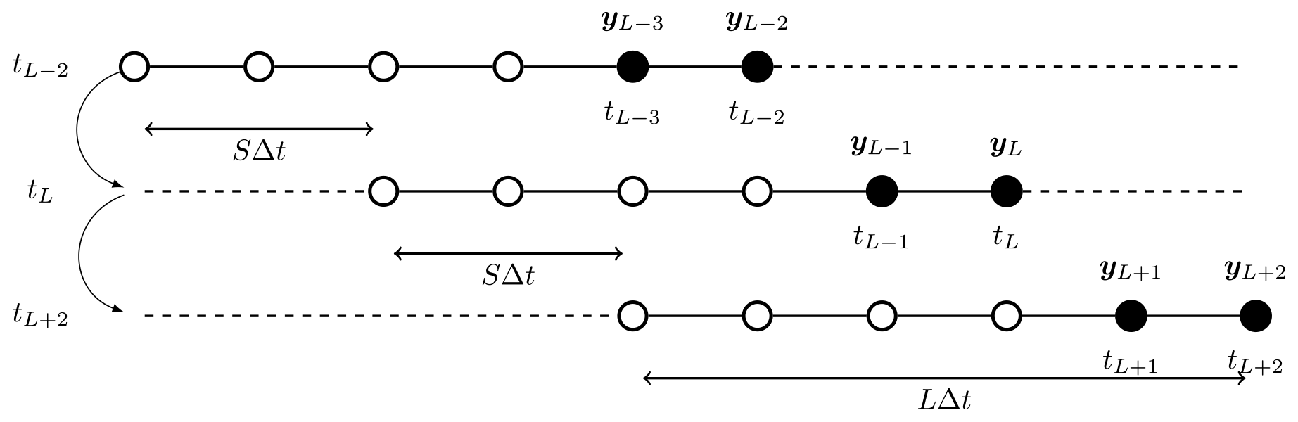
Figure 1 Three cycles of a smoother with a shift S=2 and a lag L=5. The cycle number increases from top to bottom. Time indices in the left-hand margin indicate the current time for the associated cycle of the algorithm. New observations entering the current DAW are shaded black. The initial DAW ranges from $\mathit{\{}{t}_{L-\mathrm{6}},\mathrm{\cdots },t_{L-\mathrm{2}}\mathit{\}}$. In the next cycle, this is shifted to $\mathit{\{}{t}_{L-\mathrm{4}},\mathrm{\cdots },t_L\mathit{\}}$ and is shifted thereafter to $\mathit{\{}{t}_{L-\mathrm{2}},\mathrm{\cdots },t_{L+\mathrm{2}}\mathit{\}}$. States at the zero-time indices are t_L−7 in the first cycle, t_L−5 in the second cycle, and t_L−3 in the third cycle. These are estimated in addition to states in the DAW to connect the cycles in the sequential DAWs.

Define the background mean and covariance as follows:

$$\begin{array}{}\text{(18a)}& {\displaystyle }{\stackrel{\mathrm{‾}}{\mathit{x}}}_k^i& {\displaystyle }:=\mathbb{E}\left\{{\mathit{x}}_k^i\right\},\text{(18b)}& {\displaystyle }{\mathbf{B}}_k^i& {\displaystyle }:=\mathbb{E}\left\{\left[{\mathit{x}}_k^i-{\stackrel{\mathrm{‾}}{\mathit{x}}}_k^i\right]{\left[{\mathit{x}}_k^i-{\stackrel{\mathrm{‾}}{\mathit{x}}}_k^i\right]}^{\top }\right\},\end{array}$$

where the label i refers to the density with respect to which the expectation is taken. The ensemble matrix ${\mathbf{E}}_k^i\in {\mathbb{R}}^{N_x\times N_{\mathrm{e}}}$ is likewise given a label i, denoting the conditional density according to which the ensemble is approximately distributed. The ensemble ${\mathbf{E}}_k^{\mathrm{fore}}$ is assumed to have columns sampled that are independent and identically distributed (iid), according to the forecast density. The ensemble ${\mathbf{E}}_k^{\mathrm{filt}}$ is assumed to have columns iid, according to the filter density. The ensemble ${\mathbf{E}}_{k\mathrm{|}L}^{\mathrm{smth}}$ is assumed to have columns iid according to a smoother density for the state at time t_k, given observations up to time t_L. Multiple data assimilation schemes will also utilize a balancing ensemble ${\mathbf{E}}_k^{\mathrm{bal}}$ and an MDA ensemble ${\mathbf{E}}_k^{\mathrm{mda}}$, which will be defined in Sect. 4.3. Time indices and labels may be suppressed when the meaning is still clear in the context. Note that, in realistic geophysical DA, the iid assumption rarely holds in practice, and even in the perfect linear Gaussian model, the above identifications are approximations due to the sampling error in estimating the background mean and covariance.

The forecast model is given by ${\mathbf{E}}_{k+\mathrm{1}}^i={\mathcal{M}}_{k+\mathrm{1}}\left({\mathbf{E}}_k^j\right)$, referring to the action of the map being applied column-wise, and where the type of ensemble input and output $i,j\in \mathit{\{}\mathrm{fore},\mathrm{filt},\mathrm{smth},\mathrm{bal},\mathrm{mda}\mathit{\}}$ (forecast/filter/smoother/balancing/MDA) is specified according to the estimation scheme. Define the composition of the forecast model as ${\mathbf{E}}_l^i={\mathcal{M}}_l\circ \mathrm{\cdots }\circ {\mathcal{M}}_k={\mathcal{M}}_{l:k}\left({\mathbf{E}}_{k-\mathrm{1}}^j\right)$. Let 1 denote the vector with all entries equal to one, such that the ensemble-based empirical mean, the ensemble perturbation matrix, and the ensemble-based empirical covariance are each defined by linear operations with conformal dimensions as follows:

$$\begin{array}{ll}\text{(19a)}& {\displaystyle }{\widehat{\mathit{x}}}_k^i& {\displaystyle }:={\mathbf{E}}_k^i\mathbf{1}/N_{\mathrm{e}},{\displaystyle }{\mathbf{X}}_k^i& {\displaystyle }:={\mathbf{E}}_k^i-{\widehat{\mathit{x}}}_k^i{\mathbf{1}}^{\top }\\ \text{(19b)}& {\displaystyle }& {\displaystyle }={\mathbf{E}}_k^i\left({\mathbf{I}}_{N_{\mathrm{e}}}-{\mathbf{11}}^{\top }/N_{\mathrm{e}}\right),\text{(19c)}& {\displaystyle }{\mathbf{P}}_k^i& {\displaystyle }:={\mathbf{X}}_k^i{\left({\mathbf{X}}_k^i\right)}^{\top }/\left(N_{\mathrm{e}}-\mathrm{1}\right),\end{array}$$

which is distinguished from the background mean ${\stackrel{\mathrm{‾}}{\mathit{x}}}_i^i$ and background covariance ${\mathbf{B}}_k^i$.

3 Deriving the SIEnKS

The ETKF analysis (Hunt et al., 2007) is utilized in the following for its popularity and efficiency and in order to emphasize the commonality and differences between other well-known smoothing schemes. However, the single-iteration framework is not restricted to any particular filter analysis, and other types of filter analysis, such as the deterministic EnKF (DEnKF) of Sakov and Oke (2008a), are compatible with the formalism and may be considered in future studies.

3.1 The ETKF

The filter problem is expressed recursively in the Bayesian MAP formalism with an algorithmically stationary DAW as follows. Suppose that there is a known filter density p(x₀|y₀) from a previous DA cycle. Using the Markov hypothesis and the independence of observation errors, we write the filter density up to proportionality, via Bayes' law, as follows:

$$\begin{array}{}\text{(20a)}& {\displaystyle }p\left({\mathit{x}}_{\mathrm{1}}\mathrm{|}{\mathit{y}}_{\mathrm{1}:\mathrm{0}}\right)& {\displaystyle }\propto p({\mathit{y}}_{\mathrm{1}}\mathrm{|}{\mathit{x}}_{\mathrm{1}},{\mathit{y}}_{\mathrm{0}})p({\mathit{x}}_{\mathrm{1}},{\mathit{y}}_{\mathrm{0}})\text{(20b)}& {\displaystyle }& {\displaystyle }\propto \underset{\left(i\right)}{\underbrace{p\left({\mathit{y}}_{\mathrm{1}}\mathrm{|}{\mathit{x}}_{\mathrm{1}}\right)}}\underset{\left(ii\right)}{\underbrace{\int p\left({\mathit{x}}_{\mathrm{1}}\mathrm{|}{\mathit{x}}_{\mathrm{0}}\right)p\left({\mathit{x}}_{\mathrm{0}}\mathrm{|}{\mathit{y}}_{\mathrm{0}}\right)\mathrm{d}{\mathit{x}}_{\mathrm{0}}}},\end{array}$$

which is the product of the (i) likelihood of the observation, given the forecast, and (ii) the forecast prior. The forecast prior (ii) is generated by the model propagation of the last filter density p(x₀|y₀), with the transition density p(x₁|x₀), marginalizing out x₀. Given a first prior, the above recursion inductively defines the forecast and filter densities, up to proportionality, at all times.

In the perfect linear Gaussian model, the forecast prior and filter densities,

$$\begin{array}{}\text{(21)}& {\displaystyle }\int p\left({\mathit{x}}_{\mathrm{1}}\mathrm{|}{\mathit{x}}_{\mathrm{0}}\right)p\left({\mathit{x}}_{\mathrm{0}}\mathrm{|}{\mathit{y}}_{\mathrm{0}}\right)\mathrm{d}{\mathit{x}}_{\mathrm{0}}\text{and}p\left({\mathit{x}}_{\mathrm{1}}\mathrm{|}{\mathit{y}}_{\mathrm{1}}\right),\end{array}$$

are Gaussian. The Kalman filter equations recursively compute the mean ${\stackrel{\mathrm{‾}}{\mathit{x}}}_{\mathrm{1}}^{\mathrm{fore}}/{\stackrel{\mathrm{‾}}{\mathit{x}}}_{\mathrm{1}}^{\mathrm{filt}}$ and covariance ${\mathbf{B}}_{\mathrm{1}}^{\mathrm{fore}}/{\mathbf{B}}_{\mathrm{1}}^{\mathrm{filt}}$ of the random model state x₁, parameterizing its distribution (Jazwinski, 1970). In this case, the filter problem can also be written in terms of the Bayesian MAP cost function, as follows:

$$\begin{array}{}\text{(22)}& {\displaystyle }\mathcal{J}\left({\mathit{x}}_{\mathrm{1}}\right){\displaystyle }={\displaystyle \frac{\mathrm{1}}{\mathrm{2}}}\parallel {\mathit{x}}_{\mathrm{1}}-{\stackrel{\mathrm{‾}}{\mathit{x}}}_{\mathrm{1}}^{\mathrm{fore}}{\parallel }_{{\mathbf{B}}_{\mathrm{1}}^{\mathrm{fore}}}^{\mathrm{2}}+{\displaystyle \frac{\mathrm{1}}{\mathrm{2}}}\parallel {\mathit{y}}_{\mathrm{1}}-{\mathbf{H}}_{\mathrm{1}}{\mathit{x}}_{\mathrm{1}}{\parallel }_{{\mathbf{R}}_{\mathrm{1}}}^{\mathrm{2}}.\end{array}$$

To render the above cost function into the right-transform analysis, define the matrix factor as follows:

$$\begin{array}{}\text{(23)}& {\displaystyle }{\mathbf{B}}_{\mathrm{1}}^{\mathrm{fore}}:={\mathbf{\Sigma }}_{\mathrm{1}}^{\mathrm{fore}}{\left({\mathbf{\Sigma }}_{\mathrm{1}}^{\mathrm{fore}}\right)}^{\top },\end{array}$$

where the choice of ${\mathbf{\Sigma }}_{\mathrm{1}}^{\mathrm{fore}}$ can be arbitrary but is typically given in terms of a singular value decomposition (SVD; Sakov and Oke, 2008b). Instead of optimizing the cost function in Eq. (22) over the state vector x₁, the optimization is equivalently written in terms of weights w, where, in the following:

$$\begin{array}{}\text{(24)}& {\displaystyle }{\mathit{x}}_{\mathrm{1}}:={\stackrel{\mathrm{‾}}{\mathit{x}}}_{\mathrm{1}}^{\mathrm{fore}}+{\mathbf{\Sigma }}_{\mathrm{1}}^{\mathrm{fore}}\mathit{w}.\end{array}$$

Thus, by rewriting Eq. (22) in terms of the weight vector w, we obtain the following:

$$\begin{array}{}\text{(25)}& {\displaystyle }\begin{array}{rl}\mathcal{J}\left(\mathit{w}\right)=& {\displaystyle \frac{\mathrm{1}}{\mathrm{2}}}\parallel \mathit{w}{\parallel }^{\mathrm{2}}+\\ & {\displaystyle \frac{\mathrm{1}}{\mathrm{2}}}\parallel {\mathit{y}}_{\mathrm{1}}-{\mathbf{H}}_{\mathrm{1}}{\stackrel{\mathrm{‾}}{\mathit{x}}}_{\mathrm{1}}^{\mathrm{fore}}-{\mathbf{H}}_{\mathrm{1}}{\mathbf{\Sigma }}_{\mathrm{1}}^{\mathrm{fore}}\mathit{w}{\parallel }_{{\mathbf{R}}_{\mathrm{1}}}^{\mathrm{2}}.\end{array}\end{array}$$

Furthermore, for the sake of compactness, we define the following notations:

$$\begin{array}{}\text{(26a)}& {\displaystyle }{\stackrel{\mathrm{‾}}{\mathit{y}}}_{\mathrm{1}}& {\displaystyle }:={\mathbf{H}}_{\mathrm{1}}{\stackrel{\mathrm{‾}}{\mathit{x}}}_{\mathrm{1}}^{\mathrm{fore}},\text{(26b)}& {\displaystyle }{\stackrel{\mathrm{‾}}{\mathit{\delta }}}_{\mathrm{1}}& {\displaystyle }:={\mathbf{R}}_{\mathrm{1}}^{-\frac{\mathrm{1}}{\mathrm{2}}}\left({\mathit{y}}_{\mathrm{1}}-{\stackrel{\mathrm{‾}}{\mathit{y}}}_{\mathrm{1}}\right),\text{(26c)}& {\displaystyle }{\mathbf{\Gamma }}_{\mathrm{1}}& {\displaystyle }:={\mathbf{R}}_{\mathrm{1}}^{-\frac{\mathrm{1}}{\mathrm{2}}}{\mathbf{H}}_{\mathrm{1}}{\mathbf{\Sigma }}_{\mathrm{1}}^{\mathrm{fore}}.\end{array}$$

The vector ${\stackrel{\mathrm{‾}}{\mathit{\delta }}}_{\mathrm{1}}$ is the innovation vector, weighted inverse proportionally to the observation uncertainty. The matrix Γ₁, in one dimension with H₁:=1, is equal to the standard deviation of the model forecast relative to the standard deviation of the observation error.

The cost function Eq. (25) is hence further reduced to the following:

$$\begin{array}{}\text{(27)}& {\displaystyle }\mathcal{J}\left(\mathit{w}\right)={\displaystyle \frac{\mathrm{1}}{\mathrm{2}}}\parallel \mathit{w}{\parallel }^{\mathrm{2}}+{\displaystyle \frac{\mathrm{1}}{\mathrm{2}}}\parallel {\stackrel{\mathrm{‾}}{\mathit{\delta }}}_{\mathrm{1}}-{\mathbf{\Gamma }}_{\mathrm{1}}\mathit{w}{\parallel }^{\mathrm{2}}.\end{array}$$

This cost function is quadratic in w and can be globally minimized where ∇_w𝒥=0. Notice that, in the following:

$$\begin{array}{}\text{(28)}& {\displaystyle }{\mathrm{\nabla }}_{\mathit{w}}\mathcal{J}=\mathit{w}-{\mathbf{\Gamma }}_{\mathrm{1}}^{\top }\left({\stackrel{\mathrm{‾}}{\mathit{\delta }}}_{\mathrm{1}}-{\mathbf{\Gamma }}_{\mathrm{1}}\mathit{w}\right).\end{array}$$

By setting the gradient equal to zero for $\stackrel{\mathrm{‾}}{\mathit{w}}$, we find the following expression for the optimal weights:

$$\begin{array}{}\text{(29a)}& {\displaystyle }& {\displaystyle }\mathbf{0}=\stackrel{\mathrm{‾}}{\mathit{w}}-{\mathbf{\Gamma }}_{\mathrm{1}}^{\top }\left({\stackrel{\mathrm{‾}}{\mathit{\delta }}}_{\mathrm{1}}-{\mathbf{\Gamma }}_{\mathrm{1}}\stackrel{\mathrm{‾}}{\mathit{w}}\right)\text{(29b)}& {\displaystyle }\iff & {\displaystyle }{\mathbf{\Gamma }}_{\mathrm{1}}^{\top }{\stackrel{\mathrm{‾}}{\mathit{\delta }}}_{\mathrm{1}}=\left({\mathbf{I}}_{N_x}+{\mathbf{\Gamma }}_{\mathrm{1}}^{\top }{\mathbf{\Gamma }}_{\mathrm{1}}\right)\stackrel{\mathrm{‾}}{\mathit{w}}\text{(29c)}& {\displaystyle }\iff & {\displaystyle }\stackrel{\mathrm{‾}}{\mathit{w}}={\left({\mathbf{I}}_{N_x}+{\mathbf{\Gamma }}_{\mathrm{1}}^{\top }{\mathbf{\Gamma }}_{\mathrm{1}}\right)}^{-\mathrm{1}}{\mathbf{\Gamma }}_{\mathrm{1}}^{\top }{\stackrel{\mathrm{‾}}{\mathit{\delta }}}_{\mathrm{1}}.\end{array}$$

From Eq. (28), notice that

$$\begin{array}{}\text{(30)}& {\displaystyle }{\mathrm{\nabla }}_{\mathit{w}}\mathcal{J}{\mathrm{|}}_{\mathit{w}=\mathbf{0}}=-{\mathbf{\Gamma }}_{\mathrm{1}}^{\top }{\stackrel{\mathrm{‾}}{\mathit{\delta }}}_{\mathrm{1}}.\end{array}$$

Similarly, taking the gradient of Eq. (28), we find that the Hessian, ${\mathbf{\Xi }}_{\mathcal{J}}:={\mathrm{\nabla }}_{\mathit{w}}^{\mathrm{2}}\mathcal{J}$, is equal to the following:

$$\begin{array}{}\text{(31)}& {\displaystyle }{\mathbf{\Xi }}_{\mathcal{J}}=\left({\mathbf{I}}_{N_x}+{\mathbf{\Gamma }}_{\mathrm{1}}^{\top }{\mathbf{\Gamma }}_{\mathrm{1}}\right).\end{array}$$

Therefore, with w=0 corresponding to ${\stackrel{\mathrm{‾}}{\mathit{x}}}_{\mathrm{1}}^{\mathrm{fore}}$ as the initialization of the algorithm, the MAP weights $\stackrel{\mathrm{‾}}{\mathit{w}}$ are determined by a single iteration of Newton's descent method (Nocedal and Wright, 2006). For iterate i, this has the general form of the following:

$$\begin{array}{}\text{(32)}& {\displaystyle }{\mathit{w}}^{i+\mathrm{1}}:={\mathit{w}}^i-{\mathbf{\Xi }}_{\mathcal{J}}^{-\mathrm{1}}\mathrm{\nabla }\mathcal{J}{\mathrm{|}}_{\mathit{w}={\mathit{w}}^i}.\end{array}$$

The MAP weights define the maximum a posteriori model state as follows:

$$\begin{array}{}\text{(33)}& {\displaystyle }{\stackrel{\mathrm{‾}}{\mathit{x}}}_{\mathrm{1}}^{\mathrm{filt}}:={\stackrel{\mathrm{‾}}{\mathit{x}}}_{\mathrm{1}}^{\mathrm{fore}}+{\mathbf{\Sigma }}_{\mathrm{1}}^{\mathrm{fore}}\stackrel{\mathrm{‾}}{\mathit{w}}.\end{array}$$

Under the perfect linear Gaussian model assumption, 𝒥 can then be rewritten in terms of the filter MAP estimate as follows:

$$\begin{array}{}\text{(34a)}& {\displaystyle }& {\displaystyle }\mathcal{J}\left({\mathit{x}}_{\mathrm{1}}\right)={\displaystyle \frac{\mathrm{1}}{\mathrm{2}}}\parallel {\mathit{x}}_{\mathrm{1}}-{\stackrel{\mathrm{‾}}{\mathit{x}}}_{\mathrm{1}}^{\mathrm{filt}}{\parallel }_{{\mathbf{B}}_{\mathrm{1}}^{\mathrm{filt}}}^{\mathrm{2}}\text{(34b)}& {\displaystyle }\iff & {\displaystyle }\mathcal{J}\left(\mathit{w}\right)={\displaystyle \frac{\mathrm{1}}{\mathrm{2}}}\parallel {\stackrel{\mathrm{‾}}{\mathit{x}}}_{\mathrm{1}}^{\mathrm{fore}}-{\mathbf{\Sigma }}_{\mathrm{1}}^{\mathrm{fore}}\mathit{w}-{\stackrel{\mathrm{‾}}{\mathit{x}}}_{\mathrm{1}}^{\mathrm{filt}}{\parallel }_{{\mathbf{B}}_{\mathrm{1}}^{\mathrm{filt}}}^{\mathrm{2}}.\end{array}$$

Define the matrix decomposition ${\mathbf{B}}_{\mathrm{1}}^{\mathrm{filt}}={\mathbf{\Sigma }}_{\mathrm{1}}^{\mathrm{filt}}{\left({\mathbf{\Sigma }}_{\mathrm{1}}^{\mathrm{filt}}\right)}^{\top }$ and the change in variables as follows:

$$\begin{array}{}\text{(35a)}& {\displaystyle }{\mathbf{\Omega }}_{\mathrm{1}}& {\displaystyle }:={\left({\mathbf{\Sigma }}_{\mathrm{1}}^{\mathrm{filt}}\right)}^{-\mathrm{1}}{\mathbf{\Sigma }}_{\mathrm{1}}^{\mathrm{fore}},\text{(35b)}& {\displaystyle }{\mathit{\varrho }}_{\mathrm{1}}& {\displaystyle }:={\left({\mathbf{\Sigma }}_{\mathrm{1}}^{\mathrm{filt}}\right)}^{-\mathrm{1}}\left({\stackrel{\mathrm{‾}}{\mathit{x}}}_{\mathrm{1}}^{\mathrm{fore}}-{\stackrel{\mathrm{‾}}{\mathit{x}}}_{\mathrm{1}}^{\mathrm{filt}}\right).\end{array}$$

Then, Eq. (34b) can be rewritten as follows:

$$\begin{array}{}\text{(36)}& {\displaystyle }\mathcal{J}\left(\mathit{w}\right)={\displaystyle \frac{\mathrm{1}}{\mathrm{2}}}\parallel {\mathit{\varrho }}_{\mathrm{1}}-{\mathbf{\Omega }}_{\mathrm{1}}\mathit{w}{\parallel }^{\mathrm{2}}.\end{array}$$

Computing the Hessian ${\mathbf{\Xi }}_{\mathcal{J}}={\mathrm{\nabla }}_{\mathit{w}}^{\mathrm{2}}\mathcal{J}$ from each of Eqs. (27) and (36), we find, by their equivalence, the following:

$$\begin{array}{}\text{(37a)}& {\displaystyle }& {\displaystyle }\left({\mathbf{I}}_{N_x}+{\mathbf{\Gamma }}_{\mathrm{1}}^{\top }{\mathbf{\Gamma }}_{\mathrm{1}}\right)={\mathbf{\Omega }}_{\mathrm{1}}^{\top }{\mathbf{\Omega }}_{\mathrm{1}}\text{(37b)}& {\displaystyle }\iff & {\displaystyle }\left({\mathbf{I}}_{N_x}+{\mathbf{\Gamma }}_{\mathrm{1}}^{\top }{\mathbf{\Gamma }}_{\mathrm{1}}\right)={\left({\mathbf{\Sigma }}_{\mathrm{1}}^{\mathrm{fore}}\right)}^{\top }{\left({\mathbf{\Sigma }}_{\mathrm{1}}^{\mathrm{filt}}\right)}^{-\top }{\left({\mathbf{\Sigma }}_{\mathrm{1}}^{\mathrm{filt}}\right)}^{-\mathrm{1}}{\mathbf{\Sigma }}_{\mathrm{1}}^{\mathrm{fore}}\text{(37c)}& {\displaystyle }\iff & {\displaystyle }{\mathbf{B}}_{\mathrm{1}}^{\mathrm{filt}}={\mathbf{\Sigma }}_{\mathrm{1}}^{\mathrm{fore}}{\left({\mathbf{I}}_{N_x}+{\mathbf{\Gamma }}_{\mathrm{1}}^{\top }{\mathbf{\Gamma }}_{\mathrm{1}}\right)}^{-\mathrm{1}}{\left({\mathbf{\Sigma }}_{\mathrm{1}}^{\mathrm{fore}}\right)}^{\top }.\end{array}$$

If we define the covariance transform as

$$\begin{array}{}\text{(38)}& {\displaystyle }\mathbf{T}:={\mathbf{\Xi }}_{\mathcal{J}}^{-\frac{\mathrm{1}}{\mathrm{2}}},\end{array}$$

then this derivation above describes the square root Kalman filter recursion (Tippett et al., 2003) when written for the exact mean and covariance, which is recursively computed in the perfect linear Gaussian model. The covariance update is then as follows:

$$\begin{array}{}\text{(39)}& {\displaystyle }{\mathbf{B}}_{\mathrm{1}}^{\mathrm{filt}}=\left({\mathbf{\Sigma }}_{\mathrm{1}}^{\mathrm{fore}}\mathbf{T}\right){\left({\mathbf{\Sigma }}_{\mathrm{1}}^{\mathrm{fore}}\mathbf{T}\right)}^{\top }.\end{array}$$

It is written entirely in terms of the matrix factor ${\mathbf{\Sigma }}_k^i$ and the covariance transform T, such that the background covariance need not be explicitly computed in order to produce recursive estimates. Likewise, the Kalman gain update to the mean state is reduced to Eq. (33) in terms of the weights and the matrix factor. This reduction is at the core of the efficiency of the ETKF in which one typically makes a reduced-rank approximation to the background covariances ${\mathbf{B}}_{\mathrm{1}}^i$.

Using the ensemble-based empirical estimates for the background, as in Eq. (19), a modification of the above argument must be used to solve the cost function 𝒥 in the ensemble span, without a direct inversion of ${\mathbf{P}}_{\mathrm{1}}^{\mathrm{fore}}$ when this is of a reduced rank. We replace the background covariance norm square with one defined by the ensemble-based covariance, as follows:

$$\begin{array}{}\text{(40)}& {\displaystyle }\parallel \mathit{v}{\parallel }_{{\mathbf{P}}_{\mathrm{1}}^i}^{\mathrm{2}}{\displaystyle }=\left(N_{\mathrm{e}}-\mathrm{1}\right){\left[{\left({\mathbf{X}}_{\mathrm{1}}^i\right)}^{†}\mathit{v}\right]}^{\top }\left[{\left({\mathbf{X}}_{\mathrm{1}}^i\right)}^{†}\mathit{v}\right].\end{array}$$

We then define the ensemble-based estimates as follows:

$$\begin{array}{}\text{(41a)}& {\displaystyle }{\mathit{x}}_{\mathrm{1}}& {\displaystyle }:={\widehat{\mathit{x}}}_{\mathrm{1}}^{\mathrm{fore}}+{\mathbf{X}}_{\mathrm{1}}^{\mathrm{fore}}\mathit{w},\text{(41b)}& {\displaystyle }{\widehat{\mathit{y}}}_{\mathrm{1}}& {\displaystyle }:={\mathbf{H}}_{\mathrm{1}}{\widehat{\mathit{x}}}_{\mathrm{1}}^{\mathrm{fore}},\text{(41c)}& {\displaystyle }{\widehat{\mathit{\delta }}}_{\mathrm{1}}& {\displaystyle }:={\mathbf{R}}_{\mathrm{1}}^{-\frac{\mathrm{1}}{\mathrm{2}}}\left({\mathit{y}}_{\mathrm{1}}-{\widehat{\mathit{y}}}_{\mathrm{1}}\right),\text{(41d)}& {\displaystyle }{\mathbf{S}}_{\mathrm{1}}& {\displaystyle }:={\mathbf{R}}_{\mathrm{1}}^{-\frac{\mathrm{1}}{\mathrm{2}}}{\mathbf{H}}_{\mathrm{1}}{\mathbf{X}}_{\mathrm{1}}^{\mathrm{fore}},\end{array}$$

where w is now a weight vector in ${\mathbb{R}}^{N_{\mathrm{e}}}$. The ensemble-based cost function is then written as follows:

$$\begin{array}{ll}{\displaystyle }\stackrel{\mathrm{̃}}{\mathcal{J}}\left(\mathit{w}\right)=& {\displaystyle \frac{\mathrm{1}}{\mathrm{2}}}\parallel {\widehat{\mathit{x}}}_{\mathrm{1}}^{\mathrm{fore}}-{\mathbf{X}}_{\mathrm{1}}^{\mathrm{fore}}\mathit{w}-{\widehat{\mathit{x}}}_{\mathrm{1}}^{\mathrm{fore}}{\parallel }_{{\mathbf{P}}_{\mathrm{1}}^{\mathrm{fore}}}^{\mathrm{2}}+\\ \text{(42a)}& {\displaystyle }& {\displaystyle \frac{\mathrm{1}}{\mathrm{2}}}\parallel {\mathit{y}}_{\mathrm{1}}-{\mathbf{H}}_{\mathrm{1}}{\widehat{\mathit{x}}}_{\mathrm{1}}^{\mathrm{fore}}-{\mathbf{H}}_{\mathrm{1}}{\mathbf{X}}_{\mathrm{1}}^{\mathrm{fore}}\mathit{w}{\parallel }_{{\mathbf{R}}_{\mathrm{1}}}^{\mathrm{2}}\text{(42b)}& {\displaystyle }=& {\displaystyle \frac{\mathrm{1}}{\mathrm{2}}}(N_{\mathrm{e}}-\mathrm{1})\parallel \mathit{w}{\parallel }^{\mathrm{2}}+{\displaystyle \frac{\mathrm{1}}{\mathrm{2}}}\parallel {\widehat{\mathit{\delta }}}_{\mathrm{1}}-{\mathbf{S}}_{\mathrm{1}}\mathit{w}{\parallel }^{\mathrm{2}}.\end{array}$$

Define $\widehat{\mathit{w}}$ to be the minimizer of the cost function in Eq. (42). Hunt et al. (2007) demonstrate that, up to a gauge transformation, $\widehat{\mathit{w}}$ yields the minimizer of the state space cost function, Eq. (22), when the estimate is restricted to the ensemble span. Let ${\stackrel{\mathrm{̃}}{\mathbf{\Xi }}}_{\stackrel{\mathrm{̃}}{\mathcal{J}}}$ denote the Hessian of the ensemble-based cost function in Eq. (42). This equation is quadratic in w and can be solved similarly to Eq. (27) to render the following:

$$\begin{array}{}\text{(43a)}& {\displaystyle }\widehat{\mathit{w}}:=& {\displaystyle }\mathbf{0}-{\stackrel{\mathrm{̃}}{\mathbf{\Xi }}}_{\stackrel{\mathrm{̃}}{\mathcal{J}}}^{-\mathrm{1}}\mathrm{\nabla }\stackrel{\mathrm{̃}}{\mathcal{J}}{|}_{\mathit{w}=\mathbf{0}},\text{(43b)}& {\displaystyle }\mathbf{T}:=& {\displaystyle }{\stackrel{\mathrm{̃}}{\mathbf{\Xi }}}_{\stackrel{\mathrm{̃}}{\mathcal{J}}}^{-\frac{\mathrm{1}}{\mathrm{2}}},\text{(43c)}& {\displaystyle }{\mathbf{P}}_{\mathrm{1}}^{\mathrm{filt}}=& {\displaystyle }\left({\mathbf{X}}_{\mathrm{1}}^{\mathrm{fore}}\mathbf{T}\right){\left({\mathbf{X}}_{\mathrm{1}}^{\mathrm{fore}}\mathbf{T}\right)}^{\top }/(N_{\mathrm{e}}-\mathrm{1}).\end{array}$$

The ensemble transform Kalman filter (ETKF) equations are then given by the following:

$$\begin{array}{}\text{(44)}& {\displaystyle }{\mathbf{E}}_{\mathrm{1}}^{\mathrm{filt}}={\widehat{\mathit{x}}}_{\mathrm{1}}^{\mathrm{fore}}{\mathbf{1}}^{\top }+{\mathbf{X}}_{\mathrm{1}}^{\mathrm{fore}}\left(\widehat{\mathit{w}}{\mathbf{1}}^{\top }+\sqrt{N_{\mathrm{e}}-\mathrm{1}}\mathbf{TU}\right),\end{array}$$

where $\mathbf{U}\in {\mathbb{R}}^{N_{\mathrm{e}}\times N_{\mathrm{e}}}$ can be any mean-preserving, orthogonal transformation, i.e., U1=1. The simple choice of $\mathbf{U}:={\mathbf{I}}_{N_{\mathrm{e}}}$ is sufficient, but it has been demonstrated that choosing a random, mean-preserving orthogonal transformation at each analysis, as above, can improve the stability of the ETKF, preventing the collapse of the variances to a few modes in the empirical covariance estimate (Sakov and Oke, 2008b). We remark that Eq. (44) can be written equivalently as a single linear transformation as follows:

$$\begin{array}{ll}\text{(45a)}& {\displaystyle }{\mathbf{E}}_{\mathrm{1}}^{\mathrm{filt}}=& {\displaystyle }{\mathbf{E}}_{\mathrm{1}}^{\mathrm{fore}}{\mathbf{\Psi }}_{\mathrm{1}},{\displaystyle }{\mathbf{\Psi }}_{\mathrm{1}}:=& {\displaystyle }{\mathbf{11}}^{\top }/N_{\mathrm{e}}+\\ \text{(45b)}& {\displaystyle }& {\displaystyle }\left({\mathbf{I}}_{N_{\mathrm{e}}}-{\mathbf{11}}^{\top }/N_{\mathrm{e}}\right)\left(\widehat{\mathit{w}}{\mathbf{1}}^{\top }+\sqrt{N_{\mathrm{e}}-\mathrm{1}}\mathbf{TU}\right).\end{array}$$

The compact update notation in Eq. (45) is used to simplify the analysis.

If the observation operator ℋ₁ is actually nonlinear, then the ETKF typically uses the following approximation to the quadratic cost function:

$$\begin{array}{}\text{(46a)}& {\displaystyle }{\mathbf{Y}}_{\mathrm{1}}& {\displaystyle }:={\mathcal{H}}_{\mathrm{1}}\left({\mathbf{E}}_{\mathrm{1}}^{\mathrm{fore}}\right),\text{(46b)}& {\displaystyle }{\widehat{\mathit{y}}}_{\mathrm{1}}& {\displaystyle }:={\mathbf{Y}}_{\mathrm{1}}\mathbf{1}/N_{\mathrm{e}},\text{(46c)}& {\displaystyle }{\mathbf{S}}_{\mathrm{1}}& {\displaystyle }:={\mathbf{R}}_{\mathrm{1}}^{-\frac{\mathrm{1}}{\mathrm{2}}}{\mathbf{Y}}_{\mathrm{1}}-{\widehat{\mathit{y}}}_{\mathrm{1}}{\mathbf{1}}^{\top },\end{array}$$

where term (46a) refers to the action of the observation operator being applied column-wise. Substituting the definitions in Eq. (46) for the definitions in Eq. (41) gives the standard nonlinear analysis in the ETKF. Note that this framework extends to a fully iterative analysis of nonlinear observation operators, as discussed in Sect. 4.1. Multiplicative covariance inflation is often used in the ETKF to handle the systematic underestimation of the forecast and filter covariance due to the sample error implied by a finite size ensemble and nonlinearity of the forecast model ℳ₁ (Raanes et al., 2019a).

The standard ETKF cycle is summarized in Algorithm A5. This algorithm is broken into the subroutines, in Algorithms A1–A4, which are reused throughout our analysis to emphasize the commonality and the differences in the studied smoother schemes. The filter analysis described above can be extended in several different ways when producing a smoother analysis on a DAW, including lagged past states, depending in part on whether it is formulated as a marginal or a joint smoother (Cosme et al., 2012). The way in which this analysis is extended, utilizing a retrospective reanalysis or a 4D cost function, differentiates the EnKS from the IEnKS and highlights the ways in which the SIEnKS differs from these other schemes.

3.2 The fixed-lag EnKS

The (right-transform) fixed-lag EnKS extends the ETKF over the smoothing DAW by sequentially reanalyzing past states with future observations. This analysis is performed retrospectively in the sense that the filter cycle of the ETKF is left unchanged, while an additional smoother loop of the DA cycle performs an update on the lagged state ensembles stored in memory. Assume $S=\mathrm{1}\le L$, then the EnKS estimates the joint posterior density $p\left({\mathit{x}}_{L:\mathrm{1}}\mathrm{|}{\mathit{y}}_{L:\mathrm{1}}\right)$ recursively, given the joint posterior estimate over the last DAW $p\left({\mathit{x}}_{L-\mathrm{1}:\mathrm{0}}\mathrm{|}{\mathit{y}}_{L-\mathrm{1}:\mathrm{0}}\right)$. We begin by considering the filter problem as in Eq. (20).

Given $p({\mathit{x}}_{L-\mathrm{1}:\mathrm{0}},{\mathit{y}}_{L-\mathrm{1}:\mathrm{0}})$, we write the filter density up to proportionality as follows:

$$\begin{array}{ll}\text{(47a)}& {\displaystyle }p\left({\mathit{x}}_L\mathrm{|}{\mathit{y}}_{L:\mathrm{0}}\right)\propto & {\displaystyle }p({\mathit{y}}_L\mathrm{|}{\mathit{x}}_L,{\mathit{y}}_{L-\mathrm{1}:\mathrm{0}})p({\mathit{x}}_L,{\mathit{y}}_{L-\mathrm{1}:\mathrm{0}}){\displaystyle }\propto & {\displaystyle }\underset{\left(\mathrm{i}\right)}{\underbrace{p\left({\mathit{y}}_L\mathrm{|}{\mathit{x}}_L\right)}}\times \\ \text{(47b)}& {\displaystyle }& {\displaystyle }\underset{\left(\mathrm{ii}\right)}{\underbrace{\int p\left({\mathit{x}}_L\mathrm{|}{\mathit{x}}_{L-\mathrm{1}}\right)p\left({\mathit{x}}_{L-\mathrm{1}:\mathrm{0}}\mathrm{|}{\mathit{y}}_{L-\mathrm{1}:\mathrm{0}}\right)\mathrm{d}{\mathit{x}}_{L-\mathrm{1}:\mathrm{0}}}},\end{array}$$

with the product of (i) the likelihood of the observation y_L, given x_L, and (ii) the forecast for x_L, using the transition kernel on the last joint posterior estimate and marginalizing out ${\mathit{x}}_{L-\mathrm{1}:\mathrm{0}}$. Recalling that $p\left({\mathit{x}}_L\mathrm{|}{\mathit{y}}_{L:\mathrm{1}}\right)\propto p\left({\mathit{x}}_L\mathrm{|}{\mathit{y}}_{L:\mathrm{0}}\right)$, this provides a means to sample the filter marginal of the desired joint posterior. The usual ETKF filter analysis is performed to sample the filter distribution at time t_L; yet, to complete the smoothing cycle, the scheme must sample the joint posterior density $p({\mathit{x}}_{L:\mathrm{1}},{\mathit{y}}_{L:\mathrm{1}})$.

Consider that the marginal smoother density is proportional to the following:

$$\begin{array}{ll}{\displaystyle }p\left({\mathit{x}}_{L-\mathrm{1}}\mathrm{|}{\mathit{y}}_{L:\mathrm{0}}\right)\propto & {\displaystyle }p({\mathit{y}}_L\mathrm{|}{\mathit{x}}_{L-\mathrm{1}},{\mathit{y}}_{L-\mathrm{1}:\mathrm{0}})\times \\ \text{(48a)}& {\displaystyle }& {\displaystyle }p({\mathit{x}}_{L-\mathrm{1}},{\mathit{y}}_{L-\mathrm{1}:\mathrm{0}})\text{(48b)}& {\displaystyle }\propto & {\displaystyle }\underset{\left(\mathrm{i}\right)}{\underbrace{p\left({\mathit{y}}_L\mathrm{|}{\mathit{x}}_{L-\mathrm{1}}\right)}}\underset{\left(\mathrm{ii}\right)}{\underbrace{p\left({\mathit{x}}_{L-\mathrm{1}}\mathrm{|}{\mathit{y}}_{L-\mathrm{1}:\mathrm{0}}\right)}},\end{array}$$

where (i) is the likelihood of the observation y_L, given the past state x_L−1, and (ii) is the marginal density for x_L−1 from the last joint posterior.

Assume now the perfect linear Gaussian model; then, the corresponding Bayesian MAP cost function is given as follows:

$$\begin{array}{}\text{(49)}& {\displaystyle }\begin{array}{rl}\mathcal{J}\left({\mathit{x}}_{L-\mathrm{1}}\right)=& {\displaystyle \frac{\mathrm{1}}{\mathrm{2}}}\parallel {\mathit{x}}_{L-\mathrm{1}}-{\stackrel{\mathrm{‾}}{\mathit{x}}}_{L-\mathrm{1}|L-\mathrm{1}}^{\mathrm{smth}}{\parallel }_{{\mathbf{B}}_{L-\mathrm{1}|L-\mathrm{1}}^{\mathrm{smth}}}^{\mathrm{2}}+\\ & {\displaystyle \frac{\mathrm{1}}{\mathrm{2}}}\parallel {\mathit{y}}_L-{\mathbf{H}}_L{\mathbf{M}}_L{\mathit{x}}_{L-\mathrm{1}}{\parallel }_{{\mathbf{R}}_L}^{\mathrm{2}},\end{array}\end{array}$$

where ${\stackrel{\mathrm{‾}}{\mathit{x}}}_{L-\mathrm{1}|L-\mathrm{1}}^{\mathrm{smth}}$ and ${\mathbf{B}}_{L-\mathrm{1}|L-\mathrm{1}}^{\mathrm{smth}}$ are the mean and covariance of the marginal smoother density $p\left({\mathit{x}}_{L-\mathrm{1}}\mathrm{|}{\mathit{y}}_{L-\mathrm{1}:\mathrm{0}}\right)$. Take the following matrix decomposition:

$$\begin{array}{}\text{(50)}& {\displaystyle }{\mathbf{B}}_{L-\mathrm{1}|L-\mathrm{1}}^{\mathrm{smth}}={\mathbf{\Sigma }}_{L-\mathrm{1}|L-\mathrm{1}}^{\mathrm{smth}}{\left({\mathbf{\Sigma }}_{L-\mathrm{1}|L-\mathrm{1}}^{\mathrm{smth}}\right)}^{\top }.\end{array}$$

Then, write ${\mathit{x}}_{L-\mathrm{1}}={\stackrel{\mathrm{‾}}{\mathit{x}}}_{L-\mathrm{1}|L-\mathrm{1}}^{\mathrm{smth}}+{\mathbf{\Sigma }}_{L-\mathrm{1}|L-\mathrm{1}}^{\mathrm{smth}}\mathit{w}$, rendering the cost function as follows:

$$\begin{array}{ll}{\displaystyle }\mathcal{J}\left(\mathit{w}\right)=& {\displaystyle \frac{\mathrm{1}}{\mathrm{2}}}\parallel \mathit{w}{\parallel }^{\mathrm{2}}+\\ \text{(51a)}& {\displaystyle }& {\displaystyle \frac{\mathrm{1}}{\mathrm{2}}}\parallel {\mathit{y}}_L-{\mathbf{H}}_L{\mathbf{M}}_L({\stackrel{\mathrm{‾}}{\mathit{x}}}_{L-\mathrm{1}|L-\mathrm{1}}^{\mathrm{smth}}+{\mathbf{\Sigma }}_{L-\mathrm{1}|L-\mathrm{1}}^{\mathrm{smth}}\mathit{w}){\parallel }_{{\mathbf{R}}_L}^{\mathrm{2}}\text{(51b)}& {\displaystyle }=& {\displaystyle \frac{\mathrm{1}}{\mathrm{2}}}\parallel \mathit{w}{\parallel }^{\mathrm{2}}+{\displaystyle \frac{\mathrm{1}}{\mathrm{2}}}\parallel {\mathit{y}}_L-{\mathbf{H}}_L{\stackrel{\mathrm{‾}}{\mathit{x}}}_L^{\mathrm{fore}}-{\mathbf{H}}_L{\mathbf{\Sigma }}_L^{\mathrm{fore}}\mathit{w}{\parallel }_{{\mathbf{R}}_L}^{\mathrm{2}}\text{(51c)}& {\displaystyle }=& {\displaystyle \frac{\mathrm{1}}{\mathrm{2}}}\parallel \mathit{w}{\parallel }^{\mathrm{2}}+{\displaystyle \frac{\mathrm{1}}{\mathrm{2}}}\parallel {\stackrel{\mathrm{‾}}{\mathit{\delta }}}_L-{\mathbf{\Gamma }}_L\mathit{w}{\parallel }^{\mathrm{2}}.\end{array}$$

Let $\stackrel{\mathrm{‾}}{\mathit{w}}$ now denote the minimizer of Eq. (51). It is important to recognize that

$$\begin{array}{}\text{(52)}& {\displaystyle }{\mathit{x}}_L& {\displaystyle }:={\mathbf{M}}_L\left({\stackrel{\mathrm{‾}}{\mathit{x}}}_{L-\mathrm{1}|L-\mathrm{1}}^{\mathrm{smth}}+{\mathbf{\Sigma }}_{L-\mathrm{1}|L-\mathrm{1}}^{\mathrm{smth}}\mathit{w}\right)\text{(53)}& {\displaystyle }& {\displaystyle }={\stackrel{\mathrm{‾}}{\mathit{x}}}_L^{\mathrm{fore}}+{\mathbf{\Sigma }}_L^{\mathrm{fore}}\mathit{w},\end{array}$$

such that the optimal weight vector for the smoothing problem $\stackrel{\mathrm{‾}}{\mathit{w}}$ is also the optimal weight vector for the filter problem.

The ensemble-based approximation,

$$\begin{array}{}\text{(54a)}& {\displaystyle }{\mathit{x}}_{L-\mathrm{1}}& {\displaystyle }={\widehat{\mathit{x}}}_{L-\mathrm{1}|L-\mathrm{1}}^{\mathrm{smth}}+{\mathbf{X}}_{L-\mathrm{1}|L-\mathrm{1}}^{\mathrm{smth}}\mathit{w},\text{(54b)}& {\displaystyle }\stackrel{\mathrm{̃}}{\mathcal{J}}\left(\mathit{w}\right)& {\displaystyle }={\displaystyle \frac{\mathrm{1}}{\mathrm{2}}}(N_{\mathrm{e}}-\mathrm{1})\parallel \mathit{w}{\parallel }^{\mathrm{2}}+{\displaystyle \frac{\mathrm{1}}{\mathrm{2}}}\parallel {\widehat{\mathit{\delta }}}_L-{\mathbf{S}}_L\mathit{w}{\parallel }^{\mathrm{2}},\end{array}$$

to the exact smoother cost function in Eq. (51) yields the retrospective analysis of the EnKS as follows:

$$\begin{array}{ll}\text{(55a)}& {\displaystyle }\widehat{\mathit{w}}:=& {\displaystyle }\mathbf{0}-{\stackrel{\mathrm{̃}}{\mathbf{\Xi }}}_{\stackrel{\mathrm{̃}}{\mathcal{J}}}^{-\mathrm{1}}\mathrm{\nabla }\stackrel{\mathrm{̃}}{\mathcal{J}}{|}_{\mathit{w}=\mathbf{0}},\text{(55b)}& {\displaystyle }\mathbf{T}:=& {\displaystyle }{\stackrel{\mathrm{̃}}{\mathbf{\Xi }}}_{\stackrel{\mathrm{̃}}{\mathcal{J}}}^{-\frac{\mathrm{1}}{\mathrm{2}}},{\displaystyle }{\mathbf{E}}_{L-\mathrm{1}|L}^{\mathrm{smth}}=& {\displaystyle }{\widehat{\mathit{x}}}_{L-\mathrm{1}|L-\mathrm{1}}^{\mathrm{smth}}{\mathbf{1}}^{\top }+\\ \text{(55c)}& {\displaystyle }& {\displaystyle }{\mathbf{X}}_{L-\mathrm{1}|L-\mathrm{1}}^{\mathrm{smth}}\left(\widehat{\mathit{w}}{\mathbf{1}}^{\top }+\sqrt{N_{\mathrm{e}}-\mathrm{1}}\mathbf{TU}\right),\text{(55d)}& {\displaystyle }\equiv & {\displaystyle }{\mathbf{E}}_{L-\mathrm{1}|L-\mathrm{1}}^{\mathrm{smth}}{\mathbf{\Psi }}_L.\end{array}$$

The above equations generalize for arbitrary indices k|L, completely describing the smoother loop between each filter cycle of the EnKS. After a new observation is assimilated with the ETKF analysis step, a smoother loop makes a backwards pass over the DAW, applying the transform and the weights of the ETKF filter update to each past state ensemble stored in memory. This generalizes to the case where there is a shift in the DAW with S>1, though the EnKS does not process observations asynchronously by default, i.e., the ETKF filter steps, and the subsequent retrospective reanalysis, are performed in sequence over the observations and ordered in time rather than making a global analysis over ${\mathit{y}}_{L:L-S+\mathrm{1}}$. A standard form of the EnKS is summarized in Algorithm A6, utilizing the subroutines in Algorithms A1–A4.

A schematic of the EnKS cycle for a lag of L=4 and a shift of S=1 is pictured in Fig. 2. Time moves forwards, from left to right, on the horizontal axis, with a step size of Δt. At each analysis time, the ensemble forecast from the last filter density is combined with the observation to produce the ensemble update transform Ψ_L. This transform is then utilized to produce the posterior estimate for all lagged state ensembles conditioned on the new observation. The information in the posterior estimate thus flows in reverse time to the lagged states stored in memory, but the information flow is unidirectional in this scheme. It is understood then that reinitializing the improved posterior estimate for the lagged states in the dynamical model does not improve the filter estimate in the perfect linear Gaussian configuration. Indeed, define the product of the ensemble transforms as follows:

$$\begin{array}{}\text{(56)}& {\displaystyle }{\mathbf{\Psi }}_{k:l}:={\mathbf{\Psi }}_k\mathrm{\cdots }{\mathbf{\Psi }}_l.\end{array}$$

Then, for arbitrary $\mathrm{1}\le k\le l\le L$,

$$\begin{array}{}\text{(57a)}& {\displaystyle }{\mathbf{M}}_{l:k}{\mathbf{E}}_{k-\mathrm{1}|k-\mathrm{1}}^{\mathrm{smth}}{\mathbf{\Psi }}_{k:l}& {\displaystyle }={\mathbf{M}}_{l:k}{\mathbf{E}}_{k-\mathrm{1}|l}^{\mathrm{smth}}\text{(57b)}& {\displaystyle }& {\displaystyle }={\mathbf{E}}_{l|k-\mathrm{1}}^{\mathrm{fore}}{\mathbf{\Psi }}_{k:l}\text{(57c)}& {\displaystyle }& {\displaystyle }={\mathbf{E}}_{l|l}^{\mathrm{smth}}.\end{array}$$

This demonstrates that conditioning on the information from the observation is covariant with the dynamics. Raanes (2016) demonstrates the equivalence of the EnKS and the Rauch–Tung–Striebel (RTS) smoother, where this property of perfect linear Gaussian models is well understood. In the RTS formulation of the retrospective reanalysis, the conditional estimate reduces to the map of the current filter estimate under the reverse time model ${\mathbf{M}}_k^{-\mathrm{1}}$ (Jazwinski, 1970; see example 7.8, chap. 7). Note, however, that both of the EnKS and ensemble RTS smoothers produce their retrospective reanalyses via a recursive ensemble transform without the need to make backwards model simulations.

The covariance of conditioning on observations and the model dynamics does not hold, however, either in the case of nonlinear dynamics or of model error. Reinitializing the DA cycle in a perfect nonlinear model with the conditional ensemble estimate ${\mathbf{E}}_{\mathrm{0}|L}^{\mathrm{smth}}$ can dramatically improve the accuracy of the subsequent forecast and filter statistics. Particularly, this exploits the mismatch in perfect nonlinear dynamics between ${\mathcal{M}}_{L:\mathrm{1}}\left({\mathbf{E}}_{\mathrm{0}|L}^{\mathrm{smth}}\right)\ne {\mathbf{E}}_L^{\mathrm{filt}}.$ Chaotic dynamics generate additional information about the initial value problem in the sense that initial conditions nearby to each other are distinguished by their subsequent evolution and divergence due to dynamical instability. Reinitializing the model forecast with the smoothed prior estimate brings new information into the forecast for states in the next DAW. This improvement in the accuracy of the ensemble statistics has been exploited to a great extent by utilizing the 4D ensemble cost function (Hunt et al., 2004). Particularly, the filter cost function can be extended over multiple observations simultaneously and in terms of lagged states directly. This alternative approach to extending the filter analysis to the smoother analysis is discussed in the following.

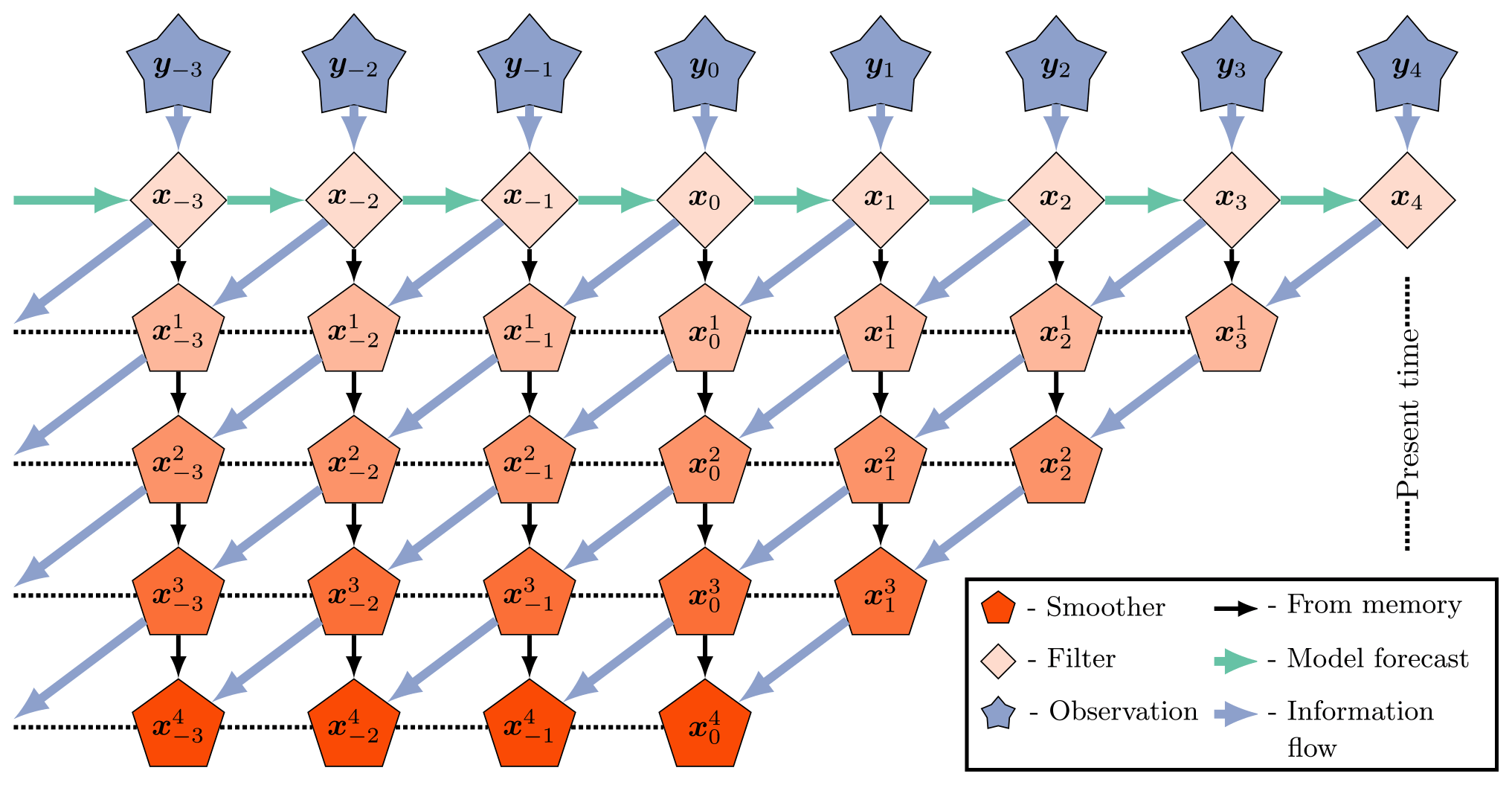
Figure 2 The EnKS with a lag =4 and a shift =1. The observations are assimilated sequentially via the filter cost function, and a retrospective reanalysis is applied to all ensemble states within the lag window stored in memory. This figure is adapted from Asch et al. (2016).

3.3 The Gauss–Newton fixed-lag IEnKS

The following is an up-to-date formulation of the Gauss–Newton IEnKS of Bocquet and Sakov (2013, 2014) and its derivations. Instead of considering the marginal smoother problem, now consider the joint posterior density directly and for a general shift S. The last posterior density is written as $p\left({\mathit{x}}_{L-S:\mathrm{1}-S}\mathrm{|}{\mathit{y}}_{L-S:\mathrm{1}-S}\right)$. Using the independence of observation errors and the Markov assumption recursively,

$$\begin{array}{ll}{\displaystyle }& {\displaystyle }p\left({\mathit{x}}_{L:\mathrm{1}}\mathrm{|}{\mathit{y}}_{L:\mathrm{1}-S}\right)\propto \\ {\displaystyle }& {\displaystyle }\int \left[\prod _{k=L-S+\mathrm{1}}^{L}p\left({\mathit{y}}_k\mathrm{|}{\mathit{x}}_k\right)p\left({\mathit{x}}_k\mathrm{|}{\mathit{x}}_{k-\mathrm{1}}\right)\right]\times \\ \text{(58)}& {\displaystyle }& {\displaystyle }\left[\prod _{k=\mathrm{1}}^{L-S}p\left({\mathit{x}}_k\mathrm{|}{\mathit{x}}_{k-\mathrm{1}}\right)\right]p\left({\mathit{x}}_{\mathrm{0}}|{\mathit{y}}_{L-S:\mathrm{1}-S}\right)\mathrm{d}{\mathit{x}}_{\mathrm{0}}.\end{array}$$

Additionally, using the perfect model assumption,

$$\begin{array}{}\text{(59)}& {\displaystyle }p\left({\mathit{x}}_k\mathrm{|}{\mathit{x}}_{k-\mathrm{1}}\right)=\mathit{\delta }\left\{{\mathit{x}}_k-{\mathcal{M}}_k\left({\mathit{x}}_{k-\mathrm{1}}\right)\right\}\end{array}$$

for every k. Therefore,

$$\begin{array}{llll}{\displaystyle }& {\displaystyle }p\left({\mathit{x}}_{L:\mathrm{1}}\mathrm{|}{\mathit{y}}_{L:\mathrm{1}-S}\right)\propto & {\displaystyle }& {\displaystyle }\int \underset{\left(\mathrm{i}\right)}{\underbrace{p\left({\mathit{x}}_{\mathrm{0}}\mathrm{|}{\mathit{y}}_{L-S:\mathrm{1}-S}\right)}}\times \\ {\displaystyle }& {\displaystyle }& {\displaystyle }& {\displaystyle }\underset{\left(\mathrm{ii}\right)}{\underbrace{\left[\prod _{k=L-S+\mathrm{1}}^{L}p\left({\mathit{y}}_k\mathrm{|}{\mathit{x}}_k\right)\right]}}\times \\ \text{(60)}& {\displaystyle }& {\displaystyle }& {\displaystyle }& {\displaystyle }\underset{\left(\mathrm{iii}\right)}{\underbrace{\left[\prod _{k=\mathrm{1}}^L\mathit{\delta }\left\{{\mathit{x}}_k-{\mathcal{M}}_k\left({\mathit{x}}_{k-\mathrm{1}}\right)\right\}\right]}}\mathrm{d}{\mathit{x}}_{\mathrm{0}},\end{array}$$

where term (i) in Eq. (60) represents the marginal smoother density for ${\mathit{x}}_{\mathrm{0}|L-S}$ over the last DAW, term (ii) represents the joint likelihood of the observations given the model state, and term (iii) represents the free forecast of the smoother estimate for ${\mathit{x}}_{\mathrm{0}|L-S}$. Noting that $p\left({\mathit{x}}_{L:\mathrm{1}}\right|{\mathit{y}}_{L:\mathrm{1}})\propto p({\mathit{x}}_{L:\mathrm{1}}\left|{\mathit{y}}_{L:\mathrm{1}-S}\right)$, this provides a recursive form to sample the joint posterior density.

Under the perfect linear Gaussian model assumption, the above derivation leads to the following exact 4D cost function:

$$\begin{array}{}\text{(61)}& {\displaystyle }\begin{array}{rl}\mathcal{J}\left({\mathit{x}}_{\mathrm{0}}\right):=& {\displaystyle \frac{\mathrm{1}}{\mathrm{2}}}\parallel {\mathit{x}}_{\mathrm{0}}-{\stackrel{\mathrm{‾}}{\mathit{x}}}_{\mathrm{0}|L-S}^{\mathrm{smth}}{\parallel }_{{\mathbf{B}}_{\mathrm{0}|L-S}^{\mathrm{smth}}}^{\mathrm{2}}+\\ & {\displaystyle \frac{\mathrm{1}}{\mathrm{2}}}\sum _{k=L-S+\mathrm{1}}^L\parallel {\mathit{y}}_k-{\mathbf{H}}_k{\mathbf{M}}_{k:\mathrm{1}}{\mathit{x}}_{\mathrm{0}}{\parallel }_{{\mathbf{R}}_k}^{\mathrm{2}}.\end{array}\end{array}$$

The ensemble-based approximation, using notations as in Eq. (41), yields the following:

$$\begin{array}{ll}\text{(62a)}& {\displaystyle }{\mathit{x}}_{\mathrm{0}}:=& {\displaystyle }{\widehat{\mathit{x}}}_{\mathrm{0}|L-S}^{\mathrm{smth}}+{\mathbf{X}}_{\mathrm{0}|L-S}^{\mathrm{smth}}\mathit{w},{\displaystyle }\stackrel{\mathrm{̃}}{\mathcal{J}}\left(\mathit{w}\right):=& {\displaystyle \frac{\mathrm{1}}{\mathrm{2}}}(N_{\mathrm{e}}-\mathrm{1})\parallel \mathit{w}{\parallel }^{\mathrm{2}}+\\ \text{(62b)}& {\displaystyle }& {\displaystyle \frac{\mathrm{1}}{\mathrm{2}}}\sum _{k=L-S+\mathrm{1}}^L\parallel {\widehat{\mathit{\delta }}}_k-{\mathbf{S}}_k\mathit{w}{\parallel }^{\mathrm{2}}.\end{array}$$

Notice that Eq. (62b) is quadratic in w; therefore, for the perfect linear Gaussian model, one can perform a global analysis over all new observations in the DAW at once.

The gradient and the Hessian of the ensemble-based 4D cost function are given as follows:

$$\begin{array}{}\text{(63a)}& {\displaystyle }\mathrm{\nabla }\stackrel{\mathrm{̃}}{\mathcal{J}}& {\displaystyle }:=(N_{\mathrm{e}}-\mathrm{1})\mathit{w}-\sum _{k=L-S+\mathrm{1}}^L{\mathbf{S}}_k^{\top }\left({\widehat{\mathit{\delta }}}_k-{\mathbf{S}}_k\mathit{w}\right),\text{(63b)}& {\displaystyle }{\stackrel{\mathrm{̃}}{\mathbf{\Xi }}}_{\stackrel{\mathrm{̃}}{\mathcal{J}}}& {\displaystyle }:=(N_{\mathrm{e}}-\mathrm{1}){\mathbf{I}}_{N_{\mathrm{e}}}+\sum _{k=L-S+\mathrm{1}}^L{\mathbf{S}}_k^{\top }{\mathbf{S}}_k,\end{array}$$

so that, evaluating at w=0, the minimizer $\widehat{\mathit{w}}$ is again given by a single iteration of Newton's descent

$$\begin{array}{}\text{(64)}& {\displaystyle }\widehat{\mathit{w}}:=\mathbf{0}-{\stackrel{\mathrm{̃}}{\mathbf{\Xi }}}_{\stackrel{\mathrm{̃}}{\mathcal{J}}}\mathrm{\nabla }\stackrel{\mathrm{̃}}{\mathcal{J}}{\mathrm{|}}_{\mathit{w}=\mathbf{0}}.\end{array}$$

Define the covariance transform again as $\mathbf{T}:={\stackrel{\mathrm{̃}}{\mathbf{\Xi }}}_{\stackrel{\mathrm{̃}}{\mathcal{J}}}^{-\frac{\mathrm{1}}{\mathrm{2}}}$. We denote the right ensemble transform corresponding to the 4D analysis ${\mathbf{\Psi }}_{L-S+\mathrm{1}:L}^{\mathrm{4}\mathrm{D}}$ to distinguish from the product of the sequential filter transforms ${\mathbf{\Psi }}_{L-S+\mathrm{1}:L}$. The global analyses are defined as follows:

$$\begin{array}{ll}{\displaystyle }\mathbf{\Psi }& {}_{L-S+\mathrm{1}:L}^{\mathrm{4}\mathrm{D}}:={\mathbf{11}}^{\top }/N_{\mathrm{e}}+\\ \text{(65a)}& {\displaystyle }& {\displaystyle }\left({\mathbf{I}}_{N_{\mathrm{e}}}-{\mathbf{11}}^{\top }/N_{\mathrm{e}}\right)\left(\widehat{\mathit{w}}{\mathbf{1}}^{\top }+\sqrt{N_{\mathrm{e}}-\mathrm{1}}\mathbf{TU}\right),\text{(65b)}& {\displaystyle }{\mathbf{E}}_{\mathrm{0}|L}^{\mathrm{smth}}& {\displaystyle }={\mathbf{E}}_{\mathrm{0}|L-S}^{\mathrm{smth}}{\mathbf{\Psi }}_{L-S+\mathrm{1}:L}^{\mathrm{4}\mathrm{D}},\end{array}$$

where U is any mean-preserving orthogonal matrix.

In the perfect linear Gaussian model, this formulation of the IEnKS is actually equivalent to the 4D-EnKF of Hunt et al. (2004), Fertig et al. (2007), and Harlim and Hunt (2007). The above scheme produces a global analysis of all observations within the DAW, even asynchronously from the standard filter cycle (Sakov et al., 2010). One generates a free ensemble forecast with the initial conditions drawn iid as $p\left({\mathit{x}}_{\mathrm{0}}\right|{\mathit{y}}_{L-S:\mathrm{1}-S})$, and all data available within the DAW are used to estimate the update to the initial ensemble. The perfect model assumption means that the updated initial ensemble ${\mathbf{E}}_{\mathrm{0}|L}^{\mathrm{smth}}$ can then be used to temporally interpolate the joint posterior estimate over the entire DAW from the marginal sample, i.e., for any $\mathrm{0}<k\le L$, a smoothing solution is defined as follows:

$$\begin{array}{}\text{(66)}& {\displaystyle }{\mathbf{M}}_{k:\mathrm{1}}{\mathbf{E}}_{\mathrm{0}|L-S}^{\mathrm{smth}}{\mathbf{\Psi }}_{L-S+\mathrm{1}:L}^{\mathrm{4}\mathrm{D}}\equiv {\mathbf{E}}_{k|L}^{\mathrm{smth}}.\end{array}$$

When ℳ_k and ℋ_k are nonlinear, the IEnKS formulation is extended with additional iterations of Newton's descent, as in Eq. (32), in order to iteratively optimize the update weights. Specifically, the gradient is given by the following:

$$\begin{array}{}\text{(67a)}& {\displaystyle }\mathrm{\nabla }\stackrel{\mathrm{̃}}{\mathcal{J}}& {\displaystyle }:=\left(N_{\mathrm{e}}-\mathrm{1}\right)\mathit{w}-\sum _{k=L-S+\mathrm{1}}^L{\stackrel{\mathrm{̃}}{\mathbf{Y}}}_k^{\top }{\mathbf{R}}_k^{-\mathrm{1}}\mathit{\phi },\text{(67b)}& {\displaystyle }\mathit{\phi }& {\displaystyle }:=\left[{\mathit{y}}_k-{\mathcal{H}}_k\circ {\mathcal{M}}_{k:\mathrm{1}}\left({\widehat{\mathit{x}}}_{\mathrm{0}|L-S}^{\mathrm{smth}}+{\mathbf{X}}_{\mathrm{0}|L-S}^{\mathrm{smth}}\mathit{w}\right)\right],\end{array}$$

where ${\stackrel{\mathrm{̃}}{\mathbf{Y}}}_k$ represents a directional derivative of the observation and state models with respect to the ensemble perturbations at the ensemble mean, as follows:

$$\begin{array}{}\text{(68)}& {\displaystyle }{\stackrel{\mathrm{̃}}{\mathbf{Y}}}_k:=\mathrm{\nabla }{\mathrm{|}}_{{\widehat{\mathit{x}}}_{\mathrm{0}|L-S}^{\mathrm{smth}}}\left[{\mathcal{H}}_k\circ {\mathcal{M}}_{k:\mathrm{1}}\right]{\mathbf{X}}_{\mathrm{0}|L-S}^{\mathrm{smth}}.\end{array}$$

This describes the sensitivities of the cost function, with respect to the ensemble perturbations, mapped to the observation space. When the dynamics is weakly nonlinear, the ensemble perturbations of the EnKS and IEnKS are known to closely align with the span of the backward Lyapunov vectors of the nonlinear model along the true state trajectory (Bocquet and Carrassi, 2017). Under these conditions, Eq. (68) can be interpreted as a directional derivative with respect to the forecast error growth along the dynamical instabilities of the nonlinear model (see Carrassi et al., 2022, and references therein).

In order to avoid an explicit computation of the tangent linear model and the adjoint as in 4D-Var, Sakov et al. (2012) and Bocquet and Sakov (2012) proposed two formulations to approximate the tangent linear propagation of the ensemble perturbations. The bundle scheme makes an explicit approximation of finite differences in the observation space where, for an arbitrary ensemble, they define the approximate linearization as follows:

$$\begin{array}{}\text{(69)}& {\displaystyle }{\mathbf{Y}}_k:={\displaystyle \frac{\mathrm{1}}{\mathit{ϵ}}}{\mathcal{H}}_k\circ {\mathcal{M}}_{k:\mathrm{1}}\left({\mathit{x}}_{\mathrm{0}}{\mathbf{1}}^{\top }+\mathit{ϵ}{\mathbf{X}}_{\mathrm{0}}\right)\left({\mathbf{I}}_{N_{\mathrm{e}}}-{\mathbf{11}}^{\top }/N_{\mathrm{e}}\right),\end{array}$$

for a small constant ϵ. Alternatively, the transform version provides a different approximation to the variational analysis, using the covariance transform T and its inverse as a pre-/post-conditioning of the perturbations used in the sensitivities approximation. The transform variant of the IEnKS is in some cases more numerically efficient than the bundle version, requiring fewer ensemble simulations, and it is explicitly related to the ETKF/EnKS/4D-EnKF formalism presented thus far. For these reasons, the transform approximation is used as a basis of comparison with the other schemes in this work.

For the IEnKS transform variant, the ensemble-based approximations are redefined in each Newton iteration as follows:

$$\begin{array}{}\text{(70a)}& {\displaystyle }{\mathbf{Y}}_k& {\displaystyle }:={\mathcal{H}}_k\left({\mathbf{E}}_k\right),\text{(70b)}& {\displaystyle }{\widehat{\mathit{y}}}_k& {\displaystyle }:={\mathbf{Y}}_k\mathbf{1}/N_{\mathrm{e}},\text{(70c)}& {\displaystyle }{\mathbf{S}}_k& {\displaystyle }:={\mathbf{R}}_k^{-\frac{\mathrm{1}}{\mathrm{2}}}\left({\mathbf{Y}}_k-{\widehat{\mathit{y}}}_k{\mathbf{1}}^{\top }\right){\mathbf{T}}^{-\mathbf{1}},\text{(70d)}& {\displaystyle }\widehat{\mathit{\delta }}& {\displaystyle }:={\mathbf{R}}_k^{-\frac{\mathrm{1}}{\mathrm{2}}}\left({\mathit{y}}_k-{\widehat{\mathit{y}}}_k\right),\end{array}$$

where the first covariance transform is defined as $\mathbf{T}:={\mathbf{I}}_{N_{\mathrm{e}}}$, the gradient and Hessian are computed as in Eq. (63) from the above, and where the covariance transform is redefined in terms of the Hessian, $\mathbf{T}:={\stackrel{\mathrm{̃}}{\mathbf{\Xi }}}_{\stackrel{\mathrm{̃}}{\mathcal{J}}}^{-\frac{\mathrm{1}}{\mathrm{2}}}$, at the end of each iteration. With these definitions, the first iteration of the IEnKS transform variant corresponds to the solution of the nonlinear 4D-EnKF, but subsequent iterates are initialized by pre-conditioning the initial ensemble perturbations via the update T and post-conditioning the sensitivities by the inverse transform T⁻¹.

An updated form of the Gauss–Newton IEnKS transform variant is presented in Algorithm A7. Note that, while Algorithm A7 does not explicitly reference the sub-routine in Algorithm A1, many of the same steps are used in the IEnKS when computing the sensitivities. It is important to notice that, for S>1, the IEnKS only requires a single computation of the square root inverse of the Hessian of the 4D cost function, per iteration of the optimization, to process all observations in the DAW. On the other hand, the EnKS processes these observations sequentially, requiring S total square root inverse calculations of the Hessian, corresponding to each of the sequential filter cost functions.

The IEnKS is computationally constrained by the fact that each iteration of the descent requires L total ensemble simulations in the dynamical state model ℳ_k. One can minimize this expense by using a single iteration of the IEnKS equations, which is denoted the linearized IEnKS (Lin-IEnKS) by Bocquet and Sakov (2014). When the overall DA cycle is nonlinear, but only weakly nonlinear, this single iteration of the IEnKS algorithm can produce a dramatic improvement in the forecast accuracy versus the forecast/filter cycle of the EnKS. However, the overall nonlinearity of the DA cycle may be strongly influenced by factors other than the model forecast ℳ_k itself. As a simple example, consider the case in which ℋ_k is nonlinear yet ℳ_k≡M_k for all k. In this setting, it may be more numerically efficient to iterate upon the 3D filter cost function rather than the full 4D cost function which requires simulations of the state model. Combining (i) the filter step and retrospective reanalysis of the EnKS and (ii) the single iteration of the ensemble simulation over the DAW as in Lin-IEnKS, we obtain an estimation scheme that sequentially solves the nonlinear filter cost functions in the current DAW, while making an improved forecast in the next by transmitting the retrospective analyses through the dynamics via the updated initial ensemble.

3.4 The fixed-lag SIEnKS

3.4.1 Algorithm

Recall that, from Eq. (57), conditioning the ensemble with the right transform Ψ_k is covariant with the dynamics. In a perfect linear Gaussian model, we can therefore estimate the joint posterior over the DAW via model propagation of the marginal for ${\mathit{x}}_{\mathrm{0}|L}^{\mathrm{smth}}$, as in the IEnKS but by using the EnKS retrospective reanalysis to generate the initial condition. For arbitrary $\mathrm{1}\le S\le L$, define each of the right transforms ${\left\{{\mathbf{\Psi }}_k\right\}}_{k=L-S+\mathrm{1}}^L$ as in the sequential filter analysis of the ETKF with Eq. (45). Rather than storing the ensemble matrix in memory for each time t_k in the DAW, we instead store ${\mathbf{E}}_{\mathrm{0}|L-S}^{\mathrm{smth}}$ and ${\mathbf{E}}_{L-S|L-S}^{\mathrm{smth}}$ to begin a DA cycle. Observations within the DAW are sequentially assimilated via the 3D filter cycle initialized with ${\mathbf{E}}_{L-S|L-S}^{\mathrm{smth}}$ and a marginal, retrospective, smoother analysis is performed sequentially on ${\mathbf{E}}_{\mathrm{0}|L-S}^{\mathrm{smth}}$ with these filter transforms. The joint posterior estimate is then interpolated over the DAW for any $\mathrm{1}\le k\le L$ via the model dynamics as follows:

$$\begin{array}{}\text{(71a)}& {\displaystyle }{\mathbf{E}}_{\mathrm{0}|L}^{\mathrm{smth}}& {\displaystyle }={\mathbf{E}}_{\mathrm{0}|L-S}^{\mathrm{smth}}{\mathbf{\Psi }}_{L-S+\mathrm{1}:L},\text{(71b)}& {\displaystyle }{\mathbf{E}}_{k|L}^{\mathrm{smth}}& {\displaystyle }:={\mathcal{M}}_{k:\mathrm{1}}\left({\mathbf{E}}_{\mathrm{0}|L}^{\mathrm{smth}}\right).\end{array}$$

Notice that, for S=1, the product of the 3D filter ensemble transforms reduces to the 4D transform, i.e.,

$$\begin{array}{}\text{(72)}& {\displaystyle }{\mathbf{\Psi }}_{L-S+\mathrm{1}:L}\equiv {\mathbf{\Psi }}_{L-S+\mathrm{1}:L}^{\mathrm{4}\mathrm{D}}\equiv {\mathbf{\Psi }}_L,\end{array}$$

so that, in the perfect linear Gaussian model with S=1, the SIEnKS and the Lin-IEnKS coincide. The SIEnKS and the Lin-IEnKS have different treatments of nonlinearity in the DA cycle, but even in the perfect linear Gaussian model, a shift S>1 distinguishes the 4D approach of the Lin-IEnKS and the hybrid 3D/4D approach of the SIEnKS. For comparison, a schematic of the SIEnKS cycle is pictured in Fig. 3, while a schematic of the (Lin-)IEnKS cycle is shown in Fig. 4, and each is configured for a lag of L=4 and a shift of S=2. This comparison demonstrates how the sequential 3D filter analysis and retrospective smoother reanalysis for each observation differ from the global 4D analysis of all observations at once in the (Lin-)IEnKS. A generic form of the SIEnKS is summarized in Algorithm A8, utilizing the sub-routines in Algorithms A1–A4. Note that the version presented in Algorithm A8 is used to emphasize the commonality with the EnKS. However, an equivalent implementation initializes each cycle with ${\mathbf{E}}_{\mathrm{0}|L-S}^{\mathrm{smth}}$ alone, similar to the IEnKS. Such a design is utilized when we derive the SIEnKS MDA scheme in Algorithm A12 from the IEnKS MDA scheme in Algorithm A13.

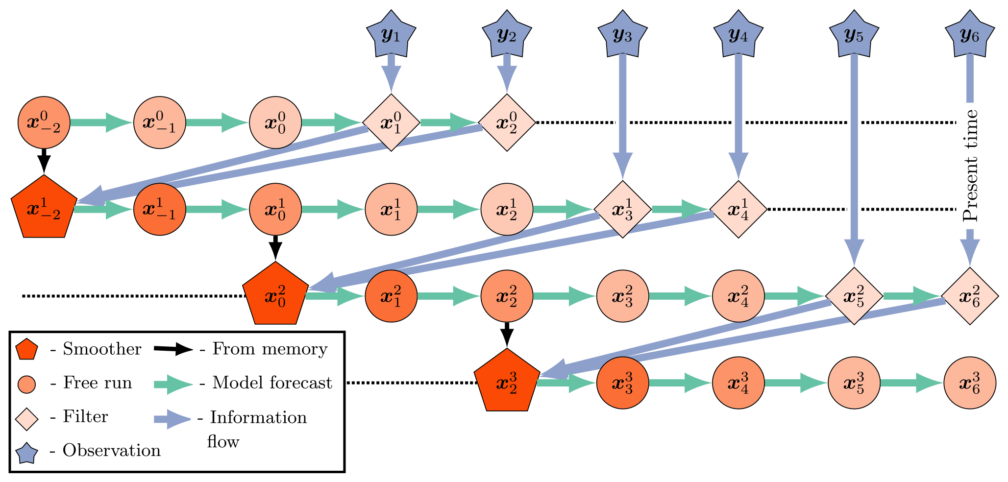
Figure 3 The SIEnKS with a lag =4 and a shift =2. An initial condition from the last smoothing cycle initializes a forecast simulation over the current DAW of the L=4 states. New observations entering the DAW are assimilated sequentially via the 3D filter cost function. After each filter analysis, a retrospective reanalysis is applied to the initial ensemble. At the end of the DAW, after sequentially processing all observations, the reanalyzed initial condition is evolved, via the model S analysis times, forward to begin the next cycle.

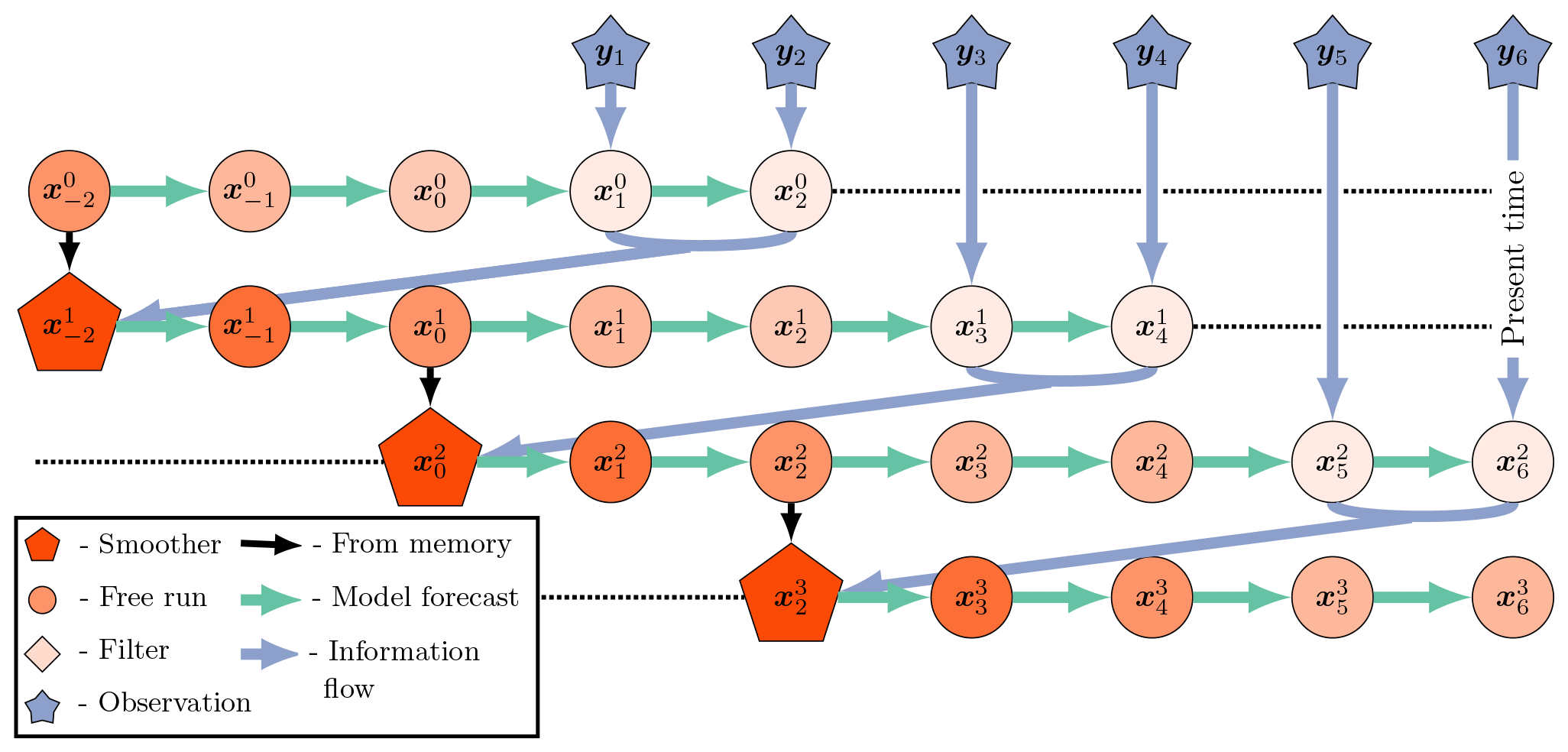
Figure 4 The (Lin-)IEnKS with a lag =4 and a shift =2. An initial condition from the last smoothing cycle initializes a forecast simulation over the current DAW of the L=4 states. Unlike the SIEnKS, all new observations entering the DAW are assimilated globally at once via the 4D cost function. The innovations of the free forecast over all of the observation times are used to produce a retrospective reanalysis of the initial ensemble. Finally, the reanalyzed initial condition is evolved, via the model, S analysis times forward to begin the next cycle. Unlike the SIEnKS and the EnKS, the filter analysis of the (Lin-)IEnKS is performed by dynamically interpolating the smoothing estimate over new observation times with a free forecast in the subsequent cycle. The Lin-IEnKS is differentiated from the IEnKS by using only a single free ensemble forecast to produce the 4D optimization of the initial ensemble in each cycle.

3.4.2 Comparison with other schemes

Other well-known DA schemes combining a retrospective reanalysis and reinitialization of the ensemble forecast include the running-in-place (RIP) smoother of Kalnay and Yang (2010) and the one-step-ahead (OSA) smoother of Desbouvries et al. (2011) and Ait-El-Fquih and Hoteit (2022). The RIP smoother iterates over both the ensemble simulation and filter cost function, in order to apply a retrospective reanalysis to the first prior with a lag and shift of $L=S=\mathrm{1}$. The RIP smoother is designed to spin up the LETKF from a cold start of a forecast model and DA cycle (Yang et al., 2013). However, the RIP optimizes a different style cost function than the S/Lin-/IEnKS family of smoothers. The stopping criterion for RIP is formulated in terms of the mean square distance between the ensemble forecast and the observation, potentially leading to an overfitting of the observation. The OSA smoother is also proposed as an optimization of the DA cycle and integrates an EnKF framework, including for a two-stage, iterative optimization of dynamical forecast model parameters within the DA cycle (Gharamti et al., 2015; Ait-El-Fquih et al., 2016; Raboudi et al., 2018). The OSA smoother uses a single iteration and a lag and shift of $L=S=\mathrm{1}$, making a filter analysis of the incoming observation and a retrospective reanalysis of the prior. However, the OSA smoother differs from the SIEnKS in using an additional filter analysis while interpolating the joint posterior estimate over the DAW, accounting for model error in the simulation of ${\mathcal{M}}_{\mathrm{1}}\left({\mathbf{E}}_{\mathrm{0}|\mathrm{1}}^{\mathrm{smth}}\right)$. Without model error, the second filter analysis in the OSA smoother simulation is eliminated from the estimation scheme. Therefore, with an ETKF-style filter analysis, a perfect linear Gaussian model and a lag of $L=S=\mathrm{1}$, the SIEnKS, and RIP and OSA smoothers all coincide.

The rationale for the SIEnKS is to focus computational resources on optimizing the sequence of 3D filter cost functions for the DAW when the forecast error dynamics is weakly nonlinear, rather than computing the iterative ensemble simulations needed to optimize a 4D cost function. The SIEnKS generalizes some of the ideas used in these other DA schemes, particularly for perfect models with weakly nonlinear forecast error dynamics, including for (i) arbitrary lags and shifts $\mathrm{1}\le S\le L$, (ii) an iterative optimization of hyperparameters for the filter cost function, (iii) multiple data assimilation, and (iv) asynchronous observations in the DA cycle. In order to illustrate the novelty of the SIEnKS, and to motivate its computational cost/prediction accuracy tradeoff advantages, we discuss each of these topics in the following.

4 Applications of single-iteration smoothing

4.1 Nonlinear observation operators

Just as the IEnKS extends the linear 4D cost function, the filter cost function in Eq. (42) can be extended with Newton iterates in the presence of a nonlinear observation operator. The maximum likelihood ensemble filter (MLEF) of Zupanski (2005) and Zupanski et al. (2008) is an estimator designed to process nonlinear observation operators and can be derived in the common ETKF formalism. Particularly, the algorithm can be granted bundle and transform variants like the IEnKS (Asch et al., 2016; see Sect. 6.7.2.1), which are designed to approximate the directional derivative of the nonlinear observation operator with respect to the forecast ensemble perturbations at the forecast mean,

$$\begin{array}{}\text{(73)}& {\displaystyle }{\stackrel{\mathrm{̃}}{\mathbf{Y}}}_k:=\mathrm{\nabla }{\mathrm{|}}_{{\widehat{\mathit{x}}}_k^{\mathrm{fore}}}\left[{\mathcal{H}}_k\right]{\mathbf{X}}_k^{\mathrm{fore}},\end{array}$$

which is used in the nonlinear filter cost function gradient as follows:

$$\begin{array}{ll}{\displaystyle }\mathrm{\nabla }\stackrel{\mathrm{̃}}{\mathcal{J}}:=& {\displaystyle }\left(N_{\mathrm{e}}-\mathrm{1}\right)\mathit{w}-\\ \text{(74)}& {\displaystyle }& {\displaystyle }{\stackrel{\mathrm{̃}}{\mathbf{Y}}}_k^{\top }{\mathbf{R}}_k^{-\mathrm{1}}\left[{\mathit{y}}_k-{\mathcal{H}}_k\left({\widehat{\mathit{x}}}_k^{\mathrm{fore}}+{\mathbf{X}}_k^{\mathrm{fore}}\mathit{w}\right)\right].\end{array}$$

When the forecast error dynamics is weakly nonlinear, the MLEF-style nonlinear filter cost function optimization provides a direct extension to the SIEnKS. The transform, as defined in the sub-routine in Algorithm A9, is interchangeable with the usual ensemble transform in Algorithm A1. In this way, the EnKS and the SIEnKS can each process nonlinear observation operators with an iterative optimization in the filter cost function alone and, subsequently, apply their retrospective analyses as usual. We refer to the EnKS analysis with MLEF transform as the maximum likelihood ensemble smoother (MLES), though we refer to the SIEnKS as usual, whether it uses a single iteration or multiple iterations of the solution to the filter cost function. Note that only the transform step needs to be interchanged in Algorithms A6 and A8, so we do not provide additional pseudo-code.

Consider that, for the MLES and the SIEnKS, the number of Hessian square root inverse calculations expands in the number of iterations used in Algorithm A9 to compute the transform for each of the S observations in the DAW. For each iteration of the IEnKS, this again requires only a single square root inverse calculation of the 4D cost function Hessian. However, even if the forecast error dynamics is weakly nonlinear, optimizing versus the nonlinear observation operator requires L ensemble simulations for each iteration used to optimize the cost function.

4.2 Adaptive inflation and the finite size formalism

Due to the bias of Kalman-like estimators in nonlinear dynamics, covariance inflation, as in Algorithm A4, is widely used to regularize these schemes. In particular, this can ameliorate the systematic underestimation of the prediction/posterior uncertainty due to sample error and bias. Empirically tuning the multiplicative inflation coefficient λ≥1 can be effective in stationary dynamics. However, empirically tuning this parameter can be costly, potentially requiring many model simulations, and the tuned value may not be optimal across timescales in which the dynamical system becomes non-stationary. A variety of techniques is used in practice for adaptive covariance estimation, inflation, or augmentation, accounting for these deficiencies of the Kalman-like estimators (Tandeo et al., 2020, and references therein).

One alternative to empirically tuning λ is to derive an adaptive multiplicative covariance inflation factor via a hierarchical Bayesian model by including a prior on the background mean and covariance $p\left({\stackrel{\mathrm{‾}}{\mathit{x}}}_{\mathrm{1}}^{\mathrm{fore}},{\mathbf{B}}_{\mathrm{1}}^{\mathrm{fore}}\right)$, as in the finite size formalism of Bocquet (2011), Bocquet and Sakov (2012), and Bocquet et al. (2015). This formalism seeks to marginalize out over the first 2 moments of the background, yielding a Gaussian mixture model for the forecast prior as follows:

$$\begin{array}{llll}{\displaystyle }& {\displaystyle }p\left({\mathit{x}}_{\mathrm{1}}|{\mathbf{E}}_{\mathrm{1}}^{\mathrm{fore}}\right)& {\displaystyle }=\int & {\displaystyle }p\left({\mathit{x}}_{\mathrm{1}}|{\mathbf{E}}_{\mathrm{1}}^{\mathrm{fore}},{\stackrel{\mathrm{‾}}{\mathit{x}}}_{\mathrm{1}}^{\mathrm{fore}},{\mathbf{B}}_{\mathrm{1}}^{\mathrm{fore}}\right)\times \\ \text{(75)}& {\displaystyle }& {\displaystyle }& {\displaystyle }& {\displaystyle }p\left({\stackrel{\mathrm{‾}}{\mathit{x}}}_{\mathrm{1}}^{\mathrm{fore}},{\mathbf{B}}_{\mathrm{1}}^{\mathrm{fore}}|{\mathbf{E}}_{\mathrm{1}}^{\mathrm{fore}}\right)\mathrm{d}{\stackrel{\mathrm{‾}}{\mathit{x}}}_{\mathrm{1}}^{\mathrm{fore}}\mathrm{d}{\mathbf{B}}_{\mathrm{1}}^{\mathrm{fore}}.\end{array}$$

Using Jeffreys' hyperprior for ${\stackrel{\mathrm{‾}}{\mathit{x}}}_{\mathrm{1}}^{\mathrm{fore}}$ and ${\mathbf{B}}_{\mathrm{1}}^{\mathrm{fore}}$, the ensemble-based filter MAP cost function can be derived as proportional to the following:

$$\begin{array}{ll}{\displaystyle }\stackrel{\mathrm{̃}}{\mathcal{J}}\left(\mathit{w}\right):=& {\displaystyle \frac{\mathrm{1}}{\mathrm{2}}}\parallel \mathit{y}-\mathcal{H}\left({\widehat{\mathit{x}}}_{\mathrm{1}}^{\mathrm{fore}}+{\mathbf{X}}_{\mathrm{1}}^{\mathrm{fore}}\mathit{w}\right){\parallel }_{{\mathbf{R}}_{\mathrm{1}}}^{\mathrm{2}}+\\ \text{(76)}& {\displaystyle }& {\displaystyle \frac{N_{\mathrm{e}}}{\mathrm{2}}}\log \left({\mathit{ϵ}}_{N_{\mathrm{e}}}+\parallel \mathit{w}{\parallel }^{\mathrm{2}}\right),\end{array}$$

where ${\mathit{ϵ}}_{N_{\mathrm{e}}}:=\mathrm{1}+\frac{\mathrm{1}}{N_{\mathrm{e}}}$. Notice that Eq. (76) is non-quadratic in w, regardless of whether ℋ₁ is linear or nonlinear, such that one can iteratively optimize the solution to the nonlinear filter cost function with a Gauss–Newton approximation of the descent. When accounting for the nonlinearity in the ensemble evolution and the sample error due to small ensemble sizes in perfect models, optimizing the extended cost function in Eq. (76) can be an effective means to regularize the EnKF. In the presence of significant model error, one may need to extend the finite size formalism to the variant developed by Raanes et al. (2019a).

Algorithm A10 presents an updated version of the finite size ensemble Kalman filter (EnKF-N) transform calculation of Bocquet et al. (2015), explicitly based on the IEnKS transform approximation of the gradient of the observation operator. The hyperprior for the background mean and covariance is similarly introduced to the IEnKS and optimized over an extended 4D cost function. Note that, in the case when ℋ_k≡H_k is linear, a dual, scalar optimization can be performed for the filter cost function with less numerical expense. However, there is no similar reduction to the extended 4D cost function, and in order to emphasize the structural difference between the 4D approach and the sequential approach, we focus on the transform variant analogous to the IEnKS optimization.

Extending the adaptive covariance inflation in the finite size formalism to either the EnKS or the SIEnKS is simple, requiring that the ensemble transform calculation is interchanged with Algorithm A10 and that the tuned multiplicative inflation step is eliminated. The finite size iterative ensemble Kalman smoother (IEnKS-N) transform variant, including adaptive inflation as above, is described in Algorithm A11. Notice that iteratively optimizing the inflation hyperparameter comes at the additional expense of square root inverse Hessian calculations for the EnKS and the SIEnKS, while the IEnKS also requires L additional ensemble simulations for each iteration.

4.3 Multiple data assimilation

When the lag L>1 is long, temporally interpolating the posterior estimate in the DAW via the nonlinear model solution, as in Eq. (71), becomes increasingly nonlinear. In chaotic dynamics, the small simulation errors introduced this way eventually degrade the posterior estimate, and this interpolation becomes unstable when L is taken to be sufficiently large. Furthermore, for the 4D cost function, observations only distantly connected with the initial condition at the beginning of the DAW render the cost function with more local minima that may strongly affect the performance of the optimization. Multiple data assimilation is a commonly used technique, based on statistical tempering (Neal, 1996), designed to relax the nonlinearity of performing the MAP estimate by artificially inflating the variances of the observation errors with weights and assimilating these observations multiple times. Multiple data assimilation is made consistent with the Bayesian posterior in perfect linear Gaussian models by appropriately choosing weights so that, over all times that an observation vector is assimilated, all of its associated weights sum to one (Emerick and Reynolds, 2013). Given Gaussian likelihood functions, this implies that the sum of the precision matrices over the multiple assimilation steps equals R⁻¹, as with the usual Kalman filter update.

Multiple data assimilation is integrated into the EnRML for static DAWs in reservoir modeling (Evensen, 2018, and references therein). With the fixed-lag, sequential EnKS, there is no reason to perform MDA as the assimilation occurs in a single pass over each observation with the filter step as in the ETKF. Sequential MDA, with DAWs shifting in time, was first derived with the IEnKS by Bocquet and Sakov (2014). In order to sample the appropriate density, the IEnKS MDA estimation is broken over two stages. First, in the balancing stage, the IEnKS fully assimilates all partially assimilated observations, targeting the joint posterior statistics. Second, the window of the partially assimilated observations is shifted in time with the MDA stage. The SIEnKS is similarly broken over these two stages, using the same weights as the IEnKS above. However, there is an important difference in the way MDA is formulated for the SIEnKS versus the IEnKS. For the SIEnKS, each observation in the DAW is assimilated with the sequential 3D filter cost function instead of the global 4D analysis in the IEnKS. The sequential filter analysis constrains the posterior's interpolation estimate to the observations in the balancing stage, as observations are assimilated sequentially in the SIEnKS, whereas the posterior estimate is performed by interpolating with a free forecast from the marginal posterior estimate in the IEnKS. Our novel SIEnKS MDA scheme is derived as follows.

Recall our algorithmically stationary DAW, $\mathit{\{}{t}_{\mathrm{1}},\mathrm{\cdots },t_L\mathit{\}}$, and suppose, at the moment, that there is a shift of S=1 and an arbitrary lag L. We take the notation that the covariance matrices for the likelihood functions are inflated to be as follows:

$$\begin{array}{}\text{(77)}& {\displaystyle }p\left({\mathit{y}}^{\mathit{\beta }}\mathrm{|}\mathit{x}\right):=n\left(\mathit{y}\mathrm{|}\mathcal{H}\left(\mathit{x}\right),{\mathit{\beta }}^{-\mathrm{1}}\mathbf{R}\right),\end{array}$$

where the observation weights are assumed $\mathrm{0}<\mathit{\beta }\le \mathrm{1}$. We index the weight for observation y_k at the present time t_L as β_k|L. For consistency with the perfect linear Gaussian model, we require that

$$\begin{array}{}\text{(78)}& {\displaystyle }\sum _{i=\mathrm{1}}^L{\mathit{\beta }}_{i|L}=\mathrm{1}.\end{array}$$

This implies that, as we assimilate an observation vector for L total times, shifting the algorithmically stationary DAW, the sum of the weights used to assimilate the observation equals one.

We denote

$$\begin{array}{}\text{(79)}& {\displaystyle }{\mathit{\alpha }}_{k|L}:=\sum _{i=k}^L{\mathit{\beta }}_{i|L}\end{array}$$

as the fraction of the observation y_k that has been assimilated after the analysis step at the time t_L. Note that, under the Gaussian likelihood assumption, and assuming the independence of the fractional observations, this implies that

$$\begin{array}{}\text{(80)}& {\displaystyle }\prod _{i=k}^{L}p\left({\mathit{y}}^{{\mathit{\beta }}_{i|L}}\mathrm{|}\mathit{x}\right)=p\left({\mathit{y}}^{{\mathit{\alpha }}_{k|L}}\mathrm{|}\mathit{x}\right).\end{array}$$

Let ${\mathit{\beta }}_{l:k|L}$ and ${\mathit{\alpha }}_{l:k|L}$ denote the length $(l-k+\mathrm{1})$ vectors as follows:

$$\begin{array}{}\text{(81a)}& {\displaystyle }{\mathit{\beta }}_{l:k|L}& {\displaystyle }=\left(\begin{array}{ccc}{\mathit{\beta }}_{l|L}& \mathrm{\cdots }& {\mathit{\beta }}_{k|L}\end{array}\right),\text{(81b)}& {\displaystyle }{\mathit{\alpha }}_{l:k|L}& {\displaystyle }=\left(\begin{array}{ccc}{\mathit{\alpha }}_{l|L}& \mathrm{\cdots }& {\mathit{\alpha }}_{k|L}\end{array}\right).\end{array}$$

We then define the sequences,

$$\begin{array}{}\text{(82a)}& {\displaystyle }{\mathit{y}}_{l:k}^{{\mathit{\beta }}_{l:k|L}}& {\displaystyle }:=\left\{{\mathit{y}}_l^{{\mathit{\beta }}_{l|L}},{\mathit{y}}_{l-\mathrm{1}}^{{\mathit{\beta }}_{l-\mathrm{1}|L}},\mathrm{\cdots },{\mathit{y}}_k^{{\mathit{\beta }}_{k|L}}\right\},\text{(82b)}& {\displaystyle }{\mathit{y}}_{l:k}^{{\mathit{\alpha }}_{l:k|L}}& {\displaystyle }:=\left\{{\mathit{y}}_l^{{\mathit{\alpha }}_{l:L}},{\mathit{y}}_{l-\mathrm{1}}^{{\mathit{\alpha }}_{l-\mathrm{1}|L}},\mathrm{\cdots },{\mathit{y}}_k^{{\mathit{\alpha }}_{k|l}}\right\},\end{array}$$

as the observations y_l:k in the current DAW $\mathit{\{}{t}_{\mathrm{1}},\mathrm{\cdots },t_L\mathit{\}}$, with Eq. (82a), the corresponding MDA weights for this DAW, and, with Eq. (82b), the total portion of each observation assimilated in the MDA conditional density for this DAW after the analysis step. Similar definitions apply with the indices $l:k|L-\mathrm{1}$ but are relative to the previous DAW.

For the current DAW, the balancing stage is designed to sample the joint posterior density,

$$\begin{array}{}\text{(83)}& {\displaystyle }p\left({\mathit{x}}_{L:\mathrm{1}}\mathrm{|}{\mathit{y}}_{L:\mathrm{1}}\right),\end{array}$$

where the current cycle is initialized with a sample of the MDA conditional density,

$$\begin{array}{}\text{(84)}& {\displaystyle }p\left({\mathit{x}}_{\mathrm{0}}\mathrm{|}{\mathit{y}}_{L-\mathrm{1}:\mathrm{0}}^{{\mathit{\alpha }}_{L-\mathrm{1}:\mathrm{0}|L-\mathrm{1}}}\right).\end{array}$$

That is, from the previous cycle, we have a marginal estimate for x₀, given the sequence of observations ${\mathit{y}}_{L-\mathrm{1}:\mathrm{0}}$, where the portion of observation y_k that has been assimilated already is given by ${\mathit{\alpha }}_{k|L-\mathrm{1}}$. Notice that ${\mathit{\alpha }}_{\mathrm{0}|L-\mathrm{1}}=\mathrm{1}$ so that y₀ has already been fully assimilated. To fully assimilate y₁, we note that $\mathrm{1}-{\mathit{\alpha }}_{\mathrm{1}|L-\mathrm{1}}={\mathit{\beta }}_{\mathrm{1}|L}$, and therefore,

$$\begin{array}{ll}{\displaystyle }p\left({\mathit{x}}_{\mathrm{1}:\mathrm{0}}|{\mathit{y}}_{L-\mathrm{1}:\mathrm{2}}^{{\mathit{\alpha }}_{L-\mathrm{1}:\mathrm{2}|L-\mathrm{1}}},{\mathit{y}}_{\mathrm{1}:\mathrm{0}}\right)\propto & {\displaystyle }p\left({\mathit{y}}_{\mathrm{1}}^{{\mathit{\beta }}_{\mathrm{1}|L}}|{\mathit{x}}_{\mathrm{1}}\right)p\left({\mathit{x}}_{\mathrm{1}}|{\mathit{x}}_{\mathrm{0}}\right)\times \\ \text{(85)}& {\displaystyle }& {\displaystyle }p\left({\mathit{x}}_{\mathrm{0}}\mathrm{|}{\mathit{y}}_{L-\mathrm{1}:\mathrm{0}}^{{\mathit{\alpha }}_{L-\mathrm{1}:\mathrm{0}|L-\mathrm{1}}}\right).\end{array}$$

The above corresponds to a single simulation/analysis step in an EnKS cycle, where the observation ${\mathit{y}}_{\mathrm{1}}^{{\mathit{\beta }}_{\mathrm{1}|L}}$ is assimilated, and a retrospective reanalysis is applied to the ensemble at t₀.

More generally, to fully assimilate observation y_k, we assimilate the remaining portion left unassimilated from the last DAW and given as $\mathrm{1}-{\mathit{\alpha }}_{k|L-\mathrm{1}}$. We define an inductive step describing the density for x_k:0, which has fully assimilated y_k:0, though it has yet to assimilate the remaining portions of observations ${\mathit{y}}_{L-\mathrm{1}:k+\mathrm{1}}$, as follows:

$$\begin{array}{}\text{(86)}& {\displaystyle }\begin{array}{rl}p({\mathit{x}}_{k:\mathrm{0}}& |{\mathit{y}}_{L-\mathrm{1}:k+\mathrm{1}}^{{\mathit{\alpha }}_{L-\mathrm{1}:k+\mathrm{1}|L-\mathrm{1}}},{\mathit{y}}_{k:\mathrm{0}})\propto p\left({\mathit{y}}_k^{\mathrm{1}-{\mathit{\alpha }}_{k|L-\mathrm{1}}}|{\mathit{x}}_k\right)\times \\ & p\left({\mathit{x}}_k\right|{\mathit{x}}_{k-\mathrm{1}})p\left({\mathit{x}}_{k-\mathrm{1}:\mathrm{0}}|{\mathit{y}}_{L-\mathrm{1}:k}^{{\mathit{\alpha }}_{L-\mathrm{1}:k|L-\mathrm{1}}},{\mathit{y}}_{k-\mathrm{1}:\mathrm{0}}\right).\end{array}\end{array}$$

For $k=\mathrm{2},\mathrm{\cdots },L-\mathrm{2}$, this describes a subsequent simulation/analysis step of an EnKS cycle but where the observation ${\mathit{y}}_k^{\mathrm{1}-{\mathit{\alpha }}_{k|L-\mathrm{1}}}$ is assimilated and a retrospective analysis is applied to the ensemble at times $t_{\mathrm{0}},\mathrm{\cdots },t_{k-\mathrm{1}}$. A subsequent EnKS analysis gives the following:

$$\begin{array}{}\text{(87)}& {\displaystyle }\begin{array}{rl}p({\mathit{x}}_{L-\mathrm{1}:\mathrm{0}}& \left|{\mathit{y}}_{L-\mathrm{1}:\mathrm{0}}\right)\propto p\left({\mathit{y}}_{L-\mathrm{1}}^{\mathrm{1}-{\mathit{\alpha }}_{L-\mathrm{1}|L-\mathrm{1}}}|{\mathit{x}}_{L-\mathrm{1}}\right)\times \\ & p\left({\mathit{x}}_{L-\mathrm{1}}\right|{\mathit{x}}_{L-\mathrm{2}})p\left({\mathit{x}}_{L-\mathrm{2}:\mathrm{0}}|{\mathit{y}}_{L-\mathrm{1}}^{{\mathit{\alpha }}_{L-\mathrm{1}|L-\mathrm{1}}},{\mathit{y}}_{L-\mathrm{2}:\mathrm{0}}\right),\end{array}\end{array}$$

i.e., this samples the joint posterior for the last DAW. A final EnKS analysis is used to assimilate y_L, for which no portion was already assimilated in the previous DAW, as follows:

$$\begin{array}{}\text{(88)}& {\displaystyle }\begin{array}{rl}p\left({\mathit{x}}_{L:\mathrm{1}}\right|{\mathit{y}}_{L:\mathrm{1}})\propto & p\left({\mathit{y}}_L\right|{\mathit{x}}_L)\times \\ & p\left({\mathit{x}}_L\right|{\mathit{x}}_{L-\mathrm{1}}\left)p\right({\mathit{x}}_{L-\mathrm{1}:\mathrm{0}}\left|{\mathit{y}}_{L-\mathrm{1}:\mathrm{0}}\right).\end{array}\end{array}$$

We thus define an initial ensemble, distributed approximately as follows:

$$\begin{array}{}\text{(89)}& {\displaystyle }{\mathbf{E}}_{\mathrm{0}}^{\mathrm{bal}}\sim p\left({\mathit{x}}_{\mathrm{0}}|{\mathit{y}}_{L-\mathrm{1}:\mathrm{0}}^{{\mathit{\alpha }}_{L-\mathrm{1}:\mathrm{0}|L-\mathrm{1}}}\right).\end{array}$$

In the balancing stage, the observation error covariance weights are defined by the following:

$$\begin{array}{}\text{(90)}& {\displaystyle }{\mathit{\eta }}_{k|L}:=\mathrm{1}-{\mathit{\alpha }}_{k|L-\mathrm{1}},\end{array}$$

where ${\mathit{\eta }}_{L|L}=\mathrm{1}$. When ${\mathit{\beta }}_{k|L}=\frac{\mathrm{1}}{L}$ for all k, we obtain the balancing weights as ${\mathit{\eta }}_{k|L}=\frac{k}{L}$ for all $k=\mathrm{1},\mathrm{\cdots },L$. An EnKS cycle initialized as in Eq. (89), using the balancing weights in Eq. (90), will approximately, sequentially, and recursively sample

$$\begin{array}{}\text{(91)}& {\displaystyle }{\mathbf{E}}_{k:\mathrm{0}}^{\mathrm{bal}}\sim p\left({\mathit{x}}_{k:\mathrm{0}}|{\mathit{y}}_{L-\mathrm{1}:k+\mathrm{1}}^{{\mathit{\alpha }}_{L-\mathrm{1}:k+\mathrm{1}|L-\mathrm{1}}},{\mathit{y}}_{k:\mathrm{0}}\right)\end{array}$$

from the inductive relationship in Eq. (86), where the final analysis gives ${\mathbf{E}}_{L:\mathrm{0}}^{\mathrm{bal}}\equiv {\mathbf{E}}_{L:\mathrm{0}|L}^{\mathrm{smth}}$ from Eq. (88).

To subsequently shift the DAW and initialize the next cycle, we target the density $p\left({\mathit{x}}_{\mathrm{1}}|{\mathit{y}}_{L:\mathrm{1}}^{{\mathit{\alpha }}_{L:\mathrm{1}|L}}\right)$. Given $p\left({\mathit{x}}_{\mathrm{0}}\mathrm{|}{\mathit{y}}_{L-\mathrm{1}:\mathrm{0}}^{{\mathit{\alpha }}_{L-\mathrm{1}:\mathrm{0}|L-\mathrm{1}}}\right)$, the target density is sampled by assimilating each observation ${\mathit{y}}_k^{{\mathit{\beta }}_{k|L}}$, so that the portion of each observation assimilated becomes ${\mathit{y}}_{L:\mathrm{1}}^{{\mathit{\alpha }}_{L:\mathrm{1}|L}}$. Notice that, for $k=\mathrm{1},\mathrm{\cdots },L-\mathrm{2}$,

$$\begin{array}{}\text{(92)}& {\displaystyle }\begin{array}{rl}p({\mathit{x}}_{k:\mathrm{0}}& |{\mathit{y}}_{L-\mathrm{1}:k+\mathrm{1}}^{{\mathit{\alpha }}_{L-\mathrm{1}:k+\mathrm{1}|L-\mathrm{1}}},{\mathit{y}}_{k:\mathrm{0}}^{{\mathit{\alpha }}_{k:\mathrm{0}|L}})\propto p\left({\mathit{y}}_k^{{\mathit{\beta }}_{k|L}}|{\mathit{x}}_k\right)\times \\ & p\left({\mathit{x}}_k\right|{\mathit{x}}_{k-\mathrm{1}})p\left({\mathit{x}}_{k-\mathrm{1}:\mathrm{0}}|{\mathit{y}}_{L-\mathrm{1}:k}^{{\mathit{\alpha }}_{L-\mathrm{1}:k|L-\mathrm{1}}},{\mathit{y}}_{k-\mathrm{1}:\mathrm{0}}^{{\mathit{\alpha }}_{k-\mathrm{1}:\mathrm{0}|L}}\right).\end{array}\end{array}$$

The above recursion corresponds to an EnKS step in which the observation ${\mathit{y}}_k^{{\mathit{\beta }}_{k|L}}$ is assimilated and a retrospective analysis is applied to ensembles at times $t_{\mathrm{0}},\mathrm{\cdots },t_{k-\mathrm{1}}$. Subsequent EnKS analyses using the MDA weights then give the following:

$$\begin{array}{ll}{\displaystyle }p({\mathit{x}}_{L-\mathrm{1}:\mathrm{0}}& {\displaystyle }\left|{\mathit{y}}_{L-\mathrm{1}:\mathrm{0}}^{{\mathit{\alpha }}_{L-\mathrm{1}:\mathrm{0}|L}}\right)\propto p\left({\mathit{y}}_k^{{\mathit{\beta }}_{L-\mathrm{1}|L}}|{\mathit{x}}_{L-\mathrm{1}}\right)\times \\ \text{(93)}& {\displaystyle }& {\displaystyle }p\left({\mathit{x}}_{L-\mathrm{1}}\right|{\mathit{x}}_{L-\mathrm{2}})p\left({\mathit{x}}_{L-\mathrm{2}:\mathrm{0}}|{\mathit{y}}_{L-\mathrm{1}}^{{\mathit{\alpha }}_{L-\mathrm{1}|L-\mathrm{1}}},{\mathit{y}}_{L-\mathrm{2}:\mathrm{0}}^{{\mathit{\alpha }}_{L-\mathrm{2}:\mathrm{0}|L}}\right),{\displaystyle }p({\mathit{x}}_{L:\mathrm{0}}& {\displaystyle }\left|{\mathit{y}}_{L:\mathrm{0}}^{{\mathit{\alpha }}_{L:\mathrm{0}|L}}\right)\propto p\left({\mathit{y}}_L^{{\mathit{\beta }}_{L|L}}|{\mathit{x}}_L\right)\times \\ \text{(94)}& {\displaystyle }& {\displaystyle }p\left({\mathit{x}}_L\right|{\mathit{x}}_{L-\mathrm{1}})p\left({\mathit{x}}_{L-\mathrm{1}:\mathrm{0}}|{\mathit{y}}_{L-\mathrm{1}:\mathrm{0}}^{{\mathit{\alpha }}_{L-\mathrm{1}:\mathrm{0}|L}}\right).\end{array}$$

We therefore perform a second EnKS cycle using the MDA observation error covariance weights β_k|L to sample the target density. Given that ${\mathit{\eta }}_{\mathrm{1}|L}={\mathit{\beta }}_{\mathrm{1}|L}$, the first analysis of the balancing stage in Eq. (85) is identical to the first analysis in the MDA stage, corresponding to k=1 in Eq. (92). Therefore, this first EnKS analysis step can be reused between the two stages.

Define an initial ensemble for the MDA stage, reusing the first analysis in the balancing stage, as follows:

$$\begin{array}{}\text{(95)}& {\displaystyle }{\mathbf{E}}_{\mathrm{1}}^{\mathrm{mda}}\equiv {\mathbf{E}}_{\mathrm{1}}^{\mathrm{bal}}\sim p\left({\mathit{x}}_{\mathrm{1}}|{\mathit{y}}_{L-\mathrm{1}:\mathrm{2}}^{{\mathit{\alpha }}_{L-\mathrm{1}:\mathrm{2}|L-\mathrm{1}}},{\mathit{y}}_{\mathrm{1}:\mathrm{0}}\right).\end{array}$$

An EnKS cycle initialized as in Eq. (95), using the MDA weights β_k, approximately, sequentially, and recursively samples

$$\begin{array}{}\text{(96)}& {\displaystyle }{\mathbf{E}}_{k:\mathrm{1}}^{\mathrm{mda}}\sim p\left({\mathit{x}}_{k:\mathrm{1}}|{\mathit{y}}_{L-\mathrm{1}:k+\mathrm{1}}^{{\mathit{\alpha }}_{L-\mathrm{1}:k+\mathrm{1}|L-\mathrm{1}}},{\mathit{y}}_{k:\mathrm{0}}^{{\mathit{\alpha }}_{k:\mathrm{0}|L}}\right)\end{array}$$

from the relationship in Eq. (92). The final analysis samples the density $p\left({\mathit{x}}_{L:\mathrm{1}}|{\mathit{y}}_{L:\mathrm{0}}^{{\mathit{\alpha }}_{L:\mathrm{0}|L}}\right)\propto p\left({\mathit{x}}_{L:\mathrm{1}}|{\mathit{y}}_{L:\mathrm{1}}^{{\mathit{\alpha }}_{L:\mathrm{1}|L}}\right)$, as in Eq. (94), which is used to initialize the next cycle. To make the scheme more efficient, we note that we need only sample the marginal $p\left({\mathit{x}}_{\mathrm{1}}|{\mathit{y}}_{L:\mathrm{1}}^{{\mathit{\alpha }}_{L:\mathrm{1}|L}}\right)$ to reinitialize the next cycle of the algorithm. This means that the smoother loop of the EnKS in the second stage needs to only store and sequentially condition the ensemble ${\mathbf{E}}_{\mathrm{1}}^{\mathrm{mda}}$ with the retrospective filter analyses in this stage. Combining the two stages together into a single cycle that produces forecast, filter, and smoother statistics over the DAW $\mathit{\{}{t}_{\mathrm{1}},\mathrm{\cdots },t_L\mathit{\}}$, as well as the ensemble initialization for the next cycle, requires 2L ensemble simulations. Due to the convoluted nature of the indexing over multiple DAWs above, a schematic of the two stages of the SIEnKS MDA cycle is presented in Fig. 5.

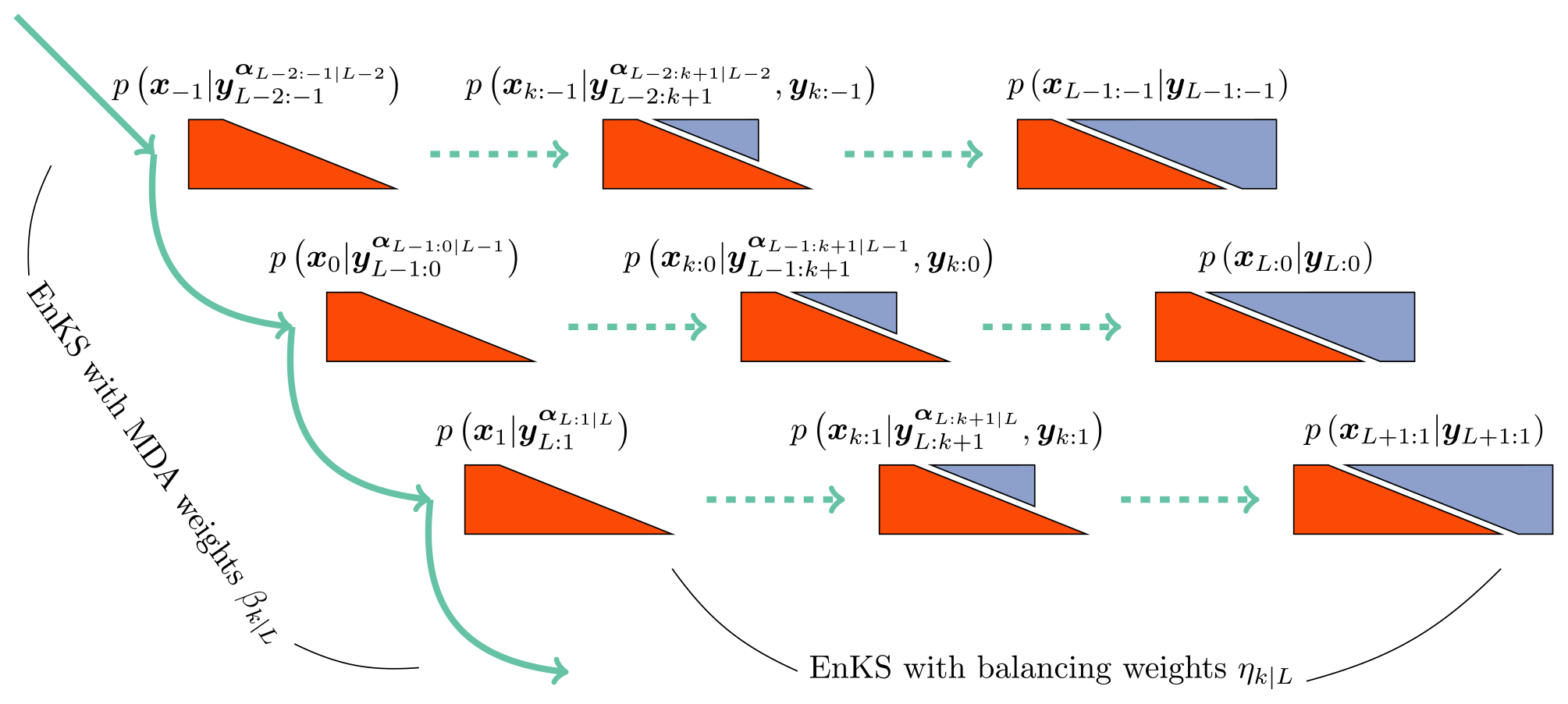
Figure 5 A schematic of the two stages of the SIEnKS MDA cycle. The DAW of the SIEnKS moves forward in time, from top to bottom, where the EnKS stage using MDA weights pushes the MDA conditional density, on the far left, forward in time. The middle layer represents the indexing of the stationary DAW, while the top layer represents a DAW one cycle back in time, and the bottom layer represents a DAW one cycle forward in time. The balancing density is sampled sequentially and recursively with an EnKS stage, using the balancing weights and moving from left to right in each cycle. For the current DAW, the middle balancing density has fully assimilated observations y_k:0 and has partially assimilated observations ${\mathit{y}}_{L:k+\mathrm{1}}^{{\mathit{\alpha }}_{L-\mathrm{1}:k+\mathrm{1}|L-\mathrm{1}}}$. The EnKS stage with balancing weights completes when sampling the joint posterior, and the EnKS stage with MDA weights begins again.

The MDA algorithm is generalized to shift windows of S>1 with the number of ensemble forecasts remaining invariant at 2L when using blocks of uniform MDA weights in the DAW. Assume that L=SQ for some positive integer Q, so that we partition y_L:1 into Q total blocks of observations each of length S. In this case, the perfect linear Gaussian model consistency constraint is revised as follows:

$$\begin{array}{}\text{(97)}& {\mathit{\beta }}_{k|L}={\stackrel{\mathrm{̃}}{\mathit{\beta }}}_{i|L}\text{for }i:=\left[{\displaystyle \frac{k}{S}}\right],\text{with }\sum _{j=\mathrm{1}}^Q{\stackrel{\mathrm{̃}}{\mathit{\beta }}}_{j|L}=\mathrm{1},\end{array}$$

where the above brackets represent rounding up to the nearest integer. This ensures, again, that the weights corresponding to the Q total times to which y_k is assimilated sum to one. With this weighting scheme, the equivalence between the balancing and MDA stages' first EnKS filter analysis extends to the first S total EnKS filter analyses, and therefore, ${\mathbf{E}}_S^{\mathrm{mda}}\equiv {\mathbf{E}}_S^{\mathrm{bal}}$ initializes the MDA stage. Memory usage is further reduced by only performing the retrospective conditioning in the balancing stage on the states ${\mathbf{E}}_{S:\mathrm{0}}^{\mathrm{bal}}$. This samples the density $p\left({\mathit{x}}_{S:\mathrm{0}}\right|{\mathit{y}}_{L:\mathrm{0}})$ in the final cycle before the estimates for these states are discarded from all subsequent DAWs. MDA variants of the SIEnKS and the (Lin-)IEnKS are presented in Algorithms A12 and A13.

The primary difference between the SIEnKS and IEnKS MDA schemes lies in the 3D filter balancing analysis versus the global 4D balancing analysis. The IEnKS MDA scheme is not always robust in its 4D balancing estimation because the MDA conditional prior estimate that initializes the scheme may lie far away from the solution for the balanced, joint posterior. As a consequence, the optimization may require many iterations of the balancing stage. On the other hand, the sequential SIEnKS MDA approach uses the partially unassimilated observations in the DAW directly as a boundary condition to the interpolation of the joint posterior estimate over the DAW with the sequential EnKS filter cycle. For long DAWs, this means that the SIEnKS controls error growth in the ensemble simulation that accumulates over the long free forecast in the 4D analysis of the IEnKS.

Note how the cost of assimilation scales differently between the SIEnKS and the IEnKS when performing MDA. Both the IEnKS and the SIEnKS use the same weights η_k|L and β_k|L for their balancing and MDA stages. However, each stage of the IEnKS separately performs an iterative optimization of the 4D cost function. While each iteration therein requires only a single square root inverse calculation of the cost function Hessian, the iterative solution requires at least 2L total ensemble simulations in order to optimize and interpolate the estimates over the DAW. An efficient version of the scheme can be performed as such by using the same free ensemble simulation initialized, as in Eq. (89), in order to assimilate each of the observation sequences ${\mathit{y}}_{L:\mathrm{1}}^{{\mathit{\eta }}_{L:\mathrm{1}|L}}$ and ${\mathit{y}}_{L:\mathrm{1}}^{{\mathit{\beta }}_{L:\mathrm{1}|L}}$. However, the IEnKS additionally requires S total ensemble simulations in order to shift the DAW thereafter. This differs from the SIEnKS, which requires fixed 2L ensemble simulations over the DAW. However, the computational barrier to the SIEnKS MDA scheme lies in the fact that it requires 2L−S square root inverse calculations, corresponding to each unique filter cost function solution over the two stages; in the case that MDA is combined with, e.g., the ensemble transform in the MLEF, this further grows to the sum of the number of iterations ${\sum }_{j=\mathrm{1}}^{\mathrm{2}L-S}{i}_j$, where i_j iterations are used in the jth optimization of a filter cost function. However, when the cost of an ensemble simulation is sufficiently greater than the cost of the square root inverse in the ensemble dimension, the SIEnKS MDA scheme can substantially reduce the leading-order computational cost of the ensemble variational smoothing with MDA, especially when S>1.

4.4 Asynchronous data assimilation

In real-time prediction, fixed-lag smoothers with shifts in S>1 are computationally more efficient in terms of reducing the number of smoother cycles necessary to traverse a time series of observations with sequential DAWs – versus a shift of one, the number of cycles necessary is reduced by the factor of S. A barrier to using the SIEnKS with S>1 lies in the fact that the sequential filter analysis of the EnKS does not in and of itself provide a means to asynchronously assimilate observations. However, the SIEnKS differs from the EnKS in numerically simulating lagged states in the DAW. When one interpolates the posterior estimate with the dynamical model over lagged states, one can easily revise the algorithm to assimilate any newly available data corresponding to a time within the past simulation window, though the weights in MDA need to be adjusted accordingly. There are many ways in which one may even design methods of excluding observations and reintroducing them in a later DAW with a shift S>1. In the current work, the SIEnKS assimilates all observations synchronously, even with S>1. A systematic investigation of algorithms that would optimize this asynchronous assimilation in single-iteration smoothers goes beyond the scope of the current work. However, this key difference between the EnKS and the SIEnKS will be considered later.

5 Numerical benchmarks

5.1 Algorithm cost analysis

Fix the ensemble size N_e in the following, and let us suppose that the cost of the nonlinear ensemble simulation is fixed in Δt, equal to C_ℳ floating-point operations (flops). In order to compute the ensemble transform in any of the methods, we assume that the inversion of the approximate Hessian ${\stackrel{\mathrm{̃}}{\mathbf{\Xi }}}_{\stackrel{\mathrm{̃}}{\mathcal{J}}}$, and its square root, is performed with an SVD-based approach with the cost of the order of $\mathcal{O}\left(N_{\mathrm{e}}^{\mathrm{3}}\right)$ flops. This assures stability and efficiency in the sense that the computation of all of $\mathbf{T}={\stackrel{\mathrm{̃}}{\mathbf{\Xi }}}_{\stackrel{\mathrm{̃}}{\mathcal{J}}}^{-\frac{\mathrm{1}}{\mathrm{2}}}$, ${\mathbf{T}}^{-\mathrm{1}}={\stackrel{\mathrm{̃}}{\mathbf{\Xi }}}_{\stackrel{\mathrm{̃}}{\mathcal{J}}}^{\frac{\mathrm{1}}{\mathrm{2}}}$ and ${\stackrel{\mathrm{̃}}{\mathbf{\Xi }}}_{\stackrel{\mathrm{̃}}{\mathcal{J}}}^{-\mathrm{1}}$ combined is dominated by the cost of the SVD of the symmetric, which is N_e×N_e matrix ${\stackrel{\mathrm{̃}}{\mathbf{\Xi }}}_{\stackrel{\mathrm{̃}}{\mathcal{J}}}$. If a method is iterative, we denote the number of iterations used in the scheme with i_j, where the sub-index j distinguishes distinct iterative optimizations.

A summary of how each of the S/I/EnKS scale in their numerical cost is presented in Tables 1 and 2. This analysis is easily derived based on the pseudo-code in Appendix A and with the discussions in Sect. 4. Table 1 presents schemes that are used in the SDA configuration, while Table 2 presents schemes that are used in the MDA configurations. Note that, while adaptive inflation in the finite size formalism can be used heuristically to estimate a power of the joint posterior, this has not been found to be fully compatible with MDA (Bocquet and Sakov, 2014), and this combination of techniques is not considered here.

Table 1 Order of the SDA cycle flops for lag=L, shift=S, tuned inflation (TI), or adaptive inflation (AI)/nonlinear observation operator (NO).

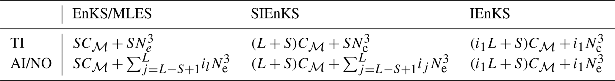
For realistic geophysical models, note that the maximal ensemble size N_e is typically of the order of 𝒪(10²), while the state dimension N_x can be of the order of 𝒪(10⁹) (Carrassi et al., 2018); therefore, the cost of all algorithms is reduced to terms of $C_{\mathcal{M}}\gg N_{\mathrm{e}}^{\mathrm{3}}$ at leading-order in target applications. It is easy to see then that the EnKS/MLES has a cost that is of the order of the regular ETKF/MLEF filter cycle, representing the least expensive of the estimation schemes. Consider now, in row one of Table 1, that the i₁ in the IEnKS represents the number of iterations utilized to minimize the 4D cost function. If we set i₁=1, then this represents the cost of the Lin-IEnKS. Particularly, we see that, for S=1 and a linear filter cost function, the Lin-IEnKS has the same cost as the SIEnKS. However, even in the case of a linear filter cost function, when S>1, then the SIEnKS is more expensive than the Lin-IEnKS. Setting i₁ in Table 1 to terminate with a maximum possible value the cost of the IEnKS is bounded at the leading order; yet, we demonstrate shortly how the number of iterations tends to be small in stable filter regimes.

Consider the case when the filter cost function is nonlinear, as when adaptive inflation is used (as defined in Sect. 4.2), or when there is a nonlinear observation operator. Row two of Table 1 shows how the cost of these estimators is differentiated when nonlinearity is introduced – particularly, the cost of the MLES and the SIEnKS requires one SVD calculation for each iteration used to process each new observation. This renders the SIEnKS notably more expensive than the Lin-IEnKS, which uses a single Hessian SVD calculation to process all observations globally. However, for target applications, such as synoptic-scale meteorology, the additional expense of iteratively optimizing filter cost functions with the SIEnKS versus the single iteration of the Lin-IEnKS in the 4D cost function is insignificant.

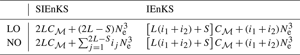
Table 2 describes the cost of the SIEnKS and the IEnKS using MDA when there is a linear observation operator and when there is a nonlinear observation operator. Recall that, at leading-order C_ℳ, the cost of the SIEnKS is invariant in S. This again comes with the caveat that observations are assumed to be assimilated synchronously in this work, while the IEnKS assimilates observations asynchronously by default. Nonetheless, the equivalence between the first S-filter cycles in the balancing stage and the MDA stage in the SIEnKS allows the scheme to fix the leading-order cost at the expense of two passes over the DAW with the ensemble simulation.

Table 2 Order of the MDA cycle flops for lag $=L=Q\times S$, shift =S, tuned inflation, linear observation operator (LO), or nonlinear observation operator (NO).

5.2 Data assimilation benchmark configurations

To demonstrate the performance advantages and limitations of the SIEnKS, we produce statistics of its forecast/filter/smoother root mean square error (RMSE) versus the EnKS/Lin-IEnKS/IEnKS in a variety of DA benchmark configurations. Synthetic data are generated in a twin experiment setting, with a simulated truth twin generating the observation process. Define the truth twin realization at time t_k as ${\mathit{x}}_k^{\mathrm{t}}$; we define the ensemble RMSE as follows:

$$\begin{array}{}\text{(98)}& {\displaystyle }\mathrm{RMSE}\left({\mathbf{E}}_k^i\right):=\sqrt{\sum _{j=\mathrm{1}}^{N_x}{\displaystyle \frac{{\left({\widehat{x}}_{j,k}^i-x_{j,k}^{\mathrm{t}}\right)}^{\mathrm{2}}}{N_x}}},\end{array}$$

where i refers to an ensemble label $i\in \mathit{\{}\mathrm{fore},\mathrm{filt},\mathrm{smth},\mathrm{bal},\mathrm{mda}\mathit{\}}$, j refers to the state dimension index $j\in \mathit{\{}\mathrm{1},\mathrm{\cdots },N_x\mathit{\}}$, and k refers to time t_k as usual.

A common diagnostic for the accuracy of the linear Gaussian approximation in the DA cycle is verifying that the ensemble RMSE has approximately the same order as the ensemble spread (Whitaker and Loughe, 1998), which is known as the spread–skill relationship; overdispersion and underdispersion of the ensemble both indicate the inadequacy of the approximation. Define the ensemble spread as follows:

$$\begin{array}{}\text{(99)}& {\displaystyle }\mathrm{spread}\left({\mathbf{E}}_k^i\right):=\sqrt{{\displaystyle \frac{\mathrm{1}}{N_{\mathrm{e}}-\mathrm{1}}}\sum _{j=\mathrm{1}}^{N_{\mathrm{e}}}{\displaystyle \frac{{\left({\mathbf{X}}_k^{i,j}\right)}^{\top }\left({\mathbf{X}}_k^{i,j}\right)}{N_x}}},\end{array}$$

where i again refers to an ensemble matrix label, j in this case refers to the ensemble matrix column index, and k again refers to time. The spread is then given by the square root of the mean square deviation of the ensemble from its mean. Performance of these estimators will be assessed in terms of having low RMSE scores with the spread close to the value of the RMSE. Estimators are said to be divergent when either the filter or smoother RMSE is greater than the standard deviation of the observation errors, indicating that initializing a forecast with noisy observations is preferable to the posterior estimate. The perfect hidden Markov model in this study is defined by the single-layer form of the Lorenz 96 equations (Lorenz, 1996). The state dimension is fixed at N_x=40, with the components of the vector x given by the variables x_j with periodic boundary conditions, x₀=x₄₀, $x_{-\mathrm{1}}=x_{\mathrm{39}}$, and x₄₁=x₁. The time derivatives $\frac{\mathrm{d}\mathit{x}}{\mathrm{d}t}:=\mathit{f}\left(\mathit{x}\right)$, also known as the model tendencies, are given for each state component $j\in \mathit{\{}\mathrm{1},\mathrm{\cdots },\mathrm{40}\mathit{\}}$ by the following:

$$\begin{array}{}\text{(100)}& {\displaystyle }{f}_j\left(\mathit{x}\right){\displaystyle }=-x_{j-\mathrm{2}}{x}_{j-\mathrm{1}}+x_{j-\mathrm{1}}{x}_{j+\mathrm{1}}-x_j+F.\end{array}$$

Each state variable heuristically represents the atmospheric temperature at one of the 40 longitudinal sectors discretizing a latitudinal circle of the Earth. The Lorenz 96 equations are not a physics-based model, but they mimic the fundamental features of geophysical fluid dynamics, including conservative convection, external forcing, and linear dissipation of energy (Lorenz and Emanuel, 1998). The term F is the forcing parameter that injects energy into the model, and the quadratic terms correspond to energy-preserving convection, while the linear term −x_j corresponds to dissipation. With F≥8, the system exhibits chaotic, dissipative dynamics; we fix F=8 in the following simulations, with the corresponding number of unstable and neutral Lyapunov exponents being equal to N₀=14.

For a fixed Δt, the dynamical model ℳ_k is defined by the flow map generated by the dynamical system in Eq. (100). Both the truth twin simulation, generating the observation process, and ensemble simulation, used to sample the appropriate conditional density, are performed with a standard four-stage Runge–Kutta scheme with the step size h=0.01. This high-precision simulation is used for generating a ground truth for these methods, validating the Julia package DataAssimilationBenchmarks.jl (Grudzien et al., 2021) and testing its scalability; however, in general, h=0.05 should be of sufficient accuracy and is recommended for future use. The nonlinearity of the forecast error evolution is controlled by the length of the forecast window, Δt. A forecast length Δt=0.05 corresponds to a 6 h atmospheric forecast, while for Δt>0.05, the level of nonlinearity in the ensemble simulation can be considered to be greater than that which is typical of synoptic-scale meteorology.

Localization, hybridization, and other standard forms of ensemble-based gain augmentation are not considered in this work for the sake of simplicity. Therefore, in order to control the growth of forecast errors under weakly nonlinear evolution, the rank of the ensemble-based gain must be equal to or greater than the number of unstable and neutral Lyapunov exponents N₀=14, corresponding to N_e≥15 (see Grudzien et al., 2018, and references therein). In the following experiments, we range the ensemble size as $N_{\mathrm{e}}\in \mathit{\{}\mathrm{15}+\mathrm{2}i{\mathit{\}}}_{i=\mathrm{0}}^{\mathrm{13}}$, from the minimal rank needed without gain augmentation to a full-rank ensemble-based gain. When the number of experimental parameters expands, we restrict to the case where N_e=21 for an ensemble-based gain of actual rank 20, making a reduced-rank approximation of the covariance in analogy to DA in geophysical models.

Observations are full dimensional, such that $N_y=N_x=\mathrm{40}$, and observation errors are distributed according to the Gaussian density $n\left(\mathit{z}|\mathbf{0},{\mathbf{I}}_{N_y}\right)$, i.e., with mean zero, uncorrelated across state indices and with homogeneous variances equal to one. When the observation map is linear, it is defined as ${\mathbf{H}}_k:={\mathbf{I}}_{N_x}$; when the observation map is taken to be nonlinear, define the following:

$$\begin{array}{}\text{(101)}& {\displaystyle }\mathcal{H}\left(\mathit{x}\right):={\displaystyle \frac{\mathit{x}}{\mathrm{2}}}\circ \left\{\mathbf{1}+{\left({\displaystyle \frac{\mathit{x}}{\mathrm{10}}}\right)}^{\mathit{\gamma }-\mathrm{1}}\right\},\end{array}$$

where ∘ above refers to the Schur product. This observation operator is drawn from Sect. 6.7.2.2 of Asch et al. (2016), where the parameter γ controls the nonlinearity of the map. In particular, for γ=1, this corresponds to the linear observation operator H_k, while γ>1 increases the nonlinearity of the map. When we vary the nonlinearity of the observation operator, we take $\mathit{\gamma }\in \mathit{\{}i{\mathit{\}}}_{i=\mathrm{1}}^{\mathrm{11}}$ corresponding to 10 different nonlinear settings and the linear setting for reference.

When tuned inflation is used to regularize the smoothers, as in Algorithm A4, we take a discretization range of $\mathit{\lambda }\in \mathit{\{}\mathrm{1.0}+\mathrm{0.01}i{\mathit{\}}}_{i=\mathrm{0}}^{\mathrm{10}}$, corresponding to the usual Kalman update with λ=1.0 and to up to 10 % inflation of the empirical variances with λ=1.1. Using tuned inflation, estimator performance is selected for the minimum average forecast RMSE over the experiment for all choices of λ, unless this is explicitly stated otherwise. When adaptive inflation is used, no additional tuned inflation is utilized. Simulations using the finite size formalism will be denoted with -N, following the convention of the EnKF-N. Multiple data assimilation will always be performed with uniform weights as ${\mathit{\beta }}_{k|L}:=\frac{\mathrm{1}}{L}$ for all estimators.

For the IEnKS, we limit the maximum number of iterations per stage at i_j=10 for $j=\mathrm{1},\mathrm{2}$. Therefore the IEnKS can take a maximum of $i_{\mathrm{1}}+i_{\mathrm{2}}=\mathrm{20}$ iterations in the MDA configuration to complete a cycle. Iteratively optimizing the filter cost function in the MLES(-N)/SIEnKS(-N), the maximum number of iterations is capped at i_j=40 per analysis. The tolerance for the stopping condition in the filter cost functions is set to 10⁻⁴, while the tolerance for the 4D estimates is set to 10⁻³. However, the scores of the algorithms are, to a large extent, insensitive to these particular hyperparameters.

In order to capture the asymptotically stationary statistics of the filter/forecast/smoother processes, we take a long time-average of the RMSE and spread over the time indices k. The long experiment average ensures that, for an ergodic dynamical system, we average over the spatial variation in the attractor, and we account for variations in the observation noise realizations that may affect the estimator performance. So that the truth twin simulates observations on the attractor, it is simulated for an initial spinup of 5×10³ analysis times before observations are given. Let the time be given as t₀ after this initial spinup. Observations are generated identically for all estimators using the same Gaussian error realizations at a given time to perturb the observation map of the truth twin. At time t₀, the ensemble is initialized identically for all estimators (depending on the ensemble size) with the same iid sample drawn from the multivariate Gaussian with mean at the truth twin ${\mathit{x}}_{\mathrm{0}}^{\mathrm{t}}$ and covariance equal to the identity ${\mathbf{I}}_{N_x}$. All estimation schemes are subsequently run over observation times indexed as $\mathit{\{}{t}_k{\mathit{\}}}_{k=\mathrm{1}}^{\mathrm{2.5}\times {\mathrm{10}}^{\mathrm{4}}}$. As the initial warmup of the estimators' statistics from this cold start tends to differ from the asymptotically stationary statistics, we discard the forecast/filter/smoother RMSE and spread corresponding to the observations times $\mathit{\{}{t}_k{\mathit{\}}}_{k=\mathrm{1}}^{\mathrm{5}\times {\mathrm{10}}^{\mathrm{3}}}$, taking the time average of these statistics for the remaining 2×10⁴ analysis time indices. Particularly, this configuration is sufficient to represent estimator divergence which may have a delayed onset.

Forecast statistics are computed for each estimator whenever the ensemble simulates a time index t_k for the first time, before y_k has been assimilated into the estimate. Filter statistics are computed in the first analysis at which the observation y_k is assimilated into the simulation. For the (Lin-)IEnKS, with S>1, this filter estimate includes the information from all observations ${\mathit{y}}_{L:L-S+\mathrm{2}}$ when making a filter estimate for the state at $t_{L-S+\mathrm{1}}$. Smoother statistics are computed for the time indices $t_{\mathrm{0}},t_{\mathrm{1}},\mathrm{\cdots },t_{S-\mathrm{1}}$ in each cycle, corresponding to the final analysis for these states before they are discarded from subsequent DAWs. Empty white blocks in heat plots correspond to Inf (non-finite) values in the simulation data. Missing data occur due to numerical overflow when attempting to invert a close-to-singular cost function Hessian ${\stackrel{\mathrm{̃}}{\mathbf{\Xi }}}_{\stackrel{\mathrm{̃}}{\mathcal{J}}}$, which is a consequence of the collapse of the ensemble spread. When an estimator suffers this catastrophic filter divergence, the experiment output is replaced with Inf values to indicate the failure. Other benchmarks for the EnKS/Lin-IEnKS/IEnKS in the Lorenz 96 model above can be found in, e.g., Bocquet and Sakov (2014), Asch et al. (2016), and Raanes et al. (2018), which are corroborated here with similar but slightly different configurations.

5.3 Weakly nonlinear forecast error dynamics – linear observations

We fix Δt=0.05 in this section, set S=1, and use the linear observation operator in order to demonstrate the baseline performance of the estimators in a simple setting. On the other hand, we vary the lag length, the ensemble size, and the use of tuned/adaptive inflation or MDA. The lag in this section is varied on a discretization of $L\in \mathit{\{}\mathrm{1}+\mathrm{3}i{\mathit{\}}}_{i=\mathrm{0}}^{\mathrm{30}}$. As a first reference simulation, consider the simple case where all schemes use tuned covariance inflation, so that the SIEnKS and the Lin-IEnKS here are formally equivalent. Likewise, with S=1, there is no distinction between asynchronous or synchronous DA. Figure 6 makes a heat plot of the forecast/filter/smoother RMSE and spread as the lag length L is varied along with the ensemble size N_e.

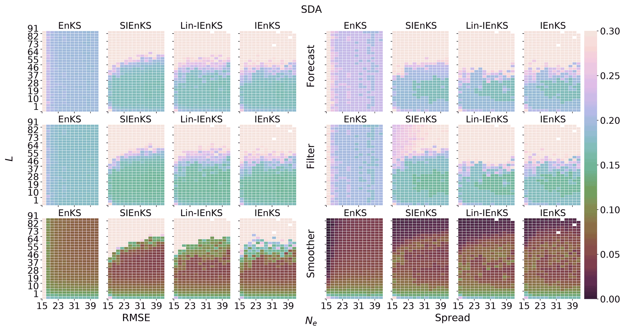
Figure 6 The lag length L is shown on the vertical axis, and the ensemble size N_e is shown on the horizontal axis. SDA, tuned inflation, shift S=1, linear observations, and Δt=0.05 are also indicated.

Figure 7 Cross section of Fig. 6 at the ensemble size N_e=21.

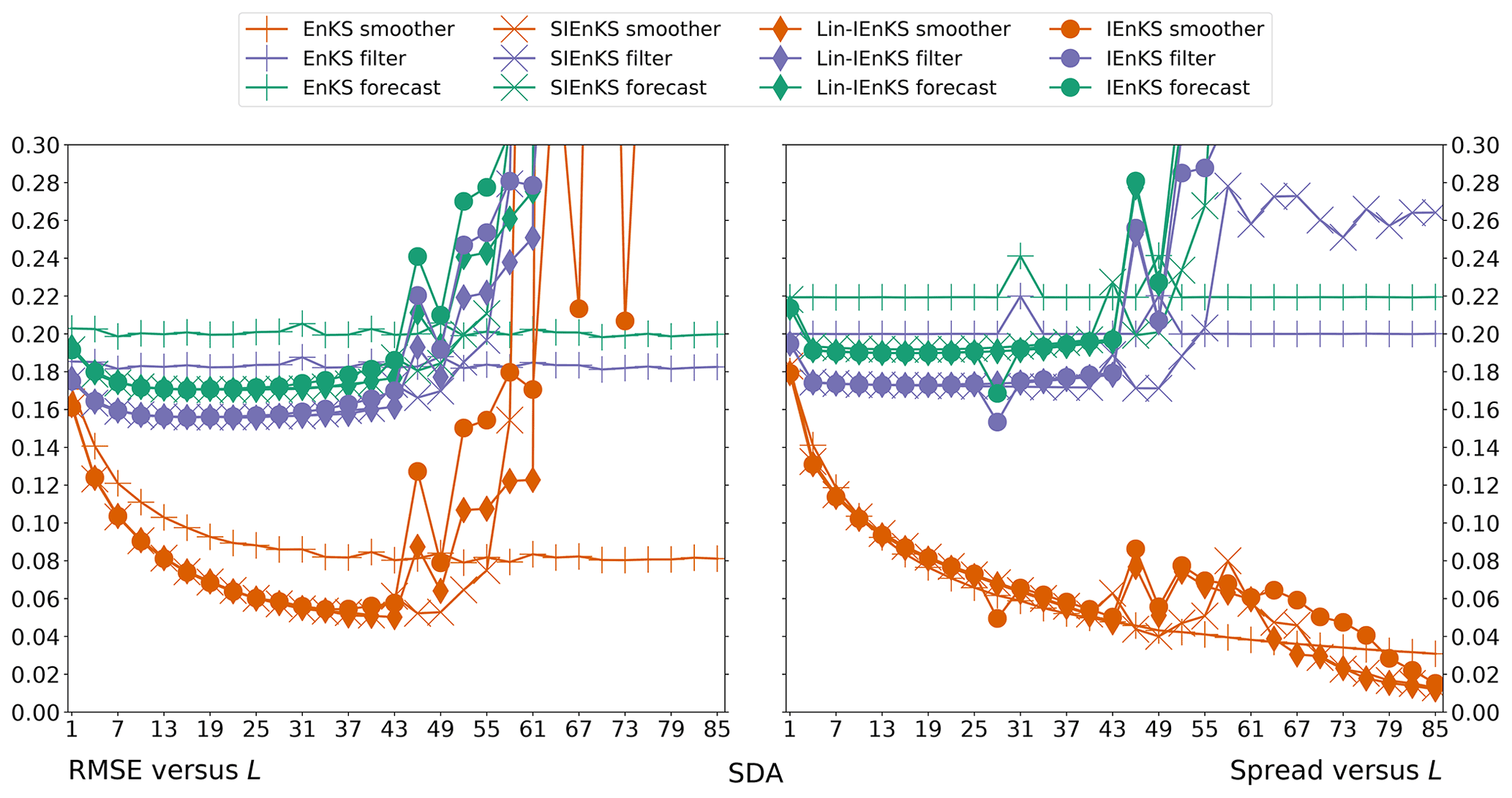
It is easy to see the difference in the performance between the EnKS and the iterative S/Lin-/IEnKS schemes. Particularly, the forecast and filter RMSE does not change with respect to the lag length in the EnKS, as these statistics are generated independently of the lag with a standard ETKF filter cycle. However, the smoother performance of the EnKS does improve with longer lags, without sacrificing stability over a long lag as in the iterative schemes. In particular, all of the iterative schemes use the dynamical model to interpolate the posterior estimate over the DAW. For sufficiently large L, this becomes unstable due to the small simulation errors that are amplified by the chaotic dynamics. The scale of the color map is capped at 0.30, as a more accurate forecast/filter performance can be attained in this setting with the ETKF alone, as demonstrated by the EnKS.

On the other hand, the iterative estimate of the posterior, as in the S/Lin-/IEnKS in this weakly nonlinear setting, shows a dramatic improvement in the predictive and analysis accuracy for a tuned lag length. Unlike the standard ETKF observation/analysis/forecast cycle, these iterative smoothers are able to control the error growth in the neutral Lyapunov subspace corresponding to the N₀=14th Lyapunov exponent. With the ensemble size N_e=15 corresponding to a rank 14 ensemble-based gain, the iterative smoothers maintain stable prediction and posterior estimates over a wide range of lags while the EnKS diverges for all lag settings. We notice that the stability regions of the S/Lin-/IEnKS are otherwise largely the same in this simple benchmark configuration, though the IEnKS has a slightly longer stability over long lags with low sample sizes.

In order to illustrate the difference in accuracy between the iterative schemes and the non-iterative EnKS, Fig. 7 plots a cross section of Fig. 6 for N_e=21. The iterative schemes have almost identical performance until approximately a lag of L≈37, at which point all schemes become increasingly unstable. The differences shown between the iterative schemes here are insignificant and may vary between different implementations of these algorithms or pseudo-random seeds. We note that all estimators are also slightly overdispersive due to selecting a tuned inflation value based on the minimum forecast RMSE rather than balancing the RMSE and spread simultaneously. Nonetheless, we clearly demonstrate how all iterative estimators reduce the prediction and analysis error over the noniterative EnKS approach. Tuning the lag L, the forecast error for the iterative schemes is actually lower than the filter error in the EnKS.

Figure 8 The lag length L is shown on the vertical axis, and the ensemble size N_e is shown on the horizontal axis. SDA, adaptive inflation, shift S=1, linear observations, and Δt=0.05 are also indicated.

Figure 9 Cross section of Fig. 8 at the ensemble size N_e=21.

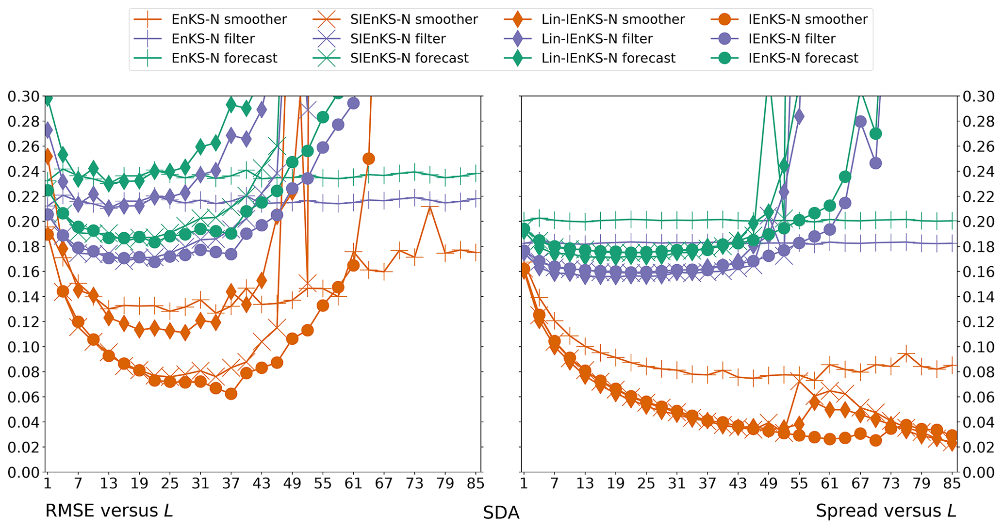
Consider the case where the filter cost function is nonlinear due to the adaptive inflation scheme. Figure 8 makes the same heat plot as in Fig. 6 but where the finite size formalism is used instead of tuned inflation. All schemes tend to have slightly weaker performance in this setting, except for the IEnKS-N in the low-ensemble-size regime. The design of the adaptive inflation scheme is to account for sample error due to the low ensemble size and nonlinearity in the forecast error dynamics, which is typical of mid-range forecasts. The efficacy of the design is illustrated, as the scheme is most effective when the low ensemble size and nonlinear forecast error dynamics conditions are present. Note that the Lin-IEnKS-N uses a single iteration of the extended 4D cost function, optimizing both the weights for the initial condition and the hyperparameter simultaneously. On the other hand, while the SIEnKS-N makes a single iteration of the ensemble simulation over the DAW, it iteratively optimizes the adaptive inflation hyperparameter in the filter cost function. This allows the SIEnKS-N to make substantial improvements over the Lin-IEnKS-N in terms of the stability region while remaining at the same leading-order cost.

Figure 9 plots a cross section of Fig. 8 at N_e=21 in order to further demonstrate the improved accuracy of the forecast/filter/smoother statistics of the SIEnKS-N versus the Lin-IEnKS-N. For a tuned lag L, the Lin-IEnKS-N fails to achieve distinctly better forecast and filter accuracy than the EnKS-N. While the smoother RMSE for the Lin-IEnKS-N does make an improvement over the EnKS-N, this improvement is not comparable to the smoother accuracy of the SIEnKS-N, which has the same leading-order cost. The performance of the SIEnKS-N is almost indistinguishable from the 4D IEnKS-N up to a lag of L≈25. At this point, the stability of the SIEnKS-N begins to suffer, while, on the other hand, the IEnKS-N is able to improve smoother RMSE for slightly longer lags. Nonetheless, both the SIEnKS-N and the IEnKS-N become increasingly underdispersive for lags L≥25, demonstrating the systematic underestimation of the estimator's uncertainty that leads to divergence for sufficiently large L.

We now demonstrate how MDA relaxes the nonlinearity of the MAP estimation and the interpolation of the posterior estimate over the DAW. Recall that MDA is handled differently in the SIEnKS from the 4D schemes because the 4D approach interpolates the DAW with the balancing estimate from a free forecast, while the SIEnKS interpolates the posterior estimate via a sequence of filter analyses steps using the balancing weights. Recall that, for target applications, the SIEnKS is the least expensive MDA estimator, requiring only 2L ensemble simulations in this configuration, while the (Lin-)IEnKS uses at least 2L+1. Figure 10 presents the same experiment configuration as in Figs. 6 and 8 but where MDA is used with tuned inflation. The EnKS does not use MDA, but the results from Fig. 6 are presented here for reference.

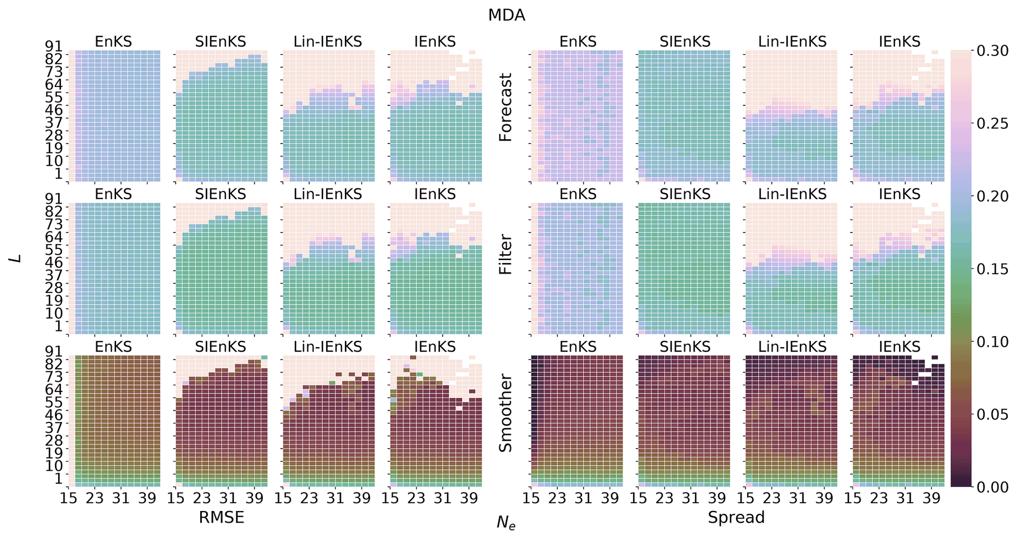
Figure 10 The lag length L is shown on the vertical axis, and the ensemble size N_e is shown on the horizontal axis. MDA, tuned inflation, shift S=1, linear observations, and Δt=0.05 are indicated. The EnKS SDA results are presented here for reference.

Figure 11 Cross section of Fig. 10 at the ensemble size N_e=21.

It is easy to see that MDA improves all of the iterative smoothing schemes in Fig. 10, with greatly expanded stability regions from Fig. 6. Moreover, a key new pattern emerges that differentiates the traditional 4D MDA approach and the new MDA scheme in the SIEnKS. In particular, while the stability regions for the SIEnKS/(Lin-)IEnKS are similar for their smoother statistics in this configuration, the forecast/filter statistics are strongly differentiated. Unlike the free forecast solution used to interpolate the posterior estimate over the DAW in the 4D approach, the filter step within the SIEnKS MDA controls the simulation errors that accumulate when L is large.

In order to examine the effect more precisely, consider the cross section of Fig. 10 for N_e=21 presented in Fig. 11. Notice that all iterative MDA estimators have almost indistinguishable performance until lag L≈31. From this point, although the smoother accuracy increases with longer lags for the (Lin-)IEnKS, this comes at a sacrifice in the forecast/filter accuracy. Particularly, for lags L≥31, the forecast/filter accuracy of the (Lin-)IEnKS begins to degrade; at a lag of L≈61, the IEnKS performs worse than the EnKS, while the Lin-IEnKS has diverged. This is in stark contrast to the SIEnKS because not only does the forecast/filter accuracy remain stable for lags L≥40, but each of these also improve along with the smoother accuracy until a lag L≈61. Furthermore, the spread of the SIEnKS indicates that the SIEnKS MDA and perfect linear Gaussian approximation is well satisfied, with the ensemble dispersion very close to the RMSE within the stability region.

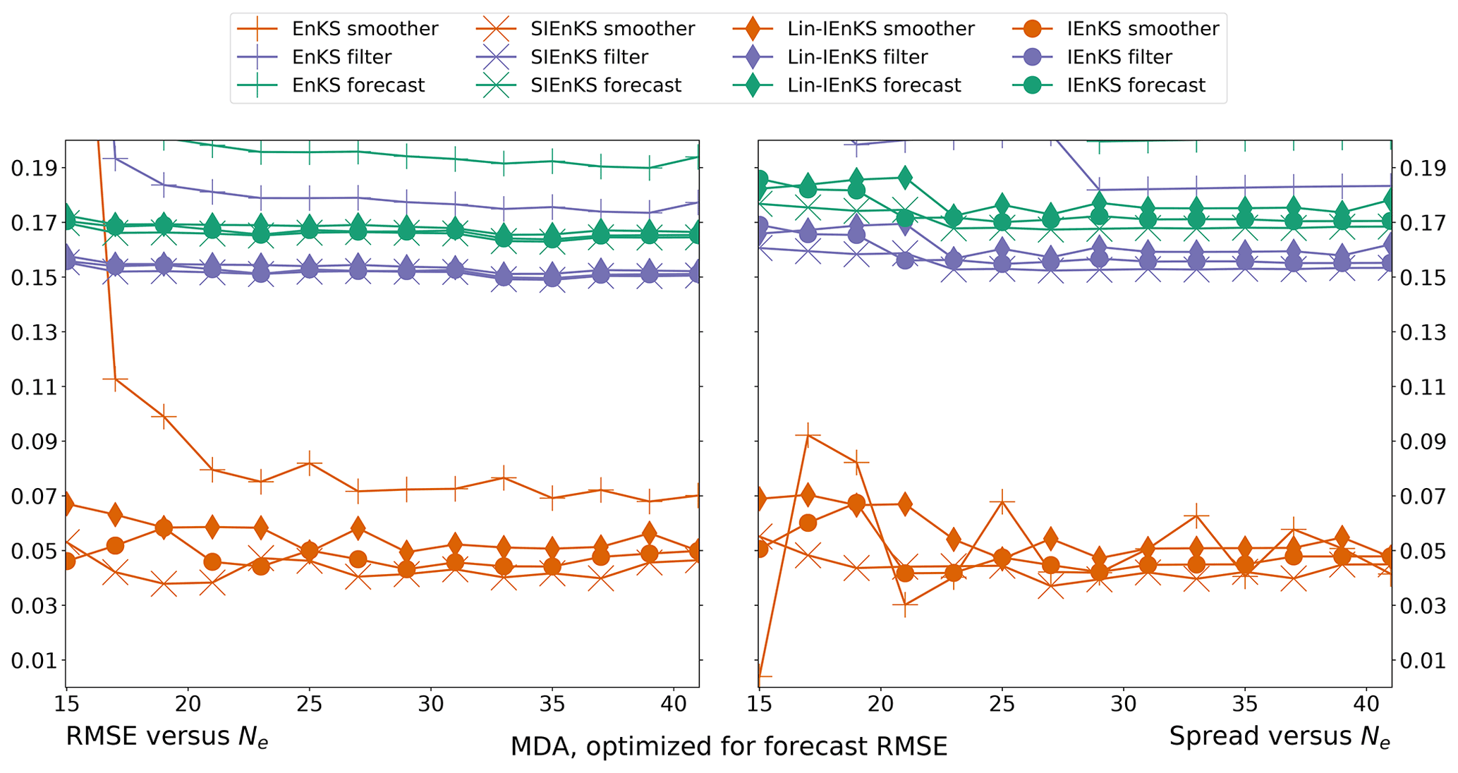
Figure 12 MDA configuration. RMSE and spread versus the ensemble size N_e. Lag and inflation are optimized for a minimum forecast RMSE in Fig. 10.

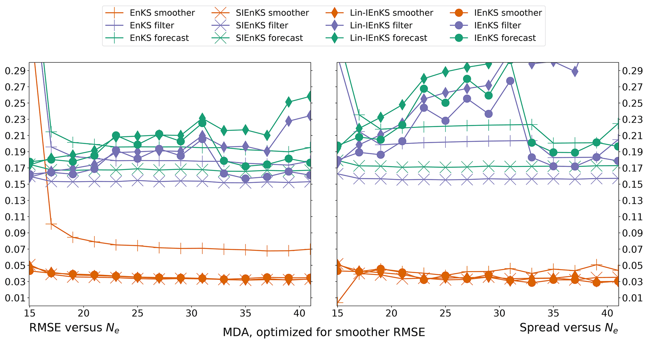
Figure 13 MDA configuration. RMSE and spread versus the ensemble size N_e. Lag and inflation are optimized for a minimum forecast RMSE in Fig. 10.

The SIEnKS thus highlights a performance tradeoff of the 4D MDA schemes that it does not suffer from itself. In particular, suppose that the lag L in Fig. 10 is selected in order to optimize each estimator's accuracy, in terms of RMSE, for each fixed ensemble size N_e. One can optimize the lag L using the forecast RMSE or the smoother RMSE as the criterion. However, Fig. 11 indicates that L may be quite different for the forecast accuracy versus the smoother accuracy in the 4D schemes. Figures 12 and 13 demonstrate this tradeoff precisely, where the former plots the RMSE and spread, with lag and inflation simultaneously optimized for forecast accuracy, and the latter is optimized for smoother accuracy.

Tuning for optimum forecast RMSE, as in Fig. 12, the performance of the SIEnKS/(Lin-)IEnKS for any fixed N_e is indistinguishable with respect to this metric. On the other hand, the SIEnKS strongly outperforms the Lin-IEnKS and even exhibits a slightly better overall stability and accuracy than the IEnKS across the range of ensemble sizes. The difference in performance is more pronounced when tuning for the minimal smoother RMSE in Fig. 13. Again, the three estimators are indistinguishable in their smoother estimates, but the SIEnKS forms high-precision smoother estimates without sacrificing its predictive accuracy while interpolating the solution over long lags.

Figure 14 Iterations per cycle versus lag L on the vertical axis and ensemble size N_e on the horizontal axis. The mean (top panel) and standard deviation (bottom panel) of the iterations used per cycle from simulations, generating Figs. 6, 8, and 10, are presented.

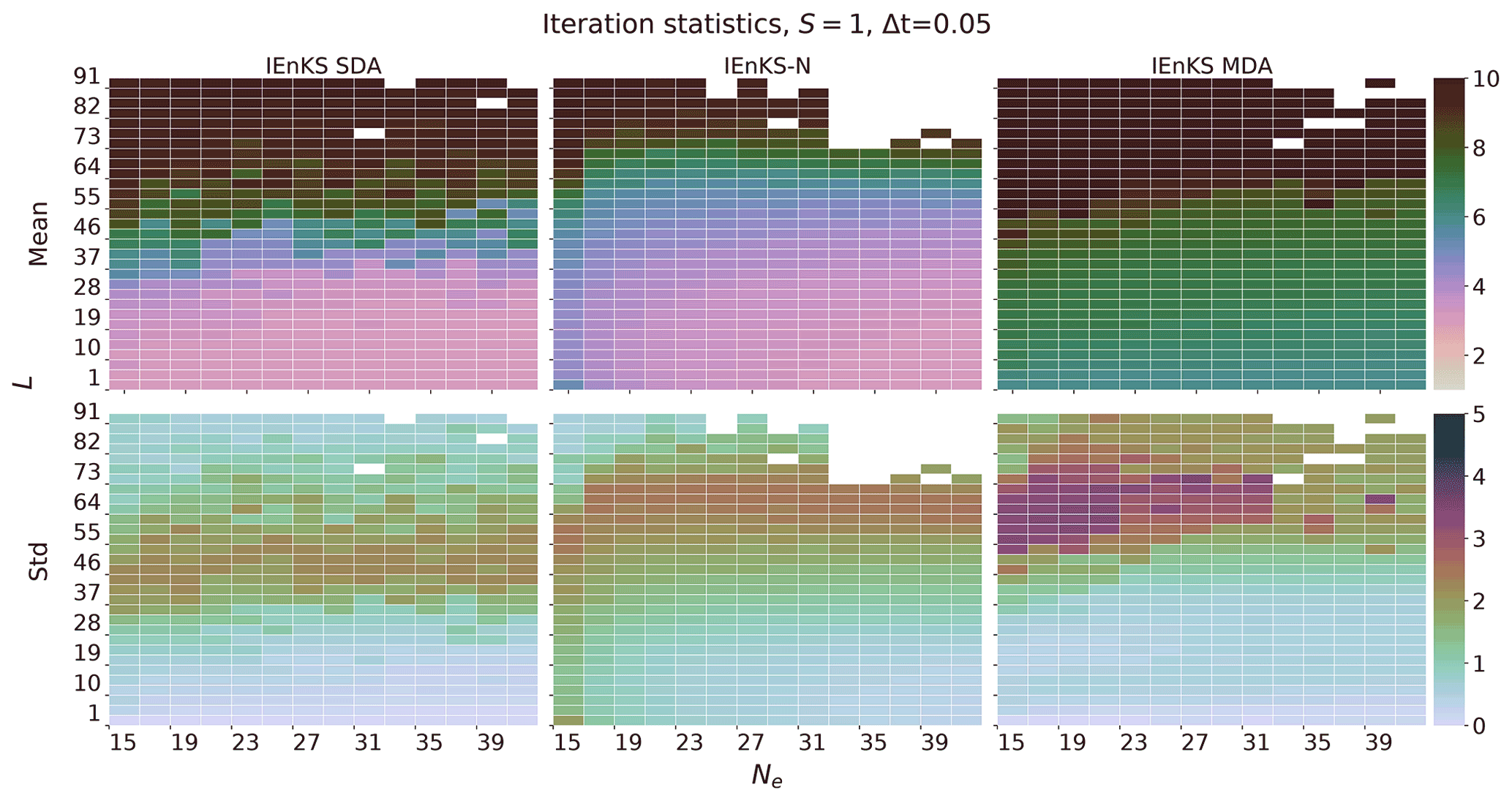
Using MDA or adaptive inflation in DA cycles with weakly nonlinear forecast error dynamics, we demonstrate how the SIEnKS greatly outperforms the Lin-IEnKS with the same, or lower, leading-order cost. The SIEnKS MDA scheme also outperforms the IEnKS MDA scheme with less cost, but the 4D IEnKS-N is able to extract additional accuracy over the SIEnKS-N at the cost of L additional ensemble simulations per iteration. Therefore, it is worth considering the statistics on the number of iterations that the IEnKS uses in each of the above-studied configurations. Figure 14 shows a heat plot for the mean and the standard deviation of the number of iterations used per cycle for each of the IEnKS with SDA, IEnKS-N, and IEnKS with MDA to optimize the 4D cost function. Notice that, in the MDA configuration, the mean and the standard deviation is computed over the two stages of the IEnKS, accounting for both the balancing and MDA 4D cost functions.

Although the number of possible iterations is bounded below by one in the case of SDA and two in the case of MDA, the frequency distribution for the total iterations is not especially skewed within the stability region of the IEnKS. This is evidenced by the small standard deviation, less than or equal to one, that defines the stability region for the scheme. Particularly, the IEnKS typically stabilizes around (i) three iterations in the SDA, with tuned inflation configuration, (ii) three to four iterations in the SDA, with adaptive inflation configuration, and (iii) six to eight iterations in the MDA, with tuned inflation configuration. Therefore, the SIEnKS is shown to make a reduction ranging between (i) 2L, (ii) 2L to 3L, or (iii) 4L to 6L ensemble simulations of the estimator's cycle, on average, versus the IEnKS. While this is unremarkable for the SDA, a tuned inflation configuration where the Lin-IEnKS performs similarly, this demonstrates a strong performance advantage of the SIEnKS in its target application, i.e., in settings with weakly nonlinear forecast error dynamics and other sources of nonlinearity dominating the DA cycle. This an especially profound reduction for the MDA configuration, where the SIEnKS MDA scheme proves to be both the least expensive and the most stable/accurate estimator by far.

5.4 Weakly nonlinear forecast error dynamics – nonlinear observations

A primary motivating application for the SIEnKS is the scenario where the forecast error dynamics is weakly nonlinear but where the observation operator is weakly to strongly nonlinear. There are infinite possible ways for how nonlinearity in the observation operator can be expressed, and the results are expected to strongly depend on the particular operator. In the following, we consider the operator in Eq. (101) for the ability to tune the strength of this effect with the parameter γ. In order to avoid conflating the effect of the nonlinearity in the hyperparameter optimization and the nonlinearity in the observation operator, we suppress adaptive inflation in this section. In this case, SDA and MDA schemes are considered to compare how MDA can be used to temper the effects of local minima in the MAP estimation versus a nonlinear observation operator. We again choose Δt=0.05 to maintain weakly nonlinear forecast error dynamics. We restrict to N_e=21, as we expand the experimental parameters to include γ. The lag is varied as $L\in \mathit{\{}\mathrm{1}+\mathrm{3}i{\mathit{\}}}_{i=\mathrm{0}}^{\mathrm{27}}$.

Figure 15 demonstrates the effect of varying the nonlinearity in the observation operator, where strong differences once again emerge between the retrospective analysis of the MLES and the iterative schemes. The scale of the color map is raised to a maximum of 0.5, as a better performance can be achieved with the MLEF alone, as demonstrated by the MLES. In the MLES, the forecast and analysis error increases almost uniformly in γ, but a very different picture emerges for the iterative smoothers. While the stability regions of the iterative schemes tend to shrink for larger γ, the accuracy of the estimators changes non-monotonically. Moreover, iteratively optimizing the filter cost function in the SIEnKS or the 4D cost function in the IEnKS does not in and of itself guarantee a better performance than the Lin-IEnKS, due to the increasing presence of local minima. Particularly for the SIEnKS and the IEnKS with highly nonlinear observations, this optimization can also become deleterious to the estimator performance, with evidence of instability and catastrophic divergence in these regimes.

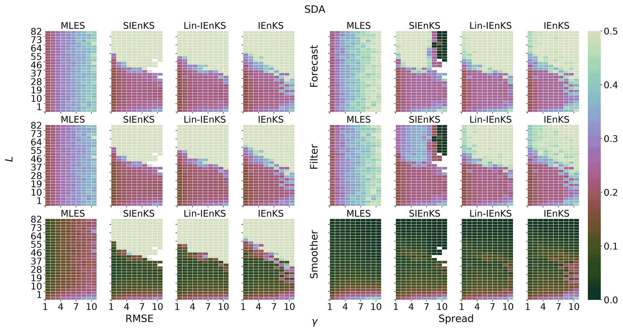
Figure 15 Lag length L on the vertical axis and nonlinearity parameter γ on the horizontal axis. SDA, tuned inflation, shift S=1, N_e=21, and Δt=0.05 are indicated.

In Fig. 16, we repeat the experimental configuration of Fig. 15, with the exception of using the MDA configuration. As seen in Fig. 10, MDA greatly extends the forecast/filter accuracy of the SIEnKS over the 4D schemes. Multiple data assimilation in this context additionally weakens the effect of the assimilation update step, smoothing the cost function contours and expanding the stability regions of all estimators.

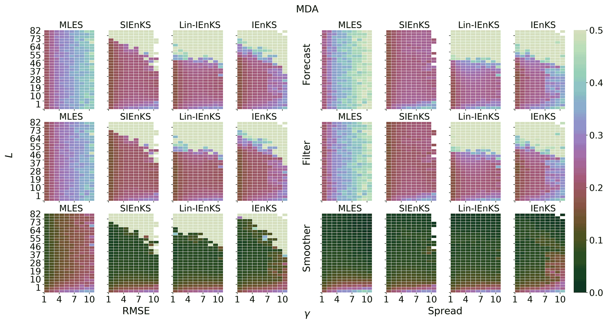
Figure 16 Lag length L is shown on the vertical axis, and the nonlinearity parameter γ is shown on the horizontal axis. MDA, tuned inflation, shift S=1, N_e=21, and Δt=0.05 are indicated. The MLES SDA results are presented here for reference.

Figure 17 presents tuned results from Fig. 16, where the lag and inflation are simultaneously optimized for the minimal forecast RMSE. In this context, we clearly see how the effect of varying γ is non-monotonic on the estimator accuracy for the iterative schemes. However, important differences also emerge in this configuration between the SIEnKS and the (Lin-)IEnKS. While the forecast and filter accuracy of these schemes remains indistinguishable for γ≤7, the smoother RMSE of the SIEnKS is almost uniformly lower than these other schemes for all γ. Interestingly, the degradation of the performance of the IEnKS for highly nonlinear observations, γ≥8, does not extend to either of the Lin-IEnKS or the SIEnKS in the MDA configuration. Whereas the iterative optimization of the 4D cost function becomes susceptible to the effects of the local minima with large γ, the Lin-IEnKS remains stable for the full window of the γ presented here. Moreover, the SIEnKS demonstrates significantly improved smoother accuracy over the Lin-IEnKS while remaining at a lower leading-order cost. This suggests that the sequential MDA scheme of the SIEnKS is better equipped to handle highly nonlinear observation operators than the 4D formalism, which appears to suffer from a greater number of local minima.

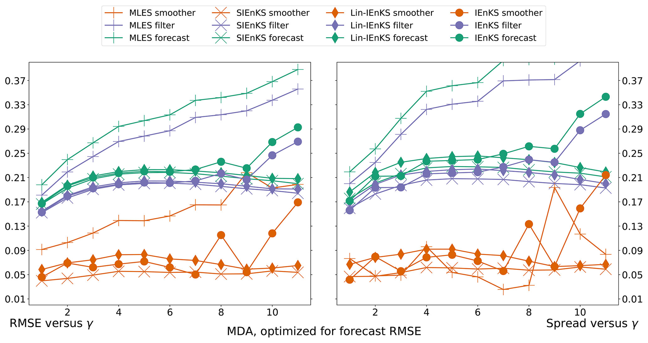
Figure 17 MDA configuration. RMSE and spread versus γ. Lag and inflation are optimized for a minimum forecast RMSE.

5.5 Weakly nonlinear forecast error dynamics – lag versus shift

Even for a linear observation operator and tuned inflation, a shift S>1 distinguishes the performance of each of the studied estimators. In this section, we fix Δt=0.05, corresponding to weakly nonlinear forecast error dynamics, and we vary $L,S\in \mathit{\{}\mathrm{2},\mathrm{4},\mathrm{8},\mathrm{16},\mathrm{32},\mathrm{48},\mathrm{64},\mathrm{80},\mathrm{96}\mathit{\}}$ to demonstrate these differences. For the iterative schemes, we only consider combinations of L divisible by S for compatibility with the MDA schemes. The EnKS is defined for arbitrary S<L, and all such configurations are presented for reference.

Recall the qualification that the EnKS and SIEnKS are designed to assimilate observations sequentially and synchronously in this work, whereas the (Lin-)IEnKS assimilates observations asynchronously by default. When S=1, there is no distinction between asynchronous and synchronous assimilation, but in this section this distinction is borne in mind. Likewise, it is recalled that, for the (Lin-)IEnKS with a shift S>1, filter statistics are computed, including the information from all observations ${\mathit{y}}_{L:L-S+\mathrm{1}}$ when making a filter estimate for states at times $t_{S+\mathrm{1}},\mathrm{\cdots },t_L$. This arises from the asynchronous design of the IEnKS, whereas filter statistics are computed sequentially without future information in the SIEnKS.

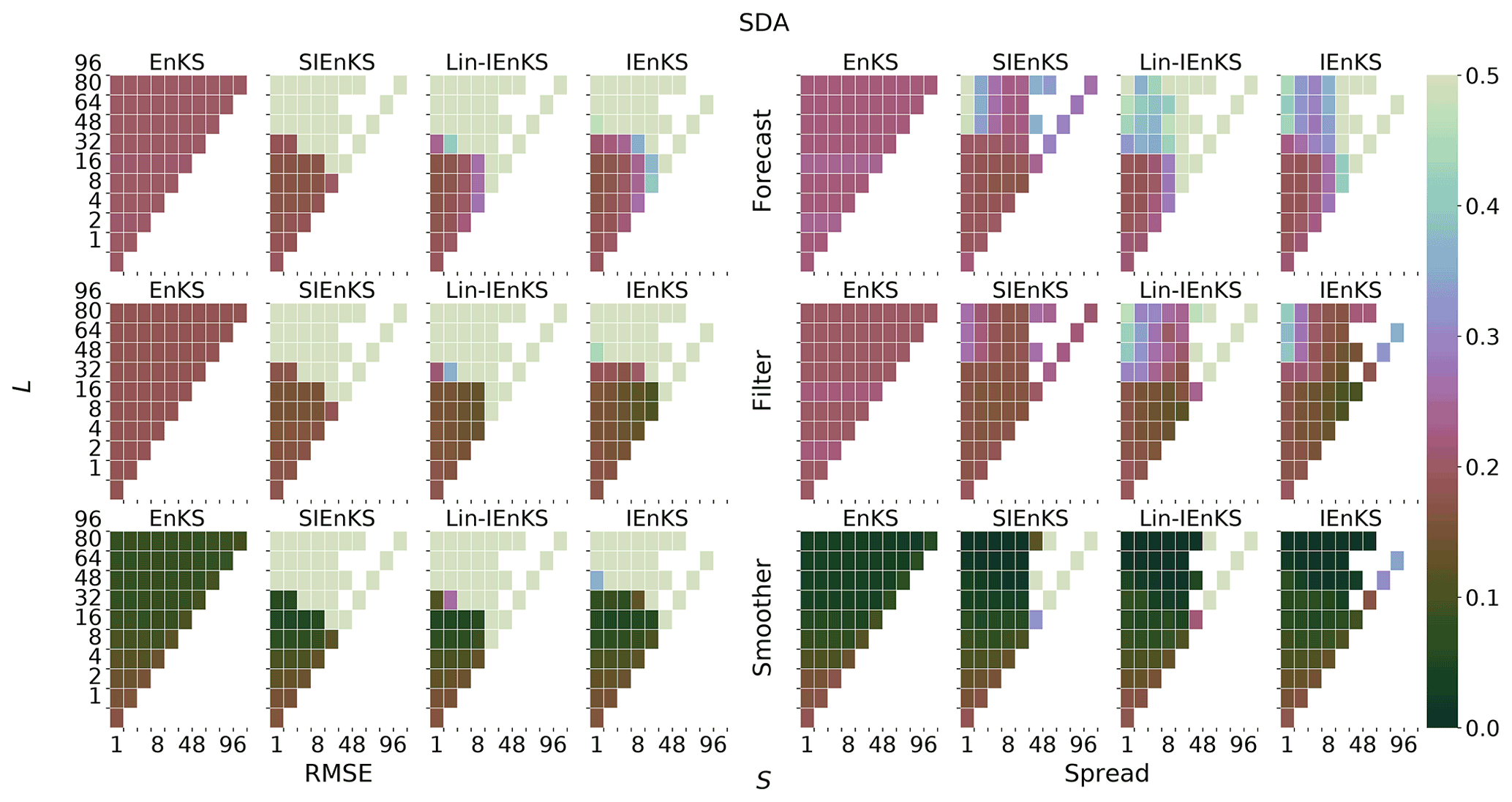
Figure 18 Lag length L on the vertical axis and shift S on the horizontal axis. SDA, tuned inflation, linear observations, ensemble size N_e=21, and Δt=0.05 are indicated.

Figure 18 presents the heat plot of RMSE and spread for each estimator in the SDA configuration. We note that the EnKS for a fixed L has a performance that is largely invariant with respect to changes in S, except for the special case where S=L. In this case, the non-overlapping DAWs impose that posterior estimates are constructed with fewer observations conditioning the final estimate than in overlapping DAWs. Otherwise, the stability regions of the iterative schemes are largely the same, with the SIEnKS only achieving a slight improvement over the Lin-IEnKS and the IEnKS only slightly improving on the SIEnKS.

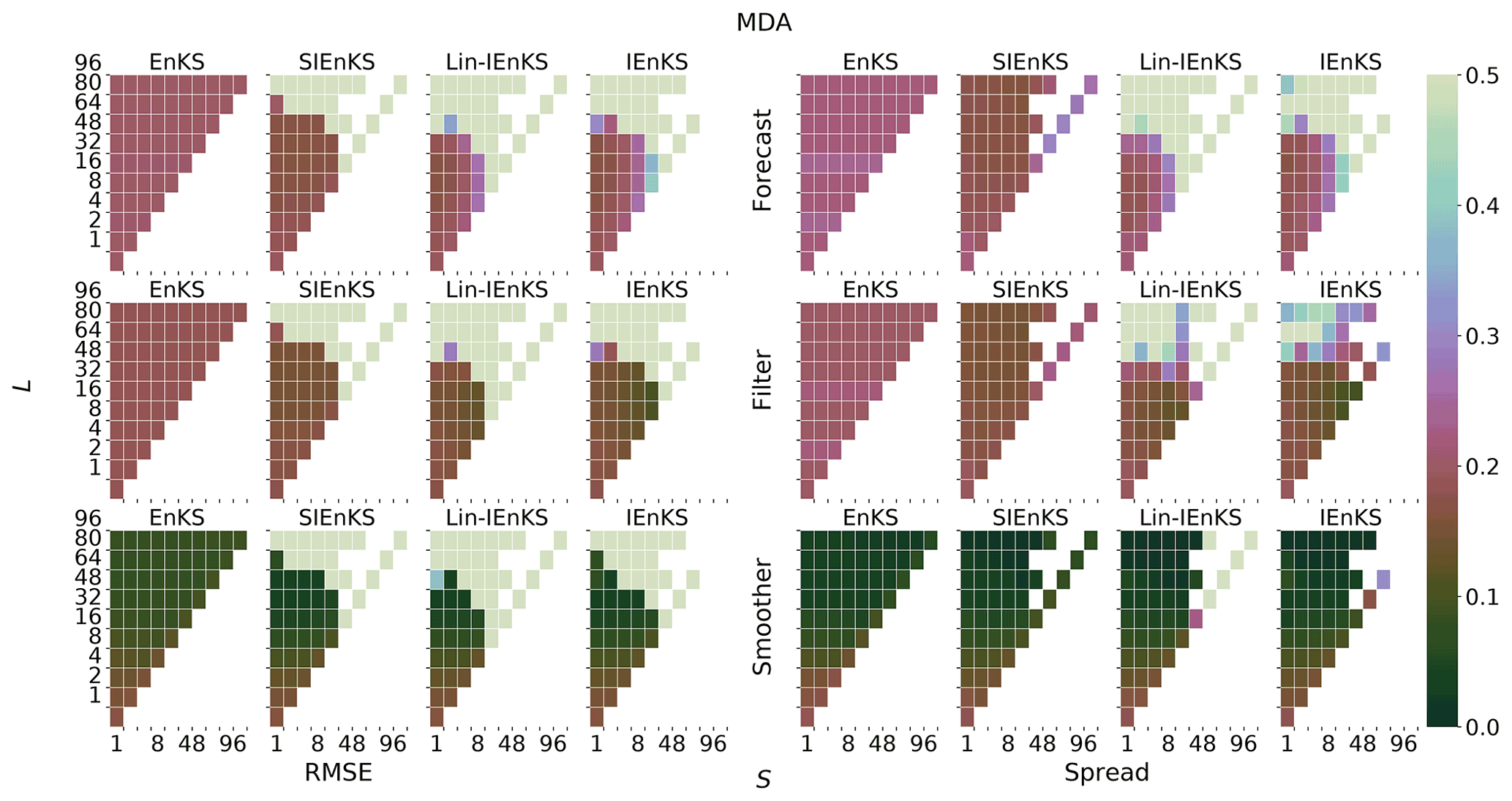
Figure 19 Lag length L on the vertical axis and shift S on the horizontal axis. MDA, tuned inflation, linear observations, ensemble size N_e=21, and Δt=0.05 are indicated. The EnKS SDA results are presented here for reference.

The SDA configuration is contrasted with Fig. 19, where we again see the apparent strengths of the SIEnKS MDA scheme. When MDA is introduced, all iterative schemes increase their respective stability regions to include longer lags and larger shifts in the DAW simultaneously. However, the SIEnKS has the largest stability region of all iterative estimators, extending to shifts at least as large as the other schemes for every lag setting. Likewise, the earlier distinction between the forecast and filter statistics of the SIEnKS and the 4D schemes is readily apparent. Not only does the stability region of the SIEnKS improve over the other schemes, but it is also generally more accurate in its predictive statistics at the end of long lag windows.

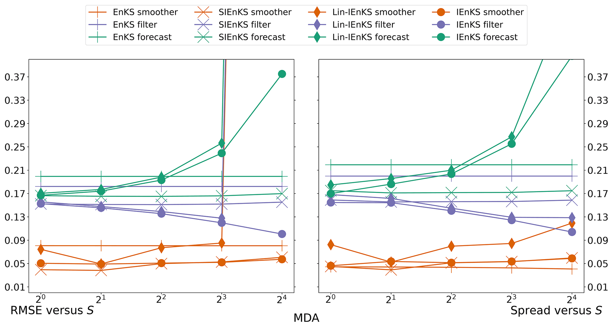
Figure 20 MDA configuration. RMSE and spread versus shift S. Lag L optimized for a minimum forecast RMSE in Fig. 19.

In order to obtain a finer picture of the effect of varying the shift S, we tune the lag and inflation simultaneously for each estimator for their minimal forecast RMSE when given a fixed shift; we plot the results of this tuning in Fig. 20. Given that all iterative estimators uniformly diverge for a shift S≥32, we only plot results for shifts in the range $\mathit{\{}{\mathrm{2}}^i{\mathit{\}}}_{i=\mathrm{0}}^{\mathrm{4}}$. Several important features stand out in this plot. First, note that, while optimizing the lag, the performance of the SIEnKS is almost invariant in the shift, similar to the performance of the EnKS. This is because the sequential filter analysis of the SIEnKS constrains the growth of the filter and forecast errors as the DAW shifts. Indeed, the prediction of states at times $t_{L-S+\mathrm{1}},\mathrm{\cdots },t_L$ arises from a filter ensemble at the previous time point. In the MDA scheme, the balancing weights for the observations of these newly introduced states in the DAW are, furthermore, all equal to one and equivalent to a standard ETKF filter analysis.

Second, note that the filter estimates of the (Lin-)IEnKS actually improve with larger shifts; however, this is an artifact of computing the filter statistics over all times $t_{L-S+\mathrm{1}},\mathrm{\cdots },t_L$ and using the observations ${\mathit{y}}_{L:L-S+\mathrm{1}}$ simultaneously. This means that the filter estimates for all times except t_L actually contain future information. This is contrasted with the sequential analyses of the EnKS and the SIEnKS, which only produce filter statistics with observations from past and current times.

Third, note that the Lin-IEnKS, while maintaining a similar prediction and filtering error to the IEnKS, is less stable and performs almost uniformly less accurately than the IEnKS in its smoothing estimates. The SIEnKS, moreover, tends to exhibit a slight improvement in stability and accuracy over the IEnKS therein.

Finally, it is immediately apparent how S>1 strongly increases the prediction error for the 4D estimators. The longer free forecasts for S>1, used to shift the DAW, accumulate errors such that, for S≥16, the Lin-IEnKS actually experiences filter divergence. The difference in the estimators' performances is once again a consequence of how observations are assimilated synchronously as in the EnKS/SIEnKS or asynchronously by default in the (Lin-)IEnKS.

Bearing all the above qualifications in mind, we analyze the performance of the estimators while varying the shift S. First, for all experimental settings, the leading-order cost of the SIEnKS MDA scheme is fixed at 2L ensemble simulations, whereas for the other schemes the minimal cost is at 2L+S ensemble simulations. For configurations where S>1, the SIEnKS thus makes a dramatic cost reduction versus the other schemes in this aspect alone, requiring fewer ensemble simulations per cycle. We consider that the leading-order cost for the Lin-IEnKS is similar to the SIEnKS for S=1, requiring only one more ensemble simulation per cycle. However, the SIEnKS with a shift S=16 maintains a prediction and smoother error that is comparable to the Lin-/IEnKS for a shift of S=1. This implies that the SIEnKS can maintain a performance similar to the S=1 IEnKS MDA scheme, while using $\mathrm{1}/\mathrm{16}$ of the total cycles needed by the IEnKS to pass over the same observations in real time. If we assume that the observations can be assimilated synchronously, then the above SIEnKS MDA scheme is thus able to run in its EnKS cycle over a long time series of observations while needing infrequent reinitialization with its smoothed estimates. For a real-time forecast cycle, where the computational cost/prediction accuracy tradeoff is the most important consideration, this once again demonstrates how the SIEnKS can balance this tradeoff, performing as well as, and often better than, 4D estimators with a substantially lower leading-order cost. Not only is each cycle less expensive in the SIEnKS than in the (Lin-)IEnKS, but the SIEnKS reduces the number of required cycles by an order of magnitude.

5.6 Strongly nonlinear forecast error dynamics – lag versus Δt

In all other numerical benchmarks, we focus on the scenario that the SIEnKS is designed for, i.e., DA cycles in which the forecast error evolution is weakly nonlinear. In this section, we demonstrate the limits of the SIEnKS when the forecast error dynamics dominate the nonlinearity of the DA cycle. We vary $\mathrm{\Delta }t\in \mathit{\{}\mathrm{0.05}\times i{\mathit{\}}}_{i=\mathrm{1}}^{\mathrm{10}}$, while the ensemble size N_e=21 and the shift S=1 are fixed. The lag is varied as $L\in \mathit{\{}\mathrm{1}+\mathrm{3}i{\mathit{\}}}_{i=\mathrm{0}}^{\mathrm{17}}$. We neglect the nonlinear observation operators in this section, though we include the finite size adaptive inflation formalism, which is itself designed to ameliorate the increasing nonlinearity in the forecast error dynamics. Single data assimilation and MDA configurations are considered for the iterative schemes as usual.

Figure 21 demonstrates the effect of the increasing nonlinearity of the forecast error evolution with tuned inflation. Due to the extreme nonlinearity for large Δt, we raise the heat map scale for the RMSE and spread to 1.0. Several features become apparent with the increasing forecast nonlinearity. First, the EnKS, which has a performance dependent on the standard ETKF cycle, is fully divergent for Δt≥0.2. This is in contrast with all iterative schemes which maintain adequate performance for Δt≤0.25. We note that the performance of the SIEnKS and the Lin-IEnKS, in this first scenario, is nearly identical; this corresponds to the fact that they are formally equivalent in this setting. However, appropriately, it is the 4D IEnKS that maintains the most stable and accurate performance over the range of forecast lengths. Indeed, this demonstrates the precise benefit of the iterative solution to 4D cost function for moderately nonlinear, non-Gaussian DA.

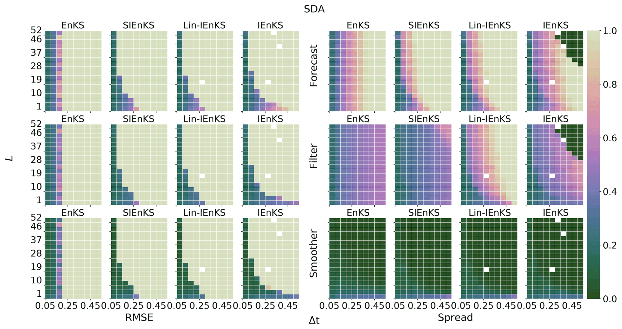
Figure 21 Lag length L on the vertical axis and Δt on the horizontal axis. SDA, tuned inflation, and ensemble size N_e=21 are indicated.

In Fig. 22, we repeat the same experiments as in Fig. 21 but using the finite size adaptive inflation, rather than tuned inflation, for each estimator. Once again, the efficacy of the finite size formalism in ameliorating the nonlinearity of the forecast error dynamics is demonstrated. In particular, all schemes except the SIEnKS see an overall improvement in their stability region and often in their overall accuracy. The EnKS-N actually strongly outperforms the tuned inflation EnKS, extending an adequate filter performance as far as Δt≤0.35. Likewise, the IEnKS-N has a strongly enhanced stability region, though it increasingly suffers from catastrophic filter divergence outside of this zone. Notably, whereas the SIEnKS-N outperformed the Lin-IEnKS-N for Δt=0.05, the Lin-IEnKS-N generally yields a better performance for moderately to strongly nonlinear forecast error dynamics. Indeed, the finite size formalism appears to become incompatible with the design of the SIEnKS for strongly nonlinear forecast error dynamics, as suggested by the widespread ensemble collapse and catastrophic divergence.

Figure 22 Lag length L on the vertical axis and Δt on the horizontal axis. SDA, adaptive inflation, and ensemble size N_e=21 are indicated.

As a final experimental configuration, we consider how MDA affects the increasing nonlinearity of the forecast error dynamics. Figure 23 demonstrates the performance of these estimators in the MDA configuration with tuned inflation, where the SDA results of the EnKS are pictured for reference. In particular, we see the usual increase in the estimators' stability regions over the SDA configuration. However, the improvement in the SIEnKS over the Lin-IEnKS is marginal to nonexistent for moderately to strongly nonlinear forecast error dynamics. The 4D IEnKS, furthermore, is again the estimator with the largest stability region and greatest accuracy over a wide range of Δt.

Figure 23 Lag length L on the vertical axis and Δt on the horizontal axis. MDA, tuned inflation, and ensemble size N_e=21 are indicated.

The results in this section indicate that, while the SIEnKS is very successful in weakly nonlinear forecast error dynamics, the approximations used in this estimator strongly depend on the source of nonlinearity in the DA cycle. Particularly, when the nonlinearity of the forecast error dynamics dominates the DA cycle, the approximations of the SIEnKS break down. It is thus favorable to consider the Lin-IEnKS, or to set a low threshold for the iterations in the IEnKS, instead of applying the SIEnKS in this regime. Notably, as the finite size inflation formalism is designed for a scenario different to that of the SIEnKS, one may instead consider designing adaptive covariance inflation in such a way that it exploits the design principles of the SIEnKS. Such a study goes beyond the scope of this work and will be considered later.

6 Conclusions

In this work, we achieve three primary objectives. First, we provide a review of sequential, ensemble variational Kalman filters and smoothers with perfect model assumptions within the Bayesian MAP formalism of the IEnKS. Second, we rigorously derive our single-iteration formalism as a novel approximation of the Bayesian MAP estimation, explaining how this relates to other well-known smoothing schemes and how its design is differentiated in a variety of contexts. Third, using the numerical framework of DataAssimilationBenchmarks.jl (Grudzien et al., 2021), we extensively demonstrate how the SIEnKS has a unique advantage in balancing the computational cost/prediction accuracy tradeoff in short-range forecast applications. Pursuant to this, we provide a cost analysis and pseudo-code for all of the schemes studied in this work, in addition to the open-source implementations available in the supporting Julia package. Together, this work provides a practical reference for a variety of topics at the state of the art in ensemble variational Kalman smoothing.

The rationale of the SIEnKS is, once again, to efficiently perform a Bayesian MAP estimation in real-time, short-range forecast applications where the forecast error dynamics is weakly nonlinear. Our central result is the novel SIEnKS MDA scheme, which not only improves the forecast accuracy and analysis stability in this regime but also simultaneously reduces the leading-order cost versus the traditional 4D MDA approach. This MDA scheme is demonstrated to produce significant performance advantages in the simple setting where there is a linear observation operator and especially when the shift S can be taken greater than one. Not only is each cycle of the SIEnKS MDA scheme significantly less expensive than the other estimators for S>1, but the estimator performance while varying S tends to be invariant. This crucial aspect also means that one can, in principle, reduce the number of cycles actually needed by the estimator to produce forecasts in real time. Our scheme also appears better equipped than the 4D MDA estimation to handle highly nonlinear observation operators, as it maintains greater accuracy and is more robust to the effects of local minima. Separately, we find that, in our target regime, the single-iteration formalism is cost-effective for optimizing hyperparameters of the estimation scheme, as with the SIEnKS-N.

The above successes of the SIEnKS come with the following three important qualifications: (i) we have focused on synchronous DA, assuming that we can sequentially assimilate observations before producing a prediction step, (ii) we have not studied localization or hybridization, which are widely used in ensemble-based estimators to overcome the curse of dimensionality for realistic geophysical models, and (iii) we have relied upon the perfect model assumption, whereas realistic forecast settings include significant modeling errors. These restrictions come by necessity, to limit the scope of an already lengthy study. However, we note that the SIEnKS is capable of asynchronous DA, as already discussed in Sect. 4.4. Likewise, it is possible that some of the issues faced by the IEnKS in integrating localization/hybridization (Bocquet, 2016) may actually be ameliorated by the design principles of the SIEnKS. Domain localization, as in the LETKF (Hunt et al., 2007; Sakov and Bertino, 2011), is likely to have a satisfactory extension to the SIEnKS, where this may be applied directly in the filter step as usual. Assuming that the ensemble forecast dynamics is not highly nonlinear, the spatial correlations defining the observation domain truncation for the initial ensemble at t₀ may, furthermore, be well approximated by the domains from the filter step but mapped by a linear, reverse-time evolution over the DAW via an explicit or implicit adjoint model. Experiments suggest that a tuned radius for a smoother domain localization can be implemented successfully in an EnKS analysis (Nerger et al., 2014). However, there are also rich opportunities to iteratively optimize a localization hyperparameter as with, e.g., the α trick (Lorenc, 2003) within the SIEnKS framework. Similarly, it is possible that an extension of the single-iteration formalism could provide a novel alternative to other iterative ensemble smoothers designed for model error, such as the IEnKS-Q (Sakov et al., 2018; Fillion et al., 2020), EnKS expectation maximization schemes (Pulido et al., 2018), or the family of OSA smoothers (Ait-El-Fquih and Hoteit, 2022).

For the reasons above, this initial study provides a number of directions in which our single-iteration formalism can be extended. Localization and hybridization are both prime targets to translate the benefits of the SIEnKS to an operational short-range forecasting setting. Likewise, an asynchronous DA design is an important operational topic for this estimator. Noting that the finite size adaptive inflation formalism is designed to perform in a different regime than the SIEnKS and is not fully compatible with MDA schemes, developing an adaptive inflation and/or model error estimation based on the design principles of the SIEnKS is an important direction for a future study. Having currently demonstrated the initial success of this single-iteration formalism, each of these above directions can be considered in a devoted work. We hope that the framework provided in this paper will guide these future studies and will provide a robust basis of comparison for further development of ensemble variational Kalman filters and smoothers.

Appendix A: Algorithm pseudo-code

Algorithm A1 Ensemble transform (ET).

Require:

Ensemble matrix $\mathbf{E}\in {\mathbb{R}}^{N_x\times N_{\mathrm{e}}}$, observation map ℋ, observation error covariance $\mathbf{R}\in {\mathbb{R}}^{N_y\times N_y}$, and observation vector y

1:

Y=ℋ(E)

2:

$\widehat{\mathit{y}}=\mathbf{Y}\mathbf{1}/N_{\mathrm{e}}$

3:

$\mathbf{S}={\mathbf{R}}^{-\frac{\mathrm{1}}{\mathrm{2}}}\left(\mathbf{Y}-\widehat{\mathit{y}}{\mathbf{1}}^{\top }\right)$

4:

$\widehat{\mathit{\delta }}={\mathbf{R}}^{-\frac{\mathrm{1}}{\mathrm{2}}}\left(\mathit{y}-\widehat{\mathit{y}}\right)$

5:

$\mathrm{\nabla }\stackrel{\mathrm{̃}}{\mathcal{J}}=-{\mathbf{S}}^{\top }\widehat{\mathit{\delta }}$

6:

${\stackrel{\mathrm{̃}}{\mathbf{\Xi }}}_{\stackrel{\mathrm{̃}}{\mathcal{J}}}=(N_{\mathrm{e}}-\mathrm{1}){\mathbf{I}}_{N_{\mathrm{e}}}+{\mathbf{S}}^{\top }\mathbf{S}$

7:

$\mathit{w}=-{\stackrel{\mathrm{̃}}{\mathbf{\Xi }}}_{\stackrel{\mathrm{̃}}{\mathcal{J}}}^{-\mathrm{1}}\mathrm{\nabla }\stackrel{\mathrm{̃}}{\mathcal{J}}$

8:

$\mathbf{T}={\stackrel{\mathrm{̃}}{\mathbf{\Xi }}}_{\stackrel{\mathrm{̃}}{\mathcal{J}}}^{-\frac{\mathrm{1}}{\mathrm{2}}}$

9:

return  T,w

Algorithm A2 Random mean-preserving orthogonal matrix (RO).

Require:

Ensemble size N_e; let QR represent the QR algorithm.

1:

Let $\mathbf{Q}\in {\mathbb{R}}^{(N_{\mathrm{e}}-\mathrm{1})\times (N_{\mathrm{e}}-\mathrm{1})}$, with entries drawn iid from 𝒩(0,1)

2:

$\mathbf{Q},\mathbf{R}=\mathrm{QR}\left(\mathbf{Q}\right)$

3:

$\mathbf{U}=\left(\begin{array}{cc}\mathrm{1}& \mathrm{0}\\ \mathrm{0}& \mathbf{Q}\end{array}\right)$

4:

Let $\mathit{\{}{\mathit{a}}_i{\mathit{\}}}_{i=\mathrm{1}}^{N_{\mathrm{e}}}$ be an arbitrary orthogonal basis of ${\mathbb{R}}^{N_{\mathrm{e}}}$ up to the requirement that ${\mathit{a}}_{\mathrm{1}}=\mathbf{1}/\sqrt{N_{\mathrm{e}}}$; let $\mathbf{A}=[{\mathit{a}}_i{]}_{i=\mathrm{1}}^{N_{\mathrm{e}}}$

5:

return  $\mathbf{U}={\mathbf{AUA}}^{\top }$

Algorithm A3 Ensemble update (EU).

Require:

Ensemble matrix $\mathbf{E}\in {\mathbb{R}}^{N_x\times N_{\mathrm{e}}}$, transform T, weights w, and mean-preserving orthogonal matrix U.

1:

$\widehat{\mathit{x}}=\mathbf{E}\mathbf{1}/N_{\mathrm{e}}$

2:

$\mathbf{X}=\mathbf{E}-\widehat{\mathit{x}}{\mathbf{1}}^{\top }$

3:

return  $\mathbf{E}=\widehat{\mathit{x}}{\mathbf{1}}^{\top }+\mathbf{X}\left(\mathit{w}{\mathbf{1}}^{\top }+\sqrt{N_{\mathrm{e}}-\mathrm{1}}\mathbf{TU}\right)$

Algorithm A4 Covariance inflation (CI).

Require:

Ensemble matrix $\mathbf{E}\in {\mathbb{R}}^{N_x\times N_{\mathrm{e}}}$ and inflation λ.

1:

$\widehat{\mathit{x}}=\mathbf{E}\mathbf{1}/N_{\mathrm{e}}$

2:

$\mathbf{X}=\mathbf{E}-\widehat{\mathit{x}}{\mathbf{1}}^{\top }$

3:

return  $\mathbf{E}=\widehat{\mathit{x}}{\mathbf{1}}^{\top }+\mathit{\lambda }\mathbf{X}$

Algorithm A5 ETKF.

Require:

Observation y₁, filter ensemble ${\mathbf{E}}_{\mathrm{0}}^{\mathrm{filt}}\in {\mathbb{R}}^{N_x\times N_{\mathrm{e}}}$, and inflation λ.

Require:

Let ET, RO, EU, and CI represent Algorithms A1, A2, A3, and A4, respectively.

1:

${\mathbf{E}}_{\mathrm{1}}^{\mathrm{fore}}={\mathcal{M}}_{\mathrm{1}}\left({\mathbf{E}}_{\mathrm{0}}^{\mathrm{filt}}\right)$

2:

$\mathbf{T},\mathit{w}=\mathrm{ET}\left({\mathbf{E}}_{\mathrm{1}}^{\mathrm{fore}},{\mathcal{H}}_{\mathrm{1}},{\mathbf{R}}_{\mathrm{1}},{\mathit{y}}_{\mathrm{1}}\right)$

3:

U=RO(N_e)

4:

${\mathbf{E}}_{\mathrm{1}}^{\mathrm{filt}}=\mathrm{EU}\left({\mathbf{E}}_{\mathrm{1}}^{\mathrm{fore}},\mathbf{T},\mathit{w},\mathbf{U}\right)$

5:

${\mathbf{E}}_{\mathrm{1}}^{\mathrm{filt}}=\mathrm{CI}\left({\mathbf{E}}_{\mathrm{1}}^{\mathrm{filt}},\mathit{\lambda }\right)$

Require:

Store ${\mathbf{E}}_{\mathrm{0}}^{\mathrm{filt}}:={\mathbf{E}}_{\mathrm{1}}^{\mathrm{filt}}$ for the next cycle

Algorithm A6 EnKS.

Require:

Lag=L, shift=S, observations ${\mathit{y}}_{L:L-S+\mathrm{1}}$, smoother ensemble states ${\mathbf{E}}_{L-S:\mathrm{0}}^{\mathrm{smth}}$, ensemble size N_e, and inflation λ.

Require:

Let ET, RO, EU, and CI represent Algorithms A1, A2, A3, and A4, respectively.

1:

${\mathbf{E}}_{L-S}^{\mathrm{filt}}:={\mathbf{E}}_{L-S}^{\mathrm{smth}}$

2:

for $k\in \mathit{\{}L-S+\mathrm{1},\mathrm{\cdots },L\mathit{\}}$ do

3:

${\mathbf{E}}_k^{\mathrm{fore}}={\mathcal{M}}_k\left({\mathbf{E}}_{k-\mathrm{1}}^{\mathrm{filt}}\right)$

4:

$\mathbf{T},\mathit{w}=\mathrm{ET}\left({\mathbf{E}}_k^{\mathrm{fore}},{\mathcal{H}}_k,{\mathbf{R}}_k,{\mathit{y}}_k\right)$

5:

U=RO(N_e)

6:

${\mathbf{E}}_k^{\mathrm{filt}}=\mathrm{EU}\left({\mathbf{E}}_k^{\mathrm{fore}},\mathbf{T},\mathit{w},\mathbf{U}\right)$

7:

for  $j\in \mathit{\{}\mathrm{0},\mathrm{\cdots },k-\mathrm{1}\mathit{\}}$ do

8:

${\mathbf{E}}_j^{\mathrm{smth}}=\mathrm{EU}\left({\mathbf{E}}_j^{\mathrm{smth}},\mathbf{T},\mathit{w},\mathbf{U}\right)$

9:

end for

10:

${\mathbf{E}}_k^{\mathrm{filt}}=\mathrm{CI}\left({\mathbf{E}}_k^{\mathrm{filt}},\mathit{\lambda }\right)$

11:

${\mathbf{E}}_k^{\mathrm{smth}}:={\mathbf{E}}_k^{\mathrm{filt}}$

12:

end for

Require:

Store ${\mathbf{E}}_{L-S:\mathrm{0}}^{\mathrm{smth}}:={\mathbf{E}}_{L:S}^{\mathrm{smth}}$ for the next cycle

Algorithm A7 Gauss–Newton IEnKS in the SDA transform version.

Require:

Lag =L, shift =S, and observations ${\mathit{y}}_{L:L-S+\mathrm{1}}$.

Require:

${\mathbf{E}}_{\mathrm{0}}^{\mathrm{smth}}\in {\mathbb{R}}^{N_{\mathrm{e}}\times N_{\mathrm{e}}}$

Require:

Let RO, EU, and CI represent algorithms A2, A3, and A4, respectively.

Require:

Parameters tol, j_max, inflation λ.

1:

$\mathbf{T}:={\mathbf{I}}_{N_{\mathrm{e}}}$

2:

${\mathbf{E}}_{\mathrm{0}}:={\mathbf{E}}_{\mathrm{0}}^{\mathrm{smth}}$

3:

$j:=\mathrm{0},\mathit{w}:=\mathbf{0}$

4:

loop

5:

for $k\in \mathit{\{}\mathrm{1},\mathrm{\cdots },L\mathit{\}}$ do

6:

${\mathbf{E}}_k={\mathcal{M}}_k\left({\mathbf{E}}_{k-\mathrm{1}}\right)$

7:

if $k\in \mathit{\{}L-S+\mathrm{1},\mathrm{\cdots },L\mathit{\}}$ then

8:

Y_k=ℋ_k(E_k)

9:

${\widehat{\mathit{y}}}_k={\mathbf{Y}}_k\mathbf{1}/N_{\mathrm{e}}$

10:

${\mathbf{S}}_k={\mathbf{R}}_k^{-\frac{\mathrm{1}}{\mathrm{2}}}\left({\mathbf{Y}}_k-{\widehat{\mathit{y}}}_k{\mathbf{1}}^{\top }\right){\mathbf{T}}^{-\mathrm{1}}$

11:

${\widehat{\mathit{\delta }}}_k={\mathbf{R}}_k^{-\frac{\mathrm{1}}{\mathrm{2}}}\left({\mathit{y}}_k-{\widehat{\mathit{y}}}_k\right)$

12:

end if

13:

end for

14:

$\mathrm{\nabla }\stackrel{\mathrm{̃}}{\mathcal{J}}=(N_{\mathrm{e}}-\mathrm{1})\mathit{w}-{\sum }_{k=L-S+\mathrm{1}}^L{\mathbf{S}}_k^{\top }{\widehat{\mathit{\delta }}}_k$

15:

${\stackrel{\mathrm{̃}}{\mathbf{\Xi }}}_{\stackrel{\mathrm{̃}}{\mathcal{J}}}=(N_{\mathrm{e}}-\mathrm{1}){\mathbf{I}}_{N_{\mathrm{e}}}+{\sum }_{k=L-S+\mathrm{1}}^L{\mathbf{S}}_k^{\top }{\mathbf{S}}_k$

16:

$\mathrm{\Delta }\mathit{w}={\stackrel{\mathrm{̃}}{\mathbf{\Xi }}}_{\stackrel{\mathrm{̃}}{\mathcal{J}}}^{-\mathrm{1}}\mathrm{\nabla }\stackrel{\mathrm{̃}}{\mathcal{J}}$

17:

$\mathit{w}:=\mathit{w}-\mathrm{\Delta }\mathit{w}$

18:

$j:=j+\mathrm{1}$

19:

if $\parallel \mathrm{\Delta }\mathit{w}\parallel <\mathrm{tol}$ or j=j_max then

20:

break loop

21:

else

22:

$\mathbf{T}={\stackrel{\mathrm{̃}}{\mathbf{\Xi }}}_{\stackrel{\mathrm{̃}}{\mathcal{J}}}^{-\frac{\mathrm{1}}{\mathrm{2}}}$

23:

${\mathbf{E}}_{\mathrm{0}}=\mathrm{EU}\left({\mathbf{E}}_{\mathrm{0}}^{\mathrm{smth}},\mathbf{T},\mathit{w},{\mathbf{I}}_{N_{\mathrm{e}}}\right)$

24:

end if

25:

end loop

26:

$\mathbf{T}={\stackrel{\mathrm{̃}}{\mathbf{\Xi }}}_{\stackrel{\mathrm{̃}}{\mathcal{J}}}^{-\frac{\mathrm{1}}{\mathrm{2}}}$

27:

U=RO(N)

28:

${\mathbf{E}}_{\mathrm{0}}:=\mathrm{EU}\left({\mathbf{E}}_{\mathrm{0}}^{\mathrm{smth}},\mathbf{T},\mathit{w},\mathbf{U}\right)$

29:

for $k=\mathrm{1},\mathrm{\cdots },L+S$ do

30:

${\mathbf{E}}_k={\mathcal{M}}_k\left({\mathbf{E}}_{k-\mathrm{1}}\right)$

31:

end for

32:

${\mathbf{E}}_{L-S:\mathrm{0}}^{\mathrm{smth}}:={\mathbf{E}}_{L-S:\mathrm{0}}$

33:

${\mathbf{E}}_{L:L-S+\mathrm{1}}^{\mathrm{filt}}:={\mathbf{E}}_{L:L-S+\mathrm{1}}$

34:

${\mathbf{E}}_{L+S:L+\mathrm{1}}^{\mathrm{fore}}:={\mathbf{E}}_{L+S:L+\mathrm{1}}$

35:

${\mathbf{E}}_S^{\mathrm{smth}}=\mathrm{CI}\left({\mathbf{E}}_S^{\mathrm{smth}},\mathit{\lambda }\right)$

Require:

${\mathbf{E}}_{\mathrm{0}}^{\mathrm{smth}}:={\mathbf{E}}_S^{\mathrm{smth}}$ for the next cycle.

Algorithm A8 SIEnKS in the SDA version.

Require:

Lag =L, shift =S, observations ${\mathit{y}}_{L:L-S+\mathrm{1}}$, ensemble states ${\mathbf{E}}_{\mathrm{0}}^{\mathrm{smth}}$ and ${\mathbf{E}}_{L-S}^{\mathrm{smth}}$, and inflation λ.

Require:

Let ET, RO, EU, and CI represent Algorithms A1, A2, A3, and A4, respectively.

1:

${\mathbf{E}}_{L-S}^{\mathrm{filt}}:={\mathbf{E}}_{L-S}^{\mathrm{smth}}$

2:

for $k\in \mathit{\{}L-S+\mathrm{1},\mathrm{\cdots },L\mathit{\}}$ do

3:

${\mathbf{E}}_k^{\mathrm{fore}}={\mathcal{M}}_k\left({\mathbf{E}}_{k-\mathrm{1}}^{\mathrm{filt}}\right)$

4:

$\mathbf{T},\mathit{w}=\mathrm{ET}\left({\mathbf{E}}_k^{\mathrm{fore}},{\mathcal{H}}_k,{\mathbf{R}}_k,{\mathit{y}}_k\right)$

5:

U_k=RO(N)

6:

${\mathbf{E}}_k^{\mathrm{filt}}=\mathrm{EU}\left({\mathbf{E}}_k^{\mathrm{fore}},\mathbf{T},\mathit{w},{\mathbf{U}}_k\right)$

7:

${\mathbf{E}}_{\mathrm{0}}^{\mathrm{smth}}=\mathrm{EU}\left({\mathbf{E}}_{\mathrm{0}}^{\mathrm{smth}},\mathbf{T},\mathit{w},{\mathbf{U}}_k\right)$

8:

end for

9:

${\mathbf{E}}_{\mathrm{0}}^{\mathrm{smth}}:=\mathrm{CI}\left({\mathbf{E}}_{\mathrm{0}}^{\mathrm{smth}},\mathit{\lambda }\right)$

10:

for $k=\mathrm{1},\mathrm{\cdots },L$ do

11:

${\mathbf{E}}_k^{\mathrm{smth}}={\mathcal{M}}_k^{\mathrm{smth}}\left({\mathbf{E}}_{k-\mathrm{1}}\right)$

12:

end for

Require:

${\mathbf{E}}_{\mathrm{0}}^{\mathrm{smth}}:={\mathbf{E}}_S^{\mathrm{smth}}$, ${\mathbf{E}}_{L-S}^{\mathrm{smth}}:={\mathbf{E}}_L^{\mathrm{smth}}$ for the next cycle.

Algorithm A9 Maximum likelihood ensemble transform (MLET).

Require:

Ensemble matrix $\mathbf{E}\in {\mathbb{R}}^{N_x\times N_{\mathrm{e}}}$, observation map ℋ, observation error covariance $\mathbf{R}\in {\mathbb{R}}^{N_y\times N_y}$, and observation vector y.

Require:

Parameters tol,j_max

1:

$\mathbf{T}:={\mathbf{I}}_{N_{\mathrm{e}}}$

2:

$j:=\mathrm{0},\mathit{w}:=\mathbf{0}$

3:

E₀:=E

4:

loop

5:

Y=ℋ(E)

6:

$\widehat{\mathit{y}}=\mathbf{Y}\mathbf{1}/N_{\mathrm{e}}$

7:

$\mathbf{S}={\mathbf{R}}^{-\frac{\mathrm{1}}{\mathrm{2}}}\left(\mathbf{Y}-\widehat{\mathit{y}}{\mathbf{1}}^{\top }\right){\mathbf{T}}^{-\mathrm{1}}$

8:

$\widehat{\mathit{\delta }}={\mathbf{R}}^{-\frac{\mathrm{1}}{\mathrm{2}}}\left(\mathit{y}-\widehat{\mathit{y}}\right)$

9:

$\mathrm{\nabla }\stackrel{\mathrm{̃}}{\mathcal{J}}=(N_{\mathrm{e}}-\mathrm{1})\mathit{w}-{\mathbf{S}}^{\top }\widehat{\mathit{\delta }}$

10:

${\stackrel{\mathrm{̃}}{\mathbf{\Xi }}}_{\stackrel{\mathrm{̃}}{\mathcal{J}}}=(N_{\mathrm{e}}-\mathrm{1}){\mathbf{I}}_{N_{\mathrm{e}}}+{\mathbf{S}}^{\top }\mathbf{S}$

11:

$\mathrm{\Delta }\mathit{w}={\stackrel{\mathrm{̃}}{\mathbf{\Xi }}}_{\stackrel{\mathrm{̃}}{\mathcal{J}}}^{-\mathrm{1}}\mathrm{\nabla }\stackrel{\mathrm{̃}}{\mathcal{J}}$

12:

$\mathit{w}:=\mathit{w}-\mathrm{\Delta }\mathit{w}$

13:

if $\parallel \mathrm{\Delta }\mathit{w}\parallel <\mathrm{tol}$ or j=j_max then

14:

break loop

15:

else

16:

$\mathbf{T}={\stackrel{\mathrm{̃}}{\mathbf{\Xi }}}_{\stackrel{\mathrm{̃}}{\mathcal{J}}}^{-\frac{\mathrm{1}}{\mathrm{2}}}$

17:

$\mathbf{E}=\mathrm{EU}\left({\mathbf{E}}_{\mathrm{0}},\mathbf{T},\mathit{w},{\mathbf{I}}_{N_{\mathrm{e}}}\right)$

18:

end if

19:

end loop

20:

$\mathbf{T}={\stackrel{\mathrm{̃}}{\mathbf{\Xi }}}_{\stackrel{\mathrm{̃}}{\mathcal{J}}}^{-\frac{\mathrm{1}}{\mathrm{2}}}$

21:

return  T,w

Algorithm A10 Finite size ensemble transform (FSET).

Require:

Ensemble matrix $\mathbf{E}\in {\mathbb{R}}^{N_x\times N_{\mathrm{e}}}$, observation map ℋ, observation error covariance $\mathbf{R}\in {\mathbb{R}}^{N_y\times N_y}$, and observation vector y.

Require:

Parameters tol,j_max

1:

$\mathbf{T}:={\mathbf{I}}_{N_{\mathrm{e}}}$

2:

$j:=\mathrm{0},\mathit{w}:=\mathbf{0}$

3:

E₀:=E

4:

${\mathit{ϵ}}_{N_{\mathrm{e}}}:=\mathrm{1}+\mathrm{1}/N_{\mathrm{e}}$, $N_{\mathrm{eff}}:=N_e+\mathrm{1}$

5:

loop

6:

Y=ℋ(E)

7:

$\widehat{\mathit{y}}=\mathbf{Y}\mathbf{1}/N_{\mathrm{e}}$

8:

$\mathbf{S}={\mathbf{R}}^{-\frac{\mathrm{1}}{\mathrm{2}}}\left(\mathbf{Y}-\widehat{\mathit{y}}{\mathbf{1}}^{\top }\right){\mathbf{T}}^{-\mathrm{1}}$

9:

$\widehat{\mathit{\delta }}={\mathbf{R}}^{-\frac{\mathrm{1}}{\mathrm{2}}}\left(\mathit{y}-\widehat{\mathit{y}}\right)$

10:

$\mathit{\zeta }=\mathrm{1}/\left({\mathit{ϵ}}_{N_{\mathrm{e}}}+{\mathit{w}}^{\top }\mathit{w}\right)$

11:

$\mathrm{\nabla }\stackrel{\mathrm{̃}}{\mathcal{J}}=\mathit{\zeta }\left(N_{\mathrm{eff}}\right)\mathit{w}-{\mathbf{S}}^{\top }\widehat{\mathit{\delta }}$

12:

${\stackrel{\mathrm{̃}}{\mathbf{\Xi }}}_{\stackrel{\mathrm{̃}}{\mathcal{J}}}=(N_{\mathrm{e}}-\mathrm{1}){\mathbf{I}}_{N_{\mathrm{e}}}+{\mathbf{S}}^{\top }\mathbf{S}$

13:

$\mathrm{\Delta }\mathit{w}={\stackrel{\mathrm{̃}}{\mathbf{\Xi }}}_{\stackrel{\mathrm{̃}}{\mathcal{J}}}^{-\mathrm{1}}\mathrm{\nabla }\stackrel{\mathrm{̃}}{\mathcal{J}}$

14:

$\mathit{w}:=\mathit{w}-\mathrm{\Delta }\mathit{w}$

15:

$j:=j+\mathrm{1}$

16:

if $\parallel \mathrm{\Delta }\mathit{w}\parallel <\mathrm{tol}$ or j=j_max then

17:

break loop

18:

else

19:

$\mathbf{T}={\stackrel{\mathrm{̃}}{\mathbf{\Xi }}}_{\stackrel{\mathrm{̃}}{\mathcal{J}}}^{-\frac{\mathrm{1}}{\mathrm{2}}}$

20:

$\mathbf{E}=\mathrm{EU}\left({\mathbf{E}}_{\mathrm{0}},\mathbf{T},\mathit{w},{\mathbf{I}}_{N_{\mathrm{e}}}\right)$

21:

end if

22:

end loop

23:

$\mathit{\zeta }=\mathrm{1}/\left({\mathit{ϵ}}_N+{\mathit{w}}^{\top }\mathit{w}\right)$

24:

${\stackrel{\mathrm{̃}}{\mathbf{\Xi }}}_{\stackrel{\mathrm{̃}}{\mathcal{J}}}=N_{\mathrm{eff}}\left(\mathit{\zeta }{\mathbf{I}}_N-\mathrm{2}{\mathit{\zeta }}^{\mathrm{2}}\mathit{w}{\mathit{w}}^{\top }\right)+{\mathbf{S}}^{\top }\mathbf{S}$

25:

$\mathbf{T}={\stackrel{\mathrm{̃}}{\mathbf{\Xi }}}_{\stackrel{\mathrm{̃}}{\mathcal{J}}}^{-\frac{\mathrm{1}}{\mathrm{2}}}$

26:

return  T,w

Algorithm A11 Gauss–Newton IEnKS-N in the SDA transform version.

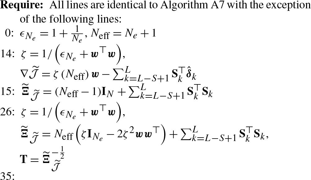
Algorithm A12 SIEnKS in the MDA version.

Require:

Lag=L, shift=S, observations y_L:1, MDA conditional ensemble ${\mathbf{E}}_{\mathrm{0}}^{\mathrm{mda}}$, ensemble size N_e, and inflation λ.

Require:

Let ET, RO, EU, and CI represent Algorithms A1, A2, A3 and A4, respectively.

Require:

Let $\mathit{\{}{\mathit{\beta }}_k{\mathit{\}}}_{k=\mathrm{1}}^L$ and $\mathit{\{}{\mathit{\eta }}_k{\mathit{\}}}_{k=\mathrm{1}}^L$ be the multiple data assimilation and balancing weights, respectively.

1:

${\mathbf{E}}_{\mathrm{0}}^{\mathrm{bal}}:={\mathbf{E}}_{\mathrm{0}}^{\mathrm{mda}}$

2:

for $k=\mathrm{1},\mathrm{\cdots },L$ do

3:

U=RO(N_e)

4:

${\mathbf{E}}_k^{\mathrm{bal}}={\mathcal{M}}_k\left({\mathbf{E}}_{k-\mathrm{1}}^{\mathrm{bal}}\right)$

5:

if $k\in \mathit{\{}L-S+\mathrm{1},\mathrm{\cdots },L\mathit{\}}$ then

6:

${\mathbf{E}}_k^{\mathrm{fore}}:={\mathbf{E}}_k^{\mathrm{bal}}$

7:

end if

8:

$\mathbf{T},\mathit{w}=\mathrm{ET}\left({\mathbf{E}}_k^{\mathrm{bal}},{\mathcal{H}}_k,{\mathbf{R}}_k/{\mathit{\eta }}_k,{\mathit{y}}_k\right)$

9:

${\mathbf{E}}_k^{\mathrm{bal}}=\mathrm{EU}\left({\mathbf{E}}_j^{\mathrm{bal}},\mathbf{T},\mathit{w},\mathbf{U}\right)$

10:

if $k\in \mathit{\{}L-S+\mathrm{1},\mathrm{\cdots }L\mathit{\}}$ then

11:

${\mathbf{E}}_k^{\mathrm{filt}}:={\mathbf{E}}_k^{\mathrm{bal}}$

12:

end if

13:

for $j=\mathrm{0},\mathrm{\cdots },k-\mathrm{1}$ do

14:

${\mathbf{E}}_j^{\mathrm{bal}}=\mathrm{EU}\left({\mathbf{E}}_j^{\mathrm{bal}},\mathbf{T},\mathit{w},\mathbf{U}\right)$

15:

end for

16:

if k=S then

17:

${\mathbf{E}}_{\mathrm{0}}^{\mathrm{mda}}={\mathbf{E}}_{\mathrm{0}}^{\mathrm{bal}}$

18:

${\mathbf{E}}_S^{\mathrm{mda}}={\mathbf{E}}_k^{\mathrm{bal}}$

19:

end if

20:

end for

21:

${\mathbf{E}}_{\mathrm{0}:L-S}^{\mathrm{smth}}:={\mathbf{E}}_{\mathrm{0}:L-S}^{\mathrm{bal}}$

22:

for $k=S+\mathrm{1},\mathrm{\cdots },L$ do

23:

U=RO(N_e)

24:

${\mathbf{E}}_k^{\mathrm{mda}}={\mathcal{M}}_k\left({\mathbf{E}}_{k-\mathrm{1}}^{\mathrm{mda}}\right)$

25:

$\mathbf{T},\mathit{w}=\mathrm{ET}\left({\mathbf{E}}_k^{\mathrm{mda}},{\mathcal{H}}_k,{\mathbf{R}}_k/{\mathit{\beta }}_k,{\mathit{y}}_k\right)$

26:

${\mathbf{E}}_k^{\mathrm{mda}}=\mathrm{EU}\left({\mathbf{E}}_k^{\mathrm{mda}},\mathbf{T},\mathit{w},\mathbf{U}\right)$

27:

${\mathbf{E}}_{\mathrm{0}}^{\mathrm{mda}}=\mathrm{EU}\left({\mathbf{E}}_{\mathrm{0}}^{\mathrm{mda}},\mathbf{T},\mathit{w},\mathbf{U}\right)$

28:

end for

29:

${\mathbf{E}}_{\mathrm{0}}^{\mathrm{mda}}=\mathrm{CI}\left({\mathbf{E}}_{\mathrm{0}}^{\mathrm{mda}},\mathit{\lambda }\right)$

30:

for $k=\mathrm{1},\mathrm{\cdots },S$ do

31:

${\mathbf{E}}_k^{\mathrm{mda}}={\mathcal{M}}_k\left({\mathbf{E}}_{k-\mathrm{1}}^{\mathrm{mda}}\right)$

32:

end for

Require:

Store ${\mathbf{E}}_{\mathrm{0}}^{\mathrm{mda}}={\mathbf{E}}_S^{\mathrm{mda}}$ for the next cycle

Algorithm A13 Gauss–Newton IEnKS in the MDA transform version.

Require:

Lag =L, shift =S, observations y_L:1, conditional MDA ensemble ${\mathbf{E}}_{\mathrm{0}}^{\mathrm{mda}}$, and ensemble size N_e.

Require:

Let RO, EU, and CI represent Algorithms A2, A3, and A4, respectively.

Require:

Let $\mathit{\{}{\mathit{\beta }}_k{\mathit{\}}}_{k=\mathrm{1}}^L$ and $\mathit{\{}{\mathit{\eta }}_k{\mathit{\}}}_{k=\mathrm{1}}^L$ be the multiple data assimilation and balancing weights, respectively.

Require:

Parameters tol, j_max, inflation λ.

1:

$\mathbf{T}={\mathbf{I}}_{N_{\mathrm{e}}}$

2:

$j=\mathrm{0},\mathit{w}=\mathbf{0}$

3:

for $\mathrm{stage}=\mathrm{1},\mathrm{2}$ do

4:

${\mathbf{E}}_{\mathrm{0}}={\mathbf{E}}_{\mathrm{0}}^{\mathrm{mda}}$

5:

if stage=1 then

6:

θ_k=η_k

7:

else

8:

θ_k=β_k

9:

end if

10:

loop

11:

for $k\in \mathit{\{}\mathrm{1},\mathrm{\cdots },L\mathit{\}}$ do

12:

${\mathbf{E}}_k={\mathcal{M}}_k\left({\mathbf{E}}_{k-\mathrm{1}}\right)$

13:

${\widehat{\mathit{y}}}_k={\mathcal{H}}_k\left({\mathbf{E}}_k\right)\mathbf{1}/N_{\mathrm{e}}$

14:

Y_k=ℋ_k(E_k)

15:

${\mathbf{S}}_k=\sqrt{{\mathit{\theta }}_k}{\mathbf{R}}_k^{-\frac{\mathrm{1}}{\mathrm{2}}}\left({\mathbf{Y}}_k-{\widehat{\mathit{y}}}_k{\mathbf{1}}^{\top }\right){\mathbf{T}}^{-\mathrm{1}}$

16:

${\widehat{\mathit{\delta }}}_k=\sqrt{{\mathit{\theta }}_k}{\mathbf{R}}_k^{-\frac{\mathrm{1}}{\mathrm{2}}}\left({\mathit{y}}_k-{\widehat{\mathit{y}}}_k\right)$

17:

end for

18:

$\mathrm{\nabla }\stackrel{\mathrm{̃}}{\mathcal{J}}=(N_{\mathrm{e}}-\mathrm{1})\mathit{w}-{\sum }_{k=L-S+\mathrm{1}}^L{\mathbf{S}}_k^{\top }{\widehat{\mathit{\delta }}}_k$

19:

${\stackrel{\mathrm{̃}}{\mathbf{\Xi }}}_{\stackrel{\mathrm{̃}}{\mathcal{J}}}=(N_{\mathrm{e}}-\mathrm{1}){\mathbf{I}}_{N_{\mathrm{e}}}+{\sum }_{k=L-S+\mathrm{1}}^L{\mathbf{S}}_k^{\top }{\mathbf{S}}_k$

20:

$\mathrm{\Delta }\mathit{w}={\stackrel{\mathrm{̃}}{\mathbf{\Xi }}}_{\stackrel{\mathrm{̃}}{\mathcal{J}}}^{-\mathrm{1}}\mathrm{\nabla }\stackrel{\mathrm{̃}}{\mathcal{J}}$

21:

$\mathit{w}:=\mathit{w}-\mathrm{\Delta }\mathit{w}$

22:

$j:=j+\mathrm{1}$

23:

if $\parallel \mathrm{\Delta }\mathit{w}\parallel <\mathrm{tol}$ or j=j_max then

24:

break loop

25:

else

26:

$\mathbf{T}={\stackrel{\mathrm{̃}}{\mathbf{\Xi }}}_{\stackrel{\mathrm{̃}}{\mathcal{J}}}^{-\frac{\mathrm{1}}{\mathrm{2}}}$

27:

${\mathbf{E}}_{\mathrm{0}}=\mathrm{EU}\left({\mathbf{E}}_{\mathrm{0}}^{\mathrm{mda}},\mathbf{T},\mathit{w},{\mathbf{I}}_{N_{\mathrm{e}}}\right)$

28:

end if

29:

end loop

30:

$\mathbf{T}={\stackrel{\mathrm{̃}}{\mathbf{\Xi }}}_{\stackrel{\mathrm{̃}}{\mathcal{J}}}^{-\frac{\mathrm{1}}{\mathrm{2}}}$

31:

U=RO(N_e)

32:

${\mathbf{E}}_{\mathrm{0}}:=\mathrm{EU}\left({\mathbf{E}}_{\mathrm{0}}^{\mathrm{mda}},\mathbf{T},\mathit{w},\mathbf{U}\right)$

33:

if stage=1 then

34:

for $k=\mathrm{1},\mathrm{\cdots },L+S$ do

35:

${\mathbf{E}}_k={\mathcal{M}}_k\left({\mathbf{E}}_{k-\mathrm{1}}\right)$

36:

end for

37:

${\mathbf{E}}_{L-S:\mathrm{0}}^{\mathrm{smth}}:={\mathbf{E}}_{L-S:\mathrm{0}}$

38:

${\mathbf{E}}_{L:L-S+\mathrm{1}}^{\mathrm{filt}}:={\mathbf{E}}_{L:L-S+\mathrm{1}}$

39:

${\mathbf{E}}_{L+\mathrm{1}:L+S}^{\mathrm{fore}}:={\mathbf{E}}_{L+S:L+\mathrm{1}}$

40:

end if

41:

end for

42:

for $k=\mathrm{1},\mathrm{\cdots },S$ do

43:

${\mathbf{E}}_k={\mathcal{M}}_k\left({\mathbf{E}}_{k-\mathrm{1}}\right)$

44:

end for

45:

${\mathbf{E}}_S^{\mathrm{smth}}=\mathrm{CI}\left({\mathbf{E}}_S^{\mathrm{smth}},\mathit{\lambda }\right)$

Require:

${\mathbf{E}}_{\mathrm{0}}^{\mathrm{smth}}:={\mathbf{E}}_S^{\mathrm{smth}}$ for the next cycle.