the Creative Commons Attribution 4.0 License.
the Creative Commons Attribution 4.0 License.
 | 08 Sep 2022
HORAYZON v1.2: an efficient and flexible ray-tracing algorithm to compute horizon and sky view factor
Christian R. Steger
Benjamin Steger
Christoph Schär
Terrain parameters like topographic horizon and sky view factor (SVF) are used in numerous fields and applications. In atmospheric and climate modelling, such parameters are utilised to parameterise the effect of terrain geometry on radiation exchanges between the surface and the atmosphere. Ideally, these parameters are derived from a high-resolution digital elevation model (DEM) because inferring them from coarser elevation data induces a smoothing effect. Computing topographic horizon with conventional algorithms, however, is slow because large amounts of non-local terrain data have to be processed. We propose a new and more efficient method, which is based on a high-performance ray-tracing library. The new algorithm can speed up horizon calculation by 2 orders of magnitude relative to a conventional approach. By applying terrain simplification to remote topography, the ray-tracing-based algorithm can also be applied with very high-resolution (<5 m) DEM data, which would otherwise induce an excessive memory footprint. The topographic horizon algorithm is accompanied by an SVF algorithm, which was verified to work accurately for all terrain – even very steep and complex terrain. We compare the computational performance and accuracy of the new horizon algorithm with two reference methods from the literature and illustrate its benefits. Finally, we illustrate how sub-grid SVF values can be efficiently computed with the newly derived horizon algorithm for a wide range of target grid resolutions (1–25 km).
- Article
(15119 KB) - Full-text XML
- BibTeX
- EndNote


In mountains, radiation exchange between the surface and the atmosphere is substantially influenced by terrain geometry. By knowing the local slope angle and aspect, the effect of self-shading on direct incoming shortwave radiation can readily be considered. However, for all other topographic effects on radiation, like topographic shading, (multiple) reflection of shortwave radiation and the exchange of longwave emission between slopes, the geometry of non-local terrain must be considered. For radiation modelling, two parameters are particularly relevant and often applied: the horizon and the sky view factor (SVF). The first parameter is uniformly defined in the literature and indicates the boundary line between the terrain and the sky as seen from a certain location. It can be used to account for topographic shading, i.e. assessing if direct incoming shortwave radiation is blocked by surrounding terrain. The second parameter can be inferred from the horizon but is ambiguously defined: Zakšek et al. (2011) specify the SVF as the solid angle of the visible sky, which corresponds to the fraction of a hemisphere occupied by the sky. Dozier and Frew (1990) provide a different definition of the SVF, which specifies the fraction of sky radiance a location receives under the assumption of isotropic sky radiation. The latter definition is often used to parameterise effects like terrain reflection of shortwave radiation and exchange of longwave emission between slopes.
The terrain parameters horizon and SVF are applied in a wide range of disciplines and fields: in atmospheric and climate modelling, topographic shading is considered in certain models by computing the terrain horizons of all grid cells (Chow et al., 2006; Arthur et al., 2018). In addition, some models use the SVF to correct fluxes of longwave and/or diffuse shortwave radiation (Müller and Scherer, 2005; Senkova et al., 2007; Buzzi, 2008; Manners et al., 2012; Liou et al., 2013; Rontu et al., 2016; Lee et al., 2019). Terrain parameters in these studies are either computed from the model's internal elevation representation or from a sub-grid digital elevation model (DEM). Topographic shading is also considered in various spatially distributed land surface models with typically higher horizontal resolutions – like in hydrology (Zhang et al., 2018; Marsh et al., 2020) and glaciology (Arnold et al., 2006; Olson and Rupper, 2019; Olson et al., 2019). Terrain parameters are also relevant for downscaling outputs of climate and weather models, for instance in TopoCLIM (Fiddes et al., 2022), or to produce road condition forecasts (Karsisto et al., 2016). For urban areas and cities, the SVF is utilised to quantify radiation exchanges in street canyons and their contribution to the urban heat island effect (Dirksen et al., 2019; Scarano and Mancini, 2017). Additionally, SVF and horizon can also be used to estimate solar resources in urban environments (Calcabrini et al., 2019). In satellite climatology, the horizon line and SVF are crucial quantities to model radiation in complex terrain (Dürr and Zelenka, 2009; Bosch et al., 2010; Ruiz-Arias et al., 2010). In geochronology, a concept similar to the SVF is applied – the so-called topographic shielding (Codilean, 2006; Codilean et al., 2018). This quantity is used to correct incoming cosmic radiation fluxes, which can provide information on exposure ages of bedrock and surface denudation rates. Finally, horizon lines are also relevant for more technical applications, like determining the camera position of an image by horizon matching. This technique can be used to geolocalise photographs (Pritt, 2012; Saurer et al., 2016), improve the estimated azimuth angles of augmented reality devices (Nagy, 2020) and even to localise a Mars rover (Chiodini et al., 2017).
An early concept of computing horizon and SVF is presented in Dozier et al. (1981) and Dozier and Frew (1990). They propose an algorithm in which the horizon line for a position is computed by dividing the azimuth in discrete sectors. For each sector, the horizon is derived by computing elevation angles of all DEM grid cells that intersect the sector's centreline and taking the maximum angle. A speed-up of this algorithm is suggested in Dozier et al. (1981), but the concept is only applied to DEM data on a regular and planar grid. Bosch et al. (2010) suggested another approach to speed up horizon calculation. They divide a sector into a near-distance (< 5 km) and far-distance domain. For the former domain, all DEM information is processed, whereas only some of the information (local maxima) is used for the latter. The horizon is then estimated by combining the near- and far-distance horizons. Finally, Pillot et al. (2016) present a horizon algorithm that closely follows the initial, non-accelerated concept of Dozier et al. (1981). In contrast to many earlier studies, they do not assume a planar DEM grid and account for the curvature of the Earth's surface.
In many studies (Pillot et al., 2016; Zhang et al., 2018; Marsh et al., 2020), horizon algorithms are still based on the conventional concept, in which all terrain information along a finite centreline is scanned to find the highest elevation angle. These algorithms typically perform sufficiently for DEMs with coarse resolutions and/or small sizes. Processing of large, high-resolution (≤ 30 m) DEM data, like NASADEM (NASA JPL, 2020), USGS arcsec DEM (USGS, 2017a) and swissALTI3D (Swisstopo, 2018), however, is very time-consuming. We propose a faster horizon algorithm, which is versatile in its application and based upon a state-of-the-art high-performance ray-tracing library (Wald et al., 2014; Embree, 2021) used in 3D computer graphics. Such libraries are highly optimised and undergo continuous development, which make them attractive for our purpose. In this approach, terrain information is stored as a triangular mesh in a bounding volume hierarchy (BVH), and only a fraction of terrain information has to be checked along a search line (or ray). The proposed horizon algorithm is accompanied by an SVF algorithm, which ensures accurate results for all terrain – even very steep and complex terrain. Additionally, we illustrate how sub-grid SVF values can be computed efficiently for a large range of target grid spacings (1–25 km), which was a main motivation to develop the new algorithms.
This paper is structured as follows: input DEM data, which are used to evaluate the algorithms and illustrate computed terrain parameters, are described in Sect. 2. Implementation details of the horizon and SVF algorithms are subsequently presented in Sect. 3. In Sect. 4, the new algorithm is evaluated in terms of computational performance and accuracy. Section 5 shows how the algorithm can be used to compute sub-grid SVF and illustrates its application with very high-resolution DEM data. Overall conclusions and outlooks are presented in Sect. 6.
To evaluate and illustrate the proposed horizon and SVF algorithms, we use data from three different DEMs with horizontal resolutions ranging from ∼30 to 2 m.
-
NASADEM (NASA JPL, 2020) offers a horizontal resolution of 1 arcsec (∼30 m) and nearly global coverage (56∘ S to 60∘ N). NASADEM is the result of reprocessing Shuttle Radar Topography Mission (SRTM) data and incorporating additional elevation data primarily from the Ice, Cloud, and Land Elevation Satellite (ICESat). Remaining voids were mainly filled with ASTER-derived Global DEM (GDEM). NASADEM elevations are referenced to the WGS84 ellipsoid and provided as orthometric heights relative to the Earth Gravitational Model 1996 (EGM96; Lemoine et al., 1998; NGA, 2021).
-
The USGS arcsec DEM (USGS, 2017a) is provided at a horizontal resolution of ∼10 m. The data set provides void-free and seamless elevation over the conterminous United States, Hawaii, Puerto Rico, other territorial islands and in limited areas of Alaska. The elevation data are referenced to the North American Datum of 1983, and orthometric heights are relative to the North American Vertical Datum of 1988.
-
SwissALTI3D (Swisstopo, 2018) is a DEM with a very high resolution of 2 m and covers the entire area of Switzerland. The model was compiled from various sources: below 2000 m a.s.l., lidar data with high accuracy (in all three dimensions) of ±0.5 m are applied. Above, stereo correlation data are used, which have an accuracy of ±1.0 to ±3.0 m. Some manual updates regarding individual points, break lines and areas were also included, which feature accuracies in the range of ±0.1 to ±1.0 m. The elevation data are referenced to the Swiss coordinate system LV95 and the Swiss national levelling network LN02.
3.1 Pre-processing of digital elevation model data
To compute the horizon with our applied ray-tracing library, elevation data must be available in a Cartesian coordinate system. Furthermore, auxiliary quantities like local upward, north and east direction must be known as well as terrain slope angle and aspect for the successive SVF calculation. Elevation data sets are typically provided on map projections (SwissALTI3D) or in geodetic coordinates (ϕ: latitude, λ: longitude) and orthometric height (ho (NASADEM and USGS arcsec). A multi-level coordinate transformation is thus required, and the auxiliary quantities must be computed.
3.1.1 Selection of required digital elevation model domain
In a first step, we determine the total size of the DEM tile required to compute the horizon for a inner rectangular domain. The inner domain has to be extended by a boundary zone width b according to the applied search distance for the horizon. Typical values for b used in this study range from 25–50 km. For DEM data on an equally spaced grid, like SwissALTI3D, the extension of the inner domain is straightforward. For DEM data on a geodetic coordinate grid, like NASADEM and the USGS arcsec DEM, the size of the total domain is computed by extending the inner domain, which is bounded by λmin, λmax, ϕmin and ϕmax, with Δλa, Δϕs and Δϕn, respectively (Fig. 1).
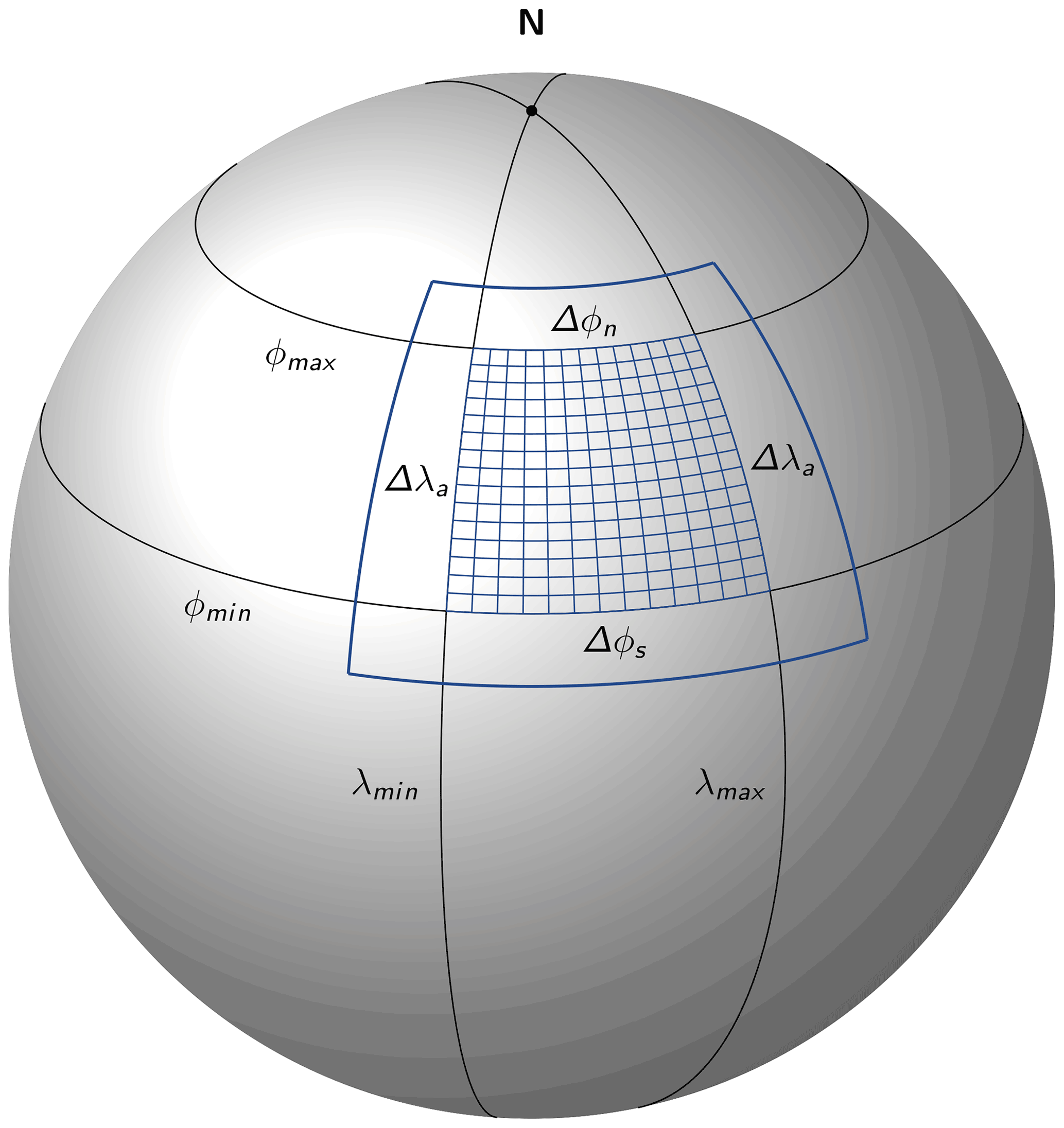
Figure 1Total digital elevation model domain (thick blue line) required to compute the horizon for the inner blue mesh. Black parallels of latitude represent circles and black meridians geodesics.
The required extension in the longitudinal direction can be approximated by
where pl represents the length of the parallel at . This length is computed with
where a represents Earth's equatorial radius (semi-major axis) and e its eccentricity. The total required DEM input domain in the longitude direction is then given by subtracting or adding Δλa from λmin and λmax. The necessary extension in the latitudinal direction (Δϕs and Δϕn) is computed from b via the direct geodesic problem (Karney, 2013), whose equations are implemented in the C++ library GeographicLib and called via a Python wrapper (Karney, 2021). Computing domain extensions is more cumbersome in the case that geographic poles are included.
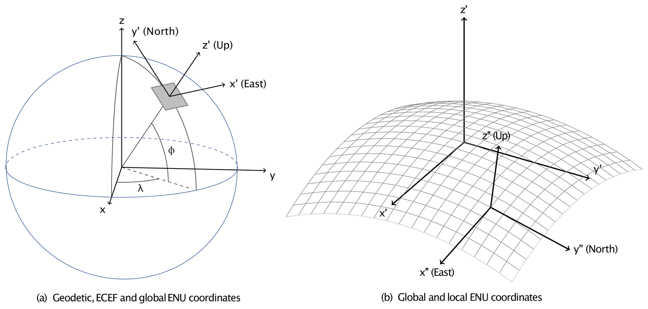
Figure 2Illustration of the different coordinate systems applied: (a) the geodetic coordinate system (λ, ϕ) and the geocentric Earth-centred, Earth-fixed (ECEF) reference system (); (b) the topocentric east–north–up (ENU) reference system () and a second local ENU system (). The grey mesh in panel (b) shows the curvature of the Earth's surface and illustrates how local and global ENU coordinates deviate.
3.1.2 Coordinate transformations and computation of auxiliary quantities
We utilise multiple coordinate systems in this work, which are listed below and partially illustrated in Fig. 2.
-
Map projection (optional)
-
Geodetic coordinates
-
Geocentric Earth-centred, Earth-fixed coordinates (ECEF)
-
Global east–north–up coordinates (global ENU)
-
Local east–north–up coordinates (local ENU)
-
Spherical coordinates in the local ENU reference system
Definitions of these systems and transformations between them are provided in Appendix A. In the case of DEM data on a map projection, we first transform the data to geodesic coordinates. For SwissALTI3D elevation data, we apply the equations provided in Swisstopo (2016). The following steps are then performed identically for all considered DEM products: first, we transform geodetic coordinates to a geocentric Earth-centred, Earth-fixed (ECEF) reference system (). Local up, north and east directions are computed in this coordinate system for every DEM grid cell (see Appendix B1). DEM coordinates and direction vectors are then transformed to a topocentric east–north–up (ENU) reference system (). The origin of these coordinates coincides with the centre of the considered DEM domain, and we refer to this system as global ENU coordinates. The transformation to a global ENU system constrains coordinates to a numerical range that can be represented with sufficient accuracy as single-precision floats. This data type is required in the applied ray-tracing library. The above transformation steps are performed once for a certain DEM domain, and the obtained DEM coordinates and direction vectors in global ENU coordinates are subsequently passed to the ray-casting part of the algorithm. The size of the selected DEM domain is thereby primarily restricted by memory requirements.
Within the ray-casting part of the algorithm (see Sect. 3.2.1), another topocentric reference frame is used – the so-called local ENU coordinate system (x′′, y′′ and z′′). In this reference system, the z axis is always aligned with the local upward direction (and thus the local ellipsoid normal; see Fig. 2b). The same reference system is applied to compute terrain slope aspect and angle (see Appendix B2). This ensures that Eq. (B6) can be solved for any topographic configuration (i.e. the matrix is never singular). Finally, the SVF is computed in a spherical coordinate system, which is referenced to the local ENU system. All above steps regarding coordinate transformations and computations of auxiliary quantities were implemented in Cython (Behnel et al., 2011) and parallelised with OpenMP.
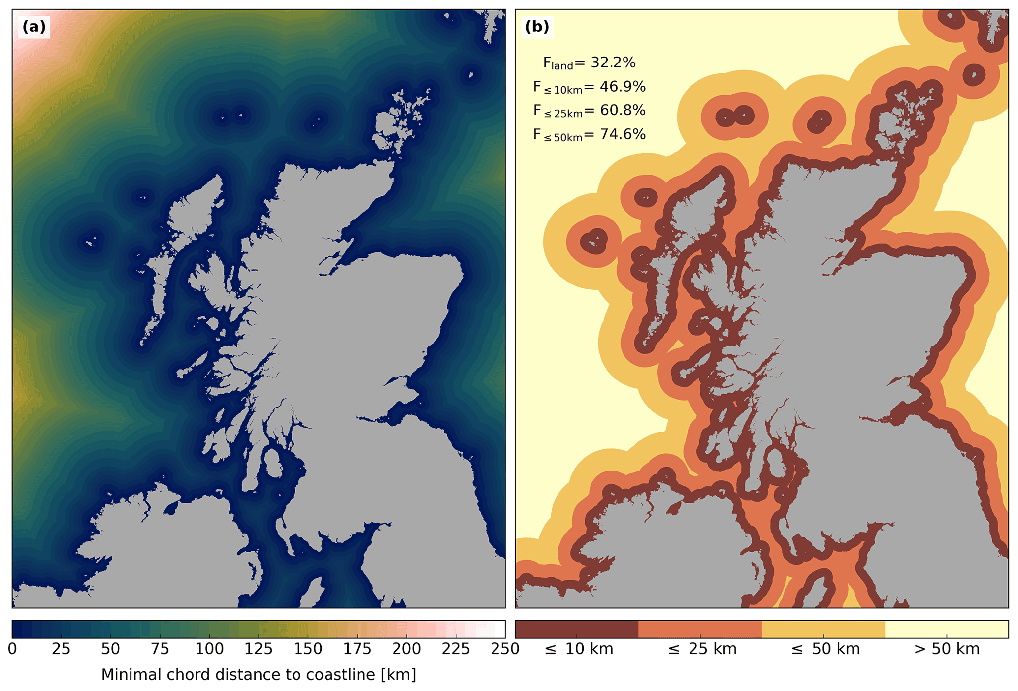
Figure 3NASADEM grid (21 960×32 400 cells) for the northern part of Great Britain and Ireland. (a) Chord distance for every grid cell to the nearest coastline. (b) Ocean grid cells are categorised according to their minimal chord distance to the coastline in bands of ≤ 10, ≤ 25 and ≤ 50 km. The numbers in the upper left indicate the fraction of remaining cells in the case that all ocean cells are masked (Fland) or ocean cells exceeding a certain minimal distance to the coastline are masked.
3.1.3 Masking of ocean grid cells
Computing the horizon from high-resolution elevation data is an expensive operation, even with the method presented in this work. It is thus worthwhile to exclude areas for which horizon information is either not needed or its computation is superfluous due to the non-existence of topography within a relevant radius. The latter applies to a large fraction of ocean grid cells. Unfortunately, such areas are not unambiguously masked in some DEM products. For instance, ocean grid cells in NASADEM have an elevation of 0 m – but inland areas might share the same value. We thus implemented a two-step method to address this issue: first, we label potentially relevant areas in the DEM product (for instance, grid cells with an elevation of 0 m in NASADEM). Subsequently, we rasterise ocean coastlines from the Global Self-consistent, Hierarchical, High-resolution Geography Database (GSHHG; Wessel and Smith, 1996) to the same grid. Grid cells labelled as land in at least one of the two data sets are classified as land, and all remaining cells are treated as ocean. Coastlines are then retrieved from this raster as contour lines. Finally, we have to find the shortest distance to the coastline for every ocean grid cell along a geodesic. This procedure is expensive because an iterative algorithm is required to solve the inverse geodesic problem (Karney, 2013). We therefore use the chord line (the closest straight line connecting two points on the geoid), which can readily be computed in ECEF coordinates. To efficiently find the shortest distance, we transform coastline contours to ECEF coordinates and store them in a SciPy k-d tree (Virtanen et al., 2020). A nearest-neighbour query is then performed for ocean grid cells. Approximating geodesics by chord lines is justifiable because deviations between the two lines are small (e.g. ∼ 1 m for 100 km) for relevant distances. Furthermore, chord lengths are always shorter than geodesics, which guarantees a conservative masking of ocean grid cells.
Figure 3 shows the result of this masking approach for NASADEM data and a region covering the northern part of Great Britain and Ireland. By masking ocean grid cells entirely, horizon information has to be computed for only ∼ 32 % of the total grid cells in the domain. This masking approach might e.g. be useful for land surface models. In the case of considering ocean grid cells and applying a horizon search distance of 25 km, the masking allows excluding ∼39 % of all grid cells in the domain. The implemented masking is not restricted to water grid cells and can be utilised to mask cells based on other criteria (e.g. land surface type, elevation or slope azimuth).
3.2 Computation of horizon by ray casting
3.2.1 General implementation
We perform ray casting with the high-performance ray-tracing library Intel Embree (Wald et al., 2014; Embree, 2021), which has been released as open-source under the Apache 2.0 License. In short, ray tracing in Embree works as follows: first, a BVH is built (in parallel) from input geometries, which can either be based upon triangles, quads (quadrilaterals) or a grid (quadrilaterals on a curvilinear or structured grid). This process recursively wraps the geometries in so-called bounding volumes, which form leaf nodes of a tree. The tree structure allows performing the subsequent ray tracing in a highly optimised way: no children nodes of the tree have to be considered if a ray does not intersect with the parent node. In Cartesian coordinates, DEM data are typically provided on a grid that is (almost) regular, and thus all three Embree geometries can potentially be used. A performance test revealed that ray casting is fastest with quads, while using a grid allows for the fastest BVH building and reveals by far the smallest memory footprint.
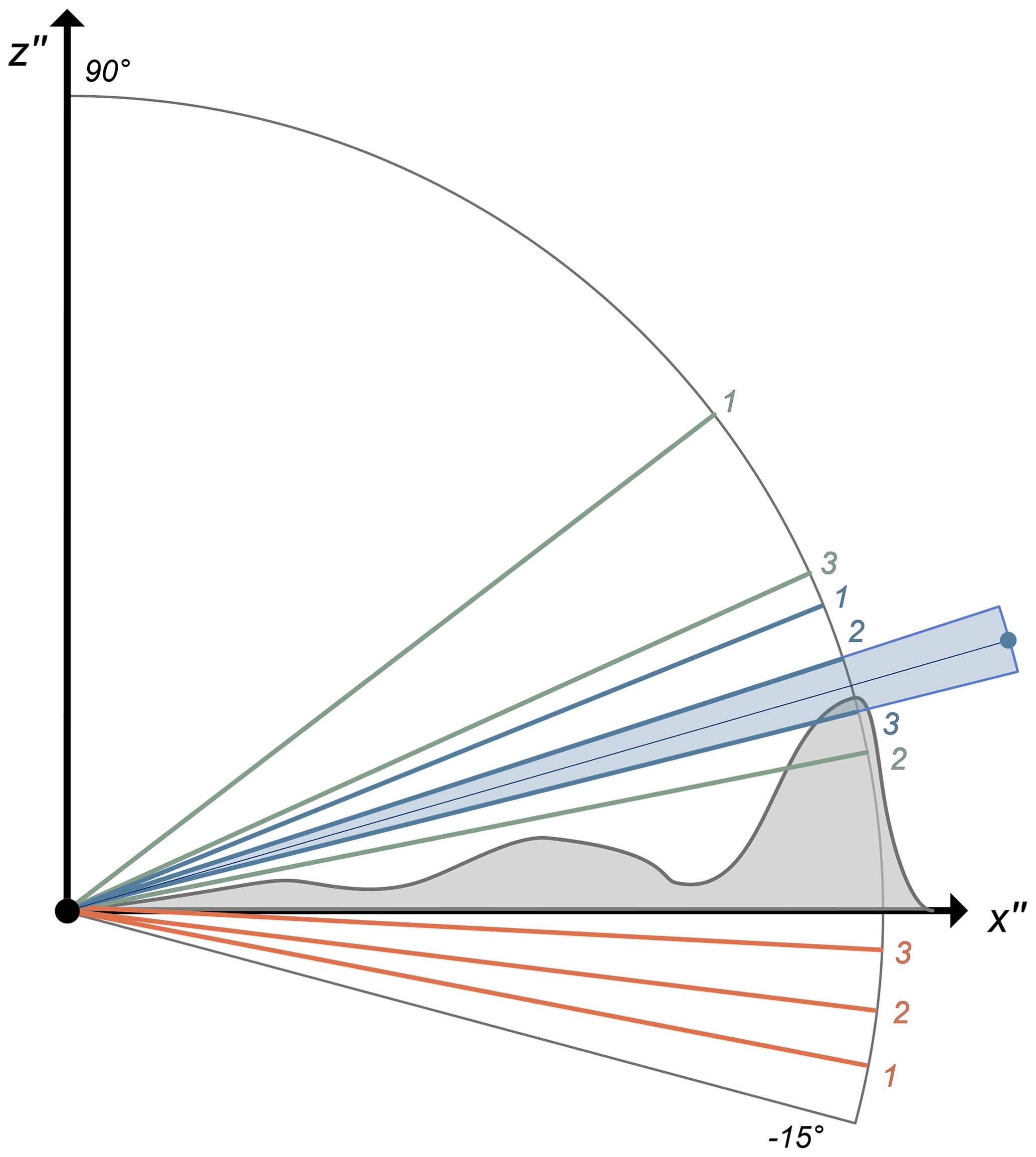
Figure 4Overview of applied horizon detection algorithms with ray casting. Illustrated are the first three rays cast with the methods of discrete sampling (red), binary search (green) and estimating from the previous azimuth (blue). In contrast to the text, an elevation angle spacing of 4∘ is used to allow for better readability. The blue dot marks the horizon estimate from the third method.
In line with other algorithms (Dozier et al., 1981; Dozier and Frew, 1990; Pillot et al., 2016), we compute the horizon for a location by splitting the azimuth angle into discrete sectors and sample along the centrelines. By default, we use 360 sectors. Four different methods were tested to find the horizon within a sector with ray casting (Fig. 4). Because horizon detection results from discrete ray sampling, we have to define a desired accuracy for the horizon (αr), which we set to 0.25∘ by default. The simplest method, called discrete sampling, starts from a minimal elevation angle (−15.0∘ by default) and increments this angle until the ray no longer intersects terrain. The increment Δα is thereby set to 2 αr. The problem can be solved more efficiently by applying a binary search algorithm, which splits the elevation angle range sequentially. The desired accuracy is reached as soon as the difference between the preceding and current ray elevation angle is smaller than 2 αr. Even faster methods can be obtained by considering the fact that the horizon represents a smooth continuous line. Horizon angles between two neighbouring sectors are thus typically very similar, particularly if a high number of azimuth sectors is used. We therefore implemented a third method, which estimates the horizon of the current sector from the previous one. The actual horizon is then found by applying discrete ray sampling from this angle. A fourth method was also tested, which estimates the horizon of the current sector by linear extrapolation from the previous two sectors. However, this method did not result in a speed-up compared to the third method and was thus discarded. For all methods, the actual horizon angle lies within ±0.25∘ of the computed one. By assuming a uniform probability distribution of the actual horizon in the constrained range of the elevation angle (blue shaded area in Fig. 4), the mean error of the computed horizon is ± 0.125∘. To ensure that rays do not intersect terrain directly at their origin due to numerical imprecision, the ray's origin is elevated by a small value of 0.01 m.
The ray-casting part was implemented in C++ and parallelised with Intel Threading Building Blocks (TBB, 2021), which is recommended by Embree and also released under the Apache 2.0 License. In a first implementation, ray directions for a specific location were computed by rotating a vector, which initially points towards local north, in global ENU coordinates. This approach proved to be expensive due to the large number of trigonometric function evaluations. We accelerated this part by storing a discrete number of trigonometric functions, which are needed to compute all necessary ray directions in a local ENU coordinate system. These vectors can subsequently be mapped to global ENU coordinates with Eq. (A5), which is considerably cheaper. Embree offers various options for building the BVH, which affects both BVH building time and subsequent ray casting. An evaluation of these options revealed that for our application, only the flags robust and compact have a significant impact on performance or the memory footprint of the algorithm. The implications of these flags are briefly addressed in Sects. 4.1 and 3.2.2, respectively.
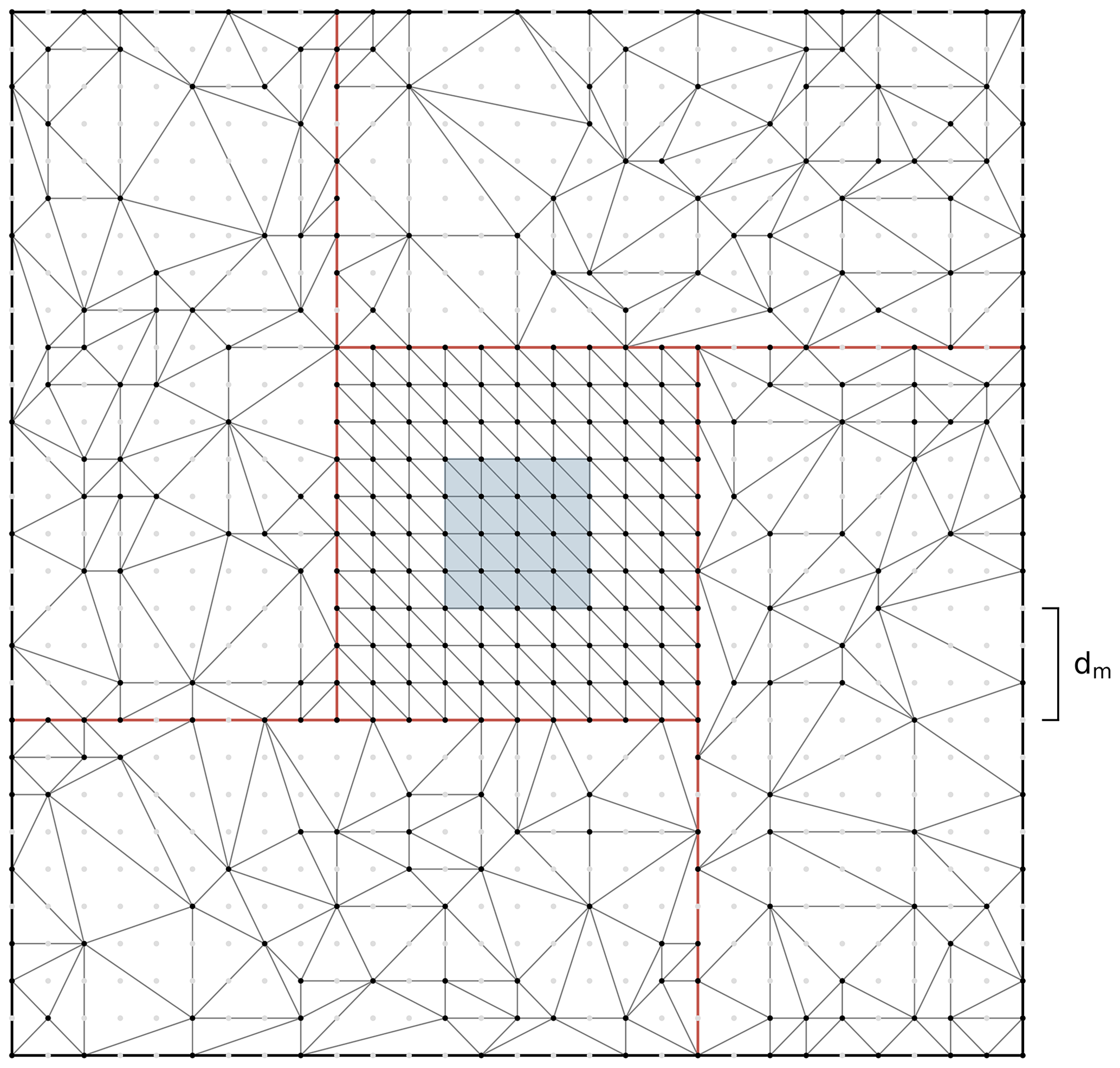
Figure 5Illustration of triangulated surface in the case of terrain simplification in the outer DEM boundary zone. The light grey dots represent grid cell centres of the original DEM data. The blue shaded domain shows the area for which horizon values are computed. Red lines mark discontinuities in the triangulated surface.
3.2.2 Processing of elevation data with very high resolution
A disadvantage of the ray-tracing-based horizon algorithm is its larger memory demand compared to conventional horizon algorithms. Besides the DEM data, which require 3 (x, y and z coordinate) × 4 bytes per grid cell, additional information defining the connectivity of the triangle mesh and the BVH has to be stored. The memory requirements for this auxiliary data are smallest for the input geometry grid and were found to amount to an additional ∼90 % of the space the elevation data occupies. Applying the Embree flag compact did not lower these memory requirements any further (but revealed a significant impact on the memory footprint if quads were used). Currently, various DEMs with very high resolutions are available, like the USGS DEM 1 m (USGS, 2017b), the ArcticDEM (2 m, Porter et al., 2018) and the swissALTI3D, which is available at resolutions of 0.5 and 2 m. In future, further products that cover larger geographical extents will likely become available. Processing such very high-resolution DEM data can result in substantial memory requirements, as shown in the following example: the horizon of a 5×5 km domain should be computed from a 1 m DEM with a horizon search distance of 25 km. The elevation data alone require 36.3 GB of memory without considering space needed for building the BVH. These memory demands exceed the specifications of typical personal computers. However, memory requirements can be drastically reduced by simplifying terrain geometry in the outer boundary zone of the DEM domain (see Fig. 5). We perform this step with the height map meshing utility (hmm; Fogleman, 2021), which simplifies terrain based on a maximal allowed vertical error (Δh). Hmm is based on Garland and Heckbert (1995); it applies a greedy insertion algorithm and subsequent Delaunay triangulation to simplify terrain.
Figure 5 illustrates the setup in the case that terrain simplification is applied. An inner domain, which encompasses the area for which horizon values are computed plus a boundary zone, is represented by the full DEM information. The outer domain is split into four sub-domains, and its terrain geometry is simplified to a triangulated irregular network (TIN). This step can be performed in parallel. Recombination of the five sub-domains introduces discontinuities in the triangulated surface, which are marked by red lines in Fig. 5. These discontinuities have to be patched – otherwise, rays might pass through them without intersection terrain. We perform the patching by adding a vertical strip of triangles (also referred to as skirt; see Fig. 2 in Campos et al., 2020) with a vertical extent of 3Δh. As a consequence of the applied terrain simplification, the accuracy of computed horizon values decreases in the case that the horizon line is located in the outer DEM domain. The horizon accuracy due to terrain simplification αs is thereby linked to the vertical error in terrain Δh by
where dm is the minimal distance between the area for which horizon values are computed and the simplified outer domain (see Fig. 5). This uncertainty in horizon accuracy adds to that from the horizon detection algorithm (αr; see Sect. 3.2.1). Concretely, to e.g. meet a total horizon accuracy of 0.25∘, one could apply the setting αr=0.15∘ and αs=0.1∘.
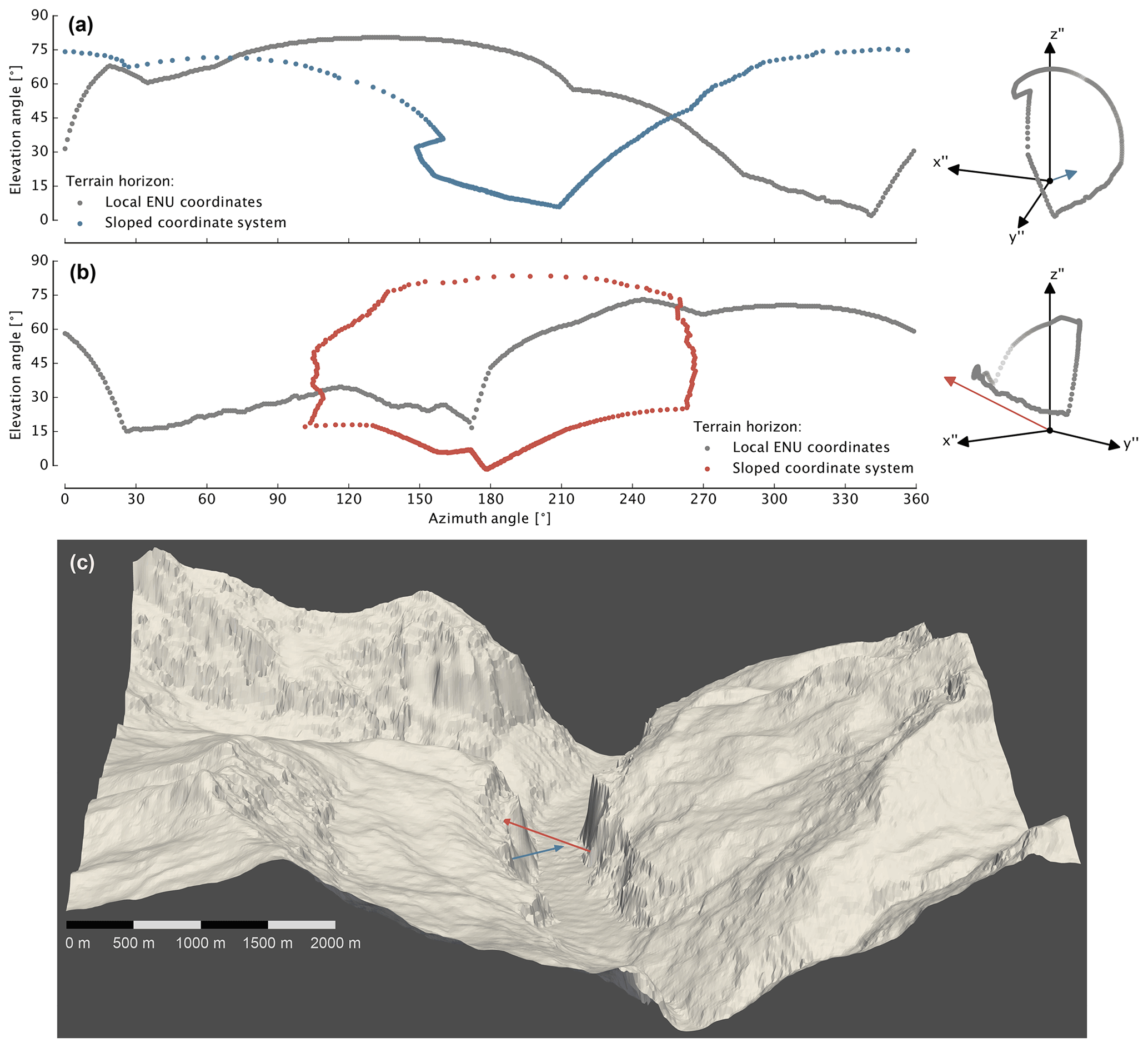
Figure 6Visualisation of the horizon for two locations in the Lauterbunnen Valley (Bernese Oberland, Switzerland). Panels (a) and (b) show the horizon in local ENU coordinates (grey) and in a sloped coordinate system (blue and red, respectively), whose z axis is aligned with the surface normal. Panel (c) illustrates the surrounding terrain of the two locations in an oblique view of the Lauterbunnen Valley from the north. The blue and red arrows represent the surface normals of the two locations. The illustrated domain has an extent of ∼7.5 km (east–west) and ∼6.9 km (north–south). An approximate scale, which is valid for the northern edge of the domain, is provided in the lower left.
3.3 Sky view factor computation
We consider the SVF definition, which yields the fraction of sky irradiance under the assumption of isotropic sky radiation, analogous to Dozier and Frew (1990) and Helbig et al. (2009). For a surface whose normal is parallel to the coordinate system's z axis, the SVF is computed by
with αt representing the elevation angle of the surrounding terrain and ϑ and φ the zenith and azimuth angle, respectively. Integration of Eq. (4) with respect to ϑ yields
This equation is identical to Eq. (8) in Helbig et al. (2009). Equations (4) and (5) are applicable in a sloped coordinate system, in which the surface normal of the terrain aligns with the z axis. An apparently straightforward way to compute Fsky from the horizon, derived according to Sect. 3.2, is to transform horizon angles from the local ENU to sloped coordinates and apply Eq. (5). However, this approach is complicated by several factors: first, it is no longer possible to represent horizon as a function of azimuth in the sloped coordinate system because αt can obtain multiple values for a certain φ (see Fig. 6a). Secondly, if the surface normal intersects surrounding topography due to very steep terrain, then all horizon values are constrained to an azimuth range of 180∘ (Fig. 6b). And finally, the azimuth spacing of transformed horizon angles is no longer regular. Solving the double integral of Eq. (4) in the sloped coordinate system thus requires the consideration of more complex integration limits. Additionally, transformation of all horizon angles to a sloped coordinate system is expensive due to the evaluation of numerous trigonometric functions. We therefore discard this approach and derive an exact SVF equation for horizontal local ENU coordinates.
First, we compute the intersection of the sloped terrain surface with a unit sphere. This plane passes through the origin of the local ENU coordinate system, and thus we can write its implicit plane equation as
with being the surface normal of the terrain in local ENU coordinates. Combining Eqs. (6) and (A7) yields the elevation angle of the plane–sphere intersection αp as a function of the azimuth angle:
A crucial part of the correct SVF equation, which is sometimes omitted in the literature, is Lambert's cosine law, which is represented by cos ϑ in Eq. (4). The angle in this cosine function has to be measured between an arbitrary incoming ray and the surface normal, which is n in the local ENU coordinate system. We can thus express the cosine term as
for local ENU coordinates. Analogous to Eq. (4), we can multiply the cosine term with the surface element of a sphere (sin ϑ dϑ dφ) and integrate with respect to φ and ϑ, which yields
where is either defined by the surrounding terrain horizon or the local (sloped) surface. Integration of Eq. (9) with respect to ϑ yields
This represents the analytical formulation of the SVF. To apply this equation with computed terrain horizon angles, we have to discretise it to
where M represents the number of equally spaced azimuth directions for which the horizon was computed. In principle, one could improve the accuracy of the numerical integration by employing Simpson's rule; however, we believe that the overall uncertainty is not determined by the errors of this integration, but rather by the computational resolution of the horizon computation.
In the literature, SVF computation is performed with different methods, which are, for instance, based on formulations from Helbig et al. (2009), Manners et al. (2012), and Dozier and Frew (1990). Computing the SVF in a sloped coordinate system with the equation suggested in Helbig et al. (2009), which is identical to Eq. (5), requires careful consideration of the integration limits. As illustrated by the blue and red dots in Fig. 6a and b and as previously discussed, these limits can be complicated for steep and complex terrain. Integration can be performed successfully with the trapezoidal rule and by summing up obtained areas – analogous to the area computation of a two-dimensional polygon. Apart from negligible numerical deviations, we obtained the same results with this method compared to applying Eq. (11). By testing the method of Manners et al. (2012), we believe we have found an error in its derivation: in Eq. (13) of Manners et al. (2012), angles are added that are expressed in different coordinate systems. The resulting error is minor for small slope angles but more pronounced for steeper terrain. Finally, we considered the method suggested by Dozier and Frew (1990). By applying multiple trigonometric identities and considering the different coordinate systems applied, we found it to be identical to our solution. Concluding, if horizon angles are available in a horizontal coordinate system, it seems most convenient to perform the SVF integration in the same reference system.
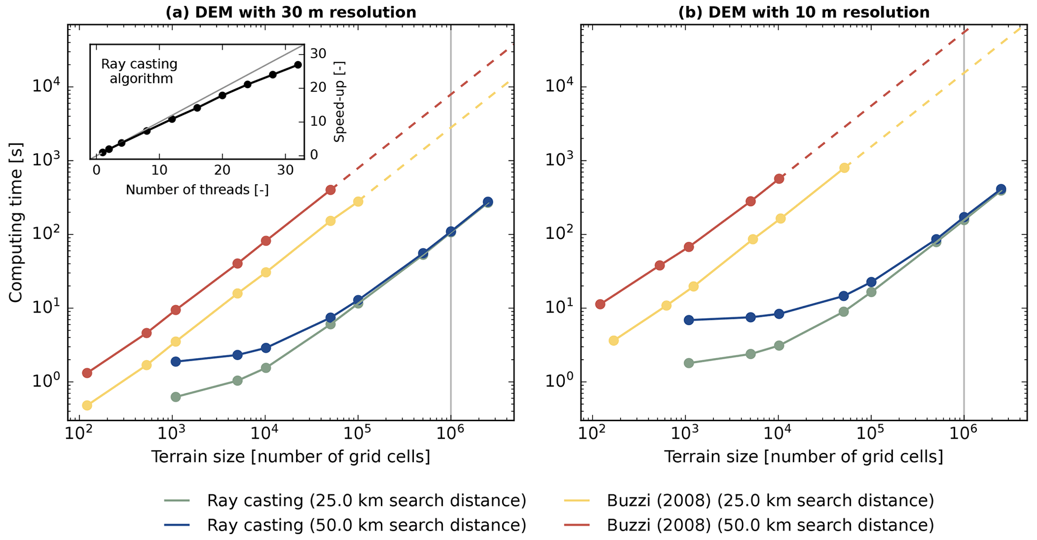
Figure 7Computational performance of the ray-casting algorithm relative to the one implemented by Buzzi (2008) in a log–log plot. Panels (a) and (b) show the performance for a DEM with 30 and 10 m horizontal resolution, respectively. Dashed lines indicate a linear extrapolation of the performance relationship. The inset panel in (a) shows the parallel scaling performance of the ray-casting algorithm for a fixed terrain size of approximately 106 grid cells, a horizon search distance of 50 km and a DEM resolution of 30 m.
We consider two reference horizon algorithms to evaluate the computational performance and accuracy of our method: the first is the algorithm described in Pillot et al. (2016), which is available as a MATLAB implementation (Pillot, 2016). The second is the algorithm applied in Buzzi (2008), which was implemented in the pre-processing tool of the limited-area atmospheric model COSMO (Steppeler et al., 2003) in Fortran and parallelised with OpenMP. Both algorithms are based on the conventional concept of sampling all elevation data along a centreline of an azimuth sector. The algorithm by Buzzi (2008) was developed to process elevation data on a rotated latitude–longitude grid centred at the coordinate system's origin. The Earth's shape is furthermore assumed to be spherical. Due to these restrictions, we processed the input DEM data for this section as follows: first, we assume that DEM heights are referenced to a spherical Earth and ignore differences between orthometric and ellipsoidal heights. Secondly, we bilinearly remapped DEM data to rotated longitude–latitude coordinates, whose origin is located in the centre of the selected DEM domains. We apply two elevation data sets in this section: NASADEM, with a horizontal resolution of 30 m, and the USGS arcsec DEM, which has a higher horizontal resolution of 10 m. For all algorithms, we used the default number of 360 azimuth sampling sectors. For the ray-casting-based algorithm, the elevation angle accuracy was set to ±0.25∘ and terrain simplifications according to Sect. 3.2.2 were not applied.
4.1 Evaluation of the computational performance
In the literature, suggested search distances for the horizon typically range from ca. 20 km (Senkova et al., 2007) to 50 km (Dürr and Zelenka, 2009). These distances should be defined according to the desired horizon accuracy and the complexity of the regional terrain. In areas like the Himalayas, elevation differences within 50 km can be as high as 7000 m (without intermediate terrain obstruction), which corresponds to a horizon angle of ∼ 8∘. For such terrains, a search distance even larger than 50 km might be necessary if high horizon accuracy is required. We applied NASADEM data, centred at Kleine Scheidegg (Bernese Oberland, Switzerland), and USGS arcsec DEM data, centred at Denali (Alaska, USA), for the performance evaluation. The performance analysis of the ray-tracing-based method revealed a dependency on terrain complexity, and the algorithm's performance is higher for simpler terrain. We therefore considered two additional domains for this algorithm, which are located north of the above-mentioned domains and feature less complex, hilly terrain. The overall performance was then computed as an average between the two domains with different terrain complexity. The performance dependency on terrain, however, is minor and of the order of ±10 % from the average. Performance experiments have been carried out on a workstation with an Intel Core i5 Quad-Core processor (3.4 GHz) with 16 GB of memory, except for assessing the parallel scaling performance of the algorithm, which was evaluated on an Intel Xeon Gold processor (3.4 GHz) with 2×16 physical cores and 1.5 TB of memory.
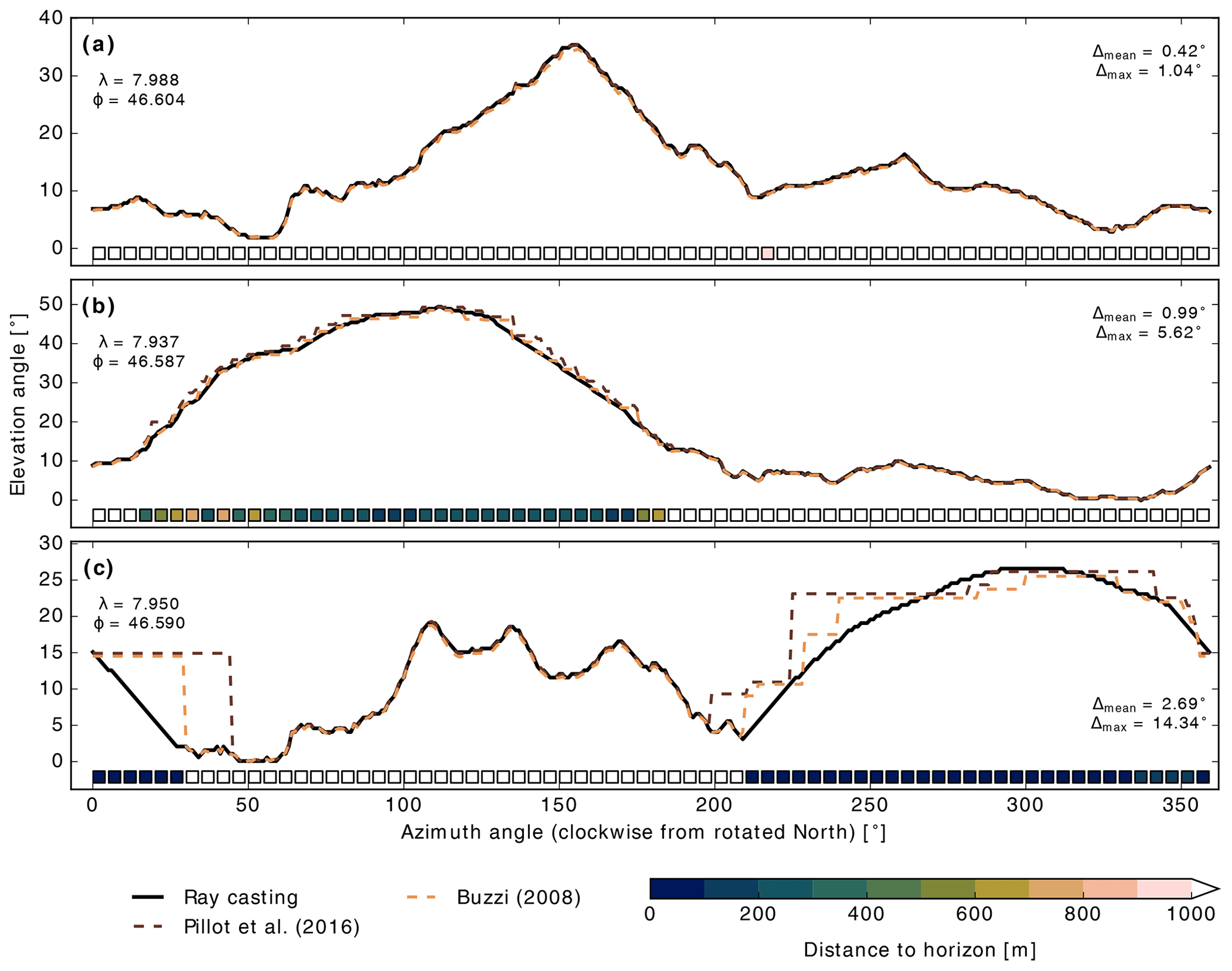
Figure 8Horizons for three locations computed with the three different algorithms. The boxes at the lower boundary of the panels illustrate the distance to the horizon line based on the ray-casting algorithm. The numbers in the panel's upper left show the geographic longitude (λ) and latitude (ϕ) of the location. The numbers at the right boundaries of the panels represent the mean (Δmean) and maximal (Δmax) spread in computed horizon angles for the location. The three methodologies considered qualitatively agree, but note the occurrence of staircase-like behaviour for the Pillot and Buzzi algorithms.
Figure 7 shows results from the performance analysis for two different horizontal DEM resolutions and horizon search distances. The algorithm of Pillot et al. (2016) is not considered in this analysis because it was designed for point location applications (its run time is substantially larger than the other two considered algorithms). Figure 7a reveals that the run time of the conventional algorithm (Buzzi, 2008) scales distinctively with horizon search distance. For the ray-tracing-based method, this is only true for relatively small (ca. <105 grid cells) terrain sizes. This diverging pattern is caused by the varying ratio of time spent on BVH building and ray tracing. For small domains, the BVH building contributes significantly to the total run time, whereas for larger domains, this contribution is negligible. For larger domains (ca. >105 grid cells), run times for the ray-casting algorithm are almost independent of the horizon search distance. For the DEM with 10 m resolution (Fig. 7b), the performance analysis looks overall very similar. However, run times between the conventional and the ray-tracing-based algorithm diverge even further: for processing 106 grid cells with a search distance of 50 km, the new algorithm reveals a speed-up factor of ∼ 72 for a 30 m DEM, whereas this factor increases to ∼ 321 for a 10 m DEM. As mentioned in Sect. 3.2.1, Embree offers an option for robust BVH building, which we used for the analysis shown in Fig. 7. Disabling this option increases ray-tracing performance by approximately 20 %. However, as a trade-off, the requirements for horizon accuracy are no longer strictly met because triangles from the terrain mesh might be missed by rays. We thus always enable the flag robust for BVH building, even if such errors were found to occur extremely infrequent. The inset panel in Fig. 7a shows the parallel scaling performance of the ray-casting-based horizon algorithm. For the considered terrain size and setup, the algorithm reveals excellent scalability with a speed-up factor of ∼27 using 32 cores relative to a single-core execution.
In summary, the performance analysis revealed that the ray-casting method is much faster for all considered terrain sizes (by about 2 orders of magnitude). The speed-up increases with both higher spatial DEM resolution and larger horizon search distances as well as with terrain size up to approximately 106 grid cells. The higher performance of the ray-tracing-based algorithm is mainly caused by the more efficient storage of DEM data, which drastically reduces the elevation information that has to be considered along a sampling line. The relevance of this effect grows with both increased DEM resolution and horizon search distance.

Figure 9Terrain parameters for the two idealised geometries Crater (blue) and Crater hill (red). (a) Elevation cross-sections of the two terrains; black symbols mark locations for which the horizon is illustrated in (b) and (d). In (b), exact solutions (grey lines) for the horizon are shown in addition to the ones computed with ray casting. Panels (c) and (e) illustrate horizontally resolved SVF for the Crater and Crater hill geometries; the black symbols again indicate the locations considered in (b) and (d).
4.2 Accuracy evaluation for real terrain
We compared the accuracy of the ray-tracing-based horizon algorithm to the methods suggested by Buzzi (2008) and Pillot et al. (2016). The accuracy of the latter algorithm was assessed by in situ horizon measurements collected with a theodolite in Corsica (Pillot et al., 2016). We evaluated the different algorithms for an approximately 10 by 10 km wide NASADEM domain (324×324 grid cells) centred at Kleine Scheidegg (Bernese Oberland, Switzerland). To increase overall accuracy of the computed horizon lines, we enhanced the search distance for the horizon to 100 km. Due to the comparably high run time of the Pillot et al. (2016) algorithm, we did not apply it to the full domain. Instead, we ran it for 1000 cells within the 324×324 domain, which were drawn by random uniform sampling.
Figure 8 shows obtained horizon lines for three example locations. In Fig. 8a, the distance to locations forming the horizon is generally larger than 1 km, and the agreement between the three algorithms is, with a mean spread of 0.42∘, very good. For locations shown in Fig. 8b and c, the agreement between the algorithms deteriorates and maximal deviations up to 14.34∘ occur. Considering the horizon distance information, it is obvious that the inferior agreement is constrained to azimuth angles with distances close to the horizon. For these ranges, both reference algorithms indicate staircase-shaped changes in the horizon line, which is e.g. also apparent in Fig. 9 in Pillot et al. (2016). Table 1 indicates that findings from the three example locations translate to the entirety of analysed locations. The agreement between the three algorithms is considerably smaller for locations and azimuths with close (<1 km) proximity to the horizon line – in terms of both statistical mean and 95th percentile. Additionally, Table 1 reveals that the agreement between the ray-casting and Buzzi (2008) algorithm is consistently better than between the other two combinations. Deviations from the algorithm by Pillot et al. (2016) are higher for large horizon distances. A potential explanation for this pattern might be the way sampling for a certain azimuth direction is implemented in Pillot et al. (2016), which happens along a loxodrome.
Table 1Absolute differences in horizon angles [∘] between the three algorithms. The mean and the 95th percentile (p95) are shown for all data and grouped according to the associated distance to the horizon.

The pronounced staircase-shaped artefacts in Fig. 8b and c, which cause the poor agreement between the algorithms for close horizon distances in Table 1, are induced by the non-smooth terrain representation in the reference algorithms of Buzzi (2008) and Pillot et al. (2016). These algorithms assume uniform elevations within grid cells with vertical drops at the cells' edges. The non-smooth terrain representation introduces two disadvantages: the first is the occurrence of unnatural steps in the horizon line (see Fig. 8c), and the second is high sensitivity of the computed horizon to the chosen azimuth angle. The relevance of these issues increases with decreasing distance between the centre location and the horizon. If computed horizon lines are used for SVF calculations, the issue of artificial steps is partially attenuated because terrain horizon αt is occasionally exceeded by plane horizon αp and thus not considered (see Sect. 3.3). However, some of the error does propagate to computed SVF values. In the ray-casting algorithm, gridded DEM data are converted to a triangle mesh, which represents a smooth surface. Subsequently, this algorithm does not suffer from the aforementioned issues.
4.3 Verification with idealised terrain geometries
To quantitatively verify our methodology, we additionally assessed the implemented horizon and SVF algorithms by means of two idealised z-axis-symmetric terrain geometries. The first one, called Crater, represents a simple hemispherical cavity, which was also considered in Manners et al. (2012). Its elevation h is defined according to
where d is the distance from the centre and r the radius of the cavity. Except for the rim of the cavity, the terrain represented by this geometry is concave, which implies that horizon lines are almost exclusively formed by non-adjacent terrain. To cover the other case, we consider a second, partially convex geometry (Crater hill), whose elevation is defined by
where fa represents the amplitude factor, which determines the height of the central bump. Cross-sections of the two geometries are shown in Fig. 9a for the parameter setting r=1000 m and fa=0.9.
We discretised both terrains by 1026×1026 grid cells and computed the horizon with the default setting of 360 azimuth sectors and an accuracy of 0.25∘. The resulting horizon for three grid cells, whose location is marked in Fig. 9a, is illustrated in panels (b) (Crater) and (d) (Crater hill) of the same figure. In accordance with the smooth surfaces of the geometries, horizon angles represent smooth lines without artefacts. In the case of the Crater geometry, the horizon is invariably formed by the rim of the cavity and its exact solution can thus readily be derived. Figure 9b indicates that horizon lines computed with ray casting align with these “perfect” solutions. Obtained spatial SVF values for both geometries are shown in Fig. 9c and e. The SVF for the Crater geometry is uniformly 0.5 within the cavity (with negligible numerical deviations), which is in line with the analytical solution derived in Manners et al. (2012). The SVF for the Crater hill geometry is spatially variable with the lowest values around and the highest values in the centre.
It is possible to validate the resulting SVF values of both geometries, at least in a horizontally aggregated way, by physical and geometrical considerations: Manners et al. (2012) illustrate in Sect. 2.4 that the same horizontally aggregated longwave flux is emitted from a flat disc and a hemispherical cavity. This relation holds for any cavity – not only the perfectly hemispherical one. We can rearrange Eqs. (24) and (25) of Manners et al. (2012) to
where Acavity and Adisc represent the surface area of the cavity and the flat disc, and Fsky, disc represents the SVF of the disc, which is exactly 1. Applying Eq. (14) to the Crater and Crater hill geometries yields ∼0.999 for both cases, which confirms the correct implementation of the horizon and SVF algorithm.
In this section, we present example applications of the ray-tracing-based horizon and SVF algorithm. Output from Sect. 5.1 and 5.2 can be used to parameterise the effect of terrain on surface radiation in weather and climate models. Section 5.3 illustrates the computation of horizon and SVF from very high-resolution elevation data. These outputs are primarily interesting for very high-resolution land surface models applied in mountainous terrains.
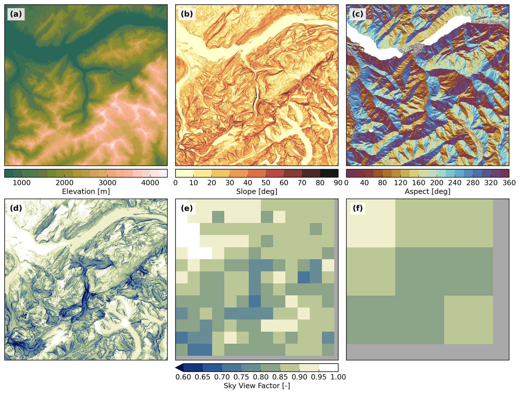
Figure 10Terrain parameters computed from NASADEM for a 40 km wide window centred at Lauterbunnen Valley (Bernese Oberland, Switzerland). Panels (a) to (c) illustrate the elevation, slope angle and slope aspect. Note that aspects with slopes are masked. Panel (d) shows the computed SVF at the native resolution of ∼30 m and panels (e) and (f) the spatial aggregation of this parameter to 3 and 12 km, respectively.
5.1 Computation of terrain parameters and sub-grid sky view factor
As mentioned in the Introduction, terrain parameters like horizon and SVF are already applied in several numerical weather and climate models to account for topographic effects on radiation. In some models, terrain parameters are derived from the model's internal elevation representation, which typically features grid spacings of >500 m to ∼ 100 km. This elevation data are normally smoothed to ensure numerical stability of the model. The relatively coarse spacing (and the potential smoothing of orography) leads to a smoothing of terrain parameters – i.e. computed horizons angles are typically lower and obtained SVF values higher. In other models, terrain parameters are computed from a sub-grid-scale DEM and subsequently spatially aggregated. In the latter case, DEM data with high spatial resolution have to be processed, which can be done efficiently with our ray-tracing-based algorithm. Such a sub-grid-scale parameterisation is, for instance, presented in Helbig and Löwe (2012), which emulates the effects of terrain reflection of shortwave radiation on surface albedo.
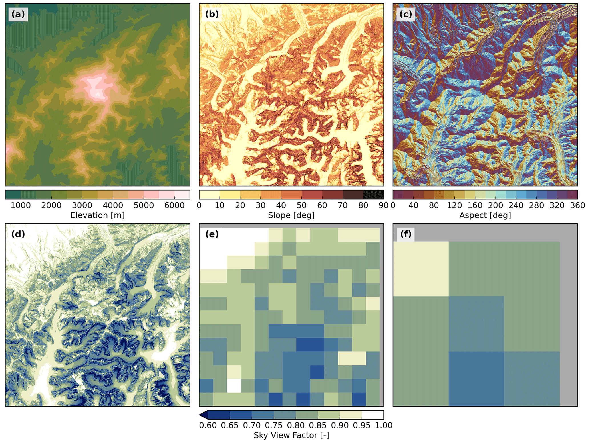
Figure 11Terrain parameters computed from the USGS arcsec DEM for a 40 km wide window centred at Denali (Alaska, USA). Panels (a) to (c) illustrate the elevation, slope angle and slope aspect. Note that aspects with slopes are masked. Panel (d) shows the computed SVF at the native resolution of ∼10 m and panels (e) and (f) the spatial aggregation of this parameter to 3 and 12 km, respectively.
We illustrate the computation of terrain parameters and the spatial aggregation of the SVF by means of two DEMs with different resolution, the NASADEM and the USGS arcsec DEM. Output from the NASADEM is shown in Fig. 10 for a 40 km wide domain centred at Lauterbunnen Valley (Bernese Oberland, Switzerland). The horizon was computed with the default setting of 360 azimuth sectors and a search distance for the horizon of 50 km. Panels (d) to (f) illustrate how the range of SVF changes with spatial aggregation. Common horizontal resolutions applied in regional climate modelling are 3 and 12 km (Ban et al., 2021; Sørland et al., 2021; Jacob et al., 2014). Figure 10f shows that, even at a relatively coarse resolution of 12 km, the aggregated SVF of some grid cells is still significantly smaller than 1.0. Figure 11 illustrates terrain parameters computed from the USGS arcsec DEM for a 40 km wide area centred at Denali (Alaska, USA). The geographic latitude of this area is relatively high (N), which means that topographic shading is a very relevant process due to low solar elevation angles – particularly during Northern Hemisphere winter. In contrast to NASADEM processing, the number of azimuth sectors was decreased to 60 to reduce the required storage space for the three-dimensional horizon information. Compared to Fig. 10, obtained SVF values on the native grid are generally lower. This translates to the spatially aggregated SVF values, and even on a scale of 12 km, almost the entire area features SVF values below 0.85 (see Fig. 11f).
Table 2Different geographic domains used to test the accelerated computation of sub-grid SVF values.
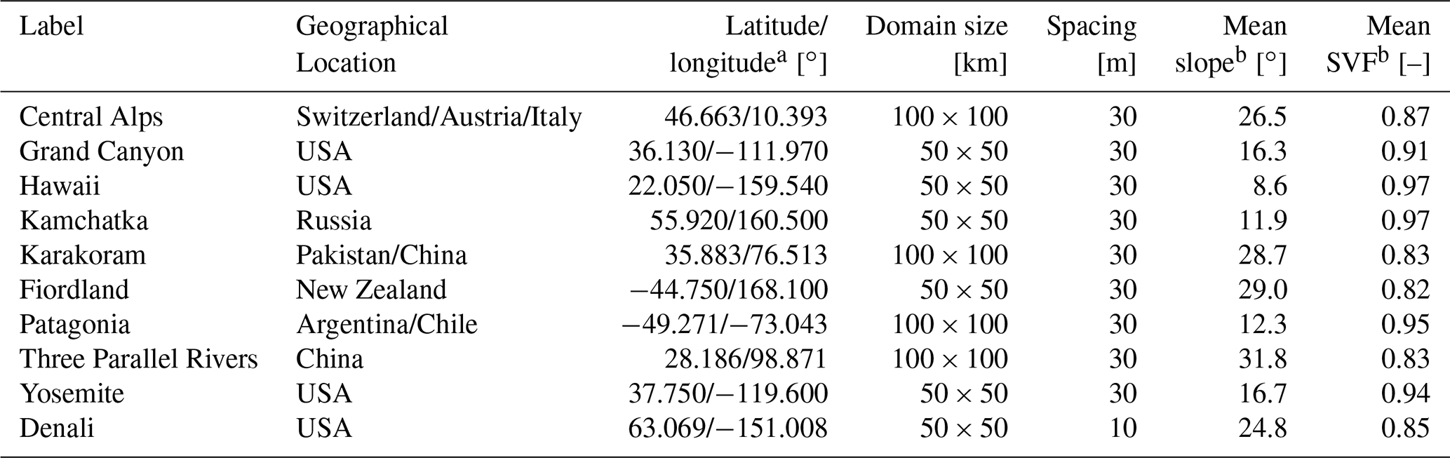
a Geographic coordinates refer to the centre of the domain. b Computed with the reference sampling density (∼ 1024 samples per km2).
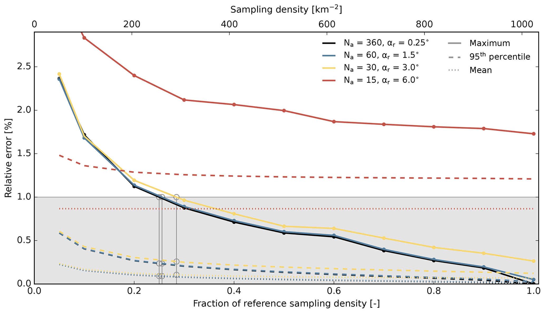
Figure 12Example of the relative error in spatially aggregated SVF for the Central Alps region as a function of sampling density. The figure displays errors from 104 randomly and spatially uniformly drawn samples for an aggregation to 3 km. Na denotes the number of applied azimuth sectors and αr the horizon accuracy. The lower x axis shows the sampling density relative to the reference density (∼1024 samples per km2), while the upper x axis indicates absolute values. Intersections of the coloured solid lines, which represent the maximal relative error, with the horizontal 1 % error line are denoted by grey circles and vertical lines.
5.2 Accelerated computation of sub-grid sky view factor
The application of sub-grid SVF in weather and climate models, such as in Hao et al. (2021), requires the computation of high-resolution horizon for large domains spanning several hundred to several thousand kilometres. This step is computationally expensive, even with the new horizon algorithm (with the default setting of Na=360 and αr=0.25∘) presented in this study. We thus tested two approaches to decrease computational time further while maintaining a high level of accuracy: on the one hand, we decreased the number of azimuth sectors and the horizon accuracy. These two parameters are interdependent in the fastest horizon detection method (see Sect. 3.2.1). If e.g. only Na is decreased, the average number of rays applied per sampling location and sector increases due to larger horizon differences between neighbouring sectors. We thus only considered settings in which both Na and αr are altered simultaneously to keep the averaged number of rays per grid cell and sector similar. We considered three combinations beside the default setting: Na=60 and αr=1.5∘, Na=30 and αr=3.0∘, and Na=15 and αr=6.0∘, which represent performance increase factors of ∼ 6, ∼ 12 and ∼ 24. On the other hand, we reduced spatial sampling density. For this analysis, we bilinearly remapped NASADEM and USGS arcsec data to resolutions of ∼ 31.3 and ∼ 10.4 m, respectively. This allows for a simple spatial aggregation of sub-grid SVFs to grids with resolutions of 1 km and integer multiples, as a 1 km2 cell contains exactly 32×32 (NASADEM) or 96×96 (USGS arcsec DEM) resampled DEM cells. For the reference solution, we consider SVF information from all NASADEM sub-grid cells and of all USGS arcsec DEM sub-grid cells, which corresponds to a spatial sampling density of ∼1024 times per km2. Subsequently, we decreased spatial sampling densities by considering subsets of the reference sampling locations, which were drawn randomly and spatially uniformly. To obtain more robust results, we repeated the random drawing 104 times. We performed these tests for 10 different geographic domains, which cover a broad range of geomorphologies (see Table 2). Spatial SVF aggregation scales of 1, 3, 12 and 25 km are considered, which represent common horizontal resolutions for numerical weather and climate models.
Figure 12 illustrates the obtained results for the Central Alps region and a spatial aggregation of the sub-grid SVF values to 3 km. As expected, decreasing sampling density induces a gradual increase in relative SVF error in all considered error statistics (maximum, 95th percentile and mean). Remarkably, this gradual behaviour is less evident for the applied sets of Na and αr. Initial decreases in Na, until Na=30, revealed minor effects on the accuracy of the computed sub-grid SVF. Only the decrease from Na=30 to Na=15 showed a clear deterioration in the accuracy of sub-grid SVF. The same behaviour was also found for other geographical regions. The grey circles and vertical lines in Fig. 12 illustrate the required sampling density to meet a maximal relative error of 1 % and the associated 95th percentile and mean of this error.
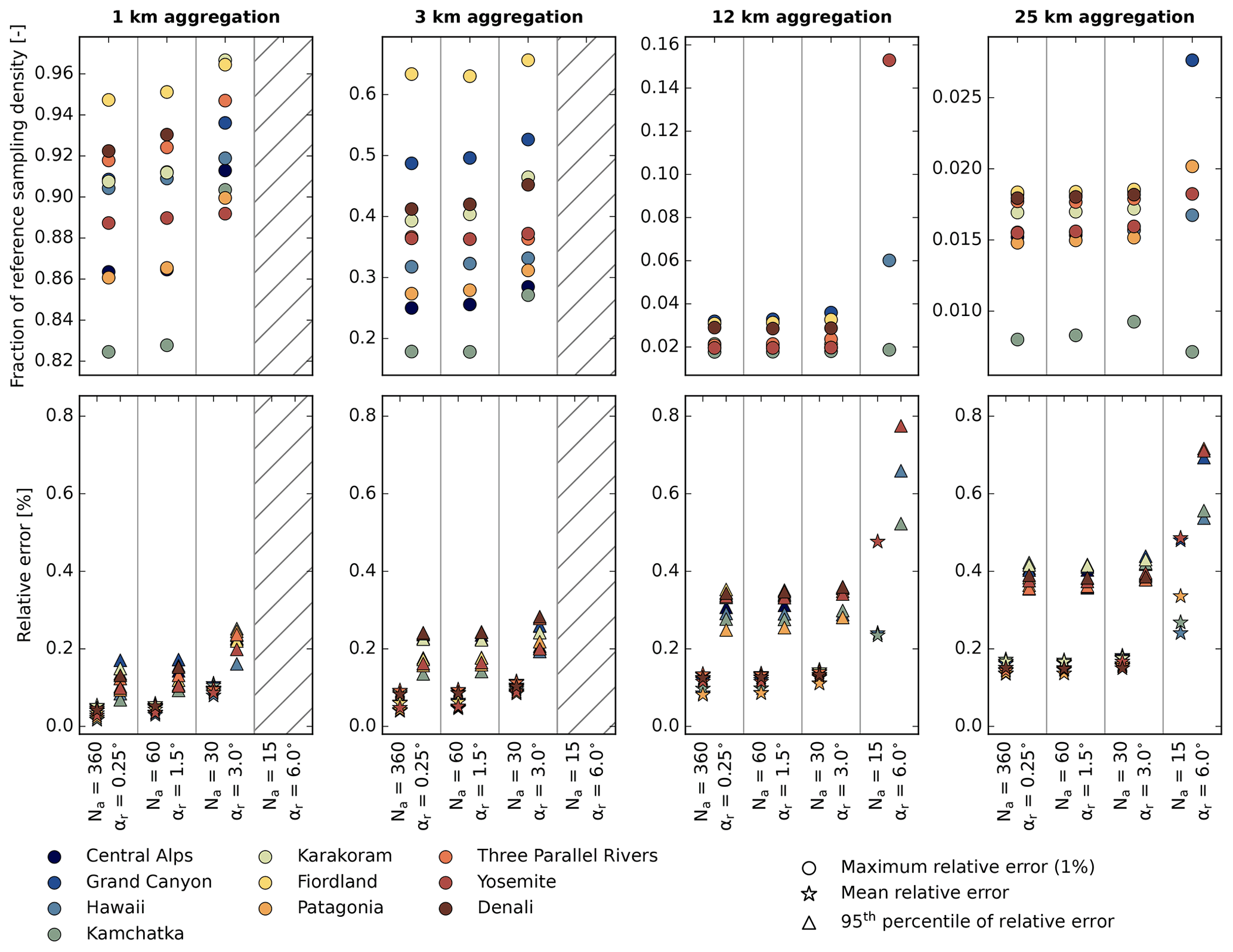
Figure 13Overview of error statistics for the applied speed-up tests of sub-grid SVF calculation. The upper row illustrates the required spatial sampling density to meet a maximum relative error of 1 % in sub-grid SVF computation. The lower row shows the associated 95th percentiles and means in relative error. Settings (Na and αr) for which the maximum relative error never falls below 1 % are hatched. Note the variable y-axis range between panels in the upper row.
Figure 13 displays these values for all considered regions and spatial aggregation scales. Values for different regions are typically clustered in relatively narrow bands. Apparently, the Fiordland region in New Zealand exhibits the highest terrain complexity, as it typically requires the highest sampling density to meet the 1 % maximum relative error (see upper row in Fig. 13). In contrast, the Kamchatka region in Russia requires a comparably low sampling density. This can be explained by the relatively simple terrain geometry of this region, which is shaped by stratovolcanos. For all conducted experiments, the 95th percentile and the mean in relative error remain below 0.5 % and 0.2 % – except for the experiment with Na=15 (see lower row in Fig. 13). Regarding speed-up factors for computing sub-grid SVF with a maximal absolute error of 1 %, the following conclusions can be drawn from Fig. 13: for a spatial aggregation to 1 and 3 km, the setting Na=30 and αr=3.0∘ is most favourable, while a decrease in the spatial sampling density is not (or only to a minor extent) possible. This allows a performance increase relative to the default setting of a factor of ∼ 12. For the spatial aggregation to coarser resolutions (12 and 25 km), the setting Na=30 and αr=3.0∘ is again optimal. For these resolutions, the sampling density can additionally be reduced to 5 % (12 km) and 2.5 % (25 km) of the reference density. This yields total speed-up factors of ∼240 () and ∼480 () for sub-grid SVF computations for resolutions of 12.0 and 25.0 km, respectively.
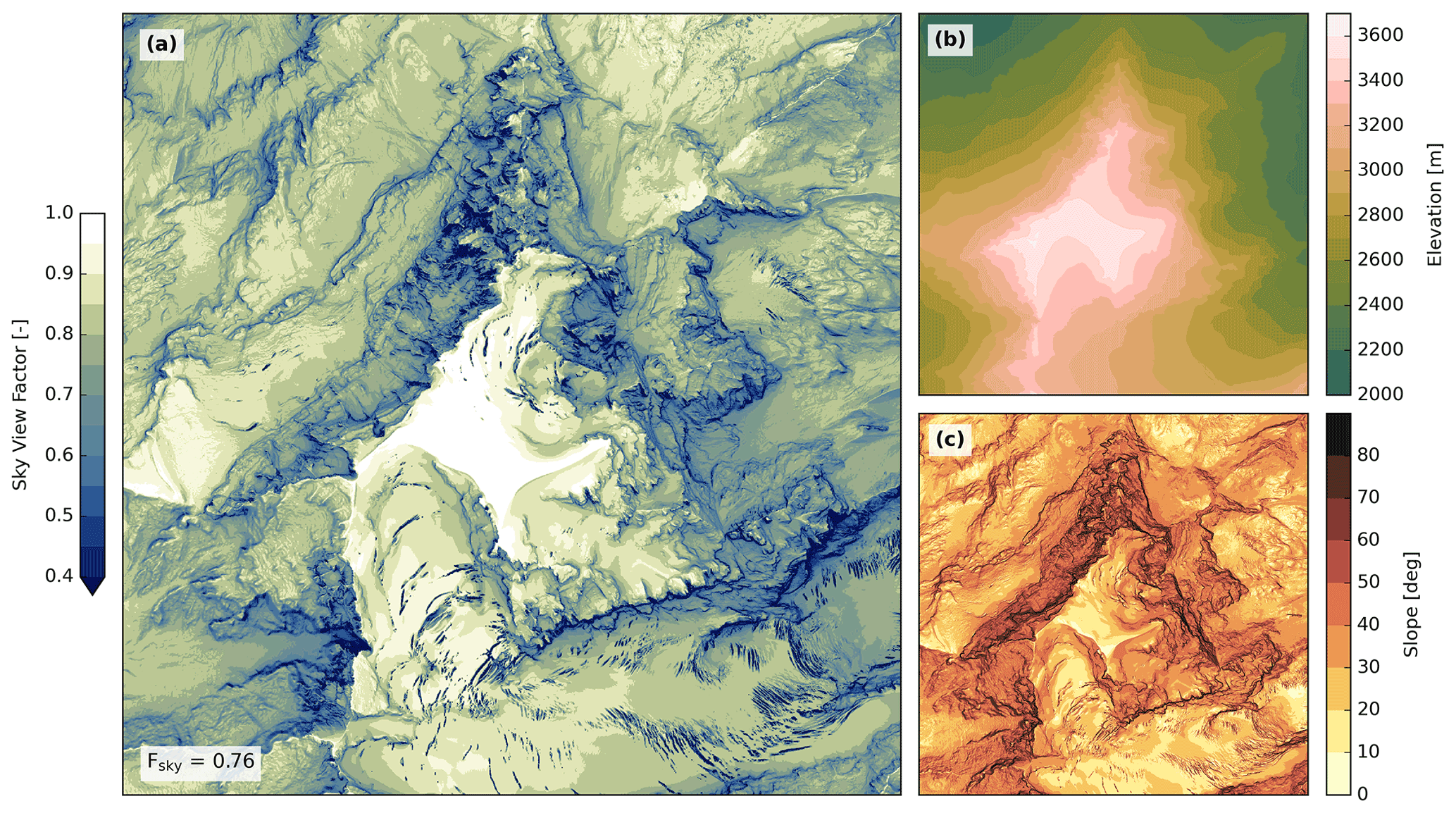
Figure 14Terrain parameters computed from the 2 m SwissALTI3D DEM for a 3 km wide domain centred at Tödi (Glarus Alps, Switzerland). Panel (a) illustrates the spatially gridded SVF, while the number in the lower left represents the domain-wide average. Panels (b) and (c) show the associated surface elevation and slope angles.
An earlier method to compute sub-grid-scale SVF was presented in Helbig and Löwe (2014). They developed a model that estimates spatially aggregated SVF from local terrain parameters, which are cheap to compute. This model is faster than our approach but also exhibits larger relative errors in computed SVF – particularly for target grids with high spatial resolutions (1.0–2.5 km). The choice of model, i.e. Helbig and Löwe (2014) versus our approach, depends on the available computational resources and the desired accuracy for the sub-grid-scale SVF. An advantage of our approach is its potential to seamless derive accurate sub-grid SVF values for all spatial scales.
5.3 Application to very high-resolution DEM data
In this section, we demonstrate the application of the horizon and SVF algorithm with very high-resolution DEM data. As mentioned in Sect. 2, we used SwissALTI3D data with a horizontal resolution of 2 m. To lower the memory footprint of the high-resolution data during processing, we simplified terrain representation in the boundary zone of the DEM according to Sect. 3.2.2. We computed terrain parameters for two 3×3 km domains in the Glarus Alps in Switzerland.
The first domain is centred around Tödi and is overall convex-shaped (Fig. 14), while the latter is centred at Limmerensee and features a rather concave-shaped terrain geometry (Fig. 15). For the absolute horizon accuracy, we selected a value of 0.25∘, which is partitioned to αr=0.15∘ and αs=0.1∘. For dm (see Fig. 5), we chose a distance of 7 km. For the domain centred around Tödi, a search distance for the horizon of 30 km was applied. Choosing a larger distance is not possible due to the limited spatial coverage of SwissALTI3D data. Without terrain simplification, the memory footprint of the DEM data amounts to ∼11.9 GB, while with terrain simplification, total memory requirements can be lowered to ∼0.92 GB (∼867 MB for the inner domain and ∼55 MB for the outer TIN). For this domain, obtained SVF values are the highest and close to 1.0 in the centre, which features a high-elevation glaciated plateau. The lowest SVF values, which frequently fall below 0.4, typically coincide with steep walls that are e.g. found north and south-west of the plateau. Further areas with very low SVF values can be found in the southern–eastern region and are caused by glacier crevasses.
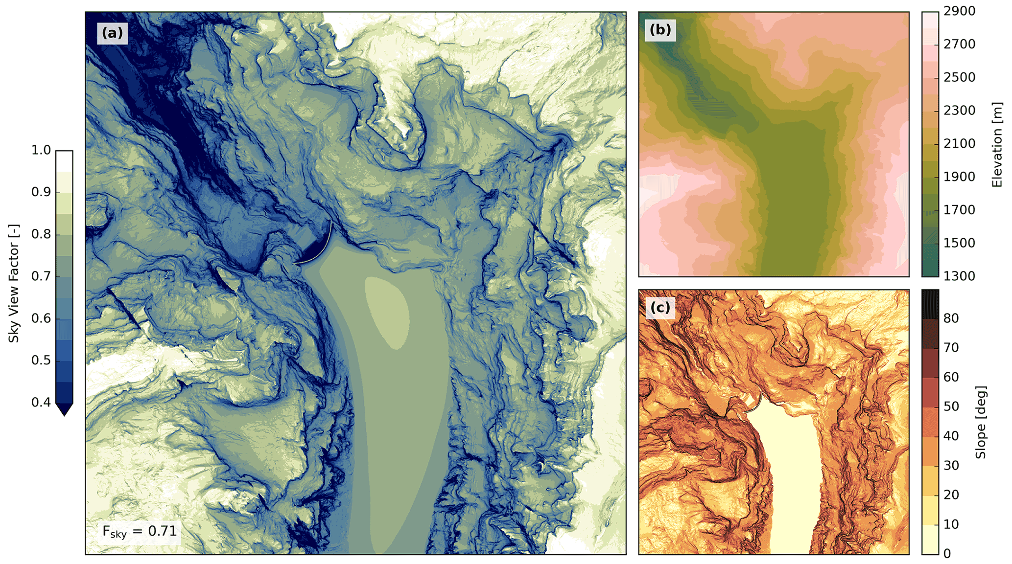
Figure 15Terrain parameters computed from the 2 m SwissALTI3D DEM for a 3 km wide domain centred at Limmerensee (Glarus Alps, Switzerland). Panel (a) illustrates the spatially gridded SVF, while the number in the lower left represents the domain-wide average. Panels (b) and (c) show the associated surface elevation and slope angles.
For the second considered domain (Fig. 15), the horizon search distance could be enhanced to 35 km. By considering the full DEM information, memory demands for the DEM data would have amounted to ∼16.0 GB – without considering memory needed to build the BVH. With terrain simplification, these demands dropped to ∼0.94 GB (∼867 MB for the inner domain and ∼73 MB for the outer TIN). In contrast to Fig. 14a, the spatially aggregated SVF is lower and averages to 0.71. This relatively low value is primarily caused by the deep gorge in the north-western part of the domain, which features a larger coherent area with SVF values below 0.5.
Horizon and derived SVF values are used in various fields and applications. Conventional horizon algorithms typically process the full elevation information along an azimuth sector's centreline, which makes them slow for (very) high-resolution DEMs. We propose a new and more efficient method, which is based on a high-performance ray-tracing library. In this approach, terrain information is stored in a tree structure (BVH) and only a fraction of elevation data have to be considered along a scanning line. A comparison of the ray-tracing-based horizon algorithm with a conventional method revealed its high computational performance, which amplifies for higher DEM resolutions and larger horizon search distances. The new algorithm exhibits only a minor performance dependency on horizon search distance, which allows computing more accurate horizon angles by considering larger search distances. Applying the horizon (and SVF) algorithm to larger domains can additionally be accelerated by masking water grid cells, whose minimal distance to the coastline is larger than the search distance for the horizon. In terms of accuracy, the ray-tracing-based algorithms agrees well with two existing methods in the case of larger distances (>1 km) between the sampling location and the horizon line. For smaller distances, deviations are larger. These discrepancies are caused by differences in internal terrain rendering. In the two reference algorithms, terrain is represented by quadrilaterals with a uniform elevation within individual cells, which results in a staircase-shaped surface. These structures translate to the computed horizon lines. In the new algorithm, terrain information is rendered by a triangle mesh, which represents a smooth continuous surface. Computed horizon lines subsequently have more natural gradients and do not suffer from staircase-shaped artefacts induced by terrain representation. A disadvantage of the new algorithm is its larger memory footprint, which is critical if very high-resolution DEM data are processed. However, these memory demands can be drastically lowered by simplifying terrain in the outer boundary zone of the DEM domain.
To infer SVF values from computed horizon angles, various methods are suggested in the literature (Dozier and Frew, 1990; Helbig et al., 2009; Manners et al., 2012), which are either applied in a horizontal or sloped coordinate system. We tested these methods for very steep and complex terrain and concluded that, in the case that horizon angles are available in a horizontal coordinate system, the method by Dozier and Frew (1990) is most convenient to apply. This SVF algorithm yields correct results for all terrains – even very steep and complex ones.
The terrain parameters horizon and/or sky view factor are applied in various numerical weather and climate models (Müller and Scherer, 2005; Chow et al., 2006; Senkova et al., 2007; Buzzi, 2008; Manners et al., 2012; Liou et al., 2013; Rontu et al., 2016; Arthur et al., 2018; Lee et al., 2019) to parameterise the effects of terrain geometry on surface radiation – either on the scale of the model grid or on a sub-grid scale. The relevance of the SVF for parameterising the effect of topography on surface radiation was confirmed in a recent study by Chu et al. (2021). They showed that, on domain-averaged scales, results from a three-dimensional ray-tracing simulation agree well with an SVF-based parameterisation. Even with our efficient horizon algorithm, the computation of sub-grid SVF is expensive for large weather and climate model domains. Fortunately, these sub-grid parameters have to be computed only once during the pre-processing stage of the model simulation. Nevertheless, it makes sense to compute them as efficiently as possible. We demonstrated that the computational time can be further reduced by considering less accurate horizon lines and by reducing the spatial sampling density. The loss in SVF accuracy is thereby only very minor. The speed-up factor grows with increasing resolution differences between the DEM and the target grid and exceeds 400 for the coarsest considered target resolution (25 km). The proposed method to efficiently computed sub-grid SVF provides a complement to the statistical method suggested by Helbig and Löwe (2014), which links SVF to local terrain parameters and is thus computationally very cheap. The choice of method depends on the available computational resources and the desired accuracy in SVF.
A run time analysis of our horizon algorithm revealed a considerable speed-up compared to conventional algorithms. However, performance could likely be further improved with the following suggestions, which concern the performance-critical ray-tracing part: we currently do not apply coherent rays in Embree, which allow for a more efficient utilisation of the BVH. Considering such ray streams might speed up horizon detection. To increase run times for workstations with performant graphic processing units (GPUs), ray casting could be performed with a GPU-based ray tracer, like NVIDIA OptiX (Parker et al., 2010).
Various Cartesian and elliptical (or spherical) coordinate systems are used in this work. In terms of Cartesian coordinates, we apply three different systems: ECEF , global ENU and local ENU coordinates. Equations to transform between the different reference systems are provided below.
A1 Transformation from geodetic to ECEF coordinates
Transformation from geodetic to ECEF coordinates is performed by
with and . ϕ represents the geodetic latitude, λ longitude, a the equatorial Earth radius (semi-major axis), b the polar Earth radius (semi-minor axis) and e the eccentricity.
A2 Transformation from ECEF to global ENU coordinates
Transformation from ECEF to global ENU coordinates is achieved by
with ϕr and λr representing the geodetic latitude and longitude. xr, yr and zr constitute the coordinates of the tangential point in ECEF coordinates. The transformation of a vector b from ECEF to global ENU coordinates is performed with
A3 Transformation between global and local ENU coordinates
We distinguish between two topocentric reference systems, the global and local ENU coordinates. The axes of the global ENU coordinate system do not coincide with local east, north and upward directions of all DEM grid cells. This is only true for local ENU coordinates. A vector b, expressed in global ENU coordinates (x′, y′ and z′), is converted to local ENU coordinates (x′′, y′′ and z′′) by
where R represents the rotation matrix. The inverse transformation requires the inverse of the rotation matrix R−1. Rotation matrices represent orthogonal matrices; thus, their inverse is identical to their transpose. The inverse transformation can subsequently be written as
The rotation matrix R is defined by
where ae, an and au represent the local ENU coordinate axes east, north and up in global ENU coordinates.
A4 Transformation between local ENU and spherical coordinates
In the local ENU coordinate system, we also apply spherical coordinates:
In this reference system, the azimuth angle φ is measured clockwise from north (y′′) and the elevation angle α is measured from the plane. In terms of the zenith angle ϑ, which is measured from up (z′′), the transformation can be expressed as
The elevation and zenith angles are linked via the relation .
A5 Conversion from orthometric to ellipsoidal height
Elevation data from DEMs often refer to orthometric heights. These elevations are measured relative to a geoid and must be converted to ellipsoidal heights if coordinates are subsequently transformed from a geodetic to a geocentric coordinate system. The relation between the ellipsoidal height he, the orthometric height ho and the geoid undulation N is specified by the following equation (Pillot et al., 2016; Grohmann, 2018):
For NASADEM data, we computed the undulation N based on EGM96 (Lemoine et al., 1998; NGA, 2021). For USGS arcsec elevation data, the GEOID12A geoid model (NGS, 2021) is applied. We bilinearly interpolate N from a 5 arcmin (EGM96) or 1 arcmin (GEOID12A) reference grid.
B1 Local east, north and upward unit vectors
Computing the horizon line for a certain location requires knowledge about the local direction vectors pointing towards east, north and up. We compute these unit vectors in ECEF coordinates according to the following equations. The upward vector is represented by the ellipsoid normal vector and can be computed as
This vector (au) is also called a geodetic normal or n vector. The vector an, pointing towards north and being perpendicular to vector au, can readily be derived in ECEF coordinates. First, the vector between the current location (vl) and the North Pole vp is computed as
The North Pole is given by . Vector vn is then projected on the location's normal plane to receive
Vector an is obtained by normalising vector vj:
The east unit vector (ae) is simply computed as
The direction vectors are subsequently transformed to global ENU coordinates with Eq. (A3).
B2 Slope aspect and angle of terrain
To compute the SVF, local terrain slope and aspect must be known, which can be represented by a local surface tilt vector. Various slope algorithms exist (Jones, 1998; Corripio, 2003) which typically consider the nearest four to eight DEM grid cells. We select an approach, in which a plane is fitted to the respective centre grid cell and its eight neighbours. The plane fitting is performed in the local ENU coordinate system by minimising the sum of squared z′′ differences between the plane and the nine cells. This approach requires solving a linear system of equations defined as
where n represents the surface normal of the sloped plane and x′′, y′′ and z′′ the DEM coordinates of the nine grid cells. The same method is used in the Geographic Information System software ArcGIS (ArcGIS, 2021).
HORAYZON is made available under the terms and conditions of the MIT license. The source code has been archived on Zenodo (https://doi.org/10.5281/zenodo.6965104, Steger, 2022) and is available on GitHub (https://github.com/ChristianSteger/HORAYZON, last access: 5 September 2022). HORAYZON's core dependencies are Intel Embree and Threading Building Blocks (TBB), as well as the NetCDF-4 C++ library and the Python packages Cython, NumPy, SciPy, GeographicLib, tqdm, requests and xarray. Dependencies can either be installed manually or conveniently via the package manager Conda. HORAYZON is a cross-platform application and supports both x86 and ARM architectures. On multi-core processor systems, HORAYZON can be run in parallel via TBB and OpenMP. All DEM data used in this study are freely available from the respective sources stated in the references.
CRS, BS and CS designed the research framework. Code implementation and data analysis were conducted by CRS. CRS, BS and CS were involved in writing and revising of the paper.
The contact author has declared that none of the authors has any competing interests.
Publisher's note: Copernicus Publications remains neutral with regard to jurisdictional claims in published maps and institutional affiliations.
Graphics were made using Python Matplotlib (version 3.4.3), PyVista (version 0.32.1), tikz (version 3.1.2) and Affinity Designer (version 1.10.4). Scientific colour maps of Crameri et al. (2020) are used.
This research has been supported by the Eidgenössische Technische Hochschule Zürich (grant no. ETH+03 19-2).
This paper was edited by Andrew Wickert and reviewed by Henning Löwe and Laura Rontu.
ArcGIS: Geodesic slope computation, https://pro.arcgis.com/en/pro-app/2.7/tool-reference/spatial-analyst/how-slope-works.htm, last access: 22 December 2021. a
Arnold, N. S., Rees, W. G., Hodson, A. J., and Kohler, J.: Topographic controls on the surface energy balance of a high Arctic valley glacier, J. Geophys. Res.-Earth, 111, F02011, https://doi.org/10.1029/2005JF000426, 2006. a
Arthur, R. S., Lundquist, K. A., Mirocha, J. D., and Chow, F. K.: Topographic Effects on Radiation in the WRF Model with the Immersed Boundary Method: Implementation, Validation, and Application to Complex Terrain, Mon. Weather Rev., 146, 3277–3292, https://doi.org/10.1175/MWR-D-18-0108.1, 2018. a, b
Ban, N., Caillaud, C., Coppola, E., Pichelli, E., Sobolowski, S., Adinolfi, M., Ahrens, B., Alias, A., Anders, I., Bastin, S., Belušić, D., Berthou, S., Brisson, E., Cardoso, R. M., Chan, S. C., Christensen, O. B., Fernández, J., Fita, L., Frisius, T., Gašparac, G., Giorgi, F., Goergen, K., Haugen, J. E., Hodnebrog, Ø., Kartsios, S., Katragkou, E., Kendon, E. J., Keuler, K., Lavin-Gullon, A., Lenderink, G., Leutwyler, D., Lorenz, T., Maraun, D., Mercogliano, P., Milovac, J., Panitz, H.-J., Raffa, M., Remedio, A. R., Schär, C., Soares, P. M. M., Srnec, L., Steensen, B. M., Stocchi, P., Tölle, M. H., Truhetz, H., Vergara-Temprado, J., de Vries, H., Warrach-Sagi, K., Wulfmeyer, V., and Zander, M. J.: The first multi-model ensemble of regional climate simulations at kilometer-scale resolution, part I: evaluation of precipitation, Clim. Dynam., 57, 275–302, https://doi.org/10.1007/s00382-021-05708-w, 2021. a
Behnel, S., Bradshaw, R., Citro, C., Dalcin, L., Seljebotn, D. S., and Smith, K.: Cython: The Best of Both Worlds, Comput. Sci. Eng., 13, 31–39, https://doi.org/10.1109/MCSE.2010.118, 2011. a
Bosch, J., Batlles, F., Zarzalejo, L., and López, G.: Solar resources estimation combining digital terrain models and satellite images techniques, Renew. Energ., 35, 2853 – 2861, https://doi.org/10.1016/j.renene.2010.05.011, 2010. a, b
Buzzi, M.: Challenges in operational numerical weather prediction at high resolution in complex terrain, PhD thesis, ETH Zurich, Switzerland, 2008. a, b, c, d, e, f, g, h, i
Calcabrini, A., Ziar, H., Isabella, O., and Zeman, M.: A simplified skyline-based method for estimating the annual solar energy potential in urban environments, Nature Energy, 4, 206–215, https://doi.org/10.1038/s41560-018-0318-6, 2019. a
Campos, R., Quintana, J., Garcia, R., Schmitt, T., Spoelstra, G., and M. A. Schaap, D.: 3D Simplification Methods and Large Scale Terrain Tiling, Remote Sensing, 12, 437, https://doi.org/10.3390/rs12030437, 2020. a
Chiodini, S., Pertile, M., Debei, S., Bramante, L., Ferrentino, E., Villa, A. G., Musso, I., and Barrera, M.: Mars rovers localization by matching local horizon to surface digital elevation models, in: 2017 IEEE International Workshop on Metrology for AeroSpace (MetroAeroSpace), 374–379, https://doi.org/10.1109/MetroAeroSpace.2017.7999600, 2017. a
Chow, F. K., Weigel, A. P., Street, R. L., Rotach, M. W., and Xue, M.: High-Resolution Large-Eddy Simulations of Flow in a Steep Alpine Valley. Part I: Methodology, Verification, and Sensitivity Experiments, J. Appl. Meteorol. Clim., 45, 63–86, https://doi.org/10.1175/JAM2322.1, 2006. a, b
Chu, Q., Yan, G., Qi, J., Mu, X., Li, L., Tong, Y., Zhou, Y., Liu, Y., Xie, D., and Wild, M.: Quantitative Analysis of Terrain Reflected Solar Radiation in Snow-Covered Mountains: A Case Study in Southeastern Tibetan Plateau, J. Geophys. Res.-Atmos., 126, e2020JD034294, https://doi.org/10.1029/2020JD034294, 2021. a
Codilean, A. T.: Calculation of the cosmogenic nuclide production topographic shielding scaling factor for large areas using DEMs, Earth Surf. Proc. Land., 31, 785–794, https://doi.org/10.1002/esp.1336, 2006. a
Codilean, A. T., Munack, H., Cohen, T. J., Saktura, W. M., Gray, A., and Mudd, S. M.: OCTOPUS: an open cosmogenic isotope and luminescence database, Earth Syst. Sci. Data, 10, 2123–2139, https://doi.org/10.5194/essd-10-2123-2018, 2018. a
Corripio, J. G.: Vectorial algebra algorithms for calculating terrain parameters from DEMs and solar radiation modelling in mountainous terrain, Int. J. Geogr. Inf. Sci., 17, 1–23, https://doi.org/10.1080/713811744, 2003. a
Crameri, F., Shephard, G. E., and Heron, P. J.: The misuse of colour in science communication, Nature Commun., 11, 5444, https://doi.org/10.1038/s41467-020-19160-7, 2020. a
Dirksen, M., Ronda, R., Theeuwes, N., and Pagani, G.: Sky view factor calculations and its application in urban heat island studies, Urban Climate, 30, 100498, https://doi.org/10.1016/j.uclim.2019.100498, 2019. a
Dozier, J. and Frew, J.: Rapid calculation of terrain parameters for radiation modeling from digital elevation data, IEEE T. Geosci. Remote, 28, 963–969, https://doi.org/10.1109/36.58986, 1990. a, b, c, d, e, f, g, h
Dozier, J., Bruno, J., and Downey, P.: A faster solution to the horizon problem, Comput. Geosci., 7, 145–151, https://doi.org/10.1016/0098-3004(81)90026-1, 1981. a, b, c, d
Dürr, B. and Zelenka, A.: Deriving surface global irradiance over the Alpine region from METEOSAT Second Generation data by supplementing the HELIOSAT method, Int. J. Remote Sens., 30, 5821–5841, https://doi.org/10.1080/01431160902744829, 2009. a, b
Embree: Intel Embree High Performance Ray Tracing, https://www.embree.org, last access: 22 December 2021. a, b
Fiddes, J., Aalstad, K., and Lehning, M.: TopoCLIM: rapid topography-based downscaling of regional climate model output in complex terrain v1.1, Geosci. Model Dev., 15, 1753–1768, https://doi.org/10.5194/gmd-15-1753-2022, 2022. a
Fogleman, M.: heightmap meshing utility (hmm), https://github.com/fogleman/hmm, last access: 22 December 2021. a
Garland, M. and Heckbert, P. S.: Fast Polygonal Approximation of Terrains and Height Fields, Tech. Rep. CMU-CS-95-181, Carnegie Mellon University, 1995. a
Grohmann, C. H.: Evaluation of TanDEM-X DEMs on selected Brazilian sites: Comparison with SRTM, ASTER GDEM and ALOS AW3D30, Remote Sens. Environ., 212, 121–133, https://doi.org/10.1016/j.rse.2018.04.043, 2018. a
Hao, D., Bisht, G., Gu, Y., Lee, W.-L., Liou, K.-N., and Leung, L. R.: A parameterization of sub-grid topographical effects on solar radiation in the E3SM Land Model (version 1.0): implementation and evaluation over the Tibetan Plateau, Geosci. Model Dev., 14, 6273–6289, https://doi.org/10.5194/gmd-14-6273-2021, 2021. a
Helbig, N. and Löwe, H.: Shortwave radiation parameterization scheme for subgrid topography, J. Geophys. Res.-Atmos., 117, D03112, https://doi.org/10.1029/2011JD016465, 2012. a
Helbig, N. and Löwe, H.: Parameterization of the spatially averaged sky view factor in complex topography, J. Geophys. Res.-Atmos., 119, 4616–4625, https://doi.org/10.1002/2013JD020892, 2014. a, b, c
Helbig, N., Löwe, H., and Lehning, M.: Radiosity Approach for the Shortwave Surface Radiation Balance in Complex Terrain, J. Atmos. Sci., 66, 2900–2912, https://doi.org/10.1175/2009JAS2940.1, 2009. a, b, c, d, e
Jacob, D., Petersen, J., Eggert, B., Alias, A., Christensen, O. B., Bouwer, L. M., Braun, A., Colette, A., Déqué, M., Georgievski, G., Georgopoulou, E., Gobiet, A., Menut, L., Nikulin, G., Haensler, A., Hempelmann, N., Jones, C., Keuler, K., Kovats, S., Kröner, N., Kotlarski, S., Kriegsmann, A., Martin, E., van Meijgaard, E., Moseley, C., Pfeifer, S., Preuschmann, S., Radermacher, C., Radtke, K., Rechid, D., Rounsevell, M., Samuelsson, P., Somot, S., Soussana, J.-F., Teichmann, C., Valentini, R., Vautard, R., Weber, B., and Yiou, P.: EURO-CORDEX: new high-resolution climate change projections for European impact research, Reg. Environ. Change, 14, 563–578, https://doi.org/10.1007/s10113-013-0499-2, 2014. a
Jones, K. H.: A comparison of algorithms used to compute hill slope as a property of the DEM, Comput. Geosci., 24, 315–323, https://doi.org/10.1016/S0098-3004(98)00032-6, 1998. a
Karney, C. F. F.: A python implementation of the geodesic routines in GeographicLib, https://geographiclib.sourceforge.io/html/python/, last access: 22 December 2021. a
Karney, C. F. F.: Algorithms for geodesics, J. Geodesy, 87, 43–55, https://doi.org/10.1007/s00190-012-0578-z, 2013. a, b
Karsisto, V., Nurmi, P., Kangas, M., Hippi, M., Fortelius, C., Niemelä, S., and Järvinen, H.: Improving road weather model forecasts by adjusting the radiation input, Meteorol. Appl., 23, 503–513, https://doi.org/10.1002/met.1574, 2016. a
Lee, W.-L., Liou, K.-N., Wang, C.-c., Gu, Y., Hsu, H.-H., and Li, J.-L. F.: Impact of 3-D Radiation-Topography Interactions on Surface Temperature and Energy Budget Over the Tibetan Plateau in Winter, J. Geophys. Res.-Atmos., 124, 1537–1549, https://doi.org/10.1029/2018JD029592, 2019. a, b
Lemoine, F., Kenyon, S., Factor, J., Trimmer, R., Pavlis, N., Chinn, D., Cox, C., Klosko, S., Luthcke, S., Torrence, M., Wang, Y., Williamson, R., Pavlis, E., Rapp, R., and Olson, T.: The development of the joint NASA GSFC and the National Imagery and Mapping Agency (NIMA) geopotential model EGM96, Tech. rep., National Aeronau- tics and Space Administration – Goddard Space Flight Center, Greenbelt, USA, 1998. a, b
Liou, K. N., Gu, Y., Leung, L. R., Lee, W. L., and Fovell, R. G.: A WRF simulation of the impact of 3-D radiative transfer on surface hydrology over the Rocky Mountains and Sierra Nevada, Atmos. Chem. Phys., 13, 11709–11721, https://doi.org/10.5194/acp-13-11709-2013, 2013. a, b
Manners, J., Vosper, S. B., and Roberts, N.: Radiative transfer over resolved topographic features for high-resolution weather prediction, Q. J. Roy. Meteor. Soc., 138, 720–733, https://doi.org/10.1002/qj.956, 2012. a, b, c, d, e, f, g, h, i, j
Marsh, C. B., Pomeroy, J. W., and Wheater, H. S.: The Canadian Hydrological Model (CHM) v1.0: a multi-scale, multi-extent, variable-complexity hydrological model – design and overview, Geosci. Model Dev., 13, 225–247, https://doi.org/10.5194/gmd-13-225-2020, 2020. a, b
Müller, M. D. and Scherer, D.: A Grid- and Subgrid-Scale Radiation Parameterization of Topographic Effects for Mesoscale Weather Forecast Models, Mon. Weather Rev., 133, 1431–1442, https://doi.org/10.1175/MWR2927.1, 2005. a, b
Nagy, B.: A New Method of Improving the Azimuth in Mountainous Terrain by Skyline Matching, J. Photogramm., 88, 121–131, https://doi.org/10.1007/s41064-020-00093-1, 2020. a
NASA JPL: NASADEM Merged DEM Global 1 arc second V001, NASA EOSDIS Land Processes DAAC [data set], https://doi.org/10.5067/MEaSUREs/NASADEM/NASADEM_HGT.001, 2020. a, b
NGA: Earth Gravitational Model 96, NGA [data set], https://earth-info.nga.mil, last access: 22 December 2021. a, b
NGS: GEOID12A, NGS [data set], https://geodesy.noaa.gov/GEOID/GEOID12A/, last access: 22 December 2021. a
Olson, M. and Rupper, S.: Impacts of topographic shading on direct solar radiation for valley glaciers in complex topography, The Cryosphere, 13, 29–40, https://doi.org/10.5194/tc-13-29-2019, 2019. a
Olson, M., Rupper, S., and Shean, D. E.: Terrain Induced Biases in Clear-Sky Shortwave Radiation Due to Digital Elevation Model Resolution for Glaciers in Complex Terrain, Front. Earth Sci., 7, 216, https://doi.org/10.3389/feart.2019.00216, 2019. a
Parker, S. G., Bigler, J., Dietrich, A., Friedrich, H., Hoberock, J., Luebke, D., McAllister, D., McGuire, M., Morley, K., Robison, A., and Stich, M.: OptiX: A General Purpose Ray Tracing Engine, ACM Trans. Graph., 29, https://doi.org/10.1145/1778765.1778803, 2010. a
Pillot, B.: DEM-based topography horizon model, https://www.mathworks.com/matlabcentral/fileexchange/59421-dem-based-topography-horizon-model (last access: 22 December 2021), 2016. a
Pillot, B., Muselli, M., Poggi, P., Haurant, P., and Dias, J. B.: Development and validation of a new efficient SRTM DEM-based horizon model combined with optimization and error prediction methods, Sol. Energy, 129, 101–115, https://doi.org/10.1016/j.solener.2016.01.058, 2016. a, b, c, d, e, f, g, h, i, j, k, l, m
Porter, C., Morin, P., Howat, I., Noh, M.-J., Bates, B., Peterman, K., Keesey, S., Schlenk, M., Gardiner, J., Tomko, K., Willis, M., Kelleher, C., Cloutier, M., Husby, E., Foga, S., Nakamura, H., Platson, M., Wethington, Michael, J., Williamson, C., Bauer, G., Enos, J., Arnold, G., Kramer, W., Becker, P., Doshi, A., D'Souza, C., Cummens, P., Laurier, F., and Bojesen, M.: ArcticDEM, Harvard Dataverse, V1 [data set], https://doi.org/10.7910/DVN/OHHUKH, 2018. a
Pritt, S. W.: Geolocation of photographs by means of horizon matching with digital elevation models, in: 2012 IEEE International Geoscience and Remote Sensing Symposium, 1749–1752, https://doi.org/10.1109/IGARSS.2012.6351180, 2012. a
Rontu, L., Wastl, C., and Niemelä, S.: Influence of the Details of Topography on Weather Forecast – Evaluation of HARMONIE Experiments in the Sochi Olympics Domain over the Caucasian Mountains, Front. Earth Sci., 4, 13, https://doi.org/10.3389/feart.2016.00013, 2016. a, b
Ruiz-Arias, J. A., Cebecauer, T., Tovar-Pescador, J., and Šúri, M.: Spatial disaggregation of satellite-derived irradiance using a high-resolution digital elevation model, Sol. Energy, 84, 1644–1657, https://doi.org/10.1016/j.solener.2010.06.002, 2010. a
Saurer, O., Baatz, G., Köser, K., Ladický, L., and Pollefeys, M.: Image Based Geo-localization in the Alps, Int. J. Comput. Vision, 116, 213–225, https://doi.org/10.1007/s11263-015-0830-0, 2016. a
Scarano, M. and Mancini, F.: Assessing the relationship between sky view factor and land surface temperature to the spatial resolution, Int. J. Remote Sens., 38, 6910–6929, https://doi.org/10.1080/01431161.2017.1368099, 2017. a
Senkova, A. V., Rontu, L., and Savijärvi, H.: Parametrization of orographic effects on surface radiation in HIRLAM, Tellus A, 59, 279–291, https://doi.org/10.1111/j.1600-0870.2007.00235.x, 2007. a, b, c
Sørland, S. L., Brogli, R., Pothapakula, P. K., Russo, E., Van de Walle, J., Ahrens, B., Anders, I., Bucchignani, E., Davin, E. L., Demory, M.-E., Dosio, A., Feldmann, H., Früh, B., Geyer, B., Keuler, K., Lee, D., Li, D., van Lipzig, N. P. M., Min, S.-K., Panitz, H.-J., Rockel, B., Schär, C., Steger, C., and Thiery, W.: COSMO-CLM regional climate simulations in the Coordinated Regional Climate Downscaling Experiment (CORDEX) framework: a review, Geosci. Model Dev., 14, 5125–5154, https://doi.org/10.5194/gmd-14-5125-2021, 2021. a
Steger, C: ChristianSteger/HORAYZON: HORAYZON v1.2 (v1.2), Zenodo [code], https://doi.org/10.5281/zenodo.6965104, 2022. a
Steppeler, J., Doms, G., Schättler, U., Bitzer, H. W., Gassmann, A., Damrath, U., and Gregoric, G.: Meso-gamma scale forecasts using the nonhydrostatic model LM, Meteorol. Atmos. Phys., 82, 75–96, https://doi.org/10.1007/s00703-001-0592-9, 2003. a
Swisstopo: Approximate formulas for the transformation between Swiss projection coordinates and- WGS84, https://www.swisstopo.admin.ch/content/swisstopo-internet/en/online/calculation-services/_jcr_content/contentPar/tabs/items/documents_publicatio/tabPar/downloadlist/downloadItems/19_1467104393233.download/ch1903wgs84_e.pdf (last access: 22 December 2021), 2016. a
Swisstopo: swissALTI3D, Federal Office of Topography swisstopo [data set], https://www.swisstopo.admin.ch/en/geodata/height/alti3d.html (last access: 5 September 2022), 2018. a, b
TBB: Intel Threading Building Blocks, https://github.com/oneapi-src/oneTBB, last access: 22 December 2021. a
USGS: 1/3rd arc-second Digital Elevation Models, USGS National Map 3DEP Downloadable Data Collection [data set], https://www.sciencebase.gov/catalog/item/4f70aa9fe4b058caae3f8de5 (last access: 5 September 2022), 2017a. a, b
USGS: 1 meter Digital Elevation Models, USGS National Map 3DEP Downloadable Data Collection [data set], https://www.sciencebase.gov/catalog/item/543e6b86e4b0fd76af69cf4c (last access: 5 September 2022), 2017b. a
Virtanen, P., Gommers, R., Oliphant, T. E., Haberland, M., Reddy, T., Cournapeau, D., Burovski, E., Peterson, P., Weckesser, W., Bright, J., van der Walt, S. J., Brett, M., Wilson, J., Millman, K. J., Mayorov, N., Nelson, A. R. J., Jones, E., Kern, R., Larson, E., Carey, C. J., Polat, İ., Feng, Y., Moore, E. W., VanderPlas, J., Laxalde, D., Perktold, J., Cimrman, R., Henriksen, I., Quintero, E. A., Harris, C. R., Archibald, A. M., Ribeiro, A. H., Pedregosa, F., van Mulbregt, P., and SciPy 1.0 Contributors: SciPy 1.0: Fundamental Algorithms for Scientific Computing in Python, Nature Methods, 17, 261–272, https://doi.org/10.1038/s41592-019-0686-2, 2020. a
Wald, I., Woop, S., Benthin, C., Johnson, G. S., and Ernst, M.: Embree: A Kernel Framework for Efficient CPU Ray Tracing, ACM Trans. Graph., 33, https://doi.org/10.1145/2601097.2601199, 2014. a, b
Wessel, P. and Smith, W. H. F.: A global, self-consistent, hierarchical, high-resolution shoreline database, J. Geophys. Res.-Sol. Ea., 101, 8741–8743, https://doi.org/10.1029/96JB00104, 1996. a
Zakšek, K., Oštir, K., and Kokalj, Ž.: Sky-View Factor as a Relief Visualization Technique, Remote Sensing, 3, 398, https://doi.org/10.3390/rs3020398, 2011. a
Zhang, Y. L., Li, X., Cheng, G. D., Jin, H. J., Yang, D. W., Flerchinger, G. N., Chang, X. L., Wang, X., and Liang, J.: Influences of Topographic Shadows on the Thermal and Hydrological Processes in a Cold Region Mountainous Watershed in Northwest China, J. Adv. Model. Earth Sy., 10, 1439–1457, https://doi.org/10.1029/2017MS001264, 2018. a, b
- Abstract
- Introduction
- Data
- Horizon and sky view factor algorithms
- Computational performance and accuracy of algorithms
- Application examples of the algorithms
- Conclusions
- Appendix A: Coordinate transformations
- Appendix B: Computation of auxiliary quantities
- Code and data availability
- Author contributions
- Competing interests
- Disclaimer
- Acknowledgements
- Financial support
- Review statement
- References