the Creative Commons Attribution 4.0 License.
the Creative Commons Attribution 4.0 License.
 | 28 Jul 2022
TransClim (v1.0): a chemistry–climate response model for assessing the effect of mitigation strategies for road traffic on ozone
Vanessa Simone Rieger
Volker Grewe
Road traffic emits not only carbon dioxide (CO2) and particulate matter, but also other pollutants such as nitrogen oxides (NOx), volatile organic compounds (VOCs) and carbon monoxide (CO). These chemical species influence the atmospheric chemistry and produce ozone (O3) in the troposphere. Ozone acts as a greenhouse gas and thus contributes to anthropogenic global warming. Technological trends and political decisions can help to reduce the O3 effect of road traffic emissions on climate. In order to assess the O3 response of such mitigation options on climate, we developed a chemistry–climate response model called TransClim (Modelling the effect of surface Transportation on Climate). The current version considers road traffic emissions of NOx, VOC and CO and determines the O3 change and its corresponding stratosphere-adjusted radiative forcing. Using a tagging method, TransClim is further able to quantify the contribution of road traffic emissions to the O3 concentration. Thus, TransClim determines the contribution to O3 as well as the change in total tropospheric O3 of a road traffic emission scenario. Both quantities are essential when assessing mitigation strategies. The response model is based on lookup tables which are generated by a set of emission variation simulations performed with the global chemistry–climate model EMAC (ECHAM5 v5.3.02, MESSy v2.53.0). Evaluating TransClim against independent EMAC simulations reveals low deviations of all considered species (0.01 %–10 %). Hence, TransClim is able to reproduce the results of an EMAC simulation very well. Moreover, TransClim is about 6000 times faster in computing the climate effect of an emission scenario than the complex chemistry–climate model. This makes TransClim a suitable tool to efficiently assess the climate effect of a broad range of mitigation options for road traffic or to analyse uncertainty ranges by employing Monte Carlo simulations.
- Article
(8454 KB) - Full-text XML
-
Supplement
(424 KB) - BibTeX
- EndNote


Mobility is getting more and more important in today's society. As residences, workplaces, schools and recreation areas are often spatially separated, there is an increasing demand on our transportation system. This leads to a steadily growing transportation volume and thus to steadily growing transportation emissions. Since 1970, emissions of greenhouse gases from transportation have more than doubled (Sims et al., 2014). In particular, emissions from road traffic play a significant role. Amongst all transportation sectors, the road traffic sector shows the largest growth rate. Emissions from this sector alone constitute more than 70 % of all greenhouse gas emissions originating from the transportation sector (Sims et al., 2014).
Road traffic emissions affect Earth's climate. Vehicles with combustion engines emit greenhouse gases such as carbon dioxide (CO2) and nitrous oxide (N2O). Greenhouse gases directly influence the radiation budget of the Earth and thus contribute to the anthropogenic global warming. In addition, road traffic emits also other pollutants, for example, nitrogen oxides (NOx), volatile organic compounds (VOCs), carbon monoxide (CO), sulfur dioxide (SO2) and particulate matter (PM) which also affect the atmospheric chemistry. For example, emissions of NOx, VOC and CO influence the ozone (O3) production and methane (CH4) destruction in the troposphere. These greenhouse gases in turn impact Earth's climate. The emissions of NOx, VOC and CO from road traffic increase the tropospheric O3 concentration and reduce the atmospheric lifetime of CH4 (Hoor et al., 2009). However, the process of forming and destroying O3 in the troposphere is non-linear. Whether O3 is produced or destroyed crucially depends on the background concentrations of NOx, VOC and CO. In rural areas, additional NOx emissions usually lead to an increase of the O3 concentration (so-called “NOx-limited” regime). But in regions with high NOx background concentrations, a further increase of NOx may even lead to a reduction of O3 (so-called “VOC-limited” regime, e.g. Dodge, 1977; Seinfeld and Pandis, 2006; Fowler et al., 2008).
Road traffic influences not only the climate, but it also contributes to air pollution. The compounds PM, O3, NO2 and SO2 penetrate deep into the lungs and thus can cause cardiovascular and respiratory diseases such as asthma and lung cancer. Consequently, emissions from road traffic increase the morbidity and mortality of the population (WHO, 2021). Besides the health impact of road traffic emissions, O3 harms sensitive plant species, which can cause a significant reduction of the quantity and quality of crop yields (Mills et al., 2007).
The impact of road traffic emissions on atmospheric chemistry and on climate has already been investigated by a number of studies (e.g. Reis et al., 2000; Niemeier et al., 2006; Matthes et al., 2007; Fuglestvedt et al., 2008; Hoor et al., 2009; Uherek et al., 2010; Righi et al., 2015; Mertens et al., 2018). Most studies show increasing ozone concentrations from road traffic emissions. For example at mid-latitudes, the surface concentration of O3 in the Northern Hemisphere increases by 5 %–15 % during summer but only up to 4 % during winter (Granier and Brasseur, 2003). However, road traffic emissions can also lead to a decrease of ozone. For example, during winter, Hoor et al. (2009) find an ozone decrease of 0.1 ppb in the lower troposphere over Europe. Moreover, Tagaris et al. (2015) focus on the influence of road traffic emissions on a regional scale, estimating an increase of maximum 8 h O3 mixing ratio by about 6.8 % over Europe. Hendricks et al. (2018) also investigate the climate effects of regional road traffic emissions. They reveal that German road traffic emissions contribute about 0.8 % to the total anthropogenic stratosphere-adjusted radiative forcing. They also derive a corresponding global mean surface temperature change of almost 0.005 K (for the year 2008).
To quantify the influence of road traffic emissions on O3, most model studies apply the perturbation method. This method compares the results of two model simulations: one simulation with all emissions (control simulation) and one simulation with perturbed emissions (experiment). Hence, it determines the change in total O3 concentration caused by perturbed emissions. In the following, this quantity is called impact. However for non-linear relationships such as the tropospheric O3 chemistry, the perturbation method is not suitable in determining the share of O3, which originates from emissions of a specific emission sector, for example, road traffic emissions (Grewe et al., 2010; Mertens et al., 2020). Changes in one emission sector also affect the O3 production from other emission sectors as O3 precursors from different emission sectors are competing with each other in producing O3. For example, when reducing NOx from road traffic emissions, NOx from other sectors can produce O3 more efficiently. Thus, it is important to determine the contribution of the emission sectors to O3. Grewe et al. (2010) propose the application of the so-called tagging method. It follows the most important reaction pathways for the formation and destruction of O3 and thus determines the contribution of road traffic emissions to the O3 concentration. Accordingly, the perturbation method determines the impact and the tagging method determines the contribution of road traffic emissions to O3. Both methods are essential to assess the total effect of road traffic emissions on climate. (In the following, we use the term “effect” when referring to the impact and contribution together.) A detailed overview on the characterization and applicability of the two methods is given in Table 1 of Mertens et al. (2020).
Ozone is not only harmful for the health of humans, animals and plants, it also acts as a greenhouse gas contributing to global warming. Consequently, it is crucial to reduce road traffic emissions to minimize the effect on climate. For this purpose, different mitigation options are available, ranging from technical innovations to driving bans (e.g. Sims et al., 2014). On the one hand, new technological trends such as new fuels for passenger cars, heavy goods vehicles and buses (e.g. Karavalakis et al., 2012; Suarez-Bertoa et al., 2015; Jedynska et al., 2015) change the vehicles' emissions of NOx, VOC and CO and thus impact Earth's climate. On the other hand, political decisions such as financial support for electrical cars and car pooling also influence climate. Each mitigation option acts differently on O3 and thus on climate. Hence, the quantification of the climate response is essential to fully assess a mitigation option.
Typically, complex chemistry–climate models are applied to assess the climate effect of traffic emissions. But these simulations are computationally expensive and require a substantial amount of time. This impedes the assessment of many mitigation scenarios. Hence, we developed a new tool called TransClim (Modelling the effect of surface Transportation on Climate). It is a chemistry–climate response model which efficiently determines the O3 effect on climate for road traffic emission scenarios. TransClim is able to consider a broad range of road traffic emission scenarios such as the introduction of biofuels in North America or driving bans of road traffic over Europe or Asia. The current version of TransClim determines the impact and contribution of road traffic emission scenarios on O3. Moreover, it quantifies the contribution of emissions to the destruction of methane, as well as the variation in CH4 lifetime caused by changes of the hydroxyl radical (OH). Methane as a precursor of ozone is not regarded.
Here, we present the response model TransClim and provide an assessment of the model's skills. The paper is structured as follows: in Sect. 2, the response model TransClim is described. Then, TransClim is evaluated against simulations with the global chemistry–climate model EMAC in Sect. 3. Section 4 gives an overall assessment of the response model.
The work presented in this paper is based on the PhD thesis by V. S. Rieger. Hence, significant parts of the text have already appeared in Rieger (2018).
2.1 Overview
The new tool TransClim is a chemistry–climate response model which efficiently assesses the climate effect of changes in road traffic emissions. To quickly determine the climate effect of a given emission scenario, TransClim does not explicitly calculate the chemical and physical processes. Instead, it uses lookup tables (LUTs) which contain precalculated relationships between emissions and their climate effects. Road traffic emissions of NOx, VOC and CO are varied, and the corresponding climate effect is simulated with the global chemistry–climate model EMAC (see details in Sect. 2.4.1). These relationships between emission variation and climate effect are used to create lookup tables (LUTs) for TransClim. TransClim interpolates within these LUTs and determines the climate effect of a specific road traffic emission scenario.
TransClim focuses on the O3 effect of road traffic emissions on climate. Using the precalculated relationships, it can also determine the effect of road traffic emission changes on other variables such as OH or NOx. It is further able to calculate the resulting radiative forcings by determining the stratosphere-adjusted radiative flux changes at the top of the atmosphere. Moreover, TransClim is able to quantify the contribution of road traffic emissions to O3, OH and the radiative flux by using a tagging method which is implemented in EMAC (Grewe et al., 2010, 2017). This tagging method is described in Sect. 2.2.
2.2 Tagging method
To attribute the effect of road traffic emissions on tropospheric ozone, we use a tagging method (Grewe et al., 2010; Grewe, 2013; Grewe et al., 2017; Rieger et al., 2018). It considers 10 source categories: emissions from the sectors anthropogenic non-traffic (e.g. industry and households), road traffic, ship traffic, air traffic, biogenic sources, biomass burning, lightning, methane (CH4) and nitrous oxide (N2O) decompositions and stratospheric ozone production. The tagging method computes the contributions of these 10 source categories to seven chemical species or chemical families: O3, hydroxyl radical (OH), hydroperoxyl radical (HO2), CO, peroxyacyl nitrates (PAN), reactive nitrogen compounds (NOy; e.g. NO, NO2, HNO4, ...) and non-methane hydrocarbons (NMHCs). Like an accounting system, this method follows all important reaction pathways for the production and destruction of the regarded species.
As an example, a bimolecular reaction of the chemical species A and B forming the species C is considered (see also Grewe et al., 2010):
Each species A,B and C is split up into the 10 subspecies Ai,Bi and Ci. Thus, Ai describes the contribution of the source category i to the concentration of A (the same holds for Bi and Ci). These tagged species () go through the same reactions as their main species (). In general, if A from the category i reacts with B from category j, half of the formed C is attributed to category i and half to the category j:
Regarding all possible combinations of the reaction of Ai with Bj, the production of Ci is deduced mathematically by a combinatorial approach and eventually leads to (see Grewe et al., 2010, for more details)
with k being the reaction rate coefficient of Reaction (R1). Consequently, this combinatorial approach enables a full partitioning of the reaction rate.
In this manner, the tagging method used in this study determines the contribution of road traffic emissions to ozone. In the following, this variable is denoted by O. Thus, a change in road traffic emissions varies not only the total ozone concentration (impact), but also the contribution of road traffic emissions. Both quantities together, the impact and the contribution, give a complete understanding of how road traffic emissions influence ozone.
2.3 Objectives
The aim of TransClim is to assess the effect of road traffic emissions of NOx, VOC and CO on tropospheric O3 and its respective effect on climate (e.g. radiative forcing). Thus, the algorithm of TransClim, which combines precalculated relationships between emissions and climate effect, needs to meet the following objectives:
-
Based on road traffic emissions of NOx, VOC and CO, the algorithm determines the total change in O3 concentration as well as the contribution of road traffic emissions to the O3 concentration (O, derived by the tagging method; see Sect. 2.2).
-
As the O3 chemistry in the troposphere is non-linear, it is important that the algorithm includes these non-linearities.
-
Road traffic emissions originating from different emission regions (e.g. Europe, North America, ...) are accounted for.
-
The algorithm determines the geographical pattern of the O3 and O change resulting from a given road traffic emission scenario. This allows for assessing not only the global, but also the regional effects as the remote effect can differ from the local source region effect.
-
The stratosphere-adjusted radiative forcings of O3 and O are calculated.
-
The algorithm is computational very efficient. This means that the climate effect (e.g. radiative forcing) of a given emission scenario is calculated within minutes or hours. Differences in the results compared with complex chemistry–climate model simulations generally remain below 10 %.
2.4 Calculation of lookup tables
2.4.1 Model description of global chemistry–climate model EMAC
We use the global chemistry–climate model ECHAM/MESSy Atmospheric Chemistry (EMAC) to generate the LUTs for TransClim. EMAC is a numerical chemistry and climate simulation system that includes sub-models describing tropospheric and middle atmosphere processes and their interaction with oceans, land and human influences (Jöckel et al., 2010). It uses the second version of the Modular Earth Submodel System (MESSy2) to link multi-institutional computer codes. The core atmospheric model is the fifth-generation European Centre Hamburg general circulation model (ECHAM5; Roeckner et al., 2006). For the present study, we applied EMAC (ECHAM5 version 5.3.02, MESSy version 2.53.0) in the T42L90MA resolution, i.e. with a spherical truncation of T42 (corresponding to a quadratic Gaussian grid of approx. 2.8 by 2.8∘ in latitude and longitude) with 90 vertical hybrid pressure levels up to 0.01 hPa. The applied model setup is similar to the model setup of the EMAC simulation RC1SD-base-10a described in detail in Jöckel et al. (2016). In the following, the most important configuration features of the simulation are summarized. The simulation is free-running, i.e. it is not constrained by observational atmospheric data, but the prognostic variables such as vorticity and divergence are calculated from the primitive equations. The time step length is 12 min.
The chemical mechanism is solved by the submodel MECCA (Module Efficiently Calculating the Chemistry of the Atmosphere; Jöckel et al., 2010; Sander et al., 2011) which regards the basic chemistry of the troposphere and stratosphere. It considers 188 chemical species interacting in 218 gas-phase, 12 heterogeneous and 68 photolysis reactions.
To detect small perturbations (such as variations in emissions of road traffic), we apply the Quasi Chemistry Transport Model (QCTM) mode for EMAC (Deckert et al., 2011). It decouples the chemistry from the dynamics by prescribing climatologies for the radiation calculation and the hydrological cycle. As a result, a chemical perturbation can not modify the atmospheric dynamics. This method reduces the “noise” in the model simulation and hence enables the quantification of the climate response to a small perturbation.
To specify the contribution of road traffic emissions to the O3 concentration (), the submodel TAGGING is used. Without affecting the chemistry, the method enables the quantification of the contribution of 10 source categories to the chemical species (see Sect. 2.2).
The radiative fluxes are computed by the submodel RAD (Dietmüller et al., 2016). The longwave radiative spectrum is divided into 16 spectral bands (Mlawer et al., 1997). The shortwave radiative spectrum consists of 4 spectral bands in the troposphere and up to 55 bands in the stratosphere and mesosphere (Fouquart and Bonnel, 1980; Nissen et al., 2007). EMAC offers the possibility to calculate radiative fluxes multiple times:
-
The radiative fluxes calculated by the first call of the radiation module are used to feed back to the model simulation. As EMAC is run in the QCTM mode (Quasi Chemistry Transport Model mode; see above), these instantaneous radiative fluxes are based on climatologies of CO2, CH4, O3, N2O, CF2Cl2 and CFCl3.
-
In contrast to the first call which uses climatologies for O3, the second call of the radiation module computes the stratosphere-adjusted radiative fluxes of the perturbed O3 field. The perturbed O3 field is calculated by the model chemistry (provided by the submodel MECCA). It refers to the MECCA ozone field and the road traffic tagged ozone and by that includes changes in road traffic emissions. Here, we call the resulting net radiative flux flxn(O3).
-
The third call of the radiation module determines the stratosphere-adjusted radiative fluxes of the difference field (O3–) which corresponds to the share of O3, excluding O3 from road traffic. In this case, O3 and are also computed by the model chemistry and regard emission changes of road traffic. The resulting net radiative flux is labelled flxn(O3–).
In a post-processing step, the radiation fluxes calculated by the second and third call of the radiation module are subtracted from each other to obtain the net radiative flux caused by the contribution of road traffic emissions to ozone (Mertens et al., 2018):
Anthropogenic emissions such as emissions from road traffic, ships, aviation, industry, agricultural waste burning and biomass burning are provided by the MACCity emission inventory (Granier et al., 2011). The submodel ONEMIS (Kerkweg et al., 2006) computes emissions during the simulation (i.e. online) such as emissions of soil NOx (following Yienger and Levy, 1995) and biogenic isoprene (C5H8) emissions (following Guenther et al., 1995).
For NOx from lightning, the parameterization of Grewe et al. (2001) is applied with lightning NOx emissions scaled to approx. 5 Tg(N) yr−1.
The time period of July 2009 to December 2010 is simulated. The first half-year is taken as a spin-up period; the year 2010 is used for the analysis. Due to limited computational resources, it is only possible to use 1 year for the analysis. An EMAC simulation performed for a time period of 3 years shows that the year-to-year variability of tropospheric O3 and O is quite low, which allows for using only 1 year for the analysis (see also Hoor et al., 2009; Van Dingenen et al., 2018).
2.4.2 Emission regions
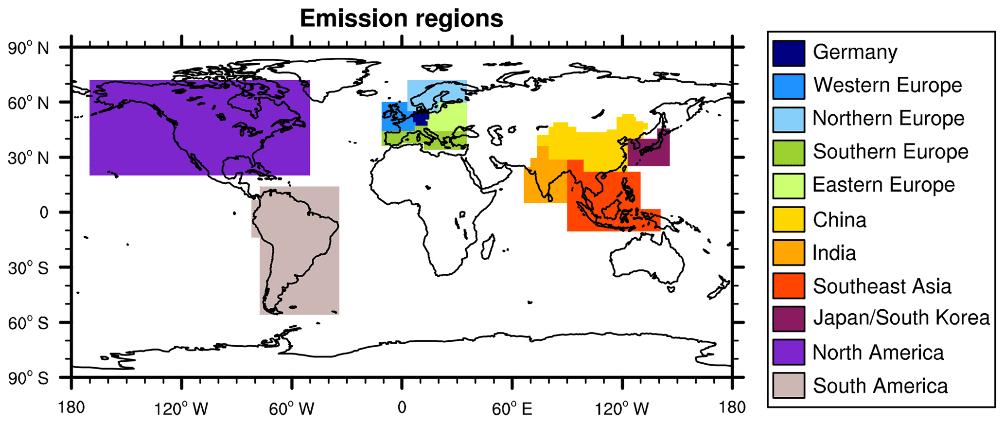
Figure 1Emission regions which are defined for the LUTs of TransClim.
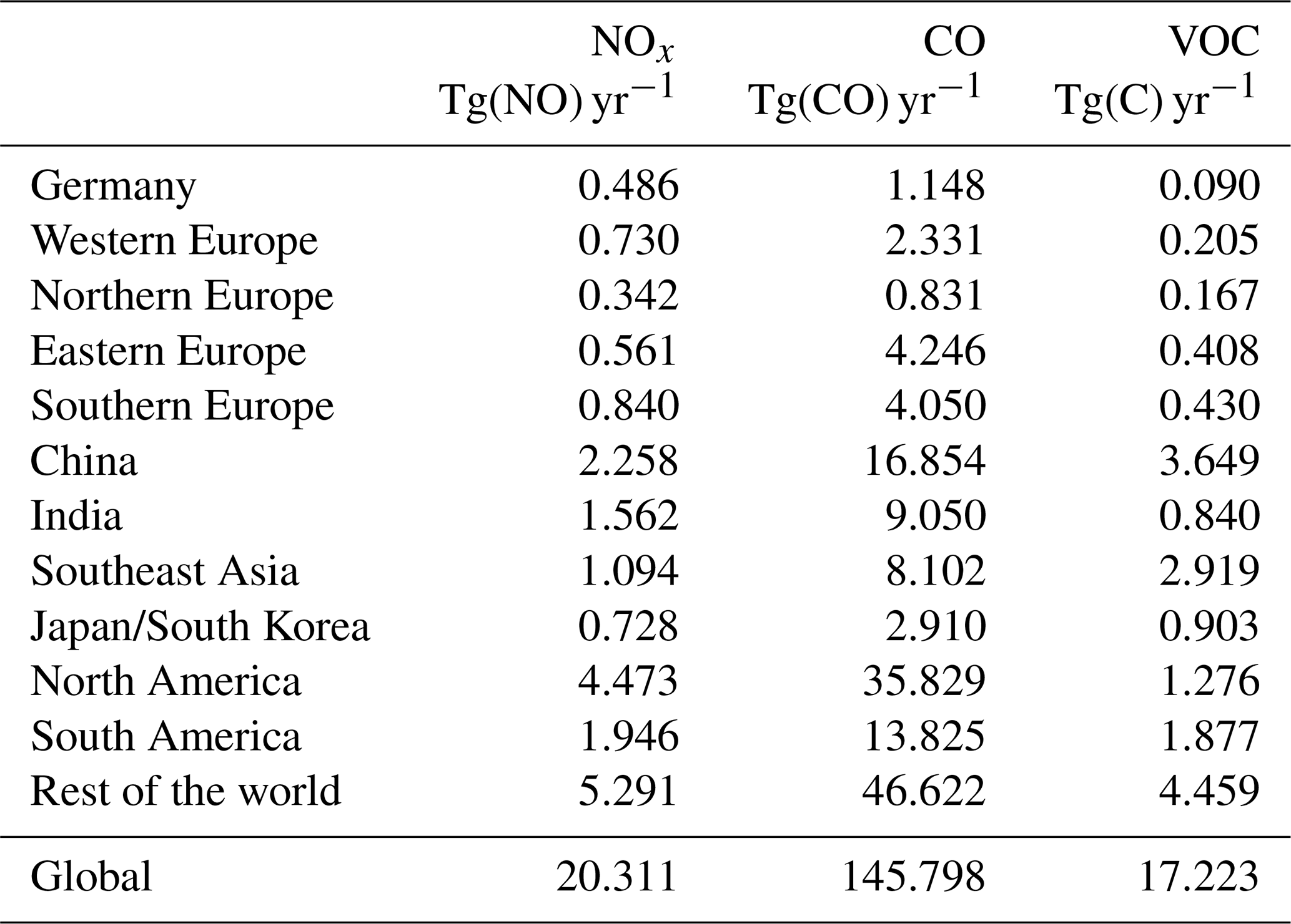
To determine the effect of road traffic emissions from different parts of the world, 11 emission regions are defined (Fig. 1): Germany, Western Europe, Northern Europe, Eastern Europe, Southern Europe, North America, South America, China, India, Southeast Asia and Japan/South Korea. Table 1 gives the total amounts of road traffic emissions for NOx, CO and VOC in the 11 emission regions, the remaining part of the world and the global values as derived from the emission inventory MACCity (Granier et al., 2011). The emission region Germany has low VOC road traffic emissions of only 0.09 Tg(C) yr−1 compared to the other European emission regions. Eastern and Southern Europe show high CO road traffic emissions of about 4 Tg(CO) yr−1. The emission regions China, India and Southeast Asia as well as North and South America have high road traffic emissions in 2010. The global road traffic emissions for NOx are 20.31 Tg(NO) yr−1, for CO 145.80 Tg(CO) yr−1 and for VOC 17.22 Tg(C) yr−1 in 2010.
Russia, Africa, Arabian Peninsula and Australia are not regarded as a separate emission region yet. However, this set of emission regions is not fixed. The LUTs can be easily expanded by performing additional emission variation simulations with EMAC. In this manner, further emission regions can be considered, or one emission region can be split up into smaller emission regions if needed.
Table 1Road traffic emissions per emission region for the year 2010 derived from the emission inventory MACCity (Granier et al., 2011). Global emissions are given in the last row.
2.4.3 Setup of emission variation simulations
To generate the LUTs, emission variation simulations are performed with EMAC. Emission scaling factors for NOx, VOC and CO road traffic emissions (sNOx, sVOC, sCO) are defined which describe the factors by which the emissions of the EMAC reference simulation are scaled. In each of the 11 emission regions (see Sect. 2.4.2), these emission scaling factors are varied, and a simulation is performed with EMAC. The respective EMAC output for the year 2010 is used as input for the LUTs.
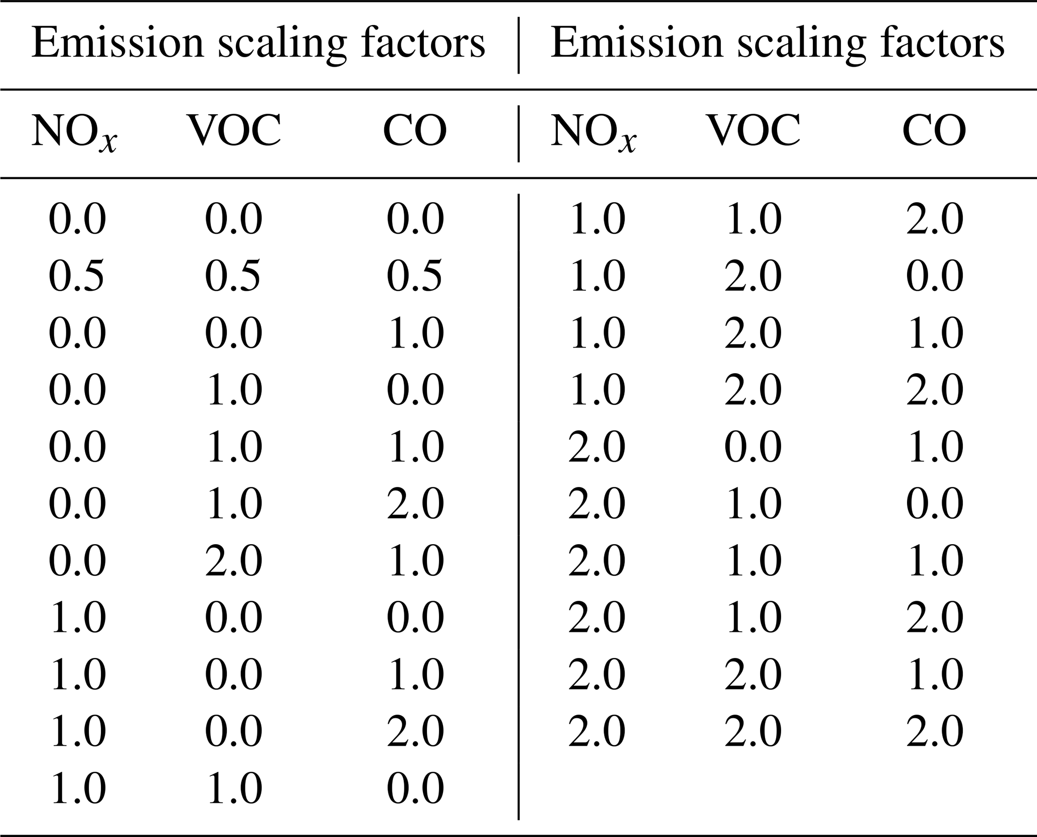
First of all, an EMAC reference simulation is performed with all emission scaling factors (sNOx, sVOC, sCO) in all emission regions set to 1. Then, sNOx, sVOC and sCO are changed in one of the 11 emission regions, while the factors of the remaining emission regions are kept constant at 1. As it is computationally too expensive to cover the whole domain of possible emission variations of NOx, VOC and CO, one of the emission scaling factors is always kept fixed at 1. This means either two emission scaling factors are varied at the same time while the third factor is left at 1, or one emission scaling factor is varied while the other two factors are kept at 1. For the current set of LUTs, emission variation simulations with EMAC are performed using emission scaling factors varied between 0 (corresponding to no emissions) and 2 (corresponding to a duplication of emissions) in each emission region. Additionally, three emission variation simulations with sNOx, sVOC and sCO set all to 0, 0.5 and 2 in each emission region are conducted. Table 2 shows a list of all emission variation simulations performed with EMAC: in total 21 emission variation simulations per emission region are currently available.
Table 2List of emission variation simulations performed with EMAC for each emission region. This set is used as input for the LUTs for TransClim.
2.5 Algorithm
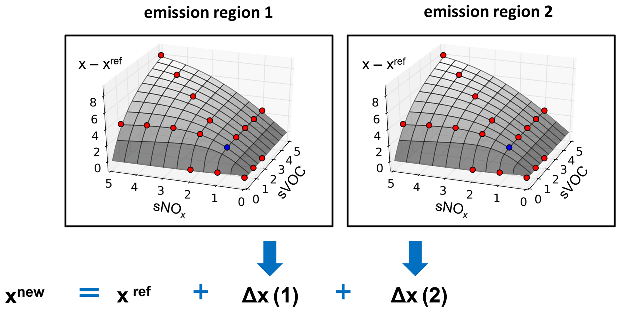
Figure 2Schematic of interpolation algorithm used by TransClim. For each emission region, a LUT contains the change in variable x (x−xref) and the emission scaling factors for NOx, VOC and CO emissions (sNOx, sVOC, sCO). In the figure, only sNOx and sVOC are displayed. The blue dot indicates the reference simulation (). The red dots indicate the emission variation simulations (note that the red dots are just a schematic and do not represent the actual emission scaling; see Table 2). After linearly interpolating within the LUT for each emission region i, the resulting changes Δx(i) are added to reference xref. This procedure is performed for every grid box or for tropospheric or global means.
This section describes how the emission variation simulations performed with EMAC (see Sect. 2.4.3) are combined to generate an efficient algorithm for TransClim. Rieger (2018) tested several algorithms, and the algorithm which produced the best results is used in TransClim and described here. For the sake of clarity, Fig. 2 shows a schematic of the algorithm for only two emission regions (e.g. Western and Eastern Europe) and for only two road traffic emission species NOx and VOC. For each emission region, the emission variation simulations performed with EMAC are used to create a LUT. The emission scaling factors for NOx, VOC and CO road traffic emissions (sNOx, sVOC, sCO), which describe the factors by which the emissions of the EMAC reference simulation are scaled, are used as input variables. Thus, each LUT has three dimensions: sNOx, sVOC and sCO (in Fig. 2, two dimensions). The LUT then provides the change (Δx) of a variable x with respect to the EMAC reference simulation (xref). Recall that, for the EMAC reference simulation, all emission scaling factors of all emission regions are set to 1. Consequently, each variable x (e.g. O3, , OH, OHtra, flxn(O3), flxn()) has its own LUT.
To obtain the desired variable xnew for a given road traffic emission scenario, the corresponding emission scaling factors (sNOx, sVOC, sCO) for each emission region i are used as input, and the change Δx(i) for each emission region is calculated by linearly interpolating within the respective LUT. Since for example an emission change of NOx in one emission region affects also the O3 concentration in an emission region which is far away from the source region, it is important to consider the effect of all emission regions together. Thus for each grid box b, the computed Δx(i) of each emission region i is added to xref from the EMAC reference simulation (see Fig. 2):
This method can be applied either for each grid box of the three-dimensional emission variation simulations or for the tropospheric or global mean of a variable x. (The tropospheric or global mean of the respective variable was computed in advance during the post-processing of the emission variation simulations.) Hence, the red dots in Fig. 2 can show the data of a one-dimensional variable (e.g. global radiative forcing) or the data of a three-dimensional variable for one grid box (e.g. O3 concentration). For a three-dimensional field, the emission scaling factors are applied to all grid boxes of the three-dimensional responses and added to the EMAC reference simulation to obtain the three-dimensional response xnew.
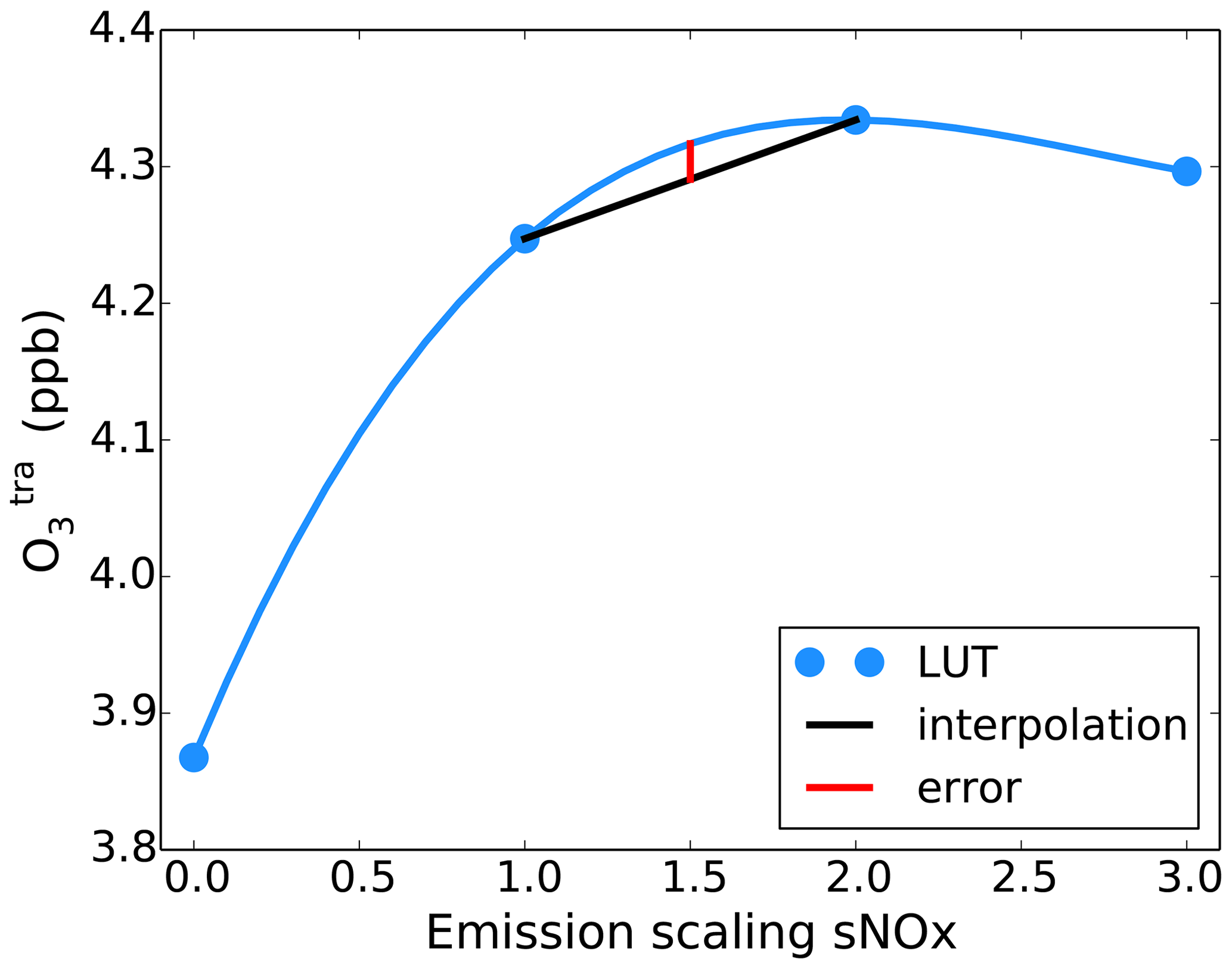
In general, this algorithm leads to an underestimation of the computed variables in comparison to the EMAC results. Figure 3 shows a schematic of the interpolation error of the variable calculated by TransClim. Blue dots indicate the LUT values for depending on the NOx emission scaling factors in Germany. The blue line presents the non-linear relationship between the NOx emissions and . The interpolation algorithm of TransClim is implemented in Python. The LUTs of TransClim are three-dimensional, and the data are arranged on an irregular grid. For an interpolation in a multi-dimensional irregular data structure, the library SciPy in Python only offers the option to interpolate linearly within this grid. The curvature of the non-linear relationship between NOx emissions and is negative. Thus, a linear interpolation within the LUT (indicated by the black line) causes an underestimation of the interpolated value. The error which is caused by the linear interpolation is indicated with the red line. However, the resulting errors are so small (see Sect. 3) that the application of a linear interpolation is justified.
The approach, presented in this section, offers a fast method to estimate the effect of road traffic emissions on, for example, tropospheric O3. Using a standard computer1, it takes 0.2 s to compute the global mean climate effect of an emission scenario in one emission region. To calculate a three-dimensional variable, for example, the new O3 concentration in the whole atmosphere, for an emission scenario, it takes about 15 min. In this case, the algorithm is applied to each grid box of a global climate simulation: to 64 latitudes, 128 longitudes and 90 vertical pressure levels (this is the resolution of the global chemistry–climate model EMAC used to generate the LUTs; see Sect. 2.4).
2.6 Workflow of TransClim

Figure 4Workflow of TransClim showing the main calculation steps. For a defined emission and control scenario, TransClim computes the resulting climate effect such as the stratosphere-adjusted radiative forcing at the top of the atmosphere.
Figure 4 shows the workflow of the main calculation steps performed by TransClim. To quantify the climate effect of an emission scenario with TransClim, a suitable control scenario (e.g. no road traffic emissions in Europe) has to be defined as well. This is important for determining a radiative forcing.
First of all, all required input data from the emission variation simulations performed with EMAC (see Sect. 2.4.3) are read (the input variables are listed in Table S4 in the Supplement). Based on this input data from the emission variation simulations, TransClim creates LUTs with the dimensions sNOx, sVOC and sCO representing the variable change x−xref for each emission region and each grid box. For example, for the tropospheric mean of O3, 11 LUTs for the 11 emission regions are produced. For the three-dimensional variable O3, TransClim generates in total 8 110 080 LUTs (11 emission regions × 90 levels × 64 latitudes × 128 longitudes).
Afterwards, TransClim computes the variables for a given emission and control scenario applying the algorithm described in Sect. 2.5. As a first step, the algorithm considers the set of emission scaling factors which have been defined for the emission and control scenario and then linearly interpolates within the LUTs to obtain the change of the variable x with respect to the EMAC reference simulation Δxb(i). This procedure is repeated for each emission region i and each grid box b. In a second step, the interpolated results of each emission region are added to the value of the reference EMAC simulation: , with n being the number of emission regions (here n=11).
Subsequently, the stratosphere-adjusted radiative forcings for O3 and O at the top of the atmosphere of the emission scenario with respect to the control scenario are calculated by subtracting the radiative fluxes which have been determined in the previous steps by TransClim. In a final step, the interpolated values for the emission and control scenario are written to netCDF files.
In the following section, the model TransClim is evaluated against the global model EMAC. Firstly, TransClim is compared with equivalent EMAC simulations for road traffic emission changes over various emission regions and for different strengths of emission scaling in one emission region. Secondly, TransClim is evaluated against other EMAC simulations performed within the DLR project VEU1 (Verkehrsentwicklung und Umwelt 1, i.e. Transport and the Environment 1, https://verkehrsforschung.dlr.de/projekte/veu, last access: 20 July 2022; Hendricks et al., 2018).
3.1 Comparison with equivalent EMAC simulations
3.1.1 Road traffic emission changes over Europe
In this section, the road traffic emissions in Europe are varied, and the corresponding TransClim simulation is compared with an equivalent EMAC simulation. Based on the emission variation simulations which are currently available for the LUTs of TransClim (see Sect. 2.4.3), a set of emission scaling factors for each emission region in Europe is chosen in such a way that a broad range of emission variation is given. The values for the emission scaling factors in Europe are summarized in Table 3. The road traffic emissions of NOx, VOC and CO are only changed in Europe to test if the algorithm of TransClim also works on a regional scale. Here, the non-linearities of the O3 chemistry are expected to be larger than on a global scale. Hence, this scenario with a large variation of emissions in Europe is expected to be a difficult test case for TransClim.
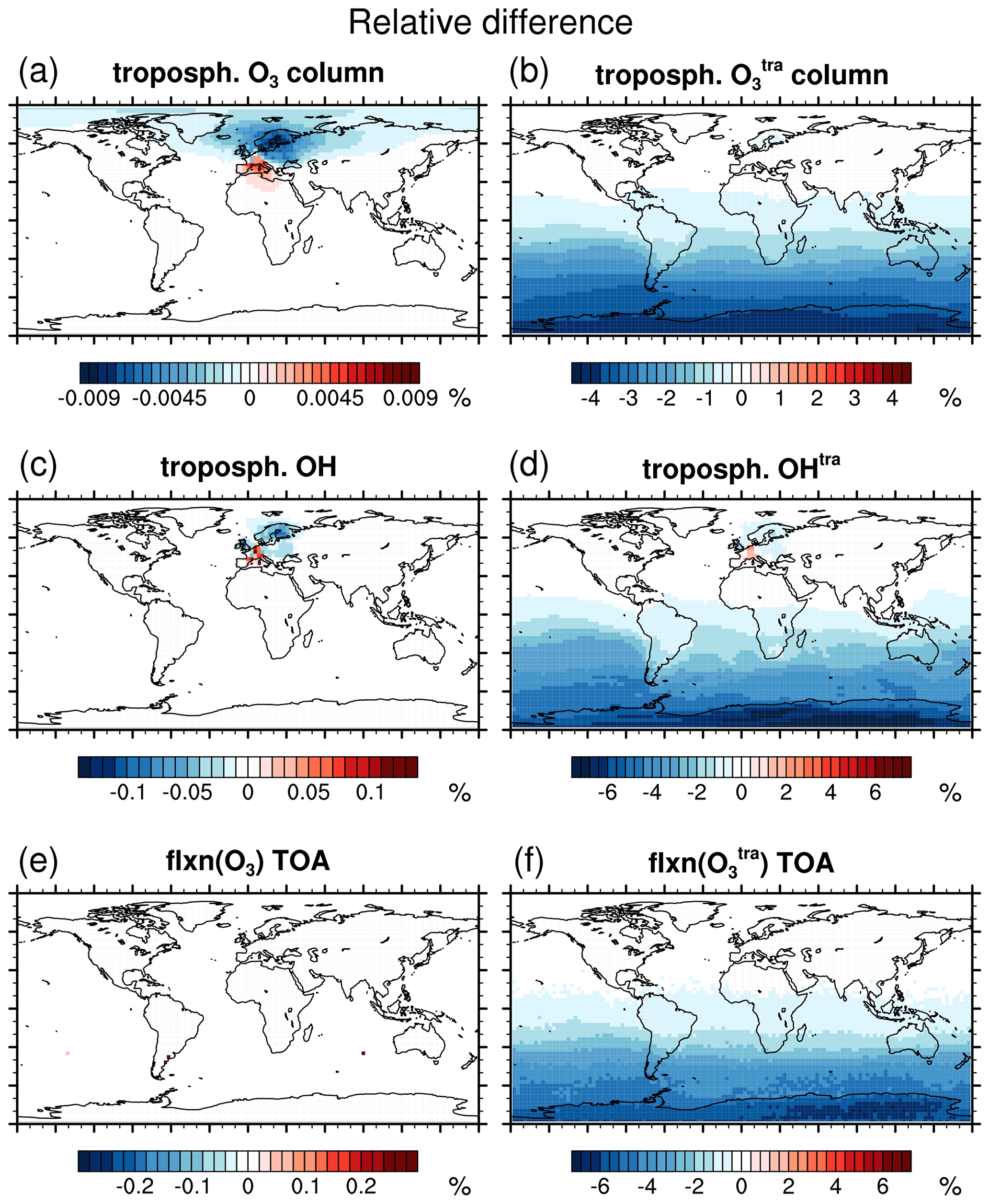
Figure 5Relative difference between TransClim and EMAC simulation. Ozone (O3), hydroxyl radical (OH) and ozone net radiative fluxes (flxn(O3)) as well as the contributions to ozone (), to hydroxyl radical (OHtra) and to ozone net radiative fluxes (flxn(O)) are shown. For O3 and , the relative difference of the tropospheric columns is shown (a, b). For OH and OHtra, the deviations of the tropospheric means are displayed (c, d). The values at the top of the atmosphere (TOA) are shown for flxn(O3) and flxn(O) (e, f).
For the comparison, the emission scaling factors listed in Table 3 are used for a simulation with EMAC (see Sect. 2.4.1) and for a simulation with TransClim (based on the LUTs as described in Sect. 2.4.3). The relative differences between the TransClim and the EMAC simulation for the variables tropospheric ozone column (O3), tropospheric mean of hydroxyl radical (OH) and net radiative flux caused by O3 at the top of the atmosphere (flxn(O3)) as well as the corresponding contributions of road traffic emissions (, OHtra, flxn(O)) are shown in Fig. 5. (The absolute values are shown in the Appendix, Fig. A1.) For the tropospheric O3 column, the largest deviations of −0.009 % are found in Northern Europe and span over the Northern Hemisphere. Deviations of up to 0.1 % in the tropospheric mean of OH are only found over Europe. For the net radiative flux flxn(O3), the relative differences between EMAC and TransClim are very small (in average <0.001 %).
The contributions of road traffic emissions (, OHtra and flxn(O)) show larger differences. However, the relative differences over the source region Europe remain small. For example, the relative deviations for are below 0.3 % over Northern Europe. In the Southern Hemisphere, the errors for OHtra and flxn() rise up to −7 %. The contributions of road traffic emissions in the Southern Hemisphere are generally very small. To compute the relative differences, the absolute differences are divided by these small values in the Southern Hemisphere. The noise generated by this calculation is responsible for the relatively large differences in this region.
Throughout most of the domain, TransClim computes smaller values for the variables than EMAC. This underestimation results from the interpolation algorithm explained in Sect. 2.5. Only over the Mediterranean countries does TransClim compute slightly larger values than EMAC.
3.1.2 Road traffic emission changes in different emission regions
To further test the performance of TransClim, the road traffic emissions in four domains are varied: Europe (EU), North America (NA), South America (SA) and Asia (AS). The corresponding emission scaling factors are shown in Table 3. For each domain, a TransClim and an EMAC simulation are performed, and the results are subsequently compared in Fig. 6. It shows box plots of the relative errors for the variables ozone (O3), hydroxyl radical (OH) and ozone net radiative fluxes (flxn(O3)) as well as their corresponding contributions. In general, the relative errors caused by TransClim remain below 10 %. The contributions O, OHtra and flxn(O) show larger deviations than the absolute values O3, OH and flxn(O3). As mentioned above, this is caused by the small contributions of road traffic emissions in the Southern Hemisphere. The errors over the source regions, where the road traffic emissions are perturbed, do not exceed 4 %.
For the absolute values O3, OH and flxn(O3), the simulation “Europe” shows significantly lower relative errors than the other simulations. The amount of road traffic emissions released by the domain “Europe” are comparable to the domain “South America” (see Table 1). However, the emissions of the domain “Europe” are released on a smaller area and on a different part of the world compared to the domain “South America” which reduces the relative errors by a factor of 2.
Expect for O, OHtra and flxn(O) of the simulation “Asia”, TransClim underestimates the results determined by EMAC (see Sect. 2.5). For the simulation “Asia”, TransClim overestimates the results only in the Southern Hemisphere where the contributions of road traffic emissions are very small (see above).
Table 3Emission scaling factors for the evaluation of TransClim over the domains Europe, North America, South America and Asia. For each domain, the scaling factors of the remaining emission regions that are not listed in this table are kept constant at 1.
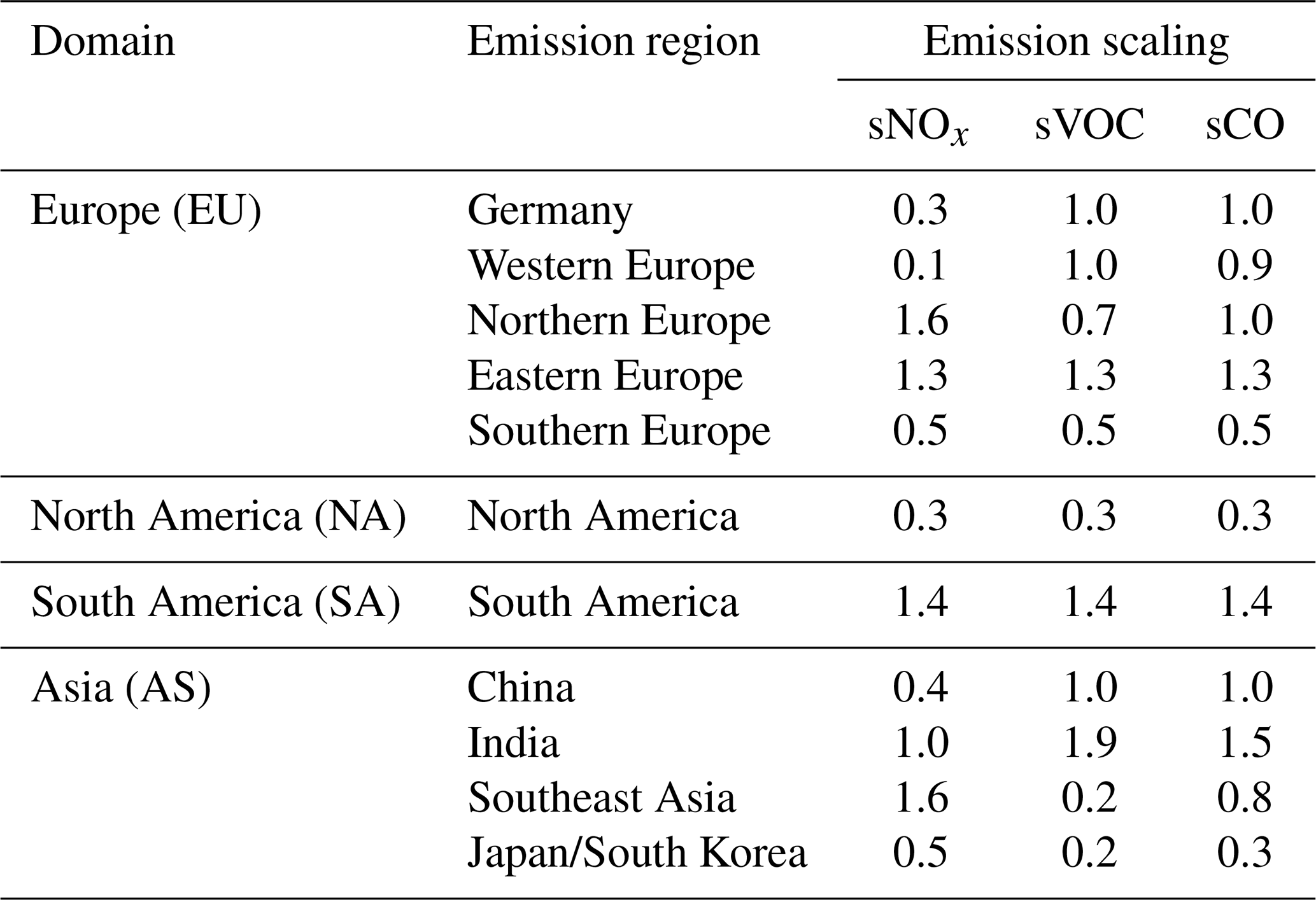
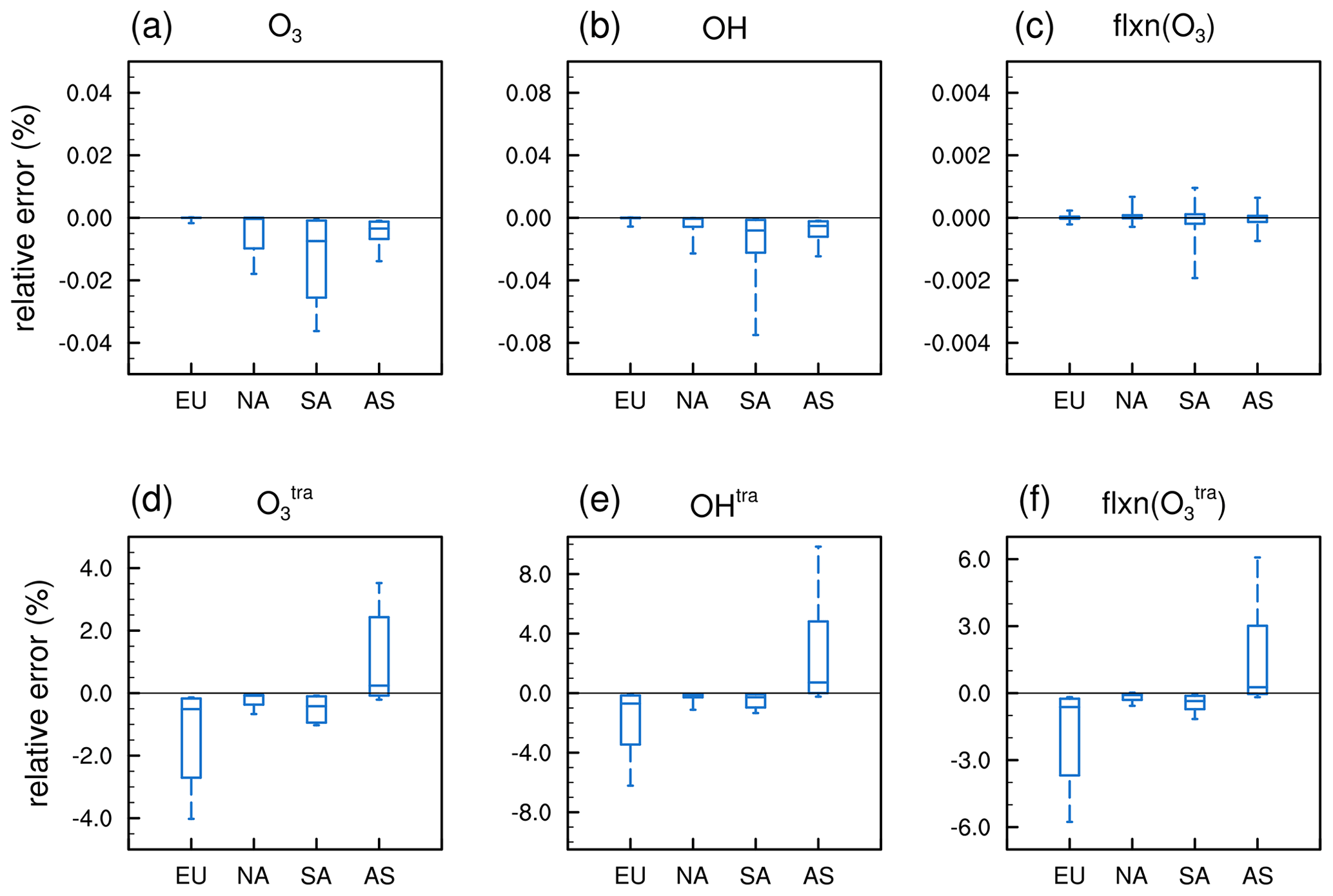
Figure 6Box plot of the relative errors between the simulations performed with TransClim and EMAC for the domains Europe (EU), North America (NA), South America (SA) and Asia (AS). The whiskers show the 5th and 95th percentiles. The relative errors for the variables O3 (a), OH (b) and flxn(O3) (c) as well as the contributions (d), OHtra (e) and flxn(O) (f) are shown. For O3 and , the relative errors of the tropospheric columns are shown. For OH and OHtra, the deviations of the tropospheric means are displayed. For flxn(O3) and flxn(O), the values at the top of the atmosphere are taken into account.
Moreover, TransClim is evaluated for different strengths of emission scaling in one emission region. For the emission region North America, the road traffic emissions of NOx, VOC and CO are scaled simultaneously by 0.3, 0.75, 1.5 and 1.8. Again, simulations with TransClim and EMAC are performed with the chosen emission scaling factors and the resulting relative errors are displayed in Fig. 7. Overall, the errors are very low. The contributions O, OHtra and flxn(O) show larger errors but still do not exceed 4 %. The simulation with the scaling factor 1.5 has larger deviations for all regarded variables than the simulations with the scaling factors 0.3, 0.75 and 1.8. This is not surprising as the current LUT used for TransClim contains EMAC simulations with all road traffic emissions in North America set to 0, 0.5, 12 and 2. The closer the chosen emission scaling factors are to these interpolation points in the LUT, the better the results determined by TransClim are.
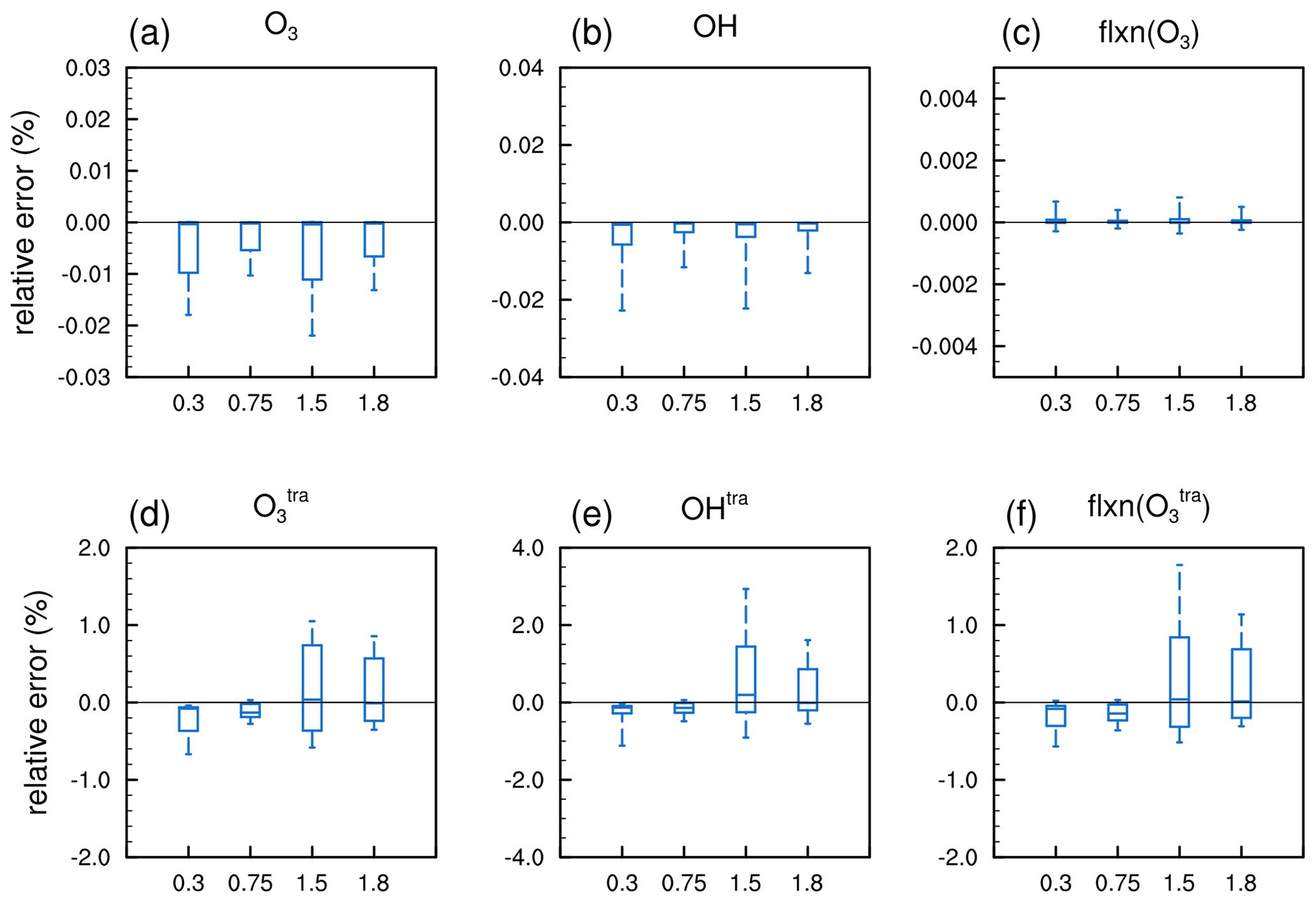
Figure 7Box plot of the relative errors between the simulations performed with TransClim and EMAC for different emission scalings. The road traffic emissions in North America are scaling with 0.3, 0.75, 1.5 and 1.8. The whiskers show the 5th and 95th percentiles. The relative errors for the variables O3 (a), OH (b) and flxn(O3) (c) as well as the contributions (d), OHtra (e) and flxn(O) (f) are shown. For O3 and , the relative errors of the tropospheric columns are shown. For OH and OHtra, the deviations of the tropospheric means are displayed. For flxn(O3) and flxn(O), the values at the top of the atmosphere are taken into account.
Summing up, these evaluation simulations show that TransClim reproduces the results obtained by EMAC very well. Road traffic emission variations in different parts of the world reveal deviations less than 10 %. For different strengths of emission variations in one emission region, the deviations are even lower (below 4 %). Thus, TransClim is able to reliably assess the climate effect of road traffic emission variations between 0 % and 200 % over different parts of the world.
3.2 Comparison with VEU1 simulations
In this section, EMAC simulations performed within the project VEU1 are reproduced with TransClim to assess the performance of TransClim. The DLR project VEU1 (Verkehrsentwicklung und Umwelt 1, i.e. Transport and the Environment 1, Henning et al. (2015), https://verkehrsforschung.dlr.de/projekte/veu, last access: 20 July 2022) examined German transport and its effect on the environment (Hendricks et al., 2018). In VEU1, EMAC simulations were performed to quantify the climate impact of future road traffic emission scenarios. Road traffic emissions for the year 2030 were determined and their impact on NOx, O3 and OH was computed with EMAC. This offers a good opportunity to test the performance of TransClim.
Within the scope of the project VEU1, German road traffic emissions were derived for present-day conditions as well as for possible future scenarios. The transport demand was determined based on socio-economic data such as population, households, income levels, economic development and demographic trends. To compute the road traffic emissions, the influence of railways and inland shipping, as well as passenger and freight transport, was regarded. For passenger transport, different transport modes such as motorized private transport, public transport, bicycles and pedestrians were taken into account. Additionally, different vehicle and fuel types as well as the emission classes were considered. The development of new technologies in the transport sectors was modelled as well. Considering all these different factors, an emission scenario for German road traffic emissions for the years 2008, 2020 and 2030 was created.
In VEU1, the climate impact of this emission scenario was simulated with EMAC only for the year 2030 using the perturbation method. This method compares two EMAC simulations: one simulation contains all emissions, and another simulation neglects the road traffic emissions. For these simulations, Hendricks et al. (2018) also use the QCTM mode of EMAC (see Sect. 2.4.1), which significantly reduces the numerical noise of a chemical perturbation. However, it may still be challenging to quantify the climate effect of a small perturbation. Hence, in order to obtain a robust signal of the German road traffic emissions, the perturbation signal was enhanced. Thus, not only the road traffic emissions in Germany, but also the road traffic emissions in all European countries were set to zero. This method determines the climate impact of the European road traffic emissions. Subsequently, to estimate the O3 radiative forcing of the German traffic emissions, the resulting European radiative forcing from the change in O3 was in turn downscaled according to the ratio of German to European traffic emissions of NOx. However, German road traffic emissions influence not only the tropospheric ozone, but also the lifetime of methane. To further quantify the effect of German road traffic, the CH4 lifetime change caused by German road traffic emissions was deduced from the OH change of the EMAC simulation. More details on the specific model setup of the EMAC simulations are found in Gottschaldt et al. (2013) and Hendricks et al. (2018).
The results obtained by the project VEU1 offer the opportunity to evaluate TransClim with respect to the climate impact of O3 and CH4 lifetime change caused by regional transport emissions. TransClim considers the German road traffic emissions for the years 2008, 2020 and 2030 and the European emission inventory for the year 2030 developed in VEU1. Subsequently, it is used to reproduce the results from the EMAC simulations performed in VEU1. The emission scaling factors (factors by which the reference emissions are scaled) for TransClim are presented in Table 4. For this simulation, the resulting NOx (sum of NO and NO2) and OH mixing ratios are also computed by TransClim.
Table 4Emission scaling factors for the TransClim simulation to reproduce the VEU1 simulations with EMAC. The emission scaling factors in Germany for the years 2008, 2020 and 2030 are also indicated. For the remaining European regions, the emission scaling factors are set constant for the years 2008, 2020 and 2030. The scaling factors of the remaining emission regions are not listed in the table as they are kept at 1.

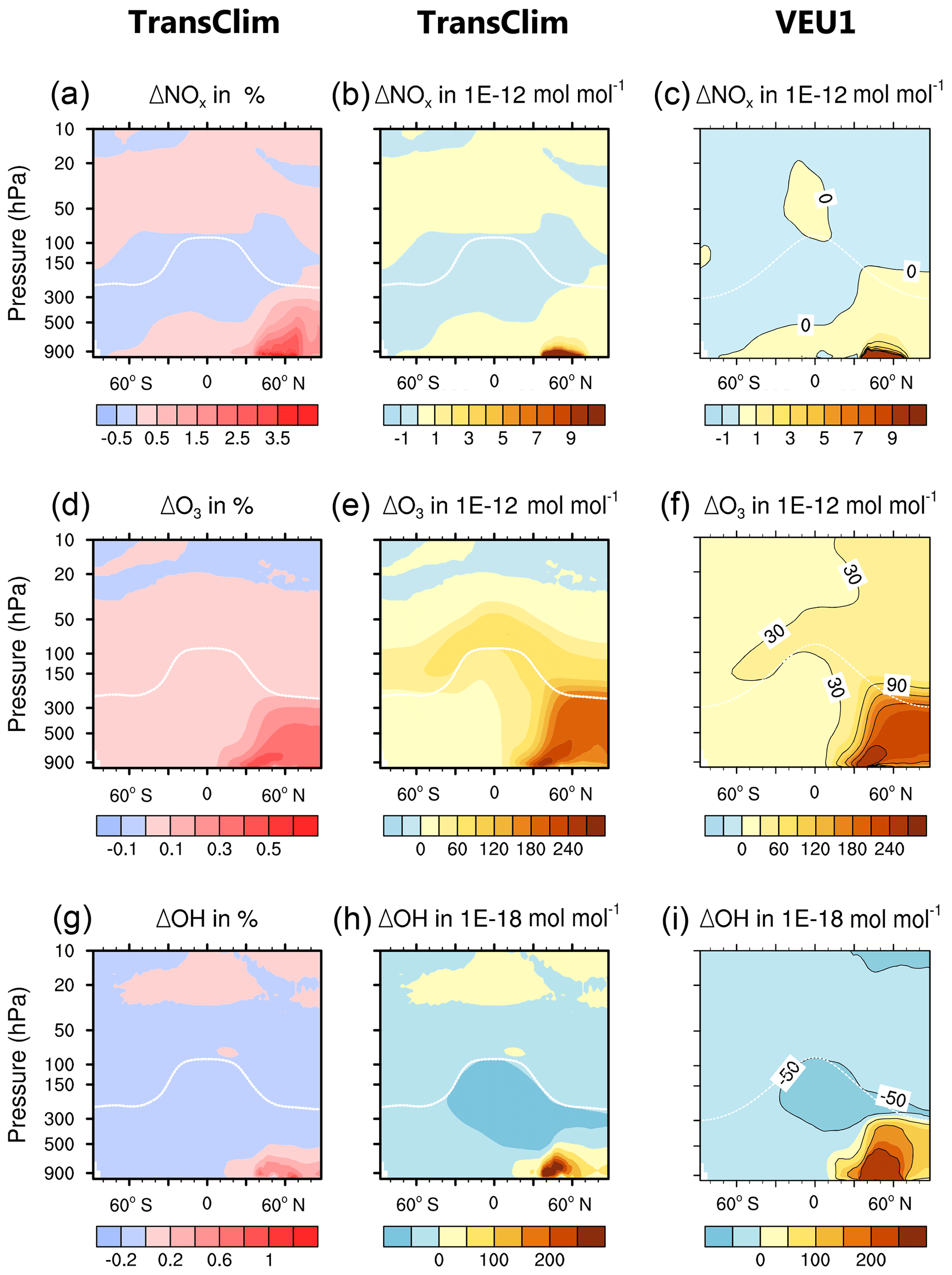
Figure 8Zonal mean of relative and absolute NOx, O3 and OH change caused by European road traffic emissions for the year 2030. Simulations performed with TransClim and EMAC (conducted within VEU1) are compared. The first and second column show the relative and absolute changes simulated with TransClim. The third column shows the absolute changes simulated with EMAC (taken from Fig. 6 in Hendricks et al., 2018). The white line indicates the tropopause.
The change in the zonal means of NOx, O3 and OH caused by the European road traffic emissions (i.e. difference between the reference simulation and “no European road traffic” simulation) for the year 2030 is shown in Fig. 8. The first and second column show the relative and absolute change derived from TransClim. The third column presents the absolute changes obtained with EMAC in VEU1 (Hendricks et al., 2018). European road traffic emissions increase NOx over the Northern Hemisphere. The increase (up to 4 %) is very confined to the latitudes where the European road traffic emissions occur. Furthermore, European road traffic emissions increase O3 in the Northern Hemisphere. The O3 rise is not only bound to the lower troposphere, but also reaches high up to the tropopause region. It even stretches into the lower stratosphere where O3 from European road traffic emissions is transported over the tropics. The zonal mean is increased by up to 0.5 % in the northern lower troposphere. Moreover, European road traffic emissions cause an OH increase in the lower troposphere, which is rather confined to the emission region. Furthermore, OH is decreased in the upper troposphere. TransClim reproduces the patterns of NOx and O3 increases very well compared to the EMAC simulation in VEU1. However, TransClim underestimates the OH increase caused by European road traffic emissions. In VEU1, the OH increase reaches the tropopause region in the Northern Hemisphere. In contrast, TransClim confines the OH increase below 500 hPa. In VEU1, a different emission inventory is used than for TransClim. As the OH chemistry is very sensitive to emissions, this can lead to different OH mixing ratios in VEU1 than the ones obtained by TransClim.
The results of VEU1 simulations in Fig. 8 are averaged over 3 years (2001 to 2003 considering the road traffic emissions of 2030). In contrast, TransClim determines an 1-year-average of 2010. The good agreement between TransClim and VEU1 shows that the LUTs consisting of 1-year simulations are sufficiently good to describe the NOx, O3 and OH change derived from a 3-year simulation with EMAC.
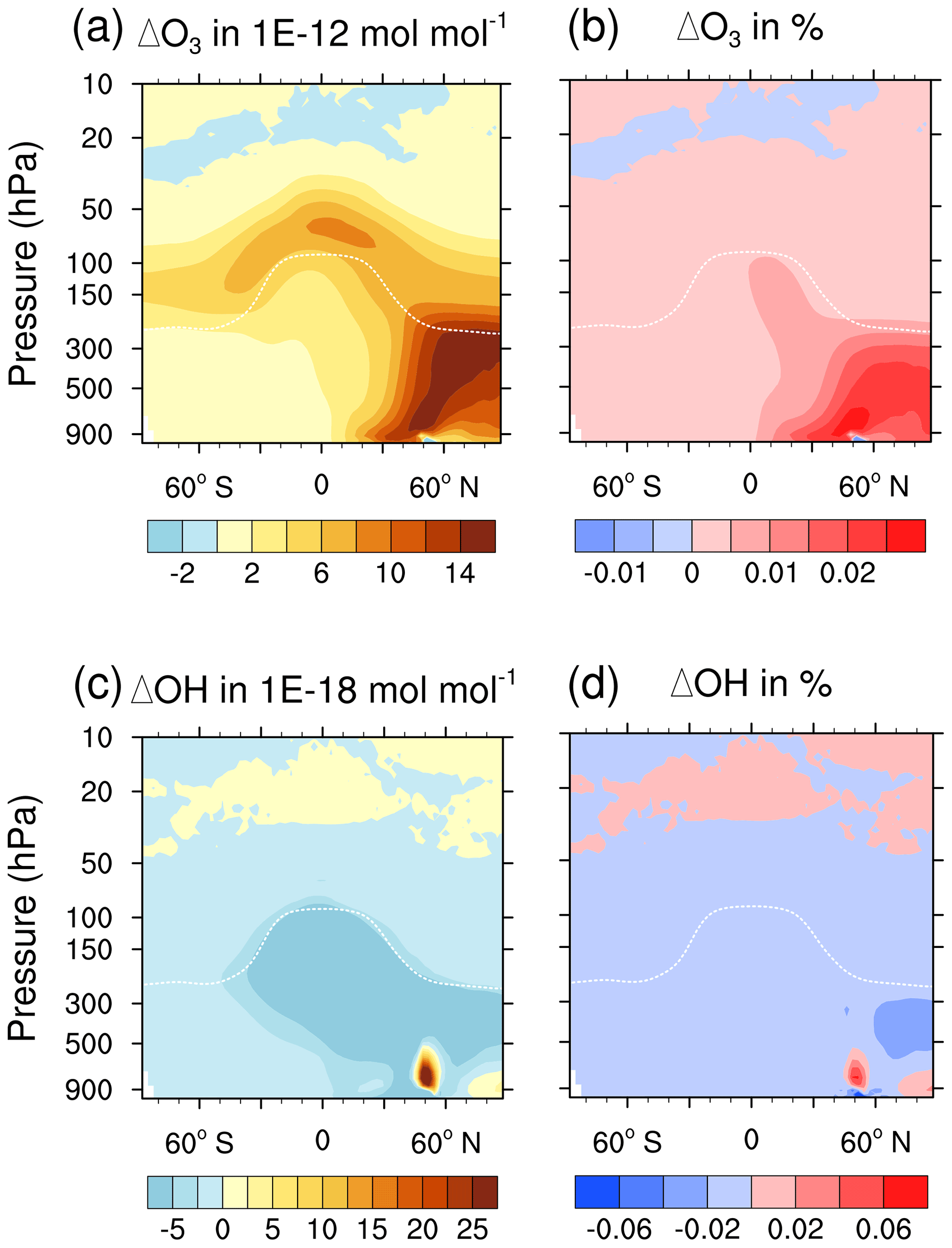
Figure 9Zonal mean of relative and absolute O3 and OH change caused by German road traffic emissions for the year 2030. The simulation is performed with TransClim. The white line indicates the tropopause.
TransClim also determines the O3 impact of only German road traffic emissions on climate without the requirement of scaling emissions to enhance the signal-to-noise ratio (see also Hendricks et al., 2018). An additional simulation with TransClim is performed in which all road traffic emissions in Germany are neglected. To obtain the climate impact of German road traffic emissions, the TransClim simulation without German road traffic emissions is subtracted from the reference simulation with all road traffic emissions (reference simulation − “no German road traffic emissions” simulation). The resulting O3 and OH changes are shown in Fig. 9. The pattern of the O3 increase is very similar to the O3 change caused by the European road traffic emissions (Fig. 8). But the magnitude of the O3 change is smaller for German as for European road traffic emissions as the amount of road traffic emissions released by Germany is smaller. The zonal mean of O3 rises by up to 0.03 % in the lower troposphere of the Northern Hemisphere. Noteworthy is the fact that a small O3 decrease is observed in the lowermost atmospheric layers at 50∘ N. In this region, German road traffic emissions significantly increase the NOx concentration by about 0.4 % (zonal average). The O3 decrease due to a NOx increase indicates that this region is VOC-limited. German road traffic emissions further decrease the OH concentration in the free troposphere. However, a small increase of up to 0.06 % is observed in the lower troposphere at 50∘ N.
Table 5Ozone radiative forcing (RF(O3)) and CH4 lifetime () change for the simulations derived in VEU1 (Hendricks et al., 2018) and computed by TransClim for the year 2030. The column “Europe” shows the results for the European road traffic emissions, and the column “Germany” describes the values for the German road traffic emissions.
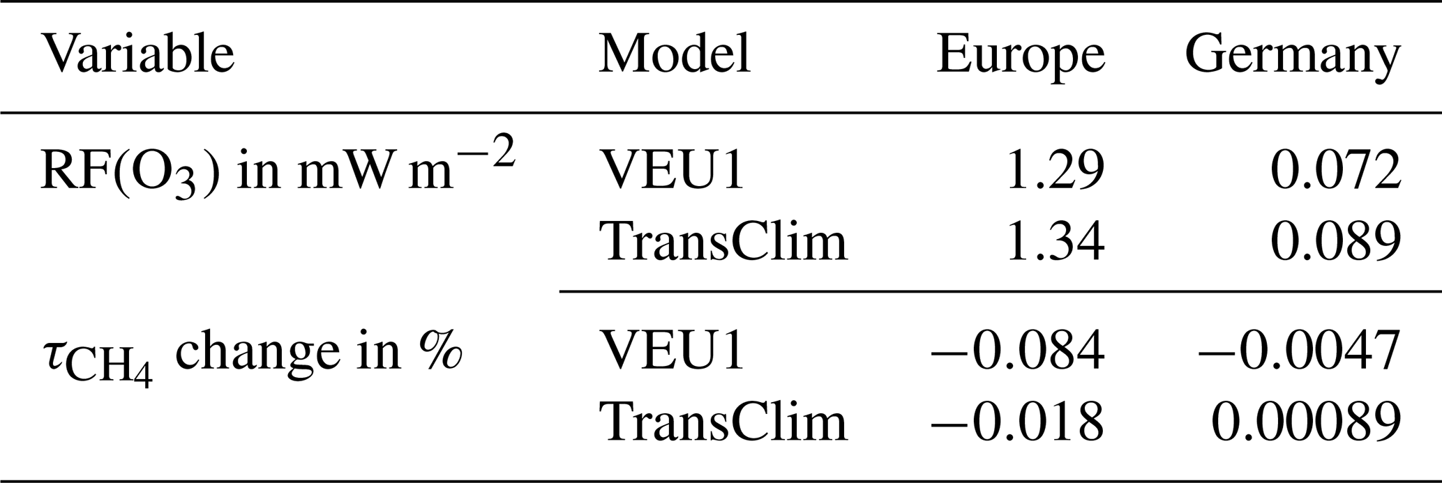
The O3 radiative forcings and the change in CH4 lifetime for the year 2030 are derived from the TransClim simulation and compared with the VEU1 results in Table 5. TransClim determines an O3 radiative forcing caused by European road traffic emissions of 1.34 mW m−2, which deviates by only 4 % from the VEU1 value. The O3 forcing for the German road traffic emissions is 0.089 mW m−2 (derived with TransClim). It differs from the value obtained in VEU1 by 24 %. This is not surprising as in VEU1 the German values are determined by downscaling the forcing from the European road traffic emissions (see above). For the change in CH4 lifetime caused by European road traffic emissions, TransClim obtains a significantly lower value than VEU1. On the one hand, the OH increase obtained by TransClim is smaller than in VEU1 (compare to Fig. 8). On the other hand, the CH4 lifetimes of the simulations for TransClim's LUTs (about 7.7 years) are generally lower than of the EMAC simulations used for VEU1 (about 8.5 years). This can be caused by the different emission inventories used for TransClim and VEU1 simulations. Moreover, different methods for calculating the CH4 lifetime can cause different CH4 lifetimes and thus influence variations in CH4 lifetimes (Lawrence et al., 2001). Interestingly, the CH4 lifetime change due to European road traffic emissions is negative. But for German road traffic emissions, TransClim computes a positive lifetime change. This change in sign is caused by the fact that European road traffic emissions increase the tropospheric mean OH by 0.03 %, but German road traffic emissions decrease the tropospheric mean OH by 0.003 %. Due to downscaling the CH4 lifetime change caused by European traffic emissions to obtain the lifetime change caused by German traffic emissions in VEU1, a change in sign can not be reproduced. As Germany lies in Central Europe, it is more dominated by high background NOx concentrations than the whole domain Europe. This could be a possible reason for the discrepancy between the German and European OH change. For high NOx concentrations, the reaction between OH and NO2 becomes more and more important, decreasing the OH concentration (Hoor et al., 2009).
Table 6Radiative forcing of ozone change (O3) and contribution change () in mW m−2 due to German road traffic emissions for the years 2008, 2020, 2030. The results for the VEU1 simulations with EMAC (Hendricks et al., 2018) and TransClim are given.
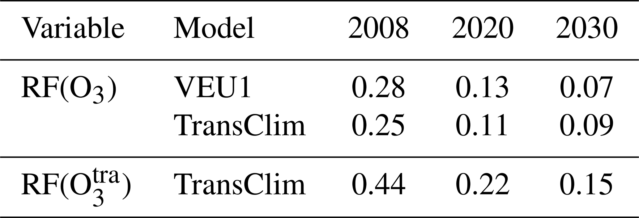
To estimate the O3 radiative forcing for different years in VEU1, Hendricks et al. (2018) scaled the O3 radiative forcing with the NOx emissions from road traffic. Using the emission scaling factors of Table 4, TransClim also computes the O3 radiative forcings for these years. Table 6 presents the O3 radiative forcing estimated from the VEU1 simulations and from TransClim. The O3 radiative forcing obtained by VEU1 decreases in future. This decreasing trend is reproduced well by TransClim. However, the values differ by 0.02 mW m−2. TransClim obtains lower forcings for 2008 and 2020 and a larger forcing for 2030. The radiative forcing of the contribution of German road traffic emissions to the ozone concentration (RF()) obtained by TransClim is also given in Table 6. It is about twice as large as the radiative forcing due to total O3 change caused by German road traffic emissions (RF(O3)). This indicates that the effect of German road traffic emissions on the radiative forcing is underestimated by a factor of 2 when only the total O3 mixing ratios and not the O3 contributions are regarded (in agreement with Mertens et al., 2018).
Summing up, TransClim reproduces the results obtained by EMAC very well. Although TransClim underestimates the results of EMAC slightly, it performs well when being directly compared to EMAC (deviations are below 10 %). It also reproduces the EMAC simulations performed in VEU1 satisfactorily well. Moreover, the overall pattern of European road traffic emissions is described very well by TransClim. Only OH mixing ratios are smaller, leading to a lower CH4 lifetime change.
As shown above, TransClim efficiently determines the O3 effect of road traffic emission scenarios on climate. The algorithm used in TransClim (see Sect. 2.5) reproduces the results obtained with the global chemistry–climate model EMAC very well.
TransClim considers the emission species NOx, VOC and CO and computes the mixing ratios of O3 and O in the atmosphere. Thus, the algorithm fulfils objective (1) of Sect. 2.3. By interpolating within the LUTs, the non-linearity of the tropospheric O3 chemistry is regarded (objective 2). Furthermore, the road traffic emissions are split up into 11 emission regions. LUTs are set up for each emission region. Hence, the effect of different emission regions is included in the algorithm (objective 3). As TransClim sets up a LUT for each grid box of an EMAC simulation, it can determine the pattern of a variable change. Consequently, TransClim calculates not only the global and tropospheric means, but also the regional effect caused by an emission scenario (objective 4). Moreover, the method is not only applicable for the determination of O3 and , but also for other variables such as OH and OHtra as well as the radiative forcings of O3 and road traffic (objective 5).
The algorithm used in TransClim determines the climate effect of an emission scenario efficiently (objective 6). For example, to compute the changes in the global mean O3 concentration of an emission scenario in one emission region, TransClim needs 0.2 s. Calculating the three-dimensional O3 field for one emission region, it takes up to 15 min on a standard computer. For the determination of the total variables such as O3, OH and flxn(O3), the algorithm obtains very good results: the computed values deviate only little from the values obtained by EMAC (below 1 %; see Sect. 3.1). The results of the contributions of road traffic emissions such as O, OHtra and flxn(O) deviate larger (less than 10 %). But the deviations are still so small that they do not restrict the application of TransClim. Overall, TransClim fulfils all objectives of Sect. 2.3 and thus performs very well.
The response model TransClim efficiently quantifies the O3 effect of road traffic emission scenarios on climate. Considering the road traffic emission species NOx, VOC and CO, TransClim computes the change in atmospheric variables such as O3, OH and NOx as well as the stratosphere-adjusted radiative forcing of O3. TransClim is based on lookup tables which contain precalculated relationships of emissions and their climate effect. These relationships are simulated by the global chemistry–climate model EMAC. Road traffic emissions are divided into 11 emission regions (Germany, Western Europe, Northern Europe, Eastern Europe, Southern Europe, North America, South America, China, India, Southeast Asia and Japan/South Korea). TransClim is able to consider emission scenarios in which road traffic emissions of NOx, VOC and CO are varied from 0 % to 200 % in each emission region.
The algorithm used in TransClim is able to compute the climate effect of road traffic emission scenarios very fast. Running on a standard computer, TransClim is about 6000 times faster than the global chemistry–climate model EMAC running on a high-performance computer. For example, it takes 0.2 s to calculate the global mean climate response of an emission scenario. In other words, TransClim needs approximately 4.5×10⁵ less computing time than a climate simulation with EMAC. Hence, it offers a suitable tool for assessing a broad range of road traffic emission scenarios. As TransClim further considers the tagging method, it allows for calculating not only the changes in atmospheric composition, but also the contribution of road traffic emissions.
The comparison of TransClim simulations with EMAC simulations (which have not been used for the training to set up TransClim) shows that TransClim is able to reproduce the changes in chemical species and in radiative fluxes very well. The comparison of TransClim with equivalent EMAC simulations reveals that the errors are small (0.01 %–10 %) and thus do not hamper the application of TransClim.
However, the current setup of TransClim restricts its range of usage. The LUTs are generated from emission variation simulations with the global model EMAC. This allows the determination of the atmospheric response on a global and regional scale. The algorithm used in TransClim is also able to assess the effect of road traffic emissions on surface ozone and air quality. But to calculate the atmospheric response on a local scale, it is mandatory to perform additional simulations with models such as the climate model MECO(n) (coupled model system MESSyfied ECHAM and COSMO models nested n-times; Kerkweg and Jöckel, 2012a, b) which can have a finer grid resolution (0.44∘). Furthermore, the LUTs are based on emission variation simulations of the year 2010 and thus are bound to specific O3 background concentrations, emissions and meteorology. For example, varying the road traffic emissions for different O3 backgrounds in a future climate may result in a completely different O3 change. Thus, the current set of LUTs would not be valid any more. New LUTs need to be created considering the climate response of a very different O3 background concentration. Moreover, the current LUTs only consider variations of road traffic emissions. To include the O3 response of other land-based traffic modes such as railways and shipping, additional emission variation simulations are required to generate new LUTs.
Overall, the approach used for TransClim is very flexible. The LUTs can be easily extended to include additional traffic modes, emissions regions and years. However, the computational resources required for emission variation simulations are high and hamper the extension of the LUTs. But once the LUTs are generated, TransClim is able to quickly compute the O3 effect of an emission scenario on climate.
The impact of traffic emissions on air quality and climate is also examined by other response models. For example, the response models LinClim and AirClim analyse the climate response of aviation emissions (Lim et al., 2007; Grewe and Stenke, 2008; Grewe et al., 2012; Dahlmann et al., 2016). Both models use a linear approach to compute the O3 change in the stratosphere. In comparison to the lower troposphere, the O3 chemistry in the upper troposphere and stratosphere is not dominated by strong non-linearities. Thus, the linear approach for determining the O3 concentration in the stratosphere works well for LinClim and AirClim. However, these approaches would not work for TransClim as the road traffic emissions are released into the lower troposphere where the non-linearities of the O3 chemistry are an important factor to be considered.
The study by Wild et al. (2012) presents a parametrization to quantify surface ozone changes caused by precursor emission variations of NOx, CO, VOC and CH4, including the non-linear behaviour of the tropospheric ozone chemistry. But their approach only considers the non-linear relationship between ozone change and NOx emissions. This parametrization works well for NOx emission changes of up to 60 %. But it remains insufficient for higher NOx emission reduction, leading to errors of up to 5 ppb for O3 changes over Europe. Moreover, Wild et al. (2012) regard the influence of the precursors NOx, CO and VOC on O3 separately, which leads to errors of up to 7 % for 20 % emission reductions when compared to the combined emission reduction of the three precursors. In comparison to Wild et al. (2012), TransClim regards the non-linear relationship in O3 production as well as the combination of emission changes for all three precursors NOx, VOC and CO. Furthermore, it works well for large emission changes between 0 % and 200 % (errors below 4 %).
Another example is the response model TM5-FASST. It investigates the impact of pollutants such as NOx, SO2, CO and BC on air quality (Van Dingenen et al., 2018). Moreover, TM5-FASST calculates radiative forcings, temperature variations, mortality and the impact on vegetation and crop yield. But this response model uses a linear approach for computing the O3 change. In particular for a doubling of NOx emissions, this results in high deviations for summer surface ozone (over 41 %). Furthermore, TM5-FASST considers the influence of the precursors NOx, VOC and CO on the O3 chemistry separately. As TransClim interpolates within the LUTs which are based on NOx, VOC and CO emissions simultaneously, it considers the influence of the three precursors in producing O3 together. In this manner, TransClim regards the non-linearity of the tropospheric O3 chemistry. Even though TM5-FASST determines more impact metrics, it does not regard the contribution of emission sectors to the O3 concentration by using a tagging method. Thus so far, no other response model than TransClim is able to analyse the climate impact as well as the contribution of road traffic emissions together.
Summing up, TransClim is able to quantify the climate effect of O3 changes caused by road traffic emission scenarios. However, further developments are planned. To assess the climate effect of future emission scenarios, the impact of different O3 background concentrations needs to be included in TransClim. Moreover, the radiative forcing caused by a change of methane lifetime will be embedded in TransClim as well. To further expand the applicability of TransClim, the integration of other traffic modes such as shipping is desirable. The current implementation regards only the climate metric stratosphere-adjusted radiative forcing. To provide deeper insight into the climate effect, further climate metrics such as surface temperature change need to be integrated. In addition, road traffic emissions also affect aerosols. The inclusion of the aerosol effect in TransClim would complete the assessment of mitigation strategies.
Despite these planned extensions of TransClim, the response model is operational and ready to assess the O3 effect of mitigation options for road traffic on climate.
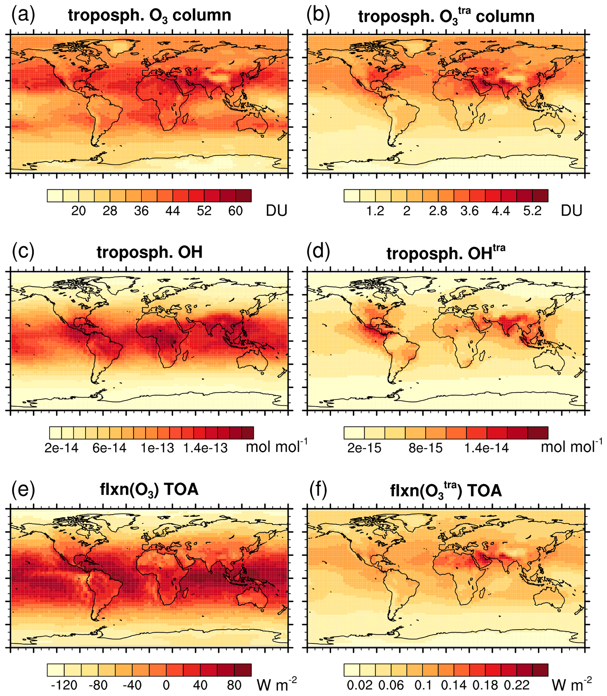
Figure A1Ozone (O3), hydroxyl radical (OH) and ozone net radiative fluxes (flxn(O3)) as well as the contribution to ozone (), to hydroxyl radical (OHtra) and to ozone net radiative fluxes (flxn(O)) determined by TransClim for the simulation “Europe”. The emission scaling factors are given in Table 3. The tropospheric columns of O3 and are given in Dobson units (DU) (a, b). For OH and OHtra, the tropospheric means are shown (c, d). The values at the top of the atmosphere (TOA) are displayed for flxn(O3) and flxn(O) (e, f).
The exact version of the model TransClim used to produce the results presented in this paper is archived at the German Climate Computing Center DKRZ: https://doi.org/10.35089/WDCC/TransClim_v01_chem-cl_response (Rieger and Grewe, 2021). The global and tropospheric mean values of the EMAC simulations for the lookup tables are stored at https://doi.org/10.26050/WDCC/Lookup-tables_for_TransClim (Rieger and Grewe, 2022).
The supplement related to this article is available online at: https://doi.org/10.5194/gmd-15-5883-2022-supplement.
VSR designed the model concept, implemented the model, performed the simulations and evaluations and wrote the paper. VG conceived the model concept, coordinated its development and significantly contributed to the interpretation of the results and to the text.
At least one of the (co-)authors is a member of the editorial board of Geoscientific Model Development. The peer-review process was conducted by an independent editor, and the authors also have no other competing interests to declare.
Publisher’s note: Copernicus Publications remains neutral with regard to jurisdictional claims in published maps and institutional affiliations.
This study was supported by the DLR transport program (project “Transport and the Environment – VEU2”). The EMAC simulations were performed at the German Climate Computing Center (DKRZ, Hamburg, Germany), which also provided kind support for long-term storage of the model output analysed in this work. We used the NCAR Command Language (NCL) for data analysis and to create the figures of this study. NCL is developed by UCAR/NCAR/CISL/TDD and available online at https://doi.org/10.5065/D6WD3XH5. We thank Axel Lauer from DLR and two anonymous reviewers for very helpful comments which improved the article.
The article processing charges for this open-access publication were covered by the German Aerospace Center (DLR).
This paper was edited by Olaf Morgenstern and reviewed by two anonymous referees.
Dahlmann, K., Grewe, V., Frömming, C., and Burkhardt, U.: Can we reliably assess climate mitigation options for air traffic scenarios despite large uncertainties in atmospheric processes?, Transport. Res. D: Tr. E., 46, 40–55, https://doi.org/10.1016/j.trd.2016.03.006, 2016. a
Deckert, R., Jöckel, P., Grewe, V., Gottschaldt, K.-D., and Hoor, P.: A quasi chemistry-transport model mode for EMAC, Geosci. Model Dev., 4, 195–206, https://doi.org/10.5194/gmd-4-195-2011, 2011. a
Dietmüller, S., Jöckel, P., Tost, H., Kunze, M., Gellhorn, C., Brinkop, S., Frömming, C., Ponater, M., Steil, B., Lauer, A., and Hendricks, J.: A new radiation infrastructure for the Modular Earth Submodel System (MESSy, based on version 2.51), Geosci. Model Dev., 9, 2209–2222, https://doi.org/10.5194/gmd-9-2209-2016, 2016. a
Dodge, M.: Combined use of modeling techniques and smog chamber data to derive ozoneprecursor relationships, in: International Conference on Photochemical Oxidant Pollution and its Control: Proceedings, edited by: Dimitriades, B., U.S. Environmental Protection Agency, Environmental Sciences Research Laboratory, Research Triangle Park, N.C., Vol. II., 881–889, ePA/600/3-77-001b, 1977. a
Fouquart, Y. and Bonnel, B.: Computations of solar heating of the Earth's atmosphere: A new parameterization, Beitr. Phys. Atmos., 53, 35–62, 1980. a
Fowler, D., Amann, M., Anderson, R., Ashmore, M., Cox, P., Depledge, M., Derwent, D., Grennfelt, P., Hewitt, N., Jenkin, M., Kelly, F., Liss, P., Pilling, M., Pyle, J., Slingo, J., and Stevenson, D.: Ground-level ozone in the 21st century: future trends, impacts and policy implications, Science Policy, The Royal Society, ISBN 9780854037131, 2008. a
Fuglestvedt, J., Berntsen, T., Myhre, G., Rypdal, K., and Skeie, R. B.: Climate forcing from the transport sectors, P. Natl. Acad. Sci., 105, 454–458, https://doi.org/10.1073/pnas.0702958104, 2008. a
Gottschaldt, K., Voigt, C., Jöckel, P., Righi, M., Deckert, R., and Dietmüller, S.: Global sensitivity of aviation NOx effects to the HNO3-forming channel of the HO2 + NO reaction, Atmos. Chem. Phys., 13, 3003–3025, https://doi.org/10.5194/acp-13-3003-2013, 2013. a
Granier, C. and Brasseur, G. P.: The impact of road traffic on global tropospheric ozone, Geophys. Res. Lett., 30, 1086, https://doi.org/10.1029/2002GL015972, 2003. a
Granier, C., Bessagnet, B., Bond, T., D'Angiola, A., Denier van der Gon, H., Frost, G. J., Heil, A., Kaiser, J. W., Kinne, S., Klimont, Z., Kloster, S., Lamarque, J.-F., Liousse, C., Masui, T., Meleux, F., Mieville, A., Ohara, T., Raut, J.-C., Riahi, K., Schultz, M. G., Smith, S. J., Thompson, A., van Aardenne, J., van der Werf, G. R., and van Vuuren, D. P.: Evolution of anthropogenic and biomass burning emissions of air pollutants at global and regional scales during the 1980–2010 period, Clim. Change, 109, 163, https://doi.org/10.1007/s10584-011-0154-1, 2011. a, b, c
Grewe, V.: A generalized tagging method, Geosci. Model Dev., 6, 247–253, https://doi.org/10.5194/gmd-6-247-2013, 2013. a
Grewe, V. and Stenke, A.: AirClim: an efficient tool for climate evaluation of aircraft technology, Atmos. Chem. Phys., 8, 4621–4639, https://doi.org/10.5194/acp-8-4621-2008, 2008. a
Grewe, V., Brunner, D., Dameris, M., Grenfell, J., Hein, R., Shindell, D., and Staehelin, J.: Origin and variability of upper tropospheric nitrogen oxides and ozone at northern mid-latitudes, Atmos. Environ., 35, 3421–3433, https://doi.org/10.1016/S1352-2310(01)00134-0, 2001. a
Grewe, V., Tsati, E., and Hoor, P.: On the attribution of contributions of atmospheric trace gases to emissions in atmospheric model applications, Geosci. Model Dev., 3, 487–499, https://doi.org/10.5194/gmd-3-487-2010, 2010. a, b, c, d, e, f
Grewe, V., Dahlmann, K., Matthes, S., and Steinbrecht, W.: Attributing ozone to NOx emissions: Implications for climate mitigation measures, Atmos. Environ., 59, 102–107, https://doi.org/10.1016/j.atmosenv.2012.05.002, 2012. a
Grewe, V., Tsati, E., Mertens, M., Frömming, C., and Jöckel, P.: Contribution of emissions to concentrations: the TAGGING 1.0 submodel based on the Modular Earth Submodel System (MESSy 2.52), Geosci. Model Dev., 10, 2615–2633, https://doi.org/10.5194/gmd-10-2615-2017, 2017. a, b
Guenther, A., Hewitt, C. N., Erickson, D., Fall, R., Geron, C., Graedel, T., Harley, P., Klinger, L., Lerdau, M., Mckay, W. A., Pierce, T., Scholes, B., Steinbrecher, R., Tallamraju, R., Taylor, J., and Zimmerman, P.: A global model of natural volatile organic compound emissions, J. Geophys. Res.-Atmos., 100, 8873–8892, https://doi.org/10.1029/94JD02950, 1995. a
Hendricks, J., Righi, M., Dahlmann, K., Gottschaldt, K.-D., Grewe, V., Ponater, M., Sausen, R., Heinrichs, D., Winkler, C., Wolfermann, A., Kampffmeyer, T., Friedrich, R., Klötzke, M., and Kugler, U.: Quantifying the climate impact of emissions from land-based transport in Germany, Transport. Res. D: Tr. E., 65, 825–845, https://doi.org/10.1016/j.trd.2017.06.003, 2018. a, b, c, d, e, f, g, h, i, j, k
Henning, A., Plohr, M., Özdemir, E., Hepting, M., Keimel, H., Sanok, S., Sausen, R., Pregger, T., Seum, S., Heinrichs, M., Müller, S., Winkler, C., Neumann, T., Seeback, O., V., M., and B., V.: The DLR Transport and the Environment Project – Building competency for a sustainable mobility future, in: Proceedings of the 4th International Conference on Transport, Atmosphere and Climate (TAC-4), edited by: Sausen, R., Unterstrasser, S., and Blum, A., Deutsches Zentrum für Luft- und Raumfahrt, Institut für Physik der Atmosphäre, Oberpfaffenhofen, 192–198, ISSN 0939-2963, 2015. a
Hoor, P., Borken-Kleefeld, J., Caro, D., Dessens, O., Endresen, O., Gauss, M., Grewe, V., Hauglustaine, D., Isaksen, I. S. A., Jöckel, P., Lelieveld, J., Myhre, G., Meijer, E., Olivie, D., Prather, M., Schnadt Poberaj, C., Shine, K. P., Staehelin, J., Tang, Q., van Aardenne, J., van Velthoven, P., and Sausen, R.: The impact of traffic emissions on atmospheric ozone and OH: results from QUANTIFY, Atmos. Chem. Phys., 9, 3113–3136, https://doi.org/10.5194/acp-9-3113-2009, 2009. a, b, c, d, e
Jedynska, A., Tromp, P. C., Houtzager, M. M., and Kooter, I. M.: Chemical characterization of biofuel exhaust emissions, Atmos. Environ., 116, 172–182, https://doi.org/10.1016/j.atmosenv.2015.06.035, 2015. a
Jöckel, P., Kerkweg, A., Pozzer, A., Sander, R., Tost, H., Riede, H., Baumgaertner, A., Gromov, S., and Kern, B.: Development cycle 2 of the Modular Earth Submodel System (MESSy2), Geosci. Model Dev., 3, 717–752, https://doi.org/10.5194/gmd-3-717-2010, 2010. a, b
Jöckel, P., Tost, H., Pozzer, A., Kunze, M., Kirner, O., Brenninkmeijer, C. A. M., Brinkop, S., Cai, D. S., Dyroff, C., Eckstein, J., Frank, F., Garny, H., Gottschaldt, K.-D., Graf, P., Grewe, V., Kerkweg, A., Kern, B., Matthes, S., Mertens, M., Meul, S., Neumaier, M., Nützel, M., Oberländer-Hayn, S., Ruhnke, R., Runde, T., Sander, R., Scharffe, D., and Zahn, A.: Earth System Chemistry integrated Modelling (ESCiMo) with the Modular Earth Submodel System (MESSy) version 2.51, Geosci. Model Dev., 9, 1153–1200, https://doi.org/10.5194/gmd-9-1153-2016, 2016. a
Karavalakis, G., Durbin, T. D., Shrivastava, M., Zheng, Z., Villela, M., and Jung, H.: Impacts of ethanol fuel level on emissions of regulated and unregulated pollutants from a fleet of gasoline light-duty vehicles, Fuel, 93, 549–558, https://doi.org/10.1016/j.fuel.2011.09.021, 2012. a
Kerkweg, A. and Jöckel, P.: The 1-way on-line coupled atmospheric chemistry model system MECO(n) – Part 1: Description of the limited-area atmospheric chemistry model COSMO/MESSy, Geosci. Model Dev., 5, 87–110, https://doi.org/10.5194/gmd-5-87-2012, 2012a. a
Kerkweg, A. and Jöckel, P.: The 1-way on-line coupled atmospheric chemistry model system MECO(n) – Part 2: On-line coupling with the Multi-Model-Driver (MMD), Geosci. Model Dev., 5, 111–128, https://doi.org/10.5194/gmd-5-111-2012, 2012b. a
Kerkweg, A., Sander, R., Tost, H., and Jöckel, P.: Technical note: Implementation of prescribed (OFFLEM), calculated (ONLEM), and pseudo-emissions (TNUDGE) of chemical species in the Modular Earth Submodel System (MESSy), Atmos. Chem. Phys., 6, 3603–3609, https://doi.org/10.5194/acp-6-3603-2006, 2006. a
Lawrence, M. G., Jöckel, P., and von Kuhlmann, R.: What does the global mean OH concentration tell us?, Atmos. Chem. Phys., 1, 37–49, https://doi.org/10.5194/acp-1-37-2001, 2001. a
Lim, L., Lee, D. S., Sausen, R., and Ponater, M.: Quantifying the effects of aviation on radiative forcing and temperature with a climate response model, in: Proceedings of the TAC-Conference, 202–208, ISBN 9279045830, 2007. a
Matthes, S., Grewe, V., Sausen, R., and Roelofs, G.-J.: Global impact of road traffic emissions on tropospheric ozone, Atmos. Chem. Phys., 7, 1707–1718, https://doi.org/10.5194/acp-7-1707-2007, 2007. a
Mertens, M., Grewe, V., Rieger, V. S., and Jöckel, P.: Revisiting the contribution of land transport and shipping emissions to tropospheric ozone, Atmos. Chem. Phys., 18, 5567–5588, https://doi.org/10.5194/acp-18-5567-2018, 2018. a, b, c
Mertens, M., Kerkweg, A., Grewe, V., Jöckel, P., and Sausen, R.: Attributing ozone and its precursors to land transport emissions in Europe and Germany, Atmos. Chem. Phys., 20, 7843–7873, https://doi.org/10.5194/acp-20-7843-2020, 2020. a, b
Mills, G., Buse, A., Gimeno, B., Bermejo, V., Holland, M., Emberson, L., and Pleijel, H.: A synthesis of AOT40-based response functions and critical levels of ozone for agricultural and horticultural crops, Atmos. Environ., 41, 2630–2643, https://doi.org/10.1016/j.atmosenv.2006.11.016, 2007. a
Mlawer, E. J., Taubman, S. J., Brown, P. D., Iacono, M. J., and Clough, S. A.: Radiative transfer for inhomogeneous atmospheres: RRTM, a validated correlated-k model for the longwave, J. Geophys. Res.-Atmos., 102, 16663–16682, https://doi.org/10.1029/97JD00237, 1997. a
Niemeier, U., Granier, C., Kornblueh, L., Walters, S., and Brasseur, G. P.: Global impact of road traffic on atmospheric chemical composition and on ozone climate forcing, J. Geophys. Res.-Atmos., 111, d09301, https://doi.org/10.1029/2005JD006407, 2006. a
Nissen, K. M., Matthes, K., Langematz, U., and Mayer, B.: Towards a better representation of the solar cycle in general circulation models, Atmos. Chem. Phys., 7, 5391–5400, https://doi.org/10.5194/acp-7-5391-2007, 2007. a
Reis, S., Simpson, D., Friedrich, R., Jonson, J., Unger, S., and Obermeier, A.: Road traffic emissions – predictions of future contributions to regional ozone levels in Europe, Atmos. Environ., 34, 4701–4710, https://doi.org/10.1016/S1352-2310(00)00202-8, 2000. a
Rieger, V. S.: A new method to assess the climate effect of mitigation strategies in road traffic, PhD thesis, Delft University of Technology, https://doi.org/10.4233/uuid:cc96a7c7-1ec7-449a-84b0-2f9a342a5be5, 2018. a, b
Rieger, V. and Grewe, V.: Assessing the climate effect of mitigation strategies for road traffic: The chemistry-climate response model TransClim, World Data Center for Climate (WDCC) at DKRZ, WDCC [code], https://doi.org/10.35089/WDCC/TransClim_v01_chem-cl_response, 2021. a
Rieger, V. and Grewe, V.: Lookup-tables for TransClim, World Data Center for Climate (WDCC) at DKRZ, WDCC [data set] https://doi.org/10.26050/WDCC/Lookup-tables_for_TransClim, 2022. a
Rieger, V. S., Mertens, M., and Grewe, V.: An advanced method of contributing emissions to short-lived chemical species (OH and HO2): the TAGGING 1.1 submodel based on the Modular Earth Submodel System (MESSy 2.53), Geosci. Model Dev., 11, 2049–2066, https://doi.org/10.5194/gmd-11-2049-2018, 2018. a
Righi, M., Eyring, V., Gottschaldt, K.-D., Klinger, C., Frank, F., Jöckel, P., and Cionni, I.: Quantitative evaluation of ozone and selected climate parameters in a set of EMAC simulations, Geosci. Model Dev., 8, 733–768, https://doi.org/10.5194/gmd-8-733-2015, 2015. a
Roeckner, E., Brokopf, R., Esch, M., Giorgetta, M., Hagemann, S., Kornblueh, L., Manzini, E., Schlese, U., and Schulzweida, U.: Sensitivity of Simulated Climate to Horizontal and Vertical Resolution in the ECHAM5 Atmosphere Model, J. Climate, 19, 3771–3791, https://doi.org/10.1175/JCLI3824.1, 2006. a
Sander, R., Baumgaertner, A., Gromov, S., Harder, H., Jöckel, P., Kerkweg, A., Kubistin, D., Regelin, E., Riede, H., Sandu, A., Taraborrelli, D., Tost, H., and Xie, Z.-Q.: The atmospheric chemistry box model CAABA/MECCA-3.0, Geosci. Model Dev., 4, 373–380, https://doi.org/10.5194/gmd-4-373-2011, 2011. a
Seinfeld, J. H. and Pandis, S. N.: Atmospheric Chemistry and Physics: From Air Pollution to Climate Change, John Wiley & Sons, INC., 204–279 ISBN 9780471720188, 2006. a
Sims, R., Schaeffer, R., Creutzig, F., Cruz-Núñez, X., D’Agosto, M., Dimitriu, D., Meza, M. J. F., Fulton, L., Kobayashi, S., Lah, O., McKinnon, A., Newman, P., Ouyang, M., Schauer, J. J., Sperling, D., and Tiwari, G.: Transport, in: Climate Change 2014: Mitigation of Climate Change, Contribution of Working Group III to the Fifth Assessment Report of the Intergovernmental Panel on Climate Change, edited by: Edenhofer, O., Pichs-Madruga, R., Sokona, Y., Farahani, E., Kadner, S., Seyboth, K., Adler, A., Baum, I., Brunner, S., Eickemeier, P., Kriemann, B., Savolainen, J., Schlömer, S., von Stechow, C., Zwickel, T., and Zwickel, J. M., Cambridge University Press, Cambridge, United Kingdom and New York, NY, USA, 599–670, ISBN 9781107654815, 2014. a, b, c
Suarez-Bertoa, R., Zardini, A., Keuken, H., and Astorga, C.: Impact of ethanol containing gasoline blends on emissions from a flex-fuel vehicle tested over the Worldwide Harmonized Light duty Test Cycle (WLTC), Fuel, 143, 173–182, https://doi.org/10.1016/j.fuel.2014.10.076, 2015. a
Tagaris, E., Sotiropoulou, R.-E.P., Gounaris, N., Andronopoulos, S., and Vlachogiannis, D.: Effect of the Standard Nomenclature for Air Pollution (SNAP) categories on air quality over Europe, Atmosphere, 6, 1119–1128, https://doi.org/10.3390/atmos6081119, 2015. a
Uherek, E., Halenka, T., Borken-Kleefeld, J., Balkanski, Y., Berntsen, T., Borrego, C., Gauss, M., Hoor, P., Juda-Rezler, K., Lelieveld, J., Melas, D., Rypdal, K., and Schmid, S.: Transport impacts on atmosphere and climate: Land transport, transport Impacts on Atmosphere and Climate: The ATTICA Assessment Report, Atmos. Environ., 44, 4772–4816, https://doi.org/10.1016/j.atmosenv.2010.01.002, 2010. a
Van Dingenen, R., Dentener, F., Crippa, M., Leitao, J., Marmer, E., Rao, S., Solazzo, E., and Valentini, L.: TM5-FASST: a global atmospheric source–receptor model for rapid impact analysis of emission changes on air quality and short-lived climate pollutants, Atmos. Chem. Phys., 18, 16173–16211, https://doi.org/10.5194/acp-18-16173-2018, 2018. a, b
WHO: WHO global air quality guidelines: particulate matter (PM2.5 and PM10), ozone, nitrogen dioxide, sulfur dioxide and carbon monoxide, World Health Organization, ISBN 9789240034228, 2021. a
Wild, O., Fiore, A. M., Shindell, D. T., Doherty, R. M., Collins, W. J., Dentener, F. J., Schultz, M. G., Gong, S., MacKenzie, I. A., Zeng, G., Hess, P., Duncan, B. N., Bergmann, D. J., Szopa, S., Jonson, J. E., Keating, T. J., and Zuber, A.: Modelling future changes in surface ozone: a parameterized approach, Atmos. Chem. Phys., 12, 2037–2054, https://doi.org/10.5194/acp-12-2037-2012, 2012. a, b, c
Yienger, J. J. and Levy, H.: Empirical model of global soil-biogenic NOx emissions, J. Geophys. Res.-Atmos., 100, 11447–11464, https://doi.org/10.1029/95JD00370, 1995. a
- Abstract
- Introduction
- Model description of TransClim
- Model evaluation
- Assessment of TransClim
- Summary and conclusions
- Appendix A: Road traffic emission changes over Europe: absolute values
- Code and data availability
- Author contributions
- Competing interests
- Disclaimer
- Acknowledgements
- Financial support
- Review statement
- References
- Supplement