Assessment of stochastic weather forecast of precipitation near European cities, based on analogs of circulation

In this study, we assess the skill of a stochastic weather generator (SWG) to forecast precipitation in several cities in western Europe. The SWG is based on a random sampling of analogs of the geopotential height at 500 hPa (Z500). The SWG is evaluated for two reanalyses (NCEP and ERA5). We simulate 100-member ensemble forecasts on a daily time increment. We evaluate the performance of SWG with forecast skill scores and we compare it to ECMWF forecasts.

Results show significant positive skill score (continuous rank probability skill score and correlation) compared with persistence and climatology forecasts for lead times of 5 and 10 d for different areas in Europe. We find that the low predictability episodes of our model are related to specific weather regimes, depending on the European region. Comparing the SWG forecasts to ECMWF forecasts, we find that the SWG shows a good performance for 5 d. This performance varies from one region to another. This paper is a proof of concept for a stochastic regional ensemble precipitation forecast. Its parameters (e.g., region for analogs) must be tuned for each region in order to optimize its performance.

1 Introduction

Ensemble weather forecasts were designed to overcome the issues of meteorological chaos, from which small uncertainties in initial conditions can lead to a wide range of possible trajectories (Sivillo et al., 1997; Palmer, 2000). Hence, from a sufficiently large ensemble of initial conditions, it is in principle possible to sample the probability distribution of future states of the system.

Forecasts issued by meteorological centers are obtained by computing several simulations with perturbed initial conditions, in order to sample uncertainties. Those experiments are rather costly in terms of computing resources and are generally limited to a few tens of members (Hersbach et al., 2020; Toth and Kalnay, 1997), which can hinder a proper estimate of probability distributions of trajectories. Moreover, obtaining information at local spatial scales can be difficult because the horizontal resolution of the atmospheric models is around 18 km, e.g., for the European Centre for Medium-Range Weather Forecasts (ECMWF) ensemble forecast system.

From a mathematical point of view, computing the probability distribution of the trajectories of a (deterministic) system makes the underlying assumption that the system behaves like a stochastic process, for which statistical properties are defined naturally (Ruelle, 1979; Eckmann and Ruelle, 1985). This has justified the development of stochastic weather generators (SWG), which are stochastic processes that emulate the behavior of key climate variables (Ailliot et al., 2015). The advantages of stochastic models are a relative simplicity of implementation and a low computing cost. The challenge of their development is to verify that the behavior of the simulations is realistic, according to well-defined criteria (van den Dool, 2007; Jolliffe and Stephenson, 2012).

The first stochastic weather generators were devised to simulate rainfall occurrence (Gabriel and Neumann, 1962) and to simulate rainfall amounts (Todorovic and Woolhiser, 1975). SWGs were developed and used to estimate the probability distributions of climate variables such as temperature, solar radiation, and precipitation through extensive simulations (Richardson, 1981).

Stochastic weather generators can be useful complements to atmospheric circulation models, in order to simulate large ensembles of local variables, as they can be calibrated for small spatial scales compared with numerical models (Ailliot et al., 2015). This explains their wide applications in impact studies.

A successful simulation with a SWG relies on the choice of inputs. The atmospheric circulation can be chosen a predictor for other local variables. The (loose) rationale for this choice is that the circulation is modeled by prognostic equations (Peixoto and Oort, 1992), which drive the other physical variables. Therefore, the primitive equations of the atmosphere (Peixoto and Oort, 1992, Chap. 3) suggest that reproducing temporal variability on daily time scales requires considering circulation variables. The influence of large-scale circulation on local climate variables has been proven in previous studies such as the influence of atmospheric circulation on the Mediterranean Basin (Mastrantonas et al., 2021) and Greece's precipitation (Xoplaki et al., 2000; Türkes et al., 2002). Similar influences have been found on precipitation and temperature over the North Atlantic region (Jézéquel et al., 2018).

Analogs of circulation were initially designed to provide “model-free” forecasts by assuming that similar situations in atmospheric circulation may lead to similar local weather conditions (Lorenz, 1969). The potential to simulate large ensembles of forecast temperature with circulation analogs was explored by Yiou and Déandréis (2019) by considering random resamplings of K best analogs (rather than only considering the best analog). This has led to the development of an SWG in “predictive” mode, which uses updates of reanalysis datasets as input.

Alternative systems of analogs to forecast precipitation have been proposed by Atencia and Zawadzki (2014). Those systems are based on analogs of precipitation itself. Such systems are very efficient for nowcasting, i.e., forecasting precipitation within the next few hours. Considering the atmospheric circulation analogs allows focusing on longer time scales.

Yiou and Déandréis (2019) evaluated ensemble forecasts of the analog SWG for temperature and the NAO index with classical probability scores against climatology and persistence. Reasonable scores were obtained up to 20 d. Through this study, we aim to assess the skill of this SWG to forecast precipitation in different areas of Europe and for different lead times. The previous study on this forecasting tool was a proof of concept for temperature. In this study, we will adapt the parameters of the analog SWG to optimize the simulation of European precipitations. We then analyze the performance of this SWG for lead times of 5–20 d, with the forecast skill scores used by Yiou and Déandréis (2019).

We will evaluate the seasonal dependence of the forecast skills of precipitation and the conditional dependence on weather regimes. Finally, comparisons with medium-range precipitation forecasts from the ECMWF will be performed.

The paper is divided as follows: Section 2 is dedicated to describing the data used for the experiments. Section 3 explains the methodology (analogs, stochastic weather generator, and forecast skill scores). Section 4 details the experimental setup and justifies the choice of parameters that we made for the forecast parameters. Section 5 details the results of simulations and the evaluation of the ensemble forecast. Section 6 contains the main conclusions of the analyses.

2 Data

Daily precipitation data were obtained from the European Climate Assessment and Data (ECAD) project (Klein Tank et al., 2002) for four locations in western Europe (Berlin, Madrid, Orly, and Toulouse), which are subject to contrasted meteorological influences (Fig. 1). The ECAD provides station data that are available at a daily time step from 1948 to 2019. The choice of those stations was based on the availability of a large and common period of observations with a low rate of missing data (less than 10 %). For verification purposes, we used also the E-Obs data (Haylock et al., 2008), which are a daily gridded data available from 1979 to the present with a horizontal resolution of 0.25^∘ × 0.25^∘. E-Obs data are spatial interpolations of ECAD data.

We recovered the geopotential height at 500 hPa (Z500) and sea level pressure (SLP) fields from the reanalysis of the National Centers for Environmental Prediction (NCEP: Kistler et al., 2001) with a spatial resolution of 2.5^∘ × 2.5^∘ from 1 January 1948 to 31 December 2019.

We also used the atmospheric reanalysis (version 5) of the European Centre for Medium-Range Weather Forecasts (ECMWF) (ERA5; Hersbach et al., 2020). ERA5 data are available from 1950 to the present with a horizontal resolution of 0.25^∘ × 0.25^∘. The two reanalyses have fundamental differences in terms of atmospheric models, assimilated data, and assimilation scheme.

We considered the daily averages of Z500 from NCEP and ERA5, over the region covering 30^∘ W–20^∘ E and 40–60^∘ N, to compute circulation analogs. Daily averages of SLP were used over the region covering 80^∘ W–20^∘ E and 30–70^∘ N to define weather regimes.

In order to assess the predictive skill of our precipitation forecast model, a comparison with another forecast was made. Many available datasets can be used for deriving this information. We considered the ECMWF ensemble forecast dataset system 5 (Vitart et al., 2017). It is a daily gridded dataset interpolated over Europe that provides information covering all the domains. Data are available through the Copernicus Climate Data Store. They include forecasts created in real time (since 2017) and hindcast forecasts from 1993 to 2019 (Vitart et al., 2017). The data are provided at an hourly time step with a horizontal resolution of 0.25^∘ × 0.25^∘. We considered the grid points that include Berlin, Madrid, Orly, and Toulouse, which were identified in the ECAD database.

3 Methodology

3.1 Analogs

The first step is to build a database of analogs of the atmospheric circulation. We outline the procedure of Yiou and Déandréis (2019), summarized in Fig. 1a. For a given day t, we determine the similarity of Z500 for all days t^′ that are within 30 calendar days of t but in a different year from t. The similarity is quantified by a Euclidean distance (or root mean square error) between the daily Z500 maps. Other types of similarity measures are possible (Blanchet et al., 2018), but the expected impact on the results is often marginal (Toth, 1991). We believe that the simplicity of the Euclidean distance makes it more robust to changes in horizontal resolution (e.g., from NCEP to ERA5), compared with more sophisticated distances that include local spatial gradients, which would require adjustments and additional tuning. This choice can be left open for future fine-tuning, depending on the region.

For each day t, we consider the K best analogs, i.e., for which the distances are the smallest. We compute the spatial rank correlation between the Z500 best analogs and the Z500 at time t for posterior verification purposes.

As a refinement over the study of Yiou and Déandréis (2019), a time embedding of τ days was used for the search of the analogs dates. This means that the field X(t) for which we compute analogs is $X\left(t\right)=\left(Z\mathrm{500}\right(t),Z\mathrm{500}(t+\mathrm{1}),\mathrm{\dots },Z\mathrm{500}(t+\mathit{\tau }\left)\right)$. This ensures that temporal derivatives of the atmospheric field are preserved (Yiou et al., 2013). Hence, the distance that is optimized to find analogs of the Z500(x,t) field is

$$\begin{array}{}\text{(1)}& D(t,t^{\prime })={\left[\sum _x\left(\sum _{i=\mathrm{0}}^{\mathit{\tau }}{\left|Z\mathrm{500}(x,t+i)-Z\mathrm{500}(x,t^{\prime }+i)\right|}^{\mathrm{2}}\right)\right]}^{\frac{\mathrm{1}}{\mathrm{2}}},\end{array}$$

where x is a spatial index and τ is the embedding time.

We consider different geographic domains as shown in Fig. 1 for the computation of analogs and weather regimes. The computation of circulation analogs was performed with the “blackswan” Web Processing Service (WPS; Hempelmann et al., 2018). The “blackswan” WPS is an online tool that helps compute circulation analogs on various datasets (e.g., reanalyses and climate model simulations) with a user-friendly interface.

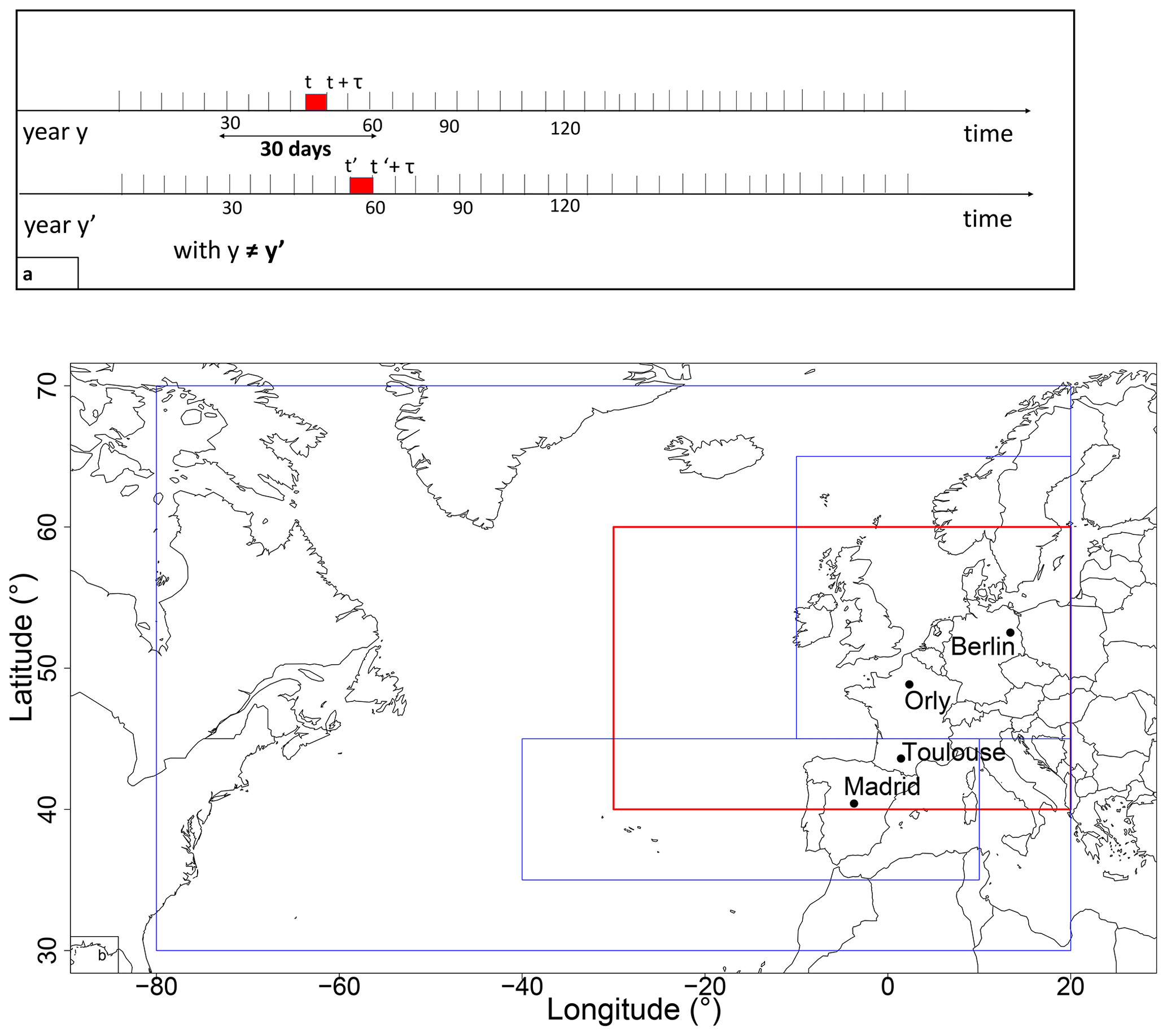
Figure 1 Parameters of the analog computation. (a) For each day t in year y, we chose an analog day t^′ with a similar sequence of τ consecutive day Z500 patterns. t₀ is selected within 30 calendar days of t and in a year $y^{\prime }\ne y$. (b) Domains of computation of analogs. We computed analogs over different domains, each one including a part of the Atlantic and focusing on a part of western Europe, in order to test the sensitivity of our model to different geographic areas. The optimizing area was [30^∘ W–20^∘ E; 40–60^∘ N], indicated by the red rectangle.

3.2 Configuration of stochastic weather generator

We use a stochastic weather generator (SWG) based on a random sampling of the circulation analogs. The operation of the SWG and its design are detailed by Yiou and Déandréis (2019). The aim is to generate random trajectories from the previously computed analogs. Therefore, to generate a trajectory, we proceed as follows: for a given day t₀ in year y₀, we generate a set of N=100 simulations until a time t₀+T, with a lead time $T\in \mathit{\{}\mathrm{5},\mathrm{10},\mathrm{20}\mathit{\}}$ d. We start at day t₀ and randomly select an analog (out of K analogs) of day t₀+1. The random selection of analogs of the day t₀+1 is performed with weights that are proportional to the calendar difference between t₀ and analog dates, to ensure that time goes forward. We also exclude analog dates with years that are equal to y₀. This rule is important for the next iterations. We then replace t₀ by the selected analog of t₀+1 and repeat the operation T times. Excluding analogs in year y₀ from the selection ensures that we do not use information from the T days that follow t₀. Hence, we obtain a hindcast trajectory between t₀ and t₀+T.

The procedure presented above is repeated N=100 times to simulate N=100 trajectories from t₀ to t₀+T₀. The daily precipitation of each trajectory is time averaged between t₀ and t₀+T. Hence, we obtain an ensemble of N=100 forecasts of the average precipitation for day t₀ and lead time T.

Then t₀ is shifted by Δt≥1 d, and the ensemble simulation procedure is repeated. This provides a set of ensemble forecasts with analogs.

We made a hindcast exercise, where the forecasts of precipitations based on analogs of atmospheric circulation (Z500), are started every Δt≈ $T/\mathrm{2}$ d between 1 January 1948 and 31 December 2019. This yields a stochastic ensemble hindcast of precipitation and atmospheric circulation (Z500). In this paper, therefore, we analyze the properties of an ensemble forecast of mean precipitation between t₀ and t₀+T. To evaluate our forecasts, the predictions made with the SWG are compared with the persistence and climatological forecasts. The persistence forecast consists of using the average value between t₀−T and t₀ for a given year. The climatological forecast takes the climatological mean between t₀ and t₀+T. The two “reference” forecasts are randomized by adding a small Gaussian noise, whose standard deviation is estimated by bootstrapping over T long intervals. We thus generate sets of persistence forecasts and climatological forecasts that are consistent with the observations (Yiou and Déandréis, 2019).

The simulations of this stochastic model will be called “SWG forecasts”, as opposed to ECMWF forecasts.

3.3 Forecast verification

Forecast verification is the process of determining the statistical quality of forecasts. A wide variety of ensemble forecast verification procedures exists (Jolliffe and Stephenson, 2012; Wilks, 1995)​​​​​​​. They involve measures of the relationship between a set of forecasts and corresponding observations. To assess the quality of precipitation forecasts, we compute indicators such as the correlation and continuous rank probability skill score (CRPSS) for each lead time T, for different seasons and months.

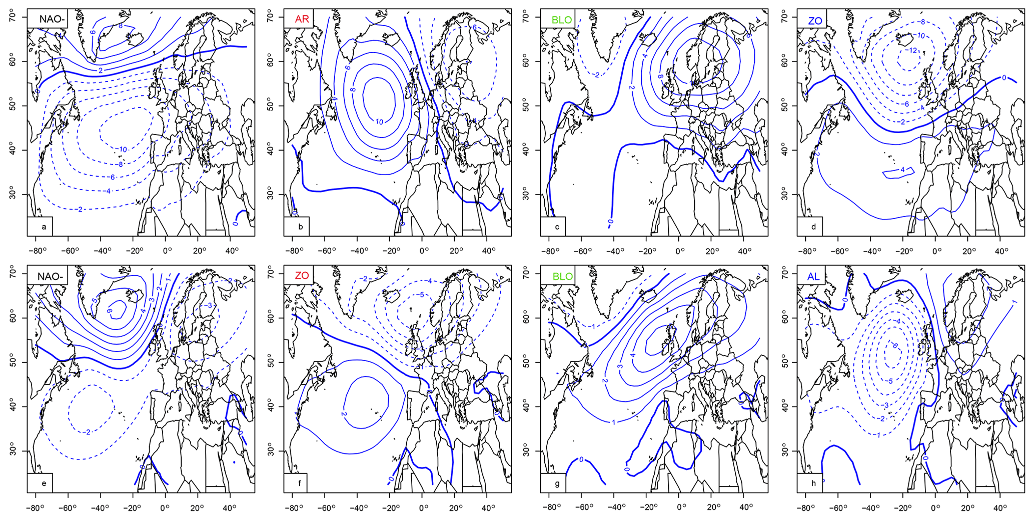
Figure 2 Weather regimes over Europe from SLP fields. Upper panels (a)–(d) contain winter (December–January–February: DJF) regimes: negative phase of the North Atlantic oscillation (NAO−), Atlantic Ridge (AR), Scandinavian blocking (BLO), and Zonal regime (ZO). Lower panels (e)–(h) contain summer (June–July–August: JJA) weather regimes: negative phase of the North Atlantic oscillation (NAO−), Zonal (ZO), Scandinavian blocking (BLO) and Atlantic low (AL). The isolines show seasonal anomalies with respect to a DJF and JJA, in hPa with 2 hPa increments.

The temporal rank correlation (referred to as correlation skill) is calculated between the precipitation observations and the median of 100 simulations. This simple diagnostic is often used to assess forecast skills of indices (Scaife et al., 2014).

The continuous ranked probability score (CRPS) is widely used for probabilistic forecast verification (Ferro, 2007). It is sensitive to the distance between forecast and observation probability distributions.

If the ensemble forecast x yields a probability distribution P(x) for a value x_a, the CRPS measures how the probability distribution of x compares with x_a (Hersbach, 2000).

The CRPS is computed as

$$\begin{array}{}\text{(2)}& \mathrm{CRPS}(P,x_a)=\underset{-\mathrm{\infty }}{\overset{+\mathrm{\infty }}{\int }}{\left(P\left(x\right)-\mathcal{H}(x-x_a)\right)}^{\mathrm{2}}\mathrm{d}x,\end{array}$$

where x_a is the observation and ℋ is the Heaviside function of the occurrence of x_a (ℋ(y)=1 if y≥0, and ℋ(y)=0 otherwise). The decomposition and properties of the CRPS have been investigated by Ferro (2007), Hersbach (2000), and Zamo and Naveau (2018). A perfect forecast would have a CRPS equal to 0, but the CRPS value obviously depends on the units of the variable to forecast, so quantifying what is a “good” forecast requires a normalization. It is hence difficult to compare CRPS values for temperature and precipitation, within the same ensemble forecast. This issue is also acute for non-Gaussian variables with heavy tails (Zamo and Naveau, 2018) so that the interpretation of a given CRPS value might not be informative.

One way of circumventing this difficulty is to compare CRPS values to reference forecasts, such as persistence or climatology. The continuous rank probability skill score (CRPSS) is a normalization of Eq. (2) with respect to such a reference.

The CRPSS is hence computed by

$$\begin{array}{}\text{(3)}& \mathrm{CRPSS}=\mathrm{1}-{\displaystyle \frac{\stackrel{\mathrm{‾}}{\mathrm{CRPS}}}{\stackrel{\mathrm{‾}}{{\mathrm{CRPS}}_{\mathrm{ref}}}}},\end{array}$$

where $\stackrel{\mathrm{‾}}{\mathrm{CRPS}}$ is the time average of the CRPS of the SWG forecast and $\stackrel{\mathrm{‾}}{{\mathrm{CRPS}}_{\mathrm{ref}}}$ is the time average of the CRPS of the reference (either climatology or persistence). The CRPSS is interpreted as a fraction of improvement over a reference forecast.

The values of the CRPSS vary between −∞ and 1. The forecast is considered to be an improvement over the reference when the CRPSS value is positive. Values of CRPSS equal to 0 indicate no improvement over the reference. Values inferior to 0 mean that the forecast is worse than the reference.

We use the CRPSS values to determine the maximum lead time T for which the SWG forecast is better than references. Then the SWG assessments will use the CRPS and directly compare the probability distributions of precipitation ensemble forecasts.

3.4 Dependence of forecast on weather regimes

We investigated the role of North Atlantic weather patterns on the forecast quality by attributing CRPS values of the SWG precipitation simulations to weather regimes. Weather regimes are defined as large-scale quasi-stationary atmospheric states. They are characterized by their recurrence, persistence, and stationarity (Michelangeli et al., 1995). They help in describing the features of the atmospheric circulation. Surface variables like temperature and precipitation are largely correlated with weather regimes (van der Wiel et al., 2019).

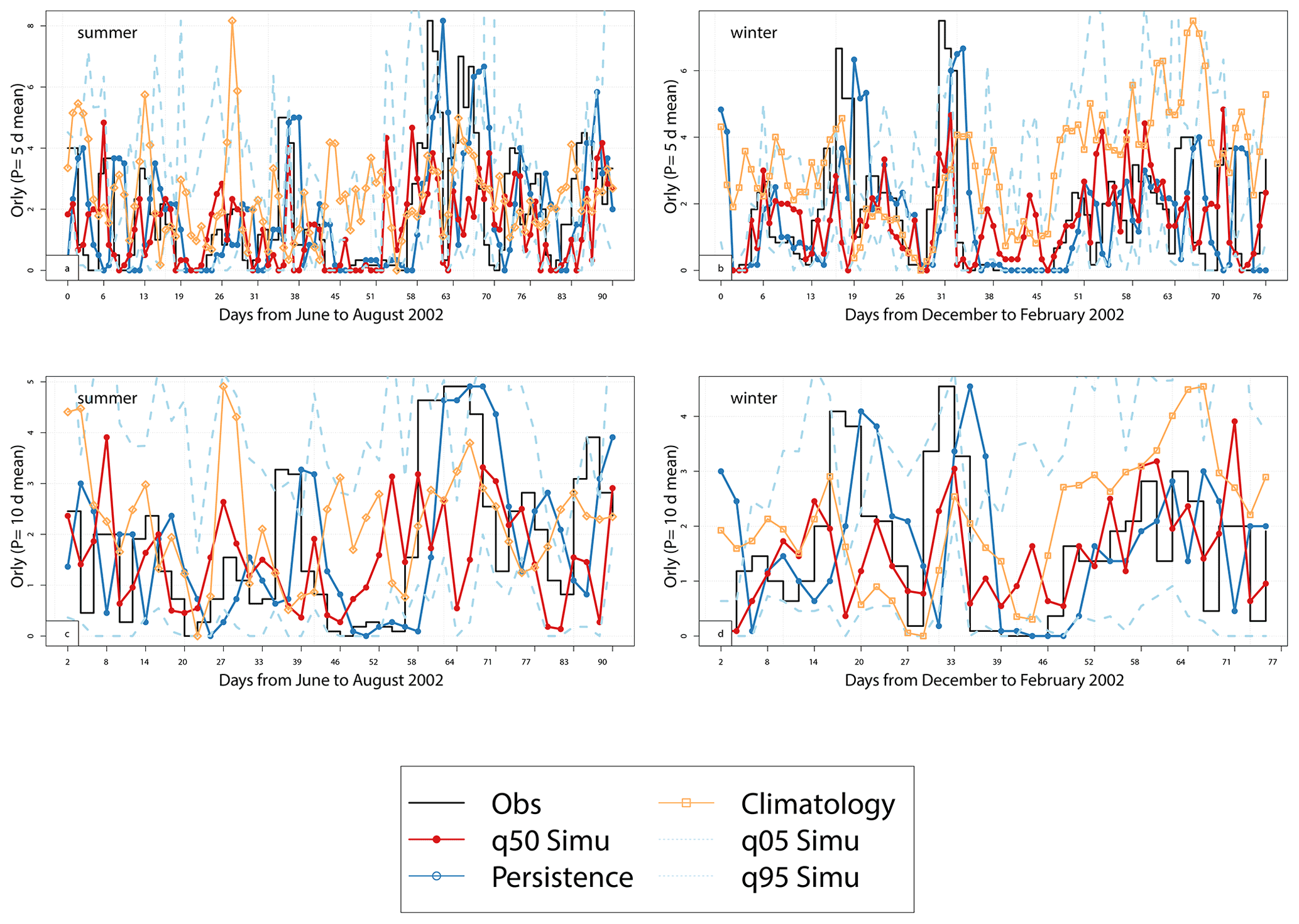
Figure 3 Time series of analog ensemble forecasts for 2002, for lead times of 5 d (a, b) and 10 d (c, d)​​​​​​​ for summer (June to August) (a) and (c) and winter (December to February) (b) and (d) for Orly. The median of 100 simulations is represented by the red line. The black line represents observation values. Dashed lines represent the 5th and 95th quantiles. The blue line represents the persistence forecasts and the orange line represents the climatology forecasts. The y-axis represents the average precipitation over T=5, 10 d.

The North Atlantic weather regimes were computed with the procedure of Yiou et al. (2008), with the NCEP reanalysis. The first 10 principal components of SLP (large region in Fig. 1b) were classified with a k-means algorithm onto four classes over a reference period between 1970 and 2010. The procedure was repeated 100 times with random k-means initialization. Then we classified the resulting 100×4 k-means weather regimes in order to determine the most probable classification. This heuristic procedure increases the robustness of the obtained weather regimes. Figure 2 shows four weather regimes for each season (winter and summer) that are coherent with the literature (Cassou et al., 2011; Ghil et al., 2008; Kimoto, 2001; Michelangeli et al., 1995).

The winter weather regimes are the negative phase of the North Atlantic oscillation (NAO−), Atlantic Ridge (AR), Scandinavian blocking (BLO), and Zonal (ZO). The summer weather regimes are the negative phase of the NAO (NAO−), Zonal (ZO), Scandinavian blocking (BLO), and Atlantic low (AL). The regimes are not the same in both seasons due to the seasonality of the large-scale atmospheric circulation.

For each day (in winter and summer) between 1948 and 2019, we classified the SLP by minimizing the root mean square to four reference (1970–2010) weather regimes.

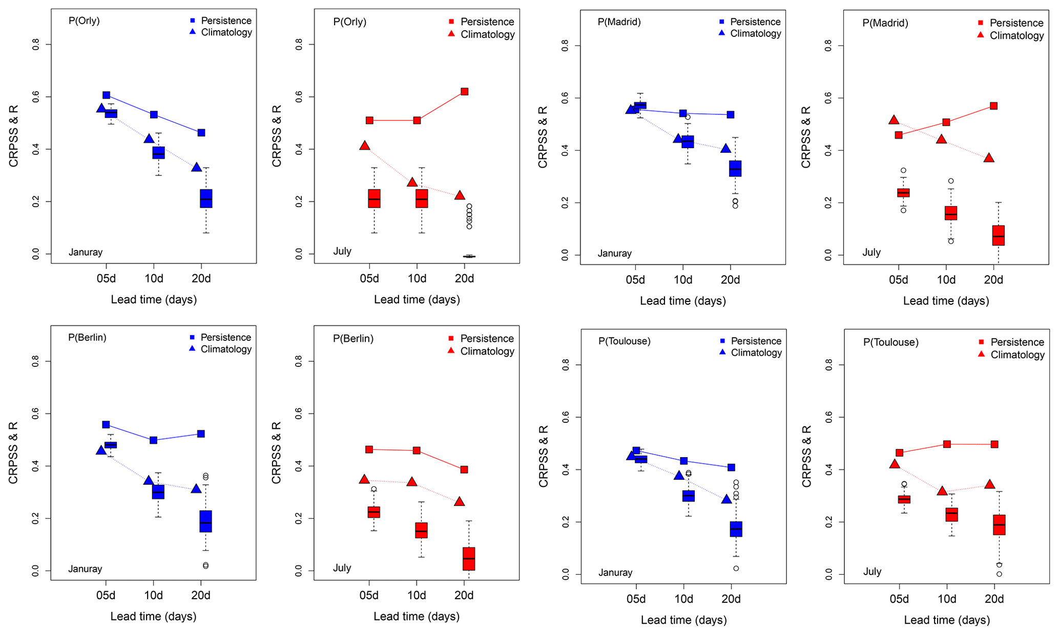
Figure 4 Skill scores for the precipitation of Orly, Madrid, Berlin, and Toulouse for lead times of 5, 10, 20 d for January (blue) and July (red) for analogs computed from reanalyses of NCEP. Squares indicate CRPSS where the persistence is the baseline, triangles indicate CRPSS where the climatology is the reference, and boxplots indicate the probability distribution of correlation between observation and the median of 100 simulations for all days. The boxplot upper whisker is: $min\left\{\mathrm{1.5}(q_{\mathrm{75}}-q_{\mathrm{50}})+q_{\mathrm{50}},max\left(\mathrm{CRPSS}\right)\right\}$. The boxplot lower whisker is: $max\left\{q_{\mathrm{50}}-\mathrm{1.5}(q_{\mathrm{75}}-q_{\mathrm{50}}),min\left(\mathrm{CRPSS}\right)\right\}$.

For each day t (within a given season), we considered the analog dates of all N=100 simulations between t and t+T and the corresponding classification into weather regimes. Then we determined the most frequent weather regime of the N member ensemble forecast between t and t+T. We hence obtained time series on the most likely weather pattern that dominates in the ensemble forecast between t and t+T.

We evaluated the influence of the dominating weather regimes on the SWG forecast quality by plotting the probability distribution of CRPS values conditioned on the weather regimes. This is done separately for “good” forecasts (low CRPS values) and “poor” forecasts (high CRPS values).

We identified two classes of predictability from CRPS values:

• Low predictability is related to high values of CRPS that exceed the 75th quantile.

• High predictability is linked to low values of CRPS, below the 25th quantile.

Then we associated the dominating weather regimes computed above with classes of high or low predictability. This procedure helps in identifying atmospheric patterns that could lead to low or high predictability with the SWG model.

4 Stochastic weather generator parameter optimization

We started by verifying the relationship between Z500 over the Euro-Atlantic region and the precipitation in the four studied areas to ensure that Z500 analogs would be reasonable predictors of precipitation. We show the maps of the temporal rank correlation between the daily average of Z500 and the precipitation in Appendix B1. We found a significant negative correlation between Z500 and the precipitation with p values ≤0.05.

Then we empirically adjusted the parameters of the SWG simulations to optimize the forecast scores. The first parameter is the geographic area. We computed sample trajectories of the SWG for the four domains outlined in Fig. 1b. We used different domains in order to find an optimal region that allows verifying the relationship between precipitation and Z500 for the four studied areas. Each domain included a part of the Atlantic and a part of western Europe. We chose the widest domain with the coordinates 80^∘ W–20^∘ E and 30–70^∘ N in order to catch the variability in the whole Euro-Atlantic region; however, this large domain gave the poorest skill scores for precipitation forecasting for the studied areas as shown in Table 1. Then we focused on two smaller domains (outlined in blue in Fig. 1b): one centered over northern Europe and the other centered over southern Europe. We found better forecast skills for specific locations. The same level of performance was found for the domain (outlined in red in Fig. 1b) with coordinates 30^∘ W–20^∘ E and 40–60^∘ N. Therefore, we kept this domain for the subsequent analyses, because it allows optimizing the correlations between Z500 and precipitation for the four studied areas and the time of computation of analogs at the same time. We compared the skill scores over the geographic domain with the coordinates [80^∘ W–20^∘ E; 30–70^∘ N] and [30^∘ W–20^∘ E; 40–60^∘ N]. We determined that the SWG simulations showed a better skill for the geographic domain (outlined in red in Fig. 1b) and the skill scores remained the highest ones as represented in Table 1.

Table 1 Correlation between observations and the median of 100 simulations for the winter (DJF) for the different studied domains represented in Fig. 1b, with the coordinates [80^∘ W–20^∘ E; 30–70^∘ N] for the largest one (blue) and [30^∘ W–20^∘ E; 40^∘–60^∘ N] for the red rectangle for a lead time of 5 d.

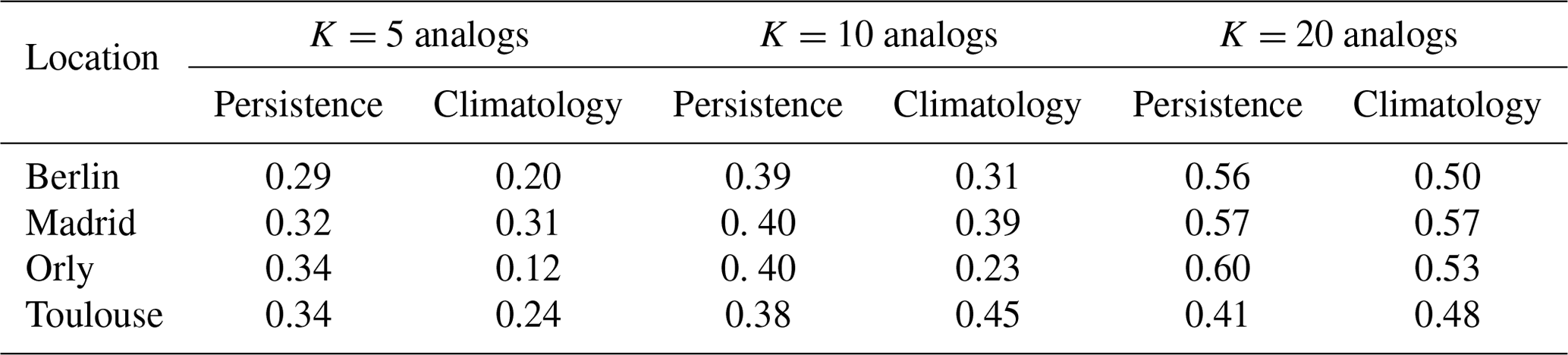
The second parameter is the number K of the best analogs that we use to simulate the precipitation. Our choice was based on numerical experiments. We performed different SWG simulations where we varied the number of analogs (K=5, 10, 20). We noticed an improvement in the skill scores by increasing the number of analogs as shown in Table 2. Therefore, we considered K=20 analogs to ensure that we had enough analog dates for the simulations. It appears that the Euclidean distance of analogs grows rather slowly after K=20. Our choice was also supported by a theoretical study by (Platzer et al., 2021) who showed that, for complex systems, the use of a large number of analogs (K>30 analogs) does not change the prediction properties with analogs. Thus, we kept K=20 best analogs for the rest of the analyses.

Table 2 CRPSS versus persistence and climatology for SWG simulations with 5, 10, and 20 analogs for the [30^∘ W–20^∘ E; 40–60^∘ N] domain and for a lead time of 5 d.

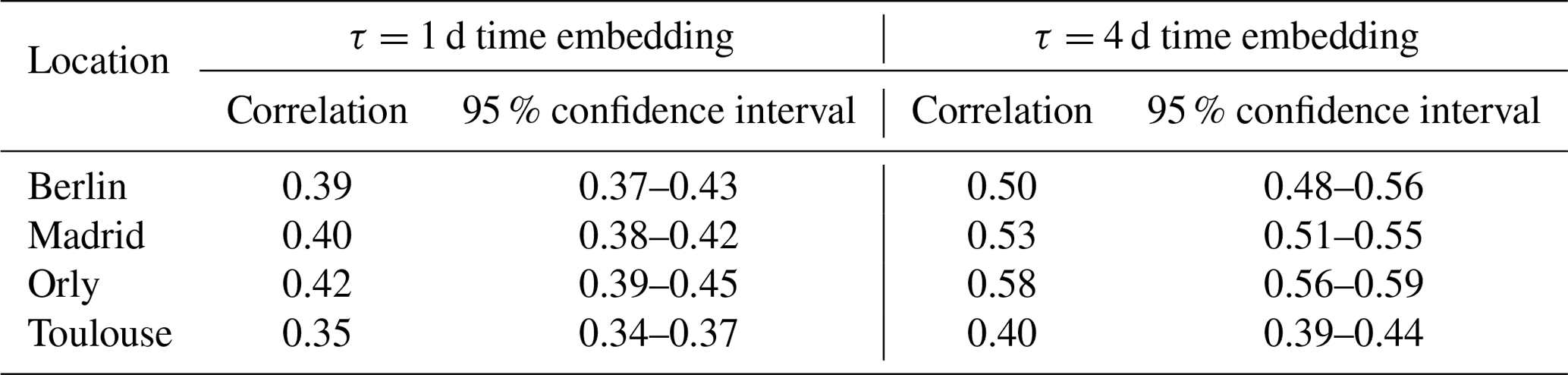
We quantified the dependence of the forecast on the time embedding for the analogs τ by calculating the analogs based on different embedding values from τ=1– 4 d. We found that an embedding of 4 d helped to better catch the persistence and improve the skill scores for the forecast compared with 1 d, as shown in Table 3. Therefore, we kept the forecast based on a 4 d embedding. This choice was based on the numerical experiments performed for the studied locations. This is also supported by the study of Yiou et al. (2013), where the analog computation with time embedding was argued to improve the temporal smoothness of simulations. With such an embedding, forecasts for lead times of T=5 d yield at least two time increments.

Table 3 Correlation between observations and the median of 100 simulations for the winter (DJF) based on analogs computed with an embedding of 1 and 4 d for the geographic domain with the coordinates [30^∘ W–20^∘ E; 40–60^∘ N] for a lead time of 5 d.

For comparison purposes, SWG simulations are obtained using analogs computed from reanalyses on the NCEP and ERA5 reanalyses. By comparing their skill scores, we found that CRPSS and correlations between observations and simulations are positive in both cases, and show positive improvement compared with persistence and climatology forecasts. The CRPSS and correlation for simulations with analogs of NCEP are almost identical to those with ERA5, as shown in Table 4. Therefore, we focused on SWG simulations with analogs from the NCEP reanalysis in the sequel as both NCEP and ERA5 (1950–2019) have the same skill, as shown in Table 4, and because NCEP is easier to handle due to its lower horizontal resolution. The computations were made using observations of precipitation from the ECAD (Klein Tank et al., 2002) and E-Obs (Haylock et al., 2008) databases. We found the same results because the ECAD and E-Obs are highly correlated (by the construction of E-Obs).

Table 4 Comparison between the values of the CRPSS of SWG computed using different reanalysis datasets for NCEP and ERA5 from 1979 to 2019 for a lead time of T=5 d for winter (DJF).

In summary, we made the forecast of the precipitation using K=20 analogs computed from Z500 over the [30^∘ W–20^∘ E; 40–60^∘ N] domain (red rectangle in Fig. 1b). To compute analogs, we used NCEP reanalyses and an embedding of τ=4 d. The computations were based on ECAD observations (Klein Tank et al., 2002).

5 Results

5.1 Sample forecast

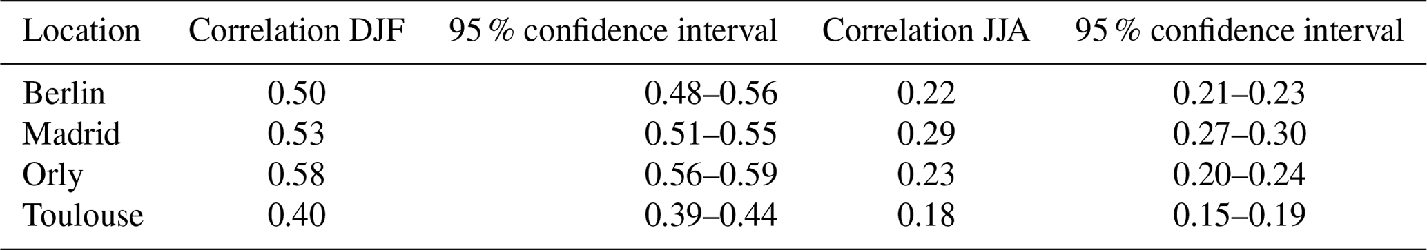
As an example, we illustrate the behavior of the trajectories in Orly for the summer and winter of 2002. Figure 3 shows the observed and simulated values of precipitation for lead times of 5 and 10 d for summer (June–July–August: JJA) and winter (December–January–February: DJF), for Orly precipitation data. We observe significantly positive correlations between observed values and the median of the forecasts for the four data sets as represented in Table 5. The correlation is generally smaller in the summer than in the winter. The correlation skill is low for some extreme values of precipitation. For a lead time of 10 d, SWG simulation still shows a capacity to predict precipitation, in particular for winter with a correlation equal to 0.23 (Orly), 0.30 (Berlin), 0.43 (Madrid), and 0.31 (Toulouse).

Table 5 Correlation between observations and the median of 100 simulations for both seasons, winter (DJF) and summer (JJA), for a lead time of 5 d.

We observe that the 5th and 95th quantiles of the simulations include the different values of observations. This heuristically confirms the good skill of SWG to forecast precipitation from Z500 for various seasons (winter and summer) in several locations for T=5 and T=10 d lead times.

The difference in the forecast correlation skills between the four studied locations may be related to the variation of the local climate from one region to another. The studied areas are in different climate types according to the Köppen–Geiger climate classification (Peel et al., 2007). From the southwestern side of Europe, Madrid is in the arid zone of the classification (Peel et al., 2007), which indicates that convective rains are less frequent, and the origin of precipitation might be the result of humidity coming from the Atlantic. Conversely, Berlin is located in a cold zone characterized by warm summer and the absence of a dry season (Peel et al., 2007); the precipitation could be the result of both, convective rains and Atlantic humidity.

In this paper, we decided (for simplicity) to use the same analogs to forecast precipitation for those four stations as discussed in Sect. 4. A refinement of the analog regions would be necessary when focusing on Madrid vs. Berlin.

5.2 Forecast probability skill

The CRPSS and correlation skill scores are computed for the four studied stations (Berlin, Madrid, Orly, and Toulouse), as shown in Fig. 4 and for lead times from 5 to 20 d.

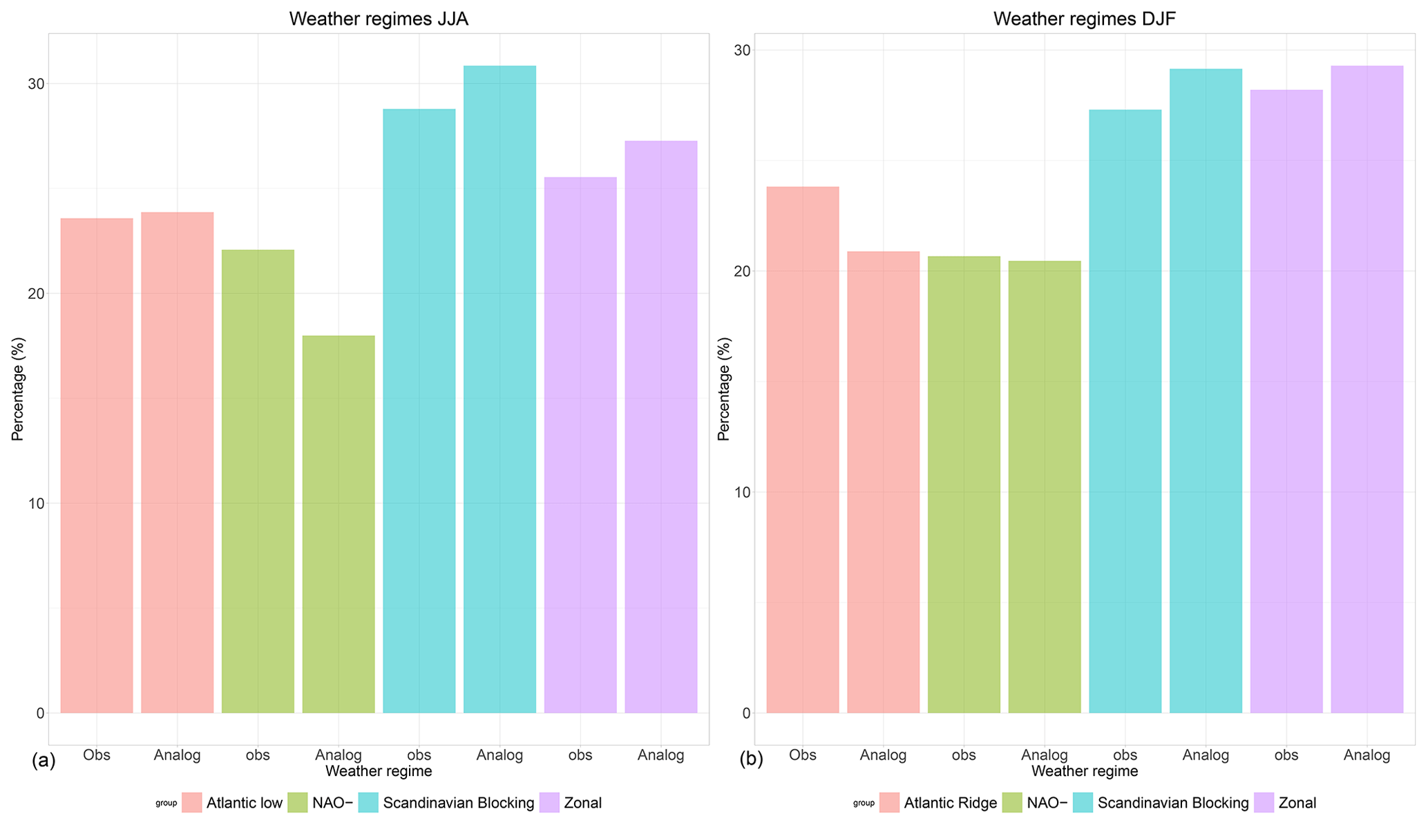
Figure 5 Percentage of each weather regime for observations dates (Obs) and the most frequent weather regime from SWG simulations between t₀ and $t_{\mathrm{0}}+T=\mathrm{5}$ d (Analog) over the period from 1948 to 2019 for summer (JJA: a) and winter (DJF: b). The percentage of weather regime is the same in Obs and Analog.

In this paper, we chose to present the results for summer and winter to highlight the capacity of the SWG to forecast the precipitation in extreme seasons. We focus on January and July in order to show the skill of the SWG in predicting precipitation in different conditions.

The CRPSS against the persistence and climatology references show positive values for lead times of up to 20 d (Fig. 4). The values of CRPSS against the persistence reference (represented by squares) decrease with lead times in winter for the different studied areas, showing high values over 5 d. However, for summer, we notice that the values of CRPSS against persistence increase with lead time, with high values over 20 d except for Berlin. This indicates that the SWG forecast is still better than the persistence forecast (the average of the CRPS of SWG is smaller than the average of the CRPS of the persistence) for lead times of 20 d in the summer. This could be explained by the fact that summer precipitation in Orly (51 % of the time, on average) comes in clusters contrary to precipitation in Berlin. Indeed, we computed the seasonal frequency of precipitation (defined as the number of days when precipitation exceeds 0.5 mm d⁻¹). We found that for Berlin, precipitation exceeding 0.5 mm d⁻¹ is more frequent than in the other stations (close to 50 % of the time for both seasons).

This means that a persistence forecast for Orly is likely to be skillful, even for longer lead times, especially in the summer. Therefore, the trends in CRPSS values for different lead times are probably due to the intrinsic time persistence of local precipitation.

The CRPSS against the climatology reference (triangles in Fig. 4) shows lower values compared with the CRPSS against persistence reference, although they are positive for all lead times and for both seasons. However, we notice that for a short lead time the SWG is better than the climatology.

The correlation skill is positive for both seasons but higher in winter (January) than in summer (July). For a lead time of 5 d, the correlation is equal to 0.59 for Madrid, 0.50 for Berlin, and 0.40 for Toulouse. For a lead time of 10 d, it is equal to 0.42 for Madrid, 0.30 for Berlin, and 0.41 for Toulouse.

The SWG was tested by Yiou and Déandréis (2019) to forecast temperature in western Europe. Comparing the performance of the SWG to forecast those different meteorologic variables, we noticed that the model shows good performance to forecast the temperature in the winter; also the best performance of the model is at a lead time of 5 d. We find that the skill scores (CRPSS and correlation) decrease with lead times. The forecast skill of the SWG shows variability from one location to another. However, the model was able to forecast temperature until 40 d in Berlin, Orly, and Toulouse with positive skill scores.

From a visual inspection of the CRPSS and correlations, we chose to focus on lead times of T=5 d, for which the correlation exceeds 0.5 in the winter. It is rather low in the summer, due to convective events leading to a high precipitation variability (from no rain to very high values). Correlation scores become barely significant for lead times of 20 d, so that, like temperature, the SWG should not be used beyond that horizon.

5.3 Relation between weather regimes and CRPS

We investigated the role of North Atlantic weather patterns defined in Sect. 3.4 (Fig. 2) on the forecast skill of the SWG precipitation simulations.

We started by comparing the frequencies of the weather regimes from the observations and the most frequent weather regime found in SWG simulations for a given lead time T=5 d. We found that the percentages are very similar (Fig. 5). This means that the weather regimes of the simulated trajectories do not yield major biases for the summer or winter seasons.

Then we looked at the relation between weather regimes and CRPS values by using the most frequent weather regime within T days and the two classes of quantiles of the CRPS that related to good quality of forecast (attributed to low values of CRPS ≤q₂₅) and poor quality of forecast (attributed to high values of CRPS ≥q₇₅). This relation is represented in Fig. 6 for Orly and for the rest of the studied stations in Fig. A1. We found a small influence of specific weather regimes on the CRPS distribution for summer.

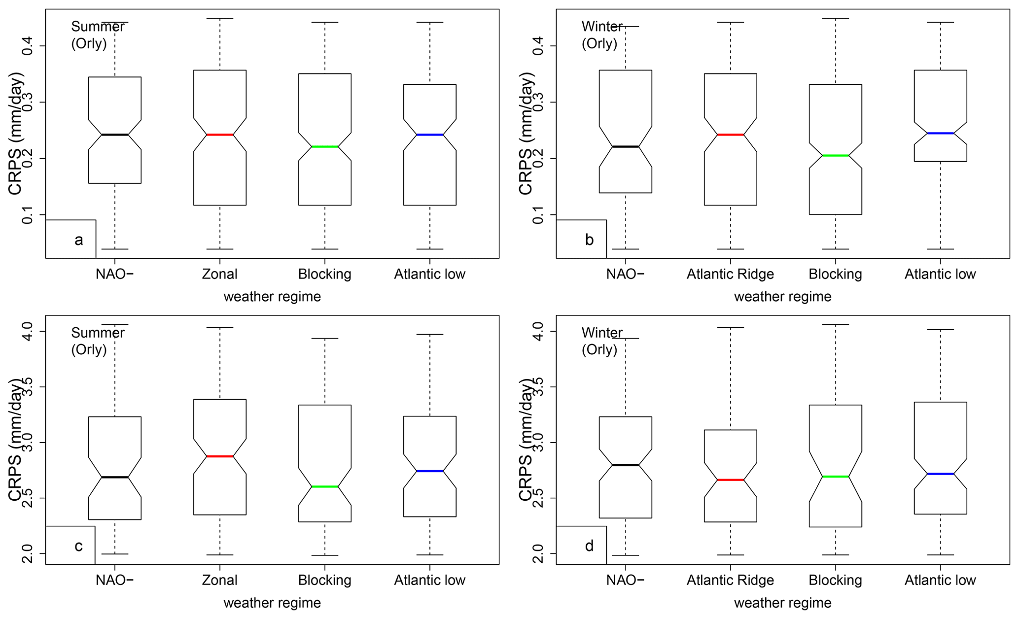
Figure 6 Relation between CRPS and weather regimes for Orly, for SWG forecasts with lead time T=5 d. Panels (a) and (b) show CRPS value distribution conditioned on four weather regimes, when CRPS is lower than q₂₅. Panels (c) and (d) show that CRPS is higher than q₇₅. The boxplots indicate the median (q₅₀) of the distribution (thick bar). The 25th (q₂₅) and 75th (q₇₅) quartiles (lower and upper segments of each boxplot). The boxplot upper whisker is $min\left\{\mathrm{1.5}(q_{\mathrm{75}}-q_{\mathrm{50}})+q_{\mathrm{50}},max\left(\mathrm{CRPS}\right)\right\}$. The boxplot lower whisker is $max\left\{q_{\mathrm{50}}-\mathrm{1.5}(q_{\mathrm{75}}-q_{\mathrm{50}}),min\left(\mathrm{CRPS}\right)\right\}$.

The weather regime signal for “good” forecasts depends on the season and the considered station. When the forecast has a low CRPS value (for Orly), we find that the Scandinavian blocking regime slightly dominates (green bar in Fig. 6a, b). This is also the case for Berlin (in winter) and Toulouse (Fig. A1b, j). The low CRPS values in Madrid are obtained for the Atlantic Ridge regime (Fig. A1f).

The weather regime signal for “poor” forecasts also yields a dependence on the season and station. Higher CRPS values are obtained with the Zonal regime in the summer for Orly (red line in Fig. 6c) and Toulouse. The Atlantic Ridge regime favors high CRPS values (i.e., poor forecasts) for Madrid in winter Fig. A1h. The Scandinavian blocking favors high CRPS values for Berlin in winter and summer (green line in Fig. A1c and d). The different impacts of the weather regimes on the studied areas are related to the position of the high- and low-pressure regions of each weather regime in the studied areas.

This relation between predictability (or the CRPS distribution) and weather regimes, albeit weak, is consistent with previous work of Faranda et al. (2017). Similar relations were found between weather regimes over Europe and the temperature in a recent study by Ardilouze et al. (2021). We found that the sensitivity of the forecast to weather regime is larger for low values of CRPS and in winter. The sensitivity of forecast skill to weather regimes is rather small on average, even for small lead times (T=5 d).

5.4 Comparison with ECMWF forecast

We first compared the CRPSS of SWG forecasts for winter and summer with the CRPSS of ECMWF forecasts.

The CRPSS of the ECMWF forecast is computed for different lead times going from 1 to 10 d for precipitation (Haiden et al., 2018) over the region 12.5^∘ W–42.5^∘ E; 35.0–75.0^∘ N (ECMWF, 2020). It uses the climatology as a reference (Haiden et al., 2018). The values of CRPSS for Europe for 2020 decrease in accordance with lead times (Haiden et al., 2018). The CRPSS of ECMWF is about 0.16 in summer (JJA) and 0.25 in winter (DJF) for a lead time of T=5 d (ECMWF, 2020). The CRPSS of SWG simulations for a lead time of T=5 d is shown in Table 4. The values suggest that the predictive skill of SWG is qualitatively promising for short lead times, compared with ECMWF forecasts. However, we have to mention that the values of CRPSS for ECMWF are computed over all of Europe for both seasons (Haiden et al., 2018), while with the SWG we are doing a forecast for local stations.

We made a quantitative comparison between the two forecasts for the different lead times. We computed the CRPS for the ECMWF forecast. Then we used the Kolmogorov–Smirnov (KS) test (von Storch and Zwiers, 2001, chap. 1) to compare the probability distributions of the CRPS of SWG and ECMWF forecasts. The null hypothesis supposes that the CRPS of ECMWF and SWG forecasts have the same distribution. The null hypothesis of the KS test was rejected; this means that the two time series do not have the same distribution, with a p value =0.11. A similar result was found by Ardilouze et al. (2021), where they compared the efficiency between ECMWF and CNRM forecasts.

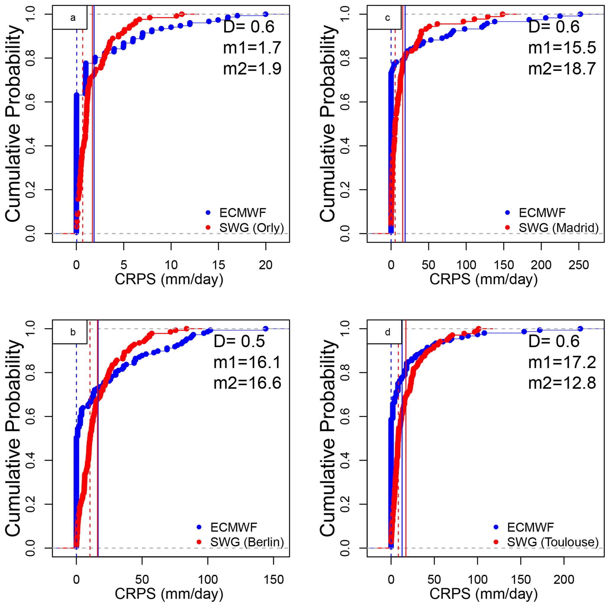
Figure 7 Empirical cumulative distribution function of the CRPS of ECMWF (blue) and SWG (red) forecasts for 5 d, for Orly (a), Berlin (b), Madrid (c), and Toulouse (d). D is the maximum distance between both ECDFs (value of Kolmogorov–Smirnov test). m1 is the value of the time average of CRPS of SWG and m2 is the value of the time average of CRPS of ECMWF. The dashed vertical lines represent the median of CRPS of ECMWF (blue) and SWG (red).

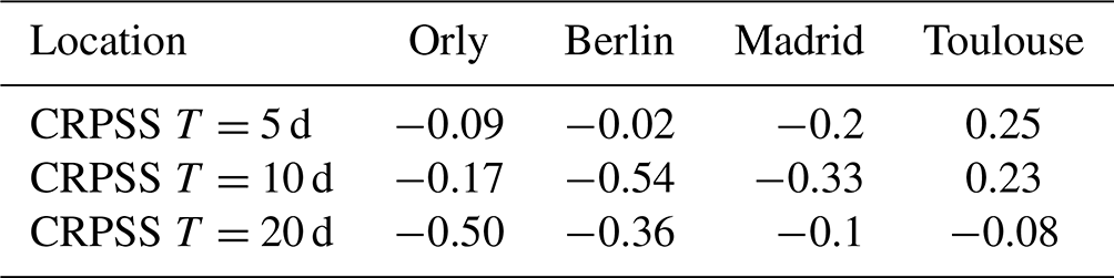
Table 6 CRPSS of ECMWF forecasts using as a reference the CRPS of SWG, for lead times of T=5, 10, and 20 d. The forecasts show that the SWG has a positive improvement compared with the ECMWF forecast as the CRPSS scores are above zero, except for that of Toulouse.

We found that 80 %, 39 %, 50 %, and 40 % of the CRPS of SWG forecast are equal to zero for, respectively, Orly, Berlin, Madrid, and Toulouse, for a lead time of T=5 d Fig. 7, which shows the capacity of the SWG to simulate rain events well. One notable difference between SWG and ECMWF forecasts is that although the proportion of CRPS values close to zero is higher for ECMWF, the CRPS for the worst forecasts is much higher than those of SWG. Indeed, we noticed that the time average of CRPS of ECMWF (vertical blue lines) and SWG (red vertical lines) for T=5 d are close, with higher values for ECMWF (Fig. 7). However, the median CRPS of ECMWF is smaller compared with the SWG (dashed vertical lines in Fig. 7). Finally, we computed the CRPSS for ECMWF forecasts taking as a reference the CRPS of SWG (Table 6). We hence computed the CRPSS of ECMWF forecast by normalizing the CRPS by the CRPS of the SWG forecast in Eq. (C1).

This new ECMWF CRPSS evaluates the added value of the ECMWF forecast over the SWG forecast. We found that the ECMWF forecast has no improvement over the SWG forecast for the different lead times because the CRPSS values are negative. At T=5 d, we noticed that the improvement is negligible for Orly and Berlin, while it is much better for Madrid. However, for Toulouse, the ECMWF forecast still has better skills for lead times of T=5 and 10 d. For a lead time of T=10 d, the improvement of the SWG forecast over the ECMWF is significant, particularly for Berlin and Madrid. There is a major improvement for a lead time of T=20 d for Orly and Berlin.

This confirms the relatively good skill of the SWG to forecast precipitation, compared with ECMWF. This could be explained by the difference in the average of the CRPS of the two forecasts. Indeed, as we mentioned before, the ECMWF forecast yields the best skill scores for small values of precipitations (<2 mm d⁻¹). We further illustrate those comparisons in Fig. C1 and Table C1.

6 Conclusions

In this work, we have shown the performance of a stochastic weather generator (SWG) to simulate precipitation over different locations in western Europe and for various time scales from 5 to 20 d. The input of our model was analogs of geopotential heights at 500 hPa (Z500). The choice of such input was made in order to evaluate the impact of large-scale circulation on local weather variables. The SWG showed a good skill in predicting precipitation for a lead time of 5 and 10 d from analogs of Z500.

This study of precipitation forecast complements the work of Yiou and Déandréis (2019) initially made to forecast temperature and the NAO index. We explored the sensitivity of the SWG model on analogs computed from different geographic areas and from different reanalyses (ERA5 and NCEP). We found that both NCEP and ERA5 reanalyses perform well for simulations.

We evaluated the relation between the quality of the forecast and weather regimes over Europe. We found that low and high predictability were related to specific weather regimes. This dependence is more significant in winter than in summer. We found that good predictability is mainly related to blocking.

A comparison with the ECMWF forecast system over western Europe confirmed quantitatively and qualitatively the skill forecast of the SWG , for lead times of T≤10 d. Of course, the SWG model cannot replace a numerical weather prediction, as the SWG parameters (e.g., region of analogs) need to be tuned to local variables and rely on the existence of a fairly large database to compute analogs. Here we used the same domain of circulation analogs for stations from Madrid to Berlin. Obviously, this region should be optimized for each individual station. Therefore, the main utility of the SWG forecast system is to make local ensemble simulations, where its performances can challenge a numerical weather prediction if the parameters are well tuned.

This paper hence confirms the proof of concept to generate ensembles of (local) precipitation forecasts from analogs of circulation. The SWG ensemble forecast performance relies on the relation between precipitation and the synoptic atmospheric circulation, which is verified for western Europe. Transposing this SWG to other regions of the globe requires observations covering several decades. Numerical weather models obviously do not yield this constraint.

Appendix A: CRPS and weather regimes

To avoid a tedious redundancy we deferred the figures of evaluation of the forecast quality by weather regimes to this appendix section.

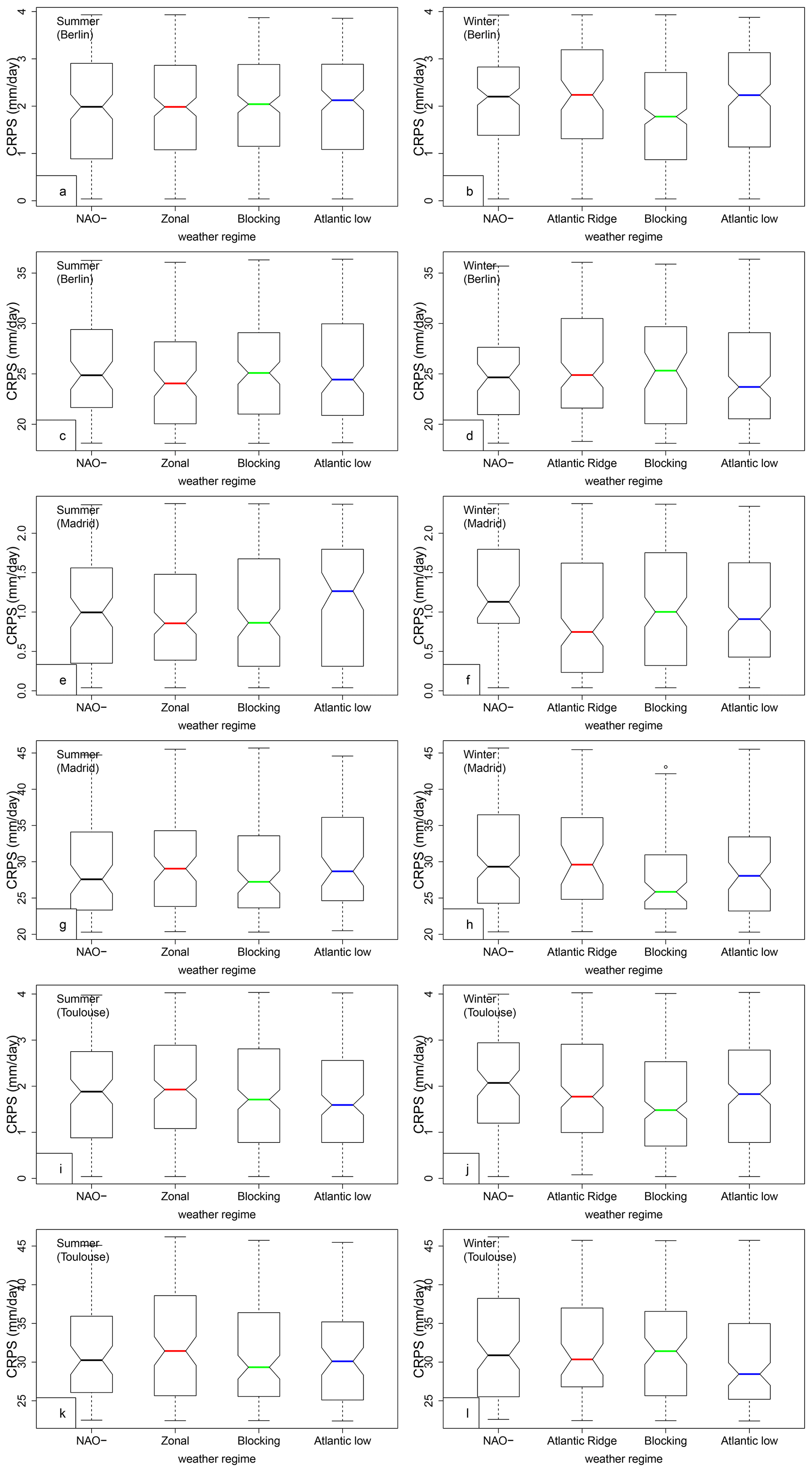
Figure A1 Relation between CRPS and weather regimes for Berlin (a–d), Madrid (e–h), and Toulouse (i–l), for SWG forecasts with lead time T=5 d. Panels (a), (b), (e), (f), (i), and (j) correspond to CRPS value distribution conditioned on four weather regimes, when CRPS is lower than q₂₅. Panels (c), (d), (g), (h), (k), and (l) correspond to a higher CRPS value (CRPS≥q₇₅). The boxplots indicate the median (q₅₀) of the distribution (thick bar).

Appendix B: Relation between Z500 and precipitation

In order to justify the use of the Z500 as a driver of precipitation, we computed the rank spatial correlation between the daily average of Z500 over the Euro-Atlantic region and the precipitation in each studied station (Berlin, Madrid, Orly, and Toulouse). We did the analysis for different seasons (DJF and JJA). We found a maximum correlation amplitude of −0.5 for Madrid and Orly, and a correlation of −0.4 and −0.3, respectively, for Toulouse and Berlin. The correlation is significant as we have a p value <0.05 for the different grid points. This indicates the relation between Z500 patterns and precipitation, in particular in western Europe, and that a decrease in Z500 is linked with precipitation.

Figure B1 Maps of correlation between Z500 and precipitation in Berlin, Madrid, Orly, and Toulouse for the period from 1948 to 2019 over the Euro-Atlantic region. The rectangles represent the domains of computation of analogs. The optimized area [30^∘ W–20^∘ E; 40–60^∘ N] is highlighted by the red rectangle.

Appendix C: CRPSS of ECMWF vs. SWG

We explain further the comparison that we made between the ECMWF forecast and the SWG forecast. As mentioned we found that the SWG has improved compared with the ECMWF forecast. This is related to the difference in the time average of the CRPS of the two forecasts. We computed the CRPSS as follows:

$$\begin{array}{}\text{(C1)}& \mathrm{CRPSS}=\mathrm{1}-{\displaystyle \frac{\stackrel{\mathrm{‾}}{{\mathrm{CRPS}}_{\mathrm{ECMWF}}}}{\stackrel{\mathrm{‾}}{{\mathrm{CRPS}}_{\mathrm{SWG}}}}},\end{array}$$

where $\stackrel{\mathrm{‾}}{{\mathrm{CRPS}}_{\mathrm{ECMWF}}}$ is the time average of the CRPS of the ECMWF forecast and $\stackrel{\mathrm{‾}}{{\mathrm{CRPS}}_{\mathrm{SWG}}}$ is the time average of the CRPS of the SWG.

Table C1 Average and median values of CRPS, average CRPSS (in bold) of the ECMWF and SWG forecasts for lead times of T=5, 10, and 20 d. The table shows that the CRPS of the SWG forecast has a smaller average than the CRPS of the ECMWF forecast, which explains the values of CRPSS for the different studied areas and the positive improvement of the SWG compared with the ECMWF.​​​​​​​

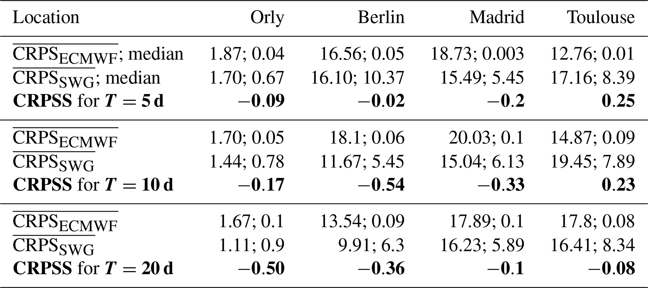
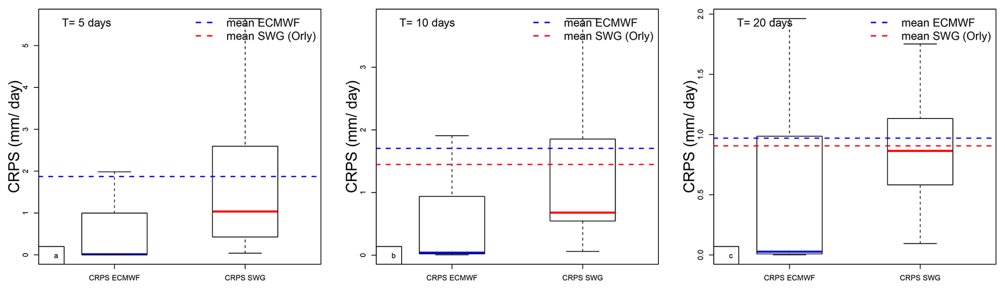
Figure C1 Boxplots of CRPS of ECMWF and CRPS of SWG for Orly, with lead time T=5, 10, and 20 d. The boxplots indicate the median (q₅₀​​​​​​​) of the distribution (thick blue bar for ECMWF and red for SWG). The 25th (q₂₅​​​​​​​) and 75th (q₇₅) quartiles are, respectively, the lower and upper segments of each boxes. The upper whisker is $min\mathit{\{}max(X),q_{\mathrm{50}}+\mathrm{1.5}(q_{\mathrm{75}}\mathrm{-}{q}_{\mathrm{25}}\left)\mathit{\right\}}$​​​​​​​. The average CRPS of the ECMWF and SWG forecasts are indicated with dashed horizontal lines. Note that the distribution is asymmetric as the median and the average are unequal. The average CRPS for the SWG forecast is lower than the average CRPS for the ECMWF forecast. The outliers that are above the upper whiskers are not shown.