Snow Multidata Mapping and Modeling (S3M) 5.1: a distributed cryospheric model with dry and wet snow, data assimilation, glacier mass balance, and debris-driven melt

By shifting winter precipitation into summer freshet, the cryosphere supports life across the world. The sensitivity of this mechanism to climate and the role played by the cryosphere in the Earth's energy budget have motivated the development of a broad spectrum of predictive models. Such models represent seasonal snow and glaciers with various complexities and generally are not integrated with hydrologic models describing the fate of meltwater through the hydrologic budget. We present Snow Multidata Mapping and Modeling (S3M) v5.1, a spatially explicit and hydrology-oriented cryospheric model that simulates seasonal snow and glacier evolution through time and that can be natively coupled with distributed hydrologic models. Model physics include precipitation-phase partitioning, snow and glacier mass balances, snow rheology and hydraulics, a hybrid temperature-index and radiation-driven melt parametrization, and a data-assimilation protocol. Comparatively novel aspects of S3M are an explicit representation of the spatial patterns of snow liquid-water content, the implementation of the Δh parametrization for distributed ice-thickness change, and the inclusion of a distributed debris-driven melt factor. Focusing on its operational implementation in the northwestern Italian Alps, we show that S3M provides robust predictions of the snow and glacier mass balances at multiple scales, thus delivering the necessary information to support real-world hydrologic operations. S3M is well suited for both operational flood forecasting and basic research, including future scenarios of the fate of the cryosphere and water supply in a warming climate. The model is open source, and the paper comprises a user manual as well as resources to prepare input data and set up computational environments and libraries.

1 Introduction

The cryosphere is a decisive driver of the Earth system (Barry, 2011; Beniston et al., 2018). Besides altering surface albedo and so concurring with the regulation of global temperature (Flanner et al., 2011), snow and glaciers accumulate winter precipitation and release it during the warm, spring and summer seasons, when demand by societies and ecosystem services is comparatively high (Barnett et al., 2005). This shift in water supply supports water, food, and energy security across climates (Viviroli et al., 2007), with key societal implications (Sturm et al., 2017). For example, snow represents up to 80 % of annual water supply in the semi-arid, largely summer-dry western US (Bales et al., 2006; Serreze et al., 1999; Skiles et al., 2018), while 1.4+ billion people in Asia rely on discharge from high-mountain, cryosphere-dominated regions (Immerzeel et al., 2010). The Andean cryosphere acts as a significant freshwater resource for semi-arid regions of South America (Masiokas et al., 2020), with an estimated contribution of up to 27 % to dry-season water supply in La Paz, Bolivia (Soruco et al., 2015).

Seasonality between winter accumulation and summer melt (Barnett et al., 2005), compounded by equally complex but more short-term processes such as rain on snow (Rössler et al., 2014), challenges decision makers like water-resource or hydropower managers, who need early and diverse information about snow and glacier-ice amount, distribution, and melt timing to make accurate decisions on water use, allocation, and storage (Georgakakos et al., 2004; Anghileri et al., 2016; Avanzi et al., 2018). This need has catalyzed the development of a variety of models to predict snowmelt- and ice-melt-driven discharge (DeWalle and Rango, 2011) to the extent that cryosphere modeling is a dominating topic of both basic and applied contemporary geosciences (Dozier et al., 2016). Applications for cryosphere models are not limited to water-supply and flood forecasting but include avalanche hazard forecasting (Bartelt and Lehning, 2002; Vionnet et al., 2012), land-surface and weather modeling (Dutra et al., 2010; Wang et al., 2017), and snowmaking (Hanzer et al., 2020). The projected rise in future temperature and aridity (IPCC, 2021) further prioritizes robust predictions of cryospheric water resources, because shrinking glaciers and decreasing snow accumulation may endanger water supply and its predictability (Harrison and Bales, 2016) – especially during droughts (Huning and AghaKouchak, 2020).

Cryospheric models intersect hydrology with thermodynamics and rheology and as such present a bewildering variety in process representation. Regarding seasonal snow, options range from detailed, physics-based micro-scale models to intermediate-complexity, energy balance models and simple one-layer, temperature-index models. Some examples of such models include SNOWPACK (Bartelt and Lehning, 2002), Crocus (Vionnet et al., 2012), SMAP (Niwano et al., 2012), UEB (Tarboton and Luce, 1996), SNOBAL (Marks et al., 1998), GEOtop (Zanotti et al., 2004; Rigon et al., 2006; Endrizzi et al., 2014), the Factorial Snowpack Model (Essery, 2015), SRM (Martinec, 1975), or HyS (De Michele et al., 2013; Avanzi et al., 2015), among many others. From a glacier standpoint, the most recurring distinction resides around glacier movement being captured through complex ice-flow approaches (Jouvet and Huss, 2019), glacier-specific parametrizations of changes in thickness (Huss et al., 2010), an equilibrium relationship between glacier area and long-term climate (Schaefli et al., 2007), or non-dynamic mass balance (Bongio et al., 2016). Parametrizing melt beneath supraglacial debris is another frequent aspect of modeling discretion (Fyffe et al., 2014).

While detail in process representation may appear to be the prime driver of model selection, in hydrologic practice this choice also depends on other four pragmatic factors, which make hydrology-oriented cryospheric models essentially different from those oriented to, e.g., avalanche hazard forecasting. First, streamflow generation in cold regions involves not only snow and glacier ice, but also precipitation–topography interactions (Blanchet et al., 2009; Mott et al., 2014; Cui et al., 2020), vegetation–water feedback mechanisms (Zheng et al., 2016; Avanzi et al., 2020), and soil-water storage (Bales et al., 2011). Thus, snow and ice hydrology is inherently spatially distributed and multi-scale (Dozier et al., 2016), with the focus being arguably more on distributed than on point predictions (Blöschl, 1999). Second, high-elevation cryospheric regions remain largely ungauged (Rasmussen et al., 2012; Avanzi et al., 2021), meaning that the necessary input data to run complex models are often missing or sparse at best. This condition has favored parsimonious models (Bartolini et al., 2011) and data-assimilation schemes to remedy model deficiencies with independently observed data (Andreadis and Lettenmaier, 2006; Piazzi et al., 2018). Coupled with data sparsity is the third factor, that is, the evidence that simplified and complex models often yield comparable predictive accuracy for bulk processes relevant to the seasonal freshet, such as snow and ice water equivalent (Huss et al., 2010; Avanzi et al., 2016; Magnusson et al., 2015). This explains why hydrology-oriented cryospheric models tend to have low complexity when it comes to internal layering and micro-scale properties. Fourth, processes relevant to cryosphere water resources span horizons from a few hours (such as rain-on-snow events; see Würzer et al., 2017) to decades (such as glacier dynamics; see Huss et al., 2010), implying that models used for real-world forecasting must be efficient enough to provide landscape-scale predictions in a timely manner (say a few hours; see Pagano et al., 2014). Ultimately, these four factors trace back to empiricism rather than reductionism being the dominant (and perhaps most successful) paradigm in hydrology (Savenije, 2009), owing to unresolved issues related to upscaling mechanistic laws to the landscape and measuring the complete heterogeneity of hydrologic processes (Blöschl and Sivapalan, 1995; Beven, 2006).

Here, we present Snow Multidata Mapping and Modeling (S3M) v5.1, a snow and glacier model developed by the CIMA Research Foundation (https://www.cimafoundation.org/, last access: 23 June 2022). Specific aspects of interest in S3M are (1) a spatially explicit prediction of both dry- and wet-snow spatial patterns as well as bulk snowpack liquid water content (θ_W, in vol %), an increasingly decisive variable for snowmelt and avalanche hazard forecasting (Techel and Pielmeier, 2011; Mitterer et al., 2013; Wever et al., 2014; Avanzi et al., 2015; Wever et al., 2016), (2) the combination of both snow and glacier mass dynamics in a coherent modeling framework, including the so-called Δh parametrization by Huss et al. (2010) and melt beneath supraglacial debris, and (3) provisions for assimilating various decision-relevant variables like snow water equivalent (SWE), snow depth, and satellite-based snow-cover area. S3M v5.1 is the last generation of a model originally proposed by Boni et al. (2010) but significantly developed thereafter (henceforth, simply S3M).

The paper is organized as follows: Sect. 2 focuses on model description, including both snow and glaciers. Section 3 presents an example of results for an inner Alpine valley in northwestern Italy where various versions of this model have been operational since the 2000s (Aosta Valley). Finally, Sect. 4 discusses model applicability and future developments. The Supplement includes a user manual discussing run preparation, execution, and post-processing.

2 Model description

The main modeling philosophy behind S3M is to provide a ready-to-use tool for applications over large areas and when a short turnaround is needed. Thus, S3M complies with the four pragmatic factors of operational, hydrology-oriented cryospheric models outlined in the Introduction, including being spatially distributed, parsimonious for both input-data requirements and complexity, and computationally efficient enough to be deployed in operational, real-time flood-forecasting chains (Laiolo et al., 2014). These chains generally ingest an ensemble of weather predictions, may include parameter and/or state perturbation, assimilate remote-sensed and in situ measurements, and must provide predictions for a variety of closure sections across the landscape in a matter of hours (Pagano et al., 2014). As such, they tend to be much more conceptually and computationally simple than research-oriented Earth system models (Pagano et al., 2014). S3M tries to bridge the gap between these two realms by accompanying simplicity and computational efficiency with an open-source environment that allows for frequent updates and improvements.

Parsimony implies a number of trade-off choices regarding which process representation to include and at which extra cost. Current model physics include precipitation-phase partitioning, snow and glacier mass balances, a hybrid temperature-index and radiation-driven melt parametrization, snow rheology and hydraulics, and a data-assimilation protocol. Relevant drivers of snowpack and glacier evolution that are not yet included comprise internal snowpack energetics and the full energy balance, longwave losses, turbulent heat fluxes, sublimation, and canopy–snow interactions. While the recent literature has shown that the added value of complex, physics-based snow models over more parsimonious alternatives for variables that are relevant to hydrology may sometimes be elusive (Rutter et al., 2009; Magnusson et al., 2015; Zaramella et al., 2019; Girons Lopez et al., 2020; Günther et al., 2019), designing more holistic and physics-based operational models remains a key to achieving the most accurate representation of snow temporal dynamics and spatial patterns, especially at fine resolutions (see, for example, the results in Lafaysse et al., 2017; Vionnet et al., 2021). Strategies to include these processes in future releases of S3M are discussed in Sect. 4.

S3M is a raster-based model, with the same set of equations being solved for each cell and no lateral mass or energy transfer besides glacier change in thickness. All input, state, and output variables are distributed, meaning they are passed to the model as rasters with fixed resolution in geographic degrees (see the Supplement). Spatial resolution can be set by the user (we will consider a ∼240 m resolution in our example of application in Sect. 3). All equations are ordinary differential equations with no need for iterative computations, so they are solved for all pixels in the simulation domain using a forward Euler method, as this method provides comparatively high numerical stability and minimizes computational time. The time step of the model is flexible, but it is generally set to 1 h.

2.1 Definitions

We define snow and glacier ice as a mixture of three constituents: ice, liquid water, and air. Following De Michele et al. (2013) and Avanzi et al. (2015), the control volume of unitary area (h_TOT) for each pixel of the simulation domain is defined as

$$\begin{array}{}\text{(1)}& h_{\mathrm{TOT}}=h_{\mathrm{G}}+h_{\mathrm{S}}={\displaystyle \frac{V_{\mathrm{tot}}}{A}},\end{array}$$

where h_G is glacier thickness (m), h_S is the height of snow (often referred to as snow depth, m), V_tot is the control volume (m³), and A is the area of the pixel (m²). $h_{\mathrm{G}}=V_{\mathrm{G}}/A$ and $h_{\mathrm{S}}=V_{\mathrm{S}}/A$, where V_G and V_S are the total volume of glacier and snow within the pixel under study. We define M_S and M_G as the mass of seasonal snow and glacier ice for each pixel, respectively (kg). As for seasonal snow, this mass is $M_{\mathrm{S}}=M_{\mathrm{D}}+M_{\mathrm{W}}$, with M_D and M_W the mass of the dry (snow grains) and wet (interstitial liquid water) constituents, respectively. The mass of air is assumed to be negligible compared to M_D and M_W (De Michele et al., 2013).

Snow is a foam of ice (Kirchner et al., 2001), meaning that the dry constituent occupies a porous skeleton of height h_D (m, volume V_D) and porosity $n=h_{\mathrm{P}}/h_{\mathrm{D}}$ (–), where h_P is the height of pores in the mixture (m, volume V_P). Thus, we define the density of the solid skeleton ρ_D (kg m⁻³) as

$$\begin{array}{}\text{(2)}& {\mathit{\rho }}_{\mathrm{D}}={\displaystyle \frac{M_{\mathrm{D}}}{V_{\mathrm{D}}}}={\displaystyle \frac{{\mathit{\rho }}_{\mathrm{i}}(V_{\mathrm{D}}-V_{\mathrm{P}})}{V_{\mathrm{D}}}}={\mathit{\rho }}_{\mathrm{i}}(\mathrm{1}-n),\end{array}$$

where ρ_i=917 kg m⁻³ is ice density. The density of the wet constituent is equal to that of liquid water: ${\mathit{\rho }}_{\mathrm{W}}=M_{\mathrm{W}}/V_{\mathrm{W}}=\mathrm{1000}$ kg m⁻³ (V_W is the volume of liquid water in the mixture, height h_W). The density of glacier ice is assumed equal to ρ_i, with no progressive compression and/or air expulsion from cavities (Cuffey and Paterson, 2010).

During most of the snow season, the dry and wet constituents of the snowpack are both contained in h_D, the prevalent volume. However, an oversaturation condition takes place during the last instants of the snow season due to phase change (De Michele et al., 2013). Despite being a limited, virtually unmeasurable scenario, including this oversaturation condition is important from a numerical-stability standpoint. Thus, the total control volume of snow h_S (that is, snow depth) is hereby defined as

$$\begin{array}{}\text{(3)}& h_{\mathrm{S}}=h_{\mathrm{D}}+\langle h_{\mathrm{W}}-n{h}_{\mathrm{D}}\rangle ,\end{array}$$

where 〈〉 are Macaulay brackets, which provide the argument whether this is positive and otherwise 0. In other words, h_S is equal to the height of the porous structure h_D plus – if present – the oversaturated volume 〈h_W−nh_D〉 (De Michele et al., 2013). Accordingly, the bulk snow density ρ_S (kg m⁻³) is

$$\begin{array}{}\text{(4)}& {\mathit{\rho }}_{\mathrm{S}}={\displaystyle \frac{M_{\mathrm{D}}+M_{\mathrm{W}}}{V_{\mathrm{S}}}}={\displaystyle \frac{{\mathit{\rho }}_{\mathrm{D}}{V}_{\mathrm{D}}+{\mathit{\rho }}_{\mathrm{W}}{V}_{\mathrm{W}}}{V_{\mathrm{S}}}}={\displaystyle \frac{{\mathit{\rho }}_{\mathrm{D}}{h}_{\mathrm{D}}+{\mathit{\rho }}_{\mathrm{W}}{h}_{\mathrm{W}}}{h_{\mathrm{S}}}}\end{array}$$

and snow water equivalent (m w.e.) is $\text{SWE}={\mathit{\rho }}_{\mathrm{S}}\times h_{\mathrm{S}}\times {\mathit{\rho }}_{\mathrm{W}}^{-\mathrm{1}}$. We also define the bulk volumetric liquid water content of the snowpack as

$$\begin{array}{}\text{(5)}& {\mathit{\theta }}_{\mathrm{W}}={\displaystyle \frac{V_{\mathrm{W}}}{V_{\mathrm{S}}}}={\displaystyle \frac{h_{\mathrm{W}}}{h_{\mathrm{S}}}}.\end{array}$$

Glaciers are modeled as a single-phase material, the mass of liquid water and air being negligible compared to glacier ice. Thus, the ice water equivalent for glaciers (IWE) is

$$\begin{array}{}\text{(6)}& \text{IWE}={\displaystyle \frac{{\mathit{\rho }}_{\mathrm{i}}{h}_{\mathrm{G}}}{{\mathit{\rho }}_{\mathrm{W}}}}.\end{array}$$

Figure 1 summarizes the prognostic variables and main mass fluxes of S3M. Dynamic inputs for S3M are total precipitation, air temperature, relative humidity, and incoming shortwave radiation (see the Supplement for details).

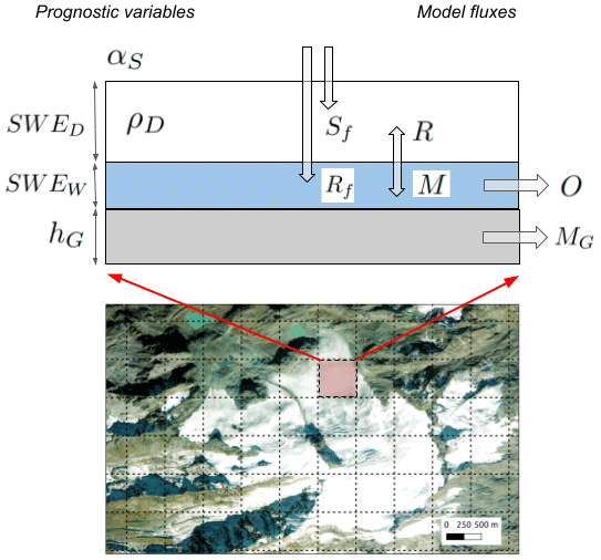
Figure 1 Prognostic variables and main mass fluxes of S3M (see Sect. 2 for details). α_S is snow albedo (–), S_f and R_f are snowfall and rainfall rate (mm Δt⁻¹), respectively, SWE_D (mm) and ρ_D (kg m⁻³) are dry snow water equivalent and dry bulk snow density, respectively, SWE_W is wet-snow water equivalent (mm), R, M, and O are snow refreezing, melt, and outflow, respectively (mm Δt⁻¹), h_G is glacier thickness (m), and M_G is ice melt (mm Δt⁻¹). Note that albedo is listed here as a prognostic variable for clarity, but the actual, underlying prognostic variable is technically snow age A_s. The background image is the Rutor glacier in northwestern Italy (ESRI Satellite theme).

2.2 Snow: mass-conservation equations

The mass-conservation equations for the dry and wet constituents of the snowpack read as follows:

$$\begin{array}{}\text{(7)}& {\displaystyle \frac{\mathrm{d}{M}_{\mathrm{D}}}{\mathrm{d}t}}=\widehat{S_{\mathrm{f}}}-\widehat{M}+\widehat{R},\text{(8)}& {\displaystyle \frac{\mathrm{d}{M}_{\mathrm{W}}}{\mathrm{d}t}}=\widehat{R_{\mathrm{f}}}+\widehat{M}-\widehat{R}-\widehat{O},\end{array}$$

where $\widehat{S_{\mathrm{f}}}$ is the snowfall mass flux, $\widehat{M}$ is the snowmelt mass flux, $\widehat{R}$ is the refreezing mass flux, $\widehat{R_{\mathrm{f}}}$ is the rainfall mass flux, and $\widehat{O}$ is the outflow mass flux (also known as snowpack runoff; see Avanzi et al., 2019). All these mass fluxes are expressed in kg Δ t⁻¹ and are denoted with a $\widehat{}$, as opposed to customary hydrologic fluxes (mm Δ t⁻¹), which will be denoted without a $\widehat{}$ in the following. Given that M_D=ρ_Dh_DA, we simplify Eq. (7) as

$$\begin{array}{}\text{(9)}& {\displaystyle \frac{\mathrm{1}}{{\mathit{\rho }}_{\mathrm{W}}A}}{\displaystyle \frac{\mathrm{d}\left({\mathit{\rho }}_{\mathrm{D}}{h}_{\mathrm{D}}A\right)}{\mathrm{d}t}}={\displaystyle \frac{\widehat{S_{\mathrm{f}}}-\widehat{M}+\widehat{R}}{{\mathit{\rho }}_{\mathrm{W}}A}}\end{array}$$

to obtain

$$\begin{array}{}\text{(10)}& {\displaystyle \frac{\mathrm{d}}{\mathrm{d}t}}\left({\displaystyle \frac{{\mathit{\rho }}_{\mathrm{D}}{h}_{\mathrm{D}}}{{\mathit{\rho }}_{\mathrm{W}}}}\right)={\displaystyle \frac{{\mathrm{dSWE}}_{\mathrm{D}}}{\mathrm{d}t}}=S_{\mathrm{f}}-M+R,\end{array}$$

where SWE_D is the dry-snow water equivalent (${\mathit{\rho }}_{\mathrm{D}}{h}_{\mathrm{D}}{\mathit{\rho }}_{\mathrm{W}}^{-\mathrm{1}}$) and S_f, M, and R are the snowfall, snowmelt, and refreezing mass fluxes in mm w.e. Δt⁻¹. Note that SWE_D and all related mass fluxes will henceforth be expressed in mm w.e., with a conversion by 1000 mm m⁻¹ being implicitly included between Eqs. (7) and (10). Likewise, we simplify Eq. (8) as

$$\begin{array}{}\text{(11)}& {\displaystyle \frac{\mathrm{1}}{{\mathit{\rho }}_{\mathrm{W}}A}}{\displaystyle \frac{\mathrm{d}\left({\mathit{\rho }}_{\mathrm{W}}{h}_{\mathrm{W}}A\right)}{\mathrm{d}t}}={\displaystyle \frac{\widehat{R_{\mathrm{f}}}+\widehat{M}-\widehat{R}-\widehat{O}}{{\mathit{\rho }}_{\mathrm{W}}A}}\end{array}$$

to obtain

$$\begin{array}{}\text{(12)}& {\displaystyle \frac{{\mathrm{dSWE}}_{\mathrm{W}}}{\mathrm{d}t}}=R_{\mathrm{f}}+M-R-O,\end{array}$$

with SWE_W being the wet-snow water equivalent and R_f and O being the rainfall and snowpack-runoff mass flux in mm w.e. (again, note that SWE_W and all related mass fluxes will henceforth be expressed in mm w.e., with a conversion by 1000 mm m⁻¹ being implicitly included between Eqs. 8 and 12).

Equations (10) and (12) are the two fundamental snow mass-conservation equations of S3M, which thus offers a spatially explicit, prognostic simulation of both the dry and wet constituents of snow (total SWE being instead a diagnostic variable: $\text{SWE}={\text{SWE}}_{\mathrm{D}}+{\text{SWE}}_{\mathrm{W}}$). This phase separation follows De Michele et al. (2013) and Avanzi et al. (2015), with two differences. First, equations in De Michele et al. (2013) and Avanzi et al. (2015) were written using h_D and h_W as the main state variables, whereas here we used SWE_D and SWE_W, which allows a more compact formulation of mass-conservation equations since no density-compaction term is necessary in Eq. (10). Second, Avanzi et al. (2015) introduced a mass-conservation equation for a third constituent, refrozen ice. Here, we directly included the refreezing term in Eqs. (10) and (12).

S3M assumes that simulated SWE as well as all other model variables and fluxes are representative of spatially averaged snowpack conditions across the simulated pixel. Whilst this assumption is coherent with current practice in many hydrologic models, it does not take advantage of scaling mechanisms with fractional snow-covered area to fully reconstruct sub-grid snow-depletion curves.

2.3 Snow: mass-flux parametrizations

Mass fluxes in Eqs. (10) and (12) requiring specific parametrizations are snowfall and rainfall (R_f and S_f), snowmelt and refreezing (M and R), and snowpack runoff (O).

2.3.1 Precipitation-phase partitioning

Snowfall and rainfall in S3M are estimated from total precipitation (P), an input for the model; precipitation-phase partitioning is based on the empirical approach described in Froidurot et al. (2014):

$$\begin{array}{}\text{(13a)}& {\displaystyle }{S}_{\mathrm{f}}=p_{\mathrm{s}}P,\text{(13b)}& {\displaystyle }{R}_{\mathrm{f}}=p_{\mathrm{r}}P,\text{(13c)}& {\displaystyle }{p}_{\mathrm{s}}=\mathrm{1}-p_{\mathrm{r}},\text{(13d)}& {\displaystyle }{p}_{\mathrm{r}}={\displaystyle \frac{\mathrm{1}}{\mathrm{1}+e^{\mathit{\alpha }+\mathit{\beta }{T}_{\mathrm{air}}+\mathit{\gamma }\text{RH}}}},\end{array}$$

where p_s and p_r are the probabilities of snowfall and rainfall, respectively, α, β, and γ are fixed parameters derived by Froidurot et al. (2014), T_air is air temperature in degrees C, and RH is relative humidity in percent. S3M assumes p_s and p_r to be equal to the actual proportions of rainfall and snowfall over total precipitation. Following Froidurot et al. (2014) and references therein, α=22, $\mathit{\beta }=-\mathrm{2.7}$, and $\mathit{\gamma }=-\mathrm{0.2}$.

Fresh snow is assumed to be dry, with density ρ_f depending on air temperature (Pomeroy and Brun, 2001):

$$\begin{array}{}\text{(14)}& {\mathit{\rho }}_{\mathrm{f}}=\mathrm{67.9}+\mathrm{51.25}{e}^{\frac{T_{\mathrm{air}}}{\mathrm{2.59}}}.\end{array}$$

2.3.2 Snowmelt and refreezing

Snowmelt (M) is computed if both concurrent T_air and mean air temperature over the previous 10 d (${\stackrel{\mathrm{‾}}{T}}_{\mathrm{10}\mathrm{d}}$) are greater than or equal to T_τ, a user-defined threshold usually assumed equal to 1 ^∘C (Pellicciotti et al., 2005); otherwise, M=0. The first condition is standard in degree-day models and accounts for snowmelt occurring during periods with a supposedly positive energy balance (meaning a net gain of energy for the snowpack). The second condition is a novel addition of S3M to the literature to keep track of cold content using a parsimonious approach (cold content being a measure of the snowpack-energy deficit to be satisfied for actual melt to start; see Jennings et al., 2018). The basic idea is that ${\stackrel{\mathrm{‾}}{T}}_{\mathrm{10}\mathrm{d}}$ evolves with a certain delay compared to T_air, so that setting an additional threshold on ${\stackrel{\mathrm{‾}}{T}}_{\mathrm{10}\mathrm{d}}$ helps avoid non-physical melt during short warm spells that come after a somewhat long cold period. Other simple approaches to estimate cold content exist, such as that based on mean-seasonal temperature by Schaefli and Huss (2011), but they are also in their early stages. Our approach is the result of intensive trial and error and specifically aims at suppressing erroneous mid-winter melt episodes that do not appear in validation data (see Sect. 3).

Snowmelt is parametrized using a hybrid physics-based and degree-day approach decoupling radiative forcing from temperature-driven melt (similarly to Pellicciotti et al., 2005):

$$\begin{array}{}\text{(15)}& M=m_{\mathrm{rad}}\left[{\displaystyle \frac{(\mathrm{1}-{\mathit{\alpha }}_{\mathrm{S}})S_{\mathrm{r}}}{{\mathit{\rho }}_{\mathrm{W}}{\mathit{\lambda }}_{\mathrm{f}}}}\right]\mathrm{\Delta }t+c_M{m}_{\mathrm{r}}\left(T_{\mathrm{air}}-T_{\mathit{\tau }}\right),\end{array}$$

where S_r is incoming shortwave radiation (an input for S3M, W m⁻²), α_S is snow broadband albedo (–), λ_f is the specific latent heat of fusion (0.334 MJ kg⁻¹), m_r is a degree-day parameter (mm ^∘C⁻¹ d⁻¹), m_rad is an a-dimensional modulating factor to convert shortwave radiation into actual melt (similar to an efficiency parameter; see below), and c_M is a timestep-adjusting parameter. While S_r is internally converted to MJ m⁻² according to the model time step (see Δt in Eq. 15), the air-temperature part of Eq. (15) is computed by first considering an equivalent day with average temperature equal to T_air, regardless of the model time step. The snowmelt part depending on air temperature is then readjusted by $c_M=\mathrm{\Delta }t/\mathrm{86}\mathrm{400}$ to pass from 1 d to the actual time step (Δt is in seconds). This workaround is due to the degree-day approach being originally conceived for daily applications (see Hock, 1999, 2003; De Michele et al., 2013, and references therein). Note that S3M internally sets S_r to 0 between 19:00 and 07:00 in order to remove spurious noise in radiation sensors (an alternative approach being the computation of sunrise and sunset time). Proper unit conversions are implicitly included in the radiation part of Eq. (15) to first pass from J m⁻² to MJ m⁻² and then from m w.e. to mm w.e.

Broadband albedo is computed once per day at midnight according to Laramie and Schaake (1972):

$$\begin{array}{}\text{(16)}& {\mathit{\alpha }}_{\mathrm{S}}=\mathrm{0.5}+\mathrm{0.45}{e}^{-{\mathit{\tau }}_{\mathit{\alpha }}{A}_{\mathrm{s}}},\end{array}$$

where τ_α is an albedo-decay coefficient equal to 0.12 d⁻¹ if average air temperature over the previous 24 h is higher than 0 ^∘C and otherwise equal to 0.05 d⁻¹. A_s is snow age (d), defined as the number of days since the last significant snowfall. S3M considers significant snowfall to be 1 d with at least 3 mm of total snowfall. Snow age A_s is updated every day at midnight: if cumulative snowfall during the previous 24 h is less than 3 mm, then snow age is increased by 1 d; if not, then snow age is reset to 0.

Similarly to other snowmelt models (Rango and Martinec, 1995), melt parameters m_r (mm ^∘C⁻¹ d⁻¹) and m_rad (–) are calibration-based, although the sensitivity of S3M to both is rather low (see results in Sect. 3). This low sensitivity is likely because explicitly separating the radiation- and temperature-driven components of melt brings these parameters closer to a fully first-principles energy balance model than standard degree-day approaches.

An explicit separation between the temperature- and radiation-driven components has been under-used in the literature. For example, the seminal work by Hock (1999) did include potential radiation but embedded it into a degree-day parameter rather than explicitly separating the radiation and temperature components. Follum et al. (2015) replaced the temperature term with a proxy from a radiation balance, which may be suitable in regions where snowmelt is mostly radiation-driven (e.g., the western US; see Bales et al., 2006) but would need some form of temperature dependency in temperate regions like the Alps.

Pellicciotti et al. (2005) are among the few examples where the radiation and the temperature component are fully decoupled, but they focused on glacier ice during summer. This isothermal condition is very efficient for shortwave radiation to convert it into actual melt. However, applying the original approach by Pellicciotti et al. (2005) to snow revealed a tendency to overestimate melt rate early in the snowmelt season, because it assumes net shortwave radiation to translate into melt regardless of the actual cold content. In subfreezing conditions, in fact, a fraction of net shortwave radiation is used to raise snow temperature, a mechanism that becomes increasingly unimportant as the season progresses and snow conditions tend towards isothermal. To mimic this transition from subfreezing to isothermal conditions, we propose a modification to the original approach by Pellicciotti et al. (2005) in the form of a novel 10 d temperature-modulated efficiency parameter m_rad that increases with ${\stackrel{\mathrm{‾}}{T}}_{\mathrm{10}\mathrm{d}}$ according to a sigmoid function (Fig. 2a):

$$\begin{array}{}\text{(17)}& \begin{array}{rl}{m}_{\mathrm{rad}}& =\mathrm{0.49338}\times \arctan (\mathrm{0.27439}\times {\stackrel{\mathrm{‾}}{T}}_{\mathrm{10}\mathrm{d}}-\mathrm{0.5988})\\ & -\mathrm{0.49338}\times {\displaystyle \frac{\mathrm{3.14}}{\mathrm{2}}}+m_{\mathrm{rad}}^{\prime }.\end{array}\end{array}$$

While parameter $m_{\mathrm{rad}}^{\prime }$ is user-defined, we note that $m_{\mathrm{rad}}^{\prime }\sim \mathrm{1.10}$ means that m_rad→1 when ${\stackrel{\mathrm{‾}}{T}}_{\mathrm{10}\mathrm{d}}>\mathrm{10}$ ^∘C. This corresponds to a 1:1 conversion of net shortwave radiation into melt when isothermal conditions like those by Pellicciotti et al. (2005) dominate. On the other hand, m_rad→0 when ${\stackrel{\mathrm{‾}}{T}}_{\mathrm{10}\mathrm{d}}\to \mathrm{0}$ ^∘C. m_rad is set to 0 if the equation above predicts a negative value. Note that this temperature-modulated efficiency parameter is a proxy of cold content, but it does not imply an explicit computation of cold content. It is an attempt to take into account thermal inertia in subfreezing conditions and how it is related to external climate, similarly to Schaefli and Huss (2011). At the present stage, no relation to snow depth or internal snow temperature is included.

S3M considers a similar relation between ${\stackrel{\mathrm{‾}}{T}}_{\mathrm{10}\mathrm{d}}$ and m_r through a sigmoid function and a user-defined tuning parameter ($m_{\mathrm{r}}^{\prime }$; see Fig. 2b):

$$\begin{array}{}\text{(18)}& \begin{array}{rl}{m}_{\mathrm{r}}& =\mathrm{0.598862}\times \arctan (\mathrm{0.27439}\times {\stackrel{\mathrm{‾}}{T}}_{\mathrm{10}\mathrm{d}}-\mathrm{0.5988})\\ & -\mathrm{0.598862}\times {\displaystyle \frac{\mathrm{3.14}}{\mathrm{2}}}+m_{\mathrm{r}}^{\prime }.\end{array}\end{array}$$

Here again, we note that $m_{\mathrm{r}}^{\prime }\sim \mathrm{1.40}$ mm C⁻¹ d⁻¹ corresponds to ∼0.05 mm C⁻¹ h⁻¹ when ${\stackrel{\mathrm{‾}}{T}}_{\mathrm{10}\mathrm{d}}>\mathrm{10}$ ^∘C, which agrees with estimates by Pellicciotti et al. (2005) in isothermal conditions on ice. While establishing a relationship between melt parameters and ${\stackrel{\mathrm{‾}}{T}}_{\mathrm{10}\mathrm{d}}$ is novel, the previous literature has already suggested a seasonal variability in the degree-day parameter that is conceptually similar to our approach (see Bongio et al., 2016, and references therein). Also, note that m_r should be much smaller than degree-day parameters listed by Hock (2003), because the latter were supposed to account for both the temperature-driven and radiation-driven components of snowmelt. Parameter m_r is set to 0 in case the equation above returned a value lower than 0.

Refreezing (R) is computed when T_air<T_τ using a simple degree-day approach as in Avanzi et al. (2015):

$$\begin{array}{}\text{(19)}& R=-c_M{m}_{\mathrm{r}}\left(T_{\mathrm{air}}-T_{\mathit{\tau }}\right).\end{array}$$

Differently from Avanzi et al. (2015) or Schaefli et al. (2014), we do not decrease m_r by a reduction factor when computing refreezing. In standard degree-day models that do not separate the temperature and radiation components of melt, that reduction factor accounts for refreezing melt rate being smaller than snowmelt rate for the same temperature difference, given the usual lack of incoming shortwave radiation during refreezing-prone periods. This reduction factor is not necessary in S3M, because the contribution of incoming shortwave radiation is explicitly accounted for in Eq. (15) and excluded in Eq. (19); in other words, m_r only accounts for turbulent and longwave-radiation factors.

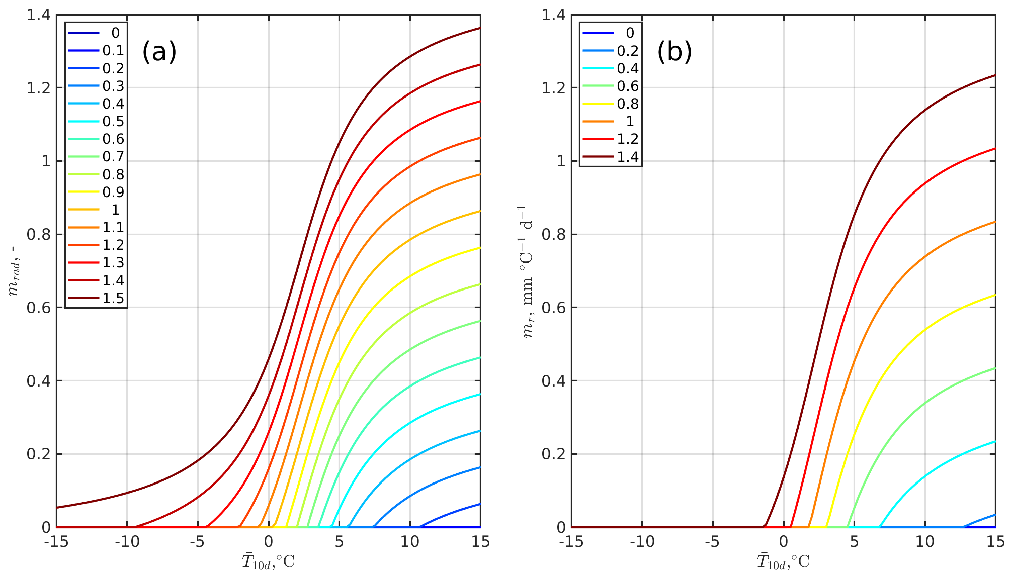
Figure 2 Values of the modulating parameter converting shortwave radiation into actual melt (m_rad, panel a) and the degree-day melt parameter (m_r, panel b) as a function of mean air temperature over the previous 10 d (${\stackrel{\mathrm{‾}}{T}}_{\mathrm{10}\mathrm{d}}$) and various values of two tuning parameters ($m_{\mathrm{rad}}^{\prime }$ and $m_{\mathrm{r}}^{\prime }$; see figure legends for values).

2.3.3 Snowpack runoff

While the term runoff in catchment hydrology generally denotes overland flow, we follow here customary nomenclature in snow hydrology and call snowpack runoff the amount of liquid water discharged by the snowpack (Wever et al., 2014). This flux is parametrized according to a matrix-flow approximation (Colbeck, 1972; Avanzi et al., 2015, 2016):

$$\begin{array}{}\text{(20)}& O=\mathit{\alpha }{\displaystyle \frac{{\mathit{\rho }}_{\mathrm{W}}g{K}_{\mathrm{W}}}{{\mathit{\mu }}_{\mathrm{W}}}},\end{array}$$

where μ_W is water dynamic viscosity, g is acceleration due to gravity, K_W is the intrinsic permeability of water in snow (m²), and α is a time- and unit-conversion parameter (equal to 1000 mm m${}^{-\mathrm{1}}\times \mathrm{\Delta }t$, with Δt in seconds). Assuming ρ_W=1000 kg m⁻³, g=9.81 m s⁻², and ${\mathit{\mu }}_{\mathrm{W}}=\mathrm{1.79}\times {\mathrm{10}}^{-\mathrm{2}}$ kg m⁻¹ s⁻¹ (DeWalle and Rango, 2011), then

$$\begin{array}{}\text{(21)}& O=\mathit{\alpha }{\mathit{\alpha }}^{\prime }{K}_{\mathrm{W}},\end{array}$$

with ${\mathit{\alpha }}^{\prime }=\mathrm{5.47}\times {\mathrm{10}}^{\mathrm{5}}$ m⁻¹ s⁻¹. We predict K_W following again Colbeck (1972):

$$\begin{array}{}\text{(22)}& K_{\mathrm{W}}=K{S}^{\star \mathrm{3}},\end{array}$$

where K is the intrinsic permeability of snow (m²) and S^⋆ is the effective saturation degree:

$$\begin{array}{}\text{(23)}& S^{\star }={\displaystyle \frac{\text{Sr}-{\text{Sr}}_i}{\mathrm{1}-{\text{Sr}}_i}}.\end{array}$$

Sr_i is the irreducible saturation degree computed based on Kelleners et al. (2009) as $\mathrm{0.02}{\mathit{\rho }}_{\mathrm{D}}{\mathit{\rho }}_{\mathrm{W}}^{-\mathrm{1}}{n}^{-\mathrm{1}}$, whereas $\text{Sr}=h_{\mathrm{W}}{n}^{-\mathrm{1}}{h}_{\mathrm{D}}^{-\mathrm{1}}$ is the saturation degree. Snowpack runoff is set to 0 if Sr<Sr_i.

Intrinsic permeability of snow is predicted based on Calonne et al. (2012):

$$\begin{array}{}\text{(24)}& K=\mathrm{3}{r}_{\mathrm{e}}^{\mathrm{2}}{e}^{-\mathrm{0.013}{\mathit{\rho }}_{\mathrm{D}}},\end{array}$$

where r_e is the equivalent sphere radius (m), a conceptual, characteristic length of snow microstructure corresponding “to the radius of a monodisperse collection of spheres having the same specific surface area (SSA) as the sample considered” (Calonne et al., 2012). Variable r_e and SSA (m² kg⁻¹) are likely the most objective metrics of snow microstructure to date (Carmagnola et al., 2014), traditional grain size being subjective and cumbersome to measure (Fierz et al., 2009). Still, SSA and r_e are insufficient to fully characterize snow structure, because grain shape also plays an important role in the two-point correlation function (Krol and Löwe, 2016). We relate r_e to SSA by definition,

$$\begin{array}{}\text{(25)}& r_{\mathrm{e}}={\displaystyle \frac{\mathrm{3}}{\text{SSA}{\mathit{\rho }}_{\mathrm{i}}}},\end{array}$$

and diagnostically estimate SSA following Domine et al. (2007):

$$\begin{array}{}\text{(26)}& {\text{SSA}}^{\prime }=-\mathrm{308.2}\ln \left({\mathit{\rho }}_{\mathrm{D}}^{\prime }\right)-\mathrm{206},\end{array}$$

with SSA^′ being SSA in cm² g⁻¹ and ${\mathit{\rho }}_{\mathrm{D}}^{\prime }$ being ρ_D in g cm⁻³. We used Eq. (26) to predict SSA because S3M does not include a prognostic simulation of snow microstructure. However, Domine et al. (2007) clearly show that density alone is a modest predictor of SSA (R²=0.43).

In order to avoid high saturation values in a shallow snowpack causing large outflow rates and non-physical negative values of SWE_W, Eq. (20) is used as long as Sr<0.5 or SWE_D>10 mm w.e. In situations with Sr≥0.5 or SWE_D<10 mm, Eq. (20) is bypassed and SWE_W is directly converted into snowpack runoff.

2.3.4 Dry-density equation

Differently from liquid water, bulk dry-snow density in S3M is not invariant with time because of three main factors: compaction, new-snow events, and refreezing:

$$\begin{array}{}\text{(27)}& {\displaystyle \frac{\mathrm{d}{\mathit{\rho }}_{\mathrm{D}}}{\mathrm{d}t}}={\displaystyle \frac{\mathrm{d}{\mathit{\rho }}_{\mathrm{D}}}{\mathrm{d}t}}{|}_{\mathrm{comp}}+{\displaystyle \frac{\mathrm{d}{\mathit{\rho }}_{\mathrm{D}}}{\mathrm{d}t}}{|}_{\mathrm{snowf}}+{\displaystyle \frac{\mathrm{d}{\mathit{\rho }}_{\mathrm{D}}}{\mathrm{d}t}}{|}_{\mathrm{ref}}.\end{array}$$

These factors do not include snow metamorphisms (Pinzer, 2009), mainly because of the scale mismatch between such processes and the one-layer approach of S3M.

Regarding compaction, we assume a linear profile for stress with depth and start from the momentum-conservation equation for a representative element at 66 % depth, which experiences an average stress:

$$\begin{array}{}\text{(28)}& {\mathit{\sigma }}_{\mathrm{v}}=\mathrm{0.66}{\mathit{\rho }}_{\mathrm{D}}g{h}_{\mathrm{D}}=\mathrm{0.66}{\text{SWE}}_{\mathrm{D}}{\mathit{\rho }}_{\mathrm{W}}g,\end{array}$$

with σ_v being vertical stress. Equation (28) is then coupled with a viscous rheological equation to obtain, via the definition of the vertical strain rate,

$$\begin{array}{}\text{(29)}& {\displaystyle \frac{\mathrm{d}{\mathit{\rho }}_{\mathrm{D}}}{\mathrm{d}t}}{|}_{\mathrm{comp}}={\mathit{\rho }}_{\mathrm{D}}{\displaystyle \frac{{\mathit{\sigma }}_{\mathrm{v}}}{\mathit{\eta }}}={\mathit{\rho }}_{\mathrm{D}}{\displaystyle \frac{\mathrm{0.66}{\text{SWE}}_{\mathrm{D}}{\mathit{\rho }}_{\mathrm{W}}g}{\mathit{\eta }}},\end{array}$$

with η being viscosity. We finally follow De Michele et al. (2013) and references therein and define viscosity as an exponential function of dry-snow density and snow temperature,

$$\begin{array}{}\text{(30)}& {\displaystyle \frac{\mathrm{d}{\mathit{\rho }}_{\mathrm{D}}}{\mathrm{d}t}}{|}_{\mathrm{comp}}=\mathrm{0.66}{c}_{\mathrm{\Delta }t}{c}_{\mathrm{1}}{\mathit{\rho }}_{\mathrm{D}}{\text{SWE}}_{\mathrm{D}}{\mathit{\rho }}_{\mathrm{W}}{e}^{\mathrm{0.08}{T}_{\mathrm{S}}-\mathrm{0.021}{\mathit{\rho }}_{\mathrm{D}}},\end{array}$$

or in a more compact form as

$$\begin{array}{}\text{(31)}& {\displaystyle \frac{\mathrm{d}{\mathit{\rho }}_{\mathrm{D}}}{\mathrm{d}t}}{|}_{\mathrm{comp}}=\mathrm{0.66}{c}_{\mathrm{\Delta }t}{c}_{\mathrm{1}}{\mathit{\rho }}_{\mathrm{D}}^{\mathrm{2}}{h}_{\mathrm{D}}{e}^{\mathrm{0.08}{T}_{\mathrm{S}}-\mathrm{0.021}{\mathit{\rho }}_{\mathrm{D}}}.\end{array}$$

T_S is snow mean temperature (^∘C), c₁=0.001 m² h⁻¹ kg⁻¹, and c_Δt is a timestep-adjusting coefficient ($\mathrm{\Delta }t\times {\mathrm{3600}}^{-\mathrm{1}}$ s⁻¹ h, with Δt in seconds).

Because S3M does not solve for the full energy balance, it also does not simulate snow-temperature profiles. The fact that snow temperature in S3M has no implication for snowmelt, compounded by the sensitivity of the settling equation to snow temperature being rather small (not reported for brevity), led us to introduce a simple parametrization here: if T_air<0 ^∘C, snow mean temperature is assumed to follow a linear profile between snow-surface temperature and ground surface (assumed equal to T_air and 0 ^∘C, respectively, following pieces of experimental evidence like Ohara and Kavvas, 2006; Filippa et al., 2014), while otherwise it is set to 0 ^∘C.

New events change bulk-snow density proportionally to snowfall depth versus existing snow depth:

$$\begin{array}{}\text{(32)}& {\mathit{\rho }}_{\mathrm{D}}(t+\mathrm{\Delta }t)={\displaystyle \frac{{\text{SWE}}_{\mathrm{D}}+S_{\mathrm{f}}}{\left(\frac{S_{\mathrm{f}}}{{\mathit{\rho }}_{\mathrm{f}}}+\frac{{\text{SWE}}_{\mathrm{D}}}{{\mathit{\rho }}_{\mathrm{D}}}\right)}}.\end{array}$$

We handle refreezing with a similar approach to new events:

$$\begin{array}{}\text{(33)}& {\mathit{\rho }}_{\mathrm{D}}(t+{\mathrm{\Delta }}_t)={\displaystyle \frac{{\text{SWE}}_{\mathrm{D}}+R}{\left(\frac{R}{{\mathit{\rho }}_{\mathrm{i}}}+\frac{{\text{SWE}}_{\mathrm{D}}}{{\mathit{\rho }}_{\mathrm{D}}}\right)}}.\end{array}$$

2.3.5 Data assimilation

The assimilation framework of S3M is a result of CIMA's operational forecasting procedures as summarized in the Flood-PROOFS suite (Laiolo et al., 2014; Avanzi et al., 2021). These procedures – external to S3M – include generating maps of snow depth and satellite-based scene classification (hence, snow-covered area – SCA) as well as processing SWE maps from third parties (e.g., from interpolation of ground manual measurements; see Avanzi et al., 2021). Given that snow depth and satellite maps are generated with a comparatively high frequency (up to daily), their assimilation in S3M is performed in correspondence to the timestamp to which they refer (these nominal timestamps must be the same for both snow-depth and satellite maps, collectively referred to as updating maps). SWE maps have various temporal frequencies (usually weekly); thus, S3M allows the user to specify a temporal window of influence, that is, a period after the official issue date of the SWE map during which the map is assumed to be valid.

Assimilation of updating maps additionally requires a kernel map and a quality map. The kernel (K) is generally an output of the geostatistics-based interpolation method employed to generate the snow-depth maps and is used to optimally combine observations and model predictions (see below). Instead, the quality map is used to automatically skip assimilation when values on this map are below a user-defined threshold. For example, the operational convention in Flood-PROOFS is to forego assimilation during days with large cloud obstruction. Thus, in Flood-PROOFS the quality map for a given day is computed as the ratio between pixels classified as snow or ground over the total number of pixels (so, in fact, this map reports the same scalar for each pixel). In this way, quality is a measure of the proportion of the satellite map that is covered by clouds. We stress, however, that this quality can be defined based on any user's need, with S3M skipping assimilation below a quality threshold even if the corresponding snow-depth map was available.

Prior to assimilation, S3M blends information from the snow depth and the SCA maps based on quality. For example, K is doubled wherever quality is 2.5 times the quality threshold and the satellite indicates ground (ID = 0). Also, snow-depth maps are set to 0 wherever quality is greater than the quality threshold and the satellite indicates ground. Finally, snow-depth maps are set to missing values wherever quality is lower than the quality threshold, modeled SWE is less than 20 mm w.e., and the satellite indicates clouds, no decision, or no data (ID = 2, 3, and −1, respectively).

SWE maps, on the other hand, use neither a quality flag nor a spatially distributed kernel, again owing to how these maps are received and handled by Flood-PROOFS. To assimilate SWE maps, K is thus assumed to be a function of time elapsed since the issue date, with no spatial variability:

$$\begin{array}{}\text{(34)}& K=W{e}^{\frac{-(t^{\prime }-t_{\mathrm{SWE}}{)}^{\mathrm{2}}}{\mathrm{0.5}{\mathit{\sigma }}^{\mathrm{2}}}},\end{array}$$

where t_SWE is the official issue time of the SWE map, t^′ is time relative to this issue date (d), and σ is equal to half of the validity days after SWE-map issue date (user-defined parameter; see the Supplement). On the same date of the issue date, $t^{\prime }=t_{\mathrm{SWE}}$, and so K=W, where W is a user-assigned maximum weight of the map to be assimilated. No quality threshold is used for SWE maps given that they are usually the result of reanalysis rather than real-time automatic processing.

Currently, S3M performs data assimilation exclusively in the form of SWE. Thus, snow-depth-map assimilation requires a preliminary step to convert snow depth into SWE via modeled bulk-snow density:

$$\begin{array}{}\text{(35)}& {\text{SWE}}_{\mathrm{obs}}={\displaystyle \frac{h_{\mathrm{S},\mathrm{obs}}\times {\mathit{\rho }}_{\mathrm{S},\mathrm{S}\mathrm{3}\mathrm{M}}}{{\mathit{\rho }}_{\mathrm{W}}}},\end{array}$$

where h_S,obs and ρ_S,S3M are observed snow depth according to the snow-depth map and simulated bulk-snow density according to S3M, respectively. This step implicitly assumes that snow density is a less relevant source of uncertainty than snow depth in estimating SWE, which is supported by snow-density temporal patterns being consistent from year to year (Mizukami and Perica, 2008).

Updating and SWE maps are assimilated into S3M using a Newtonian relaxation approach:

$$\begin{array}{}\text{(36)}& \begin{array}{rl}{\text{SWE}}_{\mathrm{S}\mathrm{3}\mathrm{M},\mathrm{post}}& ={\text{SWE}}_{\mathrm{S}\mathrm{3}\mathrm{M},\mathrm{prior}}\\ & +K\left({\text{SWE}}_{\mathrm{obs}}-{\text{SWE}}_{\mathrm{S}\mathrm{3}\mathrm{M},\mathrm{prior}}\right),\end{array}\end{array}$$

where SWE_S3M,post and SWE_S3M,prior are the a posteriori and a priori SWE. Note that Newtonian relaxation (also known as nudging) is different from direct insertion, where model estimates are directly replaced by observations; in a nudging scheme, the correction factor is proportional to the difference between observations and model outputs via a kernel weight (Boni et al., 2010; Mazzoleni et al., 2018).

After assimilating bulk SWE, a few prognostic variables of S3M are modified through factor U_SWE:

$$\begin{array}{}\text{(37)}& {\displaystyle }{U}_{\mathrm{SWE}}={\displaystyle \frac{{\text{SWE}}_{\mathrm{S}\mathrm{3}\mathrm{M},\mathrm{post}}}{{\text{SWE}}_{\mathrm{S}\mathrm{3}\mathrm{M},\mathrm{prior}}}},\text{(38)}& {\displaystyle }{\text{SWE}}_{\mathrm{D},\mathrm{S}\mathrm{3}\mathrm{M},\mathrm{post}}=U_{\mathrm{SWE}}\times {\text{SWE}}_{\mathrm{D},\mathrm{S}\mathrm{3}\mathrm{M},\mathrm{prior}},\text{(39)}& {\displaystyle }{\text{SWE}}_{\mathrm{W},\mathrm{S}\mathrm{3}\mathrm{M},\mathrm{post}}=U_{\mathrm{SWE}}\times {\text{SWE}}_{\mathrm{W},\mathrm{S}\mathrm{3}\mathrm{M},\mathrm{prior}}.\end{array}$$

This step is needed since total SWE in S3M v5.1 is only a diagnostic variable, and assimilating it does not affect model predictions unless the true prognostic variables are also modified (in this case, SWE_D and SWE_W). Factor U_SWE assumes that both the dry and wet phases are proportionally affected by data assimilation. It is also assumed that dry-snow density does not change during assimilation. Given that dry-density evolution does depend on SWE_D, this is a simplification.

S3M optionally supports assimilating only positive differences in Eq. (36), that is, only correcting modeled SWE if observations are larger than simulations. This experimental configuration helps when assimilating observed SWE aims at correcting for precipitation undercatch (Ryan et al., 2008). Such an approach is, e.g., standard in avalanche forecasting models like SNOWPACK (Lehning et al., 2002). However, assimilating only positive differences will override the SCA component of the assimilation package, because SCA assimilation in S3M is performed indirectly by setting observed snow depth to 0 in areas with observed ground.

The last step in the snow component is to perform a set of sanity checks (e.g., set to 0 all state variables where SWE →0) and to compute the snow mask, a binary map with the same size of the simulation domain reporting 1 where SWE>0.1 mm and 0 elsewhere. This mask is an important output of S3M that is sometimes used by hydrologic models to adjust process representation in areas of snow (for example, inhibiting evapotranspiration).

2.4 Glacier component

The glacier component of S3M offers three alternative modules: (1) a simple, melt-only approach with no mass balance and no snow-to-ice conversion (G1), which is usually the default choice for short-term flood-forecasting-oriented simulations; (2) a melt-only approach with mass balance but no parametrization of glacier dynamics and no snow-to-ice conversion (G2); (3) an approach with a full mass balance, a parametrization of glacier dynamics (the Δh parametrization), and snow-to-ice conversion (G3). The last two approaches are the most suitable options for long-term, climate-scenario-oriented simulations.

G1: melt-only approach

In the most basic approach (G1), glacier melt takes place on snow-free glacier pixels with a similar parametrization to that of snow (Eq. 15), with only two changes. The first is that glacier albedo α_G is constant (0.4; see Davaze et al., 2018), as opposed to snow albedo changing with snow age. The second change is that ice-melt rate (M_G) on debris-covered glaciers may be corrected compared to the theoretical melt rate on debris-free glaciers ($M_{\mathrm{G}}^{\star }$) using a multiplicative reduction factor, f_debris (Huss and Fischer, 2016):

$$\begin{array}{}\text{(40)}& M_{\mathrm{G}}=(\mathrm{1}-f_{\mathrm{debris}})M_{\mathrm{G}}^{\star }.\end{array}$$

The correction factor f_debris can be estimated with various approaches, for example, following Huss and Fischer (2016), who prescribed it based on the so-called Østrem curve. Accordingly, values of f_debris are generally smaller than 0 for very shallow debris (up to ∼5 cm) and between 0 and 1 otherwise (Nicholson and Benn, 2006). S3M expects f_debris to be a spatially distributed input parameter included in the so-called static-data suite (see the Supplement). Glacier melt is directly converted into ice runoff, with no routing (Fig. 1). Glacier pixels are defined based on a glacier mask (see the Supplement).

2.5 G2: melt-only approach with mass balance

This approach (G2) is equivalent to G1, with the only difference that glacier thickness (h_G) is dynamically updated every hour based on glacier melt. To do so, ice melt (mm w.e.) according to Eq. (15) and optionally Eq. (40) is converted to meters of ice using ice density ρ_i. The mass-conservation equation reads

$$\begin{array}{}\text{(41)}& {\displaystyle \frac{\text{dIWE}}{\mathrm{d}t}}=-M_{\mathrm{G}}.\end{array}$$

Wherever h_G→0 as a result of multi-year melt, ice melt on that pixel is not computed anymore. S3M expects h_G to be a spatially distributed input (included either in the so-called restart data or in the static data; see the Supplement). Spatially explicit datasets of h_G could come from either in situ surveys (e.g., see Colombero et al., 2019) or from estimates based on the surface mass balance and ice-flow velocities (e.g., see Rabatel et al., 2018).

2.6 G3: mass-balance approach with glacier dynamics and snow-to-ice conversion

This approach – G3, ideal for multi-year simulations – includes snow-to-ice conversion and a specific mass-redistribution approach called the Δh parametrization (Huss et al., 2010), which allows one to implicitly account for glacier-movement effects without implementing a full ice-flow model. Because the Δh parametrization is better suited for multi-year timescales rather than day-to-day thickness changes, module G3 requires the user to define the month of water-year start, so that S3M will accumulate glacier melt for each pixel throughout the water year and update h_G at the beginning of each new water year. Regardless of this accumulation procedure, ice melt is still outputted every time step, so that seasonality in runoff-generation processes is preserved. In other words, this accumulation procedure only regards changes in glacier thickness and not ice-runoff generation. This is important in case S3M was coupled with a hydrologic model.

Snow-to-ice conversion is performed by simply prescribing that, on pixels with h_G>0, any residual SWE at the end of each water year is added to h_G. Consequently, SWE as well as all snow-related bulk state variables are reset to 0. This reset is not performed in areas where SWE>0 and h_G=0 at the end of the season; in such conditions, the snowpack is maintained through the start of the new water year. This approach is less rigorous than considering firn, the intermediate step between snow and ice, even though previous work by Schaefli et al. (2005) in Switzerland showed that the use of a separate degree-day factor for firn may not significantly improve hydrologic predictions.

As for the Δh parametrization, this is presented in Huss et al. (2010) and further discussed for hydrologic models by Seibert et al. (2018), so we limit ourselves to a short overview here. This approach starts from the empirical intuition that glacier-thickness changes as a result of both the mass balance and the glacier flow have recurring patterns throughout seasons of persistently negative mass balances (Huss et al., 2010). By parametrizing these recurring patterns, the Δh parametrization allows one to simulate the effect of movement in addition to the mass balance without a complex ice-flow model. These patterns are derived by differentiating two digital surface models (Huss et al., 2010) and then fitting a glacier-specific power law like

$$\begin{array}{}\text{(42)}& \mathrm{\Delta }h=(h_{\mathrm{r}}+a{)}^{\mathit{\gamma }}+b(h_{\mathrm{r}}+a)+c,\end{array}$$

where a, γ, b, and c are calibration parameters, Δh is the change in surface elevation (normalized by the maximum decrease across all glacier pixels), and h_r is normalized glacier elevation defined as

$$\begin{array}{}\text{(43)}& h_{\mathrm{r}}={\displaystyle \frac{h_{\max }-h}{h_{\max }-h_{\min }}},\end{array}$$

with h_max and h_min being the maximum and minimum elevations of that glacier at the beginning of the water year and h being glacier elevation at a given pixel, respectively. Note here that h, h_max, and h_min are elevations, not thicknesses like h_G.

In practice, applying the Δh parametrization requires (1) assigning an ID to each glacier for which the user would like to use the Δh parametrization (S3M expects this ID to be a positive integer), (2) mapping these glacier IDs on the simulation raster, so that S3M will be able to identify all pixels of the simulation domain belonging to a given glacier, and (3) a priori deriving Eq. (42) for each glacier of interest and passing it to S3M as a pivot table, where Δh is sampled for a number of discretized h_r. S3M will then assign a Δh for each pixel of a given glacier using a nearest-neighbor interpolation of this pivot table. Both the glacier-ID map and the pivot table are part of the so-called static-data suite in input to S3M (Supplement).

Once these preliminary steps are performed, S3M computes ice melt as in module G2, but h_G is not dynamically updated. Instead, ice melt for each pixel is accumulated to yield b_a, the cumulative mass balance (mm w.e). At the end of the water year, this information is used to compute factor f_s, which is employed to scale Eq. (42) (the Δh profile) and so derive the actual change in glacier thickness for each glacier pixel:

$$\begin{array}{}\text{(44)}& f_{\mathrm{s}}={\displaystyle \frac{{\sum }_{i=\mathrm{1}}^{i=N_{\mathrm{G}}}\left[b_{\mathrm{a},i}\times A_i\times A_{\mathrm{tot}}^{-\mathrm{1}}\right]}{{\sum }_{i=\mathrm{1}}^{i=N_{\mathrm{G}}}\left[\mathrm{\Delta }{h}_i\times A_i\times A_{\mathrm{tot}}^{-\mathrm{1}}\right]}},\end{array}$$

where i denotes the ith pixel of a given glacier, N_G is the total number of pixels of that glacier, A_i is the area of each pixel, and A_tot is the total area of the glacier. Once $h_{\mathrm{G},i}\to \mathrm{0}$, that pixel is excluded from all computations, and h_max and h_min as well as all other variables are updated accordingly.

The general mass-conservation equation for glacier pixel i using G3 therefore reads as

$$\begin{array}{}\text{(45)}& {\text{IWE}}_{i,\mathrm{WY}+\mathrm{1}}={\text{IWE}}_{i,\text{WY}}+{\text{SWE}}_{i,\mathrm{r}}-f_{\mathrm{s}}\mathrm{\Delta }{h}_i,\end{array}$$

with SWE_i,r the residual snow water equivalent on that pixel at the end of the water year, while ${\text{IWE}}_{i,\mathrm{WY}+\mathrm{1}}$ and IWE_i,WY are the ice-water equivalent for pixel i during the current and previous water years (WYs), respectively.

The implementation of the Δh parametrization in S3M provides a number of modeling degrees of freedom. First, S3M assumes a non-dynamic mass balance for all pixels that are part of the model glacier mask but have no glacier ID assigned; the user can explicitly choose this approach also for glaciers with a glacier ID by setting all entries of the corresponding pivot table to −9999. This option is useful either where fitting a Δh parametrization is cumbersome (e.g., spatially incoherent glaciers) or for glacial remnants that are not moving anymore (e.g., glacierets). Second, the modeler can use different Δh parametrizations for various parts of the same large glacier by simply assigning different glacier IDs to these parts and providing specific pivot-table entries for each ID. Also note that the Δh parametrization is bypassed whenever one glacier occupies only one pixel.

3 Case study: Aosta Valley, northwestern Italian Alps

S3M is open software, including algorithms to prepare input data and set up computational environments and libraries. Links to all code are reported in the user manual (see the Supplement), with a general reference being the CIMA Foundation's Hydrology and Hydraulics repository at https://github.com/c-hydro (last access: 23 June 2022).

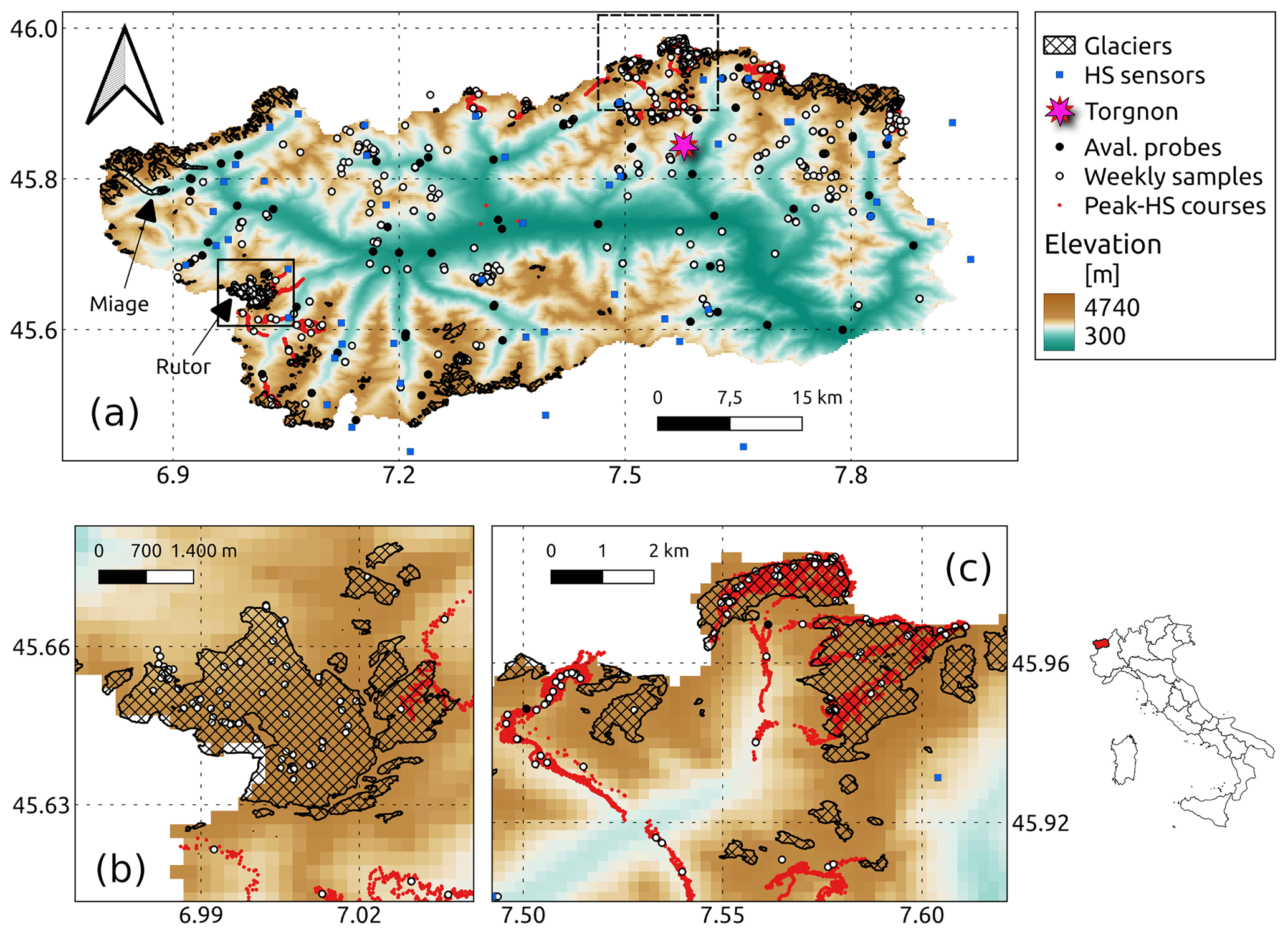
Figure 3 The Aosta Valley in northwestern Italy. (a) Topography and glaciology of this region, with locations of all snow-evaluation data used in this paper. (b, c) Zoom on two intensive measurement regions, the Rutor glacier and the headwaters of the Valpelline catchment, respectively. “HS sensors” are continuous-time snow-depth ultrasonic sensors, “Torgnon” is an intensive study plot with a variety of snow and weather datasets (see Sect. 3.3 and Terzago et al., 2019), “Aval. probes” denotes locations of snow-depth measurements for avalanche forecasting purposes, “Weekly samples” denotes locations of ∼ weekly snow-depth measurements collected mainly for water-supply forecasting, and “Peak-HS courses” is snow-depth measurements collected along transects of several kilometers for hydropower-forecasting purposes (see Avanzi et al., 2021, for more details). Panel (a) includes the locations of the Miage and Rutor glaciers, for which detailed evaluation results are reported in Sect. 3.5.

This section presents an application of S3M for an inner-Alpine valley located in northwestern Italy (Aosta Valley, Fig. 3). This area has steep elevation gradients, with the main valley at elevations on the order of 300–400 m a.s.l. and peaks as high as 4800 m a.s.l. (Mont Blanc) or 4478 m a.s.l. (Matterhorn). About 4 % of the Aosta Valley is covered by glaciers (134 km²), some of which are characterized by thick debris and extend over several kilometers (e.g., the Miage Glacier in the Mont Blanc massif). With its cryosphere-dominated water supply and complex precipitation–topography interactions leading to marked rain shadows (Avanzi et al., 2021), the Aosta Valley is a formidable test bed for S3M.

S3M has been operational in the Aosta Valley since the early 2000s as a component of a flood-forecasting chain called Flood-PROOFS (see Laiolo et al., 2014; Avanzi et al., 2021, and Sect. 2). This chain includes algorithms to spatialize and downscale weather-input data of precipitation, air temperature, relative humidity, and radiation, automatically generate daily maps of snow depth and use MODIS snow-covered area, and process independently derived weekly maps of SWE (see the Supplement). Together with runs of S3M in assimilation mode at ∼240 m spatial resolution, these tools inform real-time forecasts of streamflow at relevant closure sections (Laiolo et al., 2014; Avanzi et al., 2021). Details about spatialization techniques and hydrologic modeling in Flood-PROOFS are available elsewhere (Boni et al., 2010; Laiolo et al., 2014; Avanzi et al., 2021) and are not discussed here for brevity. In the present paper, we instead leverage our application in the Aosta Valley to provide guidelines on how to calibrate S3M in a real-world case study (Sect. 3.1) and how to validate and interpret model results for the snow (Sect. 3.2 to 3.4) and the glacier component (Sect. 3.5).

3.1 Calibrating S3M

S3M parameters that can be calibrated include the radiation and temperature snowmelt parameters $m_{\mathrm{rad}}^{\prime }$ and m_r, the threshold temperature for inhibiting snowmelt (T_τ), the maximum weight of SWE-assimilation maps (W), as well as a number of climatological thresholds used to constrain model predictions (e.g., maximum and minimum snow density or the snow-quality threshold to enable data assimilation; see the Supplement). While previous work from the author team in the Aosta Valley has involved calibration of many of the above parameters, the two melt parameters, $m_{\mathrm{rad}}^{\prime }$ and m_r, remain the prime calibration parameters of this model – like many other snowmelt models (Hock, 2003; Pellicciotti et al., 2005).

Because S3M is employed in assimilation mode in the Aosta Valley and this mode includes MODIS snow-covered area, our calibration rationale focused on maximizing fit for point predictions rather than for spatial patterns. Still, calibration was performed considering open-loop simulations to avoid model performance being spuriously driven by assimilation rather than parameter values. Calibration data comprised spatially distributed continuous-time measurements of 53 snow-depth sensors and temporally discontinuous manual measurements of snow depth collected across the region for water-supply or avalanche forecasting (see Avanzi et al., 2021, and Fig. 3 for a data inventory). The calibration period covered water years 2010 through 2019, where the bulk of the data was concentrated; the water year is a period between 1 September and 31 August and is indicated with the calendar year when it ends.

Our calibration protocol was based on performing multi-year simulations of S3M for a range of values of $m_{\mathrm{rad}}^{\prime }$ and m_r: [0.8, 2] and [0.5, 1.5] mm ^∘C⁻¹ d⁻¹, respectively. These ranges were chosen based on the fact that $m_{\mathrm{rad}}^{\prime }\sim \mathrm{1.1}$ implies a 100 % efficiency of transmitted shortwave radiation in generating melt under likely isothermal conditions (${\stackrel{\mathrm{‾}}{T}}_{\mathrm{10}\mathrm{d}}\to \mathrm{10}$ ^∘C; see Fig. 2a and Sect. 2), while m_r∼1.4 tallies with previous work by Pellicciotti et al. (2005). The parameter space was explored for increments of 0.025 of $m_{\mathrm{rad}}^{\prime }$ and 0.05 mm ^∘C⁻¹ d⁻¹ of m_r, and we first calibrated an optimal value of $m_{\mathrm{rad}}^{\prime }$ and then of m_r. This meant running 29 decade-long simulations for all tentative values of $m_{\mathrm{rad}}^{\prime }$, finding the optimal one, and then re-running 25 simulations tuning m_r. This sequential calibration approach is only one out of several possible calibration approaches, including strategically exploring the parameter space (Razavi et al., 2019). Here, we chose a sequential approach for this illustrative case study, mainly for computational-resource constraints.

As an objective metric, we minimized $\text{Obj}\left(\mathrm{\Theta }\right)=\mathrm{0.5}\times (\mathrm{1}-\mathrm{KGE}(\mathrm{\Theta }\left)\right)+\mathrm{0.5}\times \left(\mathrm{RMSE}\right(\mathrm{\Theta }\left)\right)/\stackrel{\mathrm{‾}}{\mathrm{RMSE}\left(\mathrm{\Theta }\right)}$, with Θ being the generic parameter value, KGE being the Kling–Gupta efficiency metric as defined in Kling et al. (2012), RMSE being the root mean square error, and $\stackrel{\mathrm{‾}}{\mathrm{RMSE}\left(\mathrm{\Theta }\right)}$ being the mean RMSE across all parameter values. This objective metric was chosen to combine the features of KGE (and in particular its focus on correlation, bias, and ratio of coefficients of variation) with a specific weight for large errors (RMSE). The RMSE was normalized by its mean across all parameter values to make it a-dimensional and so comparable to KGE. For each parameter value Θ, Obj was computed between observed snow depth (Fig. 3) and simulated h_S, both merging all data from all years into one sample and separately for each water year (all-year and yearly values, respectively).

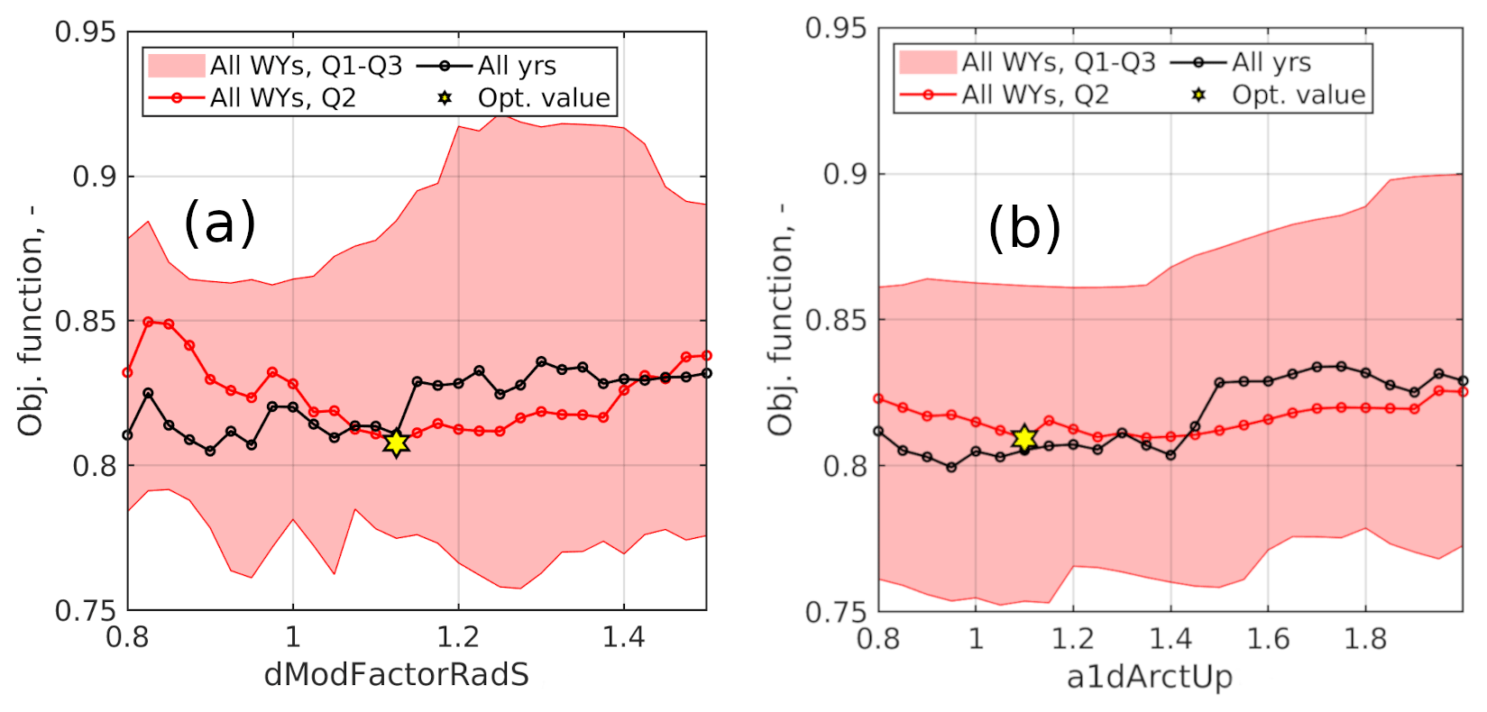
Figure 4 Calibration objective metrics as a function of parameter values, with dModFactorRadS being $m_{\mathrm{rad}}^{\prime }$ and a1dArctUp being m_r (see the Supplement for details on the model's notation in the source code). Parameter $m_{\mathrm{rad}}^{\prime }$ is a-dimensional, and m_r is in mm ^∘C⁻¹ d⁻¹. For each parameter value Θ, the objective metric was computed using both all data from all years in one sample and separately for each water year (all-year and yearly values, respectively). Q1, Q2, and Q3 are the first, second, and third quartiles of objective metrics across all water years. WY is water year.

Figure 5 Performance of S3M in simulating point snow depth, as measured by continuous-time snow-depth sensors (a), the snow-depth sensor at the intensive study plot of Torgnon, and manual snow-depth measurements taken for avalanche, hydropower, and water-supply forecasting (c–e). Because simulations were carried out in assimilation mode, and assimilated maps indirectly involved snow-depth sensors and weekly snow samples; performances for these datasets are reported only for reference. Panel (f) shows the elevation distribution of each dataset and of the Aosta Valley for context. RMSE is root mean square error, KGE is the Kling–Gupta efficiency (Kling et al., 2012), and r is Pearson's correlation coefficient. The spatial resolution of snow courses (d) is much finer than that of the model (say, ∼60 m vs. ∼220 m, respectively), and thus a number of snow-course data were compared to the same modeling value. This explains the occurrence of sharp, horizontal lines in panel (d).

Median yearly values across all water years show a minimum for $m_{\mathrm{rad}}^{\prime }=\mathrm{1.125}$ and then m_r=1.10 mm ^∘C⁻¹ d⁻¹, in line with expectations (Fig. 4 and Sect. 2). Objective-metric values showed remarkable variability across water years (see the quartile range in Fig. 4), owing to significant variability in the original sample of snow-depth values between warm and cold years (Avanzi et al., 2021). Thus, multi-year calibration periods are recommended, although the range of variability in median and all-year Obj in Fig. 4 suggests that the sensitivity of S3M to $m_{\mathrm{rad}}^{\prime }$ and m_r is low, especially if one considers that calibration-based snow models are prone to large drops in performance outside the calibration sample (Hock, 2003; Avanzi et al., 2016). We interpret this to be because of the hybrid physics-based and temperature-index approach employed in S3M to predict snowmelt (Eq. 15), which appears to better constrain parameter values than a purely temperature-index approach because it brings S3M closer to a first-principle energy balance model.

3.2 Evaluation: point snow depth

Figure 5 shows simulated vs. observed snow depth (symbol HS per guidelines by Fierz et al., 2009) for the 52 snow-depth sensors in Fig. 3, the snow-depth sensor at the Torgnon study plot, as well as for all manual snow-depth measurements taken for avalanche, hydropower, and water-supply forecasting (panels a to e, respectively). The evaluation period in Fig. 5 is water years from 2004 to 2009 and 2020, that is, all years before and after the calibration period in Sect. 3.1. Simulations in this and the following sections were carried out in assimilation mode, as this is the approach we generally use in real-time forecasting, and so results are more representative of real-world model performance. More details on this assimilation procedure are reported in Avanzi et al. (2021); note that assimilation is not performed between May and July to avoid interferences with the simulation of the depletion phase of the seasonal snowpack.

Snow-depth-sensor and weekly-snow-sample measurements in Fig. 5a and e were indirectly assimilated in S3M as they are involved in the computation of the so-called updating and weekly SWE maps (see Sect. 2), meaning their performance statistics are only reported for reference. Non-assimilated data at Torgnon (Fig. 5b) and from avalanche probes (Fig. 5c) maintain comparatively low and high values of RMSE and KGE, respectively (12–37 cm and 0.66–0.72, respectively), with no evident tendency for systematic underestimations or overestimations. Open-loop results were not reported here for brevity but generally show comparable performance for these datasets. Thus, we conclude that our calibration strategy not only showed little sensitivity of the model to $m_{\mathrm{rad}}^{\prime }$ and m_r (Fig. 4), but also led to a robust performance across nearly 20 water years and for areas that were not included in the calibration pool.

Peak-snow-depth courses show a significantly lower performance, in particular in terms of a larger dispersion around the 1:1 line, a larger RMSE (122 cm), and a lower KGE (0.57, Fig. 5d). This is because this course dataset comprises snow-depth measurements at significantly higher elevations than any other considered dataset (see the elevation distribution in Fig. 5f). At those elevations, both interactions between the snowpack and topography complicate snow distribution compared to low-elevation areas, and density of input-data stations is much lower (Avanzi et al., 2021). Still, the fact that S3M does not show any obvious overestimation or underestimation for those elevations is encouraging for our scopes, also considering the comparatively coarse resolution of our implementation in the Aosta Valley (∼240 m).

Figure 6 Comparison between measurements and modeling outputs at the Torgnon study plot. The first, second, third, and fourth columns are snow depth (HS), SWE, bulk-snow density, and albedo, respectively. The third and fourth columns also report dry-snow density and bulk volumetric liquid-water content, respectively. Each row is one water year (2013 to 2020). “OL” and “Assim.” stand for open-loop and assimilated simulations, respectively.

3.3 Evaluation: the Torgnon study plot

S3M reproduces the timing of peak accumulation and so the onset of the snowmelt season in the Torgnon study plot in terms both of snow depth (h_S) and SWE (Fig. 6; this figure includes a mixture of calibration – 2013–2019 – and evaluation – 2020 – water years). In this regard, Kling–Gupta efficiency for snow depth and SWE is ∼0.70 and ∼0.84, respectively. Discrepancies between observed and simulated snow depth increase in spring, mainly because spatial heterogeneity in snow depth increases during the snowmelt season (Grünewald et al., 2010), and this challenges the comparison between a point measurement of snow depth and our 240 m snow model. Overall, the model correctly captures snowmelt rate and peak SWE for most water years, which are the primary variable of interest in operational snow hydrology.

Sporadic yet abrupt oscillations in snow depth or SWE in the assimilated simulation are due to the assimilation dataset, which is the operational result of a multi-regression model fitted across observed snow depth at ultrasonic-sensor stations and a number of physiographic features (Avanzi et al., 2021). These regressions often maintain – or even propagate – measurement noise, a frequent issue of ultrasonic snow-depth sensors (Ryan et al., 2008). Open-loop simulations do not display the same abrupt oscillations, which validates a model's parametrizations.

S3M also reproduces the magnitude of bulk-snow density and its increase with time for all water years (Fig. 6), in agreement with previous models implementing a similar parametrization of snow settling (De Michele et al., 2013; Avanzi et al., 2016) and despite its one-layer approach. Values of bulk and dry snow density are very close to each other during the accumulation season, while the latter diverges from the former during the snowmelt season. This is due to an increase in mass for the wet component of the snowpack during spring, as confirmed in terms of bulk liquid-water content (Fig. 6). The seasonal range of variability for modeled bulk liquid-water content and its peak around 5 vol % during the snowmelt season agree with measurements by Techel and Pielmeier (2011), Heilig et al. (2015), Avanzi et al. (2017) and the international classification by Fierz et al. (2009).

The Torgnon study plot also measures incoming and reflected shortwave radiation, which allowed a comparison in terms of measured and simulated albedo (Fig. 6). During the accumulation season, measured albedo is generally higher than simulated albedo; in particular, both measured and simulated albedos show maximum values around 0.95, but only the latter decreases well below 0.8–0.7 between snowfall events. Simulations by SNOWPACK at the same study plot (Terzago et al., 2019, not reported for brevity) qualitatively showed higher values than S3M, evidence that only relying on time as a predictor of albedo may yield frequent underestimations compared to a model that considers a broader spectrum of albedo predictors like SNOWPACK. On the other hand, S3M well captures the measured decline in albedo during the snowmelt season, which, again, is important for capturing the timing and intensity of seasonal melt.

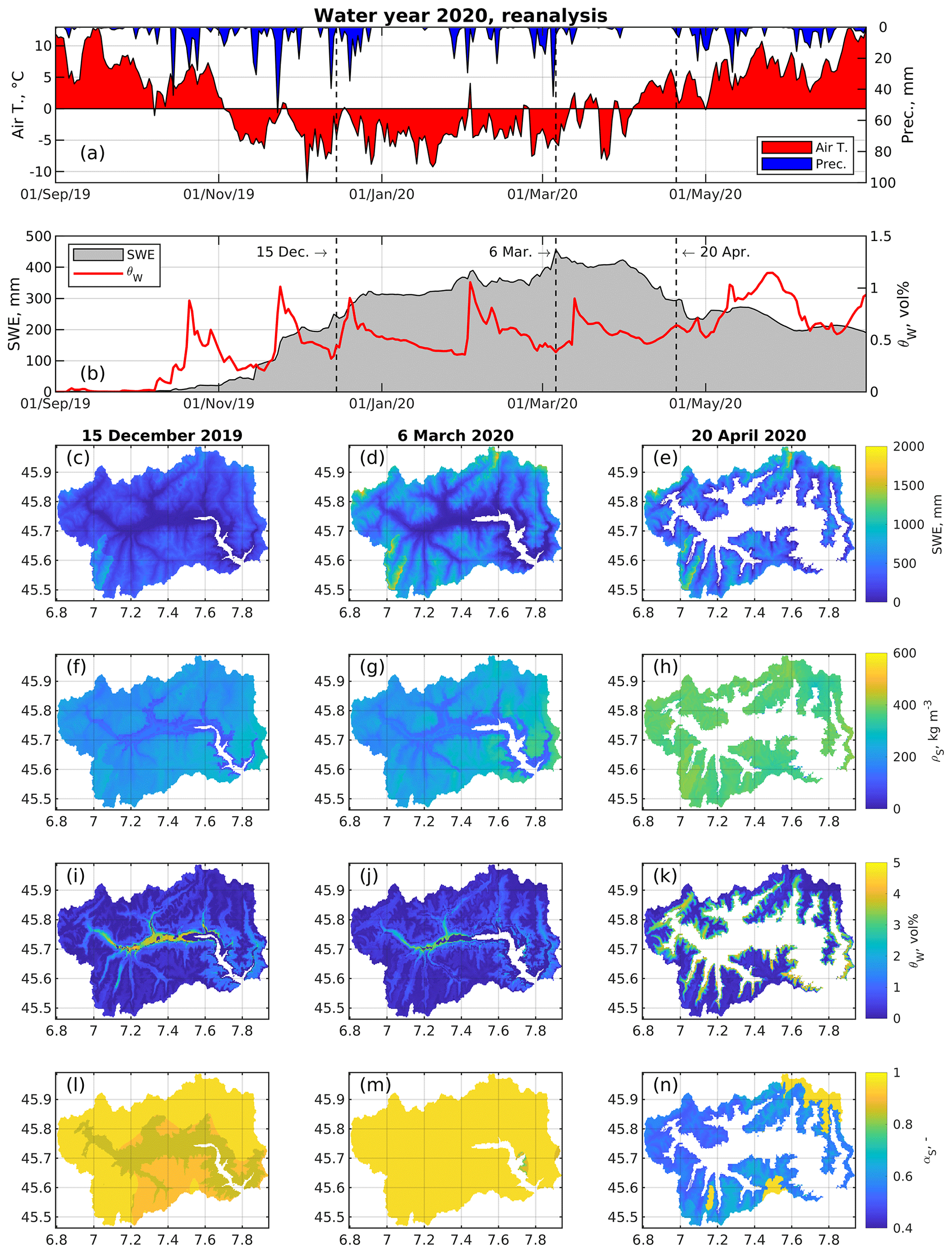
Figure 7 Simulated reanalysis of the 2020 snow season: spatially averaged air temperature and total precipitation (a), spatially averaged SWE and bulk liquid-water content θ_W (b), and distribution of SWE (c–e), bulk snow density ρ_S (f–h), bulk liquid water content (i–k), and albedo α_S (l–n) for three example dates: 15 December 2019 (first column), 6 March 2020 (middle column), and 20 April 2020 (third column). Statistics in panels (a) and (b) are spatial averages across the entire Aosta Valley region.

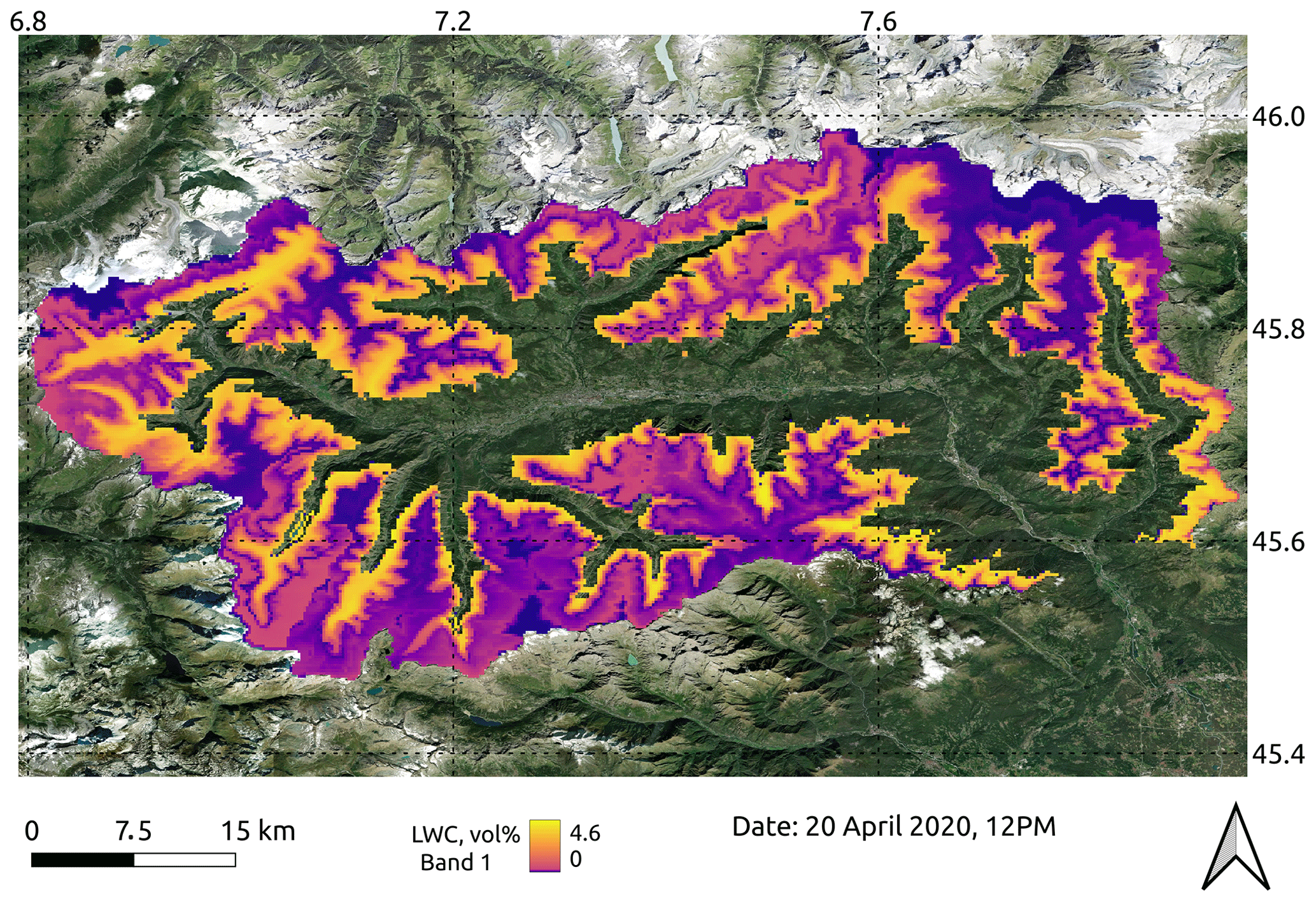
Figure 8 Map of bulk volumetric liquid-water content for the Aosta Valley (LWC, same as θ_W), 20 April 2020 at 12:00. The background layer is from the ESRI satellite theme.

3.4 Evaluation: snow distribution

Figure 7 shows a simulated reanalysis of the 2019–2020 snow season, which exemplifies the information and level of detail provided by S3M to forecasters (note that this snow season is part of the validation pool). The 2020 snow season started by the end of October 2019 (Fig. 7a), with largely uninterrupted precipitation events between November and December 2019 leading to nearly 75 % of spatially averaged SWE across the Aosta Valley being accumulated before January 2020 (Fig. 7b). January and February were relatively dry months, with only one storm in mid-February and then another one between February and early March 2020. The snowmelt season started in April, even though ∼40 % of spatially averaged SWE at high elevations persisted by the end of May 2020. The season was characterized by an alternation between cold and warm spells, which led to frequent melt–freeze cycles in the spatially averaged snowpack (Fig. 7b).

The spatial distribution of SWE confirmed an increase in snow accumulation between 15 December (Fig. 7c) and 6 March (Fig. 7d), with the expected positive gradient with elevation. Simulations for 20 April 2020 showed a typical snapshot of the snowmelt season, with largely depleted snowpack at low and medium elevations and SWE still on the order of 1000–1500 mm at elevations above 3000 m a.s.l.

Bulk-snow density was spatially fairly homogeneous, especially at the beginning of the snow season (Fig. 7f). With time, some differences emerged, with snow density increasing faster in areas with both larger SWE and likely warmer temperatures (Fig. 7g and h). Both the magnitude of snow-density values in Fig. 7 and the fact that this variable was spatially more homogeneous than SWE tally with previous works (López Moreno et al., 2013).

Maps of bulk-liquid water content were largely influenced by local climate, with a general rise in wetness with decreasing elevation that closely followed local topographic contours and aspect (Fig. 7i to k and Fig. 8). Overall, bulk liquid-water content around the snow line was larger in April than in December or March, which again tallies with expected seasonal trends in wetness (Techel and Pielmeier, 2011). While liquid water in snow has been investigated for a long time (Colbeck, 1971), recent work on wet snow provides new opportunities for considering bulk liquid-water content from an operational standpoint, whether to predict the onset of snowpack runoff (Wever et al., 2014) or wet-snow avalanches (Mitterer et al., 2013; Wever et al., 2016). Early evidence that wet-snow conditions have increased in frequency and have extended well into the winter season due to a warming trend (Pielmeier et al., 2013) further justifies interest in wet-snow predictions like those in Fig. 8. While application to significantly changed conditions will necessarily require some forms of parameter tuning or recalibration, S3M is among the few parsimonious snow models to provide spatially explicit, raster-like predictions of wet-snow patterns.

Maps of albedo showed the expected homogeneity during the accumulation season, owing to frequent snowfall events between November and March (Fig. 7l and m). On the other hand, albedo in spring was much lower and spatially more diverse than in winter, with values larger than 0.8 at high elevation and values well below 0.6–0.7 in areas covered by older and wetter snow.

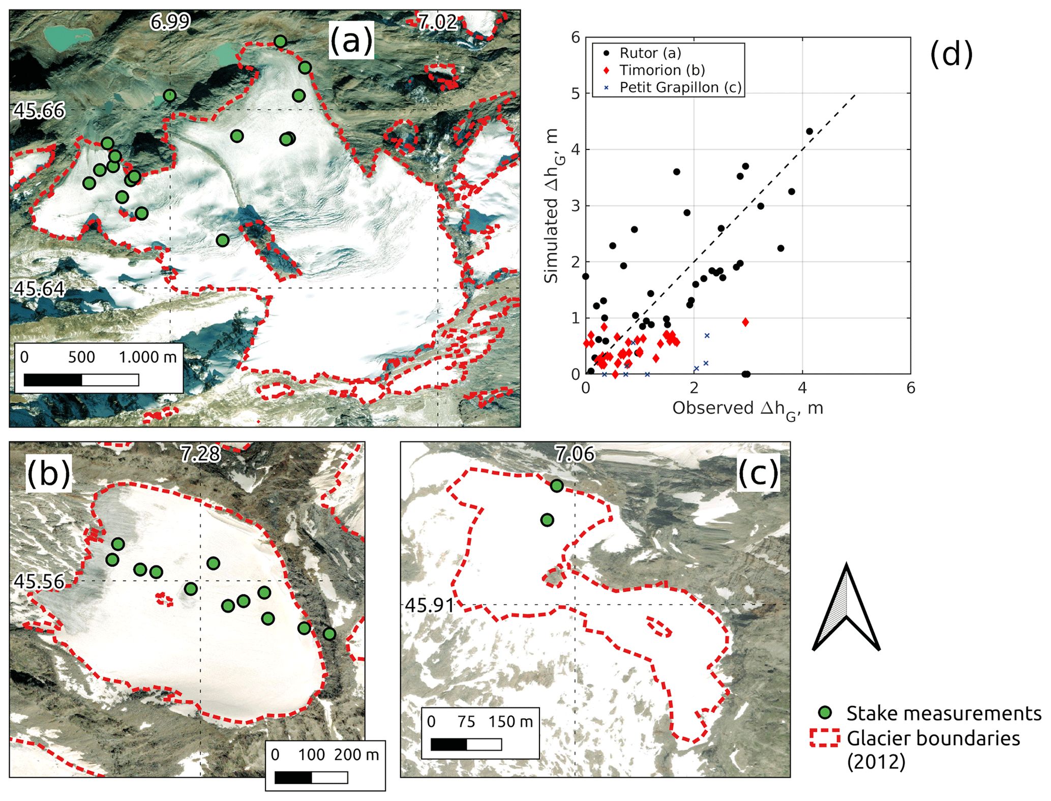
Figure 9 Spatial distribution of glacier-ablation measurements across the Rutor (a), the Timorion (b), and the Petit Grapillon (c) glaciers in the Aosta Valley. Panel (d) shows a comparison between measured and simulated ablation (positive values mean a decrease in local ice thickness). The number of points in panel (d) does not correspond to the number of stake locations in panels (a) to (c) because of repeated measurements taken across multiple water years as the same stake location. The background layer is from the ESRI Satellite theme.

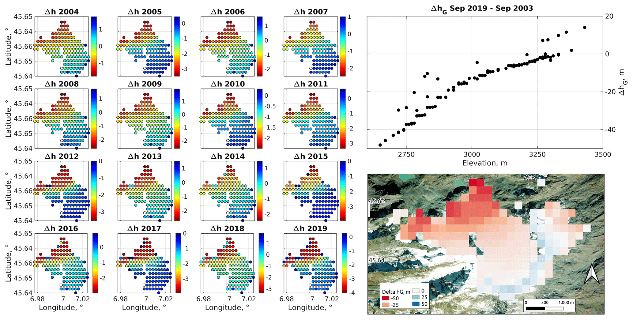
Figure 10 Rutor glacier: spatial patterns of annual change in glacier thickness (left), cumulative change in glacier thickness between September 2003 and 2019 as a function of pixel elevation (right, top), and spatial distribution of this cumulative change (right, bottom). The background layer is from the ESRI Satellite theme.

Figure 11 Miage Glacier: spatial patterns of annual change in glacier thickness (left), cumulative change in glacier thickness between September 2003 and 2019 as a function of pixel elevation (right, top), and spatial distribution of this cumulative change (right, bottom). The background layer is from the ESRI Satellite theme.

3.5 Evaluation: glacier evolution

To evaluate the glacier component of S3M in the Aosta Valley, we considered 94 ablation-stake measurements across the Rutor, Timorion, and Petit Grapillon glaciers (period 2009–2015, Fig. 9). These are all high-elevation, debris-free glaciers of various sizes (7.91, 0.48, and 0.18 km², respectively – 2012 data from the Aosta Valley Environmental Protection Agency), thus providing a representative sample to test the accuracy of S3M in capturing glacier ablation (note that these measurements were not included in the calibration of S3M, so they are a validation dataset).

Simulations using the G3 glacier module (that is, including the Δh parametrization) returned a correlation between simulated and observed change in thickness of 0.6 (Fig. 9d). The correspondence between simulated and observed change in thickness across the range of variability in measurements was higher for Rutor than for Timorion and Petit Grapillon, which we interpret because of the large size of the former compared to model resolution (240 m). Also, the number of available samples for Rutor is significantly larger than for Timorion and Petit Grapillon; for the latter, glacier surveys are challenged by extensive and deep crevasses as well as frequent avalanches that make point measurements non-representative of the actual melt pattern. Thus, the performance observed for the Rutor glacier is more representative of S3M predictive skills.

The evolution of glacier thickness for the Rutor glacier shows expected spatial patterns, with minor ablation at elevations above 3000 m a.s.l. and progressively more intense melt close to the terminus below 2750 m a.s.l. (Fig. 10; see Fig. 3 for the location of this glacier in the study region). Annual changes show significant interannual variability, with somewhat more intense melt as the evaluation period progresses; in any case, the spatial pattern is preserved as hypothesized by the Δh parametrization. At elevations above 3200 m a.s.l., glacier thickness increased owing to conversion of seasonal snow to glacier ice at the end of the water year (see Sect. 2.6).

Figure 11 shows similar spatial patterns for one of the most complex glaciers in the Alps, the Miage Glacier, a 10.8 km² (2012), 10 km+-long valley glacier covering a ∼2000 m elevation range of the Mont Blanc massif (see Fig. 3 for the location of this glacier in the study region). Like many other valley glaciers across the southern Alps (Diolaiuti et al., 2003), vast portions of the Miage tongue are covered by debris, which has been shown to lead to below-debris melt being insensitive to variations in atmospheric temperature (Brock et al., 2010). Albeit hard to validate due to a lack of measurements, our implementation of the Miage Glacier qualitatively captured this disconnection between intense melt across medium-elevation areas with little to no known debris and low melt rates in areas close to the glacier terminus that are well known to be covered by thick debris (Fig. 11). Thanks to supporting a spatially explicit debris-driven melt factor (Eq. 40), S3M yielded estimates of thickness change that were more spatially diverse and less correlated with elevation on the Miage Glacier than on the Rutor glacier (correlation coefficients of 0.95 and 0.85, respectively; compare Fig. 11 with Fig. 10). At elevations above ∼3000 m a.s.l., debris is residual if non-existent, and so change in thickness and elevation maintained the same high correlation observed on the Rutor glacier in Fig. 10.

4 Applicability and future developments

As a hydrology-oriented cryospheric model, S3M delivers timely and computationally efficient predictions while aiming at including the most salient processes of snow and glacier hydrology. Understanding this trade-off and its implications is important for determining model applicability and adequacy in a given context.

The structure and state variables of the model are all geared toward providing decision-relevant information for water-supply forecasting, which remains the prime area of application tested by the authors (Laiolo et al., 2014). In this context, typical questions that S3M contributes to answering are how many snow-water resources are currently accumulated across the landscape, which headwater regions are currently releasing meltwater and which are still accumulating snowpack, when a certain percentage of the seasonal freshet is expected to reach a given closure section, and whether glaciers are currently contributing runoff and if so how much their relative contribution is. Decisions that are currently being informed by S3M thus range from flood-forecasting early warning to hydropower planning. S3M also provides some support to avalanche hazard forecasting, but this remains an unexplored area of application for which the microstructural detail in this model is largely insufficient.

Recently, we also started using S3M to produce future scenarios of water resources in mountain regions. Two particular features of S3M in this regard are the comparatively limited computational times of this model and the inclusion of both snow and glacier mass balances. Regarding the former, computational time for 1 water year worth of simulations in the Aosta Valley is ∼1.5 h for a laptop with six i7 eighth-generation cores and solid-state storage (240 m resolution, ∼3290 km²). Note that S3M includes access to and creation of input and output NetCDF files (see the Supplement), and the frequency and size of output files in particular play an important role in determining computational time. Regarding snow and glacier mass balances, models providing even medium-level physical realism of both these features are still rare (Bongio et al., 2016; Li et al., 2015). Thanks to its integration with the Continuum hydrologic model (also open source; see Silvestro et al., 2013), S3M can deliver mass-conserving and spatially consistent predictions of the entire mountain water budget.

S3M is currently being actively maintained and further developed, with five main areas of planned future work. The first is the inclusion of wind effects, both as an additional component of the energy balance and as a driver of snow redistribution (wind drift). Explicitly including wind in the energy budget will help to resolve rain-on-snow events in the model, given that turbulent fluxes are a key contributor to melt during such flood-generating events (Marks et al., 1998; Würzer et al., 2016). As for wind drift, advances in this context are warranted not only in terms of relocation of blowing snow in the form of suspension, saltation, and creep (DeWalle and Rango, 2011), but also (and likely more importantly) in terms of the associated sublimation. Progress in this regard has been hampered by a lack of detailed measurements of wind across the complex terrain of mountain headwaters, but recent datasets in this regard may favor future work on this topic (Guyomarc'h et al., 2019).

A second area of planned future work regards the inclusion of vegetation effects on the snowpack. The science of canopy–snow interactions has identified four mechanisms through which vegetation can alter snowpack evolution compared to open areas: precipitation interception and throughfall, shortwave radiation shadowing, longwave-radiation enhancement, and wind shielding (Rutter et al., 2009). While the importance of each of these mechanisms for the fate of a seasonal snowpack dramatically changes with local climate (Lundquist et al., 2013), scientific consensus is that canopy may reduce peak SWE by more than 50 % and lead to perturbations in the melt-out date on the order of weeks (Rutter et al., 2009), depending on canopy or snow-fractional cover. Helbig et al. (2020) and Mazzotti et al. (2021) have recently proposed a parsimonious parametrization for canopy effects in large-scale models, thus providing a solid starting point to include these processes in S3M.

The third direction of future development is liquid-water transport in snow, a rarely parametrized but important connection between surface melt and snowpack runoff. Water infiltration through snow manifests itself as both spatially homogeneous matrix flow and spatially heterogeneous preferential flow (Katsushima et al., 2013), with transitions between these two regimes being driven by wet-snow metamorphism and snow properties like density and grain size (Avanzi et al., 2017; Hirashima et al., 2019). While capturing such micro-scale mechanisms is beyond the scope of a large-scale, distributed model, including some forms of preferential flow in S3M will likely enhance its performance in terms of timing and peak of early-season snowmelt events or rain on snow (Wever et al., 2014; Würzer et al., 2017). A way forward in this regard may be the simple parametrization originally proposed by Katsushima et al. (2009), which models preferential-flow discharge as a θ_W-driven threshold process. Another important aspect here is slope flow, that is, the tendency of snow to redistribute meltwater along layer boundaries for distances of hundreds of meters downhill (Eiriksson et al., 2013; Webb et al., 2018). Both measurements and consequently parametrizations of this process are still very rare, and more work is needed before this process can be included in parsimonious models like S3M.

Fourth, the conversion from snow to ice in S3M is very simplified and completely skips the intermediate stage of firn (Cuffey and Paterson, 2010). While we usually turn off the glacier-mass balance when using S3M in flood forecasting and while accumulation of multi-year snow as firn will likely characterize only very high elevations in a warming climate, this transition is still an important process for capturing from the perspective of physical realism. Considering firn may also extend the applicability of S3M to polar regions, where for example firn-storage capacity is an important factor in determining the long-term fate of the Greenland ice sheet (Forster et al., 2014; Machguth et al., 2016). In this regard, Banfi and De Michele (2022) have recently proposed a local model of snow–firn transition for a binary-mixture snowpack like that considered in S3M.

Fifth, more work is planned to improve the data-assimilation component of S3M, particularly in terms of widening the array of state variables for which assimilation is supported (currently, SWE and snow depth) and in terms of improving assimilation data themselves. Regarding the former, the field of multivariate data assimilation is ripe (Piazzi et al., 2018), although scaling up these approaches across the landscape may come with significant computational requirements. Regarding new assimilation data, statistical learning is making promising steps towards mining new information from traditional, sometimes even sparse and fuzzy data across geosciences (Avanzi et al., 2019; Ghanjkhanlo et al., 2020; Revuelto et al., 2020; Dramsch, 2020; Grossi et al., 2021; Maurer et al., 2021; Shen et al., 2021; Mosaffa et al., 2022). Meanwhile, Cluzet et al. (2020) have shown some degree of success in assimilating satellite reflectance into snowpack simulations as a way to better capture snow microstructure and so the energy balance. Lessons learned from these recent advances will be incorporated into future releases of S3M.

5 Conclusions

We presented S3M v5.1, a spatially explicit hydrology-oriented cryospheric model that successfully reconstructs seasonal snow and glacier evolution through time. The model comprises parametrizations for precipitation-phase partitioning, snow and glacier mass balances, snow rheology and density evolution, snow aging and albedo, a hybrid temperature-index and radiation-driven melt parametrization, and provisions for data assimilation. Through a case study in the Aosta Valley, we showed that S3M provides robust performance across nearly 20 water years, with no systematic overestimation or underestimation of snow depth and a satisfactory simulation of the timing of peak accumulation and so the onset of the snowmelt season, including the transition from dry to wet snow (root mean square errors between S3M-simulated snow depth and in situ measurements between ∼12 and ∼120 cm depending on elevation, with Kling–Gupta efficiencies between 0.55 and 0.82).

Overall, the model channels elements from the state of the art in cryospheric sciences into a parsimonious and computationally efficient model. Regarding snow, specific elements of relative novelty in this regard are an explicit representation of snow liquid-water content and a hybrid physics-based and temperature-index approach to snowmelt that decouples the radiation- and temperature-driven contributions. The glacier component also includes the well-known Δh parametrization and the possibility of feeding the model with a distributed debris-driven melt factor, both comparatively new approaches in the field.

S3M provides an open-source platform to simulate snow and glacier dynamics with the necessary physical realism for hydrologic purposes. Together with the Continuum hydrologic model (Silvestro et al., 2013), S3M fulfills the recurring need for integrated glacio-hydrologic models in both scientific research and operational practice and can provide the basis for more robust, large-scale predictions of the fate of the cryosphere at multiple timescales – from hours to centuries ahead.