the Creative Commons Attribution 4.0 License.
the Creative Commons Attribution 4.0 License.
 | 09 May 2022
Blockworlds 0.1.0: a demonstration of anti-aliased geophysics for probabilistic inversions of implicit and kinematic geological models
Richard Scalzo
Mark Lindsay
Mark Jessell
Guillaume Pirot
Jeremie Giraud
Edward Cripps
Sally Cripps
Parametric geological models such as implicit or kinematic models provide low-dimensional, interpretable representations of 3-D geological structures. Combining these models with geophysical data in a probabilistic joint inversion framework provides an opportunity to directly quantify uncertainty in geological interpretations. For best results, care must be taken with the intermediate step of rendering parametric geology in a finite-resolution discrete basis for the geophysical calculation. Calculating geophysics from naively voxelized geology, as exported from commonly used geological modeling tools, can produce a poor approximation to the true likelihood, degrading posterior inference for structural parameters. We develop a simple integrated Bayesian inversion code, called Blockworlds, showcasing a numerical scheme to calculate anti-aliased rock properties over regular meshes for use with gravity and magnetic sensors. We use Blockworlds to demonstrate anti-aliasing in the context of an implicit model with kinematic action for simple tectonic histories, showing its impact on the structure of the likelihood for gravity anomaly.
- Article
(6501 KB) - Full-text XML
- BibTeX
- EndNote


Geological modeling of subsurface structures is critical to decision-making across numerous application areas, including mining, groundwater, resource exploration, natural hazard assessment, and engineering, yet is also subject to considerable uncertainty (e.g., Pirot et al., 2015; Linde et al., 2017; Witter et al., 2019; Quigley et al., 2019; Wang et al., 2020). Uncertainty arises in numerous places within the model-building workflow, including sparse, noisy, and/or heterogeneous geological observations and rock property measurements; the indirect nature of geophysical measurements; the non-uniqueness of inverse problem solutions; and the ambiguity of geological interpretations (Lindsay et al., 2013). Rigorous quantification of uncertainty is therefore critical to decision-making informed by models, and is becoming an increasingly active area of research in geology and geophysics (Rawlinson et al., 2014; Bond, 2015; Jessell et al., 2018; Wellmann and Caumon, 2018).
Bayesian methods provide a probabilistically coherent framework for reasoning about uncertainty (Tarantola and Valette, 1982; Mosegaard and Tarantola, 1995; Mosegaard and Sambridge, 2002). Although not the only way to account for uncertainty in earth science settings, Bayesian reasoning enables the natural integration of heterogeneous data and expert knowledge (Jessell et al., 2010; Bosch, 2016; Beardsmore et al., 2016), guides the acquisition of additional data for maximum information gain (e.g., Pirot et al., 2019b), enables selection among competing conceptual models (e.g., Brunetti et al., 2019; Pirot et al., 2019a), and optimizes management of risk in decision-making over possible outcomes (e.g., Varouchakis et al., 2019).
Bayesian methods are used in both geology and geophysics, but with different framing for inference problems. In the geophysics community, where quantitative inversion frameworks have been in use for decades (Backus and Gilbert, 1967, 1968, 1970), the core problem is framed as a nonparametric imaging of the subsurface. The model parameters directly define discretized spatial fields of rock properties, from which forward geophysics are calculated to reproduce observations. Model structures rich enough to be useful are often very high-dimensional, and variations in spatial scales and resolutions make the full covariance matrix cumbersome and impractical to evaluate (Rawlinson et al., 2014). Although the discrete geophysical image representation may naturally reflect the geological interpretation (for example, in the transdimensional inversions reviewed in Sambridge et al., 2012), this is not usually the case, and much effort goes into developing models with priors or regularizing terms to constrain the outputs of geophysical inversions to be geologically reasonable. Examples include the hierarchical Bayesian “lithologic tomography” of Bosch (1999) and Bosch et al. (2001), structure-coupled multiphysics approaches (Gallardo and Meju, 2011; de Pasquale et al., 2019), and flexible models based on Voronoi tessellations or multi-point statistics (e.g., Cordua et al., 2012; Pirot et al., 2017). Level-set methods (Osher and Sethian, 1988; Santosa, 1996; Li et al., 2017; Zheglova et al., 2018; Giraud et al., 2021a) solve for the boundaries of discrete rock units; these methods are more parsimonious than traditional volumetric inversions but still invert for a flexible, high-dimensional description of static 3-D properties.
In contrast, the core problem in geology is to interpret observations in terms of geological histories and processes (Frodeman, 1995). This becomes important in the structural geology of ore-forming systems, where details of the history become important and flexible treatment of 3-D geological structures as random fields is inadequate (Wellmann et al., 2017). The mineral exploration community has developed 3-D geological forward models that can capture much of the complexity of real systems (e.g., Perrouty et al., 2014). Implicit models (Houlding, 1994) represent interfaces between geological units as isosurfaces of a scalar field defined over 3-D space. The popular industry software package 3D GeoModeller (Calcagno et al., 2008) and the open-source code GemPy (de la Varga et al., 2019) interpolate this scalar field directly from structural geological observations by co-kriging (Lajaunie et al., 1997). Kinematic models (Jessell, 1981) use a parametrized description of volume deformations produced by tectonic events; the open-source package Noddy (Jessell and Valenta, 1993) is commonly used. The recently released open-source package LoopStructural (Grose et al., 2020) combines elements of co-kriging and kinematic implicit models for additional geological richness and realism. For models with no constraints from geophysics, geological uncertainty can be quantified by generating Monte Carlo realizations (Metropolis and Ulam, 1949) of geological datasets (Pakyuz-Charrier et al., 2018a, b, 2019). In a Bayesian treatment, this amounts to drawing samples from the prior (Wellmann et al., 2017).
Conditioning geological forward models on geophysical observations makes it tractable to perform full posterior inference in an interpretable parameter space of reduced dimension. This can be done using sampling methods such as Markov chain Monte Carlo methods (MCMC; Metropolis et al., 1953; Hastings, 1970), which are becoming increasingly sophisticated and widely used in geological and geophysical modeling (Mosegaard and Tarantola, 1995; Mosegaard and Sambridge, 2002; Sambridge et al., 2012). Additionally, parametric geology naturally obeys constraints imposed by the forward geological process, and can be used for inference over that process, unlike nonparametric geophysical inversions that incorporate a static, voxelized geological model as a prior mean (Giraud et al., 2017, 2018, 2019a, b; Ogarko et al., 2021; Giraud et al., 2021b). Kinematic models are especially well suited for this approach since they represent geological hypotheses in terms of structural observations and event histories but avoid the full computational burden of dynamic process-based simulations. Performing Bayesian inference over kinematic model parameters could open the door to more general Bayesian model selection over geological histories or conceptual models.
Probabilistic inversion workflows that incorporate forward geophysics based on forward-modeled 3-D structural geology are, to date, still uncommon, owing in part to computational challenges faced by sampling algorithms. The pyNoddy code (Wellmann et al., 2016) provided a wrapper to Noddy to enable Monte Carlo sampling of 3-D block models and potential fields, but not posterior sampling of an inversion conditioned on gravity or magnetic data. The Obsidian distributed inversion code (McCalman et al., 2014) implemented a geological model of a layered sedimentary basin with explicit unit boundaries to explore geothermal potential (Beardsmore et al., 2016); it featured multiple geophysical sensors and a parallel-tempered MCMC sampler for complete exploration of multi-modal posteriors. Obsidian has been extended with new within-chain MCMC proposals inside the parallel-tempered framework (Scalzo et al., 2019) and a new sensor likelihood for field observations of surface lithostratigraphy (Olierook et al., 2020), but the limitations of its geological model make it an unlikely engine for general-purpose inversions. Wellmann et al. (2017) present a workflow that uses GeoModeller to render the geology, Noddy for calculation of geophysical fields, and pymc2 (Patil et al., 2010) for MCMC sampling. GemPy's support for information other than structural geological measurements is as yet fairly limited, but includes forward modeling of gravity sensors and topology.
This paper describes a simple Bayesian inversion framework, called Blockworlds, which to our knowledge is the first to perform full posterior inference based on forward geophysics from an implicit geological model with kinematic elements. Although not yet intended to serve as a production-ready geological modeling package, Blockworlds' design addresses an obstacle for inversion workflows that resample the parametrized 3-D geometry of geological units onto a discrete volumetric mesh for geophysical calculations. Discontinuous changes in rock properties across unit interfaces may become undersampled unless the mesh is chosen to align with those interfaces (Wellmann and Caumon, 2018); since implicit and kinematic geological models naturally represent geology volumetrically, this alignment is not easily made without first evaluating the model, incurring additional computational overhead. Flexible geophysical inversions can adjust rock properties in individual boundary voxels to partially compensate for the loss of accuracy, but models that condition rock properties directly on geological parameters lose much of this freedom. This can result in artifacts in the likelihood that hinder convergence of estimation methods, degrade posterior inference over structural parameters, and preclude the use of posterior derivative information.
To address the issue of undersampled interfaces, Blockworlds incorporates numerical anti-aliasing into its discretization step. Anti-aliasing to address undersampling has a long history in computer graphics (Crow, 1977; Catmull, 1978; Cook, 1986; Öztireli, 2020) and in geophysics, for example, finite-difference solutions of seismic wave equations (Backus, 1962; Muir et al., 1992; Moczo et al., 2002; Capdeville et al., 2010; Koene et al., 2021). Obsidian anti-aliases physical rock properties using volume averages in voxels with partial unit membership, though this is not mentioned in associated publications (McCalman et al., 2014; Beardsmore et al., 2016), and the implementation depends upon the Obsidian parametrization. Blockworlds' prescription is more general, operating on the scalar field values that define interface positions in all implicit models, and thus can be straightforwardly implemented for implicit models using other types of interpolation schemes such as co-kriging.
This paper is organized as follows. Section 2 explains the aliasing effect, including its influence on the likelihood, and describes the algorithm used in Blockworlds to address it. Section 3 describes how Blockworlds evaluates kinematic event histories, then introduces a set of synthetic kinematic geological models we use as benchmarks. Section 4 summarizes gravity inversion experiments based on these models, demonstrating the influence of anti-aliasing on MCMC sampling. Section 5 discusses future directions, including the use of anti-aliasing with other geophysical sensors and curvilinear coordinate systems, and we conclude in Sect. 6.
2.1 Chaining forward models in geophysics calculations from structural geology
The forward modeling of observations falls under the calculation of the likelihood p(d|θ), which describes the probability of observing data d given that the causal process generating the data has true parameters θ. A Bayesian inversion proceeds by combining the likelihood with a prior p(θ) that describes the strength of belief, in terms of probability, that the causal process has true parameters θ before any data are taken into account. In nonparametric geophysical inversions, the prior includes regularization terms that penalize undesirable solutions. In parametric inversions, the choice of parametrization corresponds to a strong regularization on the discretized geology, with the prior distribution providing further constraints. The posterior distribution p(θ|d), describing probabilistic beliefs about θ once the data have been taken into account, is then determined through Bayes's theorem:
For parameter estimation, the unnormalized right-hand side can then be sampled using MCMC algorithms for full uncertainty quantification.
While some measurements, such as structural observations, can be computed directly from a continuous functional form for the geological forward model, the calculation of likelihoods based on simulation of geophysical sensors may require discretization of the geology. The likelihood terms in this case each involve the composition of two forward models:
-
a mapping from the parameter space Θ into a space 𝒢 of discrete volumetric representations (such as block models); and
-
a mapping from the space of discretizations into the space of possible realizations of the data.
Structural geology is chiefly concerned with the map g, and often reckons uncertainty not in terms of parameter variance, but in terms of the properties of an ensemble of discrete voxelized models (e.g., Wellmann and Regenauer-Lieb, 2012; Lindsay et al., 2012). Inversions of geophysical sensor data such as gravity, magnetism, conductivity, or seismic data are chiefly concerned with the map f. The accuracy of a parametric inversion will depend on the accuracy with which f∘g can be computed.
Although discretization methods such as adaptive meshes (Rawlinson et al., 2014) or basis functions aligned with geological features (Wellmann and Caumon, 2018) can improve the fidelity of g, these mappings are not guaranteed to be suitable for efficient and accurate computation of f. Furthermore, existing geological engines frequently export to a simple fixed basis that may be adequate for visualization in an interactive workflow but causes trouble in automated inversion workflows, producing the aliasing effects discussed in the next subsection.
2.2 Aliasing and its effects on the posterior
To show a straightforward example, we calculate the posterior density for the parameters of a uniform-density spherical inclusion (sphere radius and mass density) given the gravitational signal. An analytic solution exists, so we can compare directly to the true posterior, and with only two parameters we can simply evaluate over a grid of parameter values rather than using MCMC. We model a 1 km3 cubical volume, and fix the sphere's position at the center. Gravity anomaly data were generated from the analytic model on an evenly spaced 20×20 survey grid at the surface (z=0), with Gaussian measurement noise at the level of 10 % of the signal amplitude added. We used version 0.14.0 of the SimPEG library (Cockett et al., 2015; Heagy et al., 2020) to generate meshes and calculate the action of the forward model for the gravity sensor in the inversion loop. To emphasize the role of the likelihood in a scenario with vague prior constraints, we use uniform priors on the mass density ρ (3.0±0.5) and radius R (300±100 m) of the sphere. Given spherical symmetry, the data constrain only the total mass M of the intrusion, and so the region of high posterior probability density follows the curve
Figure 1 shows the results of this exercise. Four discretizations of the sphere are shown: a coarse mesh, with the rock density for each cell queried from the true geology at the center of that cell; a higher-resolution mesh, with cell sizes refined by a factor of 4 along each axis; a coarse mesh on which the rock density has been averaged throughout the cell, using the anti-aliasing scheme described in the next section; and a high-resolution mesh using the same anti-aliasing scheme. The gravity fields are visually indistinguishable for all four versions, but the posteriors look very different.
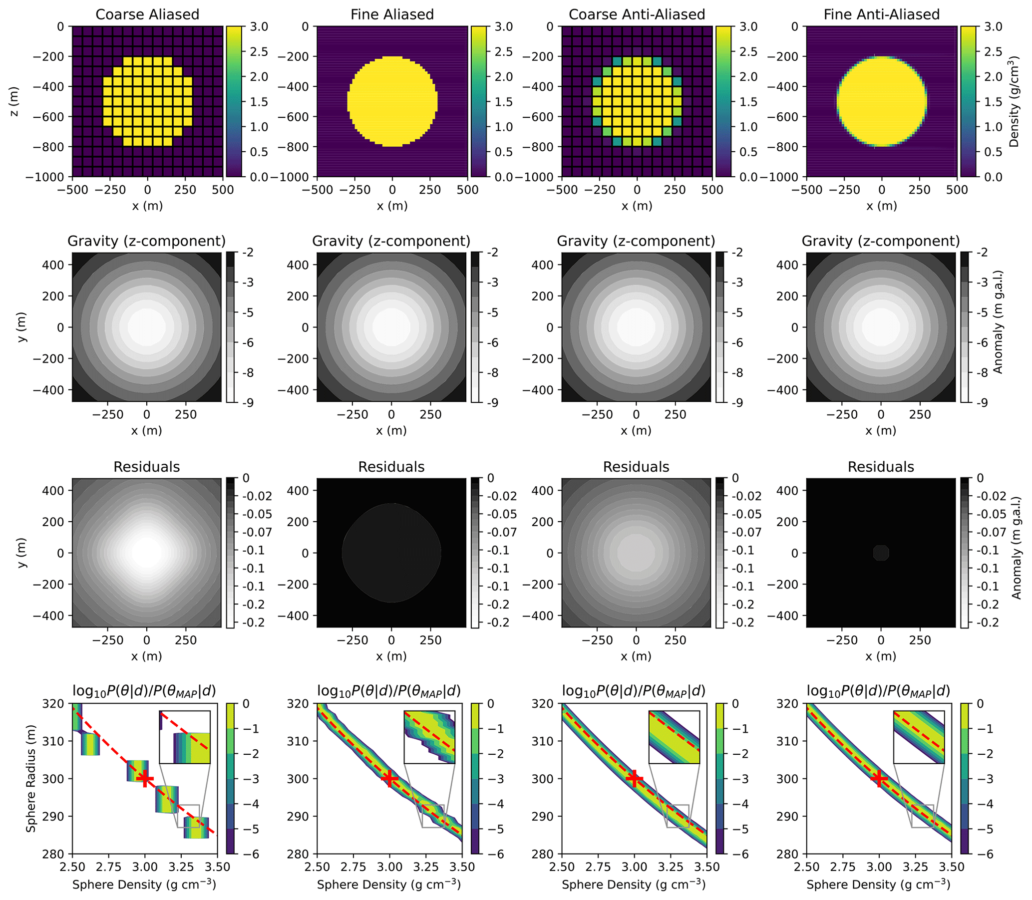
Figure 1Calculation of the posterior distribution for the radius and density of a uniform spherical inclusion from gravity inversion. Top row: cross section of 3-D rock density field for the true model from which the data are generated. Second row: simulated gravity field at the surface. Third row: residuals of simulated gravity field from the analytic solution. Bottom row: cross section through the posterior for an independent Gaussian likelihood. Discretization schemes shown (columns, left to right): coarse aliased mesh (153 cells), fine aliased mesh (603 cells), coarse anti-aliased mesh, fine anti-aliased mesh. The true parameters are shown by the red crosses, while the dashed red lines indicate the degeneracy relation in Eq. (2) that constitutes the maximum-likelihood ridge of the analytic solution.
When inverting on the coarse mesh with no anti-aliasing, the density in a given cell changes only when the sphere radius crosses over the center of one or more mesh cells, and then it changes discontinuously (see last row, first column of Fig. 1). This in turn induces spurious structure into the likelihood, and hence the posterior distribution of the inversion parameters. The numerical posterior becomes a collection of isolated modes scattered along the locus of degeneracy (dashed red line) between ρ (y axis) and R (x axis) on which the true parameters (red cross) lie, none of which appropriately quantify the uncertainty in the true analytic problem. These artifacts can be suppressed by refining the mesh, though at the cost of increasing the number of voxels (and the computation time); in this case, by a factor of 43=64. Importantly, the underlying posterior for this high-resolution mesh is not free of discontinuities, but takes on a terraced appearance.
The inversions with anti-aliased geology result in continuous, even smooth, posteriors that trace the analytic solution and run at nearly the same speed. A closer look reveals that the coarse-mesh anti-aliased posterior is slightly offset toward the bottom left relative to the analytic curve, while the fine-mesh posterior is not. This is a product of low mesh resolution, which the anti-aliasing approximation only partially mitigates (see Sect. 2.4). Each anti-aliased interface is treated locally as a plane surface. For a given gravity signal, spheres with a higher density have a smaller radius and thus higher curvature at the interface; the departure from the true posterior will grow as the sphere radius approaches the voxel size. The bias amounts to ∼1 % of the sphere's mass at the true parameter values, which the data are just sufficient to detect. Thus, while anti-aliasing may incidentally improve the accuracy of geophysical field calculations, its primary benefit is to reproduce the continuous structure of the underlying likelihood.
We will later directly test the influence of aliasing on the performance of MCMC, since the capacity for full posterior inference is one of the major advantages of parametric geological inversions. However, aliasing will cause problems for a broad variety of estimation algorithms. Even for fine mesh resolution, the likelihood is piecewise constant along spatially aliased geological parameters, and so components of the likelihood gradient in those directions are zero almost everywhere in a measure-theoretic sense. Methods such as Nelder–Mead (for optimization) and Metropolis random walk (for sampling) that do not rely on posterior gradient information will seem to work with a fine enough mesh, although at greater computational cost and with no warning of the extent of aliasing effects unless run multiple times from different starting points. Gradient-based methods, such as stochastic gradient descent or Hamiltonian Monte Carlo, will fail catastrophically, since the zero gradient of an aliased likelihood will not reflect its geometry. The covariance matrix used to estimate local uncertainty in the fit from an optimization algorithm will be singular, since the components of the Hessian along aliased directions will be zero. Finally, while the gravity inverse problems we consider in this paper are linear, an attempt to invert for parametric geology based on a nonlinear sensor would face discontinuous changes in the sensitivity kernel with parameters, with unpredictable effects on parameter estimation.
One could argue that the likelihood might be less badly aliased if the data constraints were weaker. Inflating the data errors can be viewed as a form of tempering, which we would expect to merge the multiple aliased modes. Figure 2 shows the results of inflating the errors in the “coarse aliased” discretization of the sphere problem by various factors until the isolated modes in the original problem have merged. The distribution becomes fully navigable only for data errors a factor of 5–10 times larger than our original problem – that is, for data errors comparable to the amplitude of the signal itself. Furthermore, the blockiness or terracing is a function of the discretization scale only, so that any estimation methods relying on gradients will break down along the aliased spatial parameters in the same way as before.
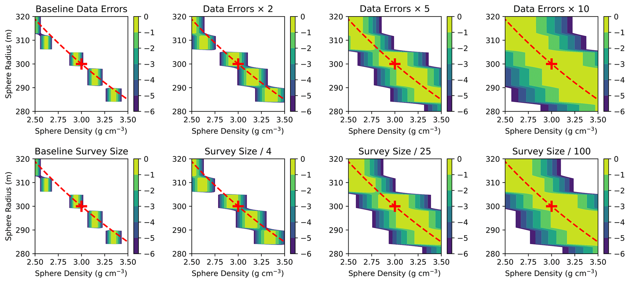
Figure 2Influence of data error on the posterior distribution for the sphere inversion problem. The panels from left to right show the effects of multiplying the standard deviation of Gaussian noise on gravity observations by factors of 1 (baseline), 2, 5, and 10.
This kind of catastrophic breakdown occurs because of the restrictive conditioning of rock properties on parametric geology, so we do not expect the same kind of effect to arise in flexible geophysical inversions that derive their priors from discretized geological models (e.g., Giraud et al., 2021b). The geophysical sensor model is a smooth function of the rock properties, and so, when the rock properties are the primary model parameters, the likelihood remains smooth. Highly restrictive model error terms that are inconsistent with the data may still hamper performance or inference. While it would be interesting to examine nonzero voxelization model errors for the kind of parametric inversion we investigate in this paper, this is a technically complex issue that we defer to future work. For now we note simply that aliasing still arises even in a parametric model that is in other respects perfectly specified, and that treating it explicitly will remove aliasing contributions to model errors in future parametric inversions.
While our example may seem artificial, widely used geological modeling tools such as Noddy and GeoModeller usually export on rectangular meshes, with lithology or rock properties evaluated at the center of each mesh cell precisely as described above. Any ongoing development or support of geological modeling tools intended for use in probabilistic workflows should keep examples like this in mind. Complex structure imparted by faults, folding, dykes, and sills is highly sensitive to discretization. The situation may arise where the causative body for a strong geophysical anomaly, such as a thin and relatively magnetic or remanently magnetized dyke, is removed from the geological prior due to overly coarse discretization parameters, while a resulting strong magnetic response remains. Inversion schemes are not intended to address situations where the target is unintentionally removed from the data.
2.3 Fitting an anti-aliasing function
The main idea behind anti-aliasing is to produce rock property values in each mesh cell such that the response of a sensor to the anti-aliased model best approximates the action of the same sensor on the same geology exported to a higher-resolution mesh. In this section, we will develop an anti-aliasing prescription for gravity anomaly, which responds linearly to mass density. We frame the problem as a regression that uses the position of a geological interface within a mesh cell to predict what the mean mass density would be for that cell in a high-resolution model.
The top panel of Fig. 3 shows the geometry of the problem. For simplicity, we assume constant rock density within each unit, which reduces the problem to predicting the fraction of the cell's volume lying to either side of the interface. We further assume that the interface is flat at the spatial scale of a single mesh cell, so that it can be approximated by a plane surface defined by a point and a unit normal . Due to the translational symmetry of a plane, the influence of r can be reduced to the projected distance u⟂ of the plane from the voxel center r0. The unit normal n can be described in terms of two angles in spherical coordinates; due to the rotational symmetries of a cubical voxel, it is enough to specify the polar angle with respect to the normal to the cube face that a ray drawn from r0 along n intersects, and the azimuthal angle with respect to a coordinate system projected onto that cube face. Expressing the angles in terms of ratios of components of n results in three main predictive features:
where h is the voxel size, , , and r0 is the voxel center.
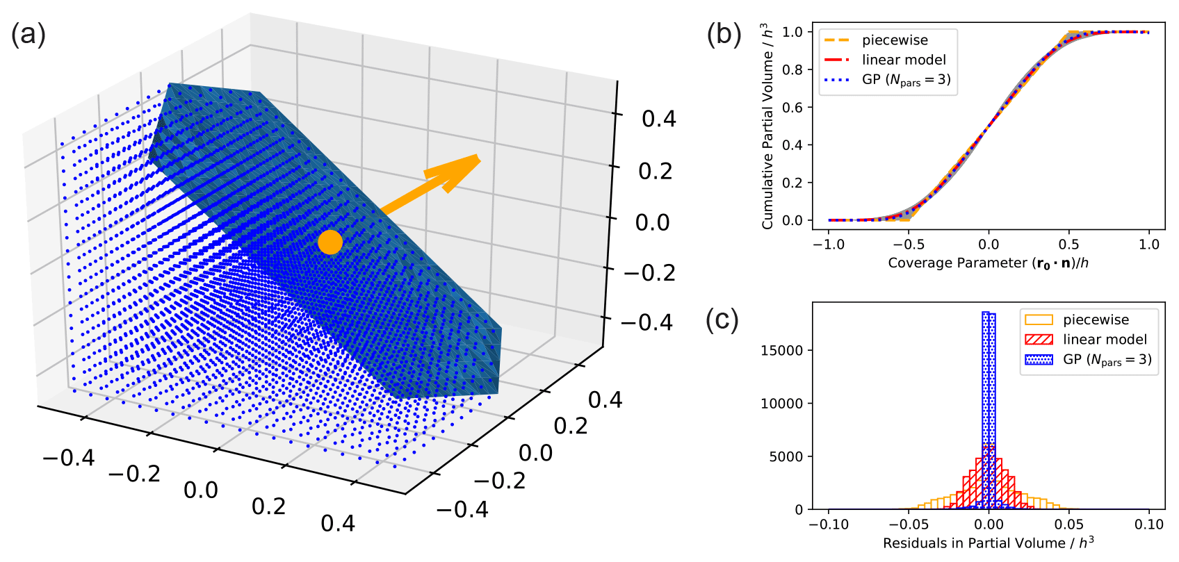
Figure 3(a) Numerical approach to calculating partial volumes. The interface is approximated by a plane running through the voxel. A cloud of points is generated in a regular grid, and the partial volume is then the fraction of these points that satisfy , where is a point on the interface and is a unit normal vector. (b) Regression models for fast evaluation of partial volumes using data generated from the approximate numerical scheme (gray curves): a piecewise linear interpolation over u⟂ (red), a generalized linear model with up to third-order terms (blue), and a Gaussian process that also includes features associated with the orientation of the interface (green). (c) Precision of partial volume models. The piecewise model reaches 2 % RMS accuracy. A linear regression reaches 1 % accuracy, as does a Gaussian process regression with a single feature u⟂. A GP with three features that captures the directionality of the interface with respect to the cube boundaries reaches 0.3 % accuracy.
To train the regression, we generate a synthetic dataset of 1000 (r,n) pairs with which a plane interface might intersect a generic voxel. In each pair, r is distributed uniformly in space, and n uniformly in solid angle. We calculate the partial voxel volume beneath the plane numerically by mesh refinement to 20× higher resolution.
Figure 3 shows three different possible functional forms for the regression: a piecewise linear function of u⟂ alone; a linear regression model including interaction terms up to third order, where the regressors have been transformed by a hyperbolic tangent function to maintain boundary conditions and keep fractional volumes between 0 and 1; and a Gaussian process regression. A linear regression model based on the single feature u⟂ – the normal distance to the plane from the voxel center – can provide smooth anti-aliasing to 1 % RMS accuracy (5 % worst-case); the optimized form is
This functional form provides negligible computational overhead in our implementation as part of a MCMC inversion loop and has derivatives of all orders. Including orientation features in the linear regression results in negligible improvements in accuracy while increasing computation time. The Gaussian process does not provide meaningful improvement over the linear regression using u⟂ alone; it attains an accuracy of 0.3 % RMS (3 % in the worst case) using three features, but is many times slower to evaluate. We use Eq. (6) for further experiments in this paper.
2.4 Potential limitations of anti-aliasing
Since the anti-aliasing approximation amounts to a strong prior on sub-mesh structure, understanding its limitations is critical in practical modeling. The approximation giving rise to Eqs. (3) and (6) will break down when interface curvature becomes significant. Common sense suggests that no length scale parameter in the inference problem should ever be less than the voxel size h. These situations can be difficult to detect from inside the inversion. Spatial scale parameters, such as fold wavelengths, may produce high-curvature interfaces only in some regions of parameter space. Curvature measured using the Hessian adds computational overhead and may miss structures beneath the Nyquist limit if evaluated on the same mesh as the inversion itself. However, as shown in Fig. 1, departures from the true posterior can occur even at higher resolution, depending upon the resolving power of the data and the structure of the likelihood.
Another drawback in anti-aliasing is that it ignores the relative orientations of interfaces in voxels spanning multiple interfaces. If only one interface passes through a voxel, Eq. (6) should result in a faithful representation of its density. If, however, that voxel is later faulted or brought up against an unconformity, the true mean density in the voxel depends on which of the two formations is preferentially replaced by the new obtruding unit; Eq. (6) will only give some mean value that is roughly correct when the two interfaces intersect at right angles. Anti-aliasing will thus become increasingly inaccurate with each successive application to a voxel. This effect can cause biases even in geologies with exactly flat interfaces; we expect it to be more pronounced in models with multiply faulted interfaces in regions where the geophysical sensitivity is the highest, for example, near the surface. Such regions of complexity can be identified by flagging voxels within a projected distance of an interface, and the additional uncertainty in the lithology can be treated explicitly – for example, by assigning latent variables in the statistical model to account for it.
Once an inversion has been performed, the best practice to assess bias will still be to repeat it with a different cell size. In the next section we will discuss metrics to evaluate the global agreement of posteriors based on different mesh sizes, allowing quantitative evaluation, online or offline, of the value to the user of running at a given mesh resolution.
To illustrate how anti-aliasing interacts with more realistic geological structures, Blockworlds implements a simplified kinematic model inspired by Noddy (Jessell, 1981; Jessell and Valenta, 1993). We chose to write our own demonstration code rather than modifying Noddy both for ease of prototyping and to demonstrate how anti-aliasing interacts with the kinematic calculations. We construct a range of 3-D models and visualize slices through each Bayesian model posterior to demonstrate the influence of anti-aliasing on the calculations.
3.1 Kinematic model events
The action of kinematic events in Blockworlds is recursive, with each new event modifying the geology resulting from the events before it. Since the notation describing this action is complex, we include a summary of symbols defined in this subsection in Table 1.
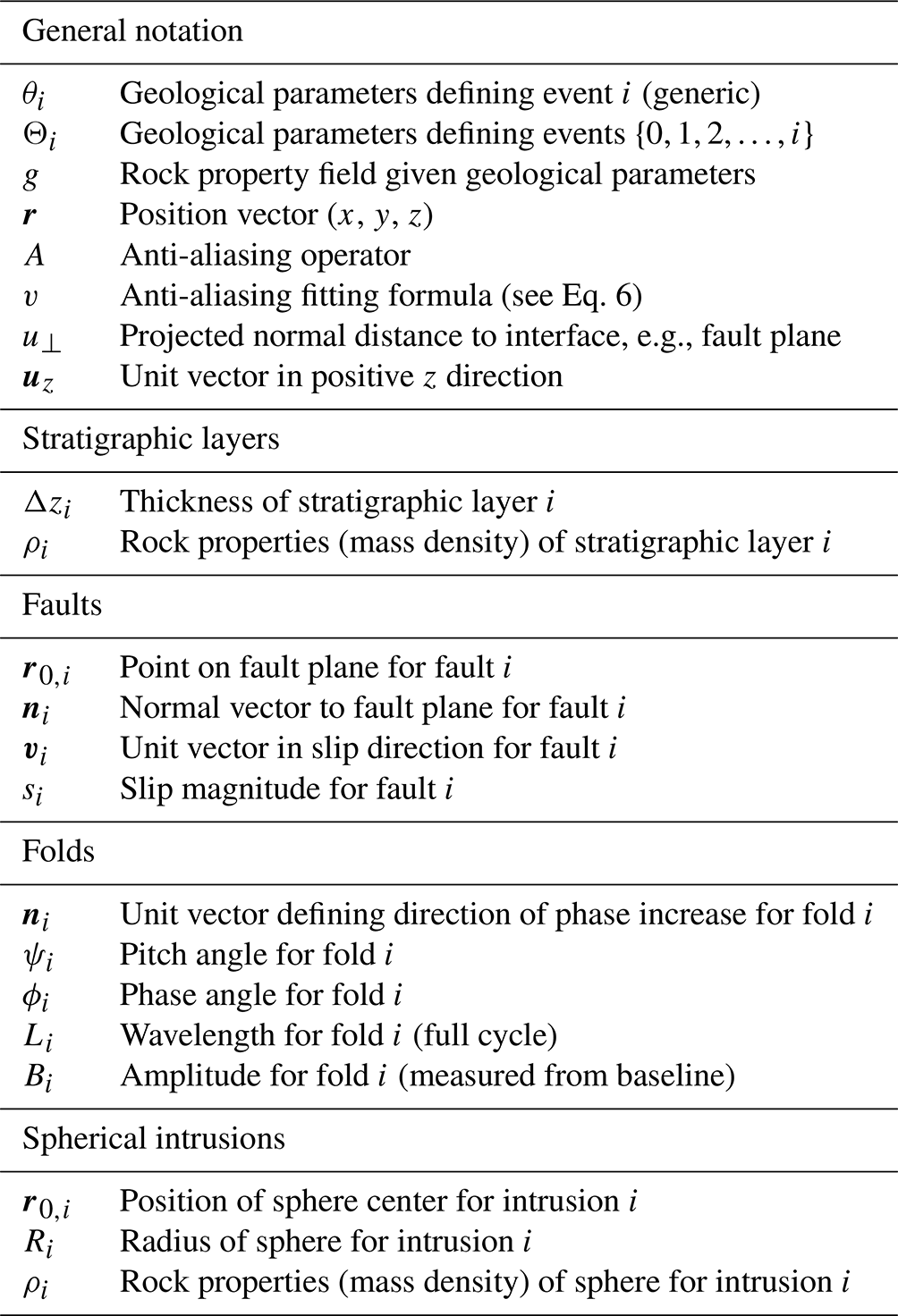
Each event is parametrized by a collection of parameters θi, with denoting the collection of parameters for all events up to event i. We denote the function that renders 3-D rock properties based on all events up to event i by gi(r|Θi). Although geology can be evaluated on a mesh of any desired resolution, in practice the recursive evaluation means that each event modifies rock properties as rendered on the same discrete mesh as the previous event.
The calculation begins with a basement layer of uniform density, , which has no interfaces and thus requires no anti-aliasing. The action of the anti-aliasing operator A for an interface between two sub-volumes with spatial rock property fields g+ and g− at a projected distance u⟂ from the voxel center is given by
where u⟂ and v(u⟂) are given by Eqs. (3) and (6). The anti-aliasing must be applied in the co-moving coordinate frame of each event, so that rock properties stored on the discrete rock property mesh are recursively averaged or transported by later events (see Fig. 4). Note also that u⟂, and thus A, depends on the mesh spacing.

Figure 4Calculation of forward geology for Models 1 and 8 through a sequence of tectonic events: the addition of two stratigraphic layers and two faults. Top: geology; bottom: anti-aliased, voxelized rendering.
The Blockworlds code covers four elementary event types, each parametrized by its own scalar field that takes a zero value at the relevant interface:
-
Stratigraphic layer. for a layer with thickness Δzi and mass density ρi, which has the effect of laying a new layer down on top of the existing geology:
-
Fault. for a fault passing through a point r0,i with unit normal ni and dip-slip displacement si. Our parametrization constrains to lie on the surface, and uses a polar representation for n derived from dip and dip direction (Pakyuz-Charrier et al., 2018b). Given these elements, we calculate , resulting in a unit vector pointing in the dip-slip direction parallel to the fault plane, with no strike-slip component. Then
which has the effect of displacing the geology in the half-space by the slip vector sv.
-
Fold. for a fold defined by a unit vector ni, pitch angle ψi, phase angle ϕi, wavelength Li and amplitude Bi. Given ni, we generate two unit vectors and , defining an orthonormal structural frame . Rock elements are displaced laterally by a vector field
so that the rock properties after the fold are given by
-
Spherical intrusion. for a sphere of radius Ri and uniform density ρi centered at r0,i:
Figure 4 shows the action of the kinematic elements of the model alongside an anti-aliased version of the voxelized density volume, calculated over a 1 km3 rectilinear mesh voxels on a side.
3.2 Setup of specific 3-D models
We construct a series of 15 kinematic models with true configurations as shown in Fig. 5. Each model occupies a 1 km3 cubical volume, and is discretized on a rectilinear mesh with cubical voxels. All have three stratigraphic layers and two additional tectonic events, varying in order and positioning.
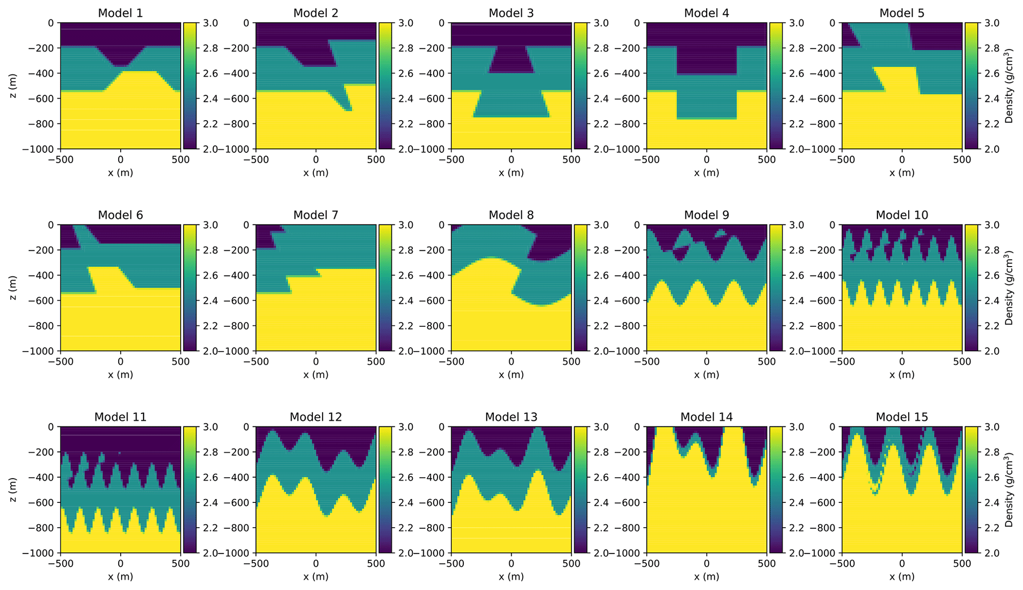
Figure 5Voxelized final states of all models in the suite, displaying 3-D geology in cross section.
The first set of models focus on planar dip-slip faults, with final configurations as follows:
-
Model 1: a typical graben structure with two intersecting faults, both exhibiting normal movement
-
Model 2: a negative flower structure resulting from transtension, where both a sub-vertical fault and high-angle fault exhibit normal movement
-
Model 3: two reverse faults dipping at the same angle and away from each other
-
Model 4: two parallel sub-vertical faults of opposing displacement – the left fault with left-side-up movement, the right fault with right-side-up movement
-
Model 5: a positive flower structure resulting from transpression, where both a sub-vertical fault and high-angle fault exhibit reverse movement
-
Model 6: two high-angle faults, the left displaying thrust movement and the right displaying normal movement
-
Model 7: a similar scenario to Model 6, except the movement for both faults is reversed.
We also include some additional folded configurations, selected to test the anticipated limitations of anti-aliasing described in Sect. 2.4 (these use the same stratigraphic history as the two-fault events except when parameter changes are explicitly noted):
-
Model 8: an upright, open fold of 500 m wavelength, with a west-dipping, high-angle reverse fault offsetting the fold limbs
-
Model 9: a tighter fold of wavelength 300 m, cut across by a low-angle reverse fault to create near-surface voxels in the block model traversed by multiple interfaces
-
Model 10: a more extreme version of Model 9 created by reducing the fold wavelength to 150 m, near the Nyquist sampling limit for the coarse voxel size
-
Model 11: similar to Model 10, but with a deeper surface layer to create aliased voxels farther beneath the surface
-
Model 12: a folded fold, with two folds of wavelength 300 m and with the second upright fold at 70∘ azimuthal with respect to the first
-
Model 13: two upright folds of different wavelengths (300 and 500 m) with axes aligned
-
Model 14: a version of Model 13 with thinner surface stratigraphic layers (75 m each) to create near-surface voxels with multiple parallel interfaces
-
Model 15: a stratigraphy with a thinner surface layer (150 m) and a low-angle reverse fault that has been folded, again to create a final state with high complexity in near-surface voxels.
Table 2Parameter true values and prior distributions for fault-focused kinematic models labeled M1 to M7. The prior mean is set to the true value for each parameter.
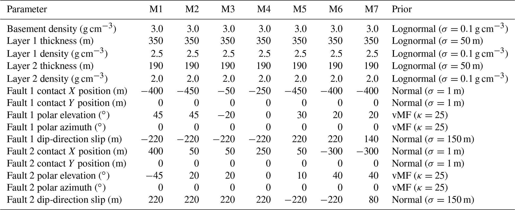
Table 3Parameter true values and prior distributions for fold-focused kinematic models labeled M8 to M15. * In M15, the stratigraphy is faulted first, then folded.
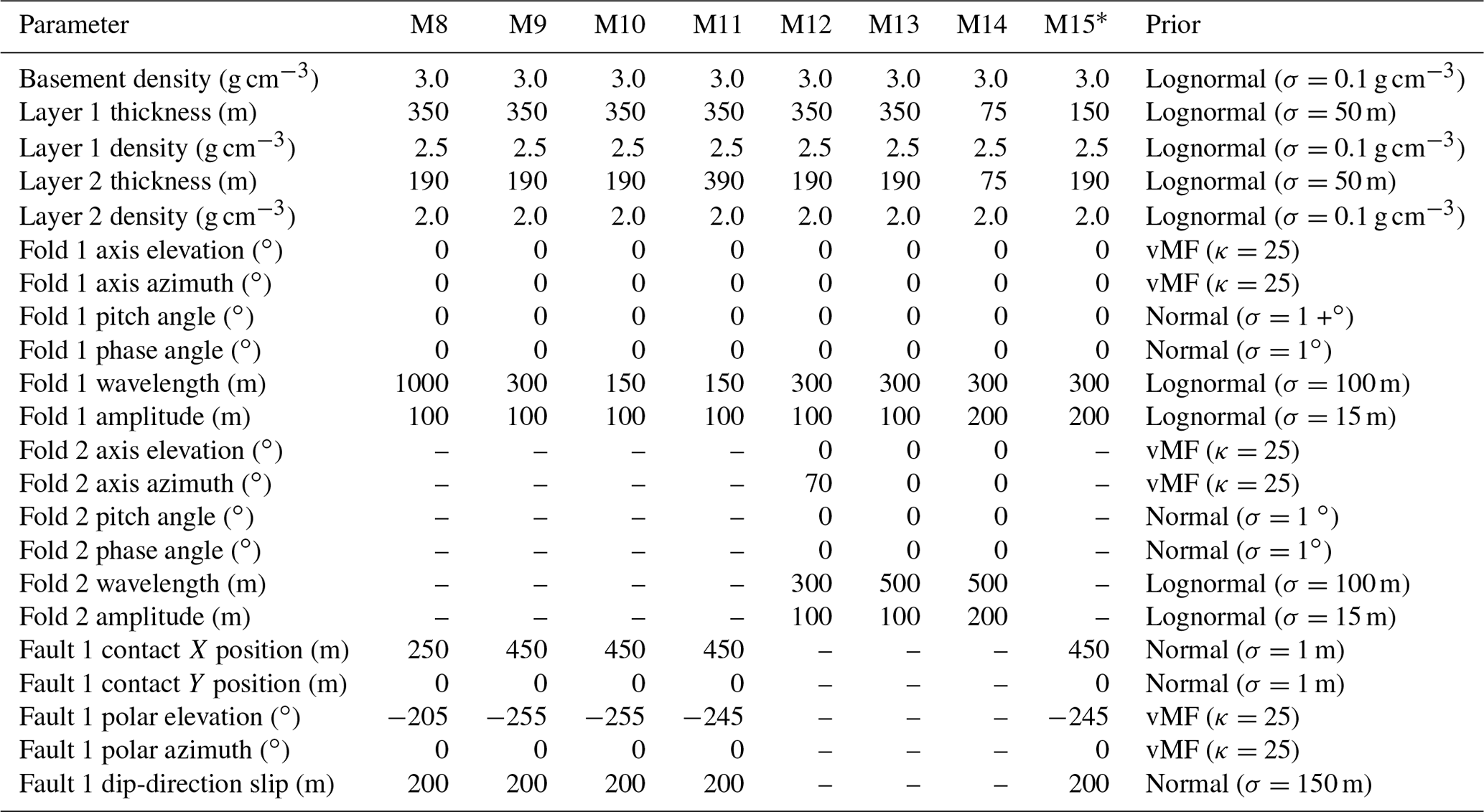
We choose prior distributions for the parameters to simulate the realistic incorporation of structural geological knowledge, as shown in Tables 2 and 3. We use normal and lognormal distributions over non-negative quantities, and von Mises–Fisher distributions over angular quantities, for simplicity and interpretability in terms of scale parameters, which reflect the precision of available structural information. The positions of the anchor points lying on the fault planes have very narrow priors (σ=1 m), appropriate for surface observation localized by GPS. The fault slip parameters reflect rough estimates (σ=150 m), an extent comparable to the true slip value for each fault. The polar representations of the fault directions are constrained by a von Mises–Fisher (vMF) distribution with κ=25, corresponding to a full width at half maximum of about 16∘ (Pakyuz-Charrier et al., 2018b). In each case, the prior mode rests at the true parameter values to ensure that misspecification of the prior does not complicate the aliasing effects we set out to examine.
For each model, we examine four regimes of resolution and aliasing. We consider a “coarse” mesh (h=66.6 m) as well as a “fine” mesh (h=13.3 m), both with and without anti-aliasing. The anti-aliased model on the fine mesh is taken to be the true model for the purposes of calculating a common synthetic forward gravity dataset against which to evaluate the likelihood.
We generate synthetic geophysics data based on the true model parameters, with measurements spaced evenly in a 20×20 grid at the surface (grid spacing of 50 m), and add independent Gaussian noise with a standard deviation σ0 of 5 % of the sample standard deviation of the data across the survey. Each data point yj is thus generated according to
where fj(θ) is the forward model for the geophysical measurement yj given the geological parameters θ. In a realistic situation, we may not know the noise variance σ2 exactly, but we can account for our uncertain knowledge of it by including a hierarchical prior for σ2. If we choose this prior to be an inverse gamma distribution,
the integral over σ2 can be solved analytically, saving the computational expense of sampling over σ2 by MCMC (see McCalman et al., 2014; Scalzo et al., 2019):
so that the likelihood has the form of a t-distribution with ν=2α degrees of freedom and scale parameter . For our experiments, we choose α=2.5, , a weakly informative prior with a mean and mode close to the true variance used to generate the data. The full likelihood is then the product of the likelihoods for independent data points,
As with the earlier synthetic examples for a spherical intrusion, we used SimPEG (version 0.14.0; Cockett et al., 2015; Heagy et al., 2020) for the calculation of forward gravity. The SimPEG Simulation3DIntegral class uses a closed-form integral expression for the contribution to the gravitational field from a rectangular prism of constant density (Okabe, 1979; Li and Oldenburg, 1998): for example, for the z-component,
where is the location of the gravity sensor, runs over each corner of the prism, and with . This form is widely used in geophysics and is one of the benefits of working over rectangular meshes. The total gravity signal is then the sum of the contributions for each mesh cell. Since the expression is linear in the density for each mesh cell, the forward model sensitivities can be cached for fast likelihood evaluation.
3.3 Posterior slices and MCMC sampling
To illustrate some of the effects caused by aliasing and some of the limits of anti-aliasing, we visualize a series of two-dimensional slices through the posterior distribution. Pairs of free parameters are scanned on a regular 30×30 grid centered on their true values, with all other parameters held fixed at their true values. This produces a set of figures similar to Fig. 1 for the kinematic models.
We also perform MCMC over the parameters of the kinematic models to demonstrate the impact of anti-aliasing on chain mixing. The aliased posterior has no useful derivative information for structural parameters, so we are limited to random walk proposals. For our tests, we choose the adaptive Metropolis random walk algorithm of Haario et al. (2001), which is used in contemporary studies such as Wellmann et al. (2017) and is the simplest algorithm likely to give good performance on posteriors with the kind of strong covariances seen in the conditional posterior slices. This algorithm starts from an initial guess θ0 and proposes a new value θ′ at time step t from a multivariate normal distribution centered on the current state θt:
where ηd is a global step size parameter that only depends on the dimension of the space, and
The covariance matrix of the proposal is estimated from the current chain history, so that after an initial nonadaptive random walk period of length t0 steps, the walk gradually transitions from an initial-guess covariance Σ0 to match the estimated posterior covariance. States are accepted according to the usual Metropolis–Hastings criterion, setting with probability
and with probability 1−α. We use an adaptation length of t0=1000 and an initial diagonal covariance matrix of step sizes set to 20 % of the prior width for each parameter (0.02 g cm−3 for densities, 10 m for layer thicknesses, 30 m for fault slips, and 3∘ for angular variables).
We use the coarse mesh for calculations since this will give much faster results for MCMC and highlight the impact of aliasing on chain mixing. We run M=4 chains for N=105 samples from the posterior of each model, with and without anti-aliasing. We initialize each chain with an independent prior draw and discard the first 20 % of samples as burn-in. Each chain took 6 min to run on an Intel Core i7 2.6 GHz processor.
We use the integrated autocorrelation time to measure MCMC efficiency within each chain, and the potential scale reduction factor (PSRF; Gelman and Rubin, 1992) to estimate the extent of convergence to the true posterior. The autocorrelation time τ is the approximate number of chain iterates required to produce a single independent sample from the posterior, so that the chain length N divided by τ becomes one possible measure of effective sample size. The potential scale reduction factor , formed from multiple chains, is the factor by which the posterior variance estimated from those chains could be further reduced by continuing to sample. A PSRF near 1 suggests that multiple chains from different starting conditions have achieved similar means and variances and thus are sampling from a common stationary distribution; a large PSRF shows a residual dependence on starting conditions. The PSRF is usually given for each parameter in a multi-dimensional chain; some dimensions may mix quickly, while others take a long time to converge.
Finally, to quantify the overall accuracy of the posterior density calculation, we use the Kullback–Liebler divergence
where represents the posterior based on a low-resolution mesh (with or without anti-aliasing), and represents the high-resolution, anti-aliased posterior. DKL is a global measure sensitive to biases and covariances across all parameters. Since it requires integration over the posterior, this metric is not available to check results of single-point optimization algorithms. We use the MCMC chain itself to calculate the integral, representing it as the difference in log probability density averaged over samples from the low-resolution posterior.
4.1 Posterior cross sections
Two-dimensional slices through the posterior distribution for selected variable pairs are shown for Model 1 (in Fig. 6) and Model 6 (in Fig. 7). Although we do not include similar figures for every model in the main text, equivalent sets of plots for all models can be regenerated automatically by scripts in the Blockworlds repository.
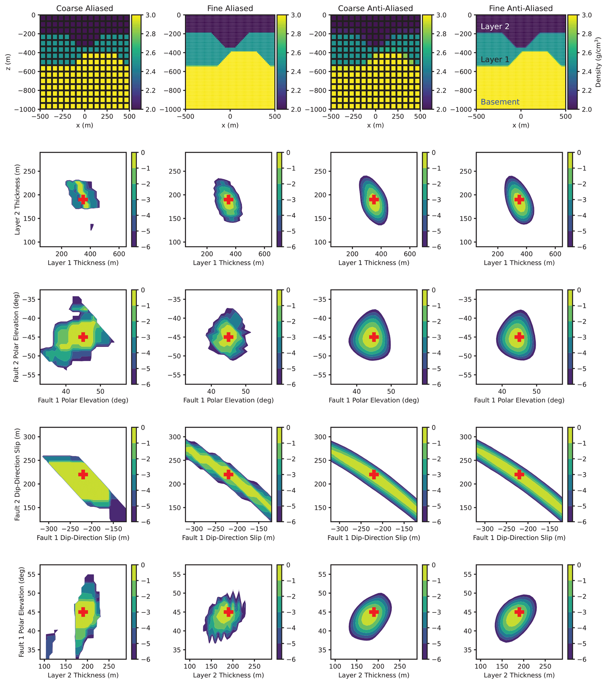
Figure 6The log posterior distribution of pairs of parameters, denoted by θ, in kinematic Model 1, relative to the maximal value , where . In each slice, the true values of gridded parameters are marked with red crosses, and parameters that are not plotted are fixed at their true values. Columns correspond to different discretization schemes; from left to right: coarse mesh (153) with no anti-aliasing; fine mesh (753) with no anti-aliasing; coarse mesh with anti-aliasing; fine mesh with anti-aliasing. The top row shows a vertical cross section at y=0 of the 3-D rock density field under each discretization scheme. Rows 2–5 correspond to different pairs of parameters in θ; for row 2, θ consists of the two non-basement layer thicknesses; for row 3, θ consists of the dip direction angles of the two faults; for row 4, θ consists of the fault slips; for row 5, θ consists of the dip of the first fault and the thickness of the top layer.
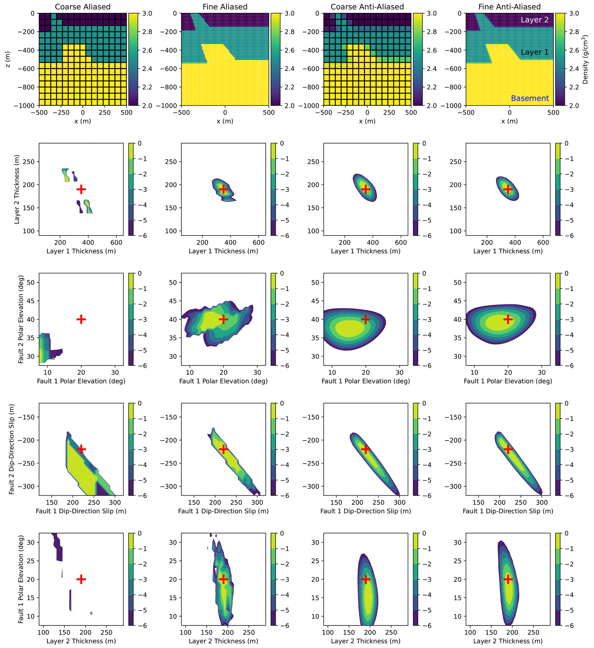
Figure 7The log posterior distribution of pairs of parameters for Model 6. All plot properties are the same as in Fig. 6.
Model 1 is relatively well behaved; the aliased posterior has a single dominant mode near the true value. This is a situation in which the aliasing effects function mainly to make the likelihood appear blocky and terraced. Although proposals that require derivatives of the likelihood will fail on this posterior, it can still be navigated by appropriately tuned random walks, or by the discontinuous Hamiltonian Monte Carlo sampler of Nishimura et al. (2020).
Nevertheless, the benefits of anti-aliasing are still clear. Merely increasing the mesh resolution of the coarse aliased model by a factor of 5 (and the computational cost by over 100×) is insufficient to completely suppress aliasing artifacts. The coarse aliased model fails to capture the full extent of the very strong correlation between the dip slips of the two faults, though the fine aliased model does so reasonably well. The posteriors of the two anti-aliased models deviate only negligibly from each other for all parameters.
Model 6 presents a more challenging case where a coarse mesh does not fully resolve structures close to the surface, resulting in bias for the low-resolution models. The layer thicknesses of the coarse aliased model are explicitly multi-modal as the interfaces hover between depths, and the modes for several variables are significantly offset from their true values. These values become sharp modes in a broader parameter space, easily missed by any inappropriately scaled MCMC proposal. The fine aliased model reproduces the overall posterior shapes, with some distortions relative to the fine anti-aliased reference model. The coarse anti-aliased model produces a smooth posterior and recovers the correct overall correlations between parameters, but are somewhat offset from the true values.
The differences between low- and high-resolution models are, predictably, more dramatic for folded models where the priors do not exclude fold wavelengths close to the Nyquist limit for the coarse mesh scale, such as Models 10 and 11. Other models, such as Model 9, show that anti-aliasing gives much better results for fold wavelengths greater than the mesh scale. In Model 11, where the undersampled structure is positioned farther beneath the surface, the apparent effects are less apparent than in Model 10, but still appear in directly linked variables such as the fold wavelength.
The biases caused by aliasing seem to be strongest in angular variables such as fault directions. For Model 6, the best-fit dip-slip angles are offset from the true values by more than 10∘, corresponding to the extent through which the scan must sweep to obtain any difference in rock property for a few near-surface voxels in the coarse aliased model. Anti-aliasing the coarse-mesh model largely, but not completely, mitigates this bias. In Model 10, the layer thicknesses are the only model parameters that can be robustly estimated without refining the mesh to resolve structure.
These results confirm that our algorithm can reproduce the continuous behavior in an underlying posterior distribution, and can enable significant computational savings even for complex models as long as the interfaces are smooth on the mesh scale. It cannot – and is not intended to – recover more complex structures beneath the mesh scale that violate the core assumptions under which it was derived.
4.2 MCMC sampling
Table 4 shows the average, best-case, and worst-case values of τ and across all model parameters, as well as the K–L divergence DKL. The posterior is challenging to navigate and all chains have autocorrelation times of the order of hundreds to thousands of samples, comparable to the performance of Obsidian for the Moomba models (Scalzo et al., 2019). Chains for anti-aliased models have autocorrelation times that are shorter by a factor of 2–10 than chains for aliased models, owing to the smoother, more Gaussian structure of the posterior. Most dramatically, the aliased chains still have large PSRF for several variables, even after 105 samples. The anti-aliased chains converge more consistently to the same distribution, with final PSRF values close to 1 for all variables for most models, and much closer to 1 than the aliased chains even for the more challenging, adversarial model configurations.
Table 4Performance metrics for each MCMC run: mean (best-case, worst-case) integrated autocorrelation time τ in samples (×103); mean (best-case, worst-case) potential scale reduction factor calculated across four runs starting from independent prior draws; and sample Kullback–Liebler divergence DKL between the given model and the fine-mesh anti-aliased version, calculated by combining samples from all four runs thinned by a factor of 1000. Runs marked with “AA” are coarse-mesh anti-aliased, while those marked with only a single-digit model number have anti-aliasing turned off.
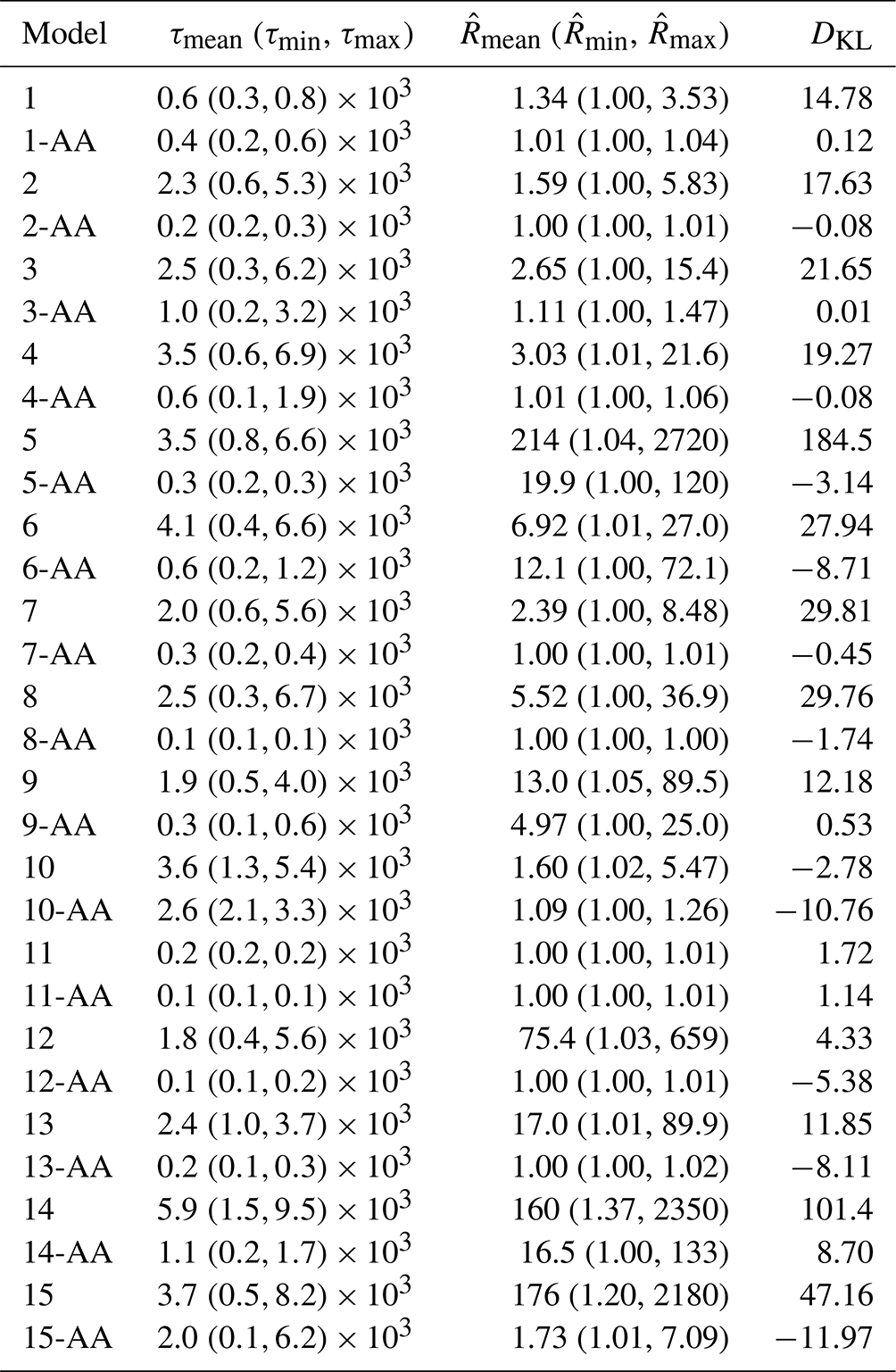
Models 5, 6, 10, 14, and 15 are challenging models for which the anti-aliased chain also has trouble mixing fully. An example trace plot from Model 5 is shown in Fig. 8. One of the chains in the anti-aliased version has fallen into a different mode from the other three, characterized by shifts in the thicknesses and densities of stratigraphic layers as well as a shift in the dip angle of the fault. In contrast, none of the four traces in the aliased model seems to be sampling from the same distribution; each chain has learned a different proposal scaling, and chains occasionally jump between modes at adjacent parameter values characteristic of the ones seen in lower-dimensional projections. Each chain, considered on its own, would give a very different impression of the uncertainty in the inversion. This qualitative behavior is characteristic of sampling for the other models.

Figure 8Trace plots for Fault 1 basement density during MCMC sampling of Model 5 (coarse mesh). The four colors in each plot represent four separate chains started from different prior draws. Traces begin at the end of burn-in and are thinned by a factor of 100 (every 100th trace point is shown). (a) Aliased model. (b) Anti-aliased model.
Complementing the trace plots and MCMC performance metrics as a global measure of posterior inference accuracy, the K–L divergence shows that anti-aliasing usually improves correspondence with the reference posterior (the high-resolution, anti-aliased posterior) by a large margin. Anti-aliased models with large values of DKL correspond well with sub-Nyquist structures or with regions of complexity close to the surface, confirming our intuition that inference in these models benefits from a finer mesh resolution. The aliased posteriors show differences from the high-resolution posteriors spanning many orders of magnitude in probability density, averaged over those modes the chain was able to reach. Since the aliased chains did not in general mix well, their values of DKL should be taken as indicative, whereas the anti-aliased chains with low represent more robust estimates of the true divergence.
To fully characterize uncertainty in truly multi-modal problems, parallel tempering should be used to sample from all modes in proportion to their posterior probability. However, without anti-aliasing, the low-temperature chain in the tempering scheme will mix poorly and will rely more heavily on swap proposals to explore the posterior. The modes that do appear in anti-aliased posteriors are also more likely to represent distinct interpretations, rather than poorly resolved strong correlations between variables.
We have experimentally demonstrated the use and benefit of anti-aliasing only for kinematic models acting on a regular rectangular mesh. However, we see several natural extensions to this work that extend the range and impact of anti-aliasing for parametric geological models. We describe these future directions in the following section.
5.1 Anti-aliasing in terms of the implicit scalar field
Although Blockworlds forward models geology through the action of parametrized tectonic events, it is still an implicit model in the sense that the unit interfaces are defined to be level sets of a scalar field, which we parametrize simply in terms of the distance to the interface. The mathematics of our anti-aliasing prescription generalizes to any differentiable scalar field, including those used in co-kriging models that interpolate structural measurements (Lajaunie et al., 1997; Calcagno et al., 2008). These models will have different posterior geometries than kinematic models, since the modification of structural parameters produces more localized changes in the block models. However, we see no intrinsic reason why the following treatment for general scalar fields should not work just as well as for other types of implicit models, provided the interpolated geological structures have minimal curvature on the mesh scale.
For implicit geological models, each interface is defined as the level set Φ(r)=Φ0 of some scalar field Φ. The value of Φ corresponds roughly to depth or to geological time, but has no intrinsic physical meaning except to ensure that the geologic series of interfaces it defines are conformable. In interpolation models, the specific value Φ0 representing an interface is fixed by observations (from surface measurements or boreholes). In this case, u⟂ can be calculated easily by locally calibrating the scalar field to represent a physical distance in the neighborhood of an interface: for a voxel centered at r0, a first-order approximation of Φ gives
which, using Eq. (3) and writing the interface unit normal as , can be rearranged to give
In this way, each voxel can be anti-aliased simply by evaluating the scalar field and its gradient at the voxel center. For co-kriging models, the scalar field itself must be evaluated at the voxel centers to render it, and the field gradient can be evaluated straightforwardly using the same trained model by differentiating the kernel.
5.2 Anti-aliasing in curvilinear coordinates
The development of the anti-aliasing mapping in Sect. 2.3 and its generalization in Sect. 5.1 assume that each voxel is a cube. However, mesh cells with varying aspect ratios are common in geophysical inversions, for example in dealing with varying sensitivity with depth or with boundary conditions where high resolution is less important. It may also be useful for some problems to work in curvilinear coordinates.
Another useful avenue of future work would be to extend Eq. (23) to more general coordinate systems. Let be the Jacobian of the transformation from dimensionless coordinates u on a unit voxel to physical coordinates r, so that to first order . Equation (3), defining the projection of a reference point in the voxel onto an interface running through the voxel, then becomes
and Eq. (3), defining u⟂ in terms of scalar field values for an implicit model, becomes
5.3 Anti-aliasing for other geophysical sensors
In this paper we have focused on gravity, since it is among the most widely used geophysical sensors in an exploration context and its linear response makes an anti-aliasing treatment straightforward. All of our results extend immediately to magnetic sensors given the strong mathematical equivalence, and may also be appropriate for linear forward models of other sensors such as thermal or electric conductivity, or for the slowness in travel-time tomography.
Useful schemes to anti-alias forward-modeled geology may exist for other sensors, as long as the sensor action at scales smaller than the mesh spacing can be usefully approximated by a computationally simple function of the rock properties and the interface geometry. Frequency-dependent sensors that probe a range of physical scales may require a frequency-dependent anti-aliasing function, and similarly for sensors with anisotropic interactions with interfaces. While there is nothing fundamental that prevents anti-aliasing for sensors that respond nonlinearly to rock properties, mesh refinement may be more important in these cases to ensure the numerical accuracy, as well as the continuity, of the posterior. The framework in this paper treats only quantities defined at mesh cell centers; while it may be possible to derive similar relations for quantities defined on mesh cell faces and edges, as in finite-volume treatments of electromagnetic sensors, this represents future work.
Our experiments show the potential pitfalls of using oversimplified projections of 3-D structural geology onto a volumetric basis for calculation of synthetic geophysics, and demonstrate an intuitive, efficient solution. Anti-aliasing reproduces the smooth behavior of the underlying posterior with respect to the geological parameters to enhance the convergence of optimization or the mixing of sampling methods and to enable the use of derivative information in these methods. Anti-aliasing enables a fixed volumetric basis to more faithfully represent sensor response to latent discrete geology with interfaces that are flat at the scale of a mesh cell, reducing the computational burden of forward geophysics in an inversion loop. Our algorithm is also coordinate invariant and can be combined with curvilinear meshes, and with mesh refinement techniques such as octrees (e.g., Haber and Heldmann, 2007), for even stronger results. Finally, the K–L divergence between versions of the log posterior using different mesh resolutions can be calculated using MCMC samples either online or in post-processing as a diagnostic, allowing the user to determine how much the problem would benefit from additional mesh refinement.
We have focused on calculations over 3-D Cartesian volumetric meshes because implicit and kinematic models are naturally volumetric, and because existing geological modeling codes already export rock properties onto meshes as block models. Introducing anti-aliasing into these geological models is a minimally invasive modification to enhance their use in MCMC-based Bayesian inversions. Other discretization schemes built to align with geological interfaces, such as pillar grids (Wellmann and Caumon, 2018), may mitigate aliasing along the pillar, but still suffer aliasing of features cutting across the pillar axis and are more limited in their representational power. Alternate methods for calculating gravity and magnetics, such as the Cauchy surface method (Zhdanov and Liu, 2013; Cai and Zhdanov, 2015) or finite-volume methods on tetrahedral meshes (Götze and Lahmeyer, 1988; Schmidt et al., 2020), require many fewer discrete elements than a 3-D volumetric mesh to achieve a given accuracy, since they follow an explicit lower-dimensional discretization of each interface. These methods are most suitable for geological models that already parametrize unit interfaces explicitly. Using them with implicit models, or with kinematic models that work by deforming and transporting volumetric elements, would introduce additional computational overhead in tracking the positions of interfaces and updating an associated lower-dimensional mesh. The sensor response coefficients would then also have to be updated each time the model parameters are updated. There may still be geological use cases where tracking interfaces during the sampling process is more efficient than a finite volume solution involving every voxel, but we defer the examination of such cases to future work.
The accurate and efficient projection of these simple geological models onto meshes for geophysics calculations is a prerequisite to inversion for structural and kinematic parameters in more realistic situations. We can now take clear next steps towards MCMC sampling of kinematic histories for richer, higher-dimensional models. In addition, we can now move towards the sampling of hierarchical geophysical inversions that use a parametric structural model as a mean function. This will enable voxel-space inversions for which the geological prior is expressed in terms of uncertain interpretable parameters, or inversions for geology that include uncertainty due to residual rock property variations constrained by geophysics. These would represent more complete probabilistic treatments of geological uncertainty in light of available constraints from geophysics.
In the definitions to follow, we follow notation introduced in Scalzo et al. (2019). Consider M Markov chains, each of length N and with d-dimensional parameter vectors, which are run independently or in parallel. Let denote parameter k of d, drawn at iteration [j] of N in chain i of M. Let
denote the sample mean of parameter k over the N iterates of chain i, and
denote the sample variance of parameter k over chain i. Let denote the sample mean of across all chains. To summarize the variation in parameter estimates across chains, let
denote the sample variance in across chains, and
denote the sample mean of across chains. Thus, Bk is a measure of the variance in parameter estimates made from the history of samples in any single chain on its own, and Wk is a measure of the overall variance of a parameter within any single chain.
A1 Integrated autocorrelation time
The autocorrelation function, measuring the correlation between parameter draws separated by a lag l when treating each chain as a time series, is
The integrated autocorrelation time (IACT), the sum of the autocorrelation function over lags l, gives an estimate of the number of chain samples required to obtain an independent draw from the stationary distribution:
A2 Potential scale reduction factor
The potential scale reduction factor (PSRF) was introduced as a metric for chain convergence by Gelman and Rubin (1992). It measures the extent to which uncertainty in a parameter could be reduced by continuing to sample beyond the nominal chain length N. A simple version that is often implemented is
The behavior of the metric is driven by the ratio , or the variance in parameter means from different chains as a fraction of the overall marginal variance in that parameter. This can be large because of small number of statistics in a unimodal problem, but it can also be large because of poor mixing between modes in a multimodal problem, which increases the autocorrelation between samples. Gelman and Rubin (1992) advocate searching for multiple modes in advance and drawing starting points for MCMC from an overdispersed approximation to the posterior. They also account for sampling variability, including correlation between samples, via the modified metric
where represents the number of degrees of freedom in a t-distribution for , with
We use the metric for our experiments, given that autocorrelation times can be quite long for our chains.
The version of the Blockworlds model code used in this paper is archived with Zenodo (https://doi.org/10.5281/zenodo.5759225; Scalzo, 2021). The datasets used in the inversions are synthetic and can be reproduced exactly by running a set of scripts from the command line that fix the random number seed used to generate those datasets, as described in the package manual.
The study was conceptualized by SC, who, with MJ, provided funding and resources. RS was responsible for project administration, designed the methodology, wrote the Blockworlds code resulting in v0.1, and carried out the main investigation and formal analysis under supervision from SC, EC, and MJ. RS and ML validated and visualized the results. RS wrote the original draft text, with contributions from ML, for which all coauthors provided a review and critical evaluation.
The contact author has declared that neither they nor their co-authors have any competing interests.
Publisher's note: Copernicus Publications remains neutral with regard to jurisdictional claims in published maps and institutional affiliations.
Parts of this research were conducted by the Australian Research Council Industrial Transformation Training Centre in Data Analytics for Resources and the Environment (DARE), through project number IC190100031. The work has been supported by the Mineral Exploration Cooperative Research Centre, whose activities are funded by the Australian Government's Cooperative Research Centre Programme. This is MinEx CRC Document 2021/34. Mark Lindsay acknowledges funding from ARC DECRA DE190100431 and MinEx CRC. We thank Alistair Reid and Malcolm Sambridge for useful discussions.
This research has been supported by the Australian Research Council (grant nos. IC190100031 and DE190100431).
This paper was edited by Lutz Gross and reviewed by Florian Wellmann and two anonymous referees.
Backus, G. and Gilbert, F.: The Resolving Power of Gross Earth Data, Geophys. J. Royal Astron. Soc., 16, 169–205, https://doi.org/10.1111/j.1365-246X.1968.tb00216.x, 1968. a
Backus, G. and Gilbert, F.: Uniqueness in the inversion of inaccurate gross Earth data, Philos. T. Roy. Soc. Lond A, 266, 123–192, https://doi.org/10.1111/j.1365-246X.1968.tb00216.x, 1970. a
Backus, G. E.: Long-wave elastic anisotropy produced by horizontal layering, J. Geophys. Res., 67, 4427–4440, 1962. a
Backus, G. E. and Gilbert, J. F.: Numerical Applications of a Formalism for Geophysical Inverse Problems, Geophys. J. Roy. Astron. Soc., 13, 247–276, https://doi.org/10.1111/j.1365-246X.1967.tb02159.x, 1967. a
Beardsmore, G., Durrant-Whyte, H., and Callaghan, S. O.: A Bayesian inference tool for geophysical joint inversions, ASEG Extended Abstracts 2016.1 (2016), 1–10, https://doi.org/10.1071/ASEG2016ab131, 2016. a, b, c
Bond, C. E.: Uncertainty in structural interpretation: Lessons to be learnt, J. Struct. Geol., 74, 185–200, https://doi.org/10.1016/j.jsg.2015.03.003, 2015. a
Bosch, M.: Lithologic tomography: From plural geophysical data to lithology estimation, J. Geophys. Res.-Solid, 104, 749–766, https://doi.org/10.1029/1998JB900014, 1999. a
Bosch, M.: Inference Networks in Earth Models with Multiple Components and Data, in: Geophysical Monograph Series, edited by: Moorkamp, M., Lelièvre, P. G., Linde, N., and Khan, A., John Wiley & Sons, Inc, Hoboken, NJ, 29–47, https://doi.org/10.1002/9781118929063.ch3, 2016. a
Bosch, M., Guillen, A., and Ledru, P.: Lithologic tomography: an application to geophysical data from the Cadomian belt of northern Brittany, France, Tectonophysics, 331, 197–227, https://doi.org/10.1016/S0040-1951(00)00243-2, 2001. a
Brunetti, C., Bianchi, M., Pirot, G., and Linde, N.: Hydrogeological Model Selection Among Complex Spatial Priors, Water Resour. Res., 55, 6729–6753, https://doi.org/10.1029/2019WR024840, 2019. a
Cai, H. and Zhdanov, M.: Application of Cauchy-type integrals in developing effective methods for depth-to-basement inversion of gravity and gravity gradiometry data, Geophysics, 80, G81–G94, https://doi.org/10.1190/geo2014-0332.1, 2015. a
Calcagno, P., Chilès, J., Courrioux, G., and Guillen, A.: Geological modelling from field data and geological knowledge, Phys. Earth Planet. Inter., 171, 147–157, https://doi.org/10.1016/j.pepi.2008.06.013, 2008. a, b
Capdeville, Y., Guillot, L., and Marigo, J. J.: 1-D non-periodic homogenization for the seismic wave equation. Geophysical Journal International, Geophys. J. Int., 181, 897–910, 2010. a
Catmull, E.: A hidden-surface algorithm with anti-aliasing, in: Proceedings of the 5th Annual Conference on Computer Graphics and Interactive Techniques, Atlanta, Georgia, USA, 6–11, https://doi.org/10.1145/800248.807360, 1978. a
Cockett, R., Kang, S., Heagy, L. J., Pidlisecky, A., and Oldenburg, D. W.: SimPEG: An open source framework for simulation and gradient based parameter estimation in geophysical applications, Comput. Geosci., 85, 142–154, https://doi.org/10.1016/j.cageo.2015.09.015, 2015. a, b
Cook, R. L.: Stochastic sampling in computer graphics, ACM T. Graph., 5, 51–72, 1986. a
Cordua, K. S., Hansen, T. M., and Mosegaard, K.: Monte Carlo full-waveform inversion of crosshole GPR data using multiple-point geostatistical a priori information, Gwophysics, 77, H19–H31, https://doi.org/10.1190/geo2011-0170.1, 2012. a
Crow, F. C.: The aliasing porblem in computer-generated shaded images, Commun. ACM, 20, 799–805, 1977. a
de la Varga, M., Schaaf, A., and Wellmann, F.: GemPy 1.0: open-source stochastic geological modeling and inversion, Geosci. Model Dev., 12, 1–32, https://doi.org/10.5194/gmd-12-1-2019, 2019. a
de Pasquale, G., Linde, N., Doetsch, J., and Holbrook, W. S.: Probabilistic inference of subsurface heterogeneity and interface geometry using geophysical data, Geophys. J. Int., 217, 816–831, https://doi.org/10.1093/gji/ggz055, 2019. a
Frodeman, R.: Geological reasoning: Geology as an interpretive and historical science, Geol. Soc. Am. Bull., 107, 960–0968, https://doi.org/10.1130/0016-7606(1995)107<0960:GRGAAI>2.3.CO;2, 1995. a
Gallardo, L. A. and Meju, M. A.: Structure-coupled multiphysics imaging in geophysical sciences, Rev.f Geophys., 49, RG1003, https://doi.org/10.1029/2010RG000330, 2011. a
Gelman, A. and Rubin, D.: Inference from Iterative Simulation Using Multiple Sequences, Stat. Sci., 7, 457–472, 1992. a, b, c
Giraud, J., Pakyuz-Charrier, E., Jessell, M., Lindsay, M., Martin, R., and Ogarko, V.: Uncertainty reduction through geologically conditioned petrophysical constraints in joint inversion, Geophysics, 82, ID19–ID34, https://doi.org/10.1190/geo2016-0615.1, 2017. a
Giraud, J., Pakyuz-Charrier, E., Ogarko, V., Jessell, M., Lindsay, M., and Martin, R.: Impact of uncertain geology in constrained geophysical inversion, ASEG Extend. Abstr., 2018, 1, https://doi.org/10.1071/ASEG2018abM1_2F, 2018. a
Giraud, J., Lindsay, M., Ogarko, V., Jessell, M., Martin, R., and Pakyuz-Charrier, E.: Integration of geoscientific uncertainty into geophysical inversion by means of local gradient regularization, Solid Earth, 10, 193–210, https://doi.org/10.5194/se-10-193-2019, 2019a. a
Giraud, J., Ogarko, V., Lindsay, M., Pakyuz-Charrier, E., Jessell, M., and Martin, R.: Sensitivity of constrained joint inversions to geological and petrophysical input data uncertainties with posterior geological analysis, Geophys. J. Int., 218, 666–688, https://doi.org/10.1093/gji/ggz152, 2019b. a
Giraud, J., Lindsay, M., and Jessell, M.: Generalization of level-set inversion to an arbitrary number of geologic units in a regularized least-squares framework, Geophysics, 86, R623–R637, https://doi.org/10.1190/geo2020-0263.1, 2021a. a
Giraud, J., Ogarko, V., Martin, R., Jessell, M., and Lindsay, M.: Structural, petrophysical, and geological constraints in potential field inversion using the Tomofast-x v1.0 open-source code, Geosci. Model Dev., 14, 6681–6709, https://doi.org/10.5194/gmd-14-6681-2021, 2021b. a, b
Götze, H. and Lahmeyer, B.: Application of three‐dimensional interactive modeling in gravity and magnetics, Geophysics, 53, 1096–1108, https://doi.org/10.1190/1.1442546, 1988. a
Grose, L., Ailleres, L., Laurent, G., and Jessell, M.: LoopStructural 1.0: time-aware geological modelling, Geosci. Model Dev., 14, 3915–3937, https://doi.org/10.5194/gmd-14-3915-2021, 2021. a
Haario, H., Saksman, E., and Tamminen, J.: An Adaptive Metropolis Algorithm, Bernoulli, 223, ISBN 1350-7265, https://doi.org/10.2307/3318737, 2001. a
Haber, E. and Heldmann, S.: An octree multigrid method for quasi-static Maxwell's equations with highly discontinuous coefficients, J. Comput. Phys., 223, 783–796, https://doi.org/10.1016/j.jcp.2006.10.012, 2007. a
Hastings, W. K.: Monte Carlo sampling methods using Markov chains and their applications, Biometrika, 57, 97–109, https://doi.org/10.1093/biomet/57.1.97, 1970. a
Heagy, L., Kang, S., Fournier, D., Rosenkjaer, G. K., Capriotti, J., Astic, T., Cowan, D. C., Marchant, D., Mitchell, M., Kuttai, J., Werthmüller, D., Caudillo Mata, L. A., Ye, Z.-K., Koch, F., Smithyman, B., Martens, K., Miller, C., Gohlke, C., … and Perez, F.: simpeg/simpeg: Simulation (v0.14.0), Zenodo [code], https://doi.org/10.5281/zenodo.3860973, 2020. a, b
Houlding, S. W.: 3D Geoscience modeling: computer techniques for geological characterization, Springer Verlag, 85–90, ISBN 3-540-58015-8, 1994. a
Jessell, M., Pakyuz-Charrier, E., Lindsay, M., Giraud, J., and de Kemp, E.: Assessing and Mitigating Uncertainty in Three-Dimensional Geologic Models in Contrasting Geologic Scenarios, in: Metals, Minerals, and Society, SEG – Society of Economic Geologists, https://doi.org/10.5382/SP.21.04, 2018. a
Jessell, M. W.: “Noddy” – An interactive Map creation Package, MS thesis, Imperial College of Science and Technology, London, UK, https://tectonique.net/noddy/ (last access: 11 April 2009), 1981. a, b
Jessell, M. W. and Valenta, R. K.: Structural geophysics: Integrated structural and geophysical modelling, in: Structural Geology and Personal Computers, edited by: De Paor, D. G., Elsevier, Oxford, UK, 303–324, https://doi.org/10.1016/S1874-561X(96)80027-7, 1993. a, b
Jessell, M. W., Ailleres, L., and de Kemp, E. A.: Towards an integrated inversion of geoscientific data: What price of geology?, Tectonophysics, 490, 294–306, https://doi.org/10.1016/j.tecto.2010.05.020, 2010. a
Koene, E. F. M., Wittsten, J., and Robertsson, J. O. A.: Finite-difference modeling of 2-D wave propagation in the vicinity of dipping interfaces: a comparison of anti-aliasing and equivalent medium approaches, https://doi.org/10.1093/gji/ggab444, 2021. a
Lajaunie, C., Courrioux, G., and Manuel, L.: Foliation fields and 3D cartography in geology: Principles of a method based on potential interpolation, Math. Geol., 29, 571–584, https://doi.org/10.1007/BF02775087, 1997. a, b
Li, W., Lu, W., Qian, J., and Li, Y.: A multiple level-set method for 3D inversion of magnetic data, Geophysics, 82, J61–J81, https://doi.org/10.1190/GEO2016-0530.1, 2017. a
Li, Y. and Oldenburg, D. W.: 3-D inversion of gravity data, Geophysics, 63, 109–119, https://doi.org/10.1190/1.1444302, 1998. a
Linde, N., Ginsbourger, D., Irving, J., Nobile, F., and Doucet, A.: On uncertainty quantification in hydrogeology and hydrogeophysics, Adv. Water Resour., 110, 166–181, https://doi.org/10.1016/j.advwatres.2017.10.014, 2017. a
Lindsay, M., Jessell, M., Ailleres, L., Perrouty, S., de Kemp, E., and Betts, P.: Geodiversity: Exploration of 3D geological model space, Tectonophysics, 594, 27–37, https://doi.org/10.1016/j.tecto.2013.03.013, 2013. a
Lindsay, M. D., Aillères, L., Jessell, M. W., de Kemp, E. A., and Betts, P. G.: Locating and quantifying geological uncertainty in three-dimensional models: Analysis of the Gippsland Basin, southeastern Australia, Tectonophysics, 546–547, 10–27, https://doi.org/10.1016/j.tecto.2012.04.007, 2012. a
McCalman, L., O'Callaghan, S. T., Reid, A., Shen, D., Carter, S., Krieger, L., Beardsmore, G. R., Bonilla, E. V., and Ramos, F. T.: Distributed Bayesian geophysical inversions, in: Proceedings of the Thirty-Ninth Workshop on Geothermal Reservoir Engineering, Stanford University, Stanford, California, USA, 1–11, 2014. a, b, c
Metropolis, N. and Ulam, S.: The Monte Carlo Method, J. Am. Stat. Assoc., 44, 335–341, 1949. a
Metropolis, N., Rosenbluth, A. W., Rosenbluth, M. N., Teller, A. H., and Teller, E.: Equation of State Calculations by Fast Computing Machines, J. Chem. Phys., 21, 1087–1092, https://doi.org/10.1063/1.1699114, 1953. a
Moczo, P., Kristek, J., Vavrycuk, V., Archuleta, R. J., and Halada, L.: 3d heterogeneous staggered-grid finite-difference modeling of seismic motion with volume harmonic and arithmetic averaging of elastic moduli and densities, Bull. Seismol. Soc. Am., 92, 3042–3066, 2002. a
Mosegaard, K. and Sambridge, M.: Monte Carlo analysis of inverse problems, Inverse Problems, 18, R29–R54, https://doi.org/10.1088/0266-5611/18/3/201, 2002. a, b
Mosegaard, K. and Tarantola, A.: Monte Carlo sampling of solutions to inverse problems, J. Geophys. Res.-Solid, 100, 12431–12447, https://doi.org/10.1029/94JB03097, 1995. a, b
Muir, F., Dellinger, J., Etgen, J., and Nichols, D.: Modeling elastic fields across irregular boundaries, Geophysics, 57, 1189–1193, 1992. a
Nishimura, A., Dunson, D., and Lu, J.: Discontinuous Hamiltonian Monte Carlo for discrete parameters and discontinuous likelihoods, Biometrika, 107, 365–380, https://doi.org/10.1093/biomet/asz083, 2020. a
Ogarko, V., Giraud, J., Martin, R., and Jessell, M.: Disjoint interval bound constraints using the alternating direction method of multipliers for geologically constrained inversion: Application to gravity data, Geophysics, 86, G1–G11, https://doi.org/10.1190/geo2019-0633.1, 2021. a
Okabe, M.: Analytical expressions for gravity anomalies due to homogeneous polyhedral bodies and translations into magnetic anomalies, Geophysics, 44, 730, https://doi.org/10.1190/1.1440973, 1979. a
Olierook, H. K., Scalzo, R., Kohn, D., Chandra, R., Farahbakhsh, E., Clark, C., Reddy, S. M., and Müller, R. D.: Bayesian geological and geophysical data fusion for the construction and uncertainty quantification of 3D geological models, Geosci. Front., 12, 479–493, https://doi.org/10.1016/j.gsf.2020.04.015, 2020. a
Osher, S. and Sethian, J. A.: Fronts propagating with curvature-dependent speed: Algorithms based on Hamilton-Jacobi formulations, J. Comput. Phys., 79, 12–49, https://doi.org/10.1016/0021-9991(88)90002-2, 1988. a
Öztireli, A. C.: A Comprehensive Theory and Variational Framework for Anti-aliasing Sampling Patterns, Comput. Graph. Forum, 39, 133–148, 2020. a
Pakyuz-Charrier, E., Giraud, J., Ogarko, V., Lindsay, M., and Jessell, M.: Drillhole uncertainty propagation for three-dimensional geological modeling using Monte Carlo, Tectonophysics, 747–748, 16–39, https://doi.org/10.1016/j.tecto.2018.09.005, 2018a. a
Pakyuz-Charrier, E., Lindsay, M., Ogarko, V., Giraud, J., and Jessell, M.: Monte Carlo simulation for uncertainty estimation on structural data in implicit 3-D geological modeling, a guide for disturbance distribution selection and parameterization, Solid Earth, 9, 385–402, https://doi.org/10.5194/se-9-385-2018, 2018b. a, b, c
Pakyuz-Charrier, E., Jessell, M., Giraud, J., Lindsay, M., and Ogarko, V.: Topological analysis in Monte Carlo simulation for uncertainty propagation, Solid Earth, 10, 1663–1684, https://doi.org/10.5194/se-10-1663-2019, 2019. a
Patil, A., Huard, D., and Fonnesbeck, C. J.: PyMC: Bayesian stochastic modelling in Python, J. Stat. Softw., 35, 1–81, https://doi.org/10.18637/jss.v035.i04, 2010. a
Perrouty, S., Lindsay, M., Jessell, M., Aillères, L., Martin, R., and Bourassa, Y.: 3D modeling of the Ashanti Belt, southwest Ghana: Evidence for a litho-stratigraphic control on gold occurrences within the Birimian Sefwi Group, Ore Geol. Rev., 63, 252–264, https://doi.org/10.1016/j.oregeorev.2014.05.011, 2014. a
Pirot, G., Renard, P., Huber, E., Straubhaar, J., and Huggenberger, P.: Influence of conceptual model uncertainty on contaminant transport forecasting in braided river aquifers, J. Hydrol., 531, 124–141, https://doi.org/10.1016/j.jhydrol.2015.07.036, 2015. a
Pirot, G., Linde, N., Mariethoz, G., and Bradford, J. H.: Probabilistic inversion with graph cuts: Application to the Boise Hydrogeophysical Research Site, Water Resour. Res., 53, 1231–1250, https://doi.org/10.1002/2016WR019347, 2017. a
Pirot, G., Huber, E., Irving, J., and Linde, N.: Reduction of conceptual model uncertainty using ground-penetrating radar profiles: Field-demonstration for a braided-river aquifer, J. Hydrol., 571, 254–264, https://doi.org/10.1016/j.jhydrol.2019.01.047, 2019a. a
Pirot, G., Krityakierne, T., Ginsbourger, D., and Renard, P.: Contaminant source localization via Bayesian global optimization, Hydrol. Earth Syst. Sci., 23, 351–369, https://doi.org/10.5194/hess-23-351-2019, 2019b. a
Quigley, M. C., Bennetts, L. G., Durance, P., Kuhnert, P. M., Lindsay, M. D., Pembleton, K. G., Roberts, M. E., and White, C. J.: The provision and utility of science and uncertainty to decision-makers: earth science case studies, Environ. Syst. Decis., 39, 307–348, https://doi.org/10.1007/s10669-019-09728-0, 2019. a
Rawlinson, N., Fichtner, A., Sambridge, M., and Young, M. K.: Seismic Tomography and the Assessment of Uncertainty, in: Advances in Geophysics, vol. 55, Elsevier, 1–76, https://doi.org/10.1016/bs.agph.2014.08.001, 2014. a, b, c
Scalzo, R. A.: rscalzo/blockworlds: (v0.1.0-beta.3), Zenodo [code], https://doi.org/10.5281/zenodo.5759225, 2021. a
Sambridge, M., Bodin, T., Gallagher, K., and Tkalcic, H.: Transdimensional inference in the geosciences, Philos. T. Roy. Soc. A, 371, 20110547, https://doi.org/10.1098/rsta.2011.0547, 2012. a, b
Santosa, F.: A level-set approach for inverse problems involving obstacles, ESAIM: Control, Optimisation and Calculus of Variations, 1, 17–33, https://doi.org/10.1051/cocv:1996101, 1996. a
Scalzo, R., Kohn, D., Olierook, H., Houseman, G., Chandra, R., Girolami, M., and Cripps, S.: Efficiency and robustness in Monte Carlo sampling for 3-D geophysical inversions with Obsidian v0.1.2: setting up for success, Geosci. Model Dev., 12, 2941–2960, https://doi.org/10.5194/gmd-12-2941-2019, 2019. a, b, c, d
Schmidt, S., Anikiev, D., Götze, H.-J., Gomez Garcia, A., Gomez Dacal, M. L., Meessen, C., Plonka, C., Rodriguez Piceda, C., Spooner, C., and Scheck-Wenderoth, M.: IGMAS+ – a tool for interdisciplinary 3D potential field modelling of complex geological structures, in: EGU General Assembly 2020, EGU2020-8383, https://doi.org/10.5194/egusphere-egu2020-8383, 2020. a
Tarantola, A. and Valette, B.: Generalized nonlinear inverse problems solved using the least squares criterion, Rev. Geophys., 20, 219–232, https://doi.org/10.1029/RG020i002p00219, 1982. a
Varouchakis, E. A., Yetilmezsoy, K., and Karatzas, G. P.: A decision-making framework for sustainable management of groundwater resources under uncertainty: combination of Bayesian risk approach and statistical tools, Water Policy, 21, 602–622, https://doi.org/10.2166/wp.2019.128, 2019. a
Wang, Z., Yin, Z., Caers, J., and Zuo, R.: A Monte Carlo-based framework for risk-return analysis in mineral prospectivity mapping, Geosci. Front., 11, 2297–2308, https://doi.org/10.1016/j.gsf.2020.02.010, 2020. a
Wellmann, F. and Caumon, G.: 3-D Structural geological models: Concepts, methods, and uncertainties, in: Advances in Geophysics, vol. 59, Elsevier, 1–121, https://doi.org/10.1016/bs.agph.2018.09.001, 2018. a, b, c, d
Wellmann, J. F. and Regenauer-Lieb, K.: Uncertainties have a meaning: Information entropy as a quality measure for 3-D geological models, Tectonophysics, 526–529, 207–216, https://doi.org/10.1016/j.tecto.2011.05.001, 2012. a
Wellmann, J. F., Thiele, S. T., Lindsay, M. D., and Jessell, M. W.: pynoddy 1.0: an experimental platform for automated 3-D kinematic and potential field modelling, Geosci. Model Dev., 9, 1019–1035, https://doi.org/10.5194/gmd-9-1019-2016, 2016. a
Wellmann, J. F., de la Varga, M., Murdie, R. E., Gessner, K., and Jessell, M.: Uncertainty estimation for a geological model of the Sandstone greenstone belt, Western Australia – insights from integrated geological and geophysical inversion in a Bayesian inference framework, Geol. Soc. Lond. Spec. Publ., 453, 41–56, https://doi.org/10.1144/SP453.12, 2017. a, b, c, d
Witter, J. B., Trainor-Guitton, W. J., and Siler, D. L.: Uncertainty and risk evaluation during the exploration stage of geothermal development: A review, Geothermics, 78, 233–242, https://doi.org/10.1016/j.geothermics.2018.12.011, 2019. a
Zhdanov, M. S. and Liu, X.: 3-D Cauchy-type integrals for terrain correction of gravity and gravity gradiometry data, Geophys. J. Int., 194, 249–268, https://doi.org/10.1093/gji/ggt120, 2013. a
Zheglova, P., Lelievre, P. G., and Farquharson, C. G.: Multiple level-set joint inversion of traveltime and gravity data with application to ore delineation: A synthetic study, Geophysics, 83, R13–R30, https://doi.org/10.1190/GEO2016-0675.1, 2018. a