the Creative Commons Attribution 4.0 License.
the Creative Commons Attribution 4.0 License.
 | 25 Mar 2022
SciKit-GStat 1.0: a SciPy-flavored geostatistical variogram estimation toolbox written in Python
Geostatistical methods are widely used in almost all geoscientific disciplines, i.e., for interpolation, rescaling, data assimilation or modeling. At its core, geostatistics aims to detect, quantify, describe, analyze and model spatial covariance of observations. The variogram, a tool to describe this spatial covariance in a formalized way, is at the heart of every such method. Unfortunately, many applications of geostatistics focus on the interpolation method or the result rather than the quality of the estimated variogram. Not least because estimating a variogram is commonly left as a task for computers, and some software implementations do not even show a variogram to the user. This is a miss, because the quality of the variogram largely determines whether the application of geostatistics makes sense at all. Furthermore, the Python programming language was missing a mature, well-established and tested package for variogram estimation a couple of years ago.
Here I present SciKit-GStat, an open-source Python package for variogram estimation that fits well into established frameworks for scientific computing and puts the focus on the variogram before more sophisticated methods are about to be applied. SciKit-GStat is written in a mutable, object-oriented way that mimics the typical geostatistical analysis workflow. Its main strength is the ease of use and interactivity, and it is therefore usable with only a little or even no knowledge of Python. During the last few years, other libraries covering geostatistics for Python developed along with SciKit-GStat. Today, the most important ones can be interfaced by SciKit-GStat. Additionally, established data structures for scientific computing are reused internally, to keep the user from learning complex data models, just for using SciKit-GStat. Common data structures along with powerful interfaces enable the user to use SciKit-GStat along with other packages in established workflows rather than forcing the user to stick to the author's programming paradigms.
SciKit-GStat ships with a large number of predefined procedures, algorithms and models, such as variogram estimators, theoretical spatial models or binning algorithms. Common approaches to estimate variograms are covered and can be used out of the box. At the same time, the base class is very flexible and can be adjusted to less common problems, as well. Last but not least, it was made sure that a user is aided in implementing new procedures or even extending the core functionality as much as possible, to extend SciKit-GStat to uncovered use cases. With broad documentation, a user guide, tutorials and good unit-test coverage, SciKit-GStat enables the user to focus on variogram estimation rather than implementation details.
- Article
(7898 KB) - Full-text XML
- BibTeX
- EndNote


Today, geoscientific models are more available than they have ever been. Hence, producing in situ datasets to test and validate models is as important as ever. One challenge that most observations of our environment have in common is that they are non-exhaustive and often only observe a fraction of the observation space. A prime example is the German national rainfall observation network. Considering the actual size of a Hellmann observation device, the approx. 1900 stations and the meteorological service operates, the area sums up to only 38 m2. Compared to the area of Germany, these are non-exhaustive measurements.
If one takes an aerial observation, such as a rainfall radar, into account, at face value this can seem to be different. But a rainfall radar is actually only observing a quite narrow band in height, which might well be a few thousand meters above ground (Marshall et al., 1947). And it observes the atmosphere's reflectivity not the actual rainfall. Consequently, the rainfall input data for geoscientific models, which are often considered to be an observation, are rather non-exhaustive or a product of yet another modeling or processing step. Methods that interpolate, merge or model datasets can often be considered geostatistical or at least rely upon them (Goovaerts, 2000; Jewell and Gaussiat, 2015).
I hereby present SciKit-GStat, a Python package that implements the most fundamental processing and analysis step of geostatistics: the variogram estimation. It is open source, object-oriented, well-documented, flexible and powerful enough to overcome the limitations that other software implementations may have.
The successful journey of geostatistics started in the early 1950s, and continuous progress has been made ever since. The earliest work was published in 1951 by the South African engineer David Krige (Krige, 1951). He also lent his name to the most popular geostatistical interpolation technique kriging. Nevertheless, Matheron (1963) is often referenced as the founder of geostatistics. His work introduced the mathematical formalization of the variogram, which opened geostatistics to a wider audience, as it could easily be applied to other fields than mining.
From this limited use case, geostatistics gained importance and spread annually. A major review work is published almost every decade, illustrating the continuous progress of the subject. Today, it is a widely accepted field that is used throughout all disciplines in geoscience. Dowd (1991) reviewed the state of the art from 1987 to 1991 in the fields of geostatistical simulation, indicator kriging, fuzzy kriging and interval estimation. But also more specific applications such as hydrocarbon reservoirs and hydrology were reviewed. Atkinson and Tate (2000) reviewed geostatistical studies specifically focused on scale issues. The authors highlighted the main issues and pitfalls when geostatistics are used to upscale or downscale data, especially in remote sensing and in a geographic information system (GIS). A few years later, Hu and Chugunova (2008) summarized 50 years of progress in geostatistics and compared it to more recent developments in multipoint geostatistics. These methods infer needed multivariate distributions from the data to model covariances. Recently, Ly et al. (2015) reviewed approaches for spatial interpolation, including geostatistics. This work focuses on the specific application of rainfall interpolation needed for hydrological modeling.
Such studies are only a small extract from what has been published during recent years. They are only outnumbered by the many domain-specific studies that focus on improving geostatistical methods for specific applications.
In recent years the field of geostatistics has experienced many extensions. Many processes and their spatial patterns studied in geoscience are not static but dynamically change on different scales. A prime example is soil moisture, which changes on multiple temporal scales, exposing spatial patterns that are not necessarily driven by the same processes throughout the year (Western et al., 2004; Vereecken et al., 2008; Vanderlinden et al., 2012; Mälicke et al., 2020). The classic Matheronian geostatistics assumes stationarity for the input data. Hence, a temporal perspective was introduced into the variogram, modeling the spatial covariance accompanied by its temporal counterpart (Christakos, 2000; Ma, 2002, 2005; De Cesare et al., 2002). In parallel, approaches were developed that questioned and extended the use of Euclidean distances to describe proximity between observation locations (Curriero, 2005; Boisvert et al., 2009; Boisvert and Deutsch, 2011). Last but not least, efforts are made to overcome the fundamental assumption of Gaussian dependence that underlies the variogram function. This can be achieved, for example, by sub-Gaussian models (Guadagnini et al., 2018) or copulas (Bárdossy, 2006; Bárdossy and Li, 2008). Non-Gaussian geostatistics are, however, not covered in SciKit-GStat.
The variogram is the most fundamental means of geostatistics and a prerequisite to apply other methods, such as interpolation. It relates the similarity of observations to their separating distance using a spatial model function. This function, bearing information about the spatial covariance in the dataset, is used to derive weights for interpolating at unobserved locations. Thus, any uncertainty or error made during variogram estimation will be propagated into the final result. As described, geoscientific datasets are often sparse in space, and that makes it especially complex to choose the correct estimator for similarity and to decide when two points are considered close in space. Minor changes to spatial binning and aggregations can have a huge impact on the final result, as will be shown in this work. This is an important step that should not entirely be left to the computer. To foster the understanding and estimation of the variogram, SciKit-GStat is equipped with many different semi-variance estimators (Table 1) and spatial models (Table 2), where other implementations only have one or two options if any at all. Spatial binning can be carried out by utilizing 1 of 10 different algorithms to break up the tight corset that geostatistics usually employ for this crucial step. Finally, SciKit-GStat implements various fitting procedures, each one in weighted and unweighted variation, with many options to automate the calculation of fitting weights. Additionally, even a utility suite is implemented that can build a maximum likelihood function at runtime for any represented variogram to fit a model without binning the data at all (Lark, 2000). Appendix C briefly summarizes the tutorial about maximum likelihood fitting. These tools enable a flexible and intuitive variogram estimation. Only then is the user able to make an informed decision on whether a geostatistical approach is even the correct procedure for a given dataset at all. Otherwise, kriging would interpolate based on a spatial correlation model, which is in reality not backed up with data.
De facto standard libraries for geostatistics can be found in a number of commonly used programming languages.
In FORTRAN, there is gslib (Deutsch and Journel, 1998), a comprehensive toolbox for geostatistical analysis and interpolation.
Spatiotemporal extensions to gslib are also available (De Cesare et al., 2002).
For the R programming language, the gstat package (Pebesma, 2004; Gräler et al., 2016) can be considered the most complete package, covering most fields of applied geostatistics.
For the Python programming language, there was no package comparable to gstat in 2016.
A multitude of Python packages that were related to geostatistics could be found.
A popular geostatistics-related Python package is pykrige (Murphy et al., 2021).
As the name already implies, it is mainly intended for kriging interpolation.
The most popular kriging procedures are implemented; however, only limited variogram analysis is possible.
HPGL is an alternative package offering very comparable functionality. Unlike pykrige, the library is written in C++, which is wrapped and operated through Python.
The authors claim to provide a substantially faster implementation than gslib (which is written in FORTRAN).
Another geostatistical Python library that can be found is pygeostat. It mainly focuses on geostatistical modeling.
Unfortunately, obtaining the files and then installing it in a clean Python environment turned out to be cumbersome.1
All of the reviewed packages focus only on a specific part of geostatistics, and in general, interfacing options were missing.
Thus, I decided to develop an open-source geostatistics package for the Python programming language called SciKit-GStat.
In the course of the following years, another Python package with similar objectives was developed called gstools (Müller et al., 2021).
Both packages emerged at similar times: SciKit-GStat was first published on GitHub in July 2017 and gstools in January 2018.
With streamlining developments between these two packages, the objective of SciKit-GStat shifted and is today mainly focused on variogram estimation.
Today, both packages work very well together, and the developers of both packages collaborate to discuss and streamline future developments.
Further details driving this decision are stated throughout this work, especially in Sects. 2.2, 4.2 and 5.3.
One of the goals of this work is to present differences between SciKit-GStat and other packages as well as illustrate how it can be interfaced and connected to them.
This will foster the development of a unique geostatistical working environment that can satisfy any requirement in Python.
A number of works were especially influential during the development of SciKit-GStat. An early work by Burgess and Webster (1980) published a clear language description of what a variogram is and how it can be utilized to interpolate soil properties to unknown locations. In the same year, Cressie and Hawkins (1980) published an alternative variogram estimator to the Matheron estimator introduced 20 years earlier. This estimator is an important development, as its contained power transformation makes it more robust to outliers, which we often face in geoscience. A noticeable number of functions implemented in SciKit-GStat are directly based on equations provided in Bárdossy and Lehmann (1998). This work not only provides a lot of statistical background to the applied methods but also compares different approaches for kriging. Finally, a practical guide to implement geostatistical applications was published by Montero et al. (2015). A number of model equations implemented in SciKit-GStat are directly taken from this publication.
SciKit-GStat is a toolbox that fits well into the SciPy environment.
For scientific computing in Python, SciPy (Virtanen et al., 2020) has developed to be the de facto standard environment.
Hence, using available data structures, such as the numpy array (van der Walt et al., 2011), as an input and output format for SciKit-GStat functions makes it very easy to integrate the package into existing environments and workflows.
Additionally, SciKit-GStat uses SciPy implementations for mathematical algorithms or procedures wherever available and feasible.
That is, the SciPy least squares implementation is used to fit a variogram model to observed data.
Using this common and well-tested implementation of least squares makes SciKit-GStat less error prone and fosters comparability to other scientific solutions also based on SciPy functionality.
SciKit-GStat enables the user to estimate standard but also more exotic variograms. This process is aided by a multitude of helpful plotting functions and statistical output. In other geostatistical software solutions, the estimation of a variogram is often left entirely to the computer. Some kind of evaluation criterion or objective function takes the responsibility of assessing the variograms suitability for expressing the spatial structure of the given input data in a model function. Once used in other geostatistical applications, such as kriging, the theoretical model does not bear any information about its suitability or even goodness of fit to the actual experimental data used. Further advanced geostatistical applications do present a variogram to the user, while performing other geostatistical tasks, but this often seems as passive information that the user may recognize or ignore. The focus is on the application itself. This can be fatal as the variogram might actually not represent the statistical properties well enough. One must remember that the variogram is the foundation of any geostatistical method and unnoticed errors within the variogram will have an impact on the results even if the maps look viable. The variogram itself is a crucial tool for the educated user to interpret whether data interpolation using geostatistics is valid at all.
SciKit-GStat takes a fundamentally different approach here. The variogram itself is the main result. The user may use a variogram and pass it to a kriging algorithm or use one of the interfaces for other libraries. However, SciKit-GStat makes this a manual step by design. The user changes from a passive role to an active role, and this is therefore close to geostatistical textbooks, which usually present the variogram first.
SciKit-GStat is also designed for educational applications. Both students and instructors are specifically targeted within SciKit-GStat's documentation and user guide. While some limited knowledge of the Python programming language is assumed, the user guide starts from zero in terms of geostatistics. Besides a technical description of the SciKit-GStat classes, the user is guided through the implementation of the most important functionality. This fosters a deeper understanding of the underlying methodology for the user. By using SciKit-GStat documentation, a novice user not only learns how to use the code but also learns what it does. This should be considered a crucial feature for scientific applications, especially in geostatistics where a multitude of one-click software packages are available, producing questionable results if used by uneducated users.
SciKit-GStat is well documented and tested. The current unit-test coverage is >90 %. The online documentation includes an installation guide, the code reference and a user guide. Additionally, tutorials that are suitable for use in higher-education-level lectures are available. To facilitate an easy usage of the tutorials, a Docker image is available (and the Dockerfile is part of SciKit-GStat). SciKit-GStat has a growing developer community on GitHub and is available under an MIT License.
The following section will give a more detailed overview of SciKit-GStat. Section 3 introduces the fundamental theory behind geostatistics as covered by SciKit-GStat. Section 4 guides the reader through the specific implementation of the theory, Sect. 5 gives details on user support and contribution guidelines.
The source code repository contains the Python package itself, the documentation and sample data. This work will focus mainly on the Python package, starting with a detailed overview in Sect. 2.2. The documentation is introduced to some detail in Sects. 2.2 and 5. Most data distributed with the source code are either artificially created for a specific chapter in the documentation or originally published somewhere else. In these cases, either the reference or license is distributed along with the data. For this publication, all figures were created with the same data, wherever suitable. This is further introduced in Sect. 2.1 and Appendix B.
2.1 Data
There are already some benchmark datasets for geostatistics, such as the meuse dataset distributed with the R package sp (Pebesma and Bivand, 2005; Bivand et al., 2008), which is also included in SciKit-GStat.
In order to provide a dataset of a random field (not only a sample thereof), which has obvious spatial covariance structure, an image of a pancake was utilized (Fig. 1).
This approach was employed to enable the implementation of custom sampling strategies and the ability to analyze the dataset at any level of sampling density within such an image.
Furthermore, with a pancake, one does not focus too much on location specifics or properties of the random field, as it will happen with, for example, a remote sensing soil moisture product from an actual location on earth.
The pancake browning (Fig. 1) shows a clear spatial correlation; the field is exhaustive at the resolution of the camera, and creating new realizations of the field is possible as well.
Processes forming spatial structure in browning might be different from processes dictating the spatial structure of, for example, soil moisture, but they are ultimately also driven by physical principles.
Testing SciKit-GStat tools not only with classic geoscientific data but also with pancakes made the implementation more robust.
But it also illustrates that the geostatistical approach holds beyond geoscience.
A technical description of how to cook your own dataset is given in Appendix B.
The Meuse dataset is used in the tutorials of SciKit-GStat (Mälicke et al., 2022).
Appendix A summarizes the dataset and the tutorial briefly and can be used to compare this to the pancake results presented.
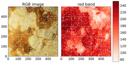
Figure 1Original photograph of the pancake used to generate the pancake dataset. The white points indicate the 500 sampling locations that were chosen randomly, without repeating. The observation value is the red-channel value of the RGB value of the specified pixel.
Neither the pancake nor the meuse dataset provide space-time data. To demonstrate the support of a space-time variogram within SciKit-GStat, another dataset of distributed soil temperature measurements was utilized and distributed with the software. The data are part of a dense network of cosmic-ray neutron sensors (Fersch et al., 2020), located in the Rott headwater catchment at the TERENO Pre-Alpine Observatory (Kiese et al., 2018) in Fendt, Germany. The distributed soil temperature measurements consist of “55 vertical profiles … covering an area of about 9 ha … record[ing] permittivity and temperature at 5, 20 and 50 cm depth, every 15 min.” (Fersch et al., 2020, Sect. 3.8.1, p. 2298). In order to decrease the computing demands, I only used temperature measurements at 20 cm and only used every sixth measurement.2
2.2 Package description
SciKit-GStat is a library for geostatistical analysis written in the Python programming language. The Python interpreter must be of version 3.6 or later. The source files can be downloaded and installed from the Python package index using pip, which is the standard tool for Python 3.3 All dependencies are installed along with the source files. This is the standard and recommended procedure for installing and updating packages in Python 3. Additionally, the source code is open and available on GitHub and can be downloaded and installed from source. SciKit-GStat is published under an MIT License.
The presented module is built upon common third-party packages for scientific computing in Python, called scipy.
In recent years, the SciPy ecosystem has become the de facto standard for scientific computing and applications in Python.
SciKit-GStat makes extensive use of numpy (Harris et al., 2020; van der Walt et al., 2011) to build data structures and numerical computations, matplotlib (Hunter, 2007) and plotly (Plotly Technologies Inc., 2015) for plotting, and the scipy library itself (Virtanen et al., 2020) for solving some specific mathematical problems, such as least squares or matrix operations.
An object-oriented programming approach was chosen for the entire library. SciKit-GStat is designed to interact with the user through a set of classes. Each step in a geostatistical analysis workflow is represented by a class and its methods. Argument names passed to an instance on creation are chosen to be as close as possible to existing and common parameter names from geostatistical literature. The aim is to make the usage of SciKit-GStat as intuitive as possible for geoscientists with only little or no experience with Python.
The main focus of the package is variogram analysis. Ordinary kriging is also implemented in SciKit-GStat but the main strength is variogram analysis. Kriging is available as a valuable tool to cross-validate the variogram by interpolating the observation values. For flexible, feature-rich and fast kriging applications, the variogram can be exported to other libraries with ease. SciKit-GStat offers an extensible and flexible class that implements common settings out of the box but can be adjusted to rather uncommon problems with ease. An example variogram is shown in Fig. 2. By default, the user has an experimental variogram, a well-fitted theoretical model and a histogram to estimate the point pair distribution in the lag classes at one's disposal. This way, the plot of the variogram instance helps the user, at first sight, to estimate not only the goodness of fit but also the spatial representativity of the variogram for the sample used. All parameters can be changed in place, and the plot can be updated, without restarting Python or creating new unnecessary variables and instances.
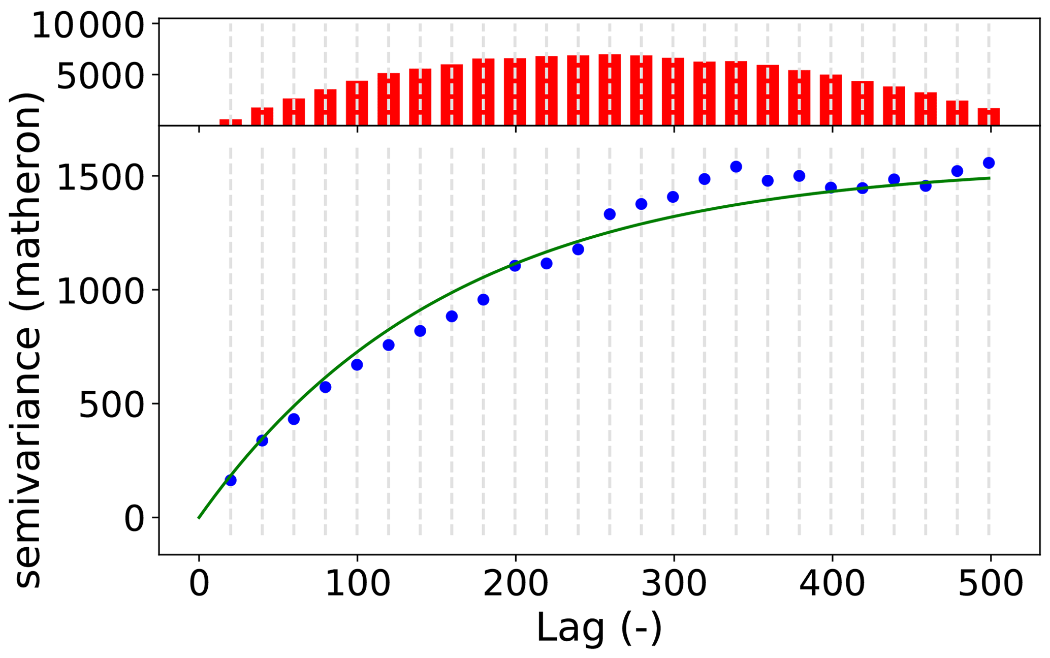
Figure 2Default variogram plot of SciKit-GStat using the matplotlib back end. The variogram was estimated with the pancake dataset using the exponential model (green line) fitted to an experimental variogram (blue dots) resolved to 25 evenly spaced lag classes, up to 500 units (the axis length of the sampled field). The histogram in the upper subplot shows the number of point pairs for each lag class. The histogram shares the x axis with the variogram to identify the corresponding lag classes with ease.
SciKit-GStat contains eight different semi-variance estimators (overview in Table 1) and seven different theoretical variogram model functions (overview in Table 2). At the same time, implementing custom models and estimators is supported by a decorator function that only requires the mathematical calculation from the user, which can be formulated with almost no prior Python knowledge, often with a single line of code.
Matheron (1963)Cressie and Hawkins (1980)Dowd (1984)Genton (1998)Shannon (1948)Table 1Overview of all semi-variance estimator functions implemented in SciKit-GStat. Using Normalized Range and Percentile is only advised to users understanding the implications as explained in Sect. 4.1.3.
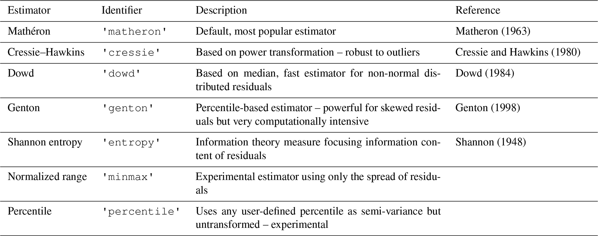
Table 2Overview of all theoretical variogram model functions implemented in SciKit-GStat.
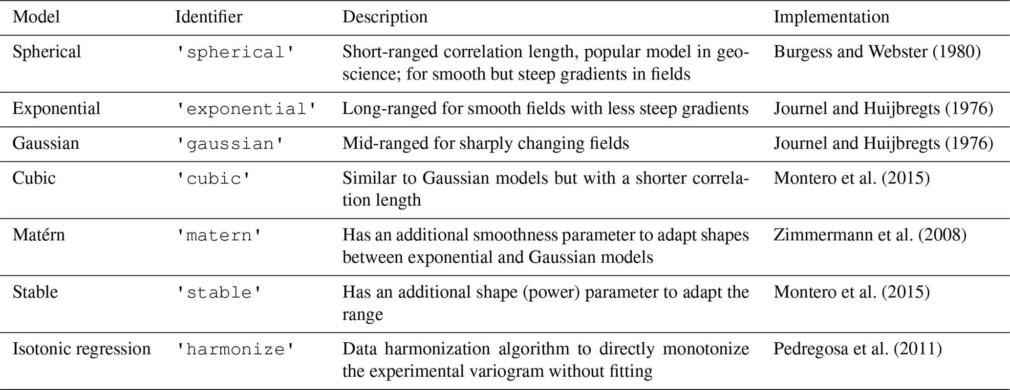
Table 3Overview of all lag class binning methods implemented in SciKit-GStat.
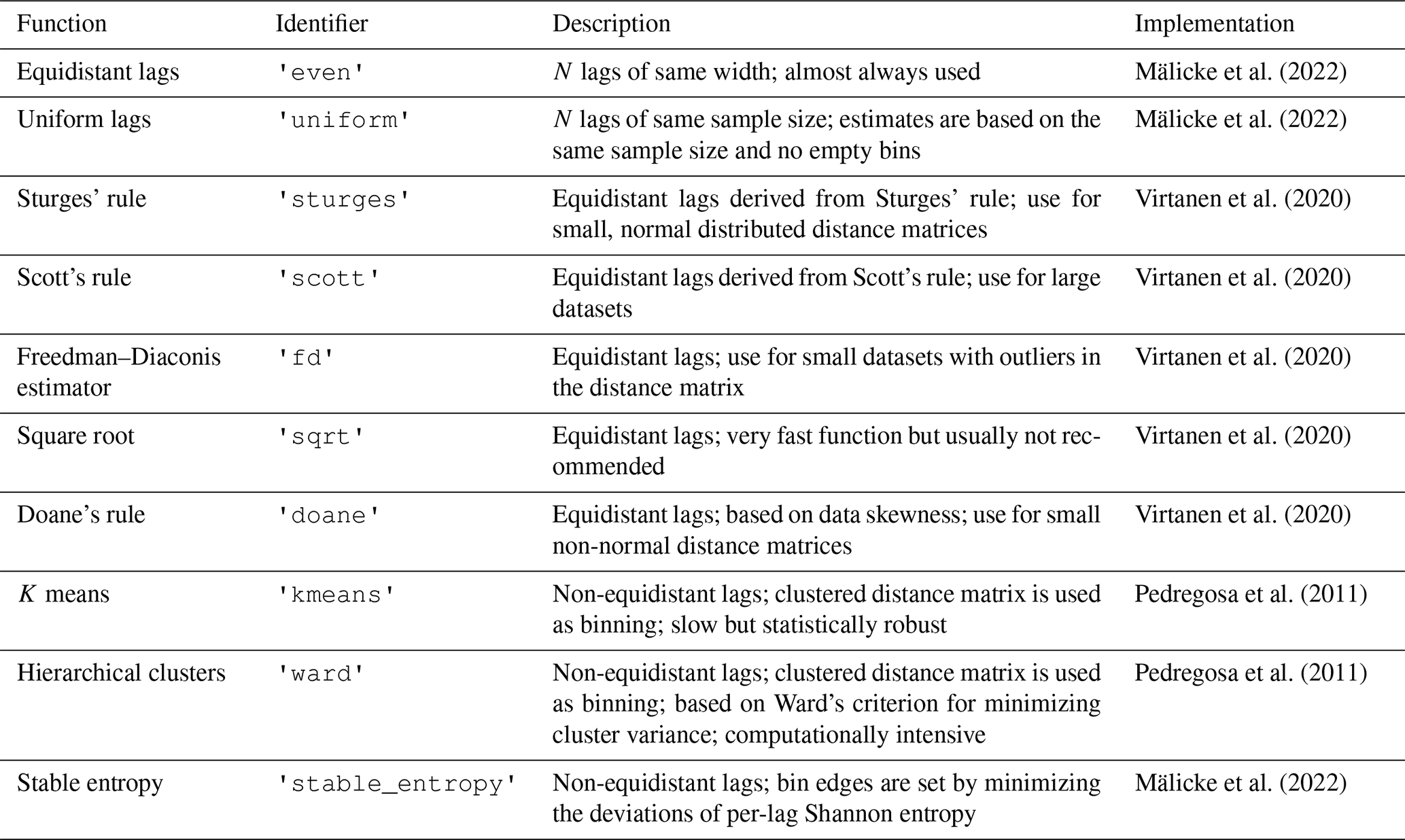
SciKit-GStat offers a multitude of customization options to fit variogram models to experimental data. The model parameters can be fitted manually or by one of three available optimization algorithms: Levenberg–Marquardt, trust-region reflective and parameter maximum likelihood (see Sect. 4.1.5). It is also possible to combine both fitting methods. Furthermore, it is possible to weight experimental data. Such weighting of experimental data is a crucial feature to make a variogram model fit data at short lags more precisely than distant observations. The user can manually adjust weights or use one of the many predefined functions that define weights, i.e., dependent on the separating distance. Closely related is the way SciKit-GStat handles spatial aggregation. The user can specify a function that will be used to calculate an empirical distribution of separating distance classes, which are the foundation for spatial aggregation. Especially for sparse datasets which base their aggregation on small sample sizes, even adding or removing a single lag class can dramatically change the experimental variogram. The default function defines equidistant distance lag classes, as mostly used in literature. However, SciKit-GStat also includes functionality for auto-deriving a suitable number of lag classes or cluster-based methods, which have, to my knowledge, not been used so far in this context. A complete overview of all functions is given in Table 3.
Interfaces for a number of other geostatistical packages are provided.
SciKit-GStat defines either an export method or a conversion function to transform objects that can be read by other packages.
Namely, Variogram can export a parameterized custom variogram function, which can be read by kriging classes of the pykrige package.
A similar export function can transform a variogram to a covariance model as used by gstools.
This package is evolving to be the prime geostatistical toolbox in Python. Thus, a powerful interface is of crucial importance.
Finally, a wrapping class for Variogram is provided that will make it accessible as a scikit-learn (Pedregosa et al., 2011) estimator object.
This way, scikit-learn can be used to perform parameter search and use variograms in a machine learning context.
SciKit-GStat is easily extensible. Many parts of SciKit-GStat were designed to keep the main algorithmic functions clean. Overhead like type checks and function mapping to arrays are outsourced to instance methods wherever possible. This enables the user to implement custom functions with ease, even if they are not too familiar with Python. As an example, implementing a new theoretical model is narrowed down to only implementing the mathematical formula this way.
Documentation provided with SciKit-Gstat is tailored for educational use. The documentation mainly contains a user guide, tutorials and a technical reference. The user guide for SciKit-GStat does not have any prerequisites in geostatistics and guides the reader through the underlying theory while walking through the implementation. Tutorials are provided for users with some experience with Python, geostatistics and other fields of statistics. The tutorials focus on a specific aspect of SciKit-GStat and demonstrate the application of the package. Here, a sound understanding of geostatistics is assumed. Finally, the technical reference only documents the implemented functions and classes from a technical point of view. It is mainly designed for experienced users that need an in-depth understanding of the implementation or for contributors that want to extend SciKit-GStat.
SciKit-GStat is 100 % reproducible through Docker images.
With only the Docker software installed (or any other software that can run Docker containers), it is possible to run the scikit-gstat Docker image, which includes all dependencies and common development tools used in scientific programming.
This makes it possible to follow the documentation and tutorials instantly.
The user can use a specific SciKit-GStat version (from 1.0 on) and conduct analysis within the container.
That will fix all used software versions and, if saved, make the analysis 100 % reproducible.
At the same time, the installation inside Docker container does not affect any existing Python environment on the host system and is therefore perfect to test SciKit-GStat.
SciKit-GStat is recognized on GitHub and has a considerable community.
Issues and help requests are submitted frequently and are usually answered in a short amount of time by the author.
At the same time, efforts are made to establish a broader developer community, to foster support and development.
Additionally, the development on SciKit-GStat is closely coordinated with gstools and the parenting GeoStat Framework developer community.
3.1 Variogram
In geostatistical literature, the terms semi-variogram and variogram are often mixed or interchanged. Although closely related, two different methods are described by these terms. In most cases, the semi-variogram is used, but called simply variogram. Here, I follow this common nomenclature, and both terms describe the semi-variogram in the following.
At its core, the semi-variogram is a means to express how spatial dependence in observations changes with separating distance. An observation is here defined to be a sample of a spatial random function. While these functions are usually two- or three-dimensional functions in geostatistical applications, they can be N dimensional in SciKit-GStat (including 1D). A more comprehensive and detailed introduction to random functions in the context of geostatistics is given in Montero et al. (2015, chap. 2.2, p. 11 ff.). Therefore, the most fundamental assumption that underlies a variogram is that proximity in space leads to similar observations (proximity in value). To calculate spatially aggregated statistics on the sample, the variogram must make an assumption up to which distance two observations are still close in space. This is carried out by using a distance lag over the exact distances, as two point pairs will hardly be at exactly the same spatial distance in real-world datasets.
Separating distance is calculated for observation point pairs. For different distance lag classes (e.g., 10 to 20 m), all point pairs si, sj within this class are aggregated to one value of (dis)similarity, called semi-variance γ. A multitude of different estimators are defined to calculate the semi-variance. For a specific lag distance h (e.g., 10 m), the most commonly used Matheron estimator (Matheron, 1963) is defined by Eq. (1):
where N(h) is the number of point pairs for the lag h, and Z(s) is the observed value at the respective location s. The obtained function is called an experimental variogram in SciKit-GStat. In literature, the term empirical variogram is also quite often used and is referring, more or less to the same thing. In SciKit-GStat, the empirical variogram is the combination of the lag classes and the experimental variogram. All estimators implemented in SciKit-GStat are described in detail in Sect. 4.1.3.
To model spatial dependencies in a dataset, a formalized mathematical model has to be fitted to the experimental variogram. This step is necessary, to obtain parameters from the model in a formalized manner. These describe spatial statistical properties of the model, which may (hopefully) be generalized to the random field. These parameters are called variogram parameters and include the following:
-
nugget – the semi-variance at lag h=0. This is the variance that cannot be explained by a spatial model and is inherit to the observation context. (i.e., measurement uncertainties or small-scale variability).
-
sill – the upper limit for a spatial model function. The nugget and sill add up to the sample variance.
-
effective range – the distance, at which the model reaches 95 % of the sill. For distances larger than the range, the observations become statistically independent. Variogram model equations also define a model parameter called range, which leads to misunderstandings in the geostatistical community. To overcome these problems, SciKit-GStat formulated all implemented models based on the effective range of the variogram and not the range model parameter. Consequently, the given formulas might differ from some common sources by the transformation of effective range to range model parameter. These transformations are straightforward and reported in literature, but for some models (i.e., Gaussian) they are not commonly the same. In these cases, the user is encouraged to carefully check the implementation used in SciKit-GStat.
Closely related to these parameters is the nugget-to-sill ratio. It is interpreted as the share of spatially explainable variance in the sample and is therefore a very important metric to reject the usage of a specific variogram model at all.
The theoretical model is a prerequisite for spatial interpolation. For this to happen, a number of geostatistical assumptions need to be fulfilled. Namely, the observations have to be of second-order stationarity, and the intrinsic hypothesis has to hold. This can be summarized as the requirement that the expected value of the random function and its residuals must not be dependent on the location of observation but solely on the distance to other points. This assumption has to hold for the full observation space. Hence, the semi-variance is calculated with the distance lag h as the only input parameter. A more detailed description of these requirements is given in Montero et al. (2015, chap. 3.4.1, p. 27 ff.) or Burgess and Webster (1980) and Bárdossy and Lehmann (1998). An important tool to learn about trends in the input dataset is a scatterplot like that shown in Fig. 3. The same variogram instance that was used for Fig. 2 is used here. The two panels show the observation values related to only one dimension of their coordinates. This scatterplot can help the user to identify a dependence of observations on the location, which could violate the assumptions named above. The pancake sample observations are independent of the x axis coordinates (1-dimension). For the second dimension, there might be a slight dependence of large observation values on the y coordinate. This readily available plot is useful to guide the user into the decision of utilizing statistical trend tests to test for statistical significance and finally detrending input data.
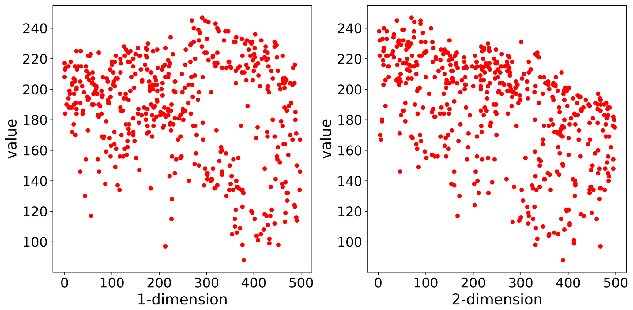
Figure 3Scatterplot of the observation values in the pancake dataset related to only one coordinate dimension. As the pancake dataset was 2D, 1-dimension corresponds to the x coordinate and 2-dimension to the y coordinate of the pancake sample. This plotting procedure can help the user to identify a dependence on the location for the data sample, which can violate the second-order stationarity.
The other requirement for variogram models is that it has to be monotonically increasing. A drop in semi-variance would imply that observations become more similar with increasing distance, which is incompatible with the most fundamental assumption in geostatistics of spatial proximity. This requirement can only be met by a statistical model function and not the experimental variogram, which is often not monotonically increasing in a strict sense. This may happen due to the fact that (spatial) observations are not exhaustive and measurements might be uncertain.
3.2 Kriging
One of the most commonly used applications of geostatistics is kriging. A sample result is shown in Fig. 4. The interpolation was made with the same variogram instance used to produce Figs. 2 and 3. The center panel shows the result itself, along with the original field (left panel) and a kriging error map (right panel), which will be introduced later. In this example, the spatial properties and correlation lengths of the original are well captured by the result.
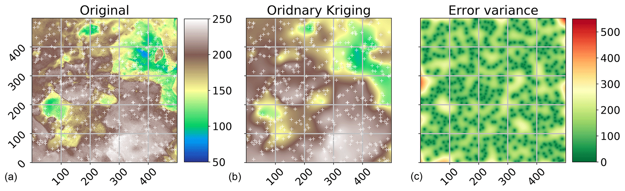
Figure 4Ordinary kriging result of the pancake dataset sample used in Figs. 2 and 3. The kriging was performed with default parameters on a grid of the same resolution as the original field. The original image and ordinary kriging result share the value space; thus, the color bar between the two panels (a, b) is valid for both. The original is the same as in Fig. 1 but using a different color scale to make differences more pronounced. The white crosses indicate the sample positions. The third panel (c) indicates the associated kriging error variance as returned by the algorithm.
Kriging estimates the value for an unobserved location s0 as the weighted sum of nearby observations as shown in Eq. (2).
where Z*(s0) is the estimation, and λi represents the weights for the N neighbors si. The kriging procedure uses the theoretical variogram model fitted to the data to derive the weights from the spatial covariance structure. Furthermore, by requiring all weights to sum up to one (Eq. 3), the unbiasedness of the prediction is assured.
A single weight can thereby be larger than one or smaller than zero. As the weights are inferred from the spatial configuration of the neighbors, this can require stronger influence (λ>1) or even negative influence (λ<0) of specific observations. Combined with unbiasedness, this is one of the most important features of a kriging interpolation and can make it superior to, for example, spline-based procedures in an environmental context. Deriving weights from the spatial properties of the data is especially helpful, as the local extreme values have likely not been observed, but their influence is present in the spatial covariance of the field close to it.
To obtain the weights for one unobserved location, a system of equations called the kriging equation system (KES) is formulated. By expecting the prediction errors to be zero (Eq. 4) and substituting Eq. (2) in Eq. (4), the KES can be formulated.
The final kriging, Eq. (5), is taken from Montero et al. (2015, Eq. 4.16, p. 86), and its derivation is given in chap. 4.3.1 of the same source (Montero et al., 2015, pp. 84–90).
where α is the Lagrange multiplier needed to solve the KES by minimizing the estimation variance subject to the constraint of Eq. (3). By minimizing the prediction variance and requiring the weights to sum to one, it is possible to obtain the best linear, unbiased estimation. Thus, kriging is often referred to as being a BLUE (Best Linear Unbiased Estimator). Using kriging, an estimate of the variance of the spatial prediction can be obtained. This is shown in the right panel of Fig. 4. Such information is vital to assess the quality of the prediction. Finally, the setup of kriging makes it a smooth interpolation, as the predictions very close to observation locations are approaching the observation values smoothly. The kriging variance is significantly higher in less densely sampled regions (Fig. 4), which enables the user to visually assess the spatial representativity of the obtained results.
3.3 Directional variogram
The standard variogram as described in Sect. 3.1 handles isotropic samples. That means the spatial correlation length of the random field is assumed to be of comparable length in each direction. Usually, one refers only to the directions along the main coordinate axes. However, direction can be defined with any azimuth angle and does not have to match the coordinate axes. If the spatial correlation length differs in direction this is referred to as anisotropy. There are two different kinds of anisotropy: geometric and zonal anisotropy (Wackernagel, 1998). Considering geometric anisotropy, the effective range differs for the two perpendicular main directions of the anisotropy. In the zonal case, sill and range differ. Geometric anisotropy can be handled by a coordinate transformation (Wackernagel, 1998). These cases can be detected by directional variograms. For an application, the main directions of anisotropy must be identified to then estimate an isolated variogram for each direction.
For each directional variogram, only point pairs are considered that are oriented in the direction of the variogram. For two observation locations s1 and s2, the orientation is defined as the angle between the vector u connecting s1 and s2 and a vector along the first dimension axis: . The cosine of the orientation angle Θ can be calculated using Eq. (6):
The directional variogram finally defines an azimuth angle, defined analogous to Eq. (6), and a tolerance. Any point pair which deviates less than tolerance from the azimuth is considered to be oriented in the direction of the variogram and will be used for estimation.
The example data used so far shows a small anisotropy (Fig. 5). The two variograms used exactly the same data and parameters as used for Fig. 2. The only difference is that both are directional, and they use two different directions of 0 and 90∘. There is a difference in effective range and sill in the 90∘ directional variogram.

Figure 5Two directional variograms calculated for the pancake dataset. Both variograms use the same parameters as the instance used to produce Fig. 2. In addition, the direction is taken into account. The two variograms shown differ only in the azimuth used, which is 0∘ (a) and 90∘ (b).
As long as more than one directional variogram is estimated for a data sample, the difference in the estimated variogram parameters describes the degree of anisotropy.
In a kriging application, the data sample can now be transformed along the main directions at which the directional variograms differ until the directional variograms do not indicate an anisotropy anymore.
The common variogram of the transformed data can be used for kriging, and the interpolated field is finally transformed back.
Transformations are not part of SciKit-GStat. The scipy and numpy packages offer many approaches to apply transformations.
Alternatively, gstools implements anisotropy directly and can use it for covariance models and kriging. In these cases, the user needs to identify the directions manually and specify them on object creation.
3.4 Space-time variogram
At the turn of the millennium, geostatistics had emerged as a major tool in environmental science and geoscience, and the demand for new methods was rising. Datasets collected in nature are usually dynamic in time, which can easily violate the second-order stationarity assumptions underlying classic geostatistics. Hence, substantial progress had been made to incorporate temporal dimensions into variograms.
The classic variogram is modeling the semi-variance of a sample as a function of the separating distance of the underlying point pairs. For a space-time variogram, this dependence is expanded to time lags. That means the data are segmented not only in terms of spatial proximity but also temporal proximity. The resulting model will be capable of identifying covariances over space and time at the same time (Fig. 6). SciKit-GStat uses a 3D plot by default. The plot can be customized and exclude the fitted model or plot the experimental variogram as a surface rather than a scatterplot. While Fig. 6 might contain both the experimental and the theoretical variogram, it is also quite overloaded and not always helpful. Finally, a printed 3D plot cannot be rotated, and the usage in publications is discouraged. To overcome these limitations, SciKit-GStat implements 2D contour plots of the experimental variogram in two variations, which differ only in visualization details (Fig. 7). The contour plot is the more appropriate means to inspect the covariance field as estimated by the space-time variogram. With the given example, one can see that the auto-correlation (temporal axis) is dominant, and except for a few temporal lags (50–60 or 30–40), the variogram shows almost a pure nugget along the spatial axis. Note that the contour lines smooth out the underlying field to close lines to rings wherever possible. This can lead to the impression that the experimental variogram is homogeneously smooth along the two axes. In fact, this is not the case, and the smoothing is due to the implementation of contour lines. Thus, the contour plot should be used to get a general idea of the experimental variogram. To inspect the actual semi-variance values, the experimental variogram can be accessed and plotted using a matrix plot.
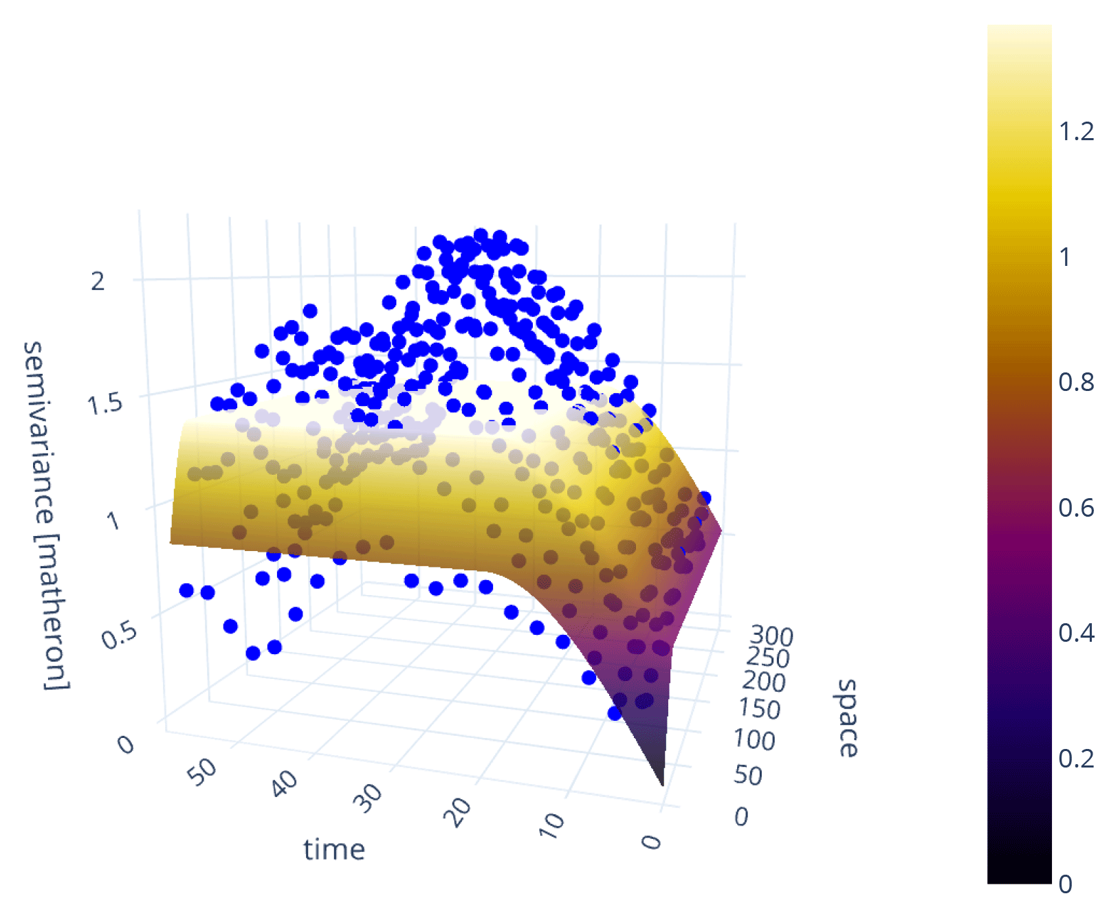
Figure 6Default 3D scatterplot of a space-time variogram (blue points), with fitted product-sum model (surface). The variogram is estimated from the in situ soil temperature measurements at 20 cm depth (WSN product, Wireless Sensor Network) published in Fersch et al. (2020). To decrease the computational workload, only every sixth measurement was taken from the time series.
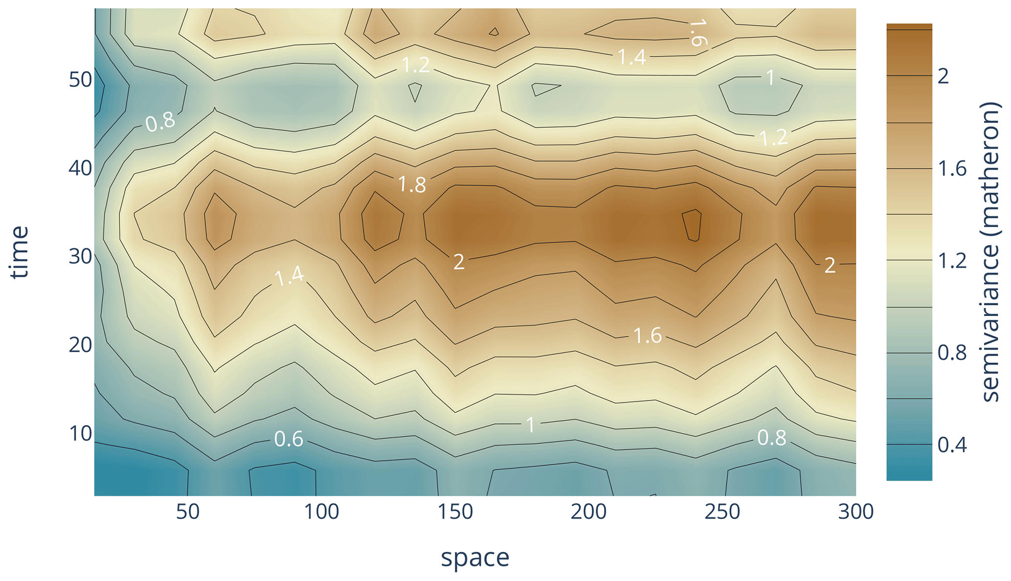
Figure 7Contour plot of an experimental space-time variogram, without theoretical model. The shown variogram is from exactly the same instance as used for Fig. 6, without any modifications. The contours are calculated for the semi-variances (z axis) and thus contain the same information as the scatterplot in Fig. 6. The color is indicating the magnitude of the semi-variance according to the color bar.
To build a separable space-time variogram model, the two dimensions are first calculated separately. Non-separable space-time variogram models are not covered in SciKit-GStat. The two experimental variograms are called marginal variograms and relate to the temporal or the spatial dimension exclusively, by setting the other dimension's lag to zero. Finally, these two variograms are combined into a space-time variogram model. SciKit-GStat implements three models: the sum model, product model and product-sum model. For each of the marginal experimental variograms, a theoretical model is fitted, as described in Sect. 3.1. These two models Vx(h) (spatial) and Vt(t) (temporal) are then used to combine their output into the final model's return value γ. The space-time model defines how this combination is archived.
For the sum model, γ is simply Vx(h)+Vt(t). The product and product-sum models are implemented following De Cesare et al. (2002, Eqs. 4 and 6).
This section focuses on the implementation of SciKit-GStat. It aims to foster an understanding of the most fundamental design decisions made during development. Thus, the reader will gain a basic understanding of how the package works, where to get started and how SciKit-GStat can be extended or adjusted.
4.1 Main classes
SciKit-GStat is following an object-oriented programming (OOP) paradigm.
It exports a number of classes, which can be instantiated by the user.
Common geostatistical notions are reflected by class properties and methods to relate the lifetime of each object instance to typical geostatistical analysis workflows.
At the core of SciKit-GStat stands the Variogram class for variography.
Other important classes are the following:
-
DirectionalVariogramfor direction-dependent variography, -
SpaceTimeVariogramfor space-time variography, -
OrdinaryKrigingfor ordinary kriging interpolations.
4.1.1 Variogram
The Variogram is the main class of SciKit-GStat and the only construct the user will interact with, in most cases.
Each instance of this class represents the full common analysis cycle in variography.
That means each instance will be associated with a specific data sample and holds a fitted model.
Other than other libraries, there is no abstraction of variogram models, and fitted models are not an entity of their own.
If alternate input data (not parameters) are used, a new object must be created.
This makes the transfer of variogram parameter onto other data samples a conscious action performed by the user and not a side effect of the implementation.
At the same time, parameters are mutable and can be changed at any time, which will cause recalculation of dependent results.
While this design decision makes the usage of SciKit-GStat straightforward, it can also decrease performance.
That is, in SciKit-GStat, a variogram model is always fitted, even if only the experimental variogram is used.
This can be a downside, especially for large datasets.
For cases where the full variogram instance is not desired or needed, possible pathways are described in Sect. 4.1.3 and 4.1.4, but the usage of gstools might be preferable in these cases.
The second design decision for Variogram was interactivity.
To take full advantage of OOP, every result, parameter and plot are accessible as an instance attribute, property or method.
This always clearly sets ownership and provenance relations for data samples and derived results and properties, as there are no floating results that have to be captured in arbitrarily named variables.
Moreover, parameters that might be changed during a variogram analysis are implemented in a mutable way. Substantial effort was made to store as few immutable parameters as possible in the instance.
Thus, whenever a parameter is changed at runtime, depending derived attributes and results will be updated.
This convenient behavior for analysis comes at the cost of performance.
This is another major difference to the gstools library, in which the author assumes performance to be a driving design decision.
To illustrate this as an example, the following is given. When a variogram instance is constructed without further specifying the spatial model that should be used, it will default to the spherical model.
The instance is fitted to this model after construction and can be inspected by the user, i.e., by calling a plot method.
The user wants to check out another semi-variance estimator, such as the Cressie–Hawkins estimator, because there are a lot of outliers in the dataset.
Changing the estimator is as easy as setting the literal estimator name to the estimator property of the variogram.
The experimental variogram will instantly be dropped and recalculated as well as all depending parameters, such as the variogram parameters.
The spherical model is fitted a second time now.
The user might then realize that a spherical model is not suitable and can simply change the model attribute, i.e., to the Matérn model.
As a direct effect, the variogram parameters are dropped again, as they are once again invalidated, and a new fitting procedure is invoked.
This behavior is extremely convenient, as it is easy, interactive, expressive and instant.
But it is also slow, as the theoretical model had been fitted three times before the user even looked into it.
To add some context to slow calculations, an experimental variogram estimation runtime test4
has been performed (Fig. 8).
One can see that SciKit-GStat and gstools are very comparable in this case, and both are significantly faster than a native Python implementation, especially for larger datasets.
Note the log-scaled y axis, indicating differences of magnitudes for larger sample sizes.
Interactively adjusting variogram parameters will invoke additional calculations of given runtimes.
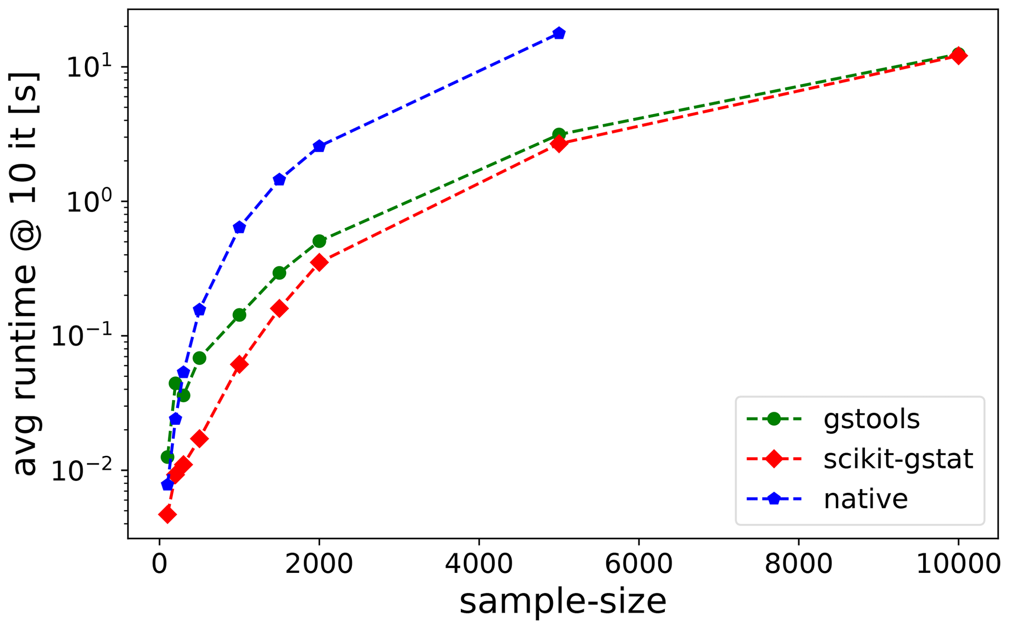
Figure 8Benchmark test for estimating an experimental variogram. For each sample size, the mean runtime of 10 repetitions is shown. The experimental variogram was calculated with a native Python implementation (blue), gstools (green) and SciKit-GStat (red).
Although most attributes are mutable, they use common data types in their formulation.
This enables the user to interrupt the calculation at any point using either primitive language types or numpy data types, which are most accepted by the scientific community as the prime array and matrix data types.
Thus, there is no need for the user to learn about custom data, parameter or result structures using SciKit-GStat.
4.1.2 Distance lag classes
Possibly the most crucial step to estimate a suitable variogram is the binning of separating distances into distance lag classes. In some parts, SciKit-GStat also includes information theory methods. Here, to calculate the basic measure, Shannon entropy (Shannon, 1948), the input data have to be binned to calculate empirical non-exceeding probabilities. To distinguish the information theory binning from the procedure of binning separating distances into classes, I will refer to the latter as lag classes. In the literature, lag classes are commonly referred to as bins, lags, distance lags or distance bins.
SciKit-GStat implements a large number of methods to form lag classes.
They can be split into two groups. Some are adjusting class edges to fit the requested number of lag classes.
The other group will adjust the number of lag classes to fit other statistical properties of the resulting lag classes.
All methods can be limited by a maximum lag. This is a hyper-parameter that can be specified by the user but is not set by default.
There are various options for the maximum lag. The user can set the parameter by an absolute value, in coordinate units and larger than one.
Alternatively, a number between 0 and 1 can be set.
Then, the Variogram class will set the maximum lag to this share of the maximum pairwise distance found in the distance matrix.
That is, if 0.5 is used, the maximum lag is set to half of the largest point pair distance found. Note that this is not a median value.
Finally, a string can be set as maximum lag. This can request either the arithmetic mean or the median value of the distance matrix as the maximum lag.
Typical values from geostatistical textbooks are the median or 60 % of the maximum lag (value of 0.6 in SciKit-GStat).
The default behavior is to form a given number of equidistant lag classes, from 0, to the maximum lag distance. This procedure is used in the literature in almost all cases (with different max lags) and is thus a reasonable default method.
Another procedure takes the number of lag classes and forms lag classes of uniform size. That means each lag class will contain the same number of point pairs and thus be of varying width. This procedure can be explicitly useful to avoid empty lag classes, which can easily happen for equidistant lag classes. Another advantage is that the calculation of semi-variance values will always be based on the same sample size, which makes the values statistically more comparable. These advantages come at the cost of less comparable lag classes. Care must be taken when interpreting lag-related variogram properties such as the effective range. There might be lag ranges that are supported by only a very low number of actual lag classes.
The next group of procedures use common methods from histogram estimation to calculate a suitable number of lag classes. This is carried out either directly or by estimating the lag class width and deriving the number of classes needed from this.
The first option is to apply Sturges' rule (Scott, 2009) as shown in Eq. (7):
where s is the sample size, and n is the number of lag classes. This rule works good for small, normally distributed distance matrices but often yields too small n for large datasets.
Similar to Sturges' rule, the square-root rule estimates the number of lag classes as given in Eq. (8):
This rule is not recommended in most cases. It comes with similar limitations as Sturges' rule, but in contrast, it usually yields too large n for large s. The main advantage of this rule is that it is computationally by far the fastest of all implemented rules.
Scott's rule (Scott, 2010) does not calculate n directly but rather h, the optimal width for the lag classes using Eq. (9):
where σ is the standard deviation of s. By taking σ into account, Scott's rule works well for large datasets. Its application does not work very well on distance matrices with outliers, as the standard deviation is sensitive to outliers.
If Scott's rule does, due to outliers, not yield suitable lag classes, the Freedman–Diaconis estimator (Freedman and Diaconis, 1981) can be used. This estimator is similar to Scott's rule, but it makes use of the interquartile range as shown in Eq. (10):
The interquartile range (IQR) is robust to outliers, but in turn the Freedman–Diaconis estimator usually estimates way too many lag classes for smaller datasets. The author cannot recommend to use it for distance matrices with less than 1000 entries.
Finally, Doane's rule (Doane, 1976) is available. This is an extension to Sturges' rule that takes the skewness of the sample into account. This makes it especially suitable for smaller, non-normal datasets, where the other estimators do not work very well. It is defined as given in Eq. (11):
Here, g is the skewness, σ is the standard deviation, μg is the arithmetic mean and x is each element in s.
All rules that calculate the number of lag classes use the numpy implementation of the respective methods (van der Walt et al., 2011).
All histogram estimation methods given above just calculate the number of lag classes. The resulting classes are all equidistant, except for the first lag class, which has 0 as a lower bound instead of min(s).
Finally, SciKit-GStat implements two other methods. Both are based on a clustering approach and need the number of lag classes to be set by the user. The distance matrix is clustered by the chosen algorithm. Depending on the clustering algorithm, the cluster centers (centroids) are either estimates of high density or points in the value space, where most neighboring values have the smallest mean distance. Thus, the centroids are taken as a best estimate for lag class centers. Each lag class is then formed by taking half the distance to each sorted neighboring centroid as bounds. This will most likely result in non-equidistant lag classes.
The first option is to use the K-means clustering algorithm, which is maybe the most popular clustering algorithm. The method is often attributed to MacQueen (1967), but there are thousands of variations and applications published.
The implementation of K means used in SciKit-GStat is taken from scikit-learn (Pedregosa et al., 2011).
One important note about K-means clustering is that it is not a deterministic method, as the starting points for clustering are taken randomly.
In practice, this means that exactly the same Variogram instantiated twice can result in different lag classes.
Experimental variograms are very sensitive to the lag classes. In some unsystematic tests undertaken by the author, the variations in lag class edges could be as large as 5 % of the distance matrix range, which would result in substantially different experimental variograms.
Thus, the decision was made to seed the random start values.
For this reason, the K-means implementation (denoted K-Means hereafter) in SciKit-GStat is deterministic and will always return the same lag classes for the same distance matrix.
The downside is that the clustering loses some of its flexibility and cannot be cross-validated.
Additionally, the K-Means might not converge. In these cases the Variogram class raises an exception and invalidates the variogram.
Furthermore, the K-Means will find one set of lag classes but not necessarily the best one.
However, the user can still calculate lag class edges externally, using K-Means, and pass the edges explicitly to the Variogram class.
The other clustering algorithm is a hierarchical clustering algorithm (Johnson, 1967). These algorithms group values together based on their similarity. SciKit-GStat uses an agglomerative clustering algorithm, which uses Ward's criterion (Ward and Hook, 1963) to express similarity. Agglomerative algorithms work iteratively and deterministic, as at first iteration each value forms a cluster on its own. Each cluster is then merged with the most similar other cluster, one at a time, until all clusters are merged or the clustering is interrupted. Here, the clustering is interrupted as soon as the specified number of classes is reached. The lags are then formed similar to the K-Means method, either by taking the cluster mean or median as center. Ward's criterion defines the one other cluster as the closest, which results in the smallest intra-cluster variance for the merged clusters. That finally results in slightly different lag class edges than K-Means. The main downside of agglomerative clustering is that it is by far the slowest method. In some cases, especially for larger datasets, the clustering took longer than the full workflow to estimate a variogram and fit a theoretical model by magnitudes.
The implementation follows scikit-lean (Pedregosa et al., 2011), using the AgglomerativeClustering class with the linkage parameter set to 'ward'.
One method of utilizing clustered lag classes is to compare the K-Means lag edges with the default settings. The idea is to minimize the deviation of both while searching a suitable number of classes. This combines the advantages of K-Means while yielding equidistant lag classes that have the best match to clustered centroids. SciKit-GStat makes that possible while leaving the interpretation to the user.
Another option available is called stable entropy.
This is a custom optimization algorithm that has not been reported before.
The algorithm takes the number of lag classes as a parameter and starts with the equidistant lag classes as an initial guess for optimization.
It seeks to adjust bin edges until all lag classes show a comparable Shannon entropy.
Shannon entropy is calculated using Eq. (15), with a static binning created analogous to Eq. (8) and the square-root rule for histogram estimation.
The lag classes are optimized by minimizing the absolute deviation in Shannon entropy, at a maximum of 5000 iterations.
The algorithm uses the Nelder–Mead optimization (Gao and Han, 2012) implemented in scipy (Virtanen et al., 2020).
As the Shannon entropy is a measure of uncertainty based on information content, it is expected to yield statistically robust lag classes.
At the same time, it is expected to show the same limitations as the uniformly sized lag classes, such as a potentially difficult interpretation of variogram parameters.
4.1.3 Sub-module: estimators
SciKit-GStat implements a number of semi-variance estimators. It includes all semi-variance estimators that are commonly used in the literature.
The numba package offers function decorators that enable just-in-time compilation of Python code.
Although there are ways to compile code even more effectively (i.e., Cython, Nuitka packages), numba comes at zero implementation overhead and fair calculation speedup.
The numba decorator is implemented for the matheron, cressie, entropy and genton estimators.
For the other estimators, the just-in-time compilation adds more compiling overhead than a compiled version actually gains on reasonable data sample sizes.
The main reason is that the remaining estimators are already covered mathematically by a numpy function, which are in most cases already implemented in a compiled language.
The matheron function implements the Mathéron semi-variance γ (Matheron, 1963). This estimator is so commonly used that it is often referred to just as semi-variance and thus the obvious default estimator in SciKit-GStat.
It is defined in Eq. (1).
cressie implements the Cressie–Hawkins estimator γc (Cressie and Hawkins, 1980).
As given in Eq. (12),
where N(h) is the number of point pairs s, si at separating lag h, and Z(s) is the observation value at s.
dowd implements the Dowd estimator γD (Dowd, 1984).
As given by Eq. (13),
This estimator is based on the median value of all pair-wise differences si, si+h separated by lag h, where Z(s) is the observation value at location s. Thus, the Dowd estimator is very robust to outliers in the pair-wise differences and very fast to calculate.
genton implements the Genton estimator γG (Genton, 1998).
As given by Eq. (14),
where the pair-wise differences Z(si), Z(sj) at separating lag h are only used if i<j. The nth percentile is calculated from k and q, which are both binomial and only depend on the number of point pairs N(h). The implementation in SciKit-GStat simplifies the application of the equation by setting for N(h)≧500. This avoids the necessity to solve very large binomials at negligible errors, as . The author has found the Genton estimator to yield a reasonable basis for variogram estimation in many environmental applications (a personal, maybe biased, observation). However, calculating the binomials requires some time. Especially if there are a lot of lag classes and a considerable number of them do not fulfill the N(h)≧500 constraint, this will slow down the calculation by many magnitudes compared to the other estimators.
minmax implements a custom estimator.
The author is unaware of any publication on this estimator. It was introduced during development, as it has quite predictable statistical properties.
However, I am also unaware of any useful practical applications of this estimator and can thus not recommend using it in typical geostatistical analysis workflows.
The MinMax estimator divides the value range of pairwise differences by their mean value.
entropy is an implementation of the Shannon entropy H (Shannon, 1948) as a semi-variance estimator.
A successful application of Shannon entropy as a measure for similarity as a function of spatial proximity has been reported by Thiesen et al. (2020).
Shannon entropy is defined with Eq. (15):
where pi is the empirical exceeding probability of for each separating lag h.
To calculate the empirical probabilities of occurrence, a histogram of all pairwise differences is calculated.
This histogram has evenly spaced bin edges, and the user can set the number of bins as a hyper-parameter to entropy.
Alternatively, the bin edges can be set explicitly.
One has to be aware that Shannon entropy relies on a suitable binning of the underlying data.
This might need some preliminary examination of , which is readily accessible as a property.
It is highly recommended to use exactly the same bin edges for all separating distances h needed to process a single variogram.
Otherwise the entropy values and their gradient over distance are not comparable, and the whole variogram analysis turns meaningless.
Finally, it is possible to use custom, user-defined functions for estimating the semi-variance.
The function has to accept a one-dimensional array of pair-wise differences, as these are already calculated by the Variogram class.
The return value must be a single, floating-point value. This can either be the primitive Python type or a 64-bit numpy float.
The given function is finally mapped to all separating distance lags automatically, thus there is no need to implement any overhead, such as sorting or grouping, by the user.
This empowers users with little or no experience with Python to define new semi-variance estimators as only the mathematical description of the semi-variance is needed as Python code.
4.1.4 Sub-module: models
SciKit-GStat implements a number of theoretical variogram models. The most commonly used models from literature are available. However, during researching theoretical models, the author brought an almost limitless number of models or variations thereof to light. Thus, the process of implementing new models was eased as far as possible instead of implementing anything that could be useful. Any variogram model function (implemented or custom) will receive the effective range as a function argument and is fitted using it. In the case when the mathematical model of a variogram function uses the range parameter, one has to implement the conversion into the model function as well.
The core design decision for SciKit-GStat's theoretical variogram models was to implement a decorator that wraps any model function. This decorator takes care of handling input data and aligning output data. Thus, the process of implementing new variogram models is simplified to writing a function that maps a single given distance lag to the corresponding semi-variance value.
Each model will receive the three variogram parameter effective range, sill and nugget as function arguments.
The nugget is implemented as an optional argument with a default value of zero, in the case when the user disables the usage of a nugget in the Variogram class.
Custom variogram models have to reflect that behavior.
spherical is the implementation of the spherical model, which is one of the most commonly used variogram models.
Thus, the spherical variogram model is the default model, in the case when the user did not specify a model explicitly.
The model equation is taken from Burgess and Webster (1980) and given in Eq. (16):
where h is the distance lag, and b, C0 and a are the variogram model parameters: nugget, sill and range. The range of a spherical model is defined to be exactly the effective range r.
exponential is the implementation of the exponential variogram model.
The implementation is taken from Journel and Huijbregts (1976) and given in Eq. (17):
where h is the distance lag, and b, C0 and a are the variogram model parameters: nugget, sill and range. For the exponential model, the effective range r is different from the variogram range parameter a.
gaussian is the implementation of the Gaussian variogram model.
The implementation is taken from Journel and Huijbregts (1976) and given in Eq. (18):
where h is the distance lag, and b, C0 and a are the variogram model parameters: nugget, sill and range. For the Gaussian model, the effective range r is different from the variogram range parameter a. In SciKit-GStat, the conversion from effective range to range parameter is implemented as shown in Eq. (18). However, the author is aware of other implementations in the literature. The package does not allow users to somehow switch the conversion, and the user has to implement a new Gaussian model in the case when another conversion is desired.
cubic is the implementation of the cubic variogram model.
The implementation is taken from Montero et al. (2015) and given in Eq. (19):
where h is the distance lag, and b, C0 and a are the variogram model parameters: nugget, sill and range. For the cubic model, the effective range r is exactly the variogram range parameter a.
matern in the implementation of the Matèrn variogram model.
The implementation is taken from Zimmermann et al. (2008) and given in Eq. (20):
where h is the distance lag, Γ is the gamma function, and b, C0 and a are the variogram model parameters: nugget, sill and range. Additionally, the Matérn model defines a fourth model parameter υ, which is a smoothness parameter. For the Matérn model, the effective range a is a fraction of the variogram parameter range r.
stable is the implementation of the stable variogram model.
The implementation is taken from Montero et al. (2015) and given in Eq. (21):
where h is the distance lag, and b, C0 and a are the variogram model parameters: nugget, sill and range. Additionally, the stable model has a shape parameter s. The effective range of the variogram is a fraction of the variogram range parameter, dependent on this shape. Generally, the effective range will increase with larger shape values.
harmonize is an implementation that is rather uncommon in geostatistics.
It is based on the idea of monotonizing a data sample into a non-decreasing function.
That means there is no model fitting involved, and the procedure bypasses all related steps.
A successful application in geoscience was reported by Hinterding (2003).
For SciKit-GStat, the more generalized approach of isotonic regression (Chakravarti, 1989) was used which is already implemented in scikit-learn (Pedregosa et al., 2011).
Note that a harmonized model might not show an effective range, in which cases the library will take the maximum value as the effective range for technical reasons.
Thus, the user has to carefully double-check harmonized models for their geostatistical soundness.
Secondly, the harmonized model cannot be exported to gstools, which makes it unavailable for most kriging algorithms.
4.1.5 Fitting theoretical models
As soon as an estimated variogram is used in further geostatistical methods, such as kriging or field simulations, it is necessary to describe the experimental, empirical data by a model function of defined mathematical properties. That is, for kriging, a variogram has to be monotonically increasing and positive definite. This is assured by fitting a theoretical model to the experimental data. The models available in SciKit-GStat are described in Sect. 4.1.4.
Fitting the theoretical model to the experimental data is crucial, as any uncertainty caused by this procedure will be propagated to any further usage of the variogram.
Almost any geostatistical analysis workflow is based on some kind of variogram; hence, the goodness of fit will influence almost any analysis.
The Variogram class can return different parameters to judge the goodness of fit, such as (among others) the coefficient of determination, root-mean-square error and mean squared error.
Beyond a direct comparison of experimental variogram and theoretical model, the Variogram class can run a leave-one-out cross-validation of the input locations to assess the fit based on kriging.
As the experimental values and their modeled counterparts are accessible for the user at all times, implementations of any other desired coefficient are straightforward.
When fitting the model, SciKit-GStat implements four main algorithms, each one in different variations. A main challenge of fitting a variogram model function is that closer lag classes result in higher kriging weights and are therefore of higher importance. A variogram model that might show a fair overall goodness of fit but is far off on the first few lag classes will result in poorer kriging results than an overall less well-fitted model that hits the first few lags perfectly. On the other hand, emphasizing the closer lags is mainly done by adjusting the range parameter. The only other degree of freedom for fitting the model is then the sill parameter. Thus, if the modeling of the closer lag classes is put too much into focus, this happens at the cost of missing the experimental sill, which is basically the sample variance, in the case when the nugget is set to zero. If the nugget is not zero, an insufficient sill will change the nugget-to-sill ratio, and one might have to reject the variogram. A kriging interpolation of reasonable range is able to reproduce the spatial structure of a random field, but if the sill is far off, the interpolation is not able to reproduce the value space accordingly, and the estimations will be inaccurate. In the extreme case of a pure nugget variogram model, kriging will only estimate the sample mean (which is the correct behavior but not really useful). Thus, the fitting of a model has to be evaluated carefully by the user, and SciKit-GStat is aiming to support the user with this.
A procedure that is frequently used to find optimal parameters for a given model to fit a data sample is least squares.
These kinds of procedures find a set of parameters that minimize the squared deviations of the model to observations.
A robust, widely spread variant of least squares is the Levenberg–Marquardt algorithm (Moré, 1978).
It is a robust and fast fitting algorithm that yields reasonable parameters in most cases.
However, Levenberg–Marquardt is an unbounded, least-squares algorithm, meaning that the value space for the parameters can neither be limited nor constrained.
In the specific case of variogram model fitting, there are a number of assumptions that actually do constrain the parameter space.
Thus, in some occasions, Levenberg–Marquardt is failing to find optimal parameters, as it is searching parameter regions that would not be valid variogram parameters anyway.
The implementation for Levenberg–Marquardt least squares is taken from the scipy package (Virtanen et al., 2020).
Another least-squares approach is trust-region reflective (TRF) (Branch et al., 1999).
A major difference to Levenberg–Marquardt is that TRF is a bounded, least-squares algorithm. That means the Variogram class can set lower and upper limits for each of the parameters.
Thus, the TRF is, from what I can say, always finding suitable parameters and is therefore the default fitting method in SciKit-GStat.
The adjustable variogram model parameters are the effective range, sill, nugget (if used), and a shape parameter for the Matèrn and stable models. The lower bound for all parameters is zero, as all parameters have to be positive by definition. The upper bounds can also be defined for all parameters. The effective range is bounded to the maximum lag or largest separating distance observed if the maximum lag was not specified by the user. The sill is bounded by the largest semi-variance value that was estimated for the experimental variogram. As nugget and sill effectively sum up to sample variance, it consequently has to be smaller than any individual semi-variance value. The same has to hold for the nugget, due to the implementations given in Sect. 4.1.4. For technical reasons, the sill must not be 0. The nugget has the same upper bound as the sill, as TRF does not take constrains only parameter bounds (a constraint would put a dependency of one parameter on the other into the algorithm, which would be the more appropriate handling here).
The implementation for trust-region reflective least squares is taken from the scipy package (Virtanen et al., 2020).
The third fitting method is a maximum likelihood approach.
The theoretical model is fitted to the experimental data by minimizing the negative log-likelihood of the variogram parameters.
Each of the parameters samples from a normal distribution with the last parameters predictions mean and standard deviation as first and second moments.
In the current implementation, an unbounded and unconstrained Nelder–Mead solver (Gao and Han, 2012) is used to minimize the log-likelihood function.
The implementation is taken from scipy (Virtanen et al., 2020).
For rare cases where this solver is not able to find valid variogram parameters, the SLSQP (Kraft, 1988) algorithm can be used.
It is substantially slower but more flexible and will search the best parameters in a valid parameter space only.
Without having performed a systematic testing beyond unit tests for the maximum likelihood option, it seems like the maximum likelihood estimation often struggles with larger nugget values and does not find optimal variogram parameters.
Note that this approach is optimizing the variogram parameters by their likelihood of fitting to the experimental data; it is not a maximum likelihood fitting of the variogram model to the sample auto-correlation as described, for example, by Lark (2000).
The latter approach is briefly described in Appendix C.
The last option is not an algorithm. The Variogram class has the ability to directly take the variogram parameters from the user as hyper-parameters.
In these cases the class will bypass the fitting procedures and just set the user input as fitting coefficients.
This is convenient for cases where the user receives the parameters externally.
It is also possible to switch to custom fitting after another algorithm had already been used.
This can be helpful to fine-tune automatically fitted parameters.
On the other hand, the implementation does also bypass all checks and constrains made to the parameter space, and the user could, for example, pass invalid values.
An example is a negative nugget value, which is mathematically applicable (there is, for example, no runtime error), but does not make any sense from a geostatistical point of view.
Ensuring variogram validity is completely the responsibility of the user in these cases.
All fitting mechanisms except for the manual fit can be further refined by setting an array of fitting weights.
This enables the user to focus only a few lag classes for fitting and achieve a higher goodness of fit on specific lags.
The weights are, following the logic of scipy, actually not weights but uncertainties.
Thus, if one has only weights available, their inverse has to be used.
It is possible to pass a numeric value array to the Variogram class that has to be of the same length as the number of lag classes.
If not set, the Variogram will equally weight all lag classes.
In most other cases, the user will want to apply decreasing weights with increasing separating distance, to put more focus on the first few lag classes.
SciKit-GStat conveniently includes a number of functions that calculate an uncertainty array that will effectively apply decreasing weights.
The first option is a linear decrease of weights with increasing lags. The second option uses the square root of the normalized lag as an approximation. The third option uses the inverse of the normalized lag squared as a weight. This results in completely neglecting any lag class except the first two or three, depending on the total number. The last function applies an exponential function as given by Eq. (22):
where w is the calculated weight, and lagn represents the normalized lag.
All four distance-dependent weighting functions are compared in Fig. 9. All four functions show very comparable coefficients of determination, calculated over all lag classes. That means the four models describe the experimental variogram equally well. It is now up to the user to decide which one to use. SciKit-GStat does not apply any of these distance-weighting functions automatically. This example illustrates how important it is to examine experimental variograms and the many possibilities of how one can capture its properties in a theoretical model, before approaching more complex geostatistical methods like kriging or field generation. Otherwise, the choice of model and model parameters might seem arbitrary. To illustrate this, the four models resulting solely from a different weighting of the lag classes for fitting (Fig. 9) were used to generate a random field. The generation of the random field was seeded with a fixed value, in order to create reproducible results; hence, the only difference in the fields originates from the choice of weighting function (Fig. 10). Finally, the fitting of variogram models is usually not exposed to the user (sometimes not even the variogram itself), nor does the user have control of the internals of fitting. In the shown example (Fig. 10), only one parameter that influences fitting was changed and that shows dramatic effects. SciKit-GStat seeks to give the user more options to assume control over this important step. Each of the other options for fitting might well produce similar dramatic changes in field generation. Hence, it is so important to assess automatically derived fitting results, because finally it should be up to human interpretation whether a variogram should be used or not.
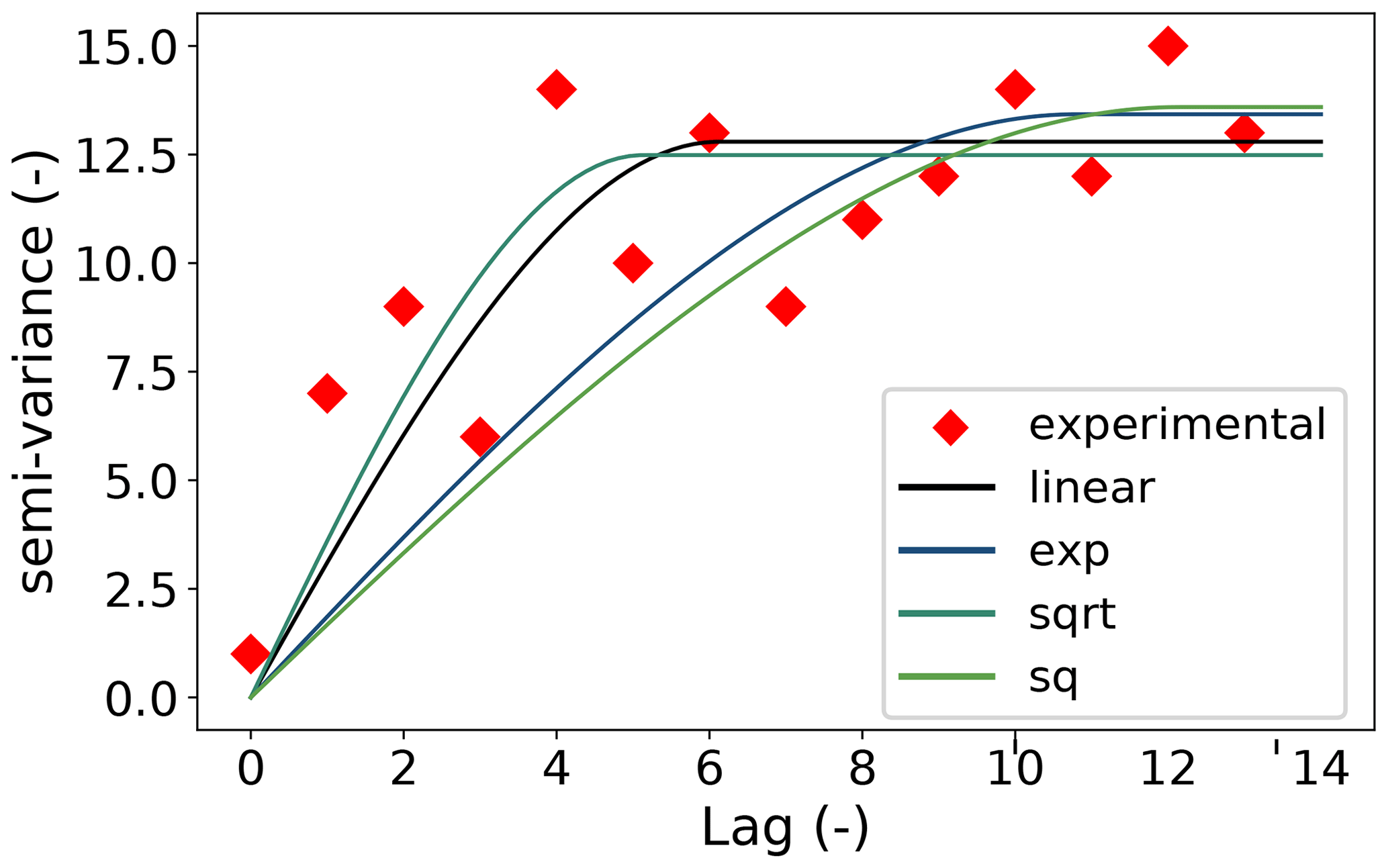
Figure 9Red diamonds show a sample experimental variogram (values are made up) with four different spherical variogram models. All four models are fitted using the trust-region reflective fitting procedure and distance-dependent weights. The weights are linear decreasing with distance (blue line), decreasing by the square root of the normalized distance (green line), the squared normalized distance (red line) and decreasing by exponential function as shown in Eq. (22) (yellow line).
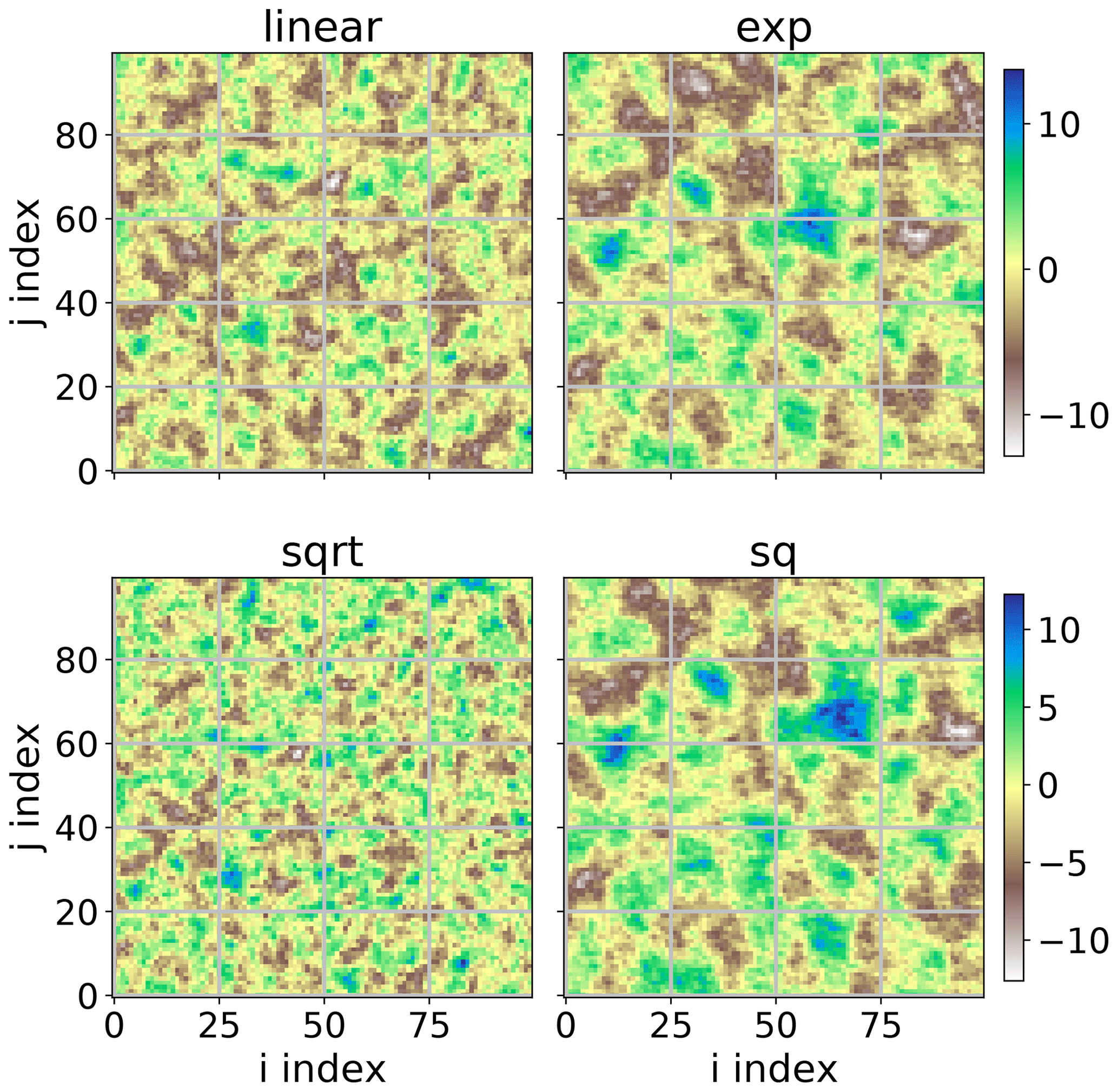
Figure 10Four random fields generated using the same seed for randomization, which results in exactly the same field for same input. The only differing input parameter is the automatic distance-weighting function that was used for fitting the theoretical variogram model. All four fields share the same value range. As the underlying models were made up, neither the values nor the axis coordinates have any meaning. The two coordinate axis names correspond to the index of the random field in matrix form i, j.
Another predefined possibility to determine weights for fitting is information theory. Unlike the other functions, this option is not based on an inverse of weights. The information-theory-based weighting option calculates the uncertainties directly, by using the Shannon entropy (Shannon, 1948). It is calculated for the empirical distribution of point pairs within each distance lag class. This will link the weight during fitting directly to the information content of that lag. From a practical point of view, the resulting weights are usually closer to uniform weights than the distance-dependent weights. For the distance-weighted procedures, the larger lags are almost completely ignored. With the information theory approach, this will only happen for very thinly populated lag classes.
4.1.6 Directional variograms
Directional variograms can be estimated in SciKit-GStat using the DirectionalVariogram class.
It inherits from Variogram, making all its properties and methods available.
Only methods that actually work on the distance matrix are reimplemented to intercept calculations with a spatial filter.
This lets the user interact with the class as learned with the base class, focusing only on the differences between a directional variogram calculation and a classic calculation.
DirectionalVariogram only overwrites one internal method and one property of the base class.
This is the logic assigning the correct lag group to each point pair calculated and then deriving the lag bin edges from this.
In both cases, point pairs are filtered by their orientation, before the calculation is continued.
This way, DirectionalVariogram only adds necessary calculation steps, and the base class does not have to handle data, information or logic (such as point pair orientation) that does not affect the classic calculation.
This conscious design decision leaves the code as readable as possible to make contributions easier for others.
Three new attributes are introduced, which can be set by the user. For all three parameters, SciKit-GStat retains the name, implementation and usage as close to Montero et al. (2015) as possible.
The azimuth of the directional variogram is the direction for which the directional variogram will be calculated. It is given in degrees as a counterclockwise deviation from the coordinate x axis (which will be east in most cases). The tolerance is an angle in degrees, which defines the limit at which a deviation from the azimuth is still acceptable. Only these point pairs will be taken into account, whose orientation as calculated with Eq. (6) is within the tolerance of the azimuth. The tolerance defaults to 45∘.
As the tolerance is given in degrees, the absolute deviations in the unit of the coordinate system can be quite considerable for larger separating distances. Therefore, it is possible to set a bandwidth. This parameter limits the maximum acceptable perpendicular distance from the azimuth vector in coordinate units and defaults to the 33 % percentile of the distance matrix. It can be set as a percentile or as an absolute limit in coordinate units.
Apart from the basic hyper-parameters that define a directional variogram, there are different implementations how to apply them. SciKit-GStat denotes these implementations as directional models and implements two different ones.
The default triangle model is applying the three directional parameters as most often reported in literature (Montero et al., 2015), by constructing a triangle in the direction of the azimuth using the tolerance as an opening window. For larger distances, the triangle is bounded by the bandwidth and turned geometrically into a rectangle.
The unbounded version of the triangle model is called compass, which simply ignores the bandwidth parameter. Thus, it will only restrict point pairs to be oriented into a specific direction.
For convenience and to further inspect the point pairs which are actually taken into account, there is an additional auxiliary plotting method. This plots a network graph for all input locations with an edge for each point pair that will be taken into account for calculation (Fig. 11). Unlike other network graphs, the vertices keep their real locations in the coordinate space to identify specific input data points. A plot like this can be helpful to specify reasonable azimuth and tolerance values, which will highly impact the result.
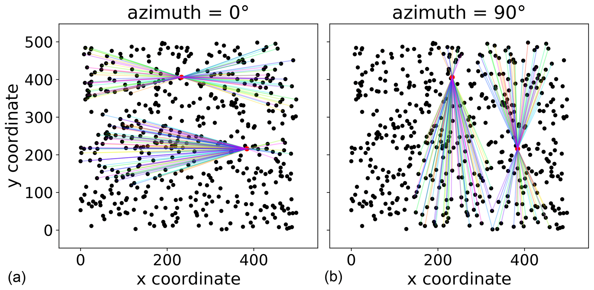
Figure 11Pair Field plot of two directional variograms. The plot was created with exactly the same two directional variogram instances as used in Fig. 5. Panels (a) and (b) show the network graph for two observation points (index 42 and 170 in the sample file), in both directions of the variogram. The lines connect all point pairs that were taken into account for these two points. The line colors have no meaning and are just included for visual reasons.
4.1.7 Spatiotemporal variogram
For calculating spatiotemporal variograms, SciKit-GStat has a class called SpaceTimeVariogram.
Other than the DirectionalVariogram class, SpaceTimeVariogram does not inherit from Variogram but is an independent class.
For a spatiotemporal variogram, any processing step is dependent on not only a spatial lag but also a temporal lag.
This actually changes the function signatures for almost all methods; thus, it was decided to reimplement the whole class without any inheritance.
Nevertheless, SpaceTimeVariogram and Variogram share attribute and method names wherever possible.
At the core of all implemented theoretical variogram methods for the spatiotemporal variogram is the estimation of two marginal variograms.
The class will estimate a temporal and a spatial marginal variogram.
These are both instances of the Variogram class.
The spatiotemporal models themselves expect both marginal variograms as an attribute.
Finally, the SpaceTimeVariogram implements a rich plotting method.
It can plot the experimental spatiotemporal variogram and the
fitted theoretical model as a 3D or 2D plot (Figs. 6 and 7).
For 2D plotting, different plot types are implemented, i.e., a contour plot for semi-variance values.
Both 2D and 3D plots are available. 3D plots allow the user to interactively rotate, pan and zoom the plot, enabling the user to inspect a spatiotemporal variogram. 2D plots are helpful for printed material.
4.1.8 Sub-module: stmodels
SciKit-GStat implements three different theoretical spatiotemporal variogram models: the sum, product and sum-product model.
In line with the models sub-module, the stmodels sub-module has a decorator functions to wrap the models.
This decorator takes care of the data flow and leaves the implementation of the mathematical formula to the user if custom models should be used.
In the following equations the marginal variograms represented by γx, γt refer only to the spatial lag h or temporal lag t, respectively. They are estimated and modeled as described in Sect. 3.1 using any of the semi-variance estimators from Sect. 4.1.3 and any model described in Sect. 4.1.4.
sum is the implementation of the sum model.
This is the most basic spatiotemporal model, which is a sum of a spatial marginal variogram Vx(h) and a temporal marginal variogram Vt(t) as shown in Eq. (23):
where γx and γt are the semi-variance estimations by the two marginal variograms and are not restricted to a specific semi-variance estimator or theoretical model.
The sum model provides an understanding of the idea and workflow of spatiotemporal models. However, it should not be used for real data in almost all cases. It assumes the covariance field to be isotropic across temporal and spatial dimensions, which is a situation which can be considered rarely true. Moreover, it might not be positive definitive, as required for variogram models (Myers and Journel, 1990; Dimitrakopoulos and Luo, 1994).
product is the implementation of the product model.
The implementation is taken from De Cesare et al. (2002, Eq. 4, p. 207) as shown in Eq. (24):
where Cx is the sill parameter of the spatial marginal variogram γx(h), and Ct is the sill of the temporal marginal variogram γt(t).
product_sum is the implementation of the product-sum model.
The implementation is taken from De Cesare et al. (2002, Eq. 6) as shown in Eq. (25):
Here, k1, k2 and k3 are additional fitting parameters needed for the product-sum model. All three parameters need to be positive and may not be larger than any of the marginal sill parameters Cx and Ct.
4.1.9 Ordinary kriging
SciKit-GStat implements an ordinary kriging algorithm. It is implemented following Montero et al. (2015) and can be used using the class OrdinaryKriging.
The user needs to pass an instance of Variogram as a parameter.
In the majority of other kriging implementations, the procedure accepts the observations and estimates a variogram automatically, sometimes even as an internal processing step.
For SciKit-GStat, the decision was made to focus on variogram estimation.
The kriging class should be seen as an auxiliary class to implement the full typical geostatistical analysis workflow.
The user is encouraged to take a closer look at the variogram, utilizing all the plotting routines and descriptions, before passing it on to the kriging class.
This should have a positive effect on geostatistical applications.
It must be noted that the OrdinaryKriging class is mainly implemented for cross-validating variogram models.
It does not claim to be a high-performance implementation of the kriging algorithm,
nor is it implemented with the flexibility and analysis tools that Variogram has.
The author is also aware that further kriging algorithms exist, and ordinary kriging might not be the most useful one.
Thus, SciKit-GStat is more focused on implementing interfaces for other libraries that include other kriging methods.
Namely, these are gstools and pykrige.
To date, the two aforementioned libraries are aligned to each other; future pykrige iterations will implement gstools co-variograms.
This will leave SciKit-GStat only with the need for a powerful interface to gstools to provide the full power of pykrige to SciKit-GStat users.
The SciKit-GStat Variogram class has an interface function that can instantiate any gstools kriging algorithm from a SciKit-GStat variogram.
More details on SciKit-GStat and gstools and their future coexistence are given in Sect. 4.2.
4.2 SciKit-GStat and gstools
SciKit-GStat has three interfaces for gstools, all three implemented as instance methods of the Variogram class.
The first option is to export the empirical variogram.
This is the combination of the lag class edges with the experimental variogram. The lag class edges can optionally be shifted to the class centers, as this is the notation that gstools uses for empirical variograms.
This interface is useful in the case when one of the many binning functions or semi-variance estimators that is not available in gstools was used.
The second, major, option is to translate the theoretical model into a fitted covariance model instance of gstools, which is their respective base class.
With that in place, one can use the covariance model in conjunction with all the great methods available in gstools.
For the specific case of kriging, a third interface exports the variogram directly into a gstools kriging class instance.
At the time of writing, available kriging algorithms were simple kriging, ordinary kriging, universal or regression kriging, kriging with external drift and kriging the mean (Müller et al., 2021).
Both libraries chose different avenues for how the user may interact with the library.
For gstools, the user defines a covariance model and passes it to one of the rich sets of geostatistical functions, which can be found in gstools.
The user then captures the return value of the function and uses it for further development and analysis.
In SciKit-GStat, as described in this paper, the user rather instantiates one object and mutates it during the analysis.
5.1 User support
Users are supported by a comprehensive documentation that includes API reference, installation instructions, a getting started guide, a detailed user guide and tutorials. The user guide is written with the example of a lecture script. No geostatistical prior knowledge is necessary. Only some limited experience of Python and basic knowledge of univariate statistics is advantageous. Additionally, the user guide includes a number of technical notes that discuss some specialities of SciKit-GStat in great detail.
SciKit-GStat is managed and hosted on GitHub under an MIT License. For technical problems, questions and feature requests, the GitHub issues ticketing system is used. To date, any issues arising have been processed by the author himself. As some of the raised issues discussed fundamental geostatistical principles and basic applications of SciKit-GStat, these closed issues are also a valuable resource for new users to SciKit-GStat as well as geostatistics. The evaluation of these issues was taken into account for compiling the user guide.
To use SciKit-GStat in production environments and also for rapid installation, a Docker image is offered. The Dockerfile is also included in the SciKit-GStat repository ,and therefore, also distributed under an MIT License, enabling users to adapt and utilize it. The associated Docker image includes an interactive Jupyter Notebook environment, which auto-starts the tutorials. These tutorials are also included in the documentation and accompany the descriptions. In classroom situations, each student can easily start with the interactive tutorials, while the teacher can follow the documentation. The student should implement the core functionality of SciKit-GStat themselves to fully understand geostatistical analysis workflows. This knowledge can then be applied to SciKit-GStat, emphasizing the correct application of the package and geostatistics in general. Finally, the student can easily apply the learned techniques to real problems with a production-ready Python package. The overall aim is to teach geostatistics with the given resources at the example of SciKit-GStat rather than narrowing geostatistics down to the application of SciKit-GStat only.
5.2 Contributions
Contributions to SciKit-GStat are managed via GitHub. Generally, anyone can create a private copy of the full source code. Adaptions, enhancements or corrections to the source code of SciKit-GStat can be merged into the official code base via GitHub. With respect to coding style, technical correctness and overall objective of the library, any possible contribution is reviewed by the author or any other maintainer of the package. To further guarantee technical correctness, SciKit-GStat is covered by unit tests, which test all main functionalities in isolated test cases. Due to technical challenges, most plotting routines are not covered by unit tests. Historically, there have been a number of tests, but they require a lot of maintenance and are, to a specific degree, dependent on the host platform. Thus, it can be doubted that this is actually beneficial for the user. Additionally, a few tests in the style of end-to-end (e2e) tests were added to run a full analysis against an expected result. Such e2e tests also assess the performance, measured as test runtime. However, dropping performance does not cause a test failure but can be used by the author and contributors to assess contributions with respect to their influence on performance. It was also decided to not accept any new contributions that decrease test coverage significantly, by adding automatic coverage reports to new contributions. This can be considered important to assure a specific level of technical correctness for SciKit-GStat, especially because the open-source MIT License does not put any warranties in place that the user could rely on.
5.3 Integration into other libraries
The main interface to gstools is already discussed in Sect. 4.2.
SciKit-GStat has an interface to pykrige, which makes it possible to export a Variogram instance as kriging parameters directly into pykrige.
However, as pykrige is fundamentally changing, it is not yet clear if the interface will still work in the future.
Nevertheless, as the code restructuring is finished, the more powerful interface to gstools can be used to interact with pykrige in a more feature-rich, natural and native way.
scikit-learn is the most popular data science and machine learning framework in Python.
Besides that, scikit-learn developed a tool-chain pipeline over the past years that is used way beyond data science.
This enables the user to quickly change isolated parts of large and complex automated analysis workflows.
SciKit-GStat implements an interface to the corresponding class in scikit-learn, which makes variogram analysis available in any workflow.
At the same time, scikit-learn implements a great number of data transformation algorithms as usually used in machine learning.
By adopting the pipeline tool-chain, these preprocessing steps can be used together with SciKit-GStat, as many of them are useful for geostatistical preprocessing as well.
A prime example is trend detection and detrending, which is often necessary in geostatistics.
Most limitations and notes on applications have already been mentioned in the respective sections, along with implementation details. This section is discussing general comments on SciKit-GStat. SciKit-GStat is a toolbox for variogram estimation, equipped with a large number of methods. Most of these methods and settings do not make sense in every situation. SciKit-GStat is generally leaving any assessment of estimated variograms, beyond numerical goodness of fit values, to the user. From this, it is further clarified that SciKit-GStat is a variogram estimation toolbox, which is used for building geostatistical methods or conducting analyses. It is not an analysis framework itself.
This limitation also applies to preprocessing. While geostatistical prerequisites, like the intrinsic hypothesis, are mentioned and further literature is referenced, SciKit-GStat does not contain any diagnostic tool to, for example, check given input data any further than by offering the presented scatterplots in Fig. 3 for visual inspection.
External software needs to be used to test and transform input data. This applies to coordinate transformations as well as observation normalization if required.
For both cases, flexible and powerful Python packages are available (scipy, numpy, scikit-learn).
Hence, I had the impression that anything implemented in SciKit-GStat cannot come close to existing software.
Furthermore, I cannot claim to look over all geoscientific fields in enough detail to be able to offer generic integrity checks and preprocessing for just any kind of input data.
On the other hand, from my personal experience in answering GitHub issues, non-transformed, misused and non-applicable datasets in combination with rather uncommon variogram estimations already lead to some confusion.
As an example, if one uses the stable entropy method to find lag classes, the method tries to assure that all classes are of comparable entropy. As a consequence, using the entropy as a variogram estimator will yield nugget effect models by design.
If not, it is due to a weakness in method and not a statistical feature of the sample.
SciKit-GStat will not stop you from doing so, nor does it stop the user from using this model for external drift kriging, which will solely use the external drift variable for interpolation, then.
One might be under the impression that a sophisticated geostatistical interpolation was performed and that the result is backed by the covariance of observations.
In fact, one only applied a computationally intensive averaging overlaid by a simple linear regression of the external drift term.
It is up to the user to inspect the variogram and be aware of these implications.
Not everything SciKit-GStat calculates is automatically correct beyond technical correctness.
Another general comment concerns spatiotemporal geostatistics.
I want to clearly state here that spatiotemporal variograms cannot be exported to any other Python package, and SciKit-GStat does not include spatiotemporal kriging.
No implementation is planned by the author nor for gstools or pykrige as far as I am aware.
Thus, from what I can say, one has to use the wonderful gstat package and the R programming language or gslib in FORTRAN right now.
Due to the lack of kriging procedures, the spatiotemporal variogram representation of SciKit-GStat falls way behind the base class in terms of functionality and interactivity.
Similar statements can be made for the directional variogram.
While it is as functional, interactive and powerful as the base class, it cannot be exported either.
The original intention was to build a diagnostic variography tool for detecting anisotropy.
It turned out that the current design of the directional variogram is incompatible with the design in gstools and pykrige.
Hence, the user has to detect anisotropy and, in the case of geometric anisotropy, then transform the input data manually.
This can be cumbersome, and gstools might offer the better approach here, if kriging or field generation are the final steps.
With SciKit-GStat, the scientific Python community has gained a flexible, well-documented and well-written package for variogram estimation. SciKit-GStat enables the user to estimate variograms in almost limitless variations in a natural language and efficient manner. Many quality measures and especially plotting routines accompany the library to not only do the hard work but also to help the user understand what was actually done. Such an educational aspect of SciKit-GStat is as important as the technical implementation details. Even the best code can be applied the wrong way to draw incorrect or skewed conclusions. If one does not write the code themselves, this risk might be even higher. With SciKit-GStat the focus is on the variogram. Variograms that are better understood by a user lead to better models, which are beneficial not only in application but also as an educational tool.
Users of SciKit-GStat that relate easier to geoscientific data samples than to pancakes are referred to the tutorial section of SciKit-GStat (Mälicke et al., 2022), which includes a sample variogram and kriging application of the Meuse dataset. This dataset is published along with the R package sp (Pebesma and Bivand, 2005; Bivand et al., 2008) and contains 155 samples of heavy-metal ions (cadmium, copper, lead, zinc) along the river Meuse in the Netherlands. In the tutorial, the lead measurements are used. While the original R package description (Pebesma and Bivand, 2005) is not specifying the coordinate reference system used, I am confident that it is Amersfoort/RD New (EPSG: 28992), which projects the sample locations next to the town Stein in the Netherlands. The sample variogram (Fig. A1) is calculated for 15 lag classes up to the median of all separating distances. The spherical theoretical model is fitted using the trust-region reflective method without a nugget effect. The model is under-estimating the semi-variance for the first two lag classes, which could either hint at a nugget or suggest a different spatial model. This requires a detailed assessment of the dataset in any application. One needs to cross-validate at least a Matérn and a stable model, with and without nugget each, before making any decision. However, for this demonstration the variogram is sufficient.
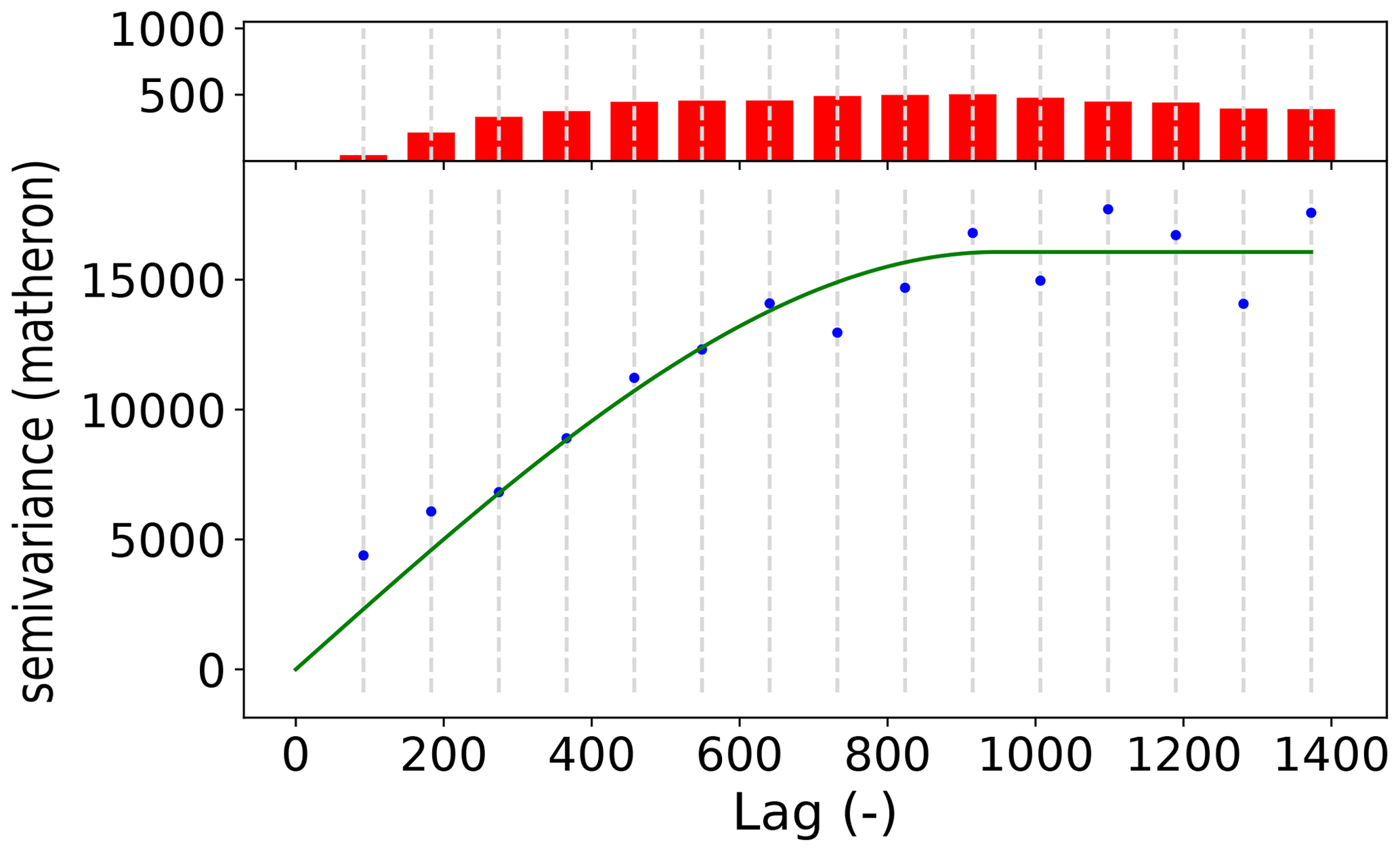
Figure A1Default sample experimental variogram (blue points) with fitted spherical model (green line) of the Meuse dataset (Pebesma and Bivand, 2005; Bivand et al., 2008). The histogram in the upper subplot shows the count of point pairs for each of the 15 lag classes.
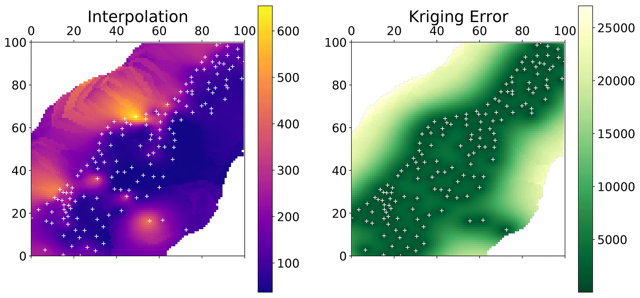
Figure A2Ordinary kriging application using the theoretical variogram model shown in Fig. A1. The kriging procedure estimated the lead concentration on a 100×100 grid.
The model was used to interpolate the sample on a 100×100 sized grid (Fig. A2). This grid size is used to decrease the calculation workload and hardware demand for demonstration purposes only. The grid is bounded by the bounding box of the input coordinates. This results in an irregular cell size of 27.85 m along the x axis and 38.97 m along the y axis. Further, one has to be aware that anything estimated outside of the convex hull of the measurement locations (white points in Fig. A2) is extrapolated and should not be further used.
While this example demonstrates the ease of use of SciKit-GStat, as data sources can simply be exchanged, the application by geostatistics can be way more complicated. SciKit-GStat can help with easily approachable methods and algorithms, but the user still needs expert knowledge to estimate useful variograms and set meaningful hyper-parameters.
Using a photograph of a pancake for geostatistics was fun but not only a joke. When I first saw the browning pattern in the pan, I was just curious if the means of geostatistics work for this example as well. The application was easy and straightforward, and I actually used the first photograph taken. I find it striking how well the variogram estimation worked. I have no other geoscientific real-world or even artificial data example at hand that yielded more textbook-like variograms than this pancake did. Today, I would conclude that while a pancake is not a geoscientific phenomenon, the browning of the dough is largely driven by thermodynamic principles which are universally applicable. Thus, this artificial dataset was great for development and has become my prime benchmark dataset for geostatistical method development. I personally prefer artificial datasets over real-world examples here, as sample sizes and locations can be altered. With real-world datasets I, personally, tend to focus too much on the system that the data actually represents and not the method development. On the other hand, generating a random field by putting a covariance structure represented by a specific variogram into the field and then reproducing the very same variogram from a sample of the field is not much of a surprise. In these use cases, I found pancakes to be very useful.
To bake your own data, there are a few technical instructions that should help to produce comparable pancakes. The photograph was taken with a Canon PowerShot SX540 digital camera at 3267×2305 resolution. The camera position was as orthogonal as possible at about 60 cm height. The original image was rescaled to 709×500 pixels by cubic interpolation and finally cropped to 500×500 pixels, centered along the x axis. To sample the pancake, 300 random pixel positions are chosen, without replacement, to form the array of coordinates. The red-band values at these pixels form the corresponding observations array. The photograph was saved as a PNG file; thus, the value range is of an unsigned 8-bit integer ().
Finally, my pancake dough is very runny (more like a crêpe and less like an American pancake). From my experience, runny dough and high temperatures (short time in the pan) are key to spatially structured pancakes. I would expect a classic American pancake to be way more homogeneously browned. I used 500 g of flour, two medium-sized eggs, about a half liter of milk, a bit of salt and about 50 g of sugar. Finally I added water to the dough until it is about as runny as warm motor oil. Usually, that sums up, at least, to another half liter (of water), maybe a bit more. To bake the random field, use oil not butter. I produced similar results with two different pans on two different stoves (a very old one and a new induction stove). My final advice is to archive only a digital copy of the pancake and eat the actual one with maple syrup.
With version 1.0, SciKit-GStat introduced a utility suite that can generate negative log-likelihood functions for any given Variogram instance.
The definition of a negative log-likelihood function is taken from Lark (2000, Eq. 14).
To construct this function, the utility suite is reading the distance matrix and the theoretical model type from the variogram instance at
runtime and constructs an auto-correlation matrix as defined in Eq. (9) of Lark (2000).
The utility module covers all theoretical functions except the harmonized model, which cannot be fitted.
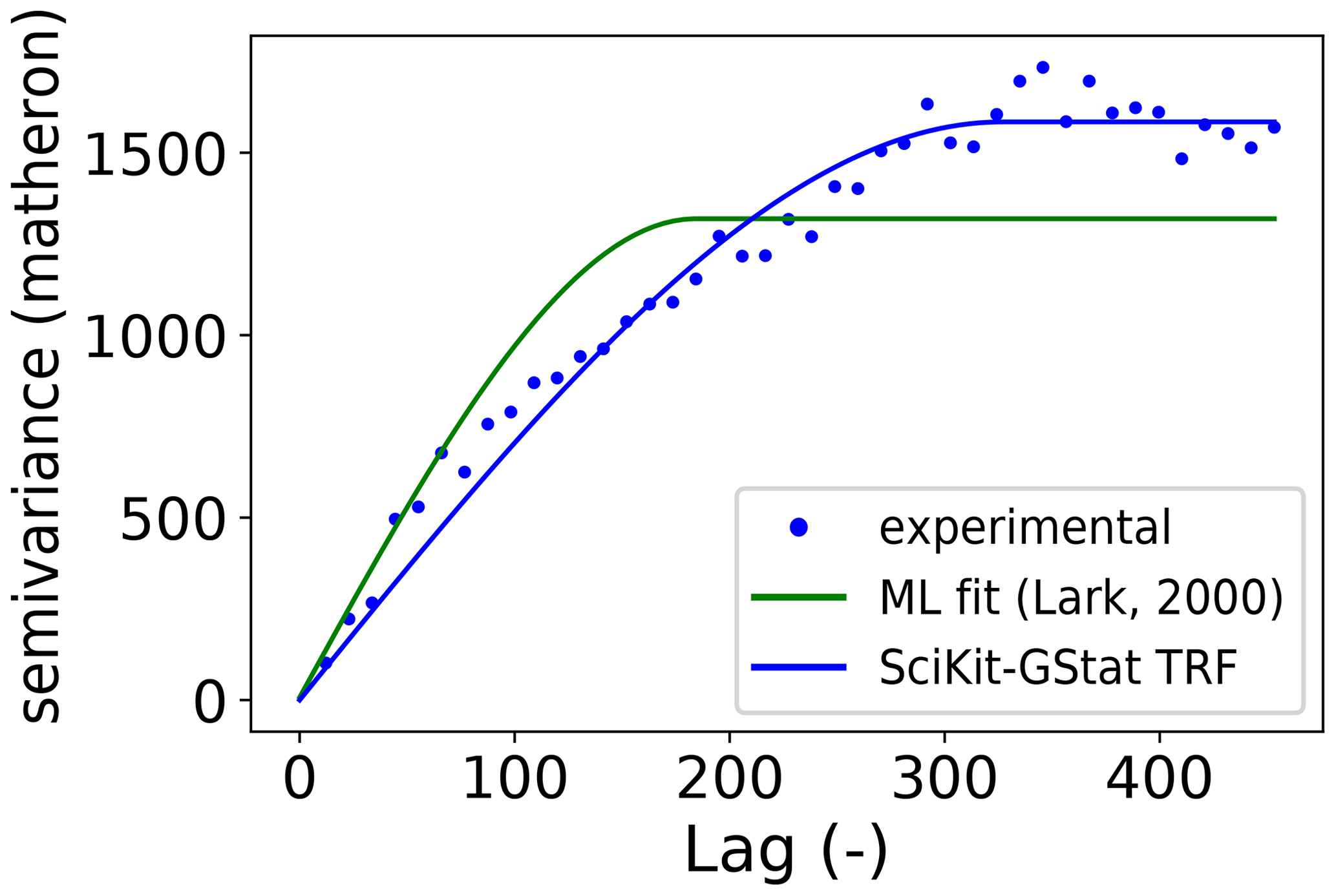
This appendix briefly summarizes the tutorial introducing the utility function. A prime application for using this function is fitting a theoretical variogram model using a maximum likelihood approach (Lark, 2000). SciKit-GStat only returns the likelihood function. It is designed to be used along with SciPy's minimization function (Virtanen et al., 2020) to find optimal variogram parameters by minimizing the negative log-likelihood of the model. The maximum likelihood fit is performed for the pancake sample as well (Fig. C1). For comparison, the default trust-region reflective fit is calculated for the same sample (blue line). In order to highlight a difference between both fits, the binning of the sample used here was changed to Scott's rule (Table 3). While the least-squares fit (blue line) follows the experimental variogram, the maximum likelihood fit does not involve any estimation of an experimental variogram. It covers the first few bins significantly better but at the cost of sample variance, which is underestimated by the maximum likelihood fitted model's sill. From a technical point of view, the maximum likelihood approach should only be used for very small sample sizes. The least squares approaches implemented in SciKit-GStat are by magnitudes faster than minimizing a likelihood function. The computational demand is depending on the auto-correlation matrix for all sample points, which has to be inverted for each evaluation.
The source code of SciKit-GStat is available on GitHub (https://github.com/mmaelicke/scikit-gstat, last access: 21 March 2022). Additionally, each minor version is published as a code publication (https://doi.org/10.5281/zenodo.1345584, Mälicke et al., 2022). The code to reproduce the figures made with SciKit-GStat, including the data samples shown, is available on GitHub and Zenodo (https://doi.org/10.5281/zenodo.5970217, Mälicke, 2021). Note that the data samples are also part of the SciKit-GStat documentation.
All data used in this work are part of SciKit-GStat source code (Mälicke, 2021). The temperature WSN data are derived from Fersch et al. (2020); the Meuse sample was taken with adaptions from the R package sp (Bivand et al., 2008; Pebesma and Bivand, 2005).
The author has declared that there are no competing interests.
Publisher's note: Copernicus Publications remains neutral with regard to jurisdictional claims in published maps and institutional affiliations.
First I want to acknowledge the contributors to SciKit-GStat: Egil Möller, Helge Schneider and Sebastian Müller for their valuable contributions.
I thank Jon Sheppard for proofreading the manuscript and Erwin Zehe for his valuable feedback on general structure, content and data usage.
I also want to emphasize the indirect contributions by Sebastian Müller, the lead developer of gstools.
We spend many hours on discussing the future of Python's geostatistical libraries, which directly affected pykrige, gstools and SciKit-GStat.
Thanks to Sebastian, gstools and SciKit-GStat today complement each other instead of compete with each other.
Finally I thank all the people asking questions and reporting bugs on GitHub.
They made SciKit-GStat a better library and gave me the confidence and the drive to push forward with development, although the paper I wrote the code for in the first place was finished years ago.
The article processing charges for this open-access publication were covered by the Karlsruhe Institute of Technology (KIT).
This paper was edited by Rohitash Chandra and reviewed by three anonymous referees.
Atkinson, P. M. and Tate, N. J.: Spatial Scale Problems and Geostatistical Solutions: A Review, Prof. Geogr., 52, 607–623, https://doi.org/10.1111/0033-0124.00250, 2000. a
Bárdossy, A.: Copula-based geostatistical models for groundwater quality parameters, Water Resour. Res., 42, W11416, https://doi.org/10.1029/2005WR004754, 2006. a
Bárdossy, A. and Lehmann, W.: Spatial distribution of soil moisture in a small catchment. Part 1: Geostatistical analysis, J. Hydrol., 206, 1–15, https://doi.org/10.1016/S0022-1694(97)00152-2, 1998. a, b
Bárdossy, A. and Li, J.: Geostatistical interpolation using copulas, Water Resour. Res., 44, W07412, https://doi.org/10.1029/2007WR006115, 2008. a
Bivand, R. S., Pebesma, E. J., Gómez-Rubio, V., and Pebesma, E. J.: Applied spatial data analysis with R, vol. 747248717, Springer, https://doi.org/10.1007/978-1-4614-7618-4, ISBN 978-1-4614-7617-7, 2008. a, b, c, d
Boisvert, J. B. and Deutsch, C. V.: Programs for kriging and sequential Gaussian simulation with locally varying anisotropy using non-Euclidean distances, Comput. Geosci., 37, 495–510, https://doi.org/10.1016/j.cageo.2010.03.021, 2011. a
Boisvert, J. B., Manchuk, J. G., and Deutsch, C. V.: Kriging in the presence of locally varying anisotropy using non-euclidean distances, Math. Geosci., 41, 585–601, https://doi.org/10.1007/s11004-009-9229-1, 2009. a
Branch, M. A., Coleman, T. F., and Li, Y.: A subspace, interior, and conjugate gradient method for large-scale bound-constrained minimization problems, SIAM J. Sci. Comput., 21, 1–23, 1999. a
Burgess, T. M. and Webster, R.: Optimal interpolation and isarithmic mapping of soil properties. I. The semi-variogram and punctual kriging, J. Soil Sci., 31, 315–331, https://doi.org/10.1111/j.1365-2389.1980.tb02084.x, 1980. a, b, c, d
Chakravarti, N.: Isotonic median regression: a linear programming approach, Math. Oper. Res., 14, 303–308, 1989. a
Christakos, G.: Modern spatiotem poral Geostatistics, 1st edn., Oxford University Press (OUP), New York City, USA, SBN: 0-19-513895-3, 2000. a
Cressie, N. and Hawkins, D. M.: Robust estimation of the variogram: I, J. Int. Ass. Math. Geol., 12, 115–125, https://doi.org/10.1007/BF01035243, 1980. a, b, c
Curriero, F. C.: On the Use of Non-Euclidean Isotropy in Geostatistics on the Use of Non-Euclidean Isotropy in Geostatistics, Johns Hopkins University, Dept. of Biostatistics Working Papers. Working Paper 94, 2005. a
De Cesare, L., Myers, D. E., and Posa, D.: FORTRAN programs for space-time modeling, Comput. Geosci., 28, 205–212, 2002. a, b, c, d, e
Deutsch, C. V. and Journel, A. G.: GSLib, Geostatistical software library and user's guide, Oxford University Press, ISBN 10: 0195073924, 1998. a
Dimitrakopoulos, R. and Luo, X.: Spatiotemporal modelling: covariances and ordinary kriging systems, in: Geostatistics for the next century, Springer, 88–93, https://doi.org/10.1007/978-94-011-0824-9_11, 1994. a
Doane, D. P.: Aesthetic frequency classifications, Am. Stat., 30, 181–183, 1976. a
Dowd, P.: The variogram and kriging: robust and resistant estimators, in: Geostatistics for natural resources characterization, Springer, 91–106, https://doi.org/10.1007/978-94-009-3699-7_6, 1984. a, b
Dowd, P. A.: A review of recent developments in geostatistics, Comput. Geosci., 17, 1481–1500, https://doi.org/10.1016/0098-3004(91)90009-3, 1991. a
Fersch, B., Francke, T., Heistermann, M., Schrön, M., Döpper, V., Jakobi, J., Baroni, G., Blume, T., Bogena, H., Budach, C., Gränzig, T., Förster, M., Güntner, A., Hendricks Franssen, H.-J., Kasner, M., Köhli, M., Kleinschmit, B., Kunstmann, H., Patil, A., Rasche, D., Scheiffele, L., Schmidt, U., Szulc-Seyfried, S., Weimar, J., Zacharias, S., Zreda, M., Heber, B., Kiese, R., Mares, V., Mollenhauer, H., Völksch, I., and Oswald, S.: A dense network of cosmic-ray neutron sensors for soil moisture observation in a highly instrumented pre-Alpine headwater catchment in Germany, Earth Syst. Sci. Data, 12, 2289–2309, https://doi.org/10.5194/essd-12-2289-2020, 2020. a, b, c, d
Freedman, D. and Diaconis, P.: On the histogram as a density estimator: L 2 theory, Z. Wahrscheinlichkeit., 57, 453–476, 1981. a
Gao, F. and Han, L.: Implementing the Nelder-Mead simplex algorithm with adaptive parameters, Comput. Optim. Appl., 51, 259–277, 2012. a, b
Genton, M. G.: Highly robust variogram estimation, Math. Geol., 30, 213–221, 1998. a, b
Goovaerts, P.: Geostatistical approaches for incorporating elevation into the spatial interpolation of rainfall, J. Hydrol., 228, 113–129, 2000. a
Gräler, B., Pebesma, E., and Heuvelink, G.: Spatio-Temporal Interpolation using gstat, R J., 8, 204–218, https://journal.r-project.org/archive/2016/RJ-2016-014/index.html, 2016. a
Guadagnini, A., Riva, M., and Neuman, S. P.: Recent advances in scalable non-Gaussian geostatistics: The generalized sub-Gaussian model, J. Hydro., 562, 685–691, https://doi.org/10.1016/j.jhydrol.2018.05.001, 2018. a
Harris, C. R., Millman, K. J., van der Walt, S. J., Gommers, R., Virtanen, P., Cournapeau, D., Wieser, E., Taylor, J., Berg, S., Smith, N. J., Kern, R., Picus, M., Hoyer, S., van Kerkwijk, M. H., Brett, M., Haldane, A., Del Río, J. F., Wiebe, M., Peterson, P., Gérard-Marchant, P., Sheppard, K., Reddy, T., Weckesser, W., Abbasi, H., Gohlke, C., and Oliphant, T. E.: Array programming with NumPy, Nature, 585, 357–362, https://doi.org/10.1038/s41586-020-2649-2, 2020. a
Hinterding, A.: Entwicklung hybrider Iinterpolationsverfahren für den automatisierten betrieb am beispiel meteorologischer grössen, PhD thesis, Institut für Geoinformatik, Universität Münster, Münster, Germany, 2003. a
Hu, L. Y. and Chugunova, T.: Multiple-point geostatistics for modeling subsurface heterogeneity: A comprehensive review, Water Resour. Res., 44, W11413, https://doi.org/10.1029/2008WR006993, 2008. a
Hunter, J. D.: Matplotlib: A 2D Graphics Environment, Comput. Sci. Eng., 9, 90–95, https://doi.org/10.1109/MCSE.2007.55, 2007. a
Plotly Technologies Inc.: Collaborative data science, https://plot.ly (last access: 21 March 2022), 2015. a
Jewell, S. A. and Gaussiat, N.: An assessment of kriging-based rain-gauge–radar merging techniques, Q. J. Roy. Meteor. Soc., 141, 2300–2313, 2015. a
Johnson, S. C.: Hierarchical clustering schemes, Psychometrika, 32, 241–254, 1967. a
Journel, A. G. and Huijbregts, C. J.: Mining geostatistics, New York, Academic Press, ISBN 1930665911, 1976. a, b, c, d
Kiese, R., Fersch, B., Baessler, C., Brosy, C., Butterbach-Bahl, K., Chwala, C., Dannenmann, M., Fu, J., Gasche, R., Grote, R., Jahn, C., Klatt, J., Kunstmann, H., Mauder, M., Rödiger, T., Smiatek, G., Soltani, M., Steinbrecher, R., Völksch, I., Werhahn, J., Wolf, B., Zeeman, M., and Schmid, H. P.: The TERENO Pre-Alpine Observatory: Integrating meteorological, hydrological, and biogeochemical measurements and modeling, Vadose Zone J., 17, 1–17, 2018. a
Kraft, D.: A software package for sequential quadratic programming, DFVLR-FB 88-28, Koln, Germany, 1988. a
Krige, D. G.: A statistical approach to some basic mine valuation problems on the Witwatersrand, Journal of the chemical metallurgical & mining society of South Africa 52, 119–139, 1951. a
Lark, R.: Estimating variograms of soil properties by the method-of-moments and maximum likelihood, Eur. J. Soil Sci., 51, 717–728, 2000. a, b, c, d, e, f
Ly, S., Charles, C., and Degré, A.: Different methods for spatial interpolation of rainfall data for operational hydrology and hydrological modeling at watershed scale: a review, Biotechnol. Agron. Soc., 17, 1–10, 2015. a
Ma, C.: Spatio-temporal covariance functions generated by mixtures, Math. Geol., 34, 965–975, 2002. a
Ma, C.: Spatio-temporal variograms and covariance models, Adv. Appl. Probab., 725, 706–725, 2005. a
MacQueen, J.: Some methods for classification and analysis of multivariate observations, in: Proceedings of the fifth Berkeley symposium on mathematical statistics and probability, vol. 1, Oakland, CA, USA, 281–297, 1967. a
Mälicke, M.: KIT-HYD/Companion code for SciKit-GStat (10.5194/gmd-2021-174) (0.2.0), Zenodo [code], https://doi.org/10.5281/zenodo.5970217, 2022. a, b
Mälicke, M., Hassler, S. K., Blume, T., Weiler, M., and Zehe, E.: Soil moisture: variable in space but redundant in time, Hydrol. Earth Syst. Sci., 24, 2633–2653, https://doi.org/10.5194/hess-24-2633-2020, 2020. a
Mälicke, M., Hugonnet, R., Schneider, H. D., Müller, S., Möller, E., and Van de Wauw, J.: mmaelicke/scikit-gstat: A scipy flavoured geostatistical variogram analysis toolbox (v1.0.0), Zenodo [code], https://doi.org/10.5281/zenodo.5970098, 2022. a, b, c, d, e, f
Marshall, J., Langille, R., and Palmer, W. M. K.: Measurement of rainfall by radar, J. Meteorol., 4, 186–192, 1947. a
Matheron, G.: Principles of geostatistics, Econ. Geol., 58, 1246–1266, 1963. a, b, c, d
Montero, J.-M., Fernández-Avilés, G., and Mateu, J.: Spatial and spatio-temporal geostatistical modeling and kriging, John Wiley & Sons, ISBN: 978-1-118-41318-0, 2015. a, b, c, d, e, f, g, h, i, j, k, l
Moré, J. J.: The Levenberg-Marquardt algorithm: implementation and theory, in: Numerical analysis, Springer, 105–116, 1978. a
Müller, S., Schüler, L., Zech, A., and Heße, F.: GSTools v1.3: A toolbox for geostatistical modelling in Python, Geosci. Model Dev. Discuss. [preprint], https://doi.org/10.5194/gmd-2021-301, in review, 2021. a, b
Murphy, B., Yurchak, R., and Müller, S.: GeoStat-Framework/PyKrige: v1.6.0, Zenodo, https://doi.org/10.5281/zenodo.4661732, 2021. a
Myers, D. E. and Journel, A.: Variograms with zonal anisotropies and noninvertible kriging systems, Math. Geol., 22, 779–785, 1990. a
Pebesma, E. and Bivand, R. S.: S classes and methods for spatial data: the sp package, R News, 5, 9–13, 2005. a, b, c, d, e
Pebesma, E. J.: Multivariable geostatistics in S: the gstat package, Comput. Geosci., 30, 683–691, 2004. a
Pedregosa, F., Varoquaux, G., Gramfort, A., Michel, V., Thirion, B., Grisel, O., Blondel, M., Prettenhofer, P., Weiss, R., Dubourg, V., Vanderplas, J., Passos, A., Cournapeau, D., Brucher, M., Perrot, M., and Duchesnay, E.: Scikit-learn: Machine Learning in Python, J. Mach. Learn. Res., 12, 2825–2830, 2011. a, b, c, d, e, f, g
Scott, D. W.: Sturges' rule, WIREs Computational Statistics, 1, 303–306, https://doi.org/10.1002/wics.35, 2009. a
Scott, D. W.: Scott's rule, WIREs Computational Statistics, 2, 497–502, https://doi.org/10.1002/wics.103, 2010. a
Shannon, C. E.: A mathematical theory of communication, Bell Syst. Tech. J., 27, 379–423, 1948. a, b, c, d
Thiesen, S., Vieira, D. M., Mälicke, M., Loritz, R., Wellmann, J. F., and Ehret, U.: Histogram via entropy reduction (HER): an information-theoretic alternative for geostatistics, Hydrol. Earth Syst. Sci., 24, 4523–4540, https://doi.org/10.5194/hess-24-4523-2020, 2020. a
van der Walt, S., Colbert, S. C., and Varoquaux, G.: The NumPy Array: A Structure for Efficient Numerical Computation, Comput. Sci. Eng., 13, 22–30, https://doi.org/10.1109/MCSE.2011.37, 2011. a, b, c
Vanderlinden, K., Vereecken, H., Hardelauf, H., Herbst, M., Martínez, G., Cosh, M. H., and Pachepsky, Y. A.: Temporal stability of soil water contents: A review of data and analyses, Vadose Zone J., 11, vzj2011–0178, 2012. a
Vereecken, H., Huisman, J., Bogena, H., Vanderborght, J., Vrugt, J., and Hopmans, J.: On the value of soil moisture measurements in vadose zone hydrology: A review, Water Resour. Res., 44, W00D06, https://doi.org/10.1029/2008WR006829, 2008. a
Virtanen, P., Gommers, R., Oliphant, T. E., Haberland, M., Reddy, T., Cournapeau, D., Burovski, E., Peterson, P., Weckesser, W., Bright, J., van der Walt, S. J., Brett, M., Wilson, J., Millman, K. J., Mayorov, N., Nelson, A. R. J., Jones, E., Kern, R., Larson, E., Carey, C. J., Polat, İ., Feng, Y., Moore, E. W., VanderPlas, J., Laxalde, D., Perktold, J., Cimrman, R., Henriksen, I., Quintero, E. A., Harris, C. R., Archibald, A. M., Ribeiro, A. H., Pedregosa, F., van Mulbregt, P., and SciPy 1.0 Contributors: SciPy 1.0: Fundamental Algorithms for Scientific Computing in Python, Nat. Methods, 17, 261–272, https://doi.org/10.1038/s41592-019-0686-2, 2020. a, b, c, d, e, f, g, h, i, j, k, l
Wackernagel, H.: Anisotropy, Springer, Berlin, Heidelberg, 60–63, https://doi.org/10.1007/978-3-662-03550-4_9, 1998. a, b
Ward Jr., J. H. and Hook, M. E.: Application of an hierarchical grouping procedure to a problem of grouping profiles, Educ. Psychol. Meas., 23, 69–81, 1963. a
Western, A. W., Zhou, S.-L., Grayson, R. B., McMahon, T. A., Blöschl, G., and Wilson, D. J.: Spatial correlation of soil moisture in small catchments and its relationship to dominant spatial hydrological processes, J. Hydrol., 286, 113–134, 2004. a
Zimmermann, B., Zehe, E., Hartmann, N. K., and Elsenbeer, H.: Analyzing spatial data: An assessment of assumptions, new methods, and uncertainty using soil hydraulic data, Water Resour. Res., 44, 1–18, https://doi.org/10.1029/2007WR006604, 2008. a, b
At the time, several undocumented issues arose and solving them was not straightforward.
Note that I only used a measurement every 1.5 h and did not aggregate the time series.
SciKit-GStat is also available on conda-forge, the largest community-driven Anaconda channel. This package is not covered here, as the content is the same and installation requires the presence of an Anaconda environment and some knowledge of the system. Nevertheless, Anaconda is widely spread among scientists, and it might be worth mentioning the existence for Anaconda users.
This only tests the estimation of the experimental variogram and does not test any other functionality. That is, kriging implementations in gstools are substantially faster than in SciKit-GStat. The test was not performed in an isolated environment but repeated several times.
- Abstract
- Introduction
- SciKit-GStat general overview
- Main geostatistical components
- Software implementation
- Support, application and contribution
- Discussion
- Conclusions
- Appendix A: Meuse data
- Appendix B: Pancake data
- Appendix C: Maximum likelihood fitting
- Code availability
- Data availability
- Competing interests
- Disclaimer
- Acknowledgements
- Financial support
- Review statement
- References