Geometric remapping of particle distributions in the Discrete Element Model for Sea Ice (DEMSI v0.0)

A new sea ice dynamical core, the Discrete Element Model for Sea Ice (DEMSI), is under development for use in coupled Earth system models. DEMSI is based on the discrete element method, which models collections of ice floes as interacting Lagrangian particles. In basin-scale sea ice simulations the Lagrangian motion results in significant convergence and ridging, which requires periodic remapping of sea ice variables from a deformed particle configuration back to an undeformed initial distribution. At the resolution required for Earth system models we cannot resolve individual sea ice floes, so we adopt the sub-grid-scale thickness distribution used in continuum sea ice models. This choice leads to a series of hierarchical tracers depending on ice fractional area or concentration that must be remapped consistently. The circular discrete elements employed in DEMSI help improve the computational efficiency at the cost of increased complexity in the effective element area definitions for sea ice cover that are required for the accurate enforcement of conservation. An additional challenge is the accurate remapping of element values along the ice edge, the location of which varies due to the Lagrangian motion of the particles. In this paper we describe a particle-to-particle remapping approach based on well-established geometric remapping ideas that enforces conservation, bounds preservation, and compatibility between associated tracer quantities, while also robustly managing remapping at the ice edge. One element of the remapping algorithm is a novel optimization-based flux correction that enforces concentration bounds in the case of nonuniform motion. We demonstrate the accuracy and utility of the algorithm in a series of numerical test cases.

1 Introduction

Sea ice, the frozen surface of the ocean at high latitudes, forms an important component of the Earth climate system. Sea ice moderates the exchange of heat, mass, and momentum between the ocean and the atmosphere. The high albedo of sea ice has a significant effect on planetary reflectivity and can help drive the polar amplification of climate change through an albedo feedback mechanism (Ingram et al., 1989), while the rejection of salt during sea ice formation helps drive the thermohaline circulation (Killworth, 1983). The sea ice components of current global climate models use a continuum Eulerian formulation and use either structured grids (e.g., CICE: Hunke et al., 2015, or LIM3: Rousset et al., 2015) or unstructured meshes (e.g., MPAS-Seaice: Petersen et al., 2019). Continuum Lagrangian sea ice models have also been developed, such as neXtSIM (Rampal et al., 2016), which uses a moving triangulation as its mesh. The discrete element method (DEM) is an alternate Lagrangian method whereby the motion and contacts of finite-sized particles are simulated. Several DEM sea ice models have been developed for process-scale simulations, such as for sea ice ridging and deformation (Hopkins, 1994), the interaction between sea ice and solid structures (e.g., Tuhkuri and Polojärvi, 2018), the interaction between sea ice and waves (e.g., Xu et al., 2012; Herman, 2017), floe clustering (Herman, 2011), and channel flow (e.g., Gutfraind and Savage, 1998). Basin-scale DEM sea ice models have been developed as well (Hopkins, 2004) and have been used to study the formation of the floe size distribution through fracture processes between elements (Hopkins and Thorndike, 2006).

Ice convergence and ridging present a unique set of issues for sea ice DEM models that are not present in traditional DEM applications. During ridging ice area is reduced as ice thickness increases. Capturing the relevant physics of this process using DEM sea ice models has proven to be a challenge. Hopkins (1994) developed a two-dimensional cross-sectional model of a single pressure ridge, which was used by Hopkins (1996) to derive a contact model for a two-dimensional DEM sea ice model representing the plastic deformation produced during ridge formation. This model was then used to derive sea ice yield curves. Hopkins (2004) used the same contact model in sea ice simulations in which the ridging process was represented through a remapping scheme of overlapping converging neighboring elements. In this model, every 24 h the spatial distribution of elements is remapped back to the initial distribution of elements. Elements that overlap thicken after remapping, representing the ridging process. Without this remapping, element overlap would increase indefinitely, producing a highly interpenetrated element distribution for which determination of element contacts would be difficult, as would interpretation of the sea ice state at any particular point. Alternatively, instead of using overlapped elements to represent ridging, elements could be made to shrink instead. Elements with arbitrarily small radii, however, introduce computational challenges with regard to efficient contact searching, time step size, and contact model formulation (Hopkins, 2004; Shire et al., 2020). Both these considerations therefore require long-duration DEM simulations of sea ice deformation to periodically perform a remapping of the model elements to an undeformed distribution. A related recent development is the non-smooth DEM (NDEM) sea ice model developed by van den Berg et al. (2018, 2019), which for floes of any shape reproduces realistic forces for compliant floe–floe interactions.

Computational performance is another important consideration for long-duration DEM sea ice simulations. One of the most computationally expensive parts of a DEM model is the detection of contact between neighboring elements. Hopkins (2004) use polygonal elements and so require a computationally expensive algorithm (Preparata and Shamos, 1985) to detect contact between elements and to calculate the contact point. Contact detection between circular elements, on the other hand, is much less computationally expensive since for circular elements only a comparison between the element separation and the element radii is needed to determine if elements are in contact. In this regard, in the work which follows, we explore how to represent sea ice in a Hopkins (2004) type of DEM model using more computationally efficient circular elements. Within this framework, we also investigate how to perform proper remapping of elements, which is necessitated by the ridging process and required for the successful development of a global DEM sea ice model performing long-duration simulations.

Considerable research has gone into developing conservative and bounds-preserving remapping methods for transferring scalar quantities between two grids. In the geometric approach, a reconstruction of the conserved quantity is integrated over intersections of overlapping cells between the source and target mesh. In the climate modeling community this class of algorithm has been specialized for remapping between structured and unstructured spherical grids (Jones, 1999; Ullrich et al., 2009). Similar remapping algorithms have been developed for use in arbitrary Lagrangian–Eulerian methods (Margolin and Shashkov, 2003) as well as the remapping step of semi-Lagrangian or incremental remapping schemes for transport (Dukowicz and Baumgardner, 2000; Lipscomb and Hunke, 2001; Lipscomb and Ringler, 2005; Lauritzen et al., 2010). For second-order and higher remapping schemes, a form of limiting must be done to preserve physical bounds on the remapped field. Bounds preservation can be achieved through limiting the gradient of the reconstruction (Dukowicz and Baumgardner, 2000; van Leer, 1979), applying a flux correction algorithm (Liska et al., 2010), or applying an optimization-based correction (Bochev et al., 2013, 2014).

In this paper we present a remapping method that builds on standard geometric remapping approaches while addressing the unique challenges associated with remapping for a DEM sea ice model using circular elements. These challenges include defining consistent areas for enforcing conservation, addressing monotonicity errors due to element overlap under nonuniform motion, and enabling accurate reconstructions at the ice edge. This remapping method forms part of a new sea ice dynamical core, the Discrete Element Model for Sea Ice (DEMSI), currently under development for use in coupled Earth system models. The test cases used here to illustrate the method use a greatly simplified DEM contact model, which is sufficient to demonstrate the efficacy of the remapping method. Work is ongoing to develop a contact model for DEMSI representing sea ice dynamics and including a representation of sea ice fracture and ridging. In Sect. 2 we describe the representation of sea ice in our model and introduce an effective element area needed to represent sea ice with 100 % ice concentration. In Sect. 3 we describe our remapping algorithm including a novel optimization-based flux correction for the case of nonuniform motion and methods for ensuring accurate remap at the ice edge. In Sect. 4 we present numerical examples demonstrating that the method is robust and achieves second-order accuracy, tracer compatibility, conservation, and bounds preservation.

2 Representation of sea ice with circular elements

While using circular elements in DEM models is computationally efficient, they present a unique challenge for the representation of sea ice. Unlike polygonal elements that can be made to completely tessellate a region (e.g., with a Voronoi tessellation), circular elements, in general, cannot completely cover a region, preventing them from directly representing sea ice cover with 100 % concentration. In order to represent 100 % ice cover with circular elements we associate an effective area, e, with each element. This area, which is potentially larger than the geometric area of the circular element, represents the area of sea ice and open water associated with that element. We determine this initial effective element area from a radical Voronoi tessellation (Imai et al., 1985) of the elements. Also called a power or Laguerre–Voronoi diagram, this is a Voronoi tessellation weighted by the element radius and with the element centers as the tessellation generator points. This tessellation results in elements that are contained completely within their polygons for element distributions that do not overlap (see Fig. 1). We take the initial effective area for an element as the area of the radical Voronoi polygon associated with that element. Since the radical Voronoi tessellation covers the whole domain, the effective element area can represent 100 % ice cover. The radical Voronoi polygon associated with an element is carried with it as the element moves.

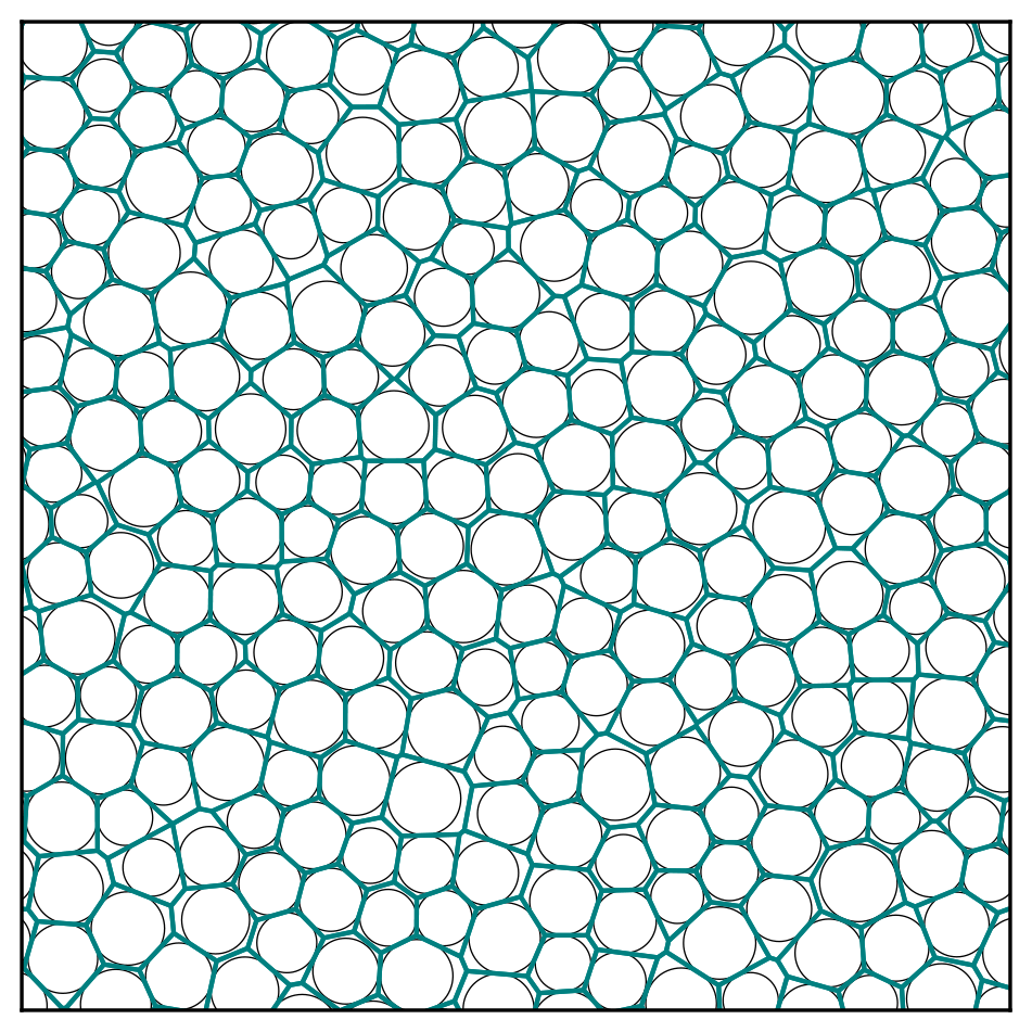
Figure 1 Example of an element distribution generated with the algorithm of Liang et al. (2015) showing the circular elements (grey) and the radical Voronoi tessellation (green).

Over time sea ice deformation and ridging reduce sea ice area (while increasing sea ice thickness and approximately conserving sea ice volume). One way to represent this in a DEM sea ice model is to allow elements to overlap as they ridge and to concomitantly reduce the effective element area as they do. The radical Voronoi polygon associated with an element, P_i, can then be handled in either of two ways. Firstly, the size of the polygon associated with the element, $A_{P_i}$, can be kept constant. In this case $e<A_{P_i}$ in general between remappings. Secondly, as the effective element area of an element decreases during ridging the polygon can be decreased in size so that its area remains equal to the effective element area, i.e., $e=A_{P_i}$, between remappings. The remapping method described here will work with either methodology. We will examine ridging in DEM sea ice models in a later work but require the remapping scheme described here to periodically remap the element distribution back to the initial Voronoi tessellation to ameliorate the effect of the element overlap associated with ridging during long-duration simulations.

Sea ice models used in current global climate models use numerous interdependent tracer fields that form a complex hierarchy with ice concentration, c, or the fractional area of ice in an element, as the root tracer. Sea ice models typically employ an ice thickness category distribution (e.g., Hunke et al., 2015; Rousset et al., 2015), whereby grid cell ice area is divided into a number of categories, each representing sea ice of different thicknesses. The sum of fractional areas in each thickness category is the total element ice concentration. For ice concentration less than 100 %, the remaining area is assumed to be open water. Within each category the ice is further divided into vertical layers, each of which contains tracer fields. Considering both categories and layers, MPAS-Seaice, for example, utilizes 23 different tracer fields for a typical physics simulation without biogeochemistry. Biogeochemistry uses many more additional tracers. Any remapping method must remap this complex tracer hierarchy in a computationally efficient manner and ensure that the sum of ice concentrations across thickness categories per element after remapping is bounded between 0 and 1.

Another desirable property of the remapping scheme is conservation of the appropriate conserved quantities. The effective area, e, provides a means to define conserved quantities that is consistent for a representation of sea ice with 100 % ice concentration. For example, given ice concentration, c, ice thickness, h, and ice enthalpy, q, in element i quantities that must be conserved during remapping are the total ice area per ice thickness category,

$$\begin{array}{}\text{(1)}& {\mathcal{A}}_k=\sum _i{e}_i{c}_{ik},\end{array}$$

the total ice volume per ice thickness category,

$$\begin{array}{}\text{(2)}& {\mathcal{V}}_k=\sum _i{e}_i{c}_{ik}{h}_{ik},\end{array}$$

and the total ice energy per ice thickness category and ice layer,

$$\begin{array}{}\text{(3)}& {\mathcal{Q}}_{kl}=\sum _i{e}_i{c}_{ik}{h}_{ik}{q}_{ikl},\end{array}$$

where each thickness category within an element is labeled by the k index and ice layers within a thickness category by the l index. In the remapping implementation we distinguish between primitive tracer variables, such as thickness and enthalpy, and conserved quantities, such as volume and energy.

3 Geometric remapping implementation

Several properties are desirable in tracer remapping schemes.

• Conservation. A remapping scheme should preserve conservation of the appropriate quantities. Conservation of mass and energy is very important for long-term global climate simulations.

• Accuracy. Since first-order schemes are very numerically diffusive, the method should be at least second-order accurate in space.

• Monotonicity. The method should preserve monotonicity of the tracer fields so no new extrema are generated in these fields by remapping.

• Compatibility. The method should ensure that no new extrema are created when the primitive tracer field is diagnosed from the remapped conserved field; that is, both the primitive and conserved variables are consistently bounds-preserving.

• Computational efficiency. The method should be computationally efficient for many tracers.

The geometrically based remapping scheme proposed here satisfies all these requirements. The method proposed is based partly on the incremental remapping transport algorithm used for sea ice transport in CICE and MPAS-Seaice (Dukowicz and Baumgardner, 2000; Lipscomb and Hunke, 2001). The scheme for remapping a source element distribution (indexed by i) to a destination element distribution (indexed with j) is described below. This remapping method is used within a sea ice simulation to periodically remap a deformed sea ice element (source) distribution to an undeformed (destination) distribution, after which the simulation is restarted. Source element i has its effective area polygon, P_i, advecting with it (including both translation and rotation), while the fixed destination element j has its effective area polygon, P_j, associated with it. Both polygons are convex. The remapping method is based on the polygon, P_ij, associated with the geometric overlap between the P_i and P_j polygons, which is also convex, and consists of transferring quantities associated with P_ij to P_j. Hence, a conserved quantity Z_i on the source polygons is remapped to P_j as

$$\begin{array}{}\text{(4)}& Z_j=\sum _i{Z}_{ij},\end{array}$$

where Z_ij is the part of Z_i in the intersection polygon P_ij and the sum is over the source element polygons, P_i, that overlap the destination polygon, P_j. Since the destination polygons tessellate the whole domain, every part of all the Z_i values, represented in the Z_ij values, is transferred to a destination polygon ensuring conservation of Z.

For a first-order method in which a tracer, t_i, is assumed constant within the P_i polygons,

$$\begin{array}{}\text{(5)}& Z_{ij}=t_i{e}_{ij},\end{array}$$

where e_ij is the effective area associated with the overlap polygon P_ij and is given by the fractional area of the overlap as

$$\begin{array}{}\text{(6)}& e_{ij}=e_i{\displaystyle \frac{A_{P_{ij}}}{A_{P_i}}},\end{array}$$

where $A_{P_i}$ denotes the area of the P_i polygon; recall that e_i is the effective area of element i based on tessellation of the initial element configuration. For a second-order method, with the tracer t_i(x) represented as a linear function of position,

$$\begin{array}{}\text{(7)}& Z_{ij}={\displaystyle \frac{e_{ij}}{A_{P_{ij}}}}\underset{A_{P_{ij}}}{\int }{t}_i\left(\mathit{x}\right)\mathrm{d}A.\end{array}$$

The set of source elements does not necessarily fill the entire domain, as some portions of the domain can be made up of open water. The set of destination polygons, however, forms a complete tessellation of the domain without gaps or overlap, since for conservation every part of the P_i polygons must overlap with a P_j polygon exactly once.

The major steps of the remapping method are described below.

1. Determine overlap polygons, P_ij, between the source (P_i) and destination (P_j) polygons and remap effective element area.

2. Compute linear reconstructions of average tracer fields on source elements based on tracer values in neighboring elements. The gradients in the reconstruction are limited to ensure monotonicity of the remapped fields in the case of uniform motion.

3. Integrate the conserved variables over the intersection polygons using the linear reconstructed tracer fields and aggregate in the destination polygons.

4. Enforce bounds preservation for remapped effective area and tracers using an optimization-based flux correction.

These steps are described in more detail in the following sections.

3.1 Polygon intersections and remapped area

In the first step of the algorithm, the intersection polygons, P_ij, are calculated using the algorithm of Preparata and Shamos (1985). In order to avoid the large computational cost of calculating the intersection polygon for every source and destination polygon pair, only destination polygons that are close enough to source polygons to have potential overlap are included in the search. This is implemented with a link-cell method (Hockney et al., 1974; Plimpton, 1995).

Unlike for the discrete element application described here, when computing intersections between two well-defined grids that cover the same domain, the sum of the intersections will be equal to the domain area. Each destination grid cell will also be entirely covered by source grid cells so that the sum of the source intersections of a destination grid cell will equal the destination grid cell area. For our discrete element application, if the motion leading to the deformed element distribution is nonuniform there may be gaps and overlaps between the source polygons used to compute the intersections. Additionally, near the ice edge there will be destination polygons that are only partially covered by source polygons. To account for this, we compute a remapped effective area, e_j, given by

$$\begin{array}{}\text{(8)}& e_j=\sum _i{e}_{ij}=\sum _i{\displaystyle \frac{A_{P_{ij}}}{A_{P_i}}}{e}_i.\end{array}$$

Recall that e_i may not be equivalent to the effective polygon area associated with element i due to area changes from ridging. The remapped effective area e_j will, in general, not equal the destination element effective area $A_{P_j}$ and in some cases may exceed the destination element effective area. The optimization-based flux algorithm described in Sect. 3.4 is used to correct the remapped effective area to ensure $e_j\le A_{P_j}$ and correct tracer values with the computed area fluxes to enforce monotonicity while maintaining conservation. In the case of uniform motion there are no area changes due to ridging, and the remapped effective area simplifies such that e_i is equal to $A_{P_i}$ and e_j will only differ from $A_{P_j}$ along the ice edge.

3.2 Linear tracer reconstruction

As the first step in remapping the tracers, a mean-preserving linear reconstruction of the tracer fields, t^p(r), is made in each polygon of the source element distribution. For the concentration, c, thickness, h, and enthalpy, q, the reconstructions are

$$\begin{array}{}\text{(9)}& {\displaystyle }& {\displaystyle }{c}^p\left(\mathit{r}\right)=c+{\mathit{\alpha }}_c\mathrm{\nabla }c\cdot (\mathit{r}-\overline{\mathit{r}}),\text{(10)}& {\displaystyle }& {\displaystyle }{h}^p\left(\mathit{r}\right)=h+{\mathit{\alpha }}_h\mathrm{\nabla }h\cdot (\mathit{r}-\stackrel{\mathrm{̃}}{\mathit{r}}),\end{array}$$

and

$$\begin{array}{}\text{(11)}& q^p\left(\mathit{r}\right)=q+{\mathit{\alpha }}_q\mathrm{\nabla }q\cdot (\mathit{r}-\widehat{\mathit{r}}),\end{array}$$

where $\mathit{r}=(x,y)$ is the position vector within the element polygon, ∇c, ∇h, and ∇q are estimates of the tracer gradients for the c, h, and q tracers in the source polygons, and α_c, α_h, and α_q are limiting coefficients for the c, h, and q tracers that enforce monotonicity. A linear tracer reconstruction ensures second-order spatial accuracy of the remapping. To satisfy conservation of 𝒜, 𝒱, and 𝒬, the reconstructed tracer fields must equal the known cell-averaged tracer values (c, h, and q) when integrated over the source polygons so that

$$\begin{array}{}\text{(12)}& {\displaystyle }& {\displaystyle }e{\displaystyle \frac{\mathrm{1}}{A}}\underset{A}{\int }{c}^p\left(\mathit{r}\right)\mathrm{d}A=ce,\text{(13)}& {\displaystyle }& {\displaystyle }e{\displaystyle \frac{\mathrm{1}}{A}}\underset{A}{\int }{c}^p\left(\mathit{r}\right)h^p\left(\mathit{r}\right)\mathrm{d}A=che,\end{array}$$

and

$$\begin{array}{}\text{(14)}& e{\displaystyle \frac{\mathrm{1}}{A}}\underset{A}{\int }{c}^p\left(\mathit{r}\right)h^p\left(\mathit{r}\right)q^p\left(\mathit{r}\right)\mathrm{d}A=chqe.\end{array}$$

This requires that (Lipscomb and Hunke, 2001)

$$\begin{array}{}\text{(15)}& {\displaystyle }& {\displaystyle }\overline{\mathit{r}}={\displaystyle \frac{\mathrm{1}}{A}}\underset{A}{\int }\mathit{r}\mathrm{d}A,\text{(16)}& {\displaystyle }& {\displaystyle }\stackrel{\mathrm{̃}}{\mathit{r}}={\displaystyle \frac{\mathrm{1}}{cA}}\underset{A}{\int }{c}^p\left(\mathit{r}\right)\mathit{r}\mathrm{d}A,\end{array}$$

and

$$\begin{array}{}\text{(17)}& \widehat{\mathit{r}}={\displaystyle \frac{\mathrm{1}}{chA}}\underset{A}{\int }{c}^p\left(\mathit{r}\right)h^p\left(\mathit{r}\right)\mathit{r}\mathrm{d}A.\end{array}$$

Tracer gradients for a source element are calculated as a multivariate linear regression of the tracer values in that element and the neighboring source elements. If two source polygons jointly overlap with a particular destination polygon they are defined as being neighboring source elements. For the n_m neighboring elements (including the element itself) the tracer gradients are given by

$$\begin{array}{}\text{(18)}& {\mathrm{\nabla }}_{x}t={\displaystyle \frac{\left(YY\right)\left(XT\right)-\left(XY\right)\left(YT\right)}{\left(XX\right)\left(YY\right)-(XY{)}^{\mathrm{2}}}}\end{array}$$

and

$$\begin{array}{}\text{(19)}& {\mathrm{\nabla }}_{y}t={\displaystyle \frac{\left(XX\right)\left(YT\right)-\left(XY\right)\left(XT\right)}{\left(XX\right)\left(YY\right)-(XY{)}^{\mathrm{2}}}},\end{array}$$

where

$$\begin{array}{}\text{(20)}& {\displaystyle }& {\displaystyle }XX=\sum _m{x}_m{x}_m-{\displaystyle \frac{\mathrm{1}}{n_m}}\sum _m{x}_m\sum _m{x}_m,\text{(21)}& {\displaystyle }& {\displaystyle }YY=\sum _m{y}_m{y}_m-{\displaystyle \frac{\mathrm{1}}{n_m}}\sum _m{y}_m\sum _m{y}_m,\text{(22)}& {\displaystyle }& {\displaystyle }XY=\sum _m{x}_m{y}_m-{\displaystyle \frac{\mathrm{1}}{n_m}}\sum _m{x}_m\sum _m{y}_m,\text{(23)}& {\displaystyle }& {\displaystyle }XT=\sum _m{x}_m{t}_m-{\displaystyle \frac{\mathrm{1}}{n_m}}\sum _m{x}_m\sum _m{t}_m,\text{(24)}& {\displaystyle }& {\displaystyle }YT=\sum _m{y}_m{t}_m-{\displaystyle \frac{\mathrm{1}}{n_m}}\sum _m{y}_m\sum _m{t}_m.\end{array}$$

Neighboring element m has position (x_m,y_m) and tracer value t_m.

Tracer gradients are limited with a form of van Leer limiting (van Leer, 1979) to preserve monotonicity of the tracer fields. Tracer gradients are limited so that the extrema values of the linear reconstructed tracer field, t_p(r), within a source polygon are within the range of tracer values for the surrounding neighbor source elements. These neighbor elements are defined in the same way as for the gradient calculation above. Since the extremal values of a linear reconstructed tracer field for a polygon are at the corners of that polygon, we use the minimum and maximum of the corner polygon tracer values of the reconstructed field, $t_i^{\text{cmin}}$ and $t_i^{\text{cmax}}$, to perform the limiting. The gradients for a source element i are limited by multiplying them by a limiting coefficient, α_i, which lies in the range [0,1] and whose value is given by

$$\begin{array}{}\text{(25)}& {\mathit{\alpha }}_i=min(\mathrm{1},{\mathit{\alpha }}_{min},{\mathit{\alpha }}_{max}),\end{array}$$

where

$$\begin{array}{}\text{(26)}& {\mathit{\alpha }}_{min}=\left\{\begin{array}{ll}max\left(\mathrm{0},{\displaystyle \frac{t_i^{min}-t_i}{t_i^{\text{cmin}}-t_i}}\right),& \text{if }|t_i^{\text{cmin}}-t_i|>|t_i^{min}-t_i|\\ \mathrm{1},& \text{otherwise}\end{array}\right.\end{array}$$

and

$$\begin{array}{}\text{(27)}& {\mathit{\alpha }}_{max}=\left\{\begin{array}{ll}max\left(\mathrm{0},{\displaystyle \frac{t_i^{max}-t_i}{t_i^{\text{cmax}}-t_i}}\right),& \text{if }|t_i^{\text{cmax}}-t_i|>|t_i^{max}-t_i|\\ \mathrm{1},& \text{otherwise}.\end{array}\right.\end{array}$$

Here, $t_i^{min}$ and $t_i^{max}$ are the minimum and maximum, respectively, of the tracer values of the surrounding neighbor source elements to source element i. This method restricts reconstructed tracer values of a given destination element, t_j, to be within the range of source tracer values for source elements that overlap with the destination element as well as source element neighbors of those source elements, as in the case for the incremental remapping algorithm. In addition, in a similar way gradients of the concentration fields for all the ice thickness categories are limited so that the sum of the reconstructed concentration over thickness categories lies within [0,1].

3.3 Integration over intersection polygons

With tracer gradients calculated and limited, conserved quantities can now be calculated from integrals of the reconstructed tracer fields across the intersection polygons. For destination polygon j,

$$\begin{array}{}\text{(28)}& {\displaystyle }& {\displaystyle }{\mathcal{A}}_{jk}=\sum _i{e}_{ij}{\displaystyle \frac{\mathrm{1}}{A_{P_{ij}}}}\underset{A_{P_{ij}}}{\int }{c}_{ik}^p\left(\mathit{r}\right)\mathrm{d}A,\text{(29)}& {\displaystyle }& {\displaystyle }{\mathcal{V}}_{jk}=\sum _i{e}_{ij}{\displaystyle \frac{\mathrm{1}}{A_{P_{ij}}}}\underset{A_{P_{ij}}}{\int }{c}_{ik}^p\left(\mathit{r}\right)h_{ik}^p\left(\mathit{r}\right)\mathrm{d}A,\end{array}$$

and

$$\begin{array}{}\text{(30)}& {\mathcal{Q}}_{jkl}=\sum _i{e}_{ij}{\displaystyle \frac{\mathrm{1}}{A_{P_{ij}}}}\underset{A_{P_{ij}}}{\int }{c}_{ik}^p\left(\mathit{r}\right)h_{ik}^p\left(\mathit{r}\right)q_{ikl}^p\left(\mathit{r}\right)\mathrm{d}A,\end{array}$$

where the sum is over source element distribution i, and the integral is over the ij intersection polygon area. e_ij is nonzero only when source polygon i overlaps destination polygon j. Finally, new remapped tracer values for the destination elements are determined with

$$\begin{array}{}\text{(31)}& {\displaystyle }& {\displaystyle }{c}_{jk}={\displaystyle \frac{{\mathcal{A}}_{jk}}{e_j}},\text{(32)}& {\displaystyle }& {\displaystyle }{h}_{jk}={\displaystyle \frac{{\mathcal{V}}_{jk}}{e_j{c}_{jk}}},\end{array}$$

and

$$\begin{array}{}\text{(33)}& q_{jkl}={\displaystyle \frac{{\mathcal{Q}}_{jkl}}{e_j{c}_{jk}{h}_{jk}}}.\end{array}$$

Only destination elements with a remapped effective area greater than zero then need to be kept for the continuing DEM simulation. To ensure consistency for partially ice-filled destination elements, before the final calculation of tracer values in Eqs. (31) to (33), the effective area is set to the polygon area $A_{p_j}$, decreasing the concentration of sea ice calculated in Eq. (31). This is compatible with Eq. (8) since the values of effective area and concentration are not unique for representing the physically relevant quantity of sea ice area within an element, given by 𝒜_i=c_ie_i. Provided the area of sea ice within an element remains fixed, $\mathrm{0}\le c_i\le \mathrm{1}$, and $\mathrm{0}\le e_i\le A_p$, the concentration and effective area can vary together without affecting the physical representation.

Instead of directly calculating the integrals over the source and intersection polygon area required by the remapping method, the integrands of these integrals are expanded so that only integrals of geometric quantities of the source polygons are required. These quantities are calculated once for all tracers, improving computational efficiency for simulations with a large tracer number. For example, Eq. (16) once expanded becomes

$$\begin{array}{}\text{(34)}& \begin{array}{rl}{\stackrel{\mathrm{̃}}{\mathit{r}}}_x={\displaystyle \frac{\mathrm{1}}{cA}}[& (c-{\mathit{\alpha }}_c\mathrm{\nabla }c\cdot \overline{\mathit{r}})\underset{A}{\int }x\mathrm{d}A+\left({\mathit{\alpha }}_c{\mathrm{\nabla }}_{x}c\right)\underset{A}{\int }{x}^{\mathrm{2}}\mathrm{d}A\\ & +\left({\mathit{\alpha }}_c{\mathrm{\nabla }}_{y}c\right)\underset{A}{\int }xy\mathrm{d}A]\end{array}\end{array}$$

and

$$\begin{array}{}\text{(35)}& \begin{array}{rl}{\stackrel{\mathrm{̃}}{\mathit{r}}}_y={\displaystyle \frac{\mathrm{1}}{cA}}[& (c-{\mathit{\alpha }}_c\mathrm{\nabla }c\cdot \overline{\mathit{r}})\underset{A}{\int }y\mathrm{d}A+\left({\mathit{\alpha }}_c{\mathrm{\nabla }}_{x}c\right)\underset{A}{\int }xy\mathrm{d}A\\ & +\left({\mathit{\alpha }}_c{\mathrm{\nabla }}_{y}c\right)\underset{A}{\int }{y}^{\mathrm{2}}\mathrm{d}A],\end{array}\end{array}$$

and only source polygon integrals of x, y, x², y², and xy are required. The integrals are calculated by breaking polygons into triangles by connecting the polygon centroid to the polygon vertices and using the Gaussian triangular quadrature rules of Dunavant (1985).

3.4 Optimization-based flux correction to remapping

For uniform motion of the elements there is no relative motion (either rectilinear or rotational) between elements, so their polygons do not overlap during their motion. For general motion, however, relative motion between elements results in element polygons overlapping. For the formulation of effective area from Sect. 2, this would potentially result in the remapped effective area exceeding the available geometric area of the destination polygons, resulting in remapped concentrations greater than 1. To ameliorate this issue we implement a flux-based optimization correction to the effective area and tracer fields that is applied after the remapping discussed above. This optimization scheme determines a minimal flux, $f_{j_{\mathrm{1}}{j}_{\mathrm{2}}}$, between polygons j₁ and j₂ of the destination element distribution that conservatively removes excess effective area from destination polygons, so after the flux is applied to the remapped effective area and tracer fields the effective areas, $e_{j_{\mathrm{1}}}$ and $e_{j_{\mathrm{2}}}$, are less than the destination polygon areas, $A_{P_{j_{\mathrm{1}}}}$ and $A_{P_{j_{\mathrm{2}}}}$, for all destination polygons. For a given destination polygon $P_{j_{\mathrm{1}}}$ we require that the corrected effective area, $e_{j_{\mathrm{1}}}^{\prime }$, obey

$$\begin{array}{}\text{(36)}& \mathrm{0}\le e_{j_{\mathrm{1}}}^{\prime }\le A_{P_{j_{\mathrm{1}}}}.\end{array}$$

The corrected effective area is given by

$$\begin{array}{}\text{(37)}& e_{j_{\mathrm{1}}}^{\prime }=e_{j_{\mathrm{1}}}+\sum _{j_{\mathrm{2}}}{B}_{j_{\mathrm{1}}{j}_{\mathrm{2}}}{f}_{j_{\mathrm{1}}{j}_{\mathrm{2}}},\end{array}$$

where $B_{j_{\mathrm{1}}{j}_{\mathrm{2}}}$ is the j₁,j₂ component of a sparse matrix with entries of either 0 (if polygons j₁ and j₂ do not share an edge), −1, or 1 (signifying whether the flux $f_{j_{\mathrm{1}}{j}_{\mathrm{2}}}$ is into or out of the polygon j₁). Thus, the determination of the set of fluxes, $f_{j_{\mathrm{1}}{j}_{\mathrm{2}}}$, can be cast in the following inequality constrained quadratic program:

$$\begin{array}{}\text{(38)}& \begin{array}{rl}\text{minimize }& {\displaystyle \frac{\mathrm{1}}{\mathrm{2}}}{\mathit{f}}^{\mathrm{T}}\mathbf{P}\mathit{f}\\ \text{subject to }& \mathit{l}\le \mathbf{B}\mathit{f}\le \mathit{u},\end{array}\end{array}$$

where f is the vector of edge fluxes, $f_{i_{\mathrm{1}}{j}_{\mathrm{2}}}$, P is the identity matrix, B is the matrix with components $B_{j_{\mathrm{1}}{j}_{\mathrm{2}}}$, and u and l are vectors defined by

$$\begin{array}{}\text{(39)}& l_j=-e_j\end{array}$$

and

$$\begin{array}{}\text{(40)}& u_j=A_{P_j}-e_j.\end{array}$$

The quadratic program is solved in parallel by the PermonQP library (Hapla et al., 2016; Kružík et al., 2020; Hapla et al., 2021), which uses the PETSc library (Balay et al., 1997, 2019). The fluxes, $f_{j_{\mathrm{1}}{j}_{\mathrm{2}}}$, are then used to conservatively transfer effective area and tracer quantities between destination polygons, removing excess effective area. Since the fluxes are fluxes of effective area, a conserved quantity, Z, is corrected according to

$$\begin{array}{}\text{(41)}& Z_{j_{\mathrm{1}}}^{\prime }=Z_{j_{\mathrm{1}}}-Z_{j_{\mathrm{1}}}{\displaystyle \frac{f_{j_{\mathrm{1}}{j}_{\mathrm{2}}}}{e_j}}\end{array}$$

and

$$\begin{array}{}\text{(42)}& Z_{j_{\mathrm{2}}}^{\prime }=Z_{j_{\mathrm{2}}}+Z_{j_{\mathrm{1}}}{\displaystyle \frac{f_{j_{\mathrm{1}}{j}_{\mathrm{2}}}}{e_j}}\end{array}$$

for all values of f, where $f_{j_{\mathrm{1}}{j}_{\mathrm{2}}}$ flows from element j₁ to j₂.

Another issue ameliorated by the flux correction is the overlapping of source elements with coastal elements. Here we represent coastlines through a series of immovable elements coincident with land. DEM models, however, model compressive interaction through an overlap of elements, so sea ice elements pushed by winds onto fixed coastal elements will overlap slightly with those elements. During the remapping described previously some sea ice will be remapped onto the coastal elements. This can be fixed by moving this remapped ice to the nearest destination element that is not a coastal element before the flux correction is performed. While moving this ice has the potential to increase the effective area of these elements to be larger than their geometric area, the flux correction algorithm ameliorates this effect.

Figure 2 (a) Final ice concentration for the one-dimensional top hat test case. No remapping (solid), low-order remapping, and higher-order (dashed) remapping. (b) As (a) but with a logarithmic ordinate axis. Results for no remapping, low-order remapping, and higher-order remapping are shown.

3.5 Effect of open water

One difference between particle and Eulerian methods that causes potential issues for remapping is the treatment of open water. In Eulerian methods, empty Eulerian cells, representing open water, can be included in the calculation of tracer gradients and monotonicity limits. For DEM sea ice models, elements only exist where sea ice exists, with elements that lose all their ice being removed from the simulation. One advantage of this is that fewer elements are needed than Eulerian cells (which must cover the whole domain), increasing computational performance for the DEM model. Consequently, there are no empty elements representing open water to be included in tracer gradient calculations or in the neighboring element tracer extrema used to limit those gradients. A possible effect of this is that tracer values for ice concentration and thickness, t_i, for elements at the ice pack edge are likely to be the minimum of the neighbor tracer values so that $t_i=t_{ij}^{min}$. From Eqs. (25) to (27) this would mean the gradients would be limited to zero in these ice edge elements, and the remapping here would revert to a highly diffusive first-order method. To investigate the effect of this issue we implement a method to account for open water in the tracer gradient calculation and limiting. Firstly, for the neighboring source elements, N_i, of a given source element (not including the element itself) we calculate the total effective area, E_i, and the centroid of that effective area, ${\mathit{r}}_{E_i}$. These are given by

$$\begin{array}{}\text{(43)}& E_i=\sum _i^{N_i}{e}_i\end{array}$$

and

$$\begin{array}{}\text{(44)}& {\mathit{r}}_{E_i}={\displaystyle \frac{\mathrm{1}}{E}}\sum _i^{N_i}{e}_i{\mathit{r}}_i.\end{array}$$

If the E_i is below some limit we assume that there is some open water surrounding the source element and include an additional open-water neighbor pseudo-element into the gradient and gradient-limiting calculations. This pseudo-element has zero concentration and a position on the opposite side of the element to the centroid of the surrounding effective area ($\mathrm{2}{\mathit{r}}_i-{\mathit{r}}_{E_i}$). The addition of a neighbor concentration value of zero would prevent the gradient at the ice edge from being limited to zero. We include the zero concentration pseudo-element if the sea ice surrounding the element of interest is below a fraction (taken as 0.75) of an estimate of the expected value of E_i for a fully covered pack, $E_i^{\prime }$. In two dimensions we estimate $E_i^{\prime }$ based on a hexagonal close packing of elements so that $E_i^{\prime }\simeq \mathrm{6}{\overline{A}}_{P_j}$, where ${\overline{A}}_{P_j}$ is the mean area of destination polygons. In one dimension each element is only surrounded by two elements, so for one-dimensional tests we use $E_i^{\prime }\simeq \mathrm{2}{\overline{A}}_{P_j}$.

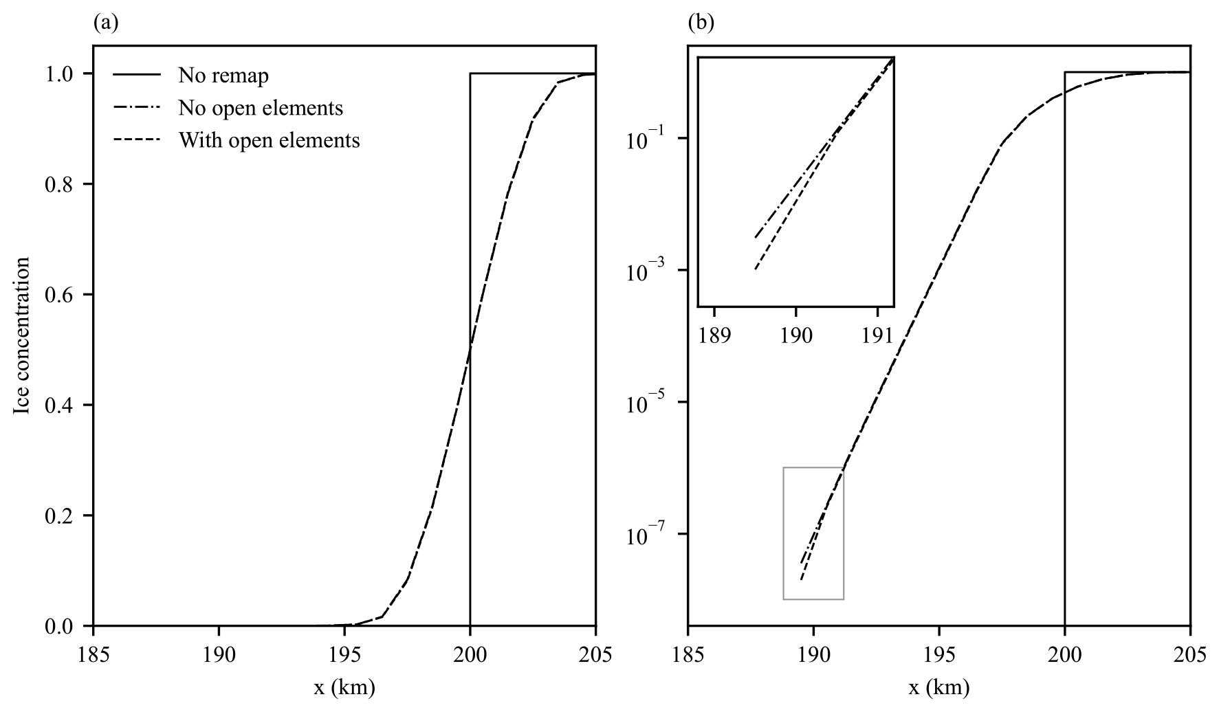
Figure 3 (a) Detail of ice concentration for the top hat test case showing the higher-order remapping results with and without taking into account the effect of open water. (b) As (a) but with a logarithmic ordinate axis. The inset shows detail of the differences at the extreme of the distribution.

4 Computational results

We now test the remapping algorithm described in the previous section with a series of idealized test cases. Motion of the elements between remapping is determined by the LAMMPS (Plimpton, 1995) molecular dynamics code, which has the capability to run DEM simulations, wherein particle interaction forces are computed based on contacts and the equations of motions are integrated in time. LAMMPS can either explicitly enforce the motion of elements (such as in uniform rectilinear motion) or solve the equations of motion of the elements with a modified velocity Verlet integrator (Swope et al., 1982). For test cases involving solving the equations of motion, we solve a simplified sea ice momentum equation, which in a DEM context reduces to a set of coupled first-order equations for all elements:

$$\begin{array}{}\text{(45)}& m_i{\displaystyle \frac{\mathrm{d}{\mathit{u}}_i}{\mathrm{d}t}}=\sum _j{\mathit{F}}_{ij}+{\mathit{\tau }}_{\mathrm{a}}\left({\mathit{x}}_i\right)+{\mathit{\tau }}_{\mathrm{w}}\left({\mathit{x}}_i\right),\end{array}$$

where m_i is the mass of each element, u_i is the element velocity, F_ij is the contact force on element i from neighboring element j, and τ_a and τ_w are the atmospheric and ocean stresses, respectively, evaluated at the location of the element x_i. To determine element rotation we also solve an angular momentum equation given by

$$\begin{array}{}\text{(46)}& I_i{\displaystyle \frac{\mathrm{d}{\mathit{\omega }}_i}{\mathrm{d}t}}=\sum _j({\mathit{r}}_{ij}\times {\mathit{F}}_{ij}),\end{array}$$

where I_i is the moment of inertia of element i, ω_i is the element angular velocity, (r_ij×F_ij) is the torque on element i produced by the contact force with element j, and r_ij is the contact position between elements i and j relative to the center of mass of element i. The surface stresses have a quadratic form given by

$$\begin{array}{}\text{(47)}& \mathit{\tau }=e{c}_{\mathrm{a},\mathrm{w}}{\mathit{\rho }}_{\mathrm{a},\mathrm{w}}|{\mathit{U}}_{\mathrm{a},\mathrm{w}}-\mathit{u}|({\mathit{U}}_{\mathrm{a},\mathrm{w}}-\mathit{u}),\end{array}$$

where e is the effective element area, c_a,w is a drag coefficient, ρ_a,w is the fluid density, U_a,w is the fluid velocity, subscript a refers to air, and subscript w refers to water. This momentum equation is discretized in time as

$$\begin{array}{}\text{(48)}& \begin{array}{rl}m{\displaystyle \frac{{\mathit{u}}^n-{\mathit{u}}^{n-\mathrm{1}}}{\mathrm{\Delta }t}}=& {\mathit{F}}_{n-\mathrm{1}}+e{c}_{\mathrm{a}}{\mathit{\rho }}_{\mathrm{a}}\left|{\mathit{U}}_{\mathrm{a}}-{\mathit{u}}^{n-\mathrm{1}}\right|\left({\mathit{U}}_{\mathrm{a}}-{\mathit{u}}^{n-\mathrm{1}}\right)\\ & +e{c}_{\mathrm{w}}{\mathit{\rho }}_{\mathrm{w}}\left|{\mathit{U}}_{\mathrm{w}}-{\mathit{u}}^{n-\mathrm{1}}\right|\left({\mathit{U}}_{\mathrm{w}}-{\mathit{u}}^n\right),\end{array}\end{array}$$

where superscripts n and n−1 signify the current and previous time steps, respectively, and the ocean velocity is treated partly implicitly for stability. For the test cases considered here a simple Hookean elastic repulsion contact model is employed with velocity damping in both the normal and tangential contact directions. While the Hookean contact model has several limitations, such as sensitivity to the time step and to the time stepping method used, it is sufficient to demonstrate the efficacy of the remapping method. The air drag coefficient, c_a, and air density, ρ_a, are given by 0.0012 and 1.3 kg m⁻³, respectively (Hibler, 1979), while the ocean drag coefficient, c_w, and water density, ρ_w, are given by 0.00536 and 1026 kg m⁻³ (Kim et al., 2006), respectively.

4.1 One-dimensional uniform motion

The first test we perform is a simple one-dimensional test case with uniform motion and a “top hat” initial ice concentration distribution. The destination element distribution consists of uniform elements with radius, r, of 500 m arranged in the x direction across a domain 1000 km long. The domain accommodates a single element in the y direction and is 1 km wide. The initial source distribution is a subset of the destination distribution consisting of the 100 elements between 100 and 200 km in the x direction. Initial ice concentration, c₀(x), is given by

$$\begin{array}{}\text{(49)}& c_{\mathrm{0}}\left(x\right)=\left\{\begin{array}{ll}\mathrm{1},& \text{for }{x}_{\mathrm{1}}\le x\le x_{\mathrm{2}}\\ \mathrm{0},& \text{otherwise},\end{array}\right.\end{array}$$

where x₁ and x₂ are 100 and 200 km, respectively.

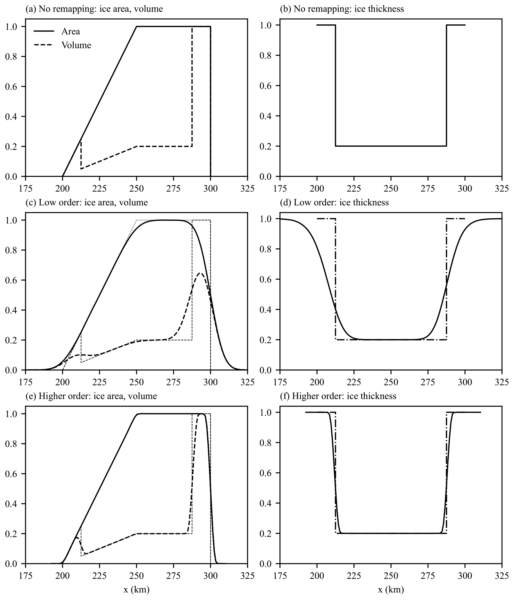
Figure 4 One-dimensional compatibility test case. (a, b) No remapping, (c, d) low-order remapping, (e, f) higher-order remapping. (a, c, e) Ice concentration and volume; (b, d, f) ice thickness.

These elements have an initial effective area of a square of side 2r, a sea ice concentration of 1, and a sea ice thickness of 1 m. The elements undergo uniform motion in the positive x direction for a total of 100 km of translation, whereupon the final source distribution is examined. Figure 2 shows this final distribution for three situations. The first situation (“no remap” in Fig. 2) has no remapping performed during the uniform motion so that the final distribution of ice concentration and thickness is the same as the initial one, other than being translated 100 km in the positive x direction. For the second situation (“low order” in Fig. 2) the source distribution elements move half their diameter (500 m) before remapping and undergo a total of 200 remappings, resulting in the 100 km total translation. Tracer gradients are set to zero so that the remapping algorithm becomes a low-order method. The final situation (“higher order” in Fig. 2) is the same as the low-order situation except tracer gradients are not set to zero, making the remapping a more accurate higher-order method. The no remap situation is useful for demonstrating the final distribution that a perfect remapping scheme, with no numerical diffusion, would produce. Figure 2 shows that the higher-order method produces significantly less numerical diffusion of the concentration profile than the low-order method.

We now use this test case to explore the effect of taking account of open water in the tracer gradient and limiting, as described in Sect. 3.5. We rerun the higher-order simulation with and without the effects of open water taken into account (see Fig. 3). As can be seen in Fig. 3 the effect of the absence of open-water elements appears negligible with only a very minor amount of extra numerical diffusion present at the very edge of the ice due to this absence (see inset in Fig. 3b). Similar results were found with the two-dimensional simulations described next. Based on these results we neglect the effect of the absence of open-water elements for the remainder of this work.

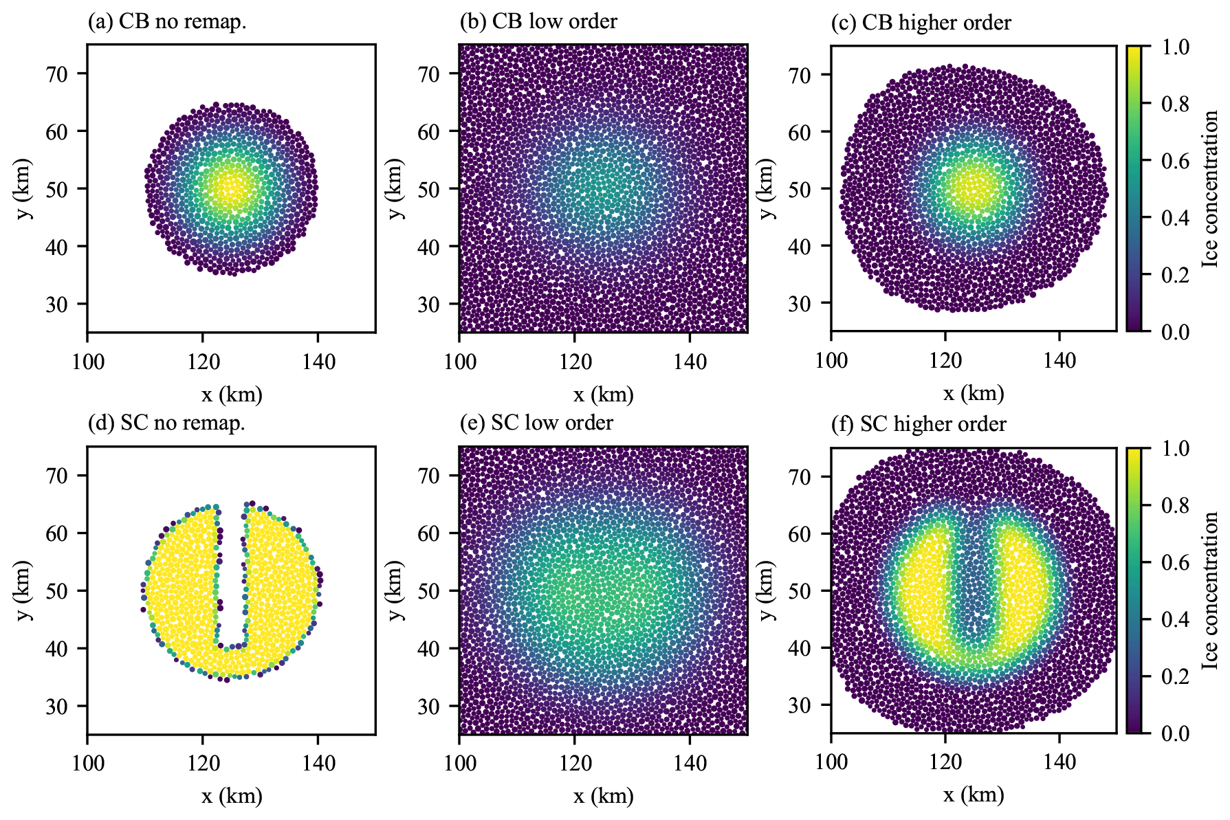
Figure 5 Final ice concentration (fraction of elements covered in sea ice) for the two-dimensional remapping test case with an initial cosine bell (CB: a–c) and slotted cylinder (SC: d–f) particle distribution. (a, d) No remapping, (b, e) low-order remapping, and (c, f) higher-order remapping.

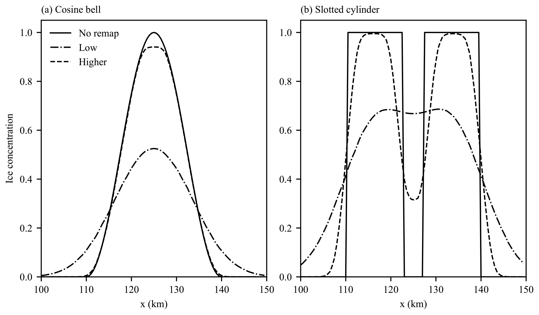
Figure 6 Cross section (y = 50 km) of ice concentration for the two-dimensional test case for the initial (a) cosine bell and (b) slotted cylinder particle distributions. Results for no remapping, low-order remapping, and higher-order remapping are shown.

The next one-dimensional test case is based on that found in Lipscomb and Hunke (2001) and is used to test how well the remapping algorithm preserves the compatibility of the particle tracers. The test case is the same as the previous one-dimensional test case, except for the initial distribution of ice concentration, thickness, and volume. These initial distributions are more complex than the previous test case (see Fig. 4a and b) and provide a harder test of compatibility. Initial ice concentration, c₀(x), and thickness, h₀(x), are given by

$$\begin{array}{}\text{(50)}& c_{\mathrm{0}}\left(x\right)=\left\{\begin{array}{ll}\frac{x-x_{\mathrm{1}}}{x_{\mathrm{3}}-x_{\mathrm{1}}},& \text{for }{x}_{\mathrm{1}}\le x\le x_{\mathrm{3}}\\ \mathrm{1},& \text{for }{x}_{\mathrm{3}}\le x\le x_{\mathrm{5}}\\ \mathrm{0},& \text{otherwise}\end{array}\right.\end{array}$$

and

$$\begin{array}{}\text{(51)}& h_{\mathrm{0}}\left(x\right)=\left\{\begin{array}{ll}\mathrm{0.25},& \text{for }{x}_{\mathrm{2}}\le x\le x_{\mathrm{4}}\\ \mathrm{1},& \text{for }(x_{\mathrm{1}}\le x<x_{\mathrm{2}})\mathbf{or}(x_{\mathrm{4}}<x\le x_{\mathrm{5}}),\end{array}\right.\end{array}$$

where x₁, x₂, x₃, x₄, and x₅ are given by 100, 112.5, 150, 187.5, and 200 km, respectively. As before we perform three separate simulations: one with no remapping (Fig. 4a and b), one with low-order remapping (Fig. 4c and d), and one with higher-order remapping (Fig. 4e and f). As before both the low- and higher-order remapping schemes are capable of remapping the initial particle distribution, with the higher-order scheme producing much less numerical diffusion. Figure 4d and f also clearly show that the thickness tracer preserves monotonicity as well as the concentration and volume, clearly demonstrating compatibility of the method.

4.2 Two-dimensional uniform motion

The next test case we examine involves a two-dimensional domain of size 300 km in the x direction and 100 km size in the y direction. The destination and initial source element distributions consist of a random arrangement of circular elements with a distribution of element radius, with mean radius ∼ 513 m. To create the tightly packed initial element distribution we use the method of Liang et al. (2015). This method uses a Lloyd (1982) type of iteration of the radical Voronoi tessellation of an initial random set of generator points each with an assigned radius drawn from a distribution. During each iteration the generator locations are moved to the centers of the largest inscribed circles within the radical Voronoi polygons (see Fig. 1 for an example element distribution generated with this method). We explore two different initial source element distributions discussed in Lipscomb and Ringler (2005). The first is a cosine bell distribution with an initial ice concentration, c₀(x,y), given by

$$\begin{array}{}\text{(52)}& c_{\mathrm{0}}(x,y)=\left\{\begin{array}{ll}\frac{\mathrm{1}}{\mathrm{2}}\left(\mathrm{1}+\cos \left(\frac{\mathit{\pi }r}{r_{\mathrm{0}}}\right)\right),& r<r_{\mathrm{0}}\\ \mathrm{0},& \text{otherwise},\end{array}\right.\end{array}$$

where $r=\sqrt{(x-x_{\mathrm{0}}{)}^{\mathrm{2}}+(y-x_{\mathrm{0}}{)}^{\mathrm{2}}}$, (x₀,y₀) is the center of the cosine bell at (25 km, 50 km), and r₀ is the radius of the cosine bell with size 15 km. The second is a slotted cylinder with an initial ice concentration, c₀(x,y), given by

$$\begin{array}{}\text{(53)}& c_{\mathrm{0}}(x,y)=\left\{\begin{array}{ll}\mathrm{1},& (r<r_{\mathrm{0}})\mathbf{and}\mathbf{not}\\ & \left(\right(|x-x_{\mathrm{0}}|<\frac{\mathrm{1}}{\mathrm{6}}{r}_{\mathrm{0}}\left)\mathbf{and}\right(y-y_{\mathrm{0}})>-\frac{\mathrm{2}}{\mathrm{3}}{r}_{\mathrm{0}}))\\ \mathrm{0},& \text{otherwise},\end{array}\right.\end{array}$$

where x₀, y₀, and r₀ are the same as for the cosine bell distribution. Elements on the edge of the slotted cylinder are assigned an initial concentration according to their areal fraction within the slotted cylinder. The element distributions are moved uniformly in the x direction and examined after 100 km of translation. As before we perform three simulations (one with no remapping, one with low-order remapping, and one with higher-order remapping), with remapping performed every 500 m of translation for a total of 200 remappings. Spatial maps of the element concentration at the end of the simulation are shown in Fig. 5. The higher-order remapping scheme is able to preserve the approximate shape of the initial concentration distributions, while high numerical diffusion with the low-order remapping scheme leaves the final element distribution more spread out with any structure of the slotted cylinder lost. The difference in numerical diffusion of the two remapping methods is evident in cross sections of final ice concentration through the middle of the distributions, as shown in Fig. 6. As can be seen almost no trace of the slot in the slotted cylinder is present for the low-order scheme, while the slot is preserved well for the higher-order method.

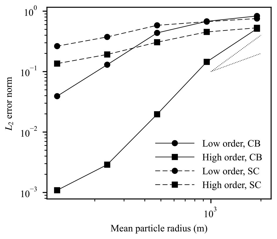
Figure 7 L₂ error norm versus mean particle radius for the cosine bell (CB) and slotted cylinder (SC) two-dimensional test cases with both low- and higher-order remapping. First- and second-order convergence gradients are also shown as the dotted lines.

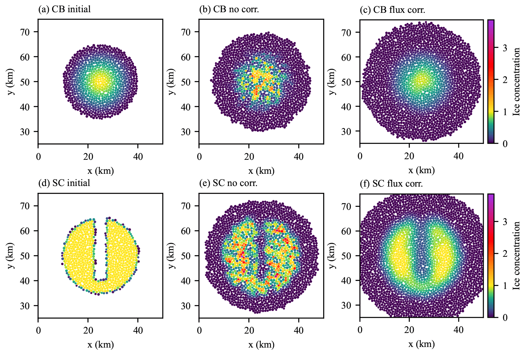
Figure 8 Stationary two-dimensional remapping test case with randomization of element orientations for cosine bell (CB: a–c) and slotted cylinder (SC: d–f) initial distributions. Shown are the initial sea ice concentration distributions (a and d), results without flux correction (b and e), and results with flux correction (c and f).

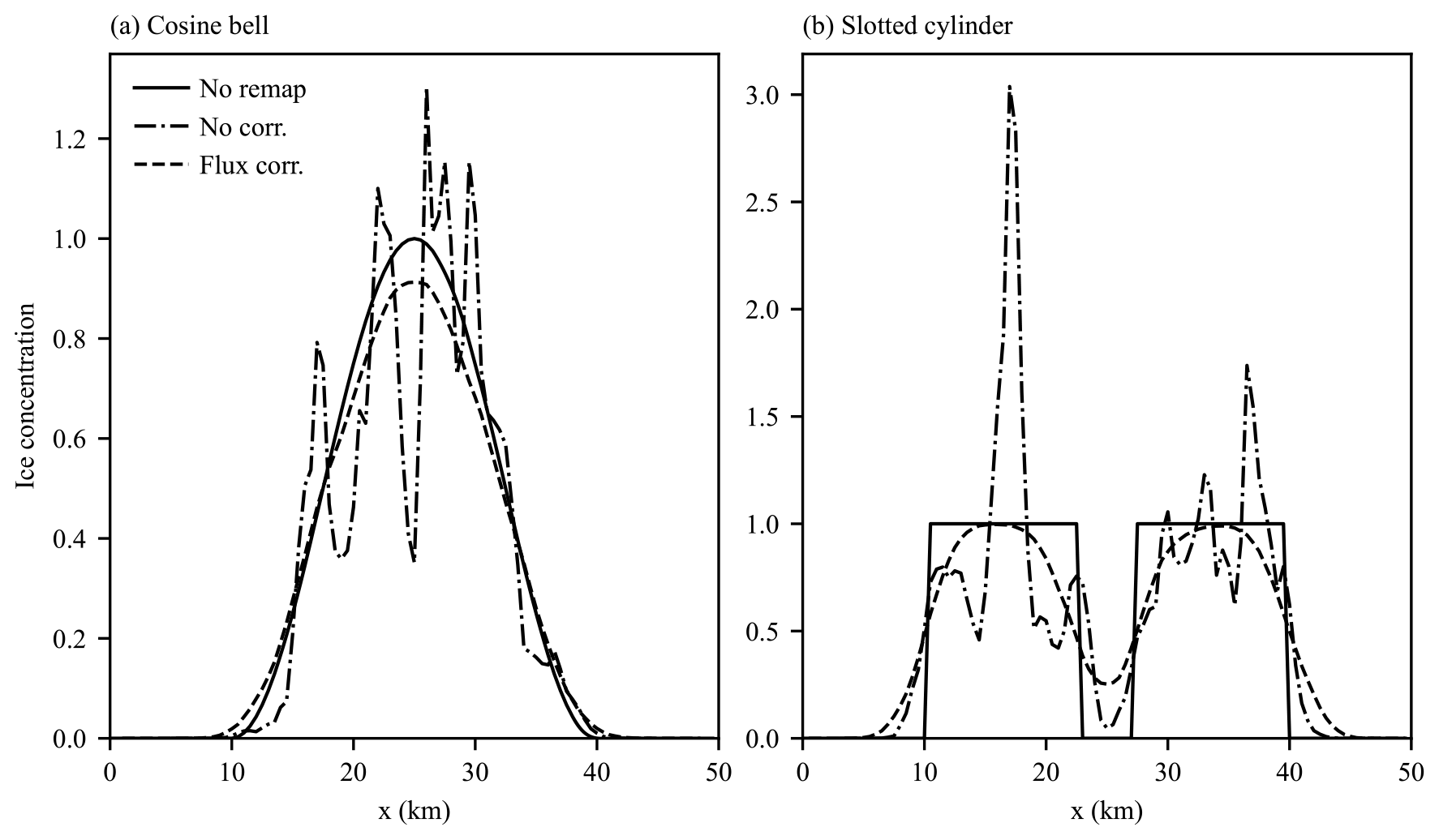
Figure 9 Cross section (y = 50 km) of ice concentration for the stationary two-dimensional test case with randomized orientations for the initial (a) cosine bell and (b) slotted cylinder particle distributions.

Next we study the error scaling properties of the remapping method. To do this we create various initial element distributions with different mean particle radii but the same relative distribution of radii. We rerun the simulations for these element distributions and record the L₂ error norm for each simulation. We calculate the L₂ error norm as

$$\begin{array}{}\text{(54)}& L_{\mathrm{2}}={\displaystyle \frac{{\sum }_i{e}_i\sqrt{c_i^{\mathrm{2}}-c_i^{\mathrm{02}}}}{{\sum }_i{e}_i\sqrt{c_i^{\mathrm{02}}}}},\end{array}$$

where the sum is over the final element distribution, e_i and c_i are the effective area and concentration of the final distribution, and $c_i^{\mathrm{0}}$ is the ice concentration for no remapping. In Fig. 7, the values of the L₂ error norm are plotted against the mean radius of the element distribution for both the cosine bell and slotted cylinder initial distributions as well as the low- and higher-order remapping methods. As can be seen from the figure the higher-order method has significantly lower errors than the low-order method for both initial distributions. The gradient of the slope for the smooth cosine bell distribution is also much higher than the slotted cylinder with its sharp discontinuities. It is also apparent that for the smooth cosine bell distribution the remapping method is approximately second-order accurate for the higher-order method.

4.3 Flux correction tests

Having demonstrated in Sects. 4.1 and 4.2 that the higher-order remapping method for uniform motion is capable of remapping the particle distribution with low numerical diffusion while preserving compatibility, we next turn to examining the effect of nonuniform motion and testing the ability of the flux correction algorithm described in Sect. 3.4 to correct the issues created by this motion. The first test we examine is a variation of the two-dimensional test used in the previous section. Instead of making the elements undergo uniform motion, we fix their positions and randomize the orientations of their associated polygons before each remapping. This introduces the overlaps and gaps between source polygons that might be expected from a general motion of the elements. As before, a total of 200 remappings are performed before the concentration distributions are examined. Figure 8b and e show the effect of these randomized orientations on the remapped ice concentration for the higher-order remapping scheme. As can be seen, while the general shape of the initial distributions is preserved, the randomization results in ice concentrations significantly larger than 1 for some elements (where elements overlapped) and ice concentration less than that expected for others (from gaps in the polygon distribution), with these effects taking on a random nature. Clearly, without correction this effect would have a seriously detrimental effect for any sea ice simulation. Figure 8c and f show the same final ice concentration distribution but generated with the flux correction scheme described in Sect. 3.4 performed after remapping. Now, ice concentrations are bounded correctly by [0,1], and the final distribution is smooth with results similar to those obtained in Sect. 4.2. Exactly the same result is not expected as the distribution of particles for remapping is different and the remapping method tested in Sect. 4.2 does not require the flux correction scheme. However, the similarity in the results indicates that the flux correction scheme works effectively and does not introduce significantly more numerical diffusion. This is also evident in the cross section of ice concentration shown in Fig. 9. Repeating the L₂ error scaling analysis in the previous section (Fig. 10) shows larger L₂ error norms for the uncorrected simulations, while the flux-corrected simulations show significantly lower errors and also show second-order convergence with mean particle size for the smooth cosine bell test case.

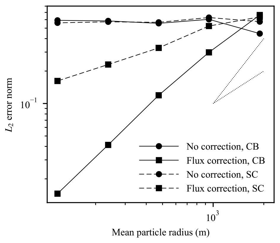
Figure 10 L₂ error norm versus mean particle radius for the cosine bell (CB) and slotted cylinder (SC) stationary two-dimensional test cases with randomized orientations with both low- and higher-order remapping. First- and second-order convergence gradients are also shown as the dotted lines.

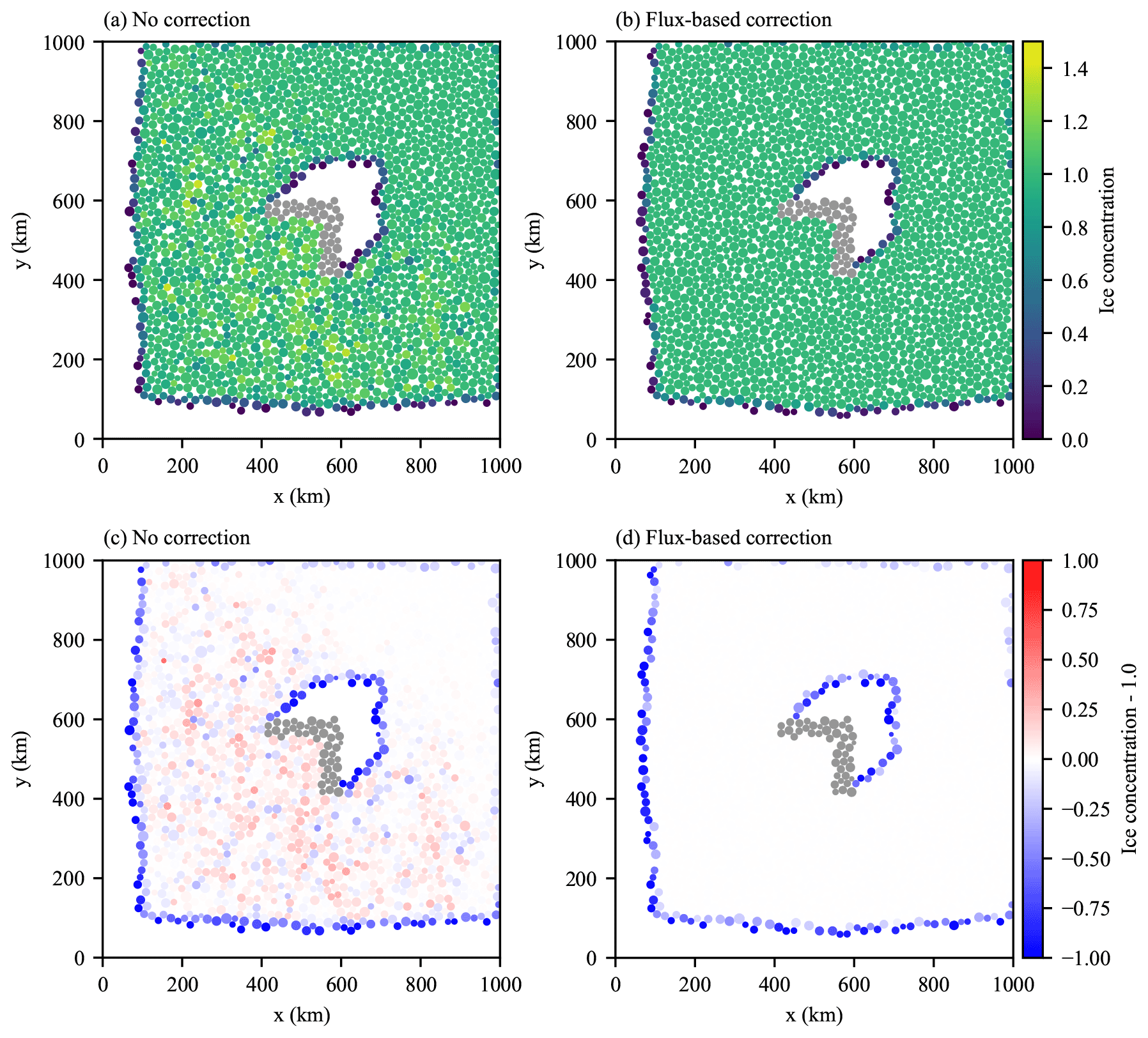
Figure 11 Island test case showing remapping without any correction (a, c) and with the flux-based correction (b, d). (a, b) Ice concentration and (c, d) the difference from an ice concentration of 1.0. Coastal elements comprising the central island are shown in grey.

To demonstrate the effect of the flux correction in more realistic situations we present two more test cases. In the first, adapted from Lipscomb et al. (2007), we have a square domain of size 1000 km by 1000 km with a random distribution of elements covering the domain generated by the algorithm of Liang et al. (2015). In the middle of the domain is an “L-shaped” island consisting of fixed coastal elements. Initial elements are coastal or sea ice elements according to the following. 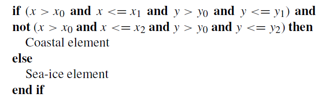Here, (x,y) is the position of the element center, x₀ and y₀ equal 400 km, x₁ and y₁ equal 600 km, and x₂ and y₂ equal 550 km. Elements have a mean element radius of ∼ 10 km, with non-coastal elements having a concentration of 1 everywhere. A constant wind forcing is applied to the elements with the x and y components of wind velocity both equal to 10 m s⁻¹, while the ocean is stationary. During the simulation the elements flow around the island, leaving an open-water wake behind it. Since the contact model used here consists of elastic repulsion without a representation of ridging, ice does not build up on the windward side of the island. The simulation is run for 2 d after which the element distribution is remapped to the destination element distribution with the higher-order scheme and either with or without the flux correction algorithm. Figure 11a and b show the effect on ice concentration of remapping without and with the flux correction, respectively. Figure 11c and d show the same but with a value of 1 subtracted from the ice concentration to highlight the excess ice concentration generated by the remapping when the flux correction is not used. These figures clearly show elements with concentration greater than 1 after remapping without flux correction and also show how the flux correction removes this excess concentration and results in a concentration field closer to the concentration field before remapping with a concentration of 1 most places within the pack. Elements on the edge of the ice pack and the edge of the island wake have concentrations less than 1, since during the remapping these elements were not fully covered by source elements.

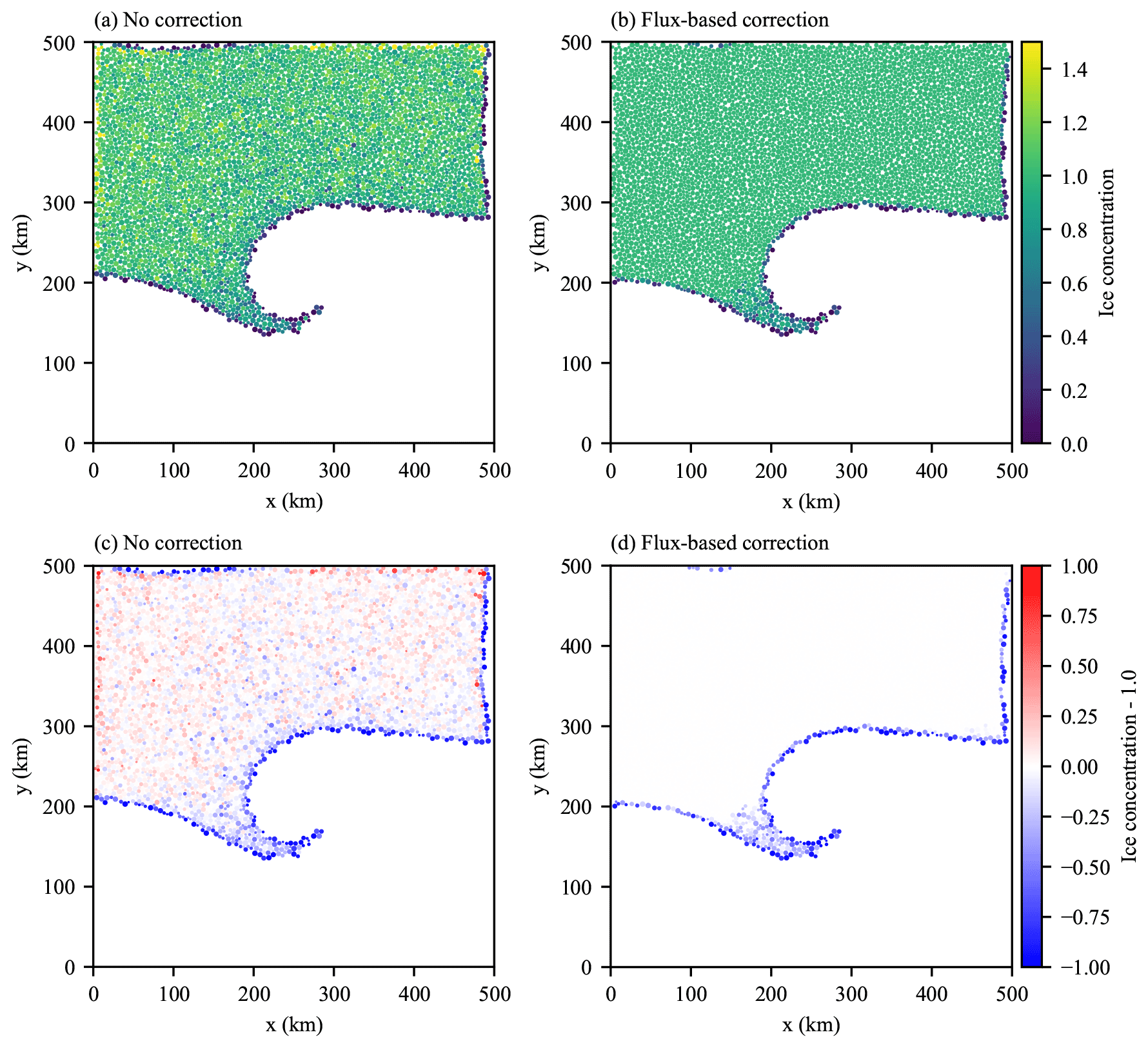
Figure 12 Vortex test case showing remapping without any correction (a, c) and with the flux-based correction (b, d). (a, b) Ice concentration and (c, d) the difference from an ice concentration of 1.0.

The final test case we examine is that from Flato (1993). Here the domain consists of a 500 km by 500 km closed square with the upper half (y > 250 km) initially filled with elements with a concentration of 1 and a mean radius of ∼ 2.5 km. The elements have the same air and ocean stress formulation and the same elastic repulsion contact model as the previous island test case. The ocean is again stationary, but the wind field, U_a, takes the form of a vortex with

$$\begin{array}{}\text{(55)}& {\mathit{U}}_{\mathrm{a}}\left(\mathit{r}\right)=min\left\{\mathit{\omega }\left|\mathit{r}\right|,{\displaystyle \frac{\mathit{\lambda }}{\left|\mathit{r}\right|}}\right\}\left(\mathit{k}\times {\displaystyle \frac{\mathit{r}}{\left|\mathit{r}\right|}}\right),\end{array}$$

where r is the position vector relative to the center of the vortex at (250, 200 km), ω is 0.5 × 10⁻³ s⁻¹, λ is 8 × 10⁵ m² s⁻¹, and k is the unit vertical vector. The simulation is run for 2 d and then the element distribution is remapped. As for the island test case, Fig. 12 shows that the flux correction scheme is capable of removing excess concentration caused by more realistic nonuniform motion of the elements for this test case.

5 Conclusions

Modeling sea ice dynamics with the discrete element method has the potential to enable the capture of the anisotropic deformation and fracture seen in observational data that are difficult to reproduce in continuum models. The DEM models, however, present a challenge due to convergence and overlap of the Lagrangian elements in simulations. To manage this element clustering, a deformed element distribution is periodically remapped to an undeformed distribution. This paper presents a geometrically based remapping algorithm designed to address the unique challenges of accurately remapping sea ice tracer fields for circular discrete elements. In particular, the method includes a representation of effective element area defined with a radical Voronoi tessellation for the undeformed element configuration that enables an accurate definition of area conservation in the case of 100 % sea ice concentration. Our remapping approach builds on conservative, bounds-preserving, and compatible algorithms developed for incremental remapping and applied to sea ice (Lipscomb and Hunke, 2001; Lipscomb and Ringler, 2005). In the case of uniform motion, the effective element area enables a complete coverage of the ice domain without overlap, and the method inherits the properties of the incremental remapping algorithms. In the case of nonuniform motion in which gaps and overlaps occur between the deformed effective element areas, monotonicity can be lost. To address this, we developed a novel flux-based correction method, which maintains conservation while correcting for bounds violations due to overlapping elements. Numerical examples are provided that demonstrate the second-order accuracy of the method, bounds preservation for both uniform and nonuniform motion, and compatibility between primitive and conserved tracer quantities.