Model development in practice: a comprehensive update to the boundary layer schemes in HARMONIE-AROME cycle 40

The parameterised description of subgrid-scale processes in the clear and cloudy boundary layer has a strong impact on the performance skill in any numerical weather prediction (NWP) or climate model and is still a prime source of uncertainty. Yet, improvement of this parameterised description is hard because operational models are highly optimised and contain numerous compensating errors. Therefore, improvement of a single parameterised aspect of the boundary layer often results in an overall deterioration of the model as a whole. In this paper, we will describe a comprehensive integral revision of three parameterisation schemes in the High Resolution Local Area Modelling – Aire Limitée Adaptation dynamique Développement InterNational (HIRLAM-ALADIN) Research on Mesoscale Operational NWP In Europe – Applications of Research to Operations at Mesoscale (HARMONIE-AROME) model that together parameterise the boundary layer processes: the cloud scheme, the turbulence scheme, and the shallow cumulus convection scheme. One of the major motivations for this revision is the poor representation of low clouds in the current model cycle. The newly revised parametric descriptions provide an improved prediction not only of low clouds but also of precipitation. Both improvements can be related to a stronger accumulation of moisture under the atmospheric inversion. The three improved parameterisation schemes are included in a recent update of the HARMONIE-AROME configuration, but its description and the insights in the underlying physical processes are of more general interest as the schemes are based on commonly applied frameworks. Moreover, this work offers an interesting look behind the scenes of how parameterisation development requires an integral approach and a delicate balance between physical realism and pragmatism.

1 Introduction

Due to ever-growing computer resources, numerical resolution of weather and climate models is steadily refined. Presently, limited area models operate routinely at resolutions of around 1 km and the first global intercomparison project for global storm-resolving models at resolutions of 5 km demonstrates that deep convective overturning processes are at least partly resolved by the new generation of weather and climate models (Stevens et al., 2019).

Prime atmospheric processes that remain to be parameterised at these scales are turbulent transport in the boundary layer, shallow cumulus convection, radiation, and cloud micro- and macrophysical processes of unresolved clouds. Traditionally, parameterisation of these processes has been developed as independent building blocks. The turbulence scheme describes the transport of heat, moisture, and momentum by the small-scale turbulent eddies in the boundary layer, whereas the convection scheme represents the transport by the larger-scale organised convective plumes. The cloud scheme aims to estimate the cloud fraction and the amount of condensed water.

Nowadays, it is recognised that the latter three parameterisation schemes need to be tightly coupled, as illustrated in Fig. 1. The cloud scheme requires information on the subgrid-scale variability of moisture and temperature as produced by the turbulence and convection scheme. Vice versa, the mixing by turbulence in the cloud boundary layer depends strongly on the cloud fraction. Clearly, optimisation of only one scheme will likely deteriorate the performance of another coupled scheme. This is why we describe in this paper the revision and optimisation of a tightly coupled triplet of parameterisation schemes for boundary layer turbulence, shallow cumulus convection, and clouds.

As stated by Jakob (2010), “Whereas early parameterisations development was aimed at finding suitable simple statistical relationships, modern parameterisations constitute complex conceptual models of the physical processes they are aiming to represent”. Indeed, more physically based parameterisations should be preferred as long as they improve the representation of essential processes, i.e. processes that significantly influence the resolved-scale variables. On the other hand, extra complexity in parameterisations should only be added if this does not imply introducing extra tunable parameters that cannot be constrained. Finding an acceptable level of physical realism and complexity without introducing too many tunable parameters that could give rise to overfitting, or even lead to an unstable system, is an important theme in this study.

The here-investigated parameterisations are part of the convection-permitting High Resolution Local Area Modelling – Aire Limitée Adaptation dynamique Développement InterNational (HIRLAM-ALADIN) Research on Mesoscale Operational NWP In Europe – Applications of Research to Operations at Mesoscale (HARMONIE-AROME) numerical weather prediction (Bengtsson et al., 2017) and climate model (Belus̆ić et al., 2020). Bengtsson et al. (2017), from hereon B17, present the HARMONIE-AROME configuration of cycle 40 (cy40) including a brief description of the reference model physics, noted as cy40REF. In contrast to B17, this paper provides a comprehensive description of the cloud, turbulence, and convection scheme. Moreover, we present numerous adjustments and improvements to the reference setup, included in a version referred to as cy40NEW. All these adjustments are accepted as the default options in the next release of HARMONIE-AROME, cycle 43.

The primary goal of these adjustments is to improve on what is considered one of the most important model deficiencies of HARMONIE-AROME cy40: a substantial underestimation of low cloud amount and overestimation of cloud base height.

The presented changes in the parameterisation schemes are primarily based on process studies and theoretical considerations. For example, long-term single-column model (SCM) runs are used to evaluate the turbulence scheme in terms of theoretical flux–gradient relationships, following the procedure of Baas et al. (2017). Based on these results, important modifications are made to the turbulence scheme. Additionally, several model intercomparison studies covering shallow cumulus, stratocumulus, and dry stable boundary layer conditions are used, most of which were based on observations collected during field campaigns. For these intercomparison cases, results of the Dutch Large Eddy Simulation (DALES, Heus et al., 2010) are compared in detail with SCM runs of HARMONIE-AROME. Finally, for the optimisation of the remaining uncertain parameters, we follow a more pragmatic approach by utilising 3-D model runs.

This paper can be considered a description of a substantial model update concerning several parameterisation schemes. Although the parameterisations are embedded in the HARMONIE-AROME model, we believe that our findings are more generally applicable in numerical weather prediction (NWP) and climate models. Even though the schemes in other models may differ in details, the parameterisations in HARMONIE-AROME are based on widely applied frameworks: a statistical cloud scheme, a (bulk) mass flux convection scheme, and a turbulence kinetic energy (TKE)-based turbulence scheme. Hence, the here-described modifications and the impact of certain parameters, or combinations of them, are useful for any atmospheric model that requires a parameterised representation of the clear and cloudy boundary layer.

We start with a description of the convection, turbulence, and cloud scheme in Sect. 2. Section 2.2 provides the first complete and detailed description of the shallow convection scheme. Documentation of the turbulence scheme can be found in Lenderink and Holtslag (2004) and Bengtsson et al. (2017). Therefore, only the parameters involved in the adjustments to the turbulence scheme are introduced in Sect. 2.3. Because of the comprehensive update to the statistical cloud scheme, a full description is provided in Sect. 2.4. Some of the adjustments introduced in Sect. 2 might seem arbitrary at first sight. However, Sect. 3 describes the experiments to motivate these adjustments. Several modifications are based on a comparison of SCM runs with large eddy simulation (LES) for the idealised case ARM (Sect. 3.1). SCM runs are also used to optimise the turbulence scheme against theoretical flux gradient relationships in Sect. 3.2. Section 3 further demonstrates the substantial improvements with the new configuration. For this, idealised cases of stratocumulus (Sect. 3.3), shallow convection (Sect. 3.1.2), and moderately stable conditions (Sect. 3.2) are used, as well as full 3-D model runs in Sect. 3.4. Finally, in Sect. 4, the discussions and conclusions are presented.

2 Parameterisation schemes

2.1 General framework

Before giving a more detailed description of the involved parameterisations in the next sections, we start by introducing the general parameterisation framework of the clear and cloud-topped boundary layer. The grid-box-averaged prognostic equations for the liquid water potential temperature θ_ℓ and the total water specific humidity q_t can be written as

$$\begin{array}{}\text{(1a)}& {\displaystyle }{\stackrel{\mathrm{‾}}{D}}_{\mathrm{t}}{\stackrel{\mathrm{‾}}{\mathit{\theta }}}_{\mathrm{\ell }}=-{\displaystyle \frac{\mathrm{1}}{\mathit{\rho }}}{\displaystyle \frac{\partial \mathit{\rho }\stackrel{\mathrm{‾}}{w^{\prime }{\mathit{\theta }}_{\mathrm{\ell }}^{\prime }}}{\partial z}}+Q_{\mathrm{rad}}\text{(1b)}& {\displaystyle }{\stackrel{\mathrm{‾}}{D}}_{\mathrm{t}}{\stackrel{\mathrm{‾}}{q}}_{\mathrm{t}}=-{\displaystyle \frac{\mathrm{1}}{\mathit{\rho }}}{\displaystyle \frac{\partial \mathit{\rho }\stackrel{\mathrm{‾}}{w^{\prime }{q}_{\mathrm{t}}^{\prime }}}{\partial z}}-G,\end{array}$$

where ρ is the average density, w the vertical velocity, G the autoconversion rate from condensed cloud water to rain water, and Q_rad the radiative heating tendency. The primes denote deviation from the grid mean values. The operator D_t represent a total time derivative, while the overbars denote the grid box mean for an arbitrary variable ϕ. Note that the condensation and evaporation tendencies are not present because we use a formulation in terms of moist conserved variables. The terms on the right-hand side of Eq. (1) are all subgrid scale and require a parameterised description.

The turbulent fluxes are parameterised using the eddy-diffusivity mass flux (EDMF) framework (Siebesma and Teixeira, 2000). This framework has been designed in order to facilitate a unified description of the turbulent transport in the dry convective boundary layer (Siebesma et al., 2007) and the cloud-topped boundary (Soares et al., 2004; Rio and Hourdin, 2008). More recent refinements and developments can be found in Neggers et al. (2009) and Sušelj et al. (2013). The EDMF approach is inspired by the notion that cumulus convection is usually rooted in the subcloud layer from which rising thermals transport moist buoyant air into the cumulus clouds aloft. It is therefore natural to decompose the turbulence into organised convective updrafts and a remaining part consisting of smaller-scale turbulent eddies:

$$\begin{array}{}\text{(2)}& \stackrel{\mathrm{‾}}{w^{\prime }{\mathit{\varphi }}^{\prime }}={\stackrel{\mathrm{‾}}{w^{\prime }{\mathit{\varphi }}^{\prime }}}^{\mathrm{turb}}+{\stackrel{\mathrm{‾}}{w^{\prime }{\mathit{\varphi }}^{\prime }}}^{\mathrm{conv}}.\end{array}$$

As long as the updraft fraction a_u is much smaller than unity, the convective transport can be conveniently parameterised in a mass flux (MF) framework as

$$\begin{array}{}\text{(3)}& {\stackrel{\mathrm{‾}}{w^{\prime }{\mathit{\varphi }}^{\prime }}}^{\mathrm{conv}}\approx {\displaystyle \frac{{\mathcal{M}}_{\mathrm{u}}}{\mathit{\rho }}}\left({\mathit{\varphi }}_u-\stackrel{\mathrm{‾}}{\mathit{\varphi }}\right),{\mathcal{M}}_{\mathrm{u}}=\mathit{\rho }{a}_{\mathrm{u}}{w}_{\mathrm{u}},\end{array}$$

where a bulk convective mass flux ℳ_u has been introduced and where w_u denotes the vertical velocity in the updraft. Mass flux mixing (Eq. 3) involves the conserved variables for temperature and humidity as well as momentum. Although convective momentum mixing is less efficient than scalar mixing (Li and Bou-Zeid, 2011), they are parameterised here similarly. Convective momentum transport is an active and important area of research (see, e.g. Schlemmer et al., 2017; Helfer et al., 2021; Saggiorato et al., 2020) but is not investigated this paper.

The remaining small-scale local turbulence is approximated by vertical diffusion by means of an eddy diffusivity (ED) approach:

$$\begin{array}{}\text{(4)}& {\stackrel{\mathrm{‾}}{w^{\prime }{\mathit{\varphi }}^{\prime }}}^{\mathrm{turb}}\approx -K{\displaystyle \frac{\partial \stackrel{\mathrm{‾}}{\mathit{\varphi }}}{\partial z}},\end{array}$$

which completes the EDMF framework in its simplest form. Note that the parameterisation task is now reduced to finding appropriate expressions for the mass flux ℳ_u the updraft fields ϕ_u and the eddy diffusivity K. One prime advantage of the EDMF approach is that the mass flux description of the updrafts can be active for both the clear and cloud-topped boundary layer so that the transition between these regimes can occur in a more continuous manner without the need for explicit switches or trigger functions.

There is a strong interplay between turbulence and convection (see Fig. 1). For example, the transport of heat by the convective thermals produced by the mass flux scheme will establish a neutral to slightly stable stratification in the upper part of the convective boundary layer, thereby suppressing the diffusive transport by the TKE scheme in this area (Lenderink et al., 2004). Besides, there is also a direct (coded) link between these schemes as the mass flux is used as a source term in a TKE budget equation that is used to parameterise the eddy diffusivity K (see Fig. 1). This interaction mimics the turbulence energy cascade in which turbulent kinetic energy cascades from the larger eddies down to the smaller eddies and will be further discussed in Sects. 2.3 and 3.1.1.

The last parameterisation involved in the modifications is the cloud scheme. The task of the cloud scheme is to estimate the subgrid-scale cloud fraction and the condensed water. A common approach to calculate cloud cover and condensed water is to assume a subgrid-scale distribution of humidity and temperature and to determine the cloud cover as the fraction of the distribution above saturation. A key element in such a statistical cloud scheme is the estimate of the subgrid-scale variance of the relative humidity. Important contributions to this variance are the convective (Eq. 3) and turbulent (Eq. 4) transport, establishing a strong link between the cloud scheme and the turbulence and convection parameterisations (Fig. 1).

The specific parameterisation implementations in HARMONIE-AROME are described in more detail in the upcoming subsections. The parameterisations of the convective mass flux ℳ_u and the updraft fields ϕ_u are discussed in Sect. 2.2. The eddy diffusivity parameterisation is discussed in Sect. 2.3 and finally the cloud scheme in Sect. 2.4.

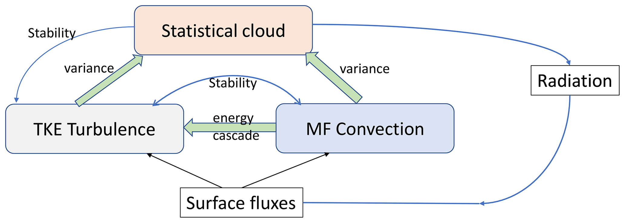
Figure 1 Schematic diagram illustrating the direct (thick arrows) and indirect (thin arrows) dependencies of parameterisation schemes with a focus on the schemes involved in the modifications.

2.2 Shallow convection scheme

The mass flux description is based on a dual mass flux approach (see, e.g. Neggers et al., 2009; from hereon N09) in which instead of one bulk updraft as in Eq. (3), we distinguish two updrafts: (1) a dry updraft describing all the thermals that do not convert into saturated updrafts in the cloud layer and (2) a moist updraft representing all updrafts that do reach the lifting condensation level (lcl) and continue their ascent in the cloud layer.

$$\begin{array}{}\text{(5)}& \mathit{\rho }{\stackrel{\mathrm{‾}}{w^{\prime }{\mathit{\varphi }}^{\prime }}}^{\mathrm{conv}}\approx {\mathcal{M}}_{\mathrm{dry}}\left({\mathit{\varphi }}_{\mathrm{u},\mathrm{dry}}-\stackrel{\mathrm{‾}}{\mathit{\varphi }}\right)+{\mathcal{M}}_{\mathrm{moist}}({\mathit{\varphi }}_{\mathrm{u},\mathrm{moist}}-\stackrel{\mathrm{‾}}{\mathit{\varphi }})\end{array}$$

As illustrated schematically in Fig. 2, we distinguish between two different convective boundary layer regimes: dry convective boundary layers with only a dry updraft and cloud-topped boundary layers with a dry and a moist updraft. Note that in contrast to B17 and N09, a stratocumulus-topped boundary layer in cy40NEW still uses a dry updraft (further discussed in Sect. 3.3).

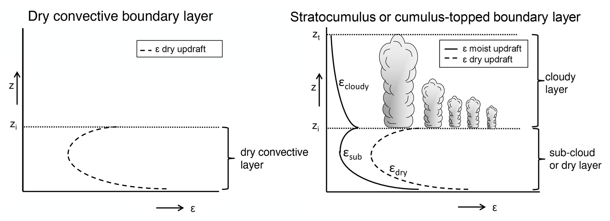
Figure 2 Schematic diagrams of the convective boundary layer regimes and the corresponding entrainment formulations (Eq. 8) of the dry (dashed line) and moist (solid line) updrafts. The inversion height and cloud top height are, respectively, denoted as z_i and z_t. Note that z_i can be different for the moist and dry updrafts and is therefore referred to as z_i,dry and z_lcl, respectively. The shape of the entrainment profiles reflects the inverse dependency on the vertical velocity of the updraft (Sect. 2.2.1). This is a modified version of Fig. 4 in B17.

The updraft profiles ϕ_u,i of updraft i ($i\in \mathit{\{}\mathrm{dry},\mathrm{moist}\mathit{\}}$) are determined by a conventional entraining plume model:

$$\begin{array}{}\text{(6)}& {\displaystyle \frac{\partial {\mathit{\varphi }}_{\mathrm{u},\mathrm{i}}}{\partial z}}=-{\mathit{\epsilon }}_{\mathrm{k}}({\mathit{\varphi }}_{\mathrm{u},\mathrm{i}}-\stackrel{\mathrm{‾}}{\mathit{\varphi }})+{\mathit{\mu }}_{\mathit{\varphi }},\end{array}$$

where ε_k denotes the fractional entrainment rate of the updraft and μ_ϕ represents cloud microphysical effects such as precipitation generation in the updraft (parameterised according to N09). The subscript k refers to different entrainment formulations for the dry updraft, the moist updraft in the subcloud layer, and the moist updraft in the cloud layer, i.e. $k\in \mathit{\{}\mathrm{dry},\mathrm{sub},\mathrm{cloudy}\mathit{\}}$. The various entrainment formulations are presented in Sect. (2.2.1).

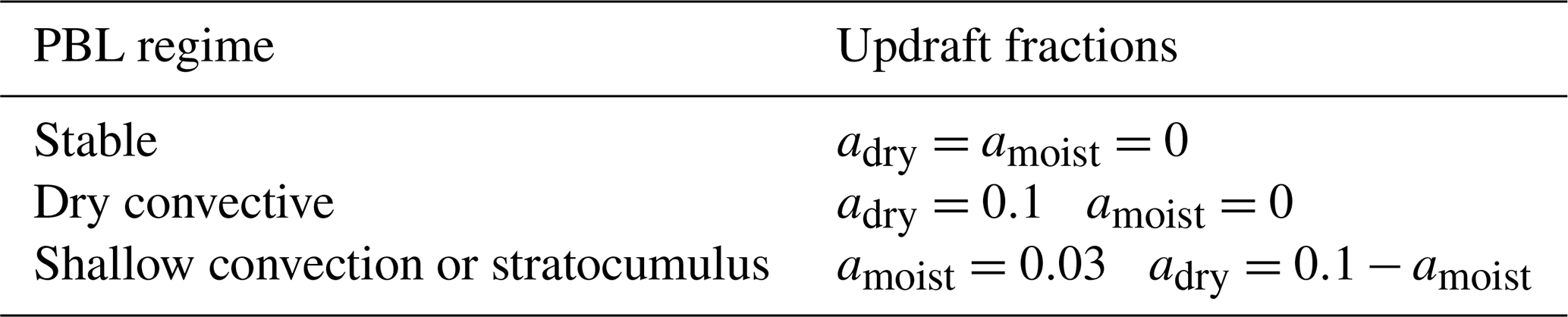
The updrafts are initialised at the lowest model level with a temperature and humidity that exceed the mean values at that level. The excess values are determined by assuming that the temperature and humidity are Gaussian distributed with a variance estimated from the turbulent surface fluxes following the standard surface layer scaling of Wyngaard et al. (1971). The initialisation temperature and humidity values are then given by their 1−a_u percentiles, where a_u denotes the fractional updraft area. Hence, larger variances and smaller area fractions give stronger excess values. The updraft vertical velocity at the lowest model level is simply initialised at 0.1 ms⁻¹ because the results are rather insensitive to the exact value. We refer to N09 for a more detailed description of the updraft initialisation. The updraft area fractions a_u are simply prescribed as fixed fractions as in (B17) instead of the more flexible updraft fractions in N09. These fixed updraft fractions depend on the diagnosed boundary layer regime (Table 1). Like in N09, the total updraft fraction under convective conditions is always 0.1. How the planetary boundary layer (PBL) regime is diagnosed is described in the next section.

Table 1 Updraft area fractions per PBL regime in cy40NEW. Constants a_dry and a_moist are used to determine the initialisation of temperature and humidity excess at the lowest model level of the corresponding updraft (like in N09). Together with the dry updraft vertical velocity, a_dry also determines the dry updraft mass flux (see Eq. 3). The moist updraft mass flux, however, is calculated independently of a_moist (see Sect. 2.2.2).

In addition to the updraft model for heat and moisture, a similar updraft equation is used for the vertical velocity w_u that can be used to estimate how deep the updrafts can penetrate (i.e. the height where w_u vanishes).

$$\begin{array}{}\text{(7)}& {\displaystyle \frac{\mathrm{1}}{\mathrm{2}}}{\displaystyle \frac{\partial w_{\mathrm{u},\mathrm{i}}^{\mathrm{2}}}{\partial z}}=a_{\mathrm{k}}{B}_{\mathrm{u},\mathrm{i}}-b_{\mathrm{k}}{\mathit{\epsilon }}_{\mathrm{k}}{w}_{\mathrm{u},\mathrm{i}}^{\mathrm{2}}\text{with}{B}_{\mathrm{u},\mathrm{i}}={\displaystyle \frac{g}{\stackrel{\mathrm{‾}}{{\mathit{\theta }}_{\mathrm{v}}}}}({\mathit{\theta }}_{\mathrm{v},\mathrm{u},\mathrm{i}}-{\stackrel{\mathrm{‾}}{\mathit{\theta }}}_{\mathrm{v}}),\end{array}$$

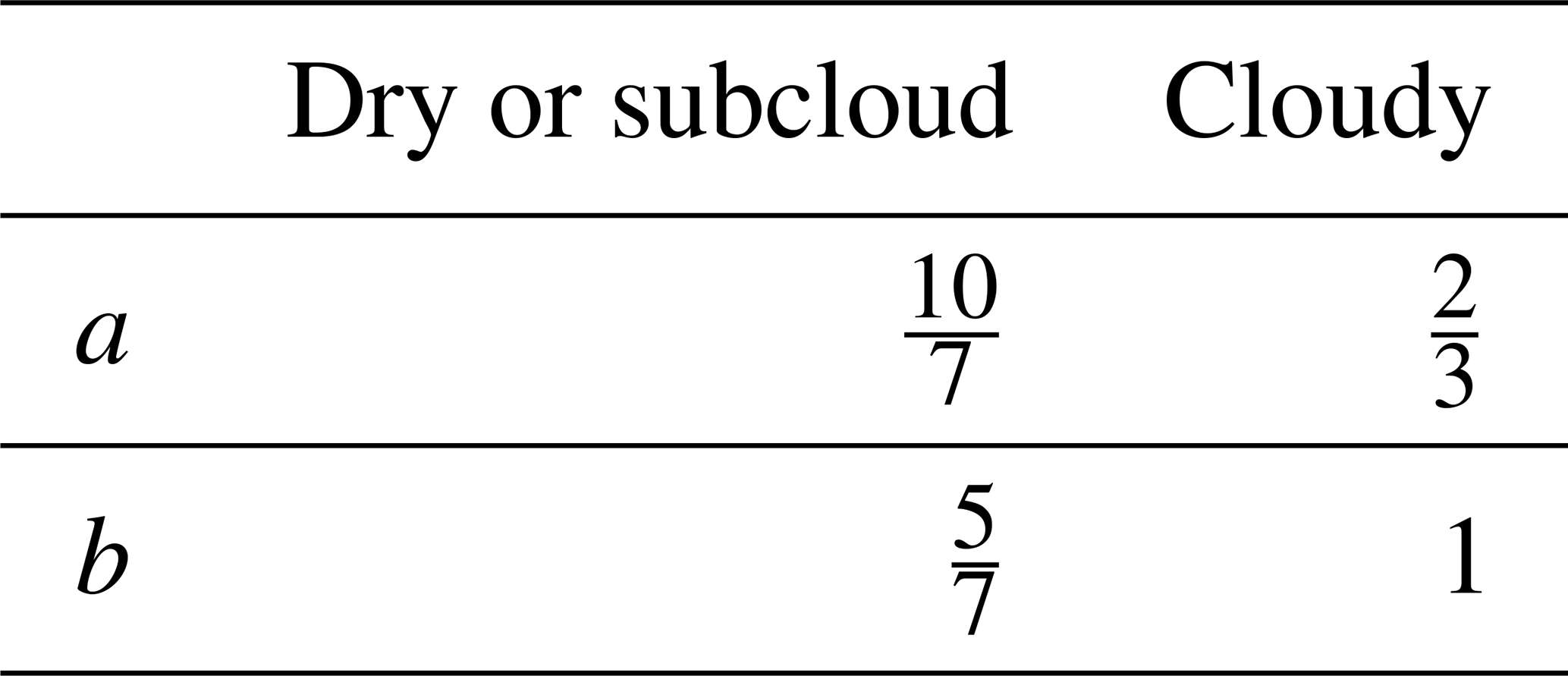
where w_u,i, B_u,i, and ${\mathit{\theta }}_{\mathrm{v},\mathrm{u},\mathrm{i}}$ are, respectively, updraft vertical velocity, buoyancy, and virtual potential temperature of updraft i. g is the acceleration of gravity. In Eq. (7), b_k and a_k are constants for dry ($k=\mathrm{dry},\mathrm{sub}$, i.e. dry convective boundary layer (CBL) or subcloud layer) and cloudy (k=cloudy) parts of the boundary layer. Note that Eq. (7) is a highly parameterised vertical velocity equation as effects of pressure are absorbed in the constants b_k and a_k (see, e.g. de Roode et al., 2012). In the literature, a large variety of values for a and b can be found. Based on LES, de Roode et al. (2012) showed that the accuracy of the vertical velocity equation in the cloud layer depends on a correct combination of a and b. They found good correspondence with LES results for the combination of constants in Bechtold et al. (2001), de Rooy and Siebesma (2010), and Rio et al. (2010), and we adopt these for the cloud layer (see Table 2). For dry updraft and subcloud layer part of the moist updraft, we adopt the formulation of Siebesma et al. (2007).

Table 2 Applied a and b coefficients in the vertical velocity equation (Eq. 7).

Fractional entrainment is not only applied in determining the updraft dilution in Eq. (6), but it also plays a role in the change of the mass flux with height, according to the following simple budget equation:

$$\begin{array}{}\text{(8)}& {\displaystyle \frac{\partial {\mathcal{M}}_{\mathrm{u}}}{\partial z}}=(\mathit{\epsilon }-\mathit{\delta }){\mathcal{M}}_{\mathrm{u}},\end{array}$$

where δ, the fractional detrainment, describes the outflow of updraft air into the environment. An accurate description of the lateral mixing between the updraft and the environment is key to every mass flux scheme (see, e.g. de Rooy et al., 2013). Hence, ε and δ are described in detail in the next sections.

2.2.1 Fractional entrainment

Previously, the entrainment coefficients of the HARMONIE-AROME convection scheme have been discussed only briefly (B17). Here, they are described in detail. Further motivation for the parameter settings and adjustments is provided in Sect. 3.

We need to specify the fractional entrainment factors, ε, for both updraft types. Moreover, for the moist updraft, a distinction is made between the dry subcloud layer and the moist cloudy layer (Fig. 2). As demonstrated by de Rooy and Siebesma (2008) and de Rooy and Siebesma (2010), the fractional entrainment in the cloudy layer is mainly a function of the vertical extent of the cloud layer and reflects the general notion that a deeper cloud layers hosts larger clouds with lower fractional entrainment rates.

The entrainment formulations for the non-cloudy layers are based on existing LES-based formulations with the inversion height, z_i, as a parameter (Siebesma et al., 2007). However, the inversion height is not known a priori. To provide a first estimate of the inversion height, we therefore release a test parcel with an entrainment formulation inversely proportional to the vertical updraft velocity (Neggers et al., 2002, and N09 Eq. 19). The test parcel is only used for diagnostic purposes and does not affect the ultimate convective transport. Also note that here inversion height is actually the height where the dry updraft vertical velocity becomes 0 (so including the overshoot into the inversion) or the lifting condensation level in the case of the moist updraft. A flow diagram showing the steps in the convection scheme leading to the ultimate inversion heights and corresponding entrainment formulations, as well as the diagnosed regime(s), is presented in Fig. 3.

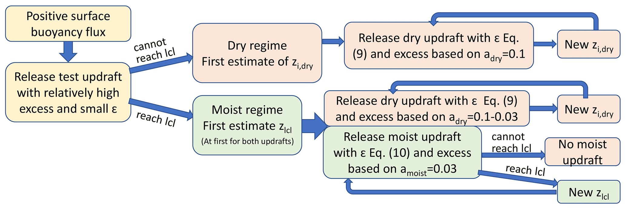
Figure 3 Schematic diagram of the subsequent steps in the shallow convection scheme to determine the ultimate inversion heights and corresponding entrainment formulations and the diagnosed regimes. After the test parcel (yellow), two iteration steps are done per entrainment formulation (red refers to dry and green to moist). Although the test parcel might have diagnosed a cloudy regime, it is possible that the ultimate moist updraft could not reach the lcl. In this case, no moist updraft is active (left panel of Fig. 2).

Apart from estimating z_i, the test parcel is also used to provide a first estimate of the boundary layer type to save computational time. If the updraft does not reach the lifting condensation level, the boundary layer type is dry convective with only a dry updraft (left panel of Fig. 2, and upper part of Fig. 1). If, on the other hand, the test parcel becomes saturated during its rise and condensation takes place, the boundary layer is estimated to be cloudy (right panel of Fig. 2, and lower part of Fig. 1). In this case, a dry and a moist updraft are considered. The relatively high excess and small ε of the test parcel ensure that cloudy regimes are not missed.

After diagnosing the PBL regime and the inversion height with the test updraft, the updraft rise is again calculated but this time with the area fractions from Table 1, leading to different initial excess values, and with the refined entrainment rates as defined below (see Fig. 3). Hereby, the inversion height will alter, but already after two iterations (fixed) with the refined entrainment formulations, the results show no significant change anymore. Note that the final PBL regime could be dry, whereas the test parcel passed the lcl due to iteration with lower initial excess and refined ε formulation (Fig. 3).

In the event of an ultimately cloudy PBL, the cloud layer depth is diagnosed, and if it exceeds a threshold (currently set to 4000 m), the model is supposed to resolve moist convection, and only dry convection remains parameterised. Note that this threshold value should decrease with increased spatial resolution.

Entrainment of the dry updraft

For any convective PBL regime, we need an entrainment formulation for the dry updraft. Based on LES results for a dry CBL, Siebesma et al. (2007) propose a formulation of ε as a fixed function of height, and we roughly adopt their formulation for the dry updraft:

$$\begin{array}{}\text{(9)}& {\mathit{\epsilon }}_{\mathrm{dry}}=c_{\mathrm{dry}}\left({\displaystyle \frac{\mathrm{1}}{z+a_{\mathrm{1}}}}+{\displaystyle \frac{\mathrm{1}}{z_{\mathrm{i},\mathrm{dry}}-z+a_{\mathrm{2}}}}\right)\text{for}z\le z_{\mathrm{i},\mathrm{dry}},\end{array}$$

where c_dry=0.4 (Siebesma et al., 2007) and z_i,dry is the dry updraft inversion height where the dry updraft stops rising. The shape of ε_dry using Eq. (9) (see Fig. 2a) reflects the expected increase in vertical velocity up to the middle of the dry convective boundary layer, resulting in decreasing ε values. From there, the updraft normally slows down, resulting in an increase of ε until the updraft finally stops at inversion height and ε becomes infinitely large. In practice, this ill definition of ε_dry is prevented by coefficient a₂ (similar to Soares et al., 2004). Again, similar to Soares et al. (2004), a₁ is introduced in cy40NEW to prevent very high entrainment values near the surface (see Sect. 3.1.2) and to reduce the dependence on the height of the lowest model level. Note that, due to the z⁻¹ dependence of the entrainment formulation (Eqs. 9 and 10), the initialisation of the temperature and humidity excess becomes rather independent of the height of the lowest model level. This is explained in detail in Appendix A of Siebesma et al. (2007).

Entrainment of the moist updraft in the subcloud layer

Also for the entrainment of the moist updraft in the subcloud layer (Eq. 10), we build on the formulation of Siebesma et al. (2007) (Eq. 9) and Soares et al. (2004), where the latter use a similar entrainment formulation as Eq. (10) but in a single updraft framework.

$$\begin{array}{}\text{(10)}& \begin{array}{rl}{\mathit{\epsilon }}_{\mathrm{sub}}& =c_{\mathrm{moist},\mathrm{sub}}\left({\displaystyle \frac{\mathrm{1}}{z+a_{\mathrm{1}}}}+{\displaystyle \frac{\mathrm{1}}{z_{\mathrm{lcl}}-z+\frac{z_{\mathrm{lcl}}}{\frac{{\mathit{\epsilon }}_{\mathrm{lcl}}}{c_{\mathrm{moist},\mathrm{sub}}}{z}_{\mathrm{lcl}}-\mathrm{1}}}}\right)\\ & \text{for}z<z_{\mathrm{lcl}}.\end{array}\end{array}$$

The formulation for the dry updraft (Eq. 9) needs to be adapted for the subcloud moist updraft for two reasons. Firstly, in contrast to the dry updraft, the moist updraft does not stop at inversion height (or cloud base), and therefore ε does not approach infinity. Instead, the entrainment at cloud base, noted as ${\mathit{\epsilon }}_{z_{\mathrm{lcl}}}$, is set to 0.002 m⁻¹, a reasonable value according to LES results (de Rooy et al., 2013; Siebesma et al., 2003). The apparently complicated last term in the dominator of Eq. (10) just ensures that the entrainment approaches its cloud base value apart from the term a₁. However, a₁ is negligible compared to typical z_lcl values. Secondly, the moist updraft represents stronger thermals than the dry updraft. LES results in Siebesma et al. (2007) reveal that the entrainment of stronger dry thermals (selected by changing the sampling criteria) corresponds to smaller c_dry values. Extending this to even stronger thermals that manage to become cumulus clouds, we set $c_{\mathrm{moist},\mathrm{sub}}=\mathrm{0.2}$.

As argued in Appendix B, ${\mathit{\epsilon }}_{z_{\mathrm{lcl}}}=\mathrm{0.002}$ m⁻¹ replaces ${\mathit{\epsilon }}_{z_{\mathrm{lcl}}}=\frac{\mathrm{1.65}}{z_{\mathrm{lcl}}}$ in cy40REF where the dependence on z_lcl was included to reflect that deeper boundary layers will contain larger updrafts with relatively small entrainment values.

Similar to Eq. (9), Eq. (10) reflects an inverse correlation between the expected updraft vertical velocity and the shape of the entrainment profile (see Fig. 2). Like in Eq. (9), a₁ is introduced in Eq. (10) of cy40NEW (see Appendix B and Sect. 3.1.2).

Entrainment of the moist updraft in the cloudy layer

The final entrainment profile to be defined is ε_cloudy. In contrast to Soares et al. (2004), the formulations of ε_sub and ε_cloudy are connected at cloud base. From cloud base, ε_cloudy will normally decrease with height related to increasing vertical velocity. Moreover, our bulk scheme should represent an ensemble of clouds and at higher levels only the largest, and fastest-rising, thermals, with relatively small entrainment values, will survive. Although the exact shape of LES-diagnosed entrainment profiles in the cloud layer will depend on the precise sampling method, a decrease proportional to z⁻¹ provides an acceptable fit and is used as a parameterisation.

$$\begin{array}{}\text{(11)}& {\mathit{\epsilon }}_{\mathrm{cloudy}}={\displaystyle \frac{\mathrm{1}}{z-z_{\mathrm{lcl}}+\frac{\mathrm{1}}{{\mathit{\epsilon }}_{z_{\mathrm{lcl}}}}}}\text{for}{z}_{\mathrm{lcl}}\le z,\end{array}$$

with, as mentioned before, ${\mathit{\epsilon }}_{z_{\mathrm{lcl}}}=\mathrm{0.002}$ m⁻¹ in cy40NEW. A comparison of Eq. (11) against LES-diagnosed entrainment rates is presented in Fig. 6 of de Rooy et al. (2013) and reveals a reasonably good correspondence, especially in comparison with estimates following a Kain–Fritsch type of formulation (Kain and Fritsch, 1990) as shown in Fig. 5 of de Rooy et al. (2013). Herewith, all entrainment rates in the dual mass flux scheme are defined.

2.2.2 The mass flux profile

The counterpart of entrainment is detrainment, δ, describing outflow of updraft air into the environment; see Eq. (8). Together with entrainment, the detrainment determines the change of mass flux with height. The mass flux profile is important as it, e.g. determines where the properties of the updraft are deposited in the environment. Besides, mass flux is used as input for the turbulence and cloud scheme (Sect. 2.3 and 2.4).

Equation (8) is not applied for the dry updraft where area fraction is assumed to be constant, so applying the vertical velocity Eq. (7) suffices to solve ℳ. Consequently, dry updraft mass flux simply varies with its updraft vertical velocity (like in N09).

For the moist updraft, we use the commonly applied mass flux closure at cloud base (Grant, 2001):

$$\begin{array}{}\text{(12)}& {\mathcal{M}}_{z_{\mathrm{lcl}}}=c_{\mathrm{b}}{w}_{*},\end{array}$$

where ${\mathcal{M}}_{z_{\mathrm{lcl}}}$ is the mass flux at cloud base and w_* is the usual convective velocity scaling derived from the surface buoyancy flux and using the cloud base as the boundary later depth (Grant, 2001). Further, c_b is a constant, set to 0.03 in cy40REF (according to Grant, 2001) and to 0.035 in cy40NEW (following Brown et al., 2002). In the subcloud layer, the moist updraft mass flux is imposed to increase linearly to the value at cloud base.

In the cloud layer, variations in the mass flux profile from case to case and hour to hour can be almost exclusively related to variations in the fractional detrainment as first pointed out by de Rooy and Siebesma (2008) (from hereon RS08). This is supported by numerous LES studies (e.g. Jonker et al., 2006; Derbyshire et al., 2011; Böing et al., 2012; de Rooy et al., 2013). Apart from empirical evidence, the much larger variation in δ and its strong link to the mass flux is explained by theoretical considerations in de Rooy and Siebesma (2010). Variations in δ partly arise from variations in cloud layer depth. This aspect is taken care of by evaluating and prescribing mass flux with a non-dimensionalised height, $\widehat{z}=\frac{(z-z_{\mathrm{lcl}})}{h}$ and mass flux, $\widehat{m}=\frac{{\mathcal{M}}_{\mathrm{u}}}{{\mathcal{M}}_{z_{\mathrm{lcl}}}}$, where h is the cloud layer depth, z_t−z_lcl, as diagnosed by the moist updraft. Here, z_t is the top of the cloud layer defined where w_u,moist becomes 0 ms⁻¹ and z_lcl corresponds to the cloud base height. Variations in the shape of the non-dimensionalised mass flux profile related to environmental conditions, like vertical stability and relative humidity, can be well described by a χ_crit dependence (RS08).

$$\begin{array}{}\text{(13)}& {\widehat{m}}_{*}=c_{\mathrm{1}}\langle {\mathit{\chi }}_{\mathrm{crit}}{\rangle }_{*}-c_{\mathrm{2}},\end{array}$$

where ${\widehat{m}}_{*}$ is the non-dimensionalised mass flux in the middle of the cloud layer (RS08) and χ_crit is the fraction of environmental air necessary to make updraft air just neutrally buoyant (Kain and Fritsch, 1990). The symbol 〈〉_* denotes the average from cloud base to the middle of the cloud layer. So 〈χ_crit〉_* represents environmental conditions the updraft experiences along its rise up to the middle of the cloud layer. Note that apart from environmental conditions, also the buoyancy of the updraft itself determines χ_crit (RS08). As discussed in RS08, Eq. (13) describes a physically plausible relationship: “Large values of 〈χ_crit〉_* can be associated with large clouds (of large radii) with high updraft velocities that have large buoyancy excesses and/or clouds rising in a friendly, humid environment”. For small 〈χ_crit〉_* values, the opposite can be expected. As discussed in RS08, updraft excess in LES (depending on sampling method) and in the model parameterisation will differ. Therefore, χ_crit values in LES and model will differ and consequently the optimal constants in Eq. (13). We apply c₁=5.24 (conform LES, RS08) and c₂=0.39. In addition, we limit ${\widehat{m}}_{*}$ between 0.05 (strongly decreasing mass flux) and 1 (no net decrease in mass flux). The upper boundary can be reached in stratocumulus layers where χ_crit values can be high due to a high humidity environment.

With ${\widehat{m}}_{*}$ known, and under the assumption that δ is constant with height (see, e.g. RS08) and that the entrainment varies as z⁻¹, the mass flux profile can be determined (for details, see RS08). The shape of the mass flux profile can vary from convex to concave up to the middle of the cloud layer; from there, mass flux decreases linearly to 0 at cloud layer top. Strong support for Eq. (13) can be found in Böing et al. (2012). Based on 90 LES runs covering a wide variety of relative humidity and stability of the environment, Böing et al. (2012) revealed a strong correlation of LES mass flux profiles with Eq. (13). Additionally, observations of trade wind cumuli mass flux reveal that the vast majority of the observations can be captured well with a simplified mass flux profile as described here (Lamer et al., 2015).

2.3 Turbulence scheme

In cycle 36 and older versions, HARMONIE-AROME made use of the CBR (Cuxart–Bougeault–Redelsperger) turbulence scheme (Cuxart et al., 2000; Seity et al., 2011). As discussed by de Rooy (2014) and B17, some model deficiencies can be related to the CBR scheme, most notably lack of cloud top entrainment. Therefore, the turbulence scheme HARATU (HArmonie with RAcmo TUrbulence) was implemented. HARATU is based on a scheme originally developed for the Regional Atmospheric Climate Model (RACMO) (van Meijgaard et al., 2012) and is described in detail in Lenderink and Holtslag (2004) (from hereon LH04). In comparison with LH04, some modifications were implemented in HARMONIE-AROME (see B17), mainly to ameliorate wind speed forecasts during stormy conditions. With HARATU, HARMONIE-AROME substantially improved on several aspects, especially wind speed (B17, de Rooy et al., 2010, 2017). On the other hand, together with updates of other parameterisations, HARATU contributed to the underestimation of low cloud cover and overestimation of cloud base height. Both output parameters are crucial for, e.g. aviation purposes, and eliminating these two specific shortcomings became a top priority in the HIRLAM consortium.

A full description of the turbulence scheme can be found in LH04 and B17 but for convenience here we introduce the components and parameters involved in the adjustments. In our turbulence scheme, the eddy diffusivity (see Eq. 4) is formulated as $K=l\sqrt{\mathrm{TKE}}$. The length-scale formulation in HARATU essentially consists of two length scales: one for (strongly) stable conditions, l_s, and one for weakly stable and unstable conditions, l_int. The latter, so-called integral length scale provides a “quadratic profile” for unstable conditions in the convective boundary layer and is also matched to surface similarity in near-neutral conditions. For more stable conditions, the common formulation,

$$\begin{array}{}\text{(14)}& l_{\mathrm{s}}=c_{\mathrm{m},\mathrm{h}}{\displaystyle \frac{\sqrt{\mathrm{TKE}}}{N}},\end{array}$$

is used, where c_m,h is a constant for momentum or heat, TKE is the turbulent kinetic energy, and N is the Brunt–Vaisala frequency.

To get the final length scale l_m,h for all stability regimes as applied in Eq. (4), we need to interpolate between the different length scales. The need for this arises because the different length scales do not match very well in the intermediate stability regimes; for example, the stable length scale approaches infinity for neutral stability. For this interpolation, the following ad hoc form is used:

$$\begin{array}{}\text{(15)}& {\displaystyle \frac{\mathrm{1}}{l_{\mathrm{m},\mathrm{h}}^{\mathrm{p}}}}={\displaystyle \frac{\mathrm{1}}{{\left\{\sqrt{(l_{\mathrm{int}}^{\mathrm{2}}+l_{\min }^{\mathrm{2}})}\right\}}^{\mathrm{p}}}}+{\displaystyle \frac{\mathrm{1}}{l_{\mathrm{s}}^{\mathrm{p}}}},\end{array}$$

where l_min is a minimum length scale:

$$\begin{array}{}\text{(16)}& {\displaystyle \frac{\mathrm{1}}{l_{\min }}}={\displaystyle \frac{\mathrm{1}}{l_{\mathrm{\infty }}}}+{\displaystyle \frac{\mathrm{1}}{\mathrm{0.5}{c}_{\mathrm{n}}\mathit{\kappa }z}},\end{array}$$

with c_n is a constant and κ is the von Karman constant. Note that, close to the surface, the length scale is limited to half the neutral length scale, c_nκz. Equations (15) and (16) are needed to interpolate smoothly between the stable length scale and the integral length scale near the surface and to provide a limit length scale for the free troposphere. We note that the square root term in Eq. (15) is in practice similar to taking the maximum of l_int and l_min, which is for instance needed to provide a background length scale for the free troposphere above the boundary layer where the integral length scale will be small or zero.

For most parameters in the length scale formulation, there is some theory that provides a reasonable range of values (LH04), but l_∞ is a tuning parameter and likewise the interpolation method is ad hoc based. In LH04, an inverse linear (p=1) but also an inverse quadratic (p=2) interpolation is discussed. In cy40REF, an inverse linear interpolation is used which suppresses mixing over a broad range of stability conditions. While the chosen form provides reasonably smooth transitions between the different stability regimes, results are sensitive to the interpolation and chosen constants, e.g. for l_∞, and this will be investigated in Sect. 3.2. Although the appropriate value for l_∞ is uncertain, this parameter significantly influences the entrainment flux and hence the preservation of the inversion at the top of the boundary layer (Sect. 3.4). The role of l_min resembles that of the free tropospheric length scale mentioned by Bechtold et al. (2008) and Köhler et al. (2011), who demonstrate the impact on inversion strength and consequently erosion of stratocumulus.

The last aspect of the turbulence scheme we discuss concerns the subcloud cloud interaction. The mass flux contribution to the total vertical transport results in a stable stratification in the upper part of the subcloud layer. Consequently, mixing by the TKE scheme will be strongly diminished in this area. These feedbacks between the mass flux and the turbulence scheme generally lead to an unrealistically strong inversion at cloud base. In many mass flux schemes, this runaway process is prevented by numerical diffusion which is dependent on the vertical resolution, and results of these schemes therefore tend to break down at very high resolution (Lenderink et al., 2004). For this reason, an ad hoc additional diffusion with constant 50⋅M_moist was added in cy40REF. In cy40NEW, we replaced this term with a more physically based energy cascade term.

Let us briefly discuss the underlying ideas of the energy cascade term. Its formulation is inspired by the prognostic equation of the mass flux vertical velocity variance (de Roode et al., 2000, Eq. 2.12 for w):

$$\begin{array}{}\text{(17)}& \begin{array}{rl}& {\displaystyle \frac{\partial a_{\mathrm{u}}(\mathrm{1}-a_{\mathrm{u}})(w_{\mathrm{u}}-w_{\mathrm{env}}{)}^{\mathrm{2}}}{\partial t}}=-\mathrm{2}{\mathcal{M}}_{\mathrm{u}}(w_{\mathrm{u}}-w_{\mathrm{env}}){\displaystyle \frac{\partial \stackrel{\mathrm{‾}}{w}}{\partial z}}\\ & -{\displaystyle \frac{\partial (\mathrm{1}-\mathrm{2}{a}_{\mathrm{u}}){\mathcal{M}}_{\mathrm{u}}(w_{\mathrm{u}}-w_{\mathrm{env}}{)}^{\mathrm{2}}}{\partial z}}-(\mathit{\epsilon }+\mathit{\delta }){\mathcal{M}}_{\mathrm{u}}(w_{\mathrm{u}}-w_{\mathrm{env}}{)}^{\mathrm{2}}\\ & +\mathrm{2}{a}_{\mathrm{u}}(\mathrm{1}-a_{\mathrm{u}})(w_{\mathrm{u}}-w_{\mathrm{env}})(S_{{\mathrm{w}}_{\mathrm{u}}}-S_{{\mathrm{w}}_{\mathrm{env}}}).\end{array}\end{array}$$

Here, S represents source terms and w_env is the vertical velocity of the updraft environment. Since for convective clouds $\Vert w_{\mathrm{env}}\Vert \ll w_{\mathrm{u}}$, w_env is, as usually, neglected. The left-hand side (LHS) of Eq. (17) represents the change of the organised (or updraft) vertical kinetic energy. The third term on the right-hand side (RHS), representing the impact of lateral mixing, is always a negative or sink term and can be related to the energy cascade from organised to smaller-scale eddies. We apply this term as a source in the TKE budget equation. However, considering the increased complexity of having two updraft types and to prevent too-high TKE values in the subcloud layer, we implemented the energy cascade term in an ad hoc simplified form:

$$\begin{array}{}\text{(18)}& \begin{array}{rl}{W}_{\mathrm{casc}}& =W_{\mathrm{casc},\mathrm{dry}}+W_{\mathrm{casc},\mathrm{moist}}=c{\mathit{\epsilon }}_{\mathrm{dry}}{w}_{\mathrm{u},\mathrm{dry}}^{\mathrm{2}}{\mathcal{M}}_{\mathrm{dry}}\\ & +F{w}_{\mathrm{u},\mathrm{moist}}^{\mathrm{2}}{\mathcal{M}}_{\mathrm{moist}},\end{array}\end{array}$$

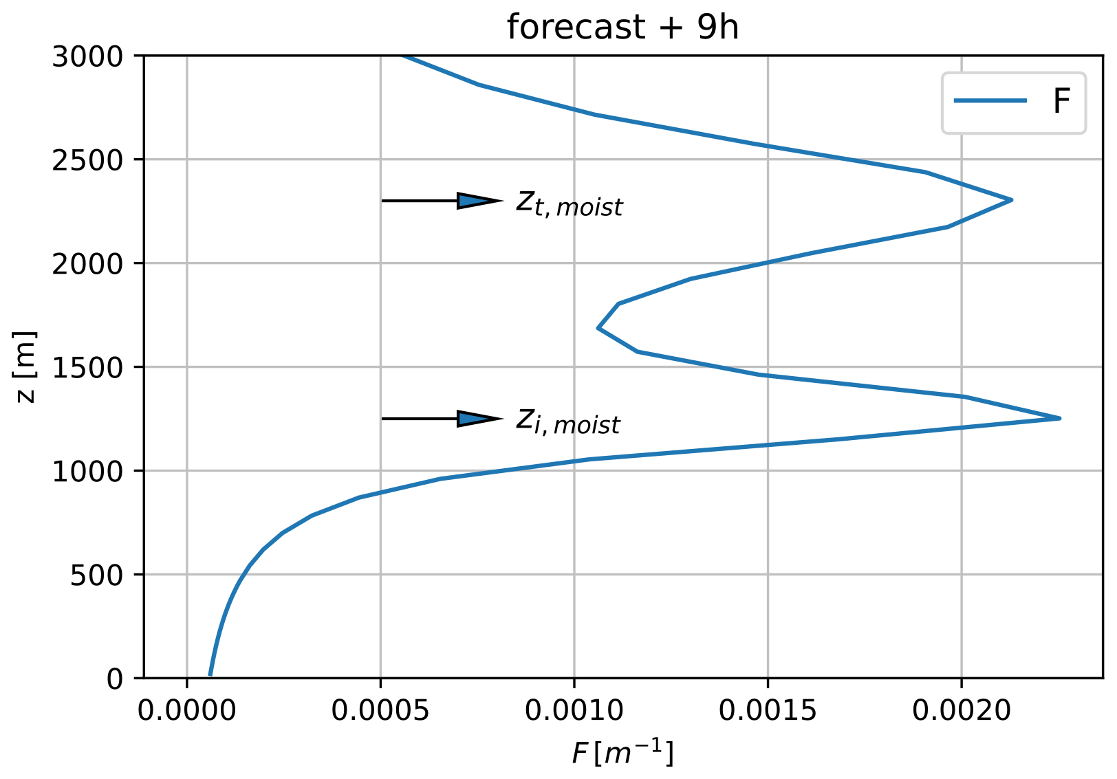
with function F:

$$\begin{array}{}\text{(19)}& F=E_{\mathrm{l}}\left({\displaystyle \frac{z}{z_{\mathrm{i}}}}\right)\left({\displaystyle \frac{\mathrm{1}}{\mathrm{1}+(\frac{z_{\mathrm{i}}-z}{Z_{\mathrm{wl}}}{)}^{\mathrm{2}}}}\right)+E_{\mathrm{t}}\left({\displaystyle \frac{\mathrm{1}}{\mathrm{1}+(\frac{z_{\mathrm{top}}-z}{Z_{\mathrm{wt}}}{)}^{\mathrm{2}}}}\right).\end{array}$$

Here, c=0.5, Z_wl=200 m, Z_wt=400 m. Further, E_l=0.002 m⁻¹ is a typical ε value near cloud base (consistent with Eqs. 10 and 11), and E_t=0.002 m⁻¹ corresponds to a similar peak at the level of neutral buoyancy but this time associated with detrainment in the upper part of the cloud layer. Figure 4 shows a typical profile of Eq. (19). By ignoring the detrainment term in the dry updraft contribution (Eq. 18) and applying function F (Eq. 19) for the moist updraft, too-large TKE values in the lower part of the boundary layer are prevented, whereas the contribution to TKE near cloud base and in the upper part of the cloud layer is supported.

Figure 4 Profile of F (Eq. 19) at the ninth simulation hour of the ARM case (Sect. 3.1) with cy40NEW.

Next to the usual dissipation, transport, buoyancies and shear terms, W_casc is added as a source term in the TKE budget equation. LES results in Sect. 3.1.1 substantiate the need for the energy cascade term and demonstrate the improved turbulent transport in cy40NEW due to the inclusion of the energy cascade term.

2.4 Statistical cloud scheme

Accurate predictions of clouds, liquid water, and ice are important because they have a large impact on radiation and therewith on several components of the model. This applies in particular to low boundary layer clouds such as stratocumulus and cumulus. In HARMONIE-AROME, high (ice) clouds are parameterised separately in a relative humidity scheme (B17) and are outside the scope of this paper. The here-presented derivations, ideas, and modifications concerning parameterisation of low clouds in HARMONIE-AROME are valuable for statistical cloud schemes in general.

The concept of parameterising clouds with a statistical cloud scheme was already pioneered by Sommeria and Deardorff (1977) and Mellor (1977) and makes use of the fact that cloud cover and liquid water content can be easily derived once subgrid variability of moisture and temperature is known. This concept has been further developed by Bougeault (1981) by assuming specific analytical forms of the joint probability density functions (PDFs) of total water specific humidity q_t and liquid water potential temperature θ_l, which are the relevant thermodynamic moist conserved variables. From several successive papers (Bechtold et al., 1995; Cuijpers and Bechtold, 1995; Bechtold and Siebesma, 1998), it became clear that it is sufficient to have reliable estimates of only the grid box variances of q_t and θ_l without making explicit assumptions on the shape of the underlying PDF. In statistical cloud schemes, relevant information on q_t and θ_l is captured in one variable called s, distance to the saturation curve, $s\equiv q_{\mathrm{t}}-q_{\mathrm{s}}$ with q_s being the saturation specific humidity. If we non-dimensionalise s by its standard deviation σ_s, $t\equiv s/{\mathit{\sigma }}_{\mathrm{s}}$, and presume a Gaussian PDF for t, the cloud fraction and liquid or ice water content can be written as a function depending only on the mean value of t:

$$\begin{array}{}\text{(20)}& \stackrel{\mathrm{‾}}{t}=({\stackrel{\mathrm{‾}}{q}}_{\mathrm{t}}-{\stackrel{\mathrm{‾}}{q}}_{\mathrm{s}})/{\mathit{\sigma }}_{\mathrm{s}}.\end{array}$$

Because ${\stackrel{\mathrm{‾}}{q}}_{\mathrm{t}}-{\stackrel{\mathrm{‾}}{q}}_{\mathrm{s}}$ is readily available in a model, the cloud parameterisation problem is simply reduced to estimating σ_s.

The base of statistical cloud schemes is an expression of variance in s in terms of variances and covariance of q_t and θ_l. Although the exact notation might be different, this expression should be the same for all schemes because the derivation is based on fundamental thermodynamics. Nevertheless, erroneous solutions can be found in the literature as well as in cy40REF. Therefore, we provide a step-by-step derivation of the variance in s in Appendix A1, which finally results in the following expression:

$$\begin{array}{}\text{(21)}& {\mathit{\sigma }}_{\mathrm{s}}^{\mathrm{2}}=\stackrel{\mathrm{‾}}{{s^{\prime }}^{\mathrm{2}}}={\mathit{\alpha }}^{\mathrm{2}}\stackrel{\mathrm{‾}}{{q_{\mathrm{t}}^{\prime }}^{\mathrm{2}}}-\mathrm{2}{\mathit{\alpha }}^{\mathrm{2}}\mathit{\beta }\stackrel{\mathrm{‾}}{q_{\mathrm{t}}^{\prime }{\mathit{\theta }}_{\mathrm{l}}^{\prime }}+{\mathit{\alpha }}^{\mathrm{2}}{\mathit{\beta }}^{\mathrm{2}}\stackrel{\mathrm{‾}}{{{\mathit{\theta }}_{\mathrm{l}}^{\prime }}^{\mathrm{2}}},\end{array}$$

with

$$\begin{array}{}\text{(22)}& {\displaystyle }\mathit{\alpha }={\displaystyle \frac{\mathrm{1}}{\mathrm{1}+\frac{L}{c_{\mathrm{p}}}{q}_{\mathrm{sl},\mathrm{T}}}},\mathit{\beta }=\mathit{\pi }{q}_{\mathrm{sl},\mathrm{T}}\text{(23)}& {\displaystyle }{\stackrel{\mathrm{‾}}{q}}_{\mathrm{sl},\mathrm{T}}={\displaystyle \frac{\partial q_{\mathrm{s}}\left({\stackrel{\mathrm{‾}}{T}}_{\mathrm{l}}\right)}{\partial T}},\end{array}$$

using the definition of the liquid water temperature:

$$\begin{array}{}\text{(24)}& T_{\mathrm{l}}\equiv T-{\displaystyle \frac{L}{c_{\mathrm{p}}}}{q}_{\mathrm{l}},\end{array}$$

and where L is the latent heat of vaporisation and c_p the heat capacity of dry air at constant pressure, and π is the Exner function, defined as $\mathit{\pi }=(\frac{p}{p_{\mathrm{0}}}{)}^{\frac{R_{\mathrm{d}}}{c_{\mathrm{p}}}}=\frac{T}{\mathit{\theta }}$, in which R_d is the gas constant of dry air and p₀ a reference surface pressure.

In the literature, several approaches exist to estimate σ_s (e.g. Golaz et al., 2002; Bechtold et al., 1995). Here, we provide a full description of our estimate in which we include the contribution to the variance by turbulence and convection as well as an additional term to cover other sources of variance.

If we neglect advection, precipitation, and radiation terms, the budget equations for (co)variances are (see, e.g. Stull, 1988)

$$\begin{array}{}\text{(25)}& {\displaystyle \frac{\partial \stackrel{\mathrm{‾}}{a^{\prime }{b}^{\prime }}}{t}}=-{\displaystyle \frac{\partial \stackrel{\mathrm{‾}}{w^{\prime }{a}^{\prime }{b}^{\prime }}}{\partial z}}-\left[\stackrel{\mathrm{‾}}{w^{\prime }{a}^{\prime }}{\displaystyle \frac{\partial \stackrel{\mathrm{‾}}{b}}{\partial z}}+\stackrel{\mathrm{‾}}{w^{\prime }{b}^{\prime }}{\displaystyle \frac{\partial \stackrel{\mathrm{‾}}{a}}{\partial z}}\right]-{\mathit{ϵ}}_{\mathrm{ab}},\end{array}$$

where $a,b\in \mathit{\{}{\mathit{\theta }}_{\mathrm{l}},q_{\mathrm{t}}\mathit{\}}$. The first term on the RHS of Eq. (25) is the transport term, the second and third terms represent the impact of the turbulent fluxes, and the last term covers dissipation. According to Bechtold et al. (1992), the transport term can be neglected during conditions with substantial cloud cover. The dissipation term, ϵ_ab, is modelled by a Newtonian relaxation back to isotropy:

$$\begin{array}{}\text{(26)}& {\mathit{ϵ}}_{\mathrm{ab}}={\mathit{ϵ}}_{\mathrm{ab},\mathrm{turb}}+{\mathit{ϵ}}_{\mathrm{ab},\mathrm{conv}}=c_{\mathrm{ab}}\left({\displaystyle \frac{{\stackrel{\mathrm{‾}}{a^{\prime }{b}^{\prime }}}^{\mathrm{turb}}}{{\mathit{\tau }}_{\mathrm{turb}}}}\right)+c_{\mathrm{ab}}\left({\displaystyle \frac{{\stackrel{\mathrm{‾}}{a^{\prime }{b}^{\prime }}}^{\mathrm{conv}}}{{\mathit{\tau }}_{\mathrm{conv}}}}\right),\end{array}$$

where c_ab is a constant and τ is a timescale for dissipation of turbulence (turb) or convection (conv). It is not clear if c_ab should be different for turbulence and convection. Moreover, a large variation in its value can be found in the literature (see, e.g. Bechtold et al., 1992; Redelsperger and Sommeria, 1981). For turbulence, τ can be approximated by

$$\begin{array}{}\text{(27)}& {\mathit{\tau }}_{\mathrm{turb}}={\displaystyle \frac{l_{\mathit{ϵ}}}{\sqrt{\mathrm{TKE}}}},\end{array}$$

where $l_{\mathit{ϵ}}=l_{\mathrm{m}}{c}_{\mathrm{0}}^{\mathrm{2}}$ is the dissipation length scale with c₀=3.75 (see LH04, and consistent with the turbulence scheme). In cy40REF, however, l_ϵ=l_m (discussed in Sect. A2). The timescale for convection can be related to the cloud depth divided by a typical cumulus updraft velocity (Lenderink and Siebesma, 2000). However, for simplicity, we adopt the approach of Soares et al. (2004) taking τ_conv=600 s.

Similar to dissipation, the turbulent fluxes in Eq. (25) consist of diffusive transport covered by the turbulence scheme:

$$\begin{array}{}\text{(28)}& \stackrel{\mathrm{‾}}{w^{\prime }{a}^{\prime }}=-K{\displaystyle \frac{\partial \stackrel{\mathrm{‾}}{a}}{\partial z}}=-l_{\mathrm{m},\mathrm{h}}\sqrt{\mathrm{TKE}}{\displaystyle \frac{\partial \stackrel{\mathrm{‾}}{a}}{\partial z}},\end{array}$$

where all stability factors are included in length scale l_m,h (LH04), and convective transport by the mass flux scheme:

$$\begin{array}{}\text{(29)}& \stackrel{\mathrm{‾}}{w^{\prime }{a}^{\prime }}={\mathcal{M}}_{\mathrm{u}}(a_u-\stackrel{\mathrm{‾}}{a}).\end{array}$$

As mentioned above, we neglect the transport term in Eq. (25) and assume a steady state, i.e. the LHS of Eq. (25), is 0. This means that production and dissipation of (co)variances are in balance. Note that the steady-state assumption is, at least for convection, debatable because the timescale for dissipation of convection is an order of magnitude larger than the typical time step of our model. On the other hand, cloud fractions for shallow, unresolved convection are usually small. Because we consider contributions of both turbulence and convection to the variance, we assume a balance between production and dissipation for both processes separately. Substituting Eqs. (26), (28), (29), τ_turb, and τ_conv in Eq. (25), including the assumptions mentioned above, leads to the following expressions:

$$\begin{array}{}\text{(30)}& {\displaystyle }{\stackrel{\mathrm{‾}}{a^{\prime }{b}^{\prime }}}^{\mathrm{turb}}=\mathrm{2}{\displaystyle \frac{l_{\mathrm{m},\mathrm{h}}{l}_{\mathit{ϵ}}}{c_{\mathrm{ab}}}}{\displaystyle \frac{\partial \stackrel{\mathrm{‾}}{a}}{\partial z}}{\displaystyle \frac{\partial \stackrel{\mathrm{‾}}{b}}{\partial z}}\text{(31)}& {\displaystyle }{\stackrel{\mathrm{‾}}{a^{\prime }{b}^{\prime }}}^{\mathrm{conv}}={\displaystyle \frac{-{\mathit{\tau }}_{\mathrm{conv}}}{c_{\mathrm{ab}}}}\left({\mathcal{M}}_{\mathrm{u}}(a_{\mathrm{u}}-\stackrel{\mathrm{‾}}{a}){\displaystyle \frac{\partial \stackrel{\mathrm{‾}}{b}}{\partial z}}+{\mathcal{M}}_{\mathrm{u}}(b_{\mathrm{u}}-\stackrel{\mathrm{‾}}{b}){\displaystyle \frac{\partial \stackrel{\mathrm{‾}}{a}}{\partial z}}\right).\end{array}$$

So, for example, total variance in θ_l due to turbulence and convection reads

$$\begin{array}{}\text{(32)}& \stackrel{\mathrm{‾}}{{{\mathit{\theta }}_{\mathrm{l}}^{\prime }}^{\mathrm{2}}}=\mathrm{2}{\displaystyle \frac{l_{\mathrm{h}}{l}_{\mathit{ϵ}}}{c_{\mathrm{ab}}}}{\left({\displaystyle \frac{\partial \stackrel{\mathrm{‾}}{{\mathit{\theta }}_{\mathrm{l}}}}{\partial z}}\right)}^{\mathrm{2}}-{\displaystyle \frac{\mathrm{2}{\mathit{\tau }}_{\mathrm{conv}}}{c_{\mathrm{ab}}}}\left({\mathcal{M}}_{\mathrm{u}}({\mathit{\theta }}_{\mathrm{l},\mathrm{up}}-\stackrel{\mathrm{‾}}{{\mathit{\theta }}_{\mathrm{l}}}){\displaystyle \frac{\partial \stackrel{\mathrm{‾}}{{\mathit{\theta }}_{\mathrm{l}}}}{\partial z}}\right).\end{array}$$

Note that both turbulence and convection have a positive contribution to variance.

In the absence of convection and no noticeable amount of turbulent activity, variance will still be non-zero. In nature, other sources of variance exist like surface heterogeneity, horizontal large-scale advection, mesoscale circulations, and gravity waves. Instead of imposing a minimum value to variance to cover these sources, we apply an extra variance term with the characteristics of a relative humidity scheme. This additional term was already introduced in de Rooy et al. (2010), demonstrating its beneficial impact, and has been included in the HARMONIE-AROME reference code since cycle 36. Here, a more elaborate description of the additional variance term is given.

Let us assume a statistical cloud scheme with a uniform distribution of a fixed width 2Δ. Tompkins (2005) shows that such a statistical cloud scheme can be considered a RH scheme with

$$\begin{array}{}\text{(33)}& \mathrm{\Delta }=(\mathrm{1}-{\mathrm{RH}}_{\mathrm{crit}})q_{\mathrm{s}},\end{array}$$

with RH_crit representing the relative humidity where cloud fraction starts to be non-zero. The corresponding cloud fraction reads

$$\begin{array}{}\text{(34)}& a_{\mathrm{c}}=\mathrm{1}-\sqrt{{\displaystyle \frac{\mathrm{1}-\mathrm{RH}}{\mathrm{1}-{\mathrm{RH}}_{\mathrm{crit}}}}}.\end{array}$$

The variance of such a uniform distribution is

$$\begin{array}{}\text{(35)}& {\mathit{\sigma }}_{q_{\mathrm{t}}}^{\mathrm{2}}={\displaystyle \frac{\mathrm{1}}{\mathrm{3}}}{\mathrm{\Delta }}^{\mathrm{2}}.\end{array}$$

Tompkins (2005) and Quaas (2012) demonstrated that a RH scheme as well a statistical cloud scheme with a fixed width distribution could be written purely in terms of specific humidity fluctuations; i.e. Eq. (21) reduces to

$$\begin{array}{}\text{(36)}& {\mathit{\sigma }}_{\mathrm{s}}^{\mathrm{2}}=\stackrel{\mathrm{‾}}{{s^{\prime }}^{\mathrm{2}}}={\mathit{\alpha }}^{\mathrm{2}}\stackrel{\mathrm{‾}}{{q_{\mathrm{t}}^{\prime }}^{\mathrm{2}}}={\mathit{\alpha }}^{\mathrm{2}}{\mathit{\sigma }}_{\mathrm{qt}}^{\mathrm{2}}.\end{array}$$

The combination of Eqs. (33), (35), and (36) leads to the following expression for RH_crit:

$$\begin{array}{}\text{(37)}& {\mathrm{RH}}_{\mathrm{crit}}=\mathrm{1}-{\displaystyle \frac{\sqrt{\mathrm{3}}}{\mathit{\alpha }}}\left({\displaystyle \frac{{\mathit{\sigma }}_{\mathrm{s}}}{q_{\mathrm{s}}}}\right).\end{array}$$

In HARMONIE-AROME, we introduced the additional standard deviation term:

$$\begin{array}{}\text{(38)}& {\mathit{\sigma }}_{\mathrm{s},\mathrm{extra}}=c\mathit{\alpha }{q}_{\mathrm{s}}.\end{array}$$

With c=0.02, this leads to a constant RH_crit=96 % (Eq. 37). Note that due to pre-factor α in Eq. (38), RH_crit becomes independent of α. For typical atmospheric conditions, α≃0.4 in the boundary layer, while higher up in the atmosphere α will asymptote towards unity. Therefore, without pre-factor α in Eq. (38), RH_crit would vary from ≃91 % in the boundary layer to ≃96 % in the upper atmosphere. However, sources of variance, not related to turbulence or convection, are particularly found higher up in the atmosphere (see, e.g. Quaas, 2012) and are, e.g. related to advection of long-lived cirrus clouds into the model grid box. Therefore, RH_crit should at least not increase with height. More investigation is needed to optimise the (height-dependent) formulation of the additional variance term. The total variance in s is the sum of the contributions from turbulence, convection, and Eq. (38).

From the description above and Appendix A, it becomes clear that a statistical cloud scheme contains many uncertain terms and constants. We do not claim that our choices are all optimal. However, in comparison with the original scheme, the new setup is at least built upon a correct derivation of the thermodynamical framework. This is, e.g. important for the formulation of thermodynamic coefficients (Eq. 22). Therefore, we believe the new setup is more suitable as a starting point for further improvements. Some suggestions to do so are discussed in Sect. 3.1.2.

3 Argumentation and evaluation of model updates

This paper describes a large variety of modifications to the current reference cloud, turbulence, and convection parameterisations. Argumentation of these adjustments is diverse. For example, part of the changes to the cloud and turbulence scheme have a theoretical basis, namely thermodynamics and surface layer similarity, respectively. Other modifications are substantiated by an in-depth comparison of 1-D model results with LES for several idealised intercomparison cases. Lastly, optimisation of some more uncertain model parameters is based upon evaluation of full 3-D model runs. Considering the large number of modifications and mutual influences, it is impossible to discuss the separate and incremental impact of them all. Instead, we focus on the performance of two HARMONIE-AROME configurations: firstly, the reference HARMONIE-AROME setup as described in B17, cy40REF, and, secondly, the new configuration, cy40NEW, as proposed in this paper. Nevertheless, all adjustments are substantiated and the isolated impact of several of them is demonstrated. An overview of all modifications is presented in Table D1 in Appendix D.

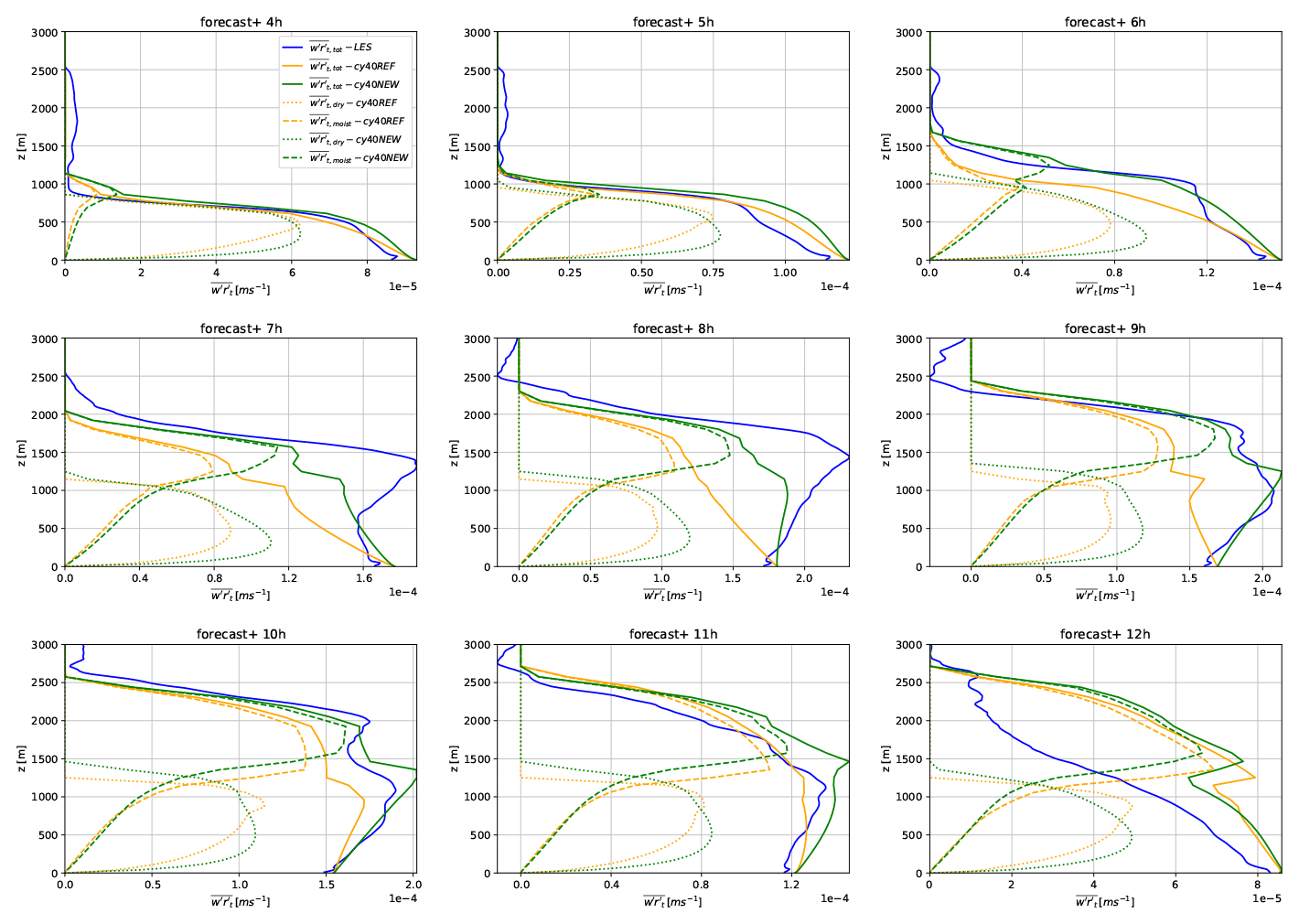
Figure 5 Total turbulent transport and transport by the dry and moist updraft (m s⁻¹) of the mixing ratio total humidity r_t during all convective hours of the ARM case, corresponding to simulation hours at +4 to +12 h. Plotted is total turbulent transport of cy40REF (orange solid line), cy40NEW (green solid line), and the total turbulent transport by the LES (blue). The dry updraft transport is shown as a dotted line (cy40REF in orange; cy40NEW in green). Similarly, the dashed lines show the transport by the moist updraft. Note that the x-axis scale is not constant.

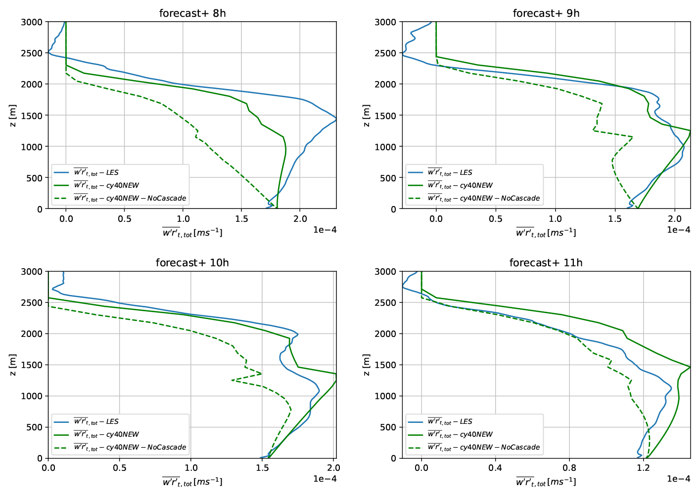
Figure 6 The kinematic total turbulent transport (m s⁻¹) during the last 4 h of the ARM convective period. Plotted is the transport according to LES (blue), cy40NEW (green), and cy40NEW but without energy cascade (green dashed). Note that the x-axis scale is not constant.

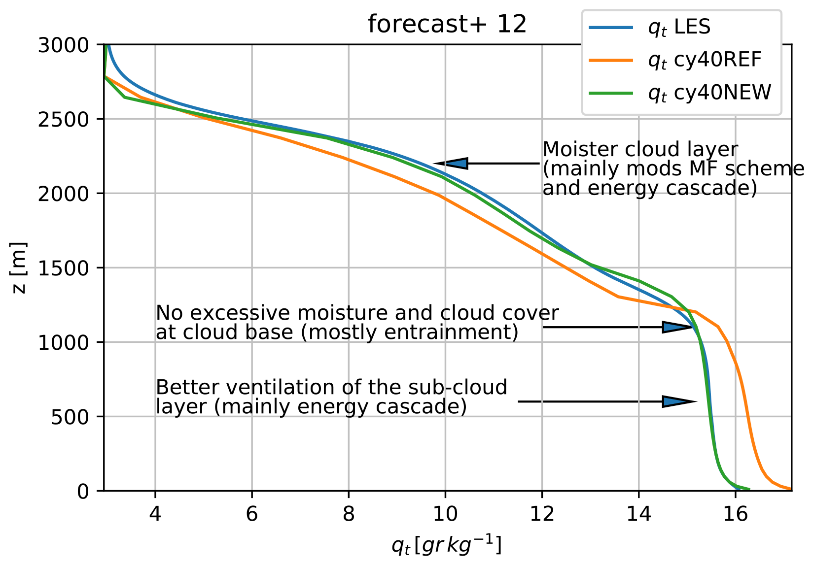
Figure 7 ARM case specific humidity profile after 12 h of simulation. These profiles can be seen as the accumulated impact of the total turbulent humidity transport during the ARM case.

Many of the proposed adaptations are the result of a comparison of 1-D model with LES results as obtained with the DALES model (Heus et al., 2010). For an accurate comparison between LES and HARMONIE-AROME at the current model resolution, LES results are diagnosed as the mean over HARMONIE-sized subdomains. In the ARM shallow cumulus case, for example, the turbulent transport in LES is the mean turbulent transport diagnosed in 100 subdomains of 2.5×2.5 km², the current operational resolution of HARMONIE-AROME. However, differences between the mean over HARMONIE-sized subdomains and the mean across the full LES domain are generally small. We start in Sect. 3.1 with an elaborated comparison of 1-D model with LES results for the ARM case. This investigation involves many components of the parameterisations and several modifications are based on the ARM case. By making use of Monin–Obukhov theory (following Baas et al., 2017), important changes to the turbulence scheme are substantiated in Sect. 3.2. This section also shows the performance under moderately stable conditions in the GABLS1 case (Beare et al., 2006). Section 3.3 mainly demonstrates the impact of the modifications on three stratocumulus cases. Finally, long-term and case-based verification with the 3-D model is presented in Sect. 3.4. This section demonstrates the large improvement with the updates in cy40NEW on low clouds but also elucidates the beneficial impact on precipitation.

3.1 ARM case

The ARM case (Brown et al., 2002), based on observations, describes a diurnal cycle of shallow convection above land: initiation of moist convection, gradual deepening of the cloudy layer, and finally collapse of the cumulus cloud layer. Such a dynamical case poses higher demands to convection parameterisation than, e.g. the steady-state Barbados Oceanographic and Meteorological Experiment (BOMEX) case over the sea (Holland and Rasmusson, 1973) and is therefore more suitable for optimisation purposes. To make optimal use of the dynamical character of the ARM case and to avoid a possible focus on the best results, we present results of all hours during the moist convective period (simulations from +4 to +12 h). The SCM runs for ARM use 79 vertical levels with the lowest model level at approximately 10 m.

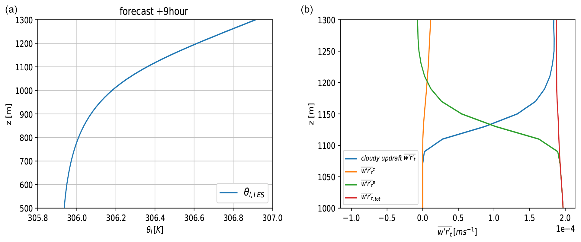
Figure 8 LES results around the cloud base inversion height for the ARM case at the ninth simulation hour. Panel (a) shows the θ_l profile, whereas (b) presents a decomposition of the kinematic turbulent moisture fluxes (m s⁻¹). Plotted are LES cloudy updraft flux (blue), small-scale subplume transport (orange), small-scale environmental transport (green), and total transport (red). Note the different y-axis scale.

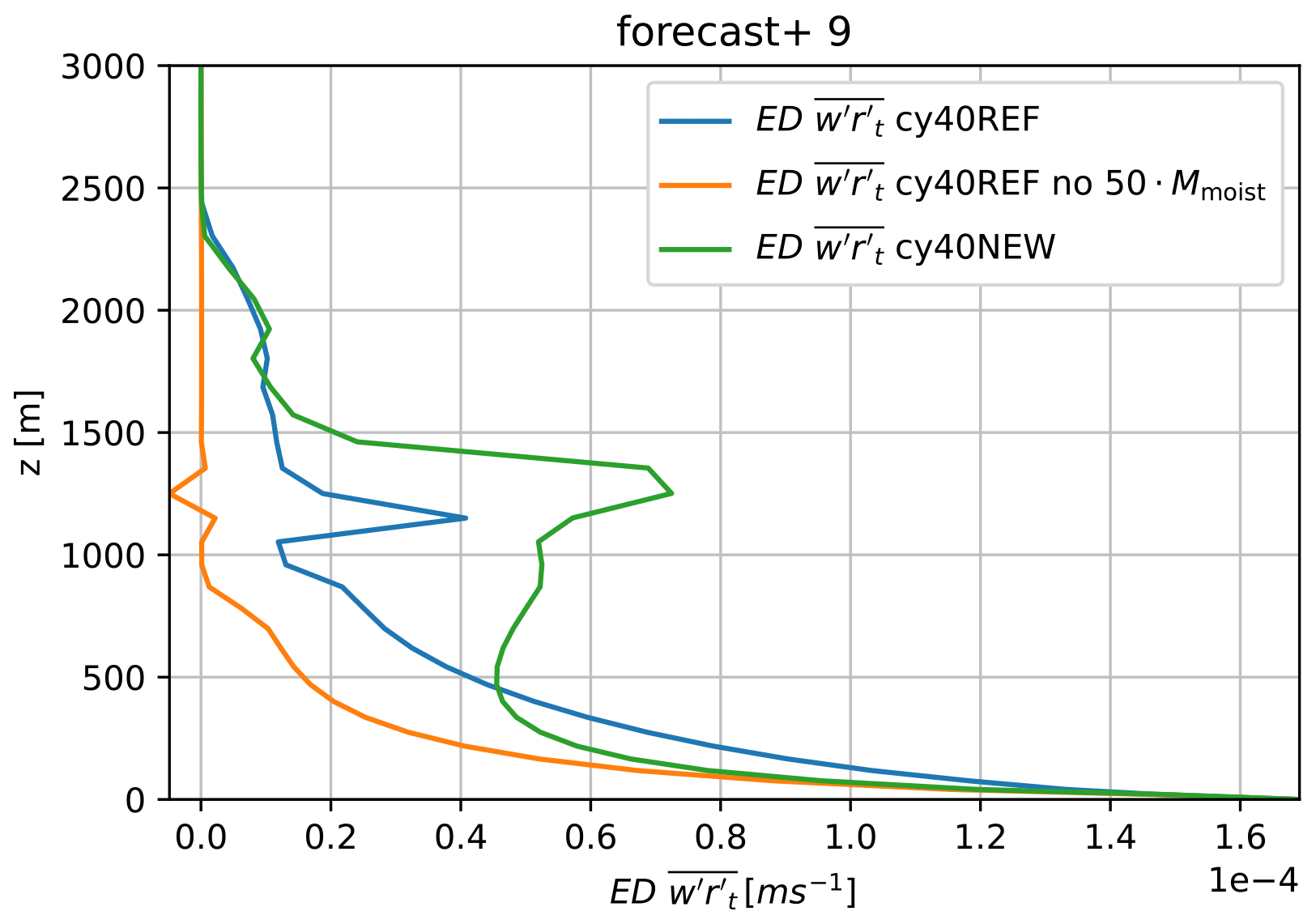
Figure 9 The eddy diffusivity (ED) turbulent moisture transport for ARM at the ninth simulation hour with three different model versions: cy40REF (blue), cy40REF but without 50⋅M_moist term (see Sect. 2.3) (orange), and cy40NEW (green).

3.1.1 ARM: mass flux and total turbulent transport

With the current operational resolution of HARMONIE-AROME, turbulent transport in the ARM case is fully unresolved and is presented as the sum of parameterised convective and diffusive turbulent transport. In LES, however, shallow convection and the bulk part of the diffusive transport is resolved. By sampling LES data in the cloud layer, we can estimate that part of the total turbulent transport that should be described by a convection scheme. Although the convective transport by LES should be interpreted as a rather crude estimate, it is also the best available way to study the performance of our mass flux convection scheme in the cloud layer. A detailed description of such an evaluation is provided in Appendix B and indicates that the convective transport in HARMONIE-AROME is underestimated in the first half of the convective period in the ARM case, but modifications to the convection scheme in cy40NEW result in a clear reduction of this underestimation (Appendix B).

However, the ultimate goal of a convection and turbulence scheme is to provide an accurate estimate of the total turbulent transport. After all, the vertical divergence of the total turbulent transport determines the tendencies of the prognostic model variables. Whereas LES convective transport should be interpreted as an estimate, depending on the sampling method, LES total turbulent transport during the ARM case will be close to observed values. Besides, in contrast to convective transport, LES provides the total turbulent transport for the complete atmosphere, including the subcloud layer. Figure 5 shows the total turbulent transport of humidity by the model versions and LES, including the LES subgrid-scale parameterised contribution. Plots of heat transport provide a similar behaviour (not presented). In general, both model versions underestimate total turbulent transport but the new configuration results in a considerable improvement. Drying of the subcloud layer, i.e. increasing total turbulent transport with height, in the second half of the convective period is almost absent in the original configuration and better captured with cy40NEW. This improvement is mainly related to inclusion of the energy cascade (Eqs. 18 and 19) as demonstrated in Fig. 6. Figure 6 further reveals that the energy cascade smoothens wiggles in turbulent transport around the inversion at cloud base. Figure 7 shows the humidity profiles at the end of the convective period, therewith reflecting the accumulated impact of turbulent transport during the ARM case. There is a close agreement between the humidity profiles of Cy40NEW and LES, whereas the cy40REF run clearly leads to a too-moist subcloud and too-dry cloud layer. As discussed before, especially the more efficient subcloud-to-cloud transport in cy40NEW is responsible for the large improvement in the humidity profile.

Figure 10 Contour plot of cloud fraction for the ARM case.

Figure 11 Total cloud cover for the ARM case. Plotted are observations (blue crosses), LES (blue), cy40REF (orange), cy40NEW with c_ab=1 (red; see Eqs. 26, 30, 31), and cy40NEW (green).

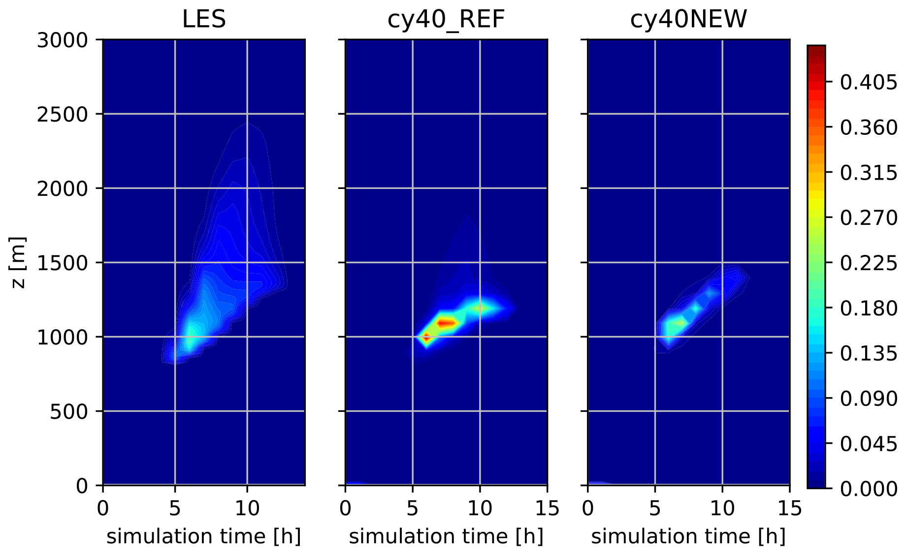
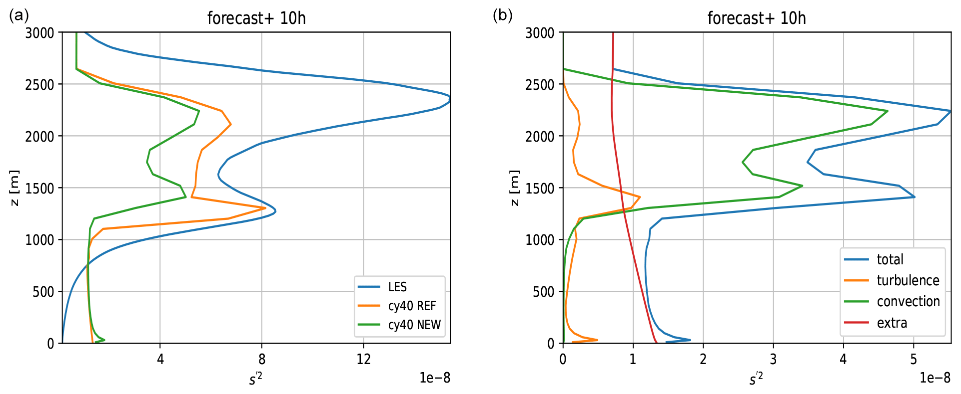
Figure 12 ARM case, 10th simulation hour. Panel (a) shows the profile of the variance in s in LES (blue), cy40REF (orange), and cy40NEW (green). Panel (b) shows the contribution of the turbulence (orange), convection (green), and the extra term (red) in Eq. (38) to the variance in s for cy40NEW.

Figure 13 ARM case, 10th simulation hour. The convective contribution to the variance in s of cy40NEW from the variance in θ_l (orange), total mixing ratio r_t (blue), and the covariance (green); see Eq. (21).

A closer examination of Figs. B1 and 5 reveals something remarkable: if we compare LES organised cloudy updraft transport (Fig. B1) with LES total turbulent transport (Fig. 5) in the upper part of the cloud layer, it becomes clear that organised transport alone would overestimate total transport in this region. If we look, e.g. at the +10 h forecast, LES shows almost no total turbulent transport above 2500 m despite considerable convective transport. To investigate this, we decompose the total turbulent transport in LES. Following Siebesma and Cuijpers (1995), total turbulent transport can be written as a sum of large-scale organised and small-scale subplume and environmental transport. In Appendix C, we elaborate on the nature of the turbulent transport in the upper part of the cloud layer by examining decomposed terms of the turbulent transport. This examination reveals that the rather good approximation of the total turbulent transport in the upper part of the cloud layer by the parameterisation seems to be the result of a compensation error in the ARM case; too-shallow mass flux transport is balanced by neglecting downward environmental turbulence (see Appendix C).

Additionally, the decomposition is used to look specifically into the turbulent transport around the cloud base inversion height in relation to the energy cascade term (Eq. 18); see Fig. 8. As shown in Fig. 8a, the LES θ_l profile around 1000 m height and after nine simulation hours is roughly the stable lapse rate (without phase changes) of the cloud layer. Considering this atmospheric stability, a standard turbulence scheme would provide little mixing at this level and higher. However, Fig. 8b reveals that the total turbulent transport is actually dominated by (small-scale) diffusive environmental turbulence up to considerably above the inversion height (in agreement with Fig. 7a and b in Siebesma and Cuijpers (1995) for the BOMEX shallow convection case). A plausible explanation for the presence of diffusive transport despite the stable conditions is (dry) updrafts terminating around the inversion height, in this way feeding the energy cascade from larger to smaller scales. Figure 5 for the ninth hour confirms that the dry updraft turbulent transport decreases strongly between 1000 and 1300 m height. This roughly corresponds to the layer with substantial diffusive environmental turbulent transport in LES despite the strong inversion (Fig. 8). If we compare the eddy diffusivity (ED) turbulent transport in the model versions, we see a clear increase from cy40REF without the 50⋅M_moist term (see Sect. 2.3), to cy40REF, to cy40NEW, which includes the energy cascade term (Fig. 9). In addition, organised entrainment at cloud base height (de Rooy and Siebesma, 2010) induced by acceleration of the moist updraft might further enhance small-scale environmental turbulence in this area. To describe the important contributions to the transport from subcloud-to-cloud layer as discussed above, the energy cascade term (Eq. 18) is added (Sect. 2.3).

Based on this shallow cumulus case, it is evident that the physical basis of our parameterisation is a strong simplification of reality. Moreover, the rather good approximation of the total turbulent transport during the ARM case is partly caused by a compensating error (Appendix C). However, a realistic representation would require a substantial increase in complexity, introducing new uncertain, tuneable parameters. Moreover, the current set of parameterisations performs well on a wide variety of cases.

3.1.2 Cloud cover

A contour plot of cloud fraction during the ARM case (Fig. 10) reveals that cy40 NEW results in lower maximum cloud fraction (near cloud base) in better correspondence with LES. This is also reflected in reduced total cloud cover (Fig. 11). Figure 11 further reveals that observed maximum total cloud cover is higher than in LES and peaks earlier. Brown et al. (2002) argues that the difference in timing between model results and observations is caused by differences between the initial profiles as prescribed in the case setup and the observations.

Observed differences in cloud fraction and cover between cy40REF and cy40NEW (Figs. 10 and 11, respectively) are the accumulated result of several modifications:

• As illustrated in Figs. 6 and 7, the reference configuration underestimates ventilation of the boundary layer leading to too-high humidity values near cloud base and therefore too-high maximum cloud fraction values. Especially the energy cascade (Eq. 18) is responsible for the enhanced ventilation (Sect. 3.1.1).

• Humidity near cloud base is also influenced by the dry updraft. In the reference formulation, Eq. (9) with a₂=40, entrainment, and therewith dilution of the updraft, remains rather small approaching the inversion. When this dry updraft finally terminates, relatively high amounts of moisture are detrained in the environment in cy40REF. With a₂=1 m, as in cy40NEW, this effect is mitigated.

• Another contribution to the different results stems from the removal of bugs in the reference cloud scheme. Most notable are erroneous thermodynamic coefficient β in Tudor and Mallardel (2004) and double application of a factor of 2 on the contribution to the variance by convection (Appendix A2). Especially the latter bug in cy40REF leads to a substantial increase in variance and accordingly to higher cloud fraction at cloud base.

• The largest impact is related to the choice of parameter c_ab (Sect. 2.4 Eq. 26 and Appendix A2). If c_ab=1 from cy40REF would be applied in the new configuration, the variance, and with it the cloud cover, would be substantially overestimated as demonstrated in Fig. 11. Only in cy40NEW is c_ab in line with literature (Redelsperger and Sommeria, 1981), i.e. 0.139.

Apart from the (too)-high cloud fractions at cloud base, also the underestimation of low values of cloud fraction in the upper part of the cloud layer by both model versions stands out in Fig. 10. Because the humidity (see Fig. 7) and temperature (not shown) profiles of cy40NEW closely match LES, the underestimation of cloud fraction in the upper part of the cloud layer must be related to an underestimation of variance in s. Figure 12a (for a typical hour) indeed reveals that both model versions underestimate the variance in s in the cloud layer, although cy40REF values are closer to LES. While the new configuration generally improves the shape of the variance profile, the local maximum near cloud top should be more pronounced. Note that inclusion of the convective covariance term, $\stackrel{\mathrm{‾}}{r_{\mathrm{t}}^{\prime }{\mathit{\theta }}_{\mathrm{l}}^{\prime }}$, helps to increase the local maximum near cloud top (Fig. 13).

Figure 12b clearly demonstrates that the contribution of convection to the variance in s is essential to adequately describe the shape of the variance profile in the cloud layer, especially the maximum near cloud top. Furthermore, it was decided not to include the contribution of the dry updraft to variance. First of all, together with the extra variance term (Sect. 2.4, Eq. 38, Fig. 12b), variance in the lower half of the subcloud layer would be too high. Moreover, with fluctuations in the termination level of the dry updraft, cloud cover near cloud base height changes, which can lead to noisy cloud cover patterns (not shown).

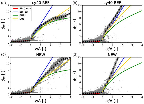
Figure 14 Dimensionless gradients of wind (a, c) and temperature (b, d) as a function of the local stability parameter $\frac{z}{\mathrm{\Lambda }}$ as diagnosed from 1 year of SCM output (grey dots). Panels (a, b) and (c, d) show the results for cy40REF and cy40NEW, respectively. Black dots represent the mean of the modelled dimensionless gradients. Blue lines indicate $\mathrm{1}+\mathrm{5}\frac{z}{\mathrm{\Lambda }}$ (Dyer, 1974); green lines (Beljaars and Holtslag, 1991) and yellow lines the relations proposed by Duynkerke (1991). Explanations of the different formulations can be found in the text. For completeness, Dyer (1974) formulations for unstable conditions are plotted (red line).

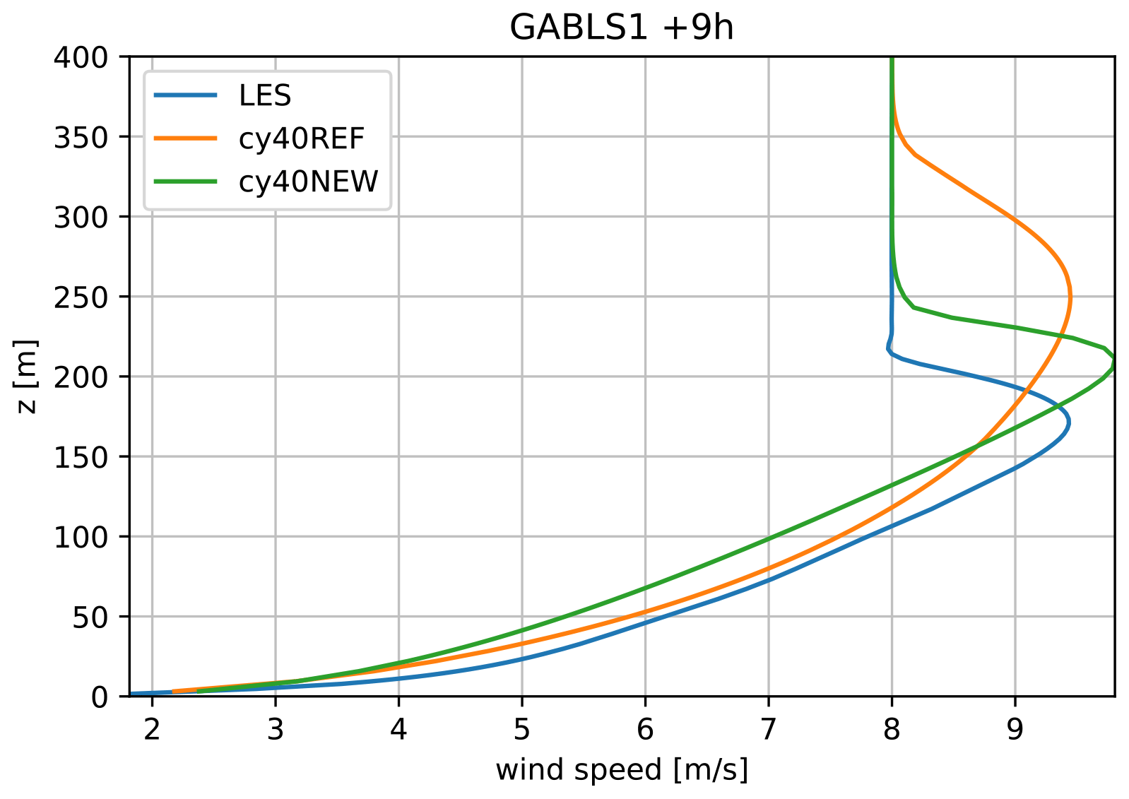
Figure 15 GABLS1 wind profile at the ninth simulation hour of LES model DALES (blue), cy40REF (orange), and cy40NEW (green). SCM runs use 64 levels with the lowest and highest model levels at 3 and 403 m, respectively. Note that results for GABLS1 with several LES models in Beare et al. (2006) reveal a spread in the height of the wind maximum, ranging from 175 to 200 m. The latter height and the corresponding LES profile in Beare et al. (2006) correspond well with cy40NEW.

Although the cloud scheme of cy40NEW already performs satisfactorily for a wide variety of weather conditions, there are clearly several options for further optimisation. Examples of possible improvement are the introduction of a height dependence of the extra variance term, partial replacement of the extra variance term by a dry updraft contribution in the subcloud layer, increasing τ_conv (Eq. 31) because the current value (Soares et al., 2004) seems to be on the low side (compare to, e.g. Siebesma et al., 2003), or modifying the energy cascade function (Eq. 19) to increase the local maximum around cloud top. An alternative way to address the underestimation of low cloud fraction values in the upper part of the cloud layer is the use of a skewed PDF (see, e.g. Bougeault, 1981), but this is not investigated here. Nevertheless, with a more sound physical basis and the removal of bugs, the new cloud scheme setup is already better suited as a base for such new developments.

3.2 Optimising the turbulence scheme

Two important modifications in the turbulence scheme are based on an evaluation procedure as described by Baas et al. (2008) and Baas et al. (2017). They demonstrated that a comparison of the dimensionless gradients of heat, ϕ_h, and momentum, ϕ_m, versus the stability parameter, $\frac{z}{\mathrm{\Lambda }}$ (Eq. 39), enables a more physically based choice of turbulence parameter settings for stable conditions.

$$\begin{array}{}\text{(39)}& {\displaystyle \frac{z}{\mathrm{\Lambda }}}={\displaystyle \frac{-\mathit{\kappa }z\frac{g}{{\mathit{\theta }}_{\mathrm{v}}}\stackrel{\mathrm{‾}}{w^{\prime }{\mathit{\theta }}_{\mathrm{v}}^{\prime }}}{u_{*}^{\mathrm{3}}}},\end{array}$$

where Λ is the local Obukhov length and u_* is the friction velocity. According to similarity theory there should be a universal relation between the dimensionless gradients and the stability parameter, although the uncertainty in these relations increases for stronger stratification, i.e. larger $\frac{z}{\mathrm{\Lambda }}$ values.

To investigate the mixing characteristics of our turbulence scheme in terms of the similarity relations, a SCM of HARMONIE-AROME is run for 1 year at the location of super-observation site Cabauw (Bosveld et al., 2020). The SCM is forced by output from daily three-dimensional forecasts of RACMO (van Meijgaard et al., 2008). The host model provides the advection and the initialisation of the surface. Every day at 12:00 UTC, the SCM produces a 72 h forecast with an interactive surface scheme. The SCM uses the same vertical resolution as the operational 3-D model, i.e. 65 layers with the lowest model level at approximately 12 m. Figure 14 shows the 1-year SCM output diagnosed in terms of flux–gradient relations for momentum and heat. We present results with default cy40REF settings; i.e. p=1 (Eq. 15) and c_h=0.15 (Eq. 14) next to p=2 and c_h=0.11 conform cy40NEW (see Sect. 2.3). Evaluation is restricted to stable boundary layer regimes, i.e. positive values of $\frac{z}{\mathrm{\Lambda }}$. Apart from model results, also theoretical relations according to Dyer (1974) in blue and Beljaars and Holtslag (1991) (green) and Duynkerke (1991) (yellow) are plotted. Many observational studies on flux–gradient relations report that for increasing stability the exchange of momentum is far more efficient than the exchange of heat, i.e. ϕ_h>ϕ_m (see, e.g. Beljaars and Holtslag, 1991). The relationship of Dyer (1974) does not reflect this and we focus on the relations of Beljaars and Holtslag (1991) and Duynkerke (1991) that were both derived from Cabauw observations. The divergence between the latter two flux–gradient relations for increasing stability illustrates the uncertainty under very stable conditions (Baas et al., 2008). Therefore, most attention is paid to neutral to moderately stable regimes, roughly corresponding with $\mathrm{0}<\frac{z}{\mathrm{\Lambda }}<\mathrm{1}$. Figure 14 shows that in this stability range, the reference setup underestimates mixing (overestimates the gradient) which can be related to linear interpolation between the length scales; i.e. p=1. However, only changing interpolation to quadratic would lead to excessive mixing and unrealistic flux–gradient relations (not shown). This can be compensated by reducing the proportionality factor of the stable length scale, c_h to 0.11. The combined result of these changes is shown in Fig. 14, where the lower panels reveal a better correspondence with the flux–gradient relations in near-neutral to moderately stable conditions. For more stable conditions, agreement with theoretical relations seems to deteriorate with the new setup. However, as explained above, the flux–gradient relations become highly uncertain under these strongly stratified conditions. To explore the performance of the turbulence scheme in moderately stable conditions, cy40REF and cy40NEW are compared to LES for the GABLS1 case (Beare et al., 2006), based on arctic observations. Although the change from p=1 to p=2 in the turbulence scheme (Sect. 2.3, Eq. 15) leads to increased mixing in near-neutral to weakly stable conditions, most other modifications, that reduce mixing (see Sect. 2.3), dominate for more stable conditions (see also Fig. 14). Results for GABLS1 (Fig. 15), showing the wind speed profile after 9 h of simulation, indeed reveal more stable profiles and lower boundary layer heights with cy40NEW, in better correspondence with LES.

Due to increased mixing in near-neutral conditions with p=2, the updates in HARATU to increase momentum mixing in strong wind conditions (see B17) are removed. Removing these updates together with the reduced c_h coefficient, overall decreases mixing at higher altitudes and therewith atmospheric inversions are better preserved. A similar impact stems from the last modification to the turbulence scheme we describe, decreasing the limiter on the minimum length scale, l_∞, from 100 to 40 (Sect. 2.3, Eq. 16). The exact value of l_∞ is highly uncertain, but also this parameter, active at higher altitudes, influences atmospheric inversion strengths. As demonstrated in the next sections, many of the improvements with cy40NEW arise from a more realistic representation of atmospheric inversions. In the next two sections, we demonstrate the impact of the modifications on low clouds and low cloud base heights.

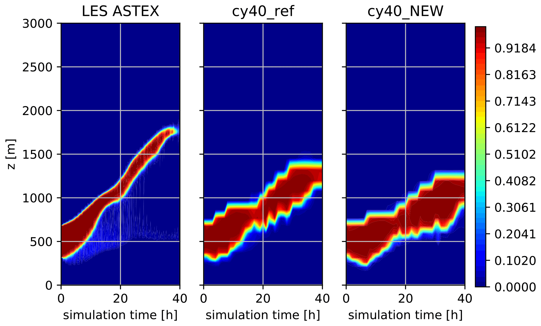
Figure 16 Cloud cover ASTEX case of LES (left panel), cy40REF (middle panel), and cy40NEW (right panel).

Figure 17 As Fig. 16 but for the slow case.

Figure 18 As Fig. 16 but for the fast case.

3.3 Stratocumulus-to-cumulus transition cases

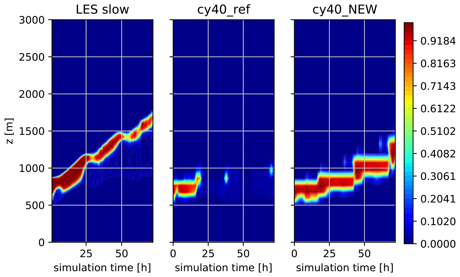
Figures 16, 17, and 18 show the results of three stratocumulus cases (see de Roode et al., 2016; Neggers et al., 2017). Whereas ASTEX is based on observations, the slow and fast cases are composite, idealised cases. LES results are obtained with DALES (de Roode et al., 2016). SCM runs are performed with 80 vertical layers (slightly higher resolution than operational), with the lowest layer at approximately 10 m. SCM results for ASTEX are rather comparable, although the new setup shows a slightly thicker and less rising cloud layer, less in agreement with LES. Note that the lower vertical resolution in SCMs compared to LES will usually lead to a more gradually rising cloud layer (Neggers et al., 2017). The slow and fast cases (differentiated by the speed of the low-level cloud transition), however, illustrate the trouble of cy40REF to maintain a stratocumulus layer, consistent with the strong underestimation of low clouds we see in operational practice. The improved results with the new setup are related to the accumulated effect of several modifications. As a result of a more efficient moisture transport towards the inversion in combination with a decreased transport through the inversion (better preservation of the inversion strength), more moisture is accumulated beneath the inversion, visible as a continuous and rising stratocumulus layer in the cy40NEW runs (Figs. 17 and 18).

There is one specific difference between the model versions we need to mention concerning the slow case. In the results for this case, only a moist updraft (see right panel of Fig. 4 in B17) was invoked in cy40REF because the bulk difference in potential temperature between the surface and 700 hPa exceeds the threshold of 20 ^∘C. The convective mixing with only a moist updraft in cy40REF is unable to transport enough moisture to the inversion. Even when the temperature inversion between surface and 700 hPa exceeds 20 ^∘C, it still seems legitimate to presume the existence of an ensemble of relatively weak, dry updrafts and stronger, moist updrafts. Moreover, rigid and rather arbitrary thresholds in parameterisations, like the above-mentioned bulk temperature difference, should be avoided (Kähnert et al., 2021). Based on the considerations above, the removal of the stratocumulus regime with only a wet updraft is part of the cy40NEW configuration and therefore applies to all results of cy40NEW in this paper.

3.4 HARMONIE-AROME 3-D model runs

As mentioned in Sect. 1, the most urgent problem in cy40REF concerns the large underestimation of low clouds and overestimation of cloud base heights (i.e. the lowest model level where cloud fraction exceeds $\frac{\mathrm{5}}{\mathrm{8}}$). This model deficiency is most noticeable in wintertime conditions. As a typical example, we show 3-D model results for 19 December 2018 in Fig. 19. The cy40REF run reveals a severe overestimation of cloud base height. Moreover, for large areas with observed low stratus, cloud base height is not even detected due to too-small cloud fractions (shown as white, background colour). A key aspect of the large improvement with cy40NEW (Fig. 19, right panel) is again the better preservation of inversion strengths. Several modifications contribute to the improvement but the most substantial is the influence of reduced l_∞ (see Eq. 16) and c_h (Eq. 14) as well as removal of the HARATU updates, increasing the downward mixing described in B17 (see also Sect. 3.2). The large improvement on cloud base height is confirmed in longer-term verification, illustrated by the frequency bias for December 2018 (Fig. 20). Here, frequency bias means the ratio between the forecasted and observed number of cloud base heights in a certain bin. Note the extreme underestimation of cloud bases around 178 ft (approximately 54 m); less than 20 % of the observed number of cases are actually predicted in +24 h cy40REF forecasts. Over the complete range of low cloud base heights, cy40NEW outperforms cy40REF, except for the lowest cloud base, associated with fog cases. However, in fog, other processes (concerning microphysics and radiation) outside the scope of this study turn out to have a large influence. Verification for other months confirms the substantial improvement in low cloud base height climatology.

Figure 19 Cloud base height in feet (1 ft is 0.3048 m) on 19 December 2018 at 09:00 UTC as measured at discrete observation site locations in the Netherlands and part of the North Sea (left panel), forecasted by cy40REF (middle panel) and cy40NEW (right panel). Note that white in the left panel means that there is no observation available, whereas white spots in the middle and right panels mean no cloud base height was detected because all model levels have a cloud fraction $<\frac{\mathrm{5}}{\mathrm{8}}$.

Figure 20 Frequency bias of the cloud base height in feet (1 ft is 0.3048 m) for December 2018 with cy40REF (a) and cy40NEW (b). Blue, green, and orange lines refer to +3, +24, and +48 h forecasts, respectively.

Apart from the impact on low clouds, the accumulation of moisture beneath atmospheric inversions also influences the triggering of resolved deep convection and the associated (heavy) precipitation. This is illustrated in Fig. 21, which presents a case on 10 September 2011 where deep convection was observed but its triggering was missed by cy40REF. The vertical atmospheric cross sections in Fig. 21 (third and fourth rows) reveal that relative humidity just under the inversion of the boundary layer accumulates more strongly in cy40NEW. This supports the model to start resolved upward motions as reflected in the increased boundary layer height near the local maximum in RH at the boundary layer top (fourth row, third column). As a result, only in cy40NEW, deep, resolved convection and precipitation starts (noisy pattern in the upper right corner of the fourth row and column). Figure 22, showing the averaged skewed temperature profile in the area where the deep convective shower develops (indicated by the rectangle in Fig. 21), confirms the stronger atmospheric inversion with cy40NEW.

Semi-operational, daily runs of cy40REF and cy40NEW for more than a year in parallel revealed several cases where cy40NEW did forecast resolved precipitation that was also observed but was missed in cy40REF. Moreover, 1 year of fraction skill score verification of precipitation forecasts against calibrated radar data demonstrated a significant improvement with cy40NEW (not shown). Verification of the near-surface variables reveals that the new configuration results in a slight deterioration in the negative 2 m temperature bias but no significant impact on 2 m humidity. Wind speeds at 10 m are slightly higher but with the same diurnal amplitude, resulting in no significant change in model performance. Note that in general, near-surface variables are strongly influenced by surface processes and potential representation mismatches between observation site and model grid box (see, e.g. de Rooy and Kok, 2004).

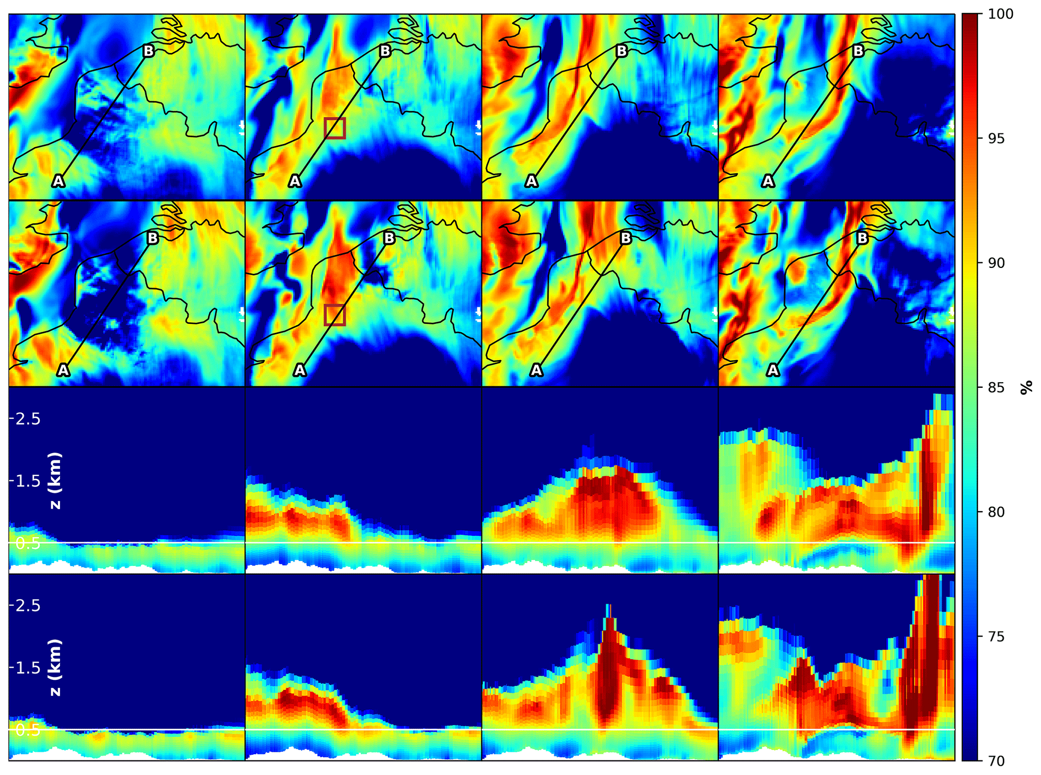
Figure 21 Relative humidity (RH) plots (red means high RH, blue low RH) for 10 September 2011. The four columns refer to hours 12:00, 14:00, 16:00, and 18:00 UTC. The first row (cy40REF) and second row (cy40NEW) show a map of RH at approximately 500 m height that covers parts of Belgium and northwest France, as well as a black line. Along this line, a vertical atmospheric cross section for the lowest 3 km is shown in the third (cy40REF) and fourth (cy40NEW) rows. In the cross sections, the boundary layer can be recognised by relatively high RH values. The white line at 500 m in the cross sections shows the height for which the RH is plotted in the two upper rows. The rectangle in the second column of the two upper rows indicates the area used to produce the skewed T profile in Fig. 22.

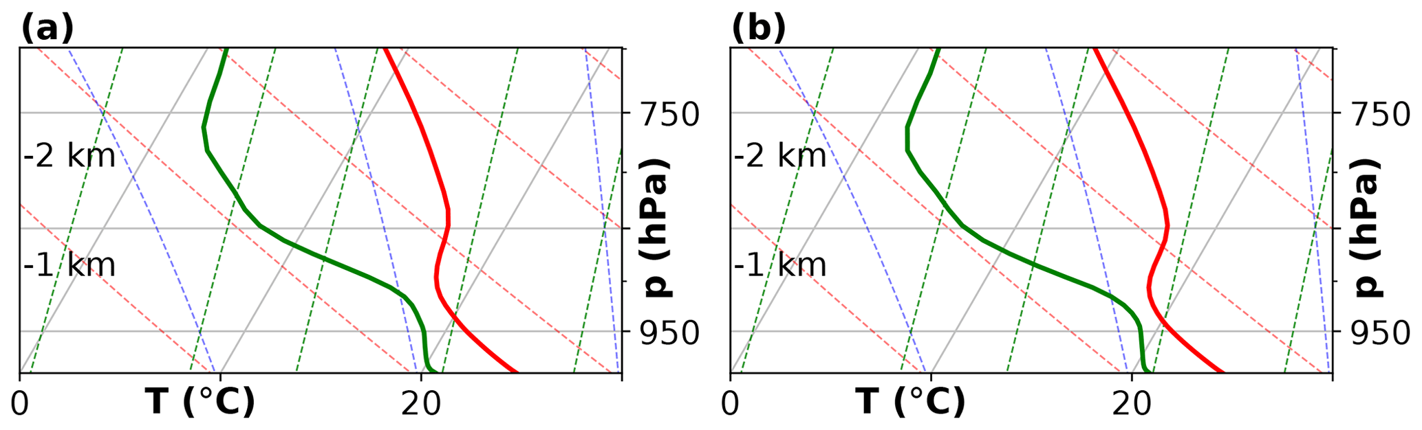
Figure 22 Profiles of the skewed temperature (solid red line) and dew point temperature (solid green line) against the pressure (hPa). The profiles for cy40REF (a) and cy40NEW (b) are determined as the average over the domain indicated by the rectangle in Fig. 21, where a strong shower did develop in cy40NEW but not in cy40REF. Dashed red, blue, and green lines show, respectively, the dry adiabat, the pseudo adiabat, and constant mixing ratio. Skewed thin grey lines represent constant temperature. In comparison with cy40REF, cy40NEW reveals a stronger inversion around the top of the boundary layer (approximately 1000 m height).

4 Conclusions and discussion

As discussed in, e.g. Jakob (2010) or de Rooy et al. (2013), model development, in particular by means of improved parameterisation schemes, is a slow and sometimes frustrating process. A scientifically improved parameterisation could remove a previous compensating model error and consequently cause an overall deterioration. In addition, together with increased physical realism, interactions between parameterisations become stronger. The considerations above advocate a more integral approach to develop strongly connected parameterisation schemes together. Following such an approach, this paper describes a comprehensive model update to the boundary layer schemes. Because the involved parameterisations are all built on widely applied frameworks, the here-described modifications and the impact of certain parameters on different model aspects are not just specific to the HARMONIE-AROME model but also applicable to many NWP and climate models. Moreover, this paper can be an inspiration for further improvements, and several suggestions for this are already provided, for example, amelioration of the variance in s estimates by increasing the convection timescale, τ_conv (Eq. 31), or including a height dependency in the extra variance term, Eq. (38).

Apart from being a slow and tough process, model development is often a compromise between a scientific and a pragmatic approach. In this paper, we have tried to provide an “honest” description of the development process, thus including the more pragmatic optimisations and mentioning not only the successes but also the remaining shortcomings and (over)simplifications in the parameterisations.

The model update contains substantial modifications to the cloud, turbulence, and convection schemes based on a wide variety of argumentations. On one side of the spectrum are the more theoretically based modifications to the turbulence scheme – Monin–Obukhov similarity theory, following Baas et al. (2008) and Baas et al. (2017) – and the statistical cloud scheme (fundamental thermodynamics). On the other end of the spectrum, this paper illustrates that parameterisations contain uncertain parameters, with largely varying values suggested in the literature, that at the same time have a substantial impact. To optimise these parameters, we inevitably have to rely on examination of cases and longer term 3-D runs. Finally, LES and SCM runs conducted for a variety of intercomparison cases have been analysed extensively and the outcomes are subsequently used as a basis for several modifications in all boundary layer schemes. As an example, we mention the incorporation of the lateral mixing term from the prognostic mass flux vertical velocity variance equation as a source term in the TKE equation. This term is related to the energy cascade from large to smaller scales and particularly enhances the subcloud-to-cloud layer transport improving the correspondence with LES results for shallow convection. An overview of all modifications is provided in Table D1.

The adjustments to the HARMONIE-AROME model described in this paper have a substantial impact on several aspects of the model performance. The most outstanding result is the improvement on low cloud and low cloud base height forecasts. Being one of the most urgent deficiencies of HARMONIE-AROME cycle 40, increasing the quality on this aspect was also the main goal of this study. The low cloud climatology changes from a severe underestimation in the reference version to a well-balanced model. Obviously, low clouds have a large impact on radiation and therewith on several model parameters. Moreover, they are crucial for aviation safety purposes. Taking a closer look at the consequences of the model updates reveals that the better preservation of atmospheric inversion strengths plays a key role. Not only the formation of low clouds but also the triggering of deep-resolved convection and the associated (heavy) precipitation are influenced by atmospheric inversion strength. With stronger inversions, more humidity is accumulated beneath the boundary layer top, which supports the development of mesoscale resolved upward motions, ultimately leading to deep convection and rain showers.

Verification based on more than 1 year of parallel model runs with cy40REF and cy40NEW firmly substantiates the significant improvement on low cloud and precipitation forecasts. The modifications in cy40NEW did not result in a significant improvement or deterioration of near-surface temperature, humidity, and wind speed. All modifications have recently been incorporated in the default configuration of HARMONIE-AROME cycle 43. Herewith, they will also become available in the HARMONIE-AROME climate version (Belus̆ić et al., 2020) undoubtedly with impact on, e.g. precipitation extremes in future weather experiments.

An important spin-off of this project is the increased understanding of how parameter settings impact particular model output and how they influence each other via underlying physical processes. With this insight, we decided to use the proportionality constant of the stable length scale, c_m,h (Eq. 14) and the minimum asymptotic length scale, l_∞ (Eq. 16) within a SPP (stochastically perturbed parameterisation) EPS framework (Frogner et al., 2019). Verification reveals that these parameters have the most beneficial impact on spread/skill of all parameters investigated (Inger-Lise Frogner, personal communication, 2021​​​​​​​).

Appendix A

A1 Derivation of the variance in s

Here, we provide a step-by-step derivation of the variance in s.

Suppose we know the PDF that describes subgrid variability of θ_l and q_t in a grid box of an atmospheric model. Then the resulting cloud cover, a_c, and liquid water content (similarly for ice water content) can be written as

$$\begin{array}{}\text{(A1)}& \begin{array}{rl}& a_{\mathrm{c}}=\underset{-\mathrm{\infty }}{\overset{\mathrm{\infty }}{\int }}H(q_{\mathrm{t}}-q_{\mathrm{s}})P({\mathit{\theta }}_{\mathrm{l}},q_{\mathrm{t}})\mathrm{d}{q}_{\mathrm{t}}\mathrm{d}{\mathit{\theta }}_{\mathrm{l}}\\ & q_{\mathrm{l}}=\underset{-\mathrm{\infty }}{\overset{\mathrm{\infty }}{\int }}(q_{\mathrm{t}}-q_{\mathrm{s}})H(q_{\mathrm{t}}-q_{\mathrm{s}})P({\mathit{\theta }}_{\mathrm{l}},q_{\mathrm{t}})\mathrm{d}{q}_{\mathrm{t}}\mathrm{d}{\mathit{\theta }}_{\mathrm{l}},\end{array}\end{array}$$

where q_s is the saturation specific humidity and H denotes the Heaviside function (H(x)=0 for x<0 and H(x)=1 for x>0) which probes that part of the integrand that is oversaturated. Because we only have to consider $q_{\mathrm{t}}-q_{\mathrm{s}}>\mathrm{0}$, the distance to the saturation curve s can be defined as

$$\begin{array}{}\text{(A2)}& s\equiv \stackrel{\mathrm{‾}}{s}+s^{\prime }=q_{\mathrm{t}}-q_{\mathrm{s}}(p,T)=q_{\mathrm{l}}\text{for}s>\mathrm{0},\end{array}$$

where $\stackrel{\mathrm{‾}}{s}$ is the (grid box) average of s, primes denote excursions from the mean, and q_s is a function of pressure, p, and temperature T. Using a Taylor expansion around $\stackrel{\mathrm{‾}}{T_{\mathrm{l}}}$, the saturation specific humidity at T can be written as

$$\begin{array}{}\text{(A3)}& q_{\mathrm{s}}\left(T\right)\simeq {\stackrel{\mathrm{‾}}{q}}_{\mathrm{sl}}+{\stackrel{\mathrm{‾}}{q}}_{\mathrm{sl},\mathrm{T}}(T-{\stackrel{\mathrm{‾}}{T}}_{\mathrm{l}}),\end{array}$$

with the usual abbreviations:

$$\begin{array}{}\text{(A4)}& {\stackrel{\mathrm{‾}}{q}}_{\mathrm{sl}}=q_{\mathrm{s}}\left({\stackrel{\mathrm{‾}}{T}}_{\mathrm{l}}\right),{\stackrel{\mathrm{‾}}{q}}_{\mathrm{sl},\mathrm{T}}={\displaystyle \frac{\partial q_{\mathrm{s}}\left({\stackrel{\mathrm{‾}}{T}}_{\mathrm{l}}\right)}{\partial T}},\end{array}$$

using the definition of the liquid water temperature:

$$\begin{array}{}\text{(A5)}& T_{\mathrm{l}}\equiv T-{\displaystyle \frac{L}{c_{\mathrm{p}}}}{q}_{\mathrm{l}},\end{array}$$

where L is the latent heat of vaporisation and c_p the heat capacity of dry air at constant pressure. Equation (A3) can be rewritten as

$$\begin{array}{}\text{(A6)}& \begin{array}{rl}{q}_{\mathrm{s}}\left(T\right)& \simeq {\stackrel{\mathrm{‾}}{q}}_{\mathrm{sl}}+{\stackrel{\mathrm{‾}}{q}}_{\mathrm{sl},\mathrm{T}}(T_{\mathrm{l}}+{\displaystyle \frac{L}{c_{\mathrm{p}}}}{q}_{\mathrm{l}}-{\stackrel{\mathrm{‾}}{T}}_{\mathrm{l}})={\stackrel{\mathrm{‾}}{q}}_{\mathrm{sl}}+{\stackrel{\mathrm{‾}}{q}}_{\mathrm{sl},\mathrm{T}}\\ & \times \left(\mathit{\pi }{\mathit{\theta }}_{\mathrm{l}}^{\prime }+{\displaystyle \frac{L}{c_{\mathrm{p}}}}H\left(s\right)s\right),\end{array}\end{array}$$

where we have applied Eq. (A2) and the Exner function, $\mathit{\pi }=(\frac{p}{p_{\mathrm{0}}}{)}^{\frac{R_{\mathrm{d}}}{c_{\mathrm{p}}}}=\frac{T}{\mathit{\theta }}$, with R_d the gas constant of dry air and p₀ a reference surface pressure. Equation (A6) substituted in Eq. (A2) leads to

$$\begin{array}{}\text{(A7)}& s={\stackrel{\mathrm{‾}}{q}}_{\mathrm{t}}+q_{\mathrm{t}}^{\prime }-{\stackrel{\mathrm{‾}}{q}}_{\mathrm{sl}}-q_{\mathrm{sl},\mathrm{T}}\mathit{\pi }{\mathit{\theta }}_{\mathrm{l}}^{\prime }-q_{\mathrm{sl},\mathrm{T}}{\displaystyle \frac{L}{c_{\mathrm{p}}}}H\left(s\right)s.\end{array}$$

As mentioned before, we only consider s>0, so H(s)=1. Writing s explicitly in Eq. (A7) leads to

$$\begin{array}{}\text{(A8)}& s=\mathit{\alpha }[q_{\mathrm{t}}^{\prime }-\mathit{\beta }{\mathit{\theta }}_{\mathrm{l}}^{\prime }+({\stackrel{\mathrm{‾}}{q}}_{\mathrm{t}}-{\stackrel{\mathrm{‾}}{q}}_{\mathrm{sl}}\left)\right],\end{array}$$

with α and β defined in Eq. (22). To determine s^′, we follow a similar derivation as shown above but now for $\stackrel{\mathrm{‾}}{s}$.

$$\begin{array}{}\text{(A9)}& {\displaystyle }\stackrel{\mathrm{‾}}{s}={\stackrel{\mathrm{‾}}{q}}_{\mathrm{t}}-{\stackrel{\mathrm{‾}}{q}}_{\mathrm{s}}\left(\stackrel{\mathrm{‾}}{T}\right)\text{(A10)}& {\displaystyle }{\stackrel{\mathrm{‾}}{q}}_{\mathrm{s}}\left(\stackrel{\mathrm{‾}}{T}\right)\simeq {\stackrel{\mathrm{‾}}{q}}_{\mathrm{sl}}+{\stackrel{\mathrm{‾}}{q}}_{\mathrm{sl},\mathrm{T}}(\stackrel{\mathrm{‾}}{T}-{\stackrel{\mathrm{‾}}{T}}_{\mathrm{l}}),\end{array}$$

with $(\stackrel{\mathrm{‾}}{T}-{\stackrel{\mathrm{‾}}{T}}_{\mathrm{l}})=\frac{L}{c_{\mathrm{p}}}{\stackrel{\mathrm{‾}}{q}}_{\mathrm{l}}=\frac{L}{c_{\mathrm{p}}}\stackrel{\mathrm{‾}}{s}$ substituted in Eq. (A9), $\stackrel{\mathrm{‾}}{s}$ reads

$$\begin{array}{}\text{(A11)}& \stackrel{\mathrm{‾}}{s}=\mathit{\alpha }({\stackrel{\mathrm{‾}}{q}}_{\mathrm{t}}-{\stackrel{\mathrm{‾}}{q}}_{\mathrm{sl}}).\end{array}$$

Using Eqs. (A8) and (A11), we can write s^′ as

$$\begin{array}{}\text{(A12)}& s^{\prime }=s-\stackrel{\mathrm{‾}}{s}=\mathit{\alpha }{q}_{\mathrm{t}}^{\prime }-\mathit{\alpha }\mathit{\beta }{\mathit{\theta }}_{\mathrm{l}}^{\prime },\end{array}$$

and the variance of s as

$$\begin{array}{}\text{(A13)}& {\mathit{\sigma }}_{\mathrm{s}}^{\mathrm{2}}=\stackrel{\mathrm{‾}}{{s^{\prime }}^{\mathrm{2}}}={\mathit{\alpha }}^{\mathrm{2}}\stackrel{\mathrm{‾}}{{q_{\mathrm{t}}^{\prime }}^{\mathrm{2}}}-\mathrm{2}{\mathit{\alpha }}^{\mathrm{2}}\mathit{\beta }\stackrel{\mathrm{‾}}{q_{\mathrm{t}}^{\prime }{\mathit{\theta }}_{\mathrm{l}}^{\prime }}+{\mathit{\alpha }}^{\mathrm{2}}{\mathit{\beta }}^{\mathrm{2}}\stackrel{\mathrm{‾}}{{{\mathit{\theta }}_{\mathrm{l}}^{\prime }}^{\mathrm{2}}}.\end{array}$$

A2 Summary of the differences between the cy40REF and cy40NEW cloud schemes

Here we present an overview of the differences between the cy40REF and cy40NEW cloud schemes. Firstly, an important difference concerns the formulation of the thermodynamic coefficients α and β in the expression for the variance in s (Eq. 21). The definitions and derivation in cy40NEW can be found in the previous Appendix. In cy40REF, coefficient α is formulated as Eq. (22) except for a factor of 0.5 (see Tudor and Mallardel, 2004). Coefficient β in cy40REF is combined with α in one variable in a complex expression, described in Tudor and Mallardel (2004) but without a derivation or reference. The values and typical atmospheric shape of the profile of β in the original code are wrong, as they deviate substantially from Eq. (22) (not shown). Furthermore, in cy40REF, it is assumed that l_ϵ equals l_m (Eq. 30), whereas in the new configuration we take l_ϵ consistent with its formulation in the turbulence scheme (see Eq. 27). Pre-factor c_ab in Eq. (26) was 1 in cy40REF but changed to 0.139, this time conforming to the literature (Redelsperger and Sommeria, 1981). In contrast to the reference code, the new setup of the cloud scheme includes the covariance term of the contribution from convection, i.e. Eq. (31) with a=θ_l and b=q_t. Finally, pre-factor 2 of the variance contribution from convection (see, e.g. Eq. 32) was erroneously applied twice in cy40REF and removed in cy40NEW.

Appendix B: Modifications in the convection scheme

To estimate the contribution from organised (updraft) transport, in a model represented by the convection scheme, to the total turbulent transport, LES data in the cloud layer are conditionally sampled. Different sampling methods exist (see Siebesma and Cuijpers, 1995) like cloudy updraft sampling, i.e. selecting LES grid boxes with w_u>0 and q_l>0, and core sampling with the additional requirement of positive buoyancy. Cloudy updraft sampling is probably the most suitable to be compared with convective transport of a mass flux scheme because it includes the negatively buoyant, decelerating part of the updraft, just as in the parameterisation.

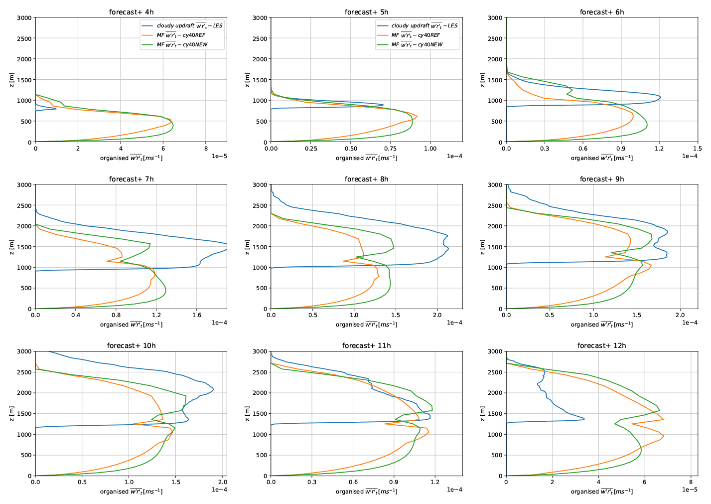
Figure B1 Kinematic convective transport (m s⁻¹) during all convective hours of the ARM case, corresponding to simulation hours +4 to +12 h. Plotted is the mass flux (MF) transport by the convection scheme (orange indicates cy40REF and green is cy40NEW) and the estimated (cloudy updraft sampling) convective transport by the LES (blue). Note that the x-axis scale is not constant and equal to the scale of the corresponding plots in Fig. 5

Figure B1 shows convective humidity transport according to LES (cloudy updraft sampling) and HARMONIE-AROME 1-D with the cy40REF and cy40NEW configurations. Plots of heat transport are not shown as they reveal a similar behaviour. The plotted HARMONIE-AROME values are the sum of dry and moist updraft transport, whereas the sampling method applied on the 3-D fields of LES will only produce estimates of convective transport in the cloud layer. To increase statistical significance, the model mass flux transport is obtained as hourly mean around validation time. From LES, only instantaneous hourly 3-D fields are available. However, as LES convective transport is the mean of 100 HARMONIE-sized domains, it can be considered an average over many realisations.

Figure B1 shows that during the main part of the convective period, both model versions underestimate convective transport in comparison with LES. Only during the last convective hours, fluxes are comparable, whereas at +12 h convection finally starts to collapse. The latter hour is highly dynamical and a slightly different (e.g. shorter) averaging time already has a large impact on the diagnosed flux profiles. Hence, +12 h results should be interpreted with care. Figure B1 further demonstrates that the new configuration increases convective transport, generally resulting in a better resemblance with LES. Several modifications in the convection scheme have contributed to this increase in mass flux transport. All modifications to the convection scheme, including their impact, are described below.

Firstly, we changed c_b in the mass flux closure (Eq. 12) from 0.03 (Grant, 2001) to 0.035 (Brown et al., 2002); see Sect. 2.2. Another contribution stems from the formulation of ε at z=z_lcl (Eq. 10, Sect. 2.2.1). In the original expression, entrainment at cloud base (or inversion height) is inversely proportional to the inversion height. With a typically increasing inversion height during the convective period, this formulation will result in relatively high entrainment rates and therewith less effective mass flux transport in the early stages of convection. However, during this period, the convective transport is underestimated (see Fig. B1). Therefore, we pragmatically fixed moist updraft entrainment values at cloud base at 0.002, roughly in agreement with LES in de Rooy et al. (2013), Fig. 6, and Siebesma et al. (2003). However, more investigation is needed to establish a robust and adequate description of the entrainment at cloud base. Another aspect of the entrainment formulations in cy40REF are the quite large values near the surface due to the first term on the RHS in Eqs. (9) and (10). Apart from unwanted dependence on vertical resolution of the model, this will also result in a weak dependence of updraft excess values on surface fluxes. By adding a₁=40 m to the entrainment formulations, similar to Soares et al. (2004), dependence on surface fluxes gets stronger, causing increased convective transport during hours with large surface fluxes (Brown et al., 2002, Fig. 3). Finally, a₂ in Eq. (9) is reduced from 40 to 1 m to increase entrainment values when the dry updraft approaches its termination height. Herewith, deposition of humidity in a too-thin layer just below the inversion is prevented, which contributes to the too-high humidity and cloud cover around cloud base in cy40REF (see Sect. 3.1.2).

Finally, Fig. B1 reveals a strong decrease in mass flux transport around inversion which is related to the termination height of the dry updraft (see Fig. 5) and the associated strong decrease of convective transport. However, as we demonstrate in Sect. 3.1.1, this decrease in convective transport is largely balanced by the diffusive transport leading to a rather smooth total turbulent transport profile (Fig. 5). This process is enhanced by the incorporation of the energy cascade term in the turbulence scheme (Sect. 2.3).

Appendix C: Decomposition of the turbulent transport

Following Siebesma and Cuijpers (1995), total turbulent transport can be written as a sum of large-scale organised and small-scale subplume and environmental transport. Figure C1 presents typical profiles during the ARM case of such a decomposition of total turbulent transport. The role of environmental turbulence in Fig. C1 is remarkable. In the lower half of the cloud layer, the negative contribution of environmental turbulence is roughly balanced by positive subplume turbulence. However, in the upper part of the cloud layer, a large negative contribution of environmental turbulence dominates and counteracts organised updraft transport. Consequently, the underestimation and too-shallow organised convective transport by the parameterisation (Fig. B1) are not translated in an underestimation of total turbulent transport (Fig. 5). Note that in Siebesma and Cuijpers (1995), Fig. 7 for the BOMEX steady-state shallow convection case, environmental turbulence is always positive. Their figure is produced by applying cloud core sampling. However, repeating the decomposition experiments with different sampling methods leads to the same qualitative picture.

To investigate the relatively large contribution from environmental turbulence, the turbulent transport is decomposed further in three parts: cloudy updraft, cloudy downdraft, and environment (Siebesma and Cuijpers, 1995). As a result, we now distinguish 6 different turbulent fluxes contributing to the total turbulent transport of moisture (Fig. C2). Figure C2 reveals that less than half of the negative turbulent transport is caused by organised downdrafts, whereas the majority is caused by environmental turbulence outside cloudy up- and downdrafts. To visualise the downward transport, a horizontal cross section is taken at the height of maximum downward turbulent moisture transport (Fig. C3). The largest downward transport (dark blue colour) is observed in two subdomains indicated by black squares and seems to be connected to strong upward transport. However, the two subdomains reveal a different behaviour (Figs. C3 middle and right panels). Whereas the right subdomain resembles the classical view with downward transport in the cloud (downdrafts), the left subdomain shows downward transport primarily outside the cloud (indicated by the red q_l=0 line), possibly the remains of a large active updraft. Here, a substantial part of downward transport is associated with downdrafts containing relatively high humidity values but no liquid water. Possibly, these downdrafts are related to the subsiding shells as discussed by Heus et al. (2009).

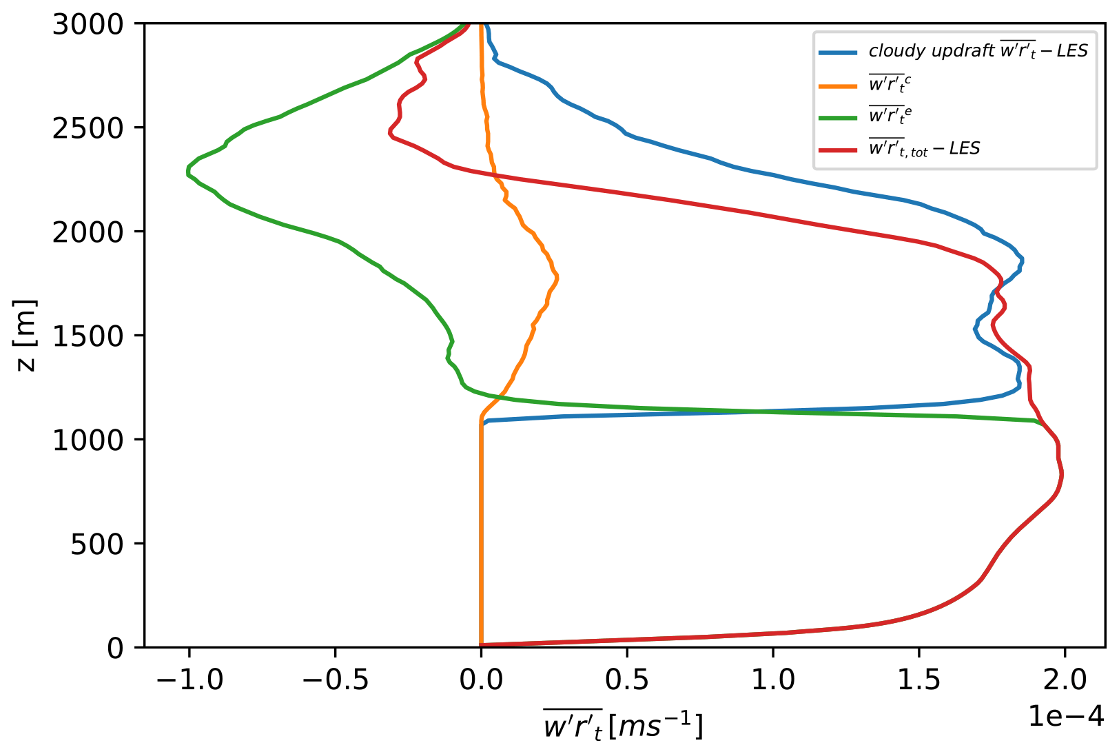
Figure C1 Decomposition of the turbulent fluxes for the ARM case, ninth simulation hour. Plotted are LES cloudy updraft flux (blue), small-scale subplume transport (orange), small-scale environmental transport (green), and total transport (red).

Finally, Fig. C3a illustrates that LES runs for the ARM case at a smaller domain could easily miss rarely occurring large convective events that give rise to substantial downward transport. As a result, investigations on smaller domain LES could lead to different conclusions about the relative importance of the decomposed fluxes to the total turbulent transport.

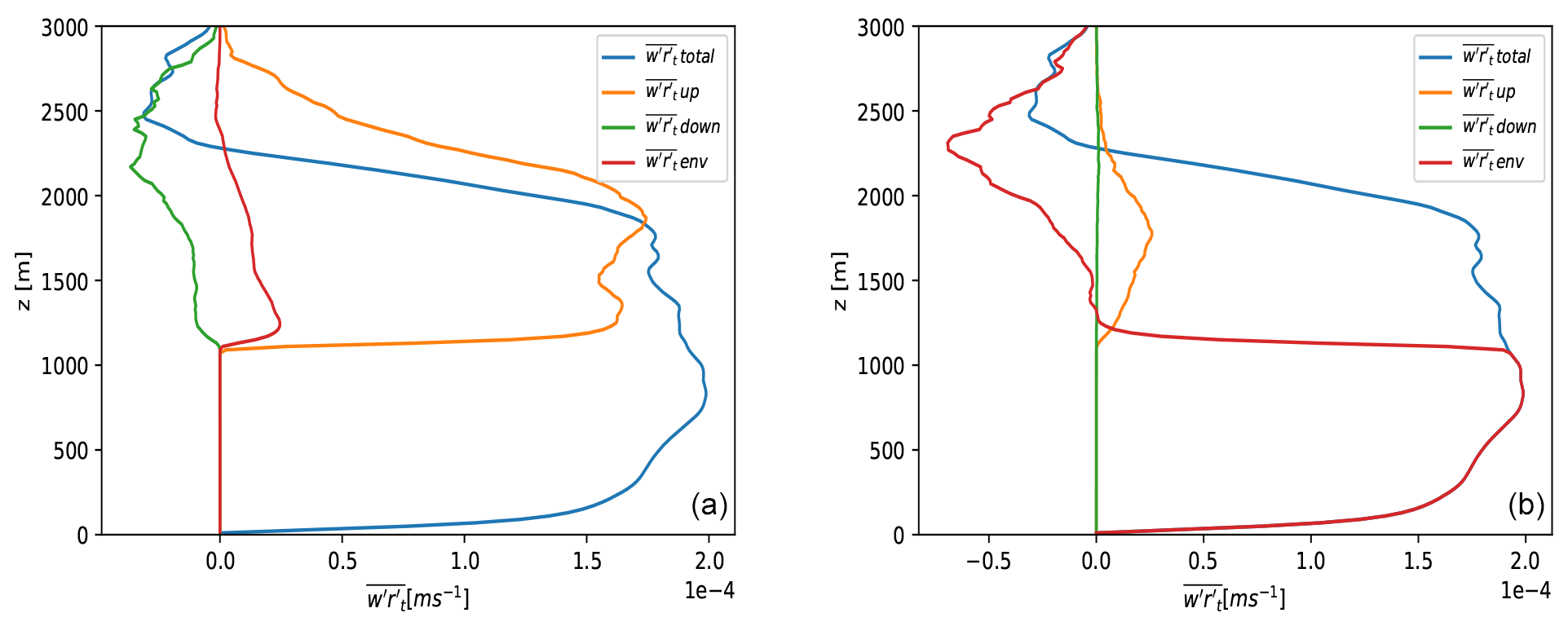
Figure C2 ARM case, ninth simulation hour. Panel (a) shows organised fluxes, distinguishing updrafts (orange), downdrafts (green), and environment (red) as well as the total turbulent transport (blue). Panel (b) shows the small-scale turbulent fluxes using similar colour coding to that in panel (a).​​​​​​​

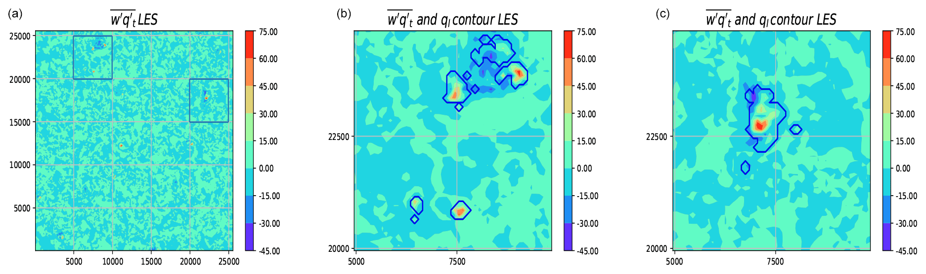
Figure C3 ARM case, ninth simulation hour, cross section of the kinematic turbulent moisture transport at 2310 m height (with q_t in g kg⁻¹). Blue and yellow/red colours refer to downward and upward transport, respectively. The x and y axes number the LES grid points (with the LES resolution of 100 m; the grey grid lines illustrate the size of a HARMONIE-AROME grid box). Panel (a) presents the full LES domain, whereas panels (b) and (c) show, respectively, the left and right subdomains as shown by the blue squares in panel (a). The blue line defines the cloudy border, i.e. q_l=0.

Appendix D: Overview of the modifications

Table D1