An improved regional coupled modeling system for Arctic sea ice simulation and prediction: a case study for 2018

The improved and updated Coupled Arctic Prediction System (CAPS) is evaluated using a set of Pan-Arctic prediction experiments for the year 2018. CAPS is built on the Weather Research and Forecasting model (WRF), the Regional Ocean Modeling System (ROMS), the Community Ice CodE (CICE), and a data assimilation based on the local error subspace transform Kalman filter. We analyze physical processes linking improved and changed physical parameterizations in WRF, ROMS, and CICE to changes in the simulated Arctic sea ice state. Our results show that the improved convection and boundary layer schemes in WRF result in an improved simulation of downward radiative fluxes and near-surface air temperature, which influences the predicted ice thickness. The changed tracer advection and vertical mixing schemes in ROMS reduce the bias in sea surface temperature and change ocean temperature and salinity structure in the surface layer, leading to improved evolution of the predicted ice extent (particularly correcting the late ice recovery issue in the previous CAPS). The improved sea ice thermodynamics in CICE have noticeable influences on the predicted ice thickness. The updated CAPS can better predict the evolution of Arctic sea ice during the melting season compared with its predecessor, though the prediction still has some biases at the regional scale. We further show that the updated CAPS can remain skillful beyond the melting season, which may have a potential value for stakeholders to make decisions for socioeconomic activities in the Arctic.

1 Introduction

Over the past few decades, the extent of Arctic sea ice has decreased rapidly and entered a thinner and younger regime associated with global climate change (e.g., Kwok, 2018; Serreze and Meier, 2019). The dramatic changes in the properties of Arctic sea ice have gained increasing attentions by a wide range of stakeholders, such as trans-Arctic shipping, natural resource exploration, and activities of coastal communities relying on sea ice (e.g., Newton et al., 2016). This leads to increasing demands on skillful Arctic sea ice prediction, particularly at seasonal timescales (e.g., Jung et al., 2016; Liu et al., 2019; Stroeve et al., 2014). However, Arctic sea ice predictions based on different approaches (e.g., statistical method and dynamical model) submitted to the Sea Ice Outlook, a community effort managed by the Sea Ice Prediction Network (SIPN, https://www.arcus.org/sipn, last access: 27 June 2021), show substantial biases in the predicted seasonal minimum of Arctic sea ice extent compared to the observations for most years since 2008 (Liu et al., 2019; Stroeve et al., 2014).

Recently, we have developed an atmosphere–ocean–sea ice regional coupled modeling system for seasonal Arctic sea ice prediction (Yang et al., 2020, hereafter Y20), in which the Community Ice CodE (CICE) is coupled with the Weather Research and Forecasting Model (WRF) and the Regional Ocean Modeling System (ROMS), hereafter called Coupled Arctic Prediction System (CAPS). To improve the accuracy of initial sea ice conditions, CAPS employs an ensemble-based data assimilation system to assimilate satellite-based sea ice observations. Seasonal Pan-Arctic sea ice predictions with improved initial sea ice conditions conducted in Y20 have shown that CAPS has the potential to provide skillful Arctic sea ice prediction at seasonal timescale.

We know that the changes of sea ice variables (e.g., ice extent, ice concentration, ice thickness, ice drift) are mainly driven by forcings from the atmosphere and the ocean. Atmospheric cloudiness and related radiation influence surface ice melting (Huang et al., 2019; Kapsch et al., 2016; Kay et al., 2008) and the energy stored in the surface mixed layer that determines the seasonal ice melt and growth (e.g., Perovich et al., 2011, 2014). Atmospheric circulation is the primary driver for the transportation of sea ice and partly responsible for the variability of Arctic sea ice (e.g., Mallett et al., 2021; Ogi et al., 2010; Zhang et al., 2008). Olonscheck et al. (2019) suggested that atmospheric temperature fluctuations explain a majority of Arctic sea ice variability while other drivers (e.g., surface winds and poleward heat transport) account for about 25 % of Arctic sea ice variability. The oceanic heat inputs (as well as salt inputs) into the Arctic Ocean include the Atlantic Water (AW; Aagaard, 1989; McLaughlin et al., 2009) through the Barents Sea and the Pacific Water (PW; Itoh et al., 2013; Woodgate et al., 2005) from the Bering Strait. The oceanic heat inputs from AW and PW are not directly available for sea ice since they are separated from a cold and fresh layer underlying sea ice (e.g., Carmack et al., 2015, Fig. 2). Vertical mixing by the internal wave (e.g., Fer, 2014) and double diffusion (e.g., Padman and Dillon, 1987; Turner, 1973) are the principal processes for upward heat transport from the subsurface layer (i.e., AW and PW) to the surface mixed layer in the Arctic Ocean. Sea ice thermodynamics determine how thermal properties of sea ice (e.g., temperature, salinity) change. These changes then influence the thermal structure of underlying ocean through interfacial fluxes (i.e., heat, salt and freshwater fluxes; DuVivier et al., 2021; Kirkman and Bitz, 2011) and ice thickness (e.g., Bailey et al., 2020).

CAPS is configured for the Arctic with sufficient flexibility. That means each model component of CAPS (WRF, ROMS, and CICE) has different physics options for us to choose and capability to integrate ongoing improvements in physical parameterizations. Recently, the WRF model has adapted improved convection and boundary layer schemes in the Rapid Refresh (RAP) model operational at the National Centers for Environmental Prediction (NCEP, Benjamin et al., 2016). The first question we want to answer in this paper is to what extent these modifications can improve atmospheric simulations in the Arctic (i.e., radiation, temperature, humidity, and wind) and then benefit seasonal Arctic sea ice simulation and prediction. The ROMS model provides several options for tracer advection schemes. These advection schemes can have different degrees of oscillatory behavior (e.g., Shchepetkin and McWilliams, 1998). The oscillatory behavior can have impacts on sea ice simulation through ice–ocean interactions (e.g., Naughten et al., 2017). The second question we want to answer in this paper is to what extent different advection schemes can change the simulation of upper ocean thermal structure and then Arctic sea ice prediction. Several recent efforts have incorporated prognostic salinity into sea ice models. The CICE model has a new mushy-layer thermodynamics parameterization that includes prognostic salinity and treats sea ice as a two-phase mushy layer (Turner et al., 2013). Bailey et al. (2020) showed that the mushy-layer physics has noticeable impacts on Arctic sea ice simulation within the Community Earth System Model version 2. The third question we want to answer in this paper is whether the mushy-layer scheme can produce a noticeable influence on seasonal Arctic sea ice prediction. Currently, SIPN focuses on Arctic sea ice predictions during the melting season, particularly the seasonal minimum. It is not clear that how predictive skills of dynamical models participating in SIPN may change for longer period, i.e., extending into the freezing-up period, which also have significance for socioeconomic aspects. The assessment of the skills of global climate models (GCMs) in predicting Pan-Arctic sea ice extent with suites of hindcasts suggested that GCMs may have skills at lead times of 1–6 months (e.g., Blanchard-Wrigglesworth et al., 2015; Chevallier et al., 2013; Guemas et al., 2016; Merryfield et al., 2013; Msadek et al., 2014; Peterson et al., 2015; Sigmond et al., 2013; Wang et al., 2013; Zampieri et al., 2018). Moreover, some studies using a “perfect model” approach, which treats one member of an ensemble as the truth (i.e., assuming the model is prefect without bias) and analyzes the skill of other members in predicting the response of the “truth” member (e.g., IPCC, 2007), suggested that Arctic sea ice cover can be potentially predictable up to 2 years in advance (e.g., Blanchard-Wrigglesworth et al., 2011; Blanchard-Wrigglesworth and Bushuk, 2018; Day et al., 2016; Germe et al., 2014; Tietsche et al., 2014). The last question we want to answer in this paper is whether CAPS has predictive skill for longer periods (up to 7 months).

This paper is structured as follows. Section 2 provides a brief overview of CAPS, including model configurations and data assimilation procedures. Section 3 describes the designs of the prediction experiments for the year 2018 based on major improvements and changes in the model components compared to its predecessor described in Y20, examines the performance of the updated CAPS, and offers physical links between Arctic sea ice changes and improved and changed physical parameterizations. Section 4 discusses the predictive skill of CAPS at longer timescales. Discussions and concluding remarks are given in Sect. 5.

2 Coupled Arctic Prediction System (CAPS)

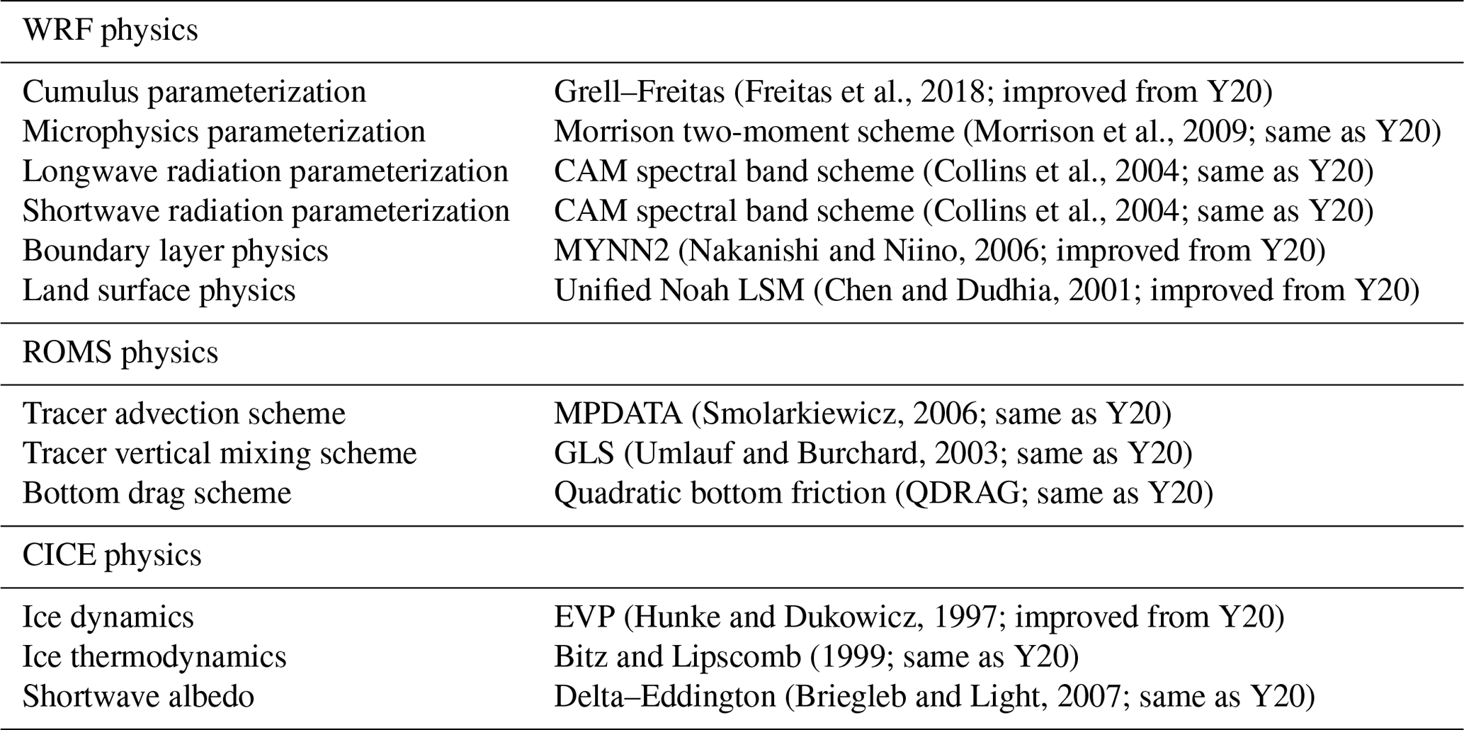
As described in Y20, CAPS has been developed by coupling the Community Ice CodE (CICE) with the Weather Research and Forecasting Model (WRF) and the Regional Ocean Modeling System (ROMS) based on the framework of the Coupled Ocean-Atmosphere-Wave-Sediment Transport (COAWST) (Warner et al., 2010). The general description of each model component in CAPS is referred to Y20. The advantage of CAPS is its model components have a variety of physics for us to choose and capability to integrate follow-up improvements of physical parameterizations. With recent achievements of community efforts, we update CAPS based on newly released WRF, ROMS, and CICE models. During this update, we focus on the Rapid Refresh (RAP) physics in the WRF model, the oceanic tracer advection scheme in the ROMS model, and sea ice thermodynamics in the CICE model (see details in Sect. 3), and investigate physical processes linking them to Arctic sea ice simulation and prediction. The same physical parameterizations described in Y20 are used here for the control simulation (see Table 1). Major changes in physical parameterizations as well as the model infrastructure in the WRF, ROMS, and CICE models are described in Sect. 3.

Table 1 The summary of physic parameterizations used in the Y21_CRTL experiment.

As described in Y20, the Parallel Data Assimilation Framework (PDAF, Nerger and Hiller, 2013) was implemented in CAPS, which provides a variety of optimized ensemble-based Kalman filters. The local error subspace transform Kalman filter (LESTKF; Nerger et al., 2012) is used to assimilate satellite-observed sea ice parameters. The LESTKF projects the ensemble onto the error subspace and then directly computes the ensemble transformation in the error subspace. This results in better assimilation performance and higher computational efficiency compared to the other filters as discussed in Nerger et al. (2012).

The initial ensembles are generated by applying the second-order exact sampling (Pham, 2001) to simulated sea ice state vectors (ice concentration and thickness) from a 1-month free run, and then assimilating sea ice observations, including (1) the near-real-time daily Arctic sea ice concentration processed by the National Aeronautics and Space Administration (NASA) team algorithm (Maslanik and Stroeve, 1999) obtained from the National Snow and Ice Data Center (NSIDC) (https://nsidc.org/data/NSIDC-0081/, last access: 27 June 2021) and (2) a combined monthly sea ice thickness derived from the CryoSat-2 (Laxon et al., 2013; obtained from http://data.seaiceportal.de, last access: 27 June 2021), and daily sea ice thickness derived from the Soil Moisture and Ocean Salinity (SMOS; Kaleschke et al., 2012; Tian-Kunze et al., 2014; obtained from https://icdc.cen.uni-hamburg.de/en/l3c-smos-sit.html, last access: 27 June 2021). To address the issue that sea ice thicknesses derived from CryoSat-2 and SMOS are unavailable during the melting season, the melting season ice thickness is estimated based on the seasonal cycle of the Pan-Arctic Ice Ocean Modeling and Assimilation System (PIOMAS) daily sea ice thickness (Zhang and Rothrock, 2003).

Different from Y20, in this study, we change the localization radius from two to six grids during the assimilation procedures to reduce some instability during initial Arctic sea ice simulations associated with two localization radii. As shown in Fig. S1 in the Supplement, the ice thickness with two localization radii and 1.5 m uncertainty (used in Y20) shows some discontinuous features (Fig. S1a), which tend to result in numerical instability during the initial integration. Such discontinuous features are obviously corrected with six localization radii and 0.75 m uncertainty (Fig. S1b). Following Y20, here we test the 2018 prediction experiment with six localization radii for the data assimilation, which shows very similar temporal evolution of the total Arctic sea ice extent for the July experiment relative to that of Y20, although it (red solid line) predicts slightly less ice extent than that of Y20 (blue line) (Supplement Fig. S2). In this study, this configuration is designated as the reference for the following assessment of the updated CAPS (hereafter Y20_MOD).

For the evaluation of Arctic sea ice prediction, the Sea Ice Index (Fetterer et al., 2017; obtained from https://nsidc.org/data/G02135, last access: 27 June 2021) is used as the observed total sea ice extent, and the NSIDC sea ice concentration (SIC) derived from Special Sensor Microwave Imager/Sounder (SSMIS) with the NASA team algorithm (Cavalieri et al., 1996; obtained from https://nsidc.org/data/nsidc-0051, last access: 27 June 2021) is also used. For the assessment of the simulated atmospheric and oceanic variables, the European Centre for Medium-Range Weather Forecasts (ECMWF) reanalysis version 5 (ERA5; Hersbach et al., 2020; obtained from https://cds.climate.copernicus.eu, last access: 27 June 2021) and National Oceanic and Atmospheric Administration (NOAA) Optimum Interpolation (OI) Sea Surface Temperature (SST) (Reynolds et al., 2007; obtained from https://psl.noaa.gov/data/gridded/data.noaa.oisst.v2.highres.html, last access: 27 June 2021) are utilized. For the comparison of spatial distribution, SIC, ERA5, and OISST are interpolated to the model grid.

3 Evaluation of updated CAPS

3.1 Experiment designs and methodology

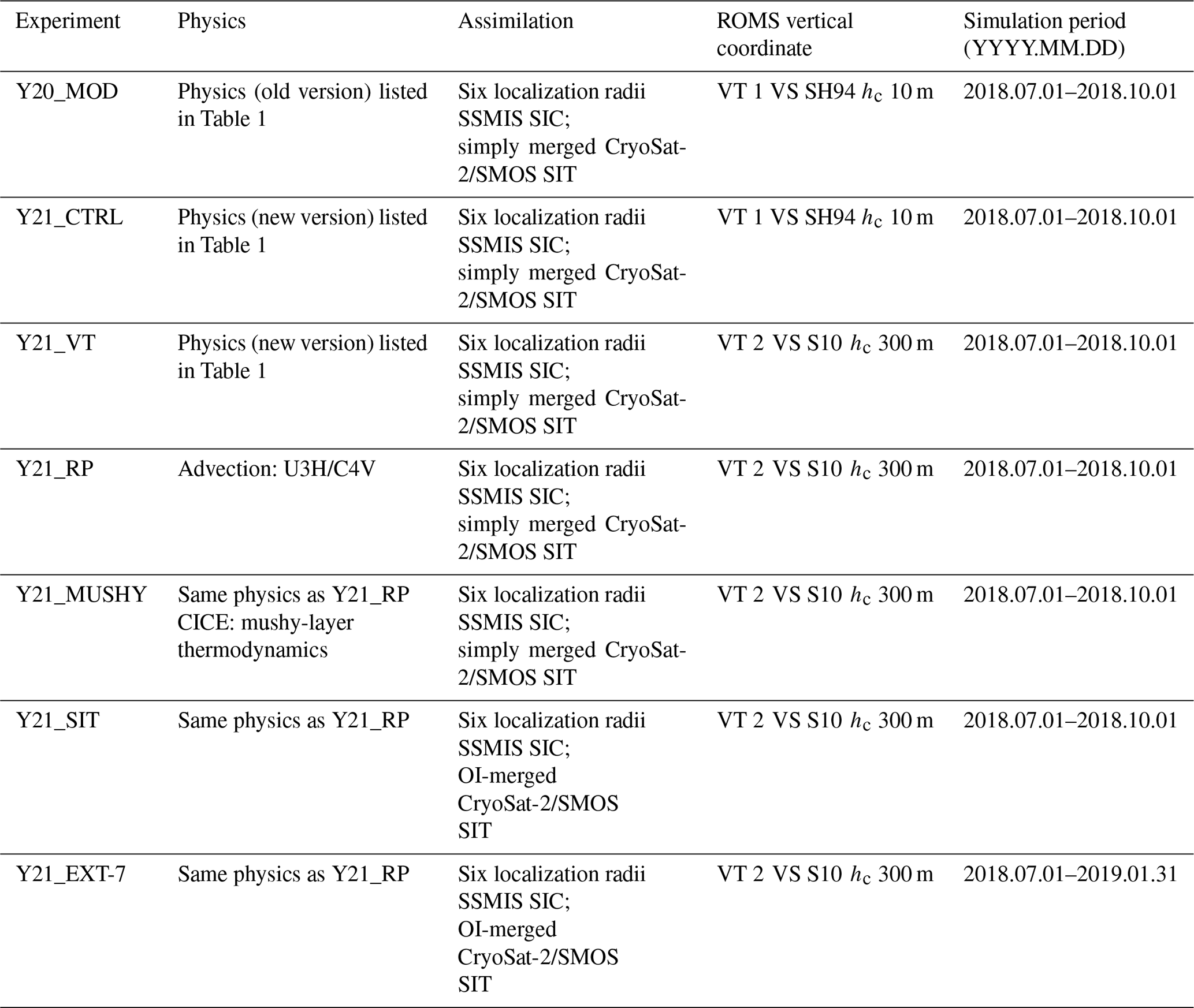
The model domain includes 319 (449) x (y) grid points with a ∼ 24 km grid spacing for all model components (see Fig. 2 in Y20). The WRF model uses 50 vertical levels, the ROMS model uses 40 vertical levels, and the CICE model uses 7 ice layers, 1 snow layer, and 5 categories of sea ice thickness. The coupling frequency across all model components is 30 min. Initial and boundary conditions for the WRF and ROMS models are generated from the Climate Forecast System version 2 (CFSv2, Saha et al., 2014) operational forecast archived at NCEP (http://nomads.ncep.noaa.gov/pub/data/nccf/com/cfs/prod/, last access: 27 June 2021). Sea ice initial conditions are generated from the data assimilation described in Sect. 2. Ensemble predictions with eight members are conducted. A set of numerical experiments for the Pan-Arctic seasonal sea ice prediction with different physics, starting from 1 July to 1 October for the year of 2018, has been conducted. Table 2 provides the details of these experiments that allow us to examine physical processes linking improved and changed physical parameterizations in the updated CAPS to Arctic sea ice simulation and prediction.

Table 2 The summary of the prediction experiments and details of experiment designs. Note that all experiments use the CFS operational forecasts as initial and boundary conditions. VT: vertical transformation function; VS: vertical stretching function; SH94: stretching function of Song and Haidvogel (1994); S10: stretching function of Shchepetkin (2010).

In this study, sea ice extent is calculated as the sum of area of all grid cells with ice concentration greater than 15 %. Besides the total Arctic sea ice extent, we also calculate the ice extent for the following subregions: (1) Beaufort and Chukchi seas (60–80^∘ N, 120–180^∘ W), (2) East Siberian and Laptev seas (60–80^∘ N, 180–90^∘ E), and (3) Barents, Kara, and Greenland seas (60–80^∘ N, 90^∘ E–30^∘ W). To further assess the predictive skill of Arctic sea ice predictions, we show the climatology prediction (CLIM, the period of 1998–2017) and the damped anomaly persistence prediction (DAMP). Following Van den Dool (2006), the DAMP prediction is generated from the initial sea ice extent anomaly (relative to the 1998–2017 climatology) scaled by the autocorrelation and the ratio of standard deviation between different lead times and initial times (see the DAMP equation in Y20).

In order to understand physical contributors that drive the evolution of Arctic sea ice state (the standard variables of the ice concentration and thickness), the mass budget of Arctic sea ice for all experiments is analyzed in this study as defined in Notz et al. (2016, Appendix E), including

• sea ice growth in supercooled open water (frazil),

• sea ice growth at the bottom of the ice (basal growth),

• sea ice growth due to transformation of snow to sea ice (snowice),

• sea ice melt at the air–ice interface (top melt),

• sea ice melt at the bottom of the ice (basal melt),

• sea ice melt at the sides of the ice (lateral melt), and

• sea ice mass change due to dynamics-related processes (e.g., advection) (dynamics).

These diagnostic variables are determined by saving the ice mass tendency of above processes separately every time step and integrated to output the daily mean value.

3.2 Impacts of the RAP physics in the WRF model

To examine the performance of the upgrades of physical parameterization in component models in CAPS one step at a time compared to its predecessor in Y20, we define the Y21_CTRL experiment that uses the RAP physics in the WRF model (see Table 2 for differences between Y21_CTRL and Y20_MOD). Recently, the Rapid Refresh (RAP) model, a high-frequency weather prediction/assimilation modeling system operational at the National Centers for Environmental Prediction (NCEP), has made some improvements in the WRF model physics (Benjamin et al., 2016), including improved Grell–Freitas convection scheme (GF) and Mellor–Yamada–Nakanishi–Niino planetary boundary layer scheme (MYNN). For the GF scheme, the major improvements relative to the original scheme (Grell and Freitas, 2014) include (1) a beta probability density function used as the normalized mass flux profile for representing height-dependent entrainment/detrainment rates within statistical-averaged deep convective plumes, which is given as

$$Z_{\mathrm{u},\mathrm{d}}\left(r_k\right)=c{r}_k^{\mathit{\alpha }}-{\left(\mathrm{1}-r_k\right)}^{\mathit{\beta }}-\mathrm{1},$$

where Z_u,d is the mass flux profiles for updrafts and downdrafts, c is a normalization constant, r_k is the location of the mass flux maximum, and α and β determine the skewness of the beta probability density function, and (2) the ECMWF approach used for momentum transport due to convection (Biswas et al., 2020; Freitas et al., 2018, 2021). For the MYNN scheme, the RAP model improves the mixing-length formulation, which is designed as

$${\displaystyle \frac{\mathrm{1}}{l_{\mathrm{m}}}}={\displaystyle \frac{\mathrm{1}}{l_{\mathrm{s}}}}+{\displaystyle \frac{\mathrm{1}}{l_{\mathrm{t}}}}+{\displaystyle \frac{\mathrm{1}}{l_{\mathrm{b}}}},$$

where l_m is the mixing length, l_s is the surface length, l_t is the turbulent length, and l_b is the buoyancy length. Compared to the original scheme, the RAP model changed coefficients in the formulation of l_s, l_t, and l_b for reducing the near-surface turbulent mixing and the diffusivity of the scheme. The RAP model also removes numerical deficiencies to better represent subgrid-scale cloudiness (Benjamin et al., 2016; see Appendix B) compared to the original scheme (Nakanishi and Nino, 2009). In addition, some minor issues in the Noah land surface model (LSM) (Chen and Dudhia, 2001) have been fixed, including discontinuous behavior for soil ice melting, negative moisture fluxes over glacial areas, and those associated with snow melting.

Apparently, the above RAP physics can have influence on the behavior of simulated atmospheric thermodynamics (i.e., radiation, temperature). Figures 1 and 2 show the spatial distribution of the ERA5 surface downward solar and thermal radiation (SWDN and LWDN), the prediction errors (ensemble mean minus ERA5) of Y20_MOD, and the difference between Y21_CTRL and Y20_MOD. For July, Y20_MOD (Fig. 1d) results in less SWDN over most of the ocean basins, as well as Alaska and the northeast US, western Siberia, and eastern Europe, but more SWDN over southern and eastern Siberia compared with ERA5. For August and September (Fig. 1e–f), the spatial distribution is generally similar to that of July, except in eastern Siberia (less SWDN) and northern Canada (more SWDN) in August. It appears that the magnitude of the prediction errors tends to decrease over the areas with large prediction errors as the prediction time increases (i.e., July vs. September). Compared with Y20_MOD, the RAP physics in Y21_CTRL results in large areas with smaller prediction errors in July (e.g., the positive difference between Y21_CTRL and Y20_MOD reduces the negative prediction errors in Y20_MOD), except in the north Pacific (especially the Sea of Okhotsk) and north Canada (Fig. 1g). For August and September (Fig. 1h, i), encouragingly, there are more areas with smaller prediction errors.

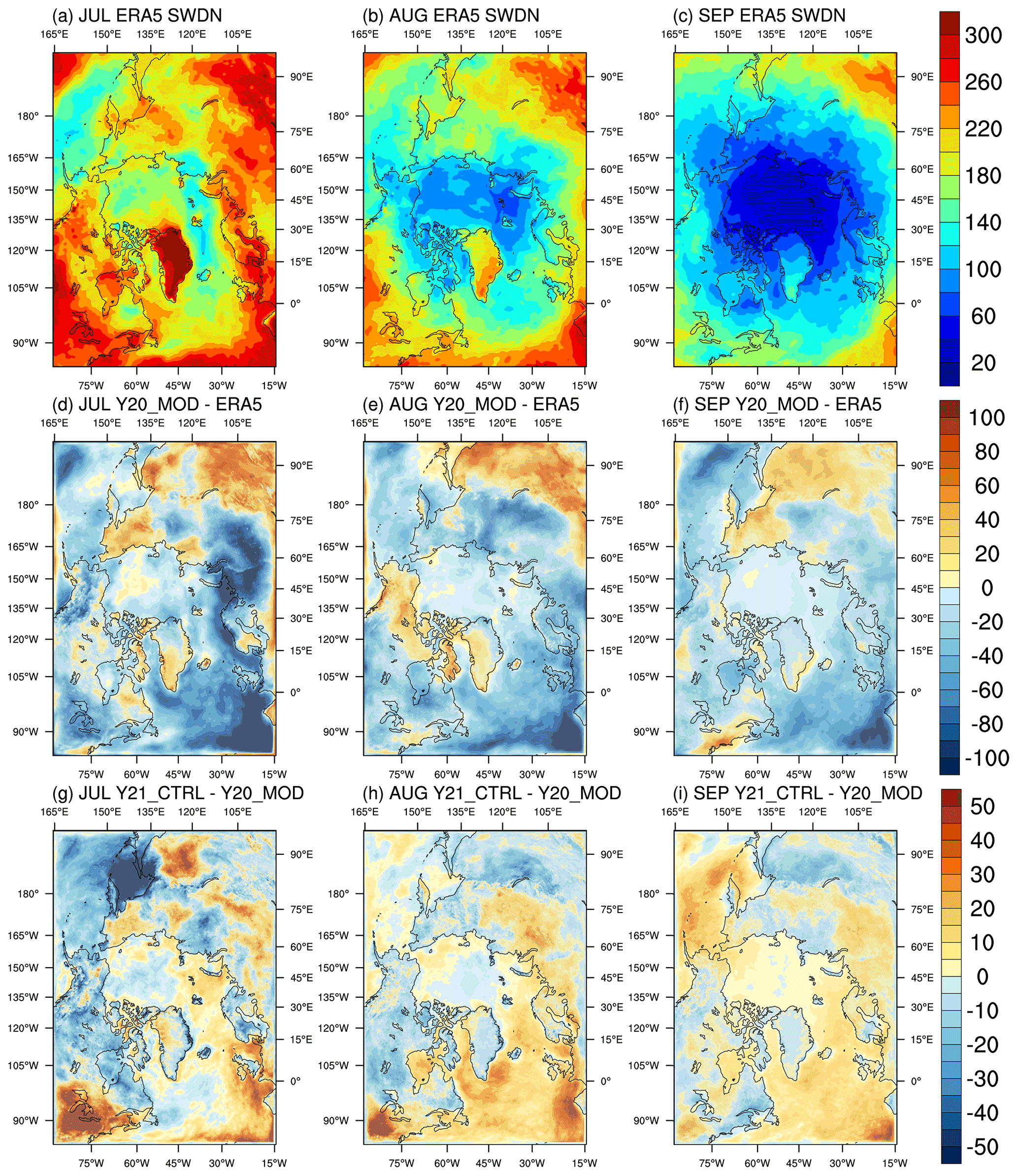
Figure 1 ERA5 monthly mean of downward shortwave radiation at the surface for (a) July, (b) August, and (c) September, the difference between Y20_MOD and ERA5 for (d) July, (e) August, and (f) September, and the difference between Y21_CTRL (changes in the atmospheric physics) and Y20_MOD (the original CAPS) for (g) July, (h) August, and (i) September.

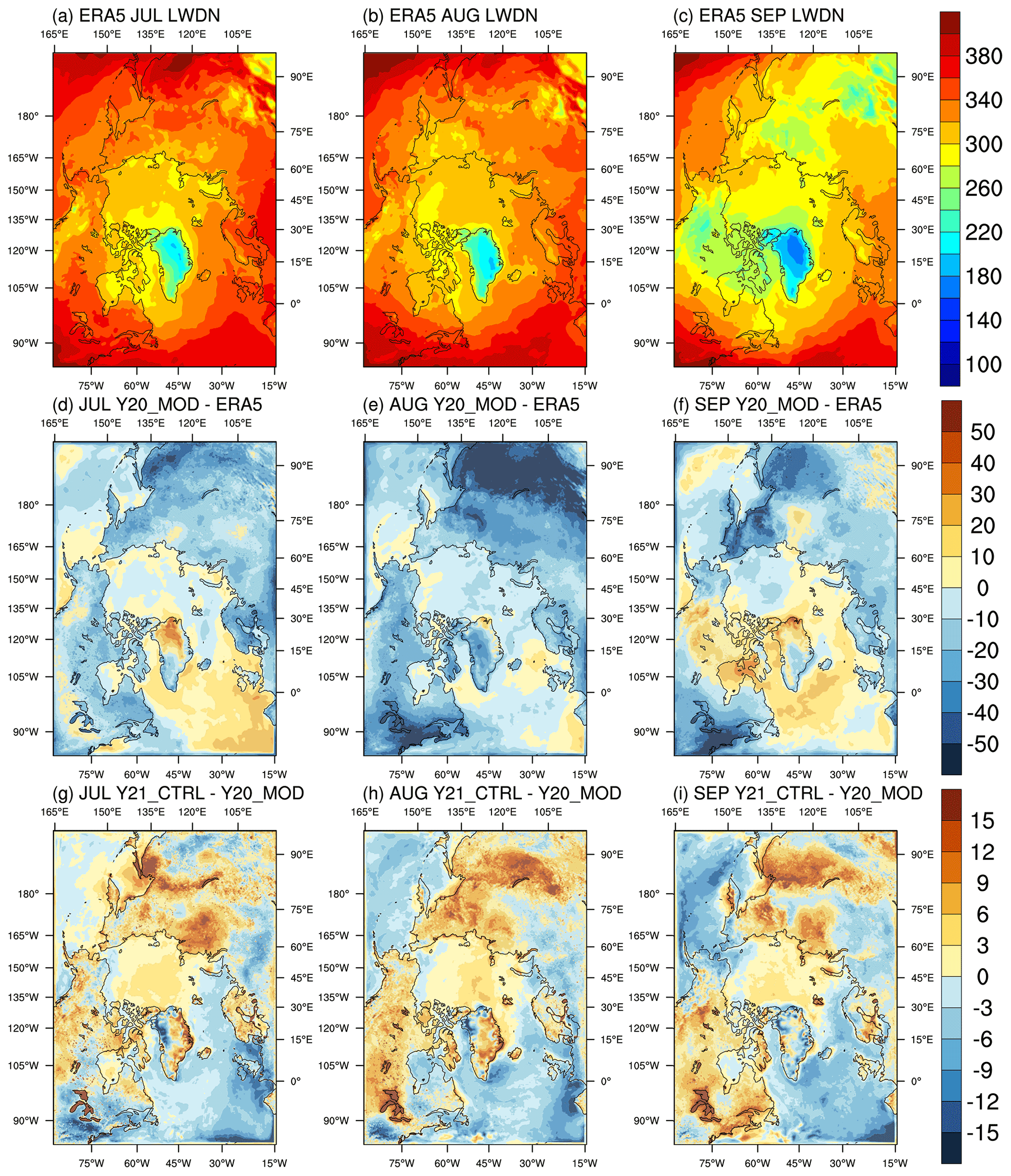
Figure 2 Same as Fig. 1 but for downward thermal radiation at the surface.

In contrast to SWDN, the prediction errors of LWDN in Y20_MOD have a much smaller magnitude (up to 100 W m⁻² in SWDN vs. 50 W m⁻² in LWDN) for the entire prediction period (Fig. 2d–f). For July, Y20_MOD (Fig. 2d) simulates less LWDN over most of the model domain compared with ERA5, except the Atlantic sector and north Greenland. For August, the areas with negative prediction errors expand and the magnitude of prediction errors increases (particularly in southeastern Siberia and the northeast US) compared to that of July (Fig. 2e). For September (Fig. 2f), the spatial distribution of LWDN is mostly similar to that of July, except that north Canada and Canadian Archipelago show positive prediction errors. The Y21_CTRL experiment with the RAP physics tends to reduce the prediction errors in Y20_MOD, especially over eastern Siberia and the Atlantic sector in July to September (Fig. 2g–i). However, Y21_CTRL results in larger bias in the central northern Atlantic in August than that of Y20_MOD (Fig. 2h).

Figure 3 shows the spatial distribution of the ERA5 2 m air temperature, the prediction errors of Y20_MOD, and the difference between Y21_CTRL and Y20_MOD. For Y20_MOD, the predicted air temperature in July has small cold prediction errors over all ocean basins, small-to-moderate cold prediction errors (∼ 3–5 ^∘C) over Canada and Siberia, and moderate-to-large cold prediction errors (∼ 6–9 ^∘C) over eastern Europe (Fig. 3d). In August (Fig. 3e), the cold prediction errors over most of the model domain are increased; in particular, a very large cold prediction error (over 10 ^∘C) is located over east Siberia. In September, these cold prediction errors are decreased relatively, and some warm prediction errors are found in the north of Greenland (Fig. 3f). With the adaptation of the RAP physics in the WRF model, Y21_CTRL, in general, produces a warmer state in most of the model domain compared to that of Y20_MOD during the entire prediction period. For July (Fig. 3g), the predicted air temperature is slightly warmer over the Arctic Ocean, the Pacific, and Atlantic sectors, moderately warmer (∼ 1–2 ^∘C) over central and eastern Siberia and the Canadian Archipelago but the slightly colder over northern Canada than that of Y20_MOD. For August and September (Fig. 3h), most of the model domain is warmer in Y21_CTRL than that of Y20_MOD, in particular excessive cold prediction errors shown in Y20_MOD over Siberia are reduced notably (∼ 2.5–4 ^∘C). We notice that the RAP physics does not have significant impacts on atmospheric circulations, given that Y21_CTRL and Y20_MOD have very similar wind patterns (not shown).

Figure 3 Same as Fig. 1 but for near-surface air temperature.

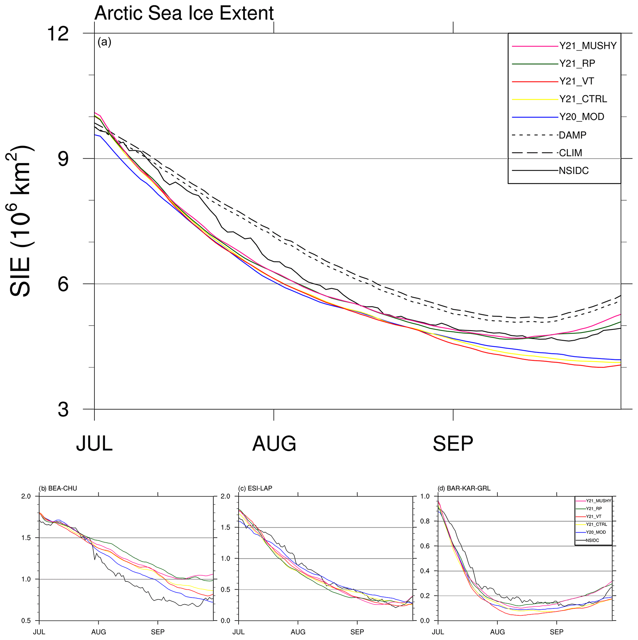
Figure 4 (a) Time series of Arctic sea ice extent for the observations (black line) and the ensemble mean of Y20_MOD (blue line, the original CAPS), Y21_CTRL (yellow line, changes in the atmospheric physics), Y21_VT (red line, changes in the ocean vertical coordinate), Y21_RP (green line, changes in the oceanic advection), and Y21_MUSHY (pink line, changes in sea ice thermodynamics). Dashed and dotted lines are the climatology and the damped anomaly persistence predictions. Bottom panel: time series of the observed (black line) and the ensemble mean of regional sea ice extents for Y20_MOD (blue line), Y21_CTRL (yellow line), Y21_VT (red line), Y21_RP (green line), and Y21_MUSHY (pink line) for the (a) Beaufort–Chukchi seas, (b) East Siberian–Laptev seas, and (c) Barents–Kara–Greenland seas.

Figure 4 shows the temporal evolution of the ensemble mean of the predicted Arctic sea ice extent along with the NSIDC observations. In terms of total ice extent, compared to the Y20_MOD experiment (blue line), the Y21_CTRL experiment (yellow line) produces ∼ 0.5 million km² more ice extent at the initial. Note that the difference in the initial ice extent is related to that sea ice fields in Y20_MOD and Y21_CTRL (as well as other experiments listed in Table 2) are initialized based on 1-month free runs (Sect. 2), which use different physical configurations listed in Table 2. These 1-month free runs do not have the same evolution in sea ice fields and result in different initial ice fields after data assimilation. The ice extent in Y21_CTRL decreases faster than Y20_MOD during the first 2-week integration. After that, they track each other closely and predict nearly the same minimum ice extent (∼ 4.3 million km²). Like Y20_MOD, Y21_CTRL still has a delayed ice recovery in late September compared to the observations. Compared with the CLIM and DAMP predictions (dashed and dotted black lines), both Y20_MOD and Y21_CTRL have smaller prediction errors in August but comparable prediction errors after early September.

The difference in sea ice extent becomes larger at regional scales; in the East Siberian–Laptev seas, Y21_CTRL shows faster ice decline after mid-July than that of Y20_MOD, whereas in the Beaufort–Chukchi seas, Y21_CTRL predicts slower ice retreat after late July than that of Y20_MOD (Fig. 4a, b). They are consistent with Y21_CTRL predicting warmer (relatively colder) temperature than that of Y20_MOD in the East Siberian–Laptev (Beaufort–Chukchi) seas. Both Y20_MOD and Y21_CTRL agree well with the observations in the Barents–Kara–Greenland seas (Fig. 4c). Compared with the observations, Y20_MOD performs relatively better in regional ice extent than Y21_CTRL. Figure 5 shows the spatial distribution of the NSIDC sea ice concentration and the difference between the predicted ice concentration and the observations for all grid cells such that the predictions and the observations both have at least 15 % ice concentration. The vertical and horizontal lining areas represent the difference of the ice edge location. Like regional ice extent shown in Fig. 4, Y21_CTRL predicts lower (higher) ice concentration along the East Siberian–Laptev (Beaufort–Chukchi) seas (Fig. 5e₁–e₃). Y21_CTRL also predicts less ice in the central Arctic Ocean in August and September, which is consistent with warmer temperature in Y21_CTRL relative to Y20_MOD.

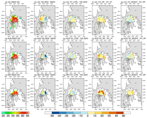
Figure 5 Monthly mean of sea ice concentration for (a) July, (b) August, and (c) September of the NSIDC observations, and the difference between the all prediction experiments and the observations for (d₁–g₁) July, (d₂–g₂) August, and (d₃–g₃) September. Vertical- and horizontal-line areas represent the difference of ice edge location (15 % concentration).

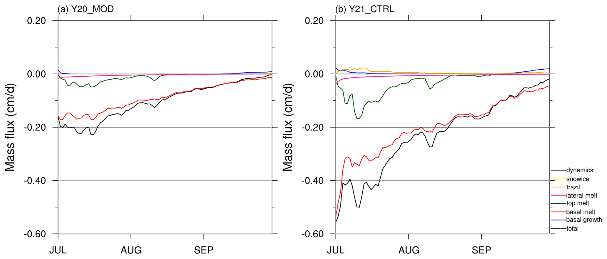
Figure 6 Time series of sea ice mass budget terms for (a) Y20_MOD (the original CAPS) and (b) Y21_CTRL (changes in the atmospheric physics).

Figure 6 shows the evolution of sea ice mass budget terms of Y20_MOD and Y21_CTRL, averaged with cell-area weighting over the entire model domain. During the entire prediction period, most of the ice loss in Y20_MOD and Y21_CTRL is caused by basal melting. The surface melting has a relatively small contribution in the total ice loss and mainly occurs in July. However, compared with Y20_MOD (Fig. 6a), Y21_CTRL (Fig. 6b) shows much larger magnitude for basal and surface melt. In a fully coupled predictive model, the changes of sea ice are determined by the fluxes from the atmosphere above and the ocean below. Associated with the increased downward radiation of the above RAP physics, Y21_CTRL absorbs more shortwave radiation (SWABS, Fig. 7a) and allows more penetrating solar radiation into the upper ocean below sea ice (SWTHRU, Fig. 7b) than that of Y20_MOD, especially in July. This explains why Y21_CTRL has larger magnitude of surface and basal melting terms. Although Y21_CTRL show larger magnitude in surface and basal melting than that of Y20_MOD, the ice extent in Y21_CTRL and Y20_MOD shown in Fig. 4 shows a similar evolution. The effect of larger surface and basal melting in Y21_CTRL is largely reflected in the ice thickness change. As shown in Fig. S3, Y21_CTRL has thinner ice thickness than that of Y20_MOD, in the East Siberian–Laptev seas in July and in much of central Arctic Ocean in August and September.

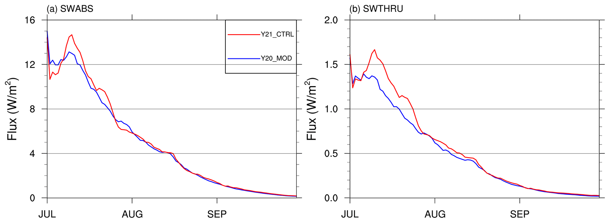
Figure 7 Time series of (a) shortwave radiation absorbed by ice surface and (b) penetrating shortwave radiation to the upper ocean averaged over ice-covered grid cells for Y20_MOD (blue line, the original CAPS) and Y21_CTRL (red line, changes in the atmospheric physics).

3.3 Impacts of the tracer advection in ROMS model

Currently, the ROMS model that uses a generalized topography-following coordinate has two vertical coordinate transformation options:

$$\begin{array}{}\text{(1)}& {\displaystyle }& {\displaystyle }\begin{array}{c}z\left(x,y,\mathit{\sigma },t\right)=S\left(x,y,\mathit{\sigma }\right)+\mathit{\zeta }\left(x,y,t\right)\left[\mathrm{1}+\frac{S\left(x,y,\mathit{\sigma }\right)}{h\left(x,y\right)}\right]\\ S\left(x,y,\mathit{\sigma }\right)=h_{\mathrm{c}}\mathit{\sigma }+\left[h\left(x,y\right)-h_{\mathrm{c}}\right]C\left(\mathit{\sigma }\right)\end{array}\mathrm{\text{or}}\text{(2)}& {\displaystyle }& {\displaystyle }\begin{array}{c}z\left(x,y,\mathit{\sigma },t\right)=\mathit{\zeta }\left(x,y,t\right)+\left[\mathit{\zeta }\left(x,y,t\right)+h\left(x,y\right)\right]S\left(x,y,\mathit{\sigma }\right)\\ S\left(x,y,\mathit{\sigma }\right)=\frac{h_{\mathrm{c}}\mathit{\sigma }+h\left(x,y\right)C\left(\mathit{\sigma }\right)}{h_{\mathrm{c}}+h\left(x,y\right)},\end{array}\end{array}$$

where $S\left(x,y,\mathit{\sigma }\right)$ is a nonlinear vertical transformation function, $\mathit{\zeta }\left(x,y,t\right)$ is the free surface, h(x,y) is the unperturbed water column thickness, C(σ) is the non-dimensional, monotonic vertical stretching function, and h_c controls the behavior of the vertical stretching. In Y20, we used the transformation (1) and the vertical stretching function introduced by Song and Haidvogel (1994). However, the vertical transformation (1) has an inherent limitation for the value of h_c (expected to be the thermocline depth), which must be less than or equal to the minimum value in h(x,y). As a result, h_c was chosen as 10 m due to the limitation of the minimum value in  h(x,y) in Y20. This limitation is removed with the vertical transformation (2) and h_c can be any positive value. Here, the Y21_VT experiment is conducted to examine the impact of the vertical transformation in the ROMS model on seasonal Arctic sea ice simulation and prediction, which uses the vertical transformation (2), the Shchepetkin vertical stretching function (a function introduced in a research version of ROMS at University of California, Los Angeles), and 300 m for h_c. As shown in Supplement Figs. S4–S5, compared to Y21_CTRL, Y21_VT is less sensitive to the bathymetry and its layers are more evenly distributed in the upper 300 m. With the changes of vertical layers of the upper ocean, the Y21_VT experiment has minor SST changes relative to Y21_CTRL. The simulated temporal evolution of total ice extent of Y21_VT (Fig. 4, red line) resembles that of Y21_CTRL (Fig. 4, yellow line), although some differences are seen at the regional scale in the areas with shallow water (e.g., East Siberian, Laptev, Barents, and Kara seas). The configuration of Y21_VT is used in the following experiments.

It has been recognized that the tracer advection and the vertical mixing schemes have important effects on ocean and sea ice simulation (e.g., Liang and Losch, 2018; Naughten et al., 2017). Here, the Y21_RP experiment is designated to explore the influence of different advection schemes in the ROMS model. Specifically, the tracer advection scheme is changed from the multidimensional positive definite advection transport algorithm (MPDATA; Smolarkiewicz, 2006) to the third-order upwind horizontal advection (U3H; Rasch, 1994; Shchepetkin and McWilliams, 2005) and the fourth-order centered vertical advection schemes (C4V; Shchepetkin and McWilliams, 1998, 2005). The MPDATA scheme applied in Y20_MOD, Y21_CTRL, and Y21_VT is a non-oscillatory scheme but a sign-preserving scheme (Smolarkiewicz, 2006). This means MPDATA is not suitable for tracer fields having both positive and negative values (i.e., temperature with degrees Celsius in the ROMS model). The upwind third-order (U3H) scheme used in Y21_RP is an oscillatory scheme but it significantly reduces oscillations compared to other centered schemes (e.g., Hecht et al., 2000; Naughten et al., 2017) available in the ROMS model.

Figure 8 shows the spatial distribution of the SST changes of Y21_VT and Y21_RP relative to Y21_CTRL (as well as the OISST and the difference between Y21_CTRL and OISST). In general, Y21_CTRL shows cold prediction errors in the North Pacific (∼ 2 ^∘C) and the Atlantic (∼ 3 ^∘C) compared to those of OISST in July, and these cold prediction errors are enhanced as the prediction time increases (to 3–5 ^∘C, Fig. 8d–f). With the U3H and C4V tracer advection schemes in Y21_RP, cold prediction errors shown in Y21_CTRL are reduced significantly in the North Pacific and Atlantic, but SST under sea ice in much of the Arctic Ocean is slightly colder than that of Y21_CTRL (Fig. 8j–l).

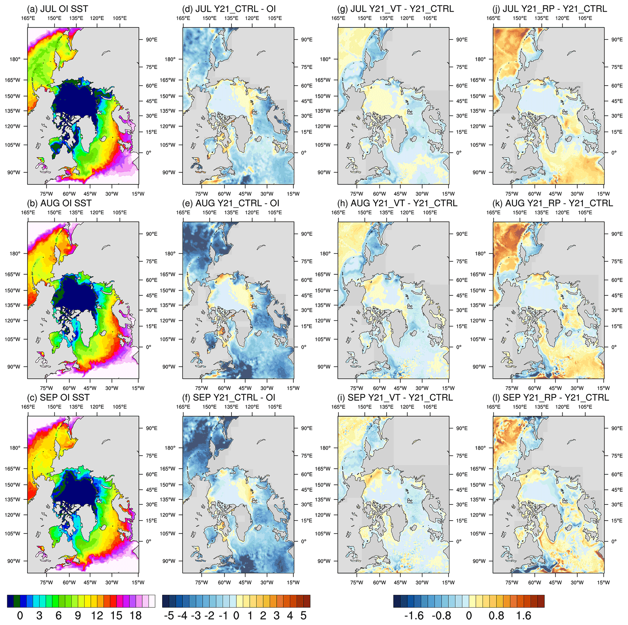
Figure 8 First column: monthly mean of sea surface temperature for (a) July, (b) August, and (c) September of the OI SST. Second column: the difference between Y21_CTRL and the OI SST for (d) July, (e) August, and (f) September. Right panel: monthly mean of sea surface temperature difference between Y21_VT/Y21_RP and Y21_CTRL for (g) July, (h) August, and (i) September of Y21_VT, and (j) July, (k) August, and (l) September of Y21_RP.

Y21_RP (Fig. 4, green line) shows a comparable temporal evolution of the ice extent as Y21_CTRL (as well as Y21_VT) until near the end of July. After that, the ice melting slows down (closer to the observations) and the ice extent begins to recover earlier (after the first week of September) in Y21_RP compared to that of Y21_CRTL. This leads to much smaller prediction error in seasonal minimum ice extent relative to the observation. Y21_RP also shows better predictive skill after late August compared with the CLIM and DAMP predictions (dashed and dotted black lines). This suggests the delayed ice recovery in late September shown in Y20_MOD, Y21_CTRL, and Y21_VT is in part due to the choice of ocean advection and vertical mixing schemes, which change the behavior of ocean state. At the regional scale, the slower ice decline after July and earlier recovery of the ice extent in September mainly occur in the Beaufort–Chukchi and Barents–Kara–Greenland seas compared to that of Y21_CTRL (Fig. 4a, c). With the U3H and C4V schemes, the Y21_RP experiment simulates higher sea ice concentration than that of Y21_VT (Fig. 5f₁–f₃). For September, the Y21_RP experiment better predicts the ice edge location in the Atlantic sector of the Arctic (i.e., smaller areas with horizontal and vertical linings) compared to the experiments described above (not shown).

Figure 9 shows the evolution of sea ice mass budget terms of Y21_VT and Y21_RP. Relative to Y21_VT, Y21_RP (with U3H and C4V schemes) results in increased frazil ice formation in July, which is partly compensated by increased surface melting. Y21_RP also leads to increased basal growth in mid- and late September (Fig. 9a, b).

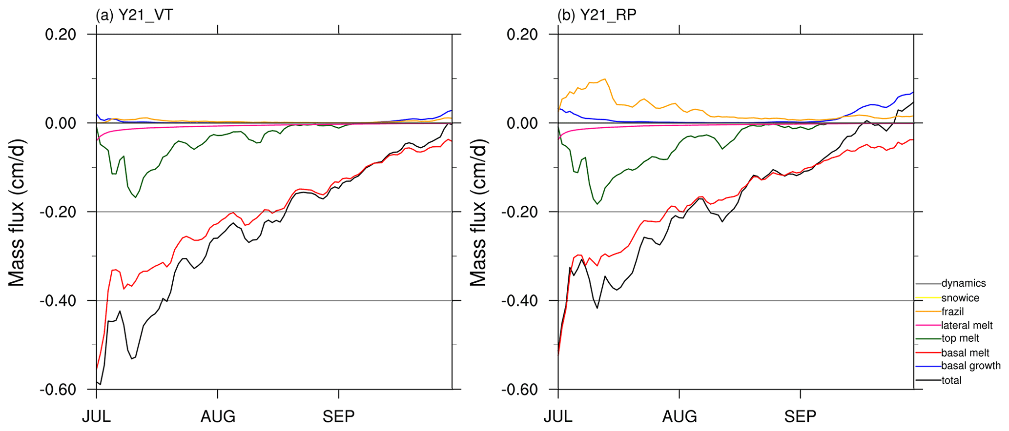
Figure 9 Same as Fig. 6 but for (a) Y21_VT (changes in the ocean vertical coordinate) and (b) Y21_RP (changes in the oceanic advection).

Figure 10 (a) The average temperature profile of upper 150 m under ice-covered areas for the difference between Y21_RP and Y21_VT. Panel (b) is the same as (a) but for the salinity profile.

Figure 10 shows the difference in the vertical profile of ocean temperature and salinity in the upper 150 m averaged for the central Arctic Ocean between Y21_RP and Y21_VT. The ocean temperature in the surface layer of Y21_RP is slightly colder during the prediction period compared to that of Y21_VT (Fig. 10a), especially in August and September. Moreover, the water in the surface layer (0–20 m) of Y21_RP is fresher than that of Y21_VT (Fig. 10b). It reduces the freezing temperature and favors frazil ice formation. In CAPS, frazil ice formation is determined by the freezing potential, which is the vertical integral of the difference between temperature in upper ocean layer and the freezing temperature in the upper 5 m layer. The temperature of supercooled water is adjusted based on the freezing potential to form new ice and rejects brine into the ocean that leads to saltier water between 20–50 m in Fig. 10. It should be noted that the increased frazil ice formation in July in Y21_RP might also be the result of model adjustment and/or numerical error. The oscillatory behavior of U3H scheme can make the temperature fall below the freezing point and then instantaneously form new ice (as well as temperature and salinity adjustments).

3.4 Impacts of sea ice thermodynamics in the CICE model

In Y20, we used sea ice thermodynamics introduced by Bitz and Lipscomb (1999; hereafter BL99) as the setup of CAPS, which assumes a fixed vertical salinity profile based on observations. The new CICE model includes a mushy-layer ice thermodynamics introduced by Turner et al. (2013), which simulates vertically and time-varying prognostic salinity and associated effects on thermodynamic properties of sea ice. In the Y21_MUSHY experiment, we change the ice thermodynamics from BL99 to MUSHY (Table 2) to examine whether improved ice thermodynamics has noticeable influence on Arctic sea ice simulation and prediction at seasonal timescale. Compared to Y21_RP, Y21_MUSHY (Fig. 4, pink line) produces a very similar evolution of total ice extent. However, it simulates relatively larger ice extent near the end of September, which is also reflected by the basin-wide increased ice cover shown in Fig. 5h₃. At the regional scale, compared to Y21_RP, Y21_MUSHY predicts less ice in August in the Beaufort–Chukchi seas. The opposite is the case for the East Siberian–Laptev seas (Fig. 4a, b).

Figure 11 shows the difference of the ensemble mean of the predicted ice thickness between Y21_MUSHY and Y21_RP. Compared with Y21_RP, Y21_MUSHY simulates thicker ice (from ∼ 0.2 m in July to over 0.4 m in September) extending from the Canadian Arctic, through the central Arctic Ocean, to the Laptev Sea (Fig. 11a–c). This seems to be consistent with previous studies, which show that the mushy-layer thermodynamics simulates thicker ice than BL99 thermodynamics in both standalone CICE (Turner and Hunke, 2015) and the fully coupled (Bailey et al., 2020), but Y21_MUSHY shows thinner ice (∼ 0.2 m) in an arc extending from the north of Alaska to the north of eastern Siberia compared to Bailey et al. (2020). Note that Y21_MUSHY focuses the effects of mushy thermodynamics on a seasonal timescale, while the results in Bailey et al. (2020) are based on 50-year simulations.

Figure 11 Monthly mean of sea ice thickness difference between Y21_MUSHY (changes in sea ice thermodynamics) and Y21_RP for (a) July, (b) August, and (c) September.

Compared to Y21_RP, the mass budget of Y21_MUSHY (Fig. S6) shows that both surface melting and frazil ice formation terms are increased. This compensation between surface melting and frazil ice formation from the mushy-layer thermodynamics in CAPS leads to relatively unchanged total ice extent between Y21_MUSHY and Y21_RP (Fig. 4 green and pink lines).

4 Prediction skill of CAPS at longer timescales

The design of Arctic sea ice prediction experiments described above follow the protocol of SIPN, in which the outlook start from 1 June, 1 July, and 1 August to predict seasonal minimum of the ice extent in September. It is not clear that how predictive skills of dynamical models participating in SIPN may change for longer periods. Here, we conduct two more experiments to investigate the predictive capability of CAPS beyond the SIPN prediction period. For the prediction experiments discussed above, we use a simple approach to merge CryoSat-2 and SMOS ice thickness by replacing ice thickness less than 1 m in CryoSat-2 data with SMOS data for ice thickness assimilation. Ricker et al. (2017) presented a new ice thickness product (CS2SMOS) based on the optimal interpolation to statistically merge CryoSat-2 and SMOS data. Here, we utilize the configuration of Y21_RP but use CS2SMOS SIT for the assimilation (Y21_SIT; Table 2). The predicted total ice extent is almost identical to Y21_RP in July but has a slightly larger total extent after July than that of Y21_RP (not shown). The configuration of Y21_SIT is used in the following experiments. Taking advantage of the entire prediction period provided by CFS forecasts (7 months), the Y21_EXT-7 experiment is designed to extend the prediction period to the end of January next year (Table 2). Figure 12 shows the temporal evolution of the ensemble mean of the predicted total Arctic sea ice extent (as well as regional ice extent) for Y21_EXT-7. Total ice extent of Y21_EXT-7 exhibits reasonable evolution in terms of seasonal minimum and timing of recovery compared with the observations until late November. Y21_EXT-7 also performs better than that of the CLIM and DAMP predictions (dashed and dotted black lines) until mid-to-late November. After that, Y21_EXT-7 overestimates total ice extent relative to the observations, and such overestimation is largely contributed by more extensive sea ice in the Barents–Kara–Greenland seas (Fig. 12c), which is a result of a sharp increase in the basal growth term after mid-to-late November (not shown).

Figure 12 Same as Fig. 4 but for Y21_EXT-7.

5 Conclusions and discussions

This paper presents and evaluates the updated Coupled Arctic Prediction System (CAPS) designated for Arctic sea ice prediction through a case study for the year of 2018. A set of Pan-Arctic prediction experiments with improved and changed physical parameterizations as well as different configurations starting from 1 July to the end of September is performed for 2018 to assess their impacts of the updated CAPS on the predictive skill of Arctic sea ice at seasonal timescales. Specifically, we focus on the Rapid Refresh (RAP) physics in the WRF model, the oceanic tracer advection scheme in the ROMS model, and sea ice thermodynamics in the CICE model, and investigate physical processes linking them to Arctic sea ice simulation and prediction.

The results show that the updated CAPS with improved physical parameterizations can better predict the evolution of total ice extent compared with its predecessor described in Yang et al. (2020), though the predictions exhibit some prediction errors in regional ice extent. The key improvements of WRF, including cumulus, boundary layer, and land surface schemes, result in improved simulations in downward radiative fluxes and near-surface air temperature. These improvements mainly influence the predicted ice thickness instead of total ice extent. The difference in the predicted ice thickness can have potential impacts on the icebreakers planning their routes across the ice-covered regions. The major changes of ROMS, including tracer advection and vertical mixing schemes, reduce the prediction errors in sea surface temperature and change ocean temperature and salinity structure in the surface layer, leading to improved evolution of the predicted total ice extent (particularly correcting the late ice recovery issue in the previous CAPS). The changes of CICE, including improved ice thermodynamics, have noticeable influences on the predicted ice thickness.

We demonstrate that CAPS can remain skillful beyond the designated period of Sea Ice Prediction Network (SIPN), which has a potential value for stakeholders to make decisions regarding the socioeconomic activities in the Arctic. Although CAPS shows extended predictive skill to the freeze-up period, the prediction produces extensive ice through the basal growth near the end of prediction. The excessive basal growth may be partly due to the fact that the bias of the CFS data propagates into the model domain through lateral boundary conditions and its accumulated effect influences Arctic sea ice simulation during the freeze-up period.

Keen et al. (2021) analyzed the Arctic mass budget of 15 models participated in phase 6 of the Coupled Model Intercomparison Project (CMIP6). We notice that, first, the top melting and the basal melting terms in CMIP6 models have comparable contributions in July, while the top melting term only has ∼ 50 % contribution relative to the basal melting term in CAPS. The updated CAPS with the RAP physics improves the performance of shortwave and longwave radiation at the surface (Figs. 1 and 2). The net flux at the ice surface, however, may still be underestimated in the updated CAPS. Besides, the surface property of sea ice (i.e., the amount of melt ponds, bare ice, and snow) is a factor that influences surface albedo and thus the absorbed shortwave radiation (e.g., Nicolaus et al., 2012; Nicolaus and Katlein, 2013). The prediction experiments starting on 1 July in this study do not consider the initialization of melt ponds (i.e., zero melt pond coverage at the initial). However, melt ponds start to develop in early May based on the satellite observations (e.g., Liu et al., 2015, Fig. 1). The initialization of melt pond based on the observations (e.g., Ding et al., 2020) in CAPS is a direction to improve the representation of the ice surface properties. Second, the mass budget analysis by both Keen et al. (2021) and this study show that the contribution of a lateral melting term is relatively small, which might be due to the fact that CMIP6 models and CAPS assume constant floe size (i.e., 300 m in CICE), which is a critical value to determine the strength of lateral melting (e.g., Horvat et al., 2016; Steele, 1992). Recently, several studies have proposed floe size distribution models (e.g., Bateson et al., 2020; Bennetts et al., 2017; Boutin et al., 2020; Horvat and Tziperman, 2015; Roach et al., 2018, 2019; Zhang et al., 2015, 2016). Incorporating a floe size distribution model in CAPS and understanding its impacts on seasonal Arctic sea ice prediction will be a future direction of developing CAPS. Lastly, the prediction experiments with the upwind advection scheme (i.e., Y21_RP, Y21_EXT-7) show spurious large frazil ice formation, particularity in July, which is different from the analysis shown in Keen et al. (2021). An approach for reducing spurious frazil ice formation is proposed by Naughten et al. (2017), who implemented an upwind flux limiter (Leonard and Mokhtari, 1990) in the U3H scheme to further reduce the oscillations. Naughten et al. (2018) also suggested that the oscillatory behaviors can be smoothed out by applying the Akima fourth-order tracer advection scheme combined with Laplacian horizontal diffusion at a level strong enough. Besides the oscillatory behaviors of the advection scheme, the ice–ocean heat flux may also play a role in the spurious frazil ice formation. As discussed in Sect. 3.3, the freezing and melting potential not only determines the amount of newly formed ice but also limits the amount of energy that can be extracted from the ocean surface layer to melt sea ice. This implies that the ocean surface layer will be close to the freezing temperature if the ice–ocean heat fluxes reach the limit imposed by the melting potential. Shi et al. (2021) discussed the impacts of different ice–ocean heat flux parameterizations on sea ice simulations. Their results suggest that Arctic sea ice will be thicker and ocean temperature will warmer beneath high-concentration ice with a complex approach proposed by Schmidt et al. (2004) which limits melt rates (heat fluxes) of sea ice through considering a fresh water layer underlying the sea ice. The warmer ocean temperature under sea ice with a more complex approach in parameterizing ice–ocean heat flux may be the solution to reduce the occurrence of local temperature falling below freezing temperature with oscillatory advection schemes.

Based on the prediction experiments discussed in this paper, the configuration with the RAP physics, the U3H and C4V ocean advection, BL99 ice thermodynamics, and CS2SMOS ice thickness assimilation (Table 2, Y21_SIT) is assigned as the finalized CAPS (version 1.0). Improving the representation of physical processes in CAPS version 1.0 for further reducing the model bias will remain the main focus for the development of CAPS. Since CAPS is a regional modeling system, it relies on the forecasts form global climate models as initial and lateral boundary conditions. That is, biases that existed in GCM simulations (here the CFS forecast) can be propagated into and affect the entire area-limited domain (e.g., Bruyère et al., 2014; Rocheta et al., 2020; Wu et al., 2005). This issue can be a potential source that influences the predictive capability of CAPS for longer timescales. Studies have applied bias correction techniques with different complexities for improving the performance of regional modeling systems (e.g., Bruyère et al., 2014; Colette et al., 2012; Rocheta et al., 2017, 2020). Further investigation is needed to address biases inherited from GCM predictions through lateral boundaries for improving the predictive capability of CAPS.