Evaluation of polar stratospheric clouds in the global chemistry–climate model SOCOLv3.1 by comparison with CALIPSO spaceborne lidar measurements

Polar stratospheric clouds (PSCs) contribute to catalytic ozone destruction by providing surfaces for the conversion of inert chlorine species into active forms and by denitrification. The latter describes the removal of HNO₃ from the stratosphere by sedimenting PSC particles, which hinders chlorine deactivation by the formation of reservoir species. Therefore, an accurate representation of PSCs in chemistry–climate models (CCMs) is of great importance to correctly simulate polar ozone concentrations. Here, we evaluate PSCs as simulated by the CCM SOCOLv3.1 for the Antarctic winters 2006, 2007 and 2010 by comparison with backscatter measurements by CALIOP on board the CALIPSO satellite. The year 2007 represents a typical Antarctic winter, while 2006 and 2010 are characterized by above- and below-average PSC occurrence. The model considers supercooled ternary solution (STS) droplets, nitric acid trihydrate (NAT) particles, water ice particles and mixtures thereof. PSCs are parameterized in terms of temperature and partial pressures of HNO₃ and H₂O, assuming equilibrium between the gas and particulate phase. The PSC scheme involves a set of prescribed microphysical parameters, namely ice number density, NAT particle radius and maximum NAT number density. In this study, we test and optimize the parameter settings through several sensitivity simulations. The choice of the value for the ice number density affects simulated optical properties and dehydration, while modifying the NAT parameters impacts stratospheric composition via HNO₃ uptake and denitrification. Depending on the NAT parameters, reasonable denitrification can be modeled. However, its impact on ozone loss is minor. The best agreement with the CALIOP optical properties and observed denitrification was for this case study found with the ice number density increased from the hitherto used value of 0.01 to 0.05 cm⁻³ and the maximum NAT number density from $\mathrm{5}\times {\mathrm{10}}^{-\mathrm{4}}$ to $\mathrm{1}\times {\mathrm{10}}^{-\mathrm{3}}$ cm⁻³. The NAT radius was kept at the original value of 5 µm. The new parameterization reflects the higher importance attributed to heterogeneous nucleation of ice and NAT particles following recent new data evaluations of the state-of-the-art CALIOP measurements. A cold temperature bias in the polar lower stratosphere results in an overestimated PSC areal coverage in SOCOLv3.1 by up to 40 %. Offsetting this cold bias by +3 K delays the onset of ozone depletion by about 2 weeks, which improves the agreement with observations. Furthermore, the occurrence of mountain-wave-induced ice, as observed mainly over the Antarctic Peninsula, is continuously underestimated in the model due to the coarse model resolution (T42L39) and the fixed ice number density. Nevertheless, we find overall good temporal and spatial agreement between modeled and observed PSC occurrence and composition. This work confirms previous studies indicating that simplified PSC schemes, which avoid nucleation and growth calculations in sophisticated but time-consuming microphysical process models, may also achieve good approximations of the fundamental properties of PSCs needed in CCMs.

1 Introduction

Although the occurrence of clouds in the wintertime polar stratosphere has been observed for a long time, their importance for stratospheric ozone depletion was only recognized after the discovery of the Antarctic ozone hole in the mid-1980s (Farman et al., 1985). Stratospheric clouds composed of supercooled ternary solutions (STSs; H₂SO₄–HNO₃–H₂O mixtures), crystalline nitric acid trihydrate (NAT) and water ice provide surfaces on which inert reservoir species like HCl and ClONO₂ are transformed into active forms (Solomon et al., 1986). The activated species are then responsible for springtime ozone depletion induced by catalytic cycles (Molina and Molina, 1987). While STS droplets are responsible for most of the chlorine activation (Portmann et al., 1996; Kirner et al., 2015; Nakajima et al., 2016, and references therein), solid particles can additionally strongly affect the chemical composition of the stratosphere. NAT particles, in particular, can grow to large particles with diameters of up to 20 µm under certain conditions, so-called NAT rocks (Fahey et al., 2001). Their number density is small (Biele et al., 2001), but due to their size they reach high settling velocities and by sedimentation remove reactive nitrogen from the stratosphere. This so-called denitrification contributes to ozone depletion by hindering the formation of inactive reservoir species (Salawitch et al., 1993).

While the formation of water ice requires extremely cold conditions in the dry stratosphere, HNO₃-containing particles already occur at higher temperatures (Hanson and Mauersberger, 1988) and hence much more frequently. In contrast to solid particles, there is no nucleation barrier for liquid STS droplets, which form upon uptake of HNO₃ and H₂O from the gas phase by binary H₂SO₄–H₂O solution droplets (Carslaw et al., 1995). Depending on the presence or absence of heterogeneous nuclei, different pathways of PSC formation exist (e.g., Fig. 2 in Hoyle et al., 2013).

PSCs can be observed by ground-based lidar instruments (e.g., Biele et al., 2001; Simpson et al., 2005), in airborne campaigns (e.g., Fahey et al., 2001) or by space-borne satellites (e.g., Michelson Interferometer for Passive Atmospheric Soundings – MIPAS; Fischer and Oelhaf, 1996; Fischer et al., 2008). Since 2006 the Cloud–Aerosol Lidar with Orthogonal Polarization (CALIOP) on CALIPSO (Cloud–Aerosol Lidar and Infrared Pathfinder Satellite Observations) has measured PSCs with high vertical resolution (Winker and Pelon, 2003; Winker et al., 2007, 2009; Pitts et al., 2018). CALIOP measures backscatter intensities at 532 and 1064 nm wavelengths and additionally separates the 532 nm backscatter signal into parallel and perpendicular polarized components. The depolarization ratio is a measure of the particle shape and allows us to distinguish between liquid (spherical) and solid (aspherical) particles. This makes CALIOP a very suitable tool for observing and classifying PSCs.

Due to their critical role in stratospheric chemistry, the representation of PSCs is indispensable for atmospheric chemistry models. However, the complexity of PSC schemes varies considerably between models. Some models primarily aim at mimicking the effects of PSCs on chemical composition and vertical redistribution of HNO₃ and H₂O rather than exactly reproducing PSC compositions. The detailed PSC formation along different pathways, depending on the presence or absence of heterogeneous nuclei, is usually not taken into account in those models. This is no problem under many circumstances, e.g., when chlorine activation is close to saturation in the middle of an Antarctic winter, but accurate knowledge of the heterogeneous reaction and denitrification rates is essential for a quantitative description of polar ozone chemistry under transitional conditions, as they occur at winter onset, in late winter and early spring, or at the far edge of the vortex. Therefore, some models include PSCs in a more sophisticated manner and aim at correctly simulating nucleation, growth and sedimentation of the different PSC types as well as the detailed redistribution of HNO₃ and H₂O.

Simple parameterizations form NAT or ice instantaneously either at the saturation temperature or at a certain supersaturation. Below the onset temperature of NAT or ice, excess matter of HNO₃ or H₂O is directly transferred into the particulate phase, assuming equilibrium. The particle size then depends on assumptions made about the number density distribution or vice versa. Examples for global chemistry models using such PSC parameterizations are SOCOLv3.1 (Stenke et al., 2013), LMDZrepro (Jourdain et al., 2008) and CCSRNIES (Akiyoshi et al., 2009). More complex PSC schemes allow deviations from thermodynamic equilibrium and explicitly simulate nucleation, growth and evaporation of particles, as in CLaMS (Tritscher et al., 2019) and WACCM/CARMA (Garcia et al., 2007; Wegner et al., 2012; Zhu et al., 2017a). As particle sedimentation is important for the chemical composition of the stratosphere, it is included in all PSC schemes. The settling velocity is mainly dependent on particle size, which is either described by a modal size distribution (e.g., SOCOL, LMDZrepro), size bins (e.g., WACCM/CARMA, EMAC; Khosrawi et al., 2018, BIRA, Daerden et al., 2007) or as single representative particles in models with Lagrangian sedimentation schemes (e.g., SCLaMS, ATLAS, Wohltmann et al., 2010; SLIMCAT/TOMCAT, Feng et al., 2011). A detailed overview of the representation of PSCs in global models and its evaluation can be found in Grooß et al. (2021).

Different approaches have been used to investigate the performance of PSC schemes, ranging from the evaluation of bulk properties like PSC areal coverage or air volume covered by PSCs to detailed assessments of PSC properties along single satellite orbits. In addition, the impact of PSCs on chemical composition or chlorine activation can be evaluated by comparison with observations of certain chemical species. Tritscher et al. (2019) recently presented a detailed evaluation of PSCs in CLaMS, including optical properties, geographical PSC volume, along-orbit comparisons, and influence on gas-phase HNO₃ and H₂O. Simulations for the Arctic winter 2009/2010 and the Antarctic winter 2011 show good agreement with observations. However, the simulated HNO₃ uptake in early winter was stronger than observed, and the permanent redistribution of HNO₃ was underestimated. A new PSC model in WACCM/CARMA, taking into account detailed microphysical processes, was presented by Zhu et al. (2017b, a). For the Antarctic winter 2010, they found the optical properties of the simulated PSCs to compare well with CALIOP observations. Also, observed denitrification was well reproduced by the model. After implementing ice nucleation on NAT and vice versa, the model is now able to capture PSCs with small NAT particles and large number densities as well. Other studies focused mainly on the impact of PSCs by comparing HNO₃ and H₂O with spaceborne observations from the MLS (Microwave Limb Sounder; Waters et al., 2006; Schoeberl, 2007), MIPAS or airborne measurements. The study by Khosrawi et al. (2018), evaluating EMAC for the Arctic winters 2009/2010 and 2010/2011, found good agreement for the temporal evolution of gas-phase HNO₃ in the polar stratosphere, but simulated PSC volumes were smaller than observed by MIPAS. Recently, Snels et al. (2019) presented a statistical comparison including several models from CCMVal-2 and CCMI with observations. They used a set of diagnostics based on the spatial distribution of ice and NAT surface area densities and temperature to compare simulated PSCs among the different CCMs. They concluded that the geographical distribution of PSCs in the polar vortex, as observed by CALIOP, is not well reproduced by the models. The models showed limited ability to reproduce the longitudinal variations in PSC occurrences and mostly overestimate NAT and ice occurrence, most probably due to a cold temperature bias. WACCM–CCMI (Garcia et al., 2017), wherein the cold bias was reduced by introducing additional mechanical forcing of the circulation via parameterized gravity waves, compared best with observations.

In this study, we compare a simple equilibrium scheme of STS, NAT, ice and mixtures thereof with state-of-the-art PSC satellite data, aiming to optimize the scheme for economic and efficient use in a chemistry–climate model (CCM). To this end, we evaluate the representation of PSCs in the CCM SOCOLv3.1 for the Antarctic winters 2006, 2007 and 2010. We convert the simulated PSCs into an optical signal to mimic a satellite measurement and compare the results with CALIPSO observations. We further evaluate the impacts of the simulated PSCs on the chemical composition of the stratosphere by comparison with MLS satellite observations of HNO₃, H₂O and O₃. A more detailed description of our methodology and the datasets utilized is given in Sect. 2. In Sect. 3 we present the results of the comparison, and Sect. 4 provides conclusions.

2 Model description and observational data

2.1 The SOCOLv3.1 chemistry–climate model

The state-of-the-art chemistry–climate model SOCOLv3.1 (Stenke et al., 2013; Revell et al., 2015) is based on the middle-atmosphere general circulation model (GCM) MA-ECHAM5 (European Centre/HAMburg climate model; Roeckner et al., 2006), coupled to the chemistry module MEZON (Model for Evaluation of oZONe trends; Egorova et al., 2003). MEZON contains 57 chemical species, 56 photolysis reactions, 184 gas-phase reactions and 16 heterogeneous reactions in and on aqueous sulfuric acid aerosols (also known as binary solution) as well as three types of PSCs, namely STS droplets, NAT and water ice. The chemistry module MEZON covers stratospheric ozone chemistry in detail and the tropospheric background chemistry, including the oxidation of isoprene (Pöschl et al., 2000). The coupling between the GCM and the chemistry module takes place through simulated winds and temperatures, as well as through the radiative forcing caused by ozone, methane, nitrous oxide, water vapor and chlorofluorocarbon (CFCs). The dynamical time step is 15 min, whereas the radiation and chemistry schemes are called every 2 h.

In SOCOLv3.1, STS droplets form upon the uptake of gas-phase HNO₃ and H₂O by aqueous sulfuric acid aerosols, following the expression by Carslaw et al. (1995). The binary aerosols are prescribed from a monthly mean observational data record, mainly based on SAGE (Stratospheric Aerosol and Gas Experiment) observations. This dataset was prepared for CMIP6 (Eyring et al., 2016) and provides surface area density (SAD), volume density, mean radius and H₂SO₄ mass of the binary aerosol. The uptake of HNO₃ and H₂O leads to a change in aerosol mass, from which a growth factor for the sulfuric acid aerosol particles, and therefore the STS particle size is calculated. The stratospheric aerosol dataset and its description can be found at ftp://iacftp.ethz.ch/pub_read/luo/CMIP6/ (last access: 10 February 2021).

NAT is formed if the HNO₃ partial pressure exceeds its saturation pressure (Hanson and Mauersberger, 1988). For NAT particles, we fix the mean radius and limit the maximum number density. The latter accounts for the fact that NAT and STS clouds are mostly observed simultaneously (e.g., Pitts et al., 2011) and prevents condensation of all available gas-phase HNO₃ onto NAT particles at the expense of STS formation. In the reference setup, we assumed monodisperse NAT particles of radius (r_NAT) 5 µm and a maximum number density (n_NAT,max) of $\mathrm{5}\times {\mathrm{10}}^{-\mathrm{4}}$ cm⁻³ (Table 1). These settings allow ∼ 10 % of the HNO₃ at beginning of winter to be taken up into NAT particles (0.77 ppbv at 50 hPa and 195 K, assuming 5 ppmv H₂O).

For water ice, we prescribe the particle number density (n_ice). The reference setting of 0.01 cm⁻³ represents background conditions but not ice clouds formed due to mountain waves, whereby very high nucleation rates result in much higher ice number densities of ∼ 5–10 cm⁻³ (Hu et al., 2002) and particle sizes of < 3 µm (Höpfner et al., 2006). As for STS droplets, the PSC routine assumes the water ice particles to be in thermodynamic equilibrium with the gas phase.

The different treatment of NAT and water ice in the SOCOL model is motivated by the respective timescales to reach equilibrium between the particulate and gas phases. For water ice, this timescale is very short (i.e., the process is fast). Once ice has formed, further cooling leads to particle growth rather than to additional nucleation of fresh particles. In the case of NAT, however, the progression towards equilibrium of the particulate NAT phase and the gas phase is much slower, as inferred from observations of (e.g., Fahey et al., 2001), for example, additional particles potentially nucleating upon further cooling.

Sedimentation of solid PSC particles is included in the model. The fall velocities of NAT and ice particles are based on Stokes theory (described in Pruppacher and Klett, 1997). NAT and ice PSCs are not explicitly transported in SOCOL. At the end of the chemistry routine all condensed HNO₃ and H₂O evaporates back to the gas phase. This means that at each call of the chemistry routine NAT and ice PSCs (re)form instantaneously depending on the prevailing partial pressures of HNO₃ and H₂O, respectively. This approach avoids undesired numerical diffusion due to the spatial heterogeneity in PSC occurrence. To prevent spurious PSC formation caused by potential model temperature, inhibit HNO₃ and/or H₂O biases in regions where PSCs are usually not observed, and avoid overlap with the regular cloud scheme of the GCM, the occurrence of PSCs is spatially restricted. Water ice particles are allowed to occur between 130  and 11 hPa and polewards of 50^∘ N–S. NAT particles are allowed between the tropopause and 11 hPa. STS and NAT particles may form at all latitudes.

For the present study SOCOLv3.1 was run with T42 horizontal resolution (about 2.8^∘ × 2.8^∘ in latitude and longitude) and 39 vertical levels between the surface and the model top centered at 0.01 hPa (∼ 80 km). In order to allow for a direct comparison with observations, the model was run in specified dynamics mode, i.e., the prognostic variables temperature, vorticity, divergence and the logarithm of the surface pressure are relaxed towards ERA-Interim reanalysis data (Dee et al., 2011). We applied a uniform nudging strength throughout the whole model domain, with a relaxation timescale of 24 h for temperature and the logarithm of the surface pressure, 48 h for divergence, and 6 h for vorticity. The boundary conditions follow the specifications of the reference simulation REF-C1 of phase 1 of the Chemistry Climate Model Initiative (CCMI-1; Morgenstern et al., 2017). All simulations for this study were run for the time period from 1 May to 31 October with a 12-hourly output time step. We chose the years 2006, 2007 and 2010 for our evaluation. While 2007 represents a typical Antarctic year with a steady vortex and PSCs observed from May to September, 2006 and 2010 are years with above- and below-average PSC occurrence, respectively. None of the years are affected by major volcanic events like Mt. Pinatubo.

2.2 CALIPSO PSC observations

The simulated PSCs in SOCOL are compared to measurements from the CALIOP instrument on board CALIPSO, an Earth observation satellite in the A-train constellation in operation since 2006 (Winker and Pelon, 2003; Winker et al., 2007, 2009). The A-train of satellites orbits the Earth 14–15 times per day, covering the latitudes between 82^∘ S and 82^∘ N on each orbit. CALIOP is a dual-wavelength lidar with three receiver channels, one measuring the 1064 nm backscatter intensity and the two others measuring the parallel and perpendicular polarized components (β_∥ and β_⟂) of the 532 nm backscattered signal. The frequency of the lidar pulse is 20.25 Hz, corresponding to one measurement every 333 m along the flight track. From the measured backscatter coefficients (e.g., β₅₃₂) the total (sum of particulate and molecular) to molecular backscatter ratio,

$$\begin{array}{}\text{(1)}& R_{\mathrm{532}}={\displaystyle \frac{{\mathit{\beta }}_{\mathrm{532}}}{{\mathit{\beta }}_{\mathrm{m}}}}={\displaystyle \frac{{\mathit{\beta }}_{\mathrm{part},\mathrm{532}}+{\mathit{\beta }}_{\mathrm{m}}}{{\mathit{\beta }}_{\mathrm{m}}}},\end{array}$$

can be calculated, with β_m being the molecular backscatter coefficient. β_m is calculated as described in Hostetler et al. (2006) using molecular number density profiles provided by the MERRA-2 (Modern-Era Retrospective analysis for Research and Applications, version 2) reanalysis products (Gelaro et al., 2017). With the separation of the 532 nm backscatter signal into parallel and perpendicular polarized components, the depolarization ratio δ_aerosol (perpendicular to parallel component) of the 532 nm signal can be derived, which is an indicator of the particle shape and hence phase (liquid–solid).

In this study, we use the lidar level 2 polar stratospheric cloud mask product (available via Michael C. Pitts), which was derived with version 2 (v2) of the PSC detection algorithm (Pitts et al., 2018) from the CALIOP v4.10 lidar level 1B data products. This CALIOP PSC dataset contains profiles of PSCs with classification and optical properties, also providing temperature, pressure and tropopause height derived from MERRA-2 reanalyses. The spatial resolution of PSC data is 5 km in the horizontal by 180 m in the vertical. Only nighttime measurements are considered.

Version 2 of the detection algorithm (Pitts et al., 2018) detects PSCs as statistical outliers in either β_⟂ or R₅₃₂ relative to the background stratospheric aerosol population. The optical properties of stratospheric background aerosol are derived from CALIOP measurements above 200 K. Both thresholds are defined as the median plus 1 median absolute deviation. The values are calculated on a daily basis and vary with potential temperature. Furthermore, additional horizontal averaging (over 15, 45 and 135 km) has been implemented into the PSC detection algorithm to enable the detection of more tenuous clouds than at 5 km resolution only.

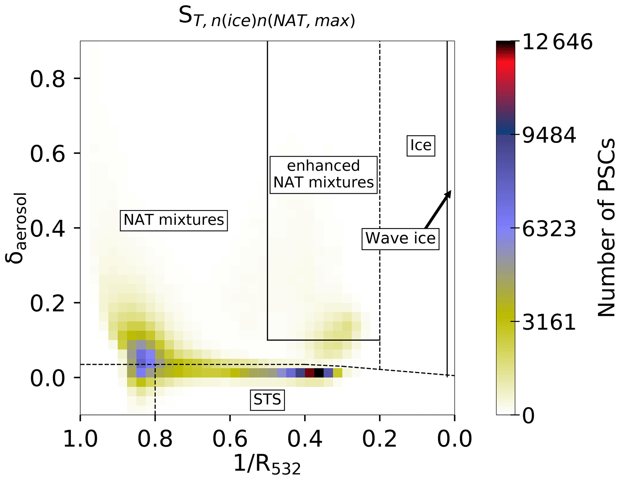
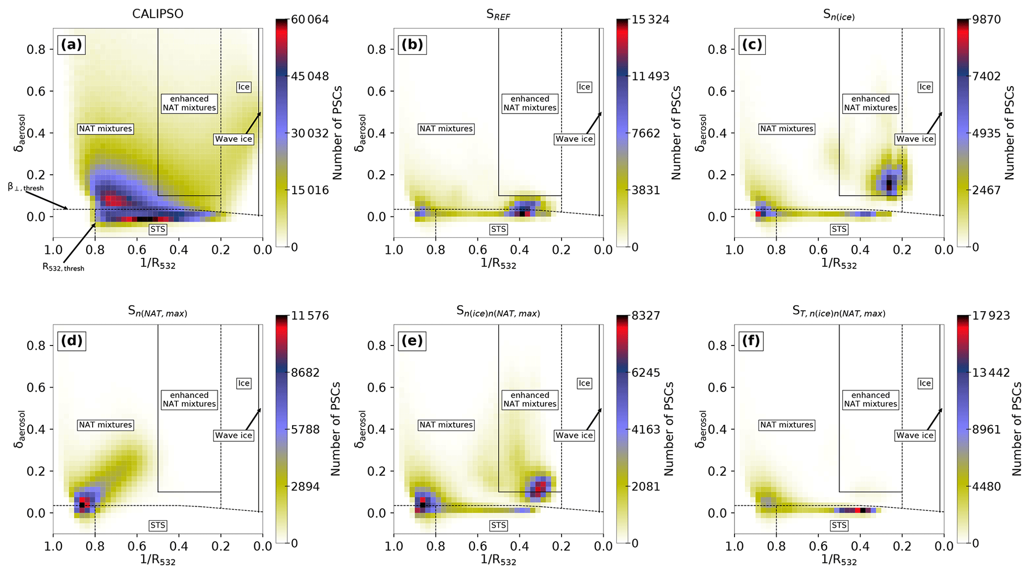
The PSC classification in Pitts et al. (2018) distinguishes STS, STS–NAT mixtures, enhanced NAT mixtures, ice and wave ice. The categories are visualized in Fig. 1. The dotted lines denote dynamical boundaries, while the solid lines show boundaries at fixed β_⟂ or R₅₃₂ values. The lines in the lower left corner approximate the β_⟂ threshold (${\mathit{\beta }}_{⟂,\mathrm{thresh}}$) and R₅₃₂ threshold (R_532,thresh). All PSCs above ${\mathit{\beta }}_{⟂,\mathrm{thresh}}$ are assumed to contain non-spherical particles. The boundary between the two NAT mixture categories and ice is calculated “dynamically”, i.e., based on cloud-free MLS measurements of HNO₃ and H₂O. PSCs are detected as wave ice when they contain non-spherical particles and if R₅₃₂>50. A detailed description of the classification scheme is given in Pitts et al. (2018). PSC observations for July 2007 (Fig. 1) show the most distinct relative maxima for STS. Two further relative maxima appear with higher δ_aerosol values, indicating solid particles. The relative maximum extending towards the upper left corner of the histogram corresponds to STS–NAT mixtures with low NAT number densities (n_NAT), while the second relative maximum extending towards the upper right corresponds to mixtures of NAT with high number densities and ice as well as to wave ice PSCs.

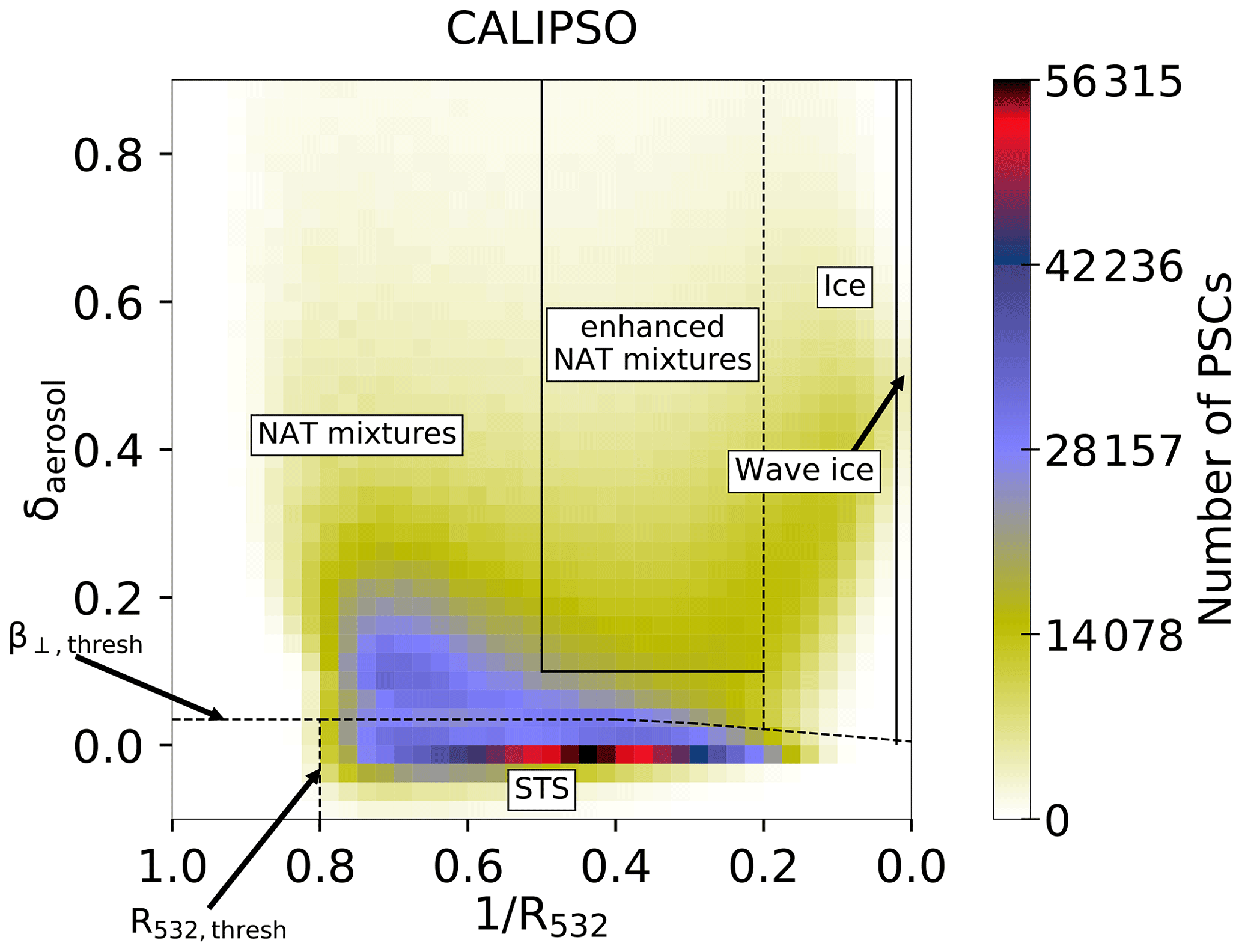
Figure 1 Composite 2D histogram of CALIPSO PSC measurements for July 2007 in a $\mathrm{1}/R_{\mathrm{532}}$–δ_aerosol coordinate system with 40×40 bins. The colors indicate the number of PSC measurements in one bin. Dotted lines denote dynamical classification boundaries or thresholds, and solid lines denote fixed classification boundaries.

2.3 MLS observations

In this study, modeled HNO₃, H₂O and O₃ mixing ratios are compared to satellite measurements of the Microwave Limb Sounder (MLS) on board the Aura satellite (Waters et al., 2006). MLS measures atmospheric profiles by scanning from the ground to 90 km of height in the flight direction, passively measuring microwave thermal emissions. All three quantities are derived by version 4.2 from the Aura MLS level 2 data (Livesey et al., 2018). The HNO₃ dataset has a vertical resolution of approximately 3–4 km, while the H₂O and O₃ datasets have a vertical resolution of 2.5 to 3 km. The accuracy of the MLS measurements is 1–2 ppbv for HNO₃ (Santee et al., 2007), 4 %–7 % for H₂O (Read et al., 2007; Lambert et al., 2007) and 8 % for stratospheric O₃ (Jiang et al., 2007). Detailed information and a precise description of the dataset can be found in Livesey et al. (2018).

2.4 Model–measurement comparison

While CALIOP measures backscatter signals and depolarization ratios, the SOCOL model provides surface area densities for STS, NAT and water ice as a function of pressure, latitude and longitude. From the outputted SADs of the three PSC types and the prescribed microphysical parameters, i.e.,  r_NAT and n_ice, as well as the growth factor for liquid aerosols we calculate the number density and/or radius for each particle type. These quantities are used in Mie and T-matrix scattering codes (Mishchenko et al., 1996) to compute optical parameters of the simulated PSCs, i.e., R₅₃₂, δ_aerosol and β_⟂, for comparison with CALIOP observations. For NAT and ice particles, circular symmetric spheroids with an aspect ratio of 0.9 are assumed. Refractive indices of 1.31 for water ice and 1.48 for NAT (Middlebrook et al., 1994) were chosen. STS and liquid particles are therefore assumed to be spherical, which corresponds to a depolarization ratio δ_aerosol=0.

The CALIOP PSC data product includes detection thresholds, R_532,thresh and ${\mathit{\beta }}_{⟂,\mathrm{thresh}}$, for each measurement. As the geographical PSC extent strongly depends on these detection limits, they have to be applied to the calculated optical properties of the simulated PSCs as well to ensure a fair comparison between model and satellite data. For this purpose, we calculated for each pressure level the daily mean thresholds over all observations.

The satellite measurements are subject to uncertainties. Even for a perfectly monodisperse PSC distribution a CALIPSO measurement would show some scatter. To ensure the best possible comparability between the model and measurements, observational uncertainties have to be applied to the calculated optical properties of the modeled PSCs. We followed the approach by Engel et al. (2013). The uncertainty scales inversely with the square root of the horizontal averaging distance along a flight path, which we set to 135 km. This value corresponds to the best case for detection, which maximizes the comparability with the model (which obviously does not have a detection threshold). An example for the added measurement noise is shown in Fig. 2. When looking at the three PSC types individually (Fig. 2a), STS (due to their assumed spherical shape) and NAT (due to the fixed radius) appear at constant δ_aerosol values of 0 and 0.167, respectively. The variable radius of ice particles results in a variable δ_aerosol value. Applying the uncertainties to the parallel and the perpendicular backscatter coefficients primarily causes a large spread in the depolarization ratio (Fig. 2b). When considering all PSC particles to be mixed within a grid box (Fig. 2c), they appear mainly in the lower and left side of the composite histogram.

Figure 2 Scatter plot of simulated PSCs from the SOCOL simulation S_REF on 1 July 2007 in a $\mathrm{1}/R_{\mathrm{532}}$–δ_aerosol coordinate system. (a) STS (red), NAT (green) and ice (blue) as individual components. (b) As in (a), but after applying observational uncertainties. (c) The modeled PSCs as mixture of all components present per grid box (red: pure STS, green: STS–NAT mixtures, blue: mixtures with ice) with uncertainty.

3 Results and discussion

Since our results and conclusions do not substantially differ for the three analyzed winters, we focus here on the year 2007, a typical Antarctic winter. Figures for the winters 2006 and 2010 are shown in the Appendix (Figs. A3–A14). We start with the analysis of our reference simulation (Table 1). The sensitivity simulations are discussed in Sect. 3.4.

3.1 Comparison along an orbit

As a first example, we evaluate the vertical profile of SOCOL-simulated PSCs, comparing to lidar measurements from the CALIPSO satellite, along specific orbital transects. Figure 3 shows a curtain of observed inverse backscatter ratios $\mathrm{1}/R_{\mathrm{532}}$ along orbit 2 on 1 July 2007 (Fig. 3a) and the corresponding PSC compositions (Fig. 3d). The observations indicate a large PSC over the Antarctic Peninsula (270–300^∘ E) and a smaller PSC over Oates Land (160–190^∘ E). Further, some tropospheric cirrus clouds were classified as PSCs. Above the Antarctic Peninsula, two distinctive regions with very small $\mathrm{1}/R_{\mathrm{532}}$ values are evident. These high backscatter ratios (R₅₃₂>50) are related to high number densities of ice particles (up to 10 cm⁻³; Hu et al., 2002), which are caused by rapid cooling rates associated with mountain-wave events. These wave ice clouds are surrounded by more synoptic-scale PSCs with lower R₅₃₂ values, which are classified as ice, STS and NAT mixtures.

Figure 3b and d show the corresponding plots for the PSCs as simulated by the SOCOL model in the respective grid boxes overflown by CALIPSO. Figure 3c and f show the same, but before detection thresholds and instrument uncertainty had been added. The model output also reveals a large PSC over the Antarctic Peninsula. However, the spatial extent of the simulated PSC is larger. The simulated backscatter ratio R₅₃₂ peaks around 6, which is substantially lower than observed. Due to the coarse resolution and the rather smooth orography in the model, SOCOL is not able to capture high ice particle number densities associated with small-scale mountain-wave events. Applying the CALIOP classification scheme to the model output results in a layer of ice PSCs located around ∼ 20 km, which is slightly higher than in the observations. The ice cloud is surrounded by NAT mixtures, while the observations indicate STS. Below those NAT mixtures, pure STS clouds occur in the model (Fig. 3f), most of which are tenuous enough such that they fully disappear after applying the optical thresholds (Fig. 3e).

The actual modeled composition (Fig. A1) shows a similar pattern as the CALIOP classification scheme but with more ice mix and less STS. This difference between the actual composition and the composition according to the CALIPSO classification scheme of SOCOL PSCs can also be seen in Fig. 2c, where most of the ice mixtures (blue) are located in the NAT mixture domain, while many NAT mixtures (green) are located in the STS domain. It should be noted that the modeled optical properties are exclusively calculated for PSCs. Tropospheric cirrus clouds treated by the model's cloud routine are therefore excluded.

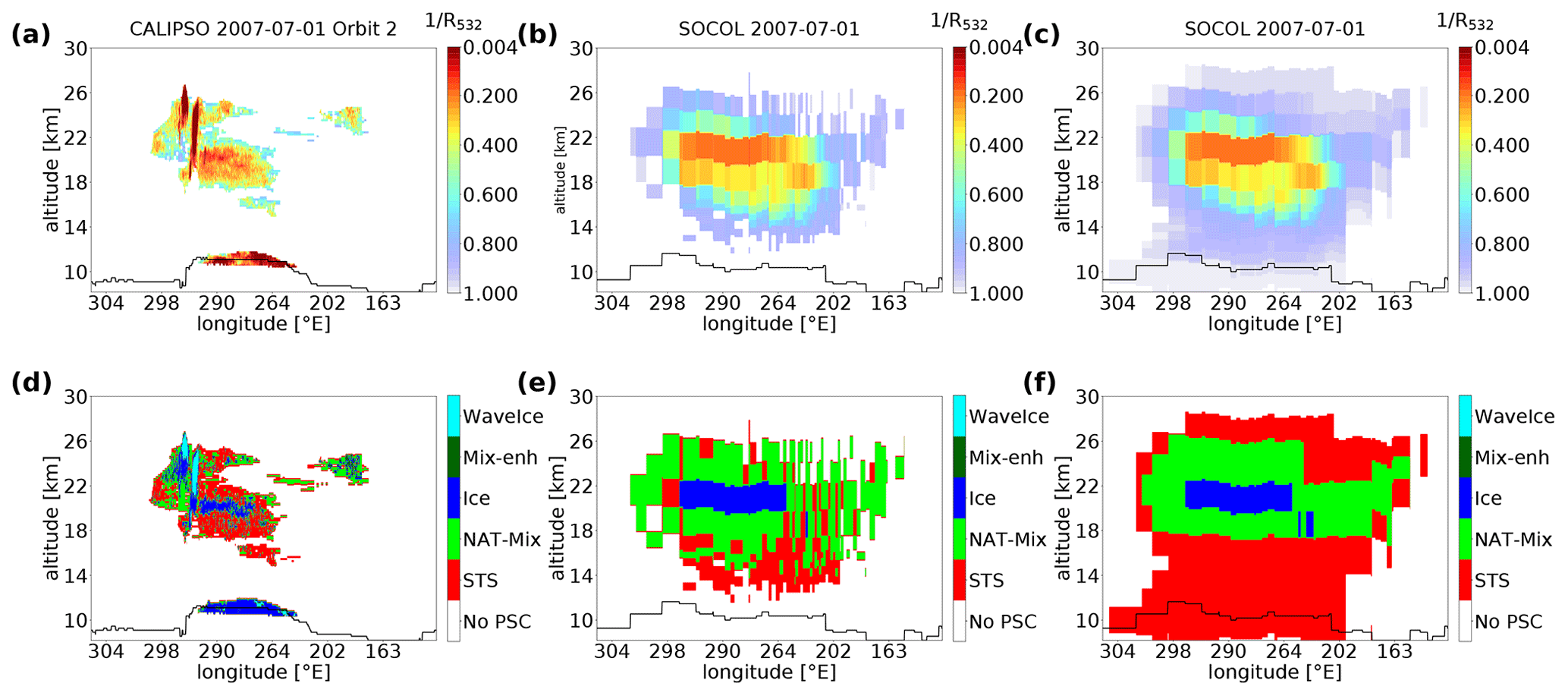
Figure 3 CALIPSO measurements on 1 July 2007 (orbit 2) of R₅₃₂ (a) and the PSC classification (d). Calculated R₅₃₂ values for modeled PSCs from the simulation S_REF in the overflown grid boxes after adding the instrument uncertainty and applying the detection thresholds are shown in (b). Panel (e) shows the composition of the corresponding PSCs according to the classification scheme in Pitts et al. (2018). (c, f) The same as in (b) and (e), but without instrument uncertainty and the detection thresholds. The black lines indicate the World Meteorological Organization (WMO) and model tropopause height for CALIPSO measurements and simulations, respectively.

3.2 Spatial distribution

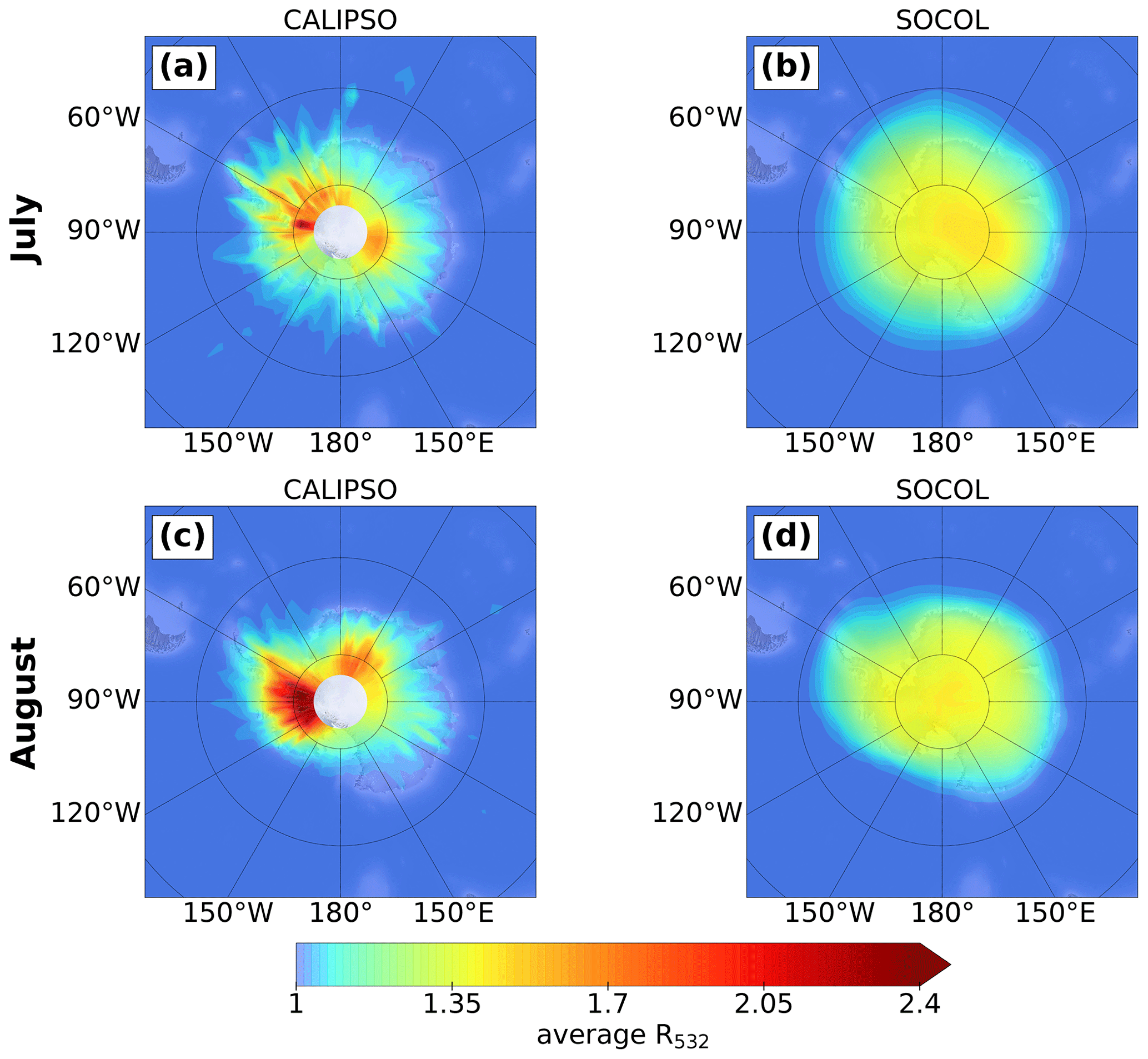
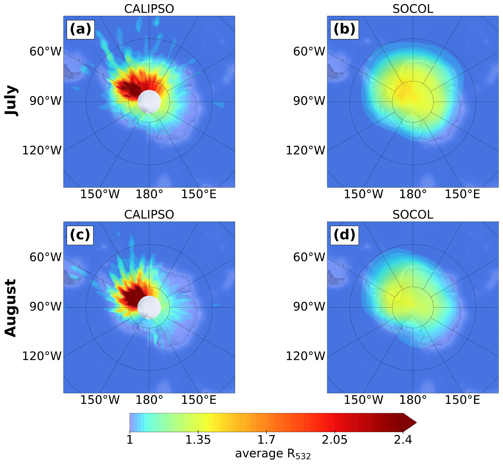
Figure 4 presents monthly mean (including clear-sky and cloudy-sky conditions) backscatter ratios R₅₃₂ from observations and the simulation for July (a and b) and August 2007 (c and d). For a better comparison, the high-resolution measurements have been gridded onto the SOCOL grid. The data are vertically averaged over all pressure levels above the tropopause. The observations show month-to-month variability in the location of the PSC region. In July, the mean backscatter intensity appears to be more homogeneously distributed, with a slight peak over East Antarctica (∼ 0–150^∘ E), while in August a distinct peak downstream of the Antarctic Peninsula (∼ 55–70^∘ W) is observed. This characteristic feature is caused by frequent mountain-wave events in this region (Hoffmann et al., 2017). These mountain waves lead to the formation of wave ice with very high backscatter values, but also to subsequent formation of enhanced NAT mixture clouds with high number densities of NAT particles (Zhu et al., 2017a).

The modeled month-to-month variability in the R₅₃₂ values and areal extent agrees well with CALIPSO observations. In July, the center of the PSC area is also tilted towards East Antarctica and slightly towards the peninsula in August. However, peak values of R₅₃₂ are clearly lower for SOCOL, and the spatial distribution is more homogeneous. As mentioned above, this results mainly from a poor representation of mountain waves in the model, but also from the fixed ice number density and upper limit for the NAT number density. Although the years 2006 and 2010 show a slightly different seasonal cycle (Figs. A5, A6), the conclusions regarding the model performance hold for those years as well.

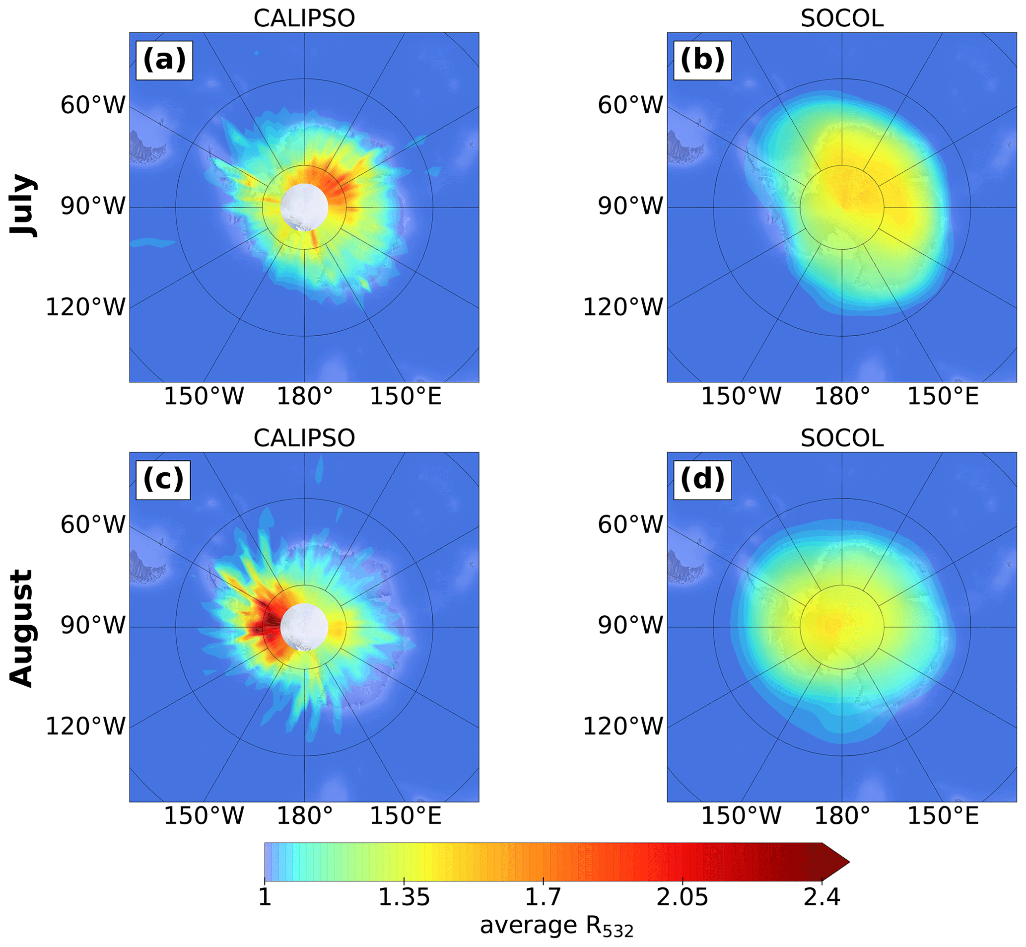
Figure 4 Vertically integrated monthly means of R₅₃₂ for all-sky conditions as observed by CALIPSO (a, c, gridded onto the SOCOL grid) and as simulated by SOCOL from the simulation S_REF (b, d) for July (a, b) and August 2007 (c, d).

3.3 PSC areal coverage

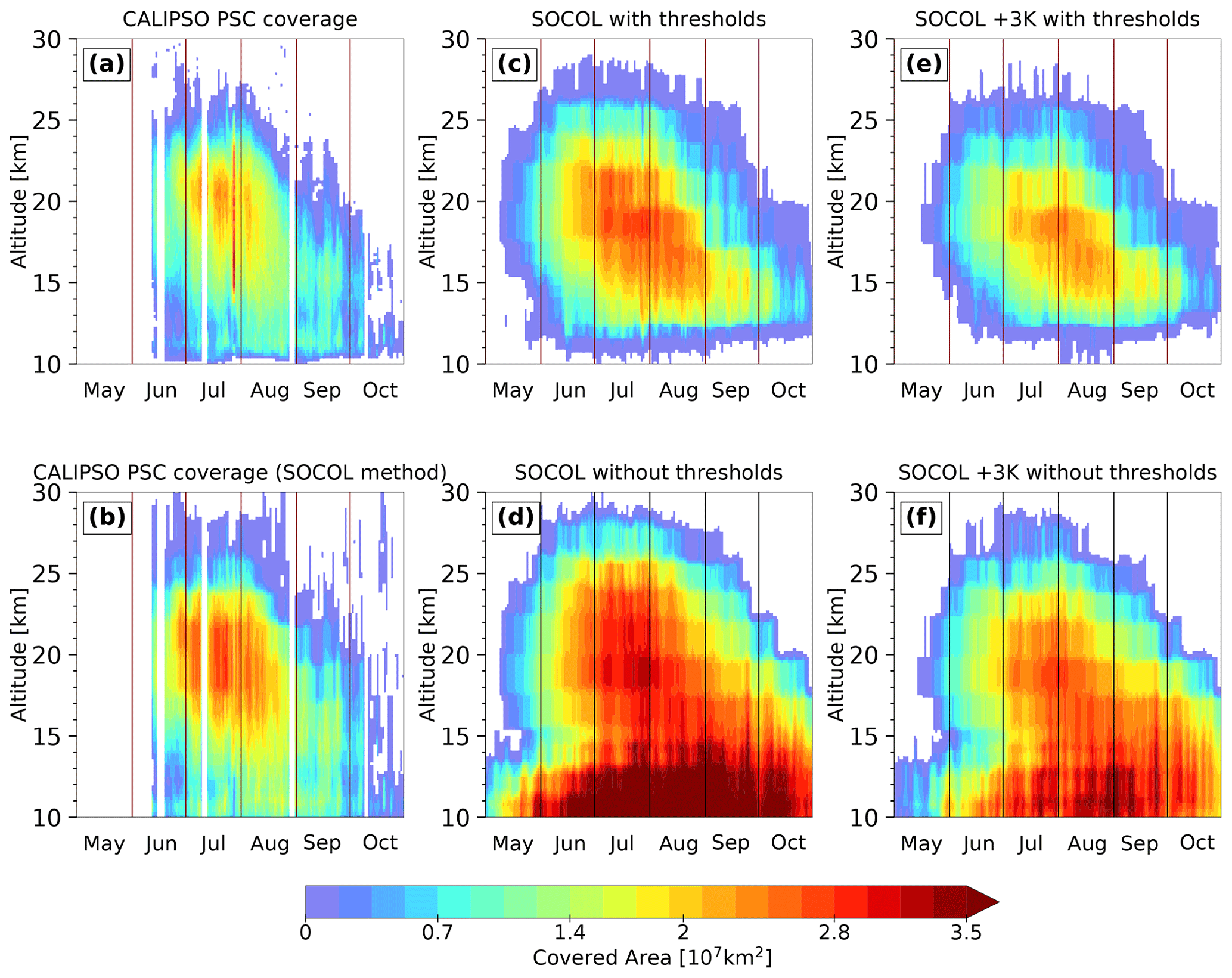
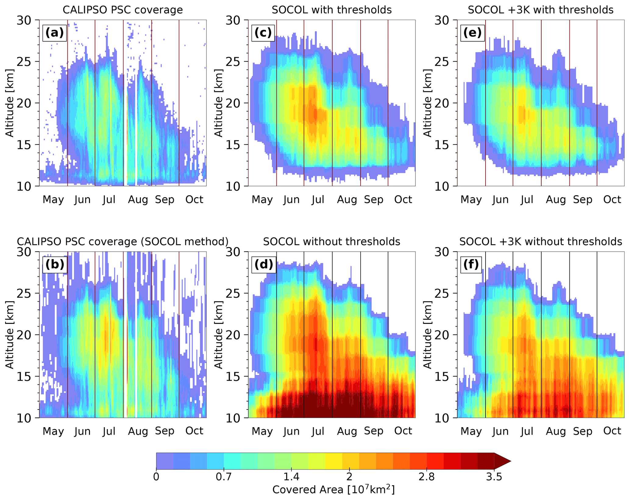
The total areal coverage as a function of altitude and time is a measure of the seasonal evolution of PSCs inside the polar vortex. Figure 5 compares CALIOP observations and model results for the winter 2007 (see also Fig. 13 in Pitts et al., 2018). The modeled PSC area is determined for every grid box based on the PSC occurrence for two output time steps per day at 00:00 and 12:00 UTC. We consider the entire model grid box to be covered by PSCs as soon as PSCs occur and exceed the detection limits. The observed PSC area is calculated in two different ways: (1) from the daily fraction of PSC measurements within 10 equally sized latitude bands, as described in Pitts et al. (2018) (Fig. 5a), and (2) from measurements averaged over 12 h and gridded onto the SOCOL grid (Fig. 5b). The second method is similar to the calculation of the modeled PSC area (the “SOCOL method”). Since CALIOP does not overpass all SOCOL grid cells within 12 h, the “empty” grid cells are filled by the PSC area in the overpassed grid cells at the same latitude. We applied the SOCOL method to the CALIOP data to achieve the best possible comparability between the model and observations. Compared to Fig. 5a, the SOCOL method leads to an increase in the CALIOP PSC areal coverage. Since CALIOP does not provide data poleward of 82^∘, measurements between 77.8 and 82^∘ S are assumed to be representative of the entire 77.8–90^∘ S latitude band.

Considering the low-level (11–12 km) clouds in May and June to be tropospheric cirrus, the first PSC occurrence is observed in mid-May at 20–25 km of altitude (Fig. 5a). Periods with higher PSC areal coverage and a large vertical extent alternate with periods of less PSC extent. A clear peak occurs at the end of July between 17 and 23 km of altitude. The PSC areal coverage starts to decrease at the beginning of September, reaching zero in mid-October. The descent of the coldest temperatures within the winter season is reflected in the decrease in PSC occurrence. As described in Pitts et al. (2018), the PSCs merge with tropospheric cirrus clouds in mid-July.

In SOCOL, PSC formation starts about 2 weeks earlier (Fig. 5c). The model is capable of reproducing the temporal occurrence of the individual peaks at the end of July. Also, the overall decrease in maximum PSC coverage is present in the simulation. PSCs exist until the end of October, which is longer than observed. Furthermore, SOCOL simulates a substantially larger PSC area than observed (Fig. 5a), in particular between 13 and 23 km of altitude, where 1.5×10⁷ km² is almost continuously exceeded.

There are two main reasons for the overestimated PSC area and for the longer PSC period in the model. Part of the overestimation can be explained by the calculation method, since even small numbers of PSCs within a large model grid cell substantially contribute to the PSC areal coverage. However, SOCOL still overestimates CALIPSO when applying the SOCOL method to the observations (Fig. 5b). Most of the overestimation results from a cold temperature bias in the polar lower stratosphere, which is typically around 2 to 4 K. Offsetting this cold bias by +3 K in a sensitivity simulation results in a decrease in the simulated PSC areal coverage (Fig. 5e) and clearly improved agreement with CALIOP observations (Fig. 5b).

The modeled PSC area calculated without the optical thresholds applied (Fig. 5d and f) is significantly larger, especially below 13 km of altitude, where large areas with STS clouds occur in the model (see also Fig. 3f). Those large-scale STS clouds are very tenuous and filtered out by applying the conservative PSC detection threshold. The contribution of those STS clouds to SAD is negligible. However, the comparison highlights the crucial role of the detection thresholds for model–measurement intercomparisons. Due to this sensitivity to the applied methods, quantitative comparisons of the areal coverage must be interpreted with caution.

Observed and simulated PSC coverage for the years 2006 and 2010 are shown in Figs. A5 and A6. In 2006, the year with above-average PSC occurrence, offsetting the cold bias leads to a smaller PSC coverage than observed, indicating that not the synoptic-scale temperature, but rather small-scale temperature fluctuations, determined the PSC occurrence and areal coverage in 2006 (see also Fig. A3). As such small-scale features are not adequately represented in SOCOL, correcting for the synoptic-scale temperature bias leads to an underestimation of the PSC coverage.

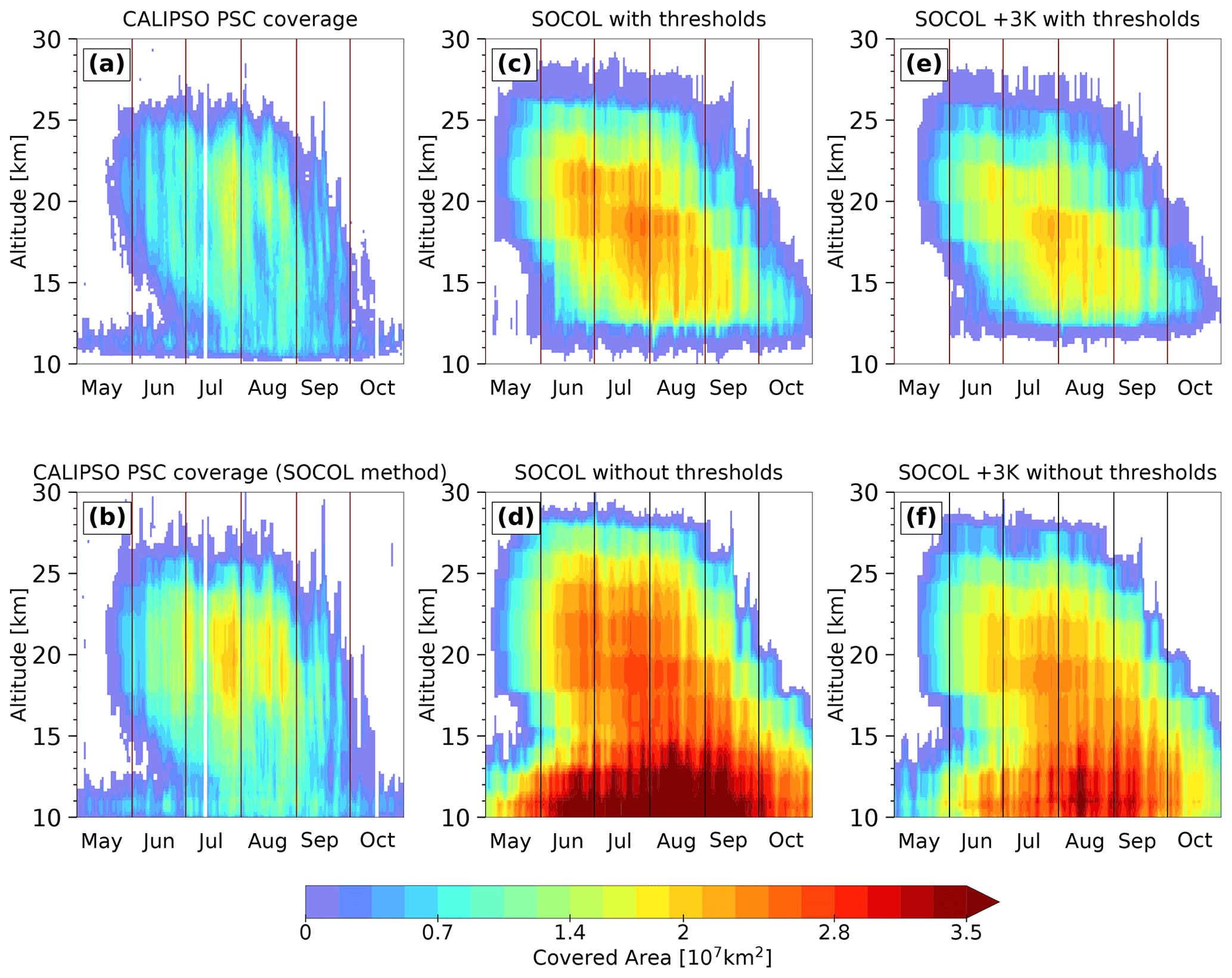
Figure 5 Time series of total PSC areal coverage over the Antarctic region as a function of altitude for winter 2007. Panel (a) is derived from CALIOP as described in Pitts et al. (2018). Panel (b) is derived from CALIOP by applying the SOCOL method (see text). Panels (c) and (d) are derived from the SOCOL reference simulation with and without applying detection limits and instrument uncertainty, respectively. Panels (e) and (f) are the same as for (c) and (d), but with PSC formation temperature increased by 3 K.

3.4 Sensitivity to microphysical parameters

As described in Sect. 2.1, SOCOL's PSC scheme includes some prescribed microphysical parameters such as the ice particle number density, n_ice, and the NAT radius, r_NAT. The values used for such PSC microphysics parameters tend to inherit early choices based on initial comparisons with limited observational datasets. Also, the initial parameter values chosen may reflect specific conditions in a particular polar winter and may require adjustment to be more representative over the broader range of conditions experienced across several winters. For example, the value for n_ice of 0.01 cm⁻³ prevents the formation of ice PSCs with high number densities as observed in mountain-wave events. To investigate the sensitivity of the simulated PSCs to the parameter setting, we performed additional simulations with increased n_ice and/or increased n_NAT,max (Table 1). In addition, we performed a simulation with increased temperatures for PSC formation to investigate the effect of the cold temperature bias on simulated PSCs and chemical composition within the polar vortex.

Table 1 Overview of the SOCOL simulations and the microphysical parameter settings. The parameters deviating from the reference setting are denoted in bold.

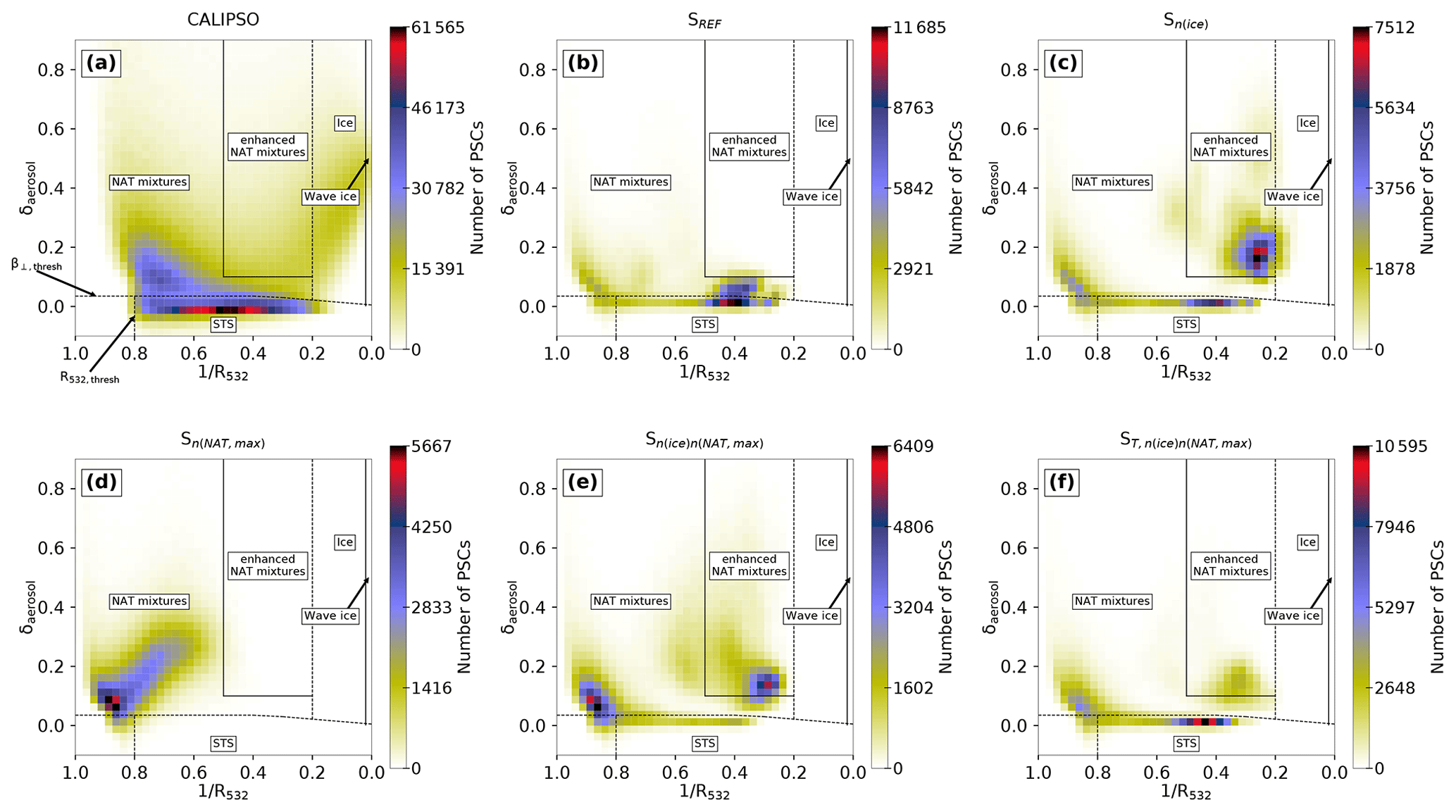
Figure 6 shows the composite histograms for various SOCOL simulations. There are considerable differences to the observations (Fig. 1), but also between the simulations. PSCs in the reference simulation S_REF show a strong relative maximum located in the STS domain with $\mathrm{1}/R_{\mathrm{532}}$ values between 0.4 and 0.2 (Fig. 6a). Very few PSCs are classified as ice; i.e., the relative maximum towards the upper right, as observed by CALIPSO, is missing. The shift of modeled PSC towards the lower and left side of the histogram is also visible in Fig. 2c. There are several reasons for this difference: first, SOCOL does not resolve small-scale mountain waves due to the coarse horizontal resolution and smooth orography applied in the model. Furthermore, the modeled PSCs are representative of a large grid box (2.8^∘ × 2.8^∘ horizontally and approximately 2 km vertically), while the observations resolve much smaller-scale structures (starting from 5 km horizontally along a track and 180 m vertically). Finally, the fixed ice number density of 0.01 cm⁻³ and upper limit for NAT number densities do not allow for large ice and NAT cross sections, even if mountain waves were resolved. Based on these findings we performed one sensitivity simulation with a 10-fold ice number density, S_n(ice). As shown in Fig. 6b the 10-fold increase in n_ice results in a strong maximum towards the upper right, mainly within the enhanced NAT mixture domain. The higher number density of ice particles increases the cross section of ice, leading to enhanced backscatter in ice-containing grid cells. Due to its solid state, backscatter from ice has δ_aerosol>0. This results in a shift towards higher R₅₃₂ and higher δ_aerosol values in the histogram. Overall, modifying n_ice leads to better agreement in optical properties with CALIPSO.

NAT PSCs play a twofold role in stratospheric ozone chemistry: besides efficient halogen activation on their surfaces, the sedimentation of NAT particles leads to denitrification, which hinders deactivation of reactive halogens and facilitates catalytic ozone loss (Peter, 1997). While ice PSCs are less important for stratospheric ozone chemistry, NAT formation and subsequent denitrification of the stratosphere play a crucial role. NAT formation in SOCOL depends on two parameters, n_NAT,max and r_NAT. To test the model's sensitivity to those parameters, we ran further simulations with the upper boundary for NAT number densities increased by a factor of 4, S_n(NAT,max), and the NAT radius increased from 5 to 7 µm. As both simulations showed similar changes, the latter is not presented here.

The simulation with 4 times higher n_NAT,max (Fig. 6c) shows a maximum shifted towards lower R₅₃₂ values compared to the REF simulation, which is located around the optical thresholds in the lower left corner. As long as temperatures are below T_NAT and enough HNO₃ is available for NAT formation, an increase in n_NAT,max or r_NAT results in more HNO₃ uptake by NAT particles. This reduces the available gas-phase HNO₃ for STS growth. Also, more HNO₃ through sedimentation of the solid NAT particles is removed. With larger r_NAT this removal occurs even faster due to the higher sedimentation velocity. The reduction in surface area density of STS results in less backscatter and subsequently a shift towards lower R₅₃₂ values in the composite histogram. This shift towards lower R₅₃₂ values worsens agreement with observations.

In a further simulation ($S_{n\left(\mathrm{ice}\right),n(\mathrm{NAT},\max )}$, Fig. 6d) we set n_ice to 0.05 cm⁻³ and n_NAT,max to 10⁻³ cm⁻³. This simulation shows a superposition of the two effects described above, resulting in two distinct relative maxima in the composite histogram. One maxima is located to the upper right, similar to S_n(ice). The second maximum at low R₅₃₂ and low δ_aerosol values is similar to the pattern in S_n(NAT,max). The shift towards lower R₅₃₂ values is again a result of less STS formation due to the reduced availability of HNO₃. Although the composition histograms of all sensitivity simulations still differ substantially from the observations, we find the best agreement for the simulation $S_{n\left(\mathrm{ice}\right),n(\mathrm{NAT},\max )}$. Similar shifts in the composite plots between the various model simulations as discussed above can be found for 2006 and 2010 (Figs. A7 and A8). In the model simulation $S_{T,n\left(\mathrm{ice}\right),n(\mathrm{NAT},\max )}$ including a cold bias correction of +3 K (Fig. A2) the synoptic-scale temperatures are too warm for substantial ice formation, emphasizing the importance of small-scale temperature fluctuations for ice PSCs.

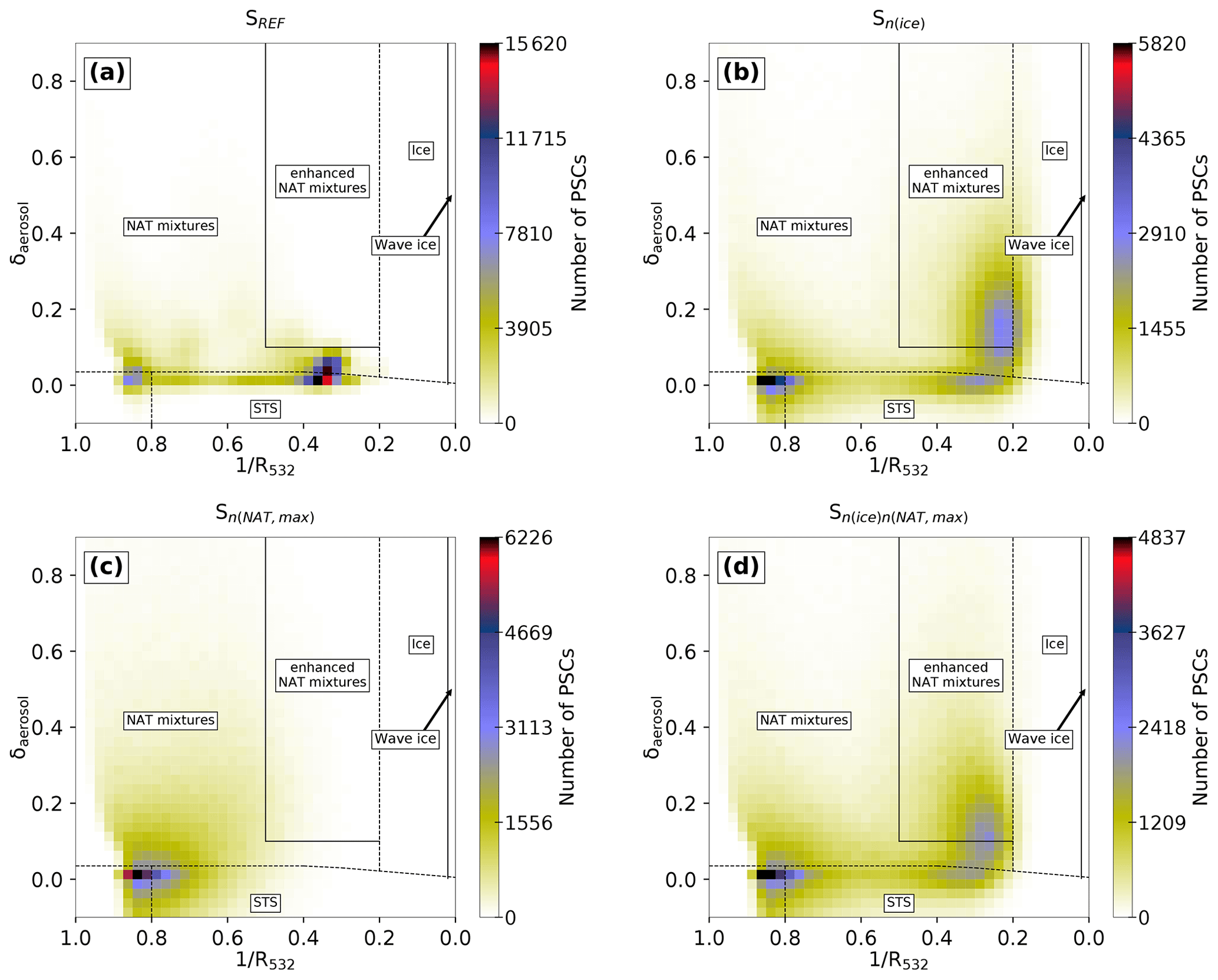
Figure 6 Composite 2D histograms for July 2007, analogous to Fig. 1, for the simulations S_REF (a), S_n(ice) (b), S_n(NAT,max) (c) and $S_{n\left(\mathrm{ice}\right),n(\mathrm{NAT},\max )}$ (d).

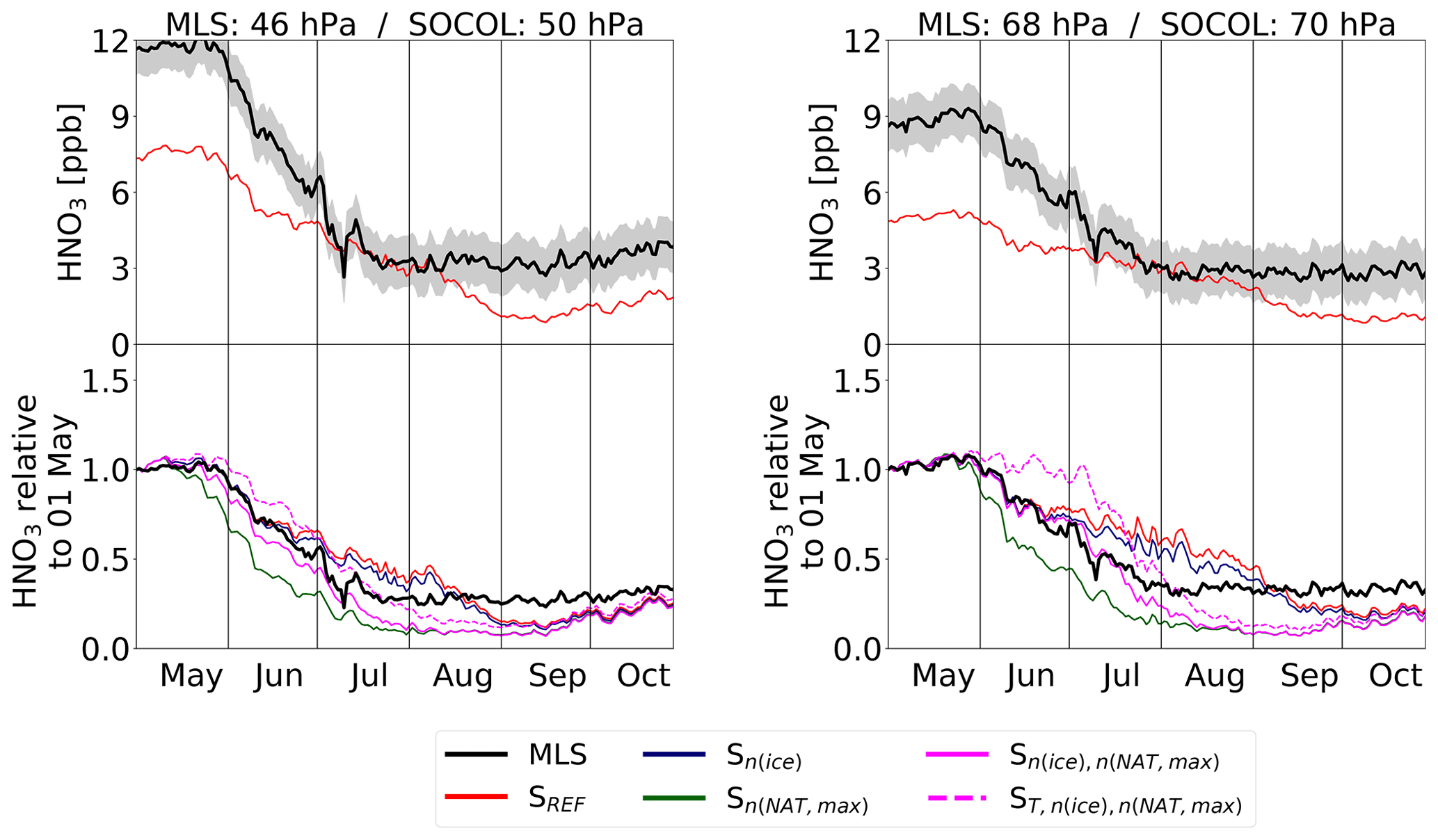
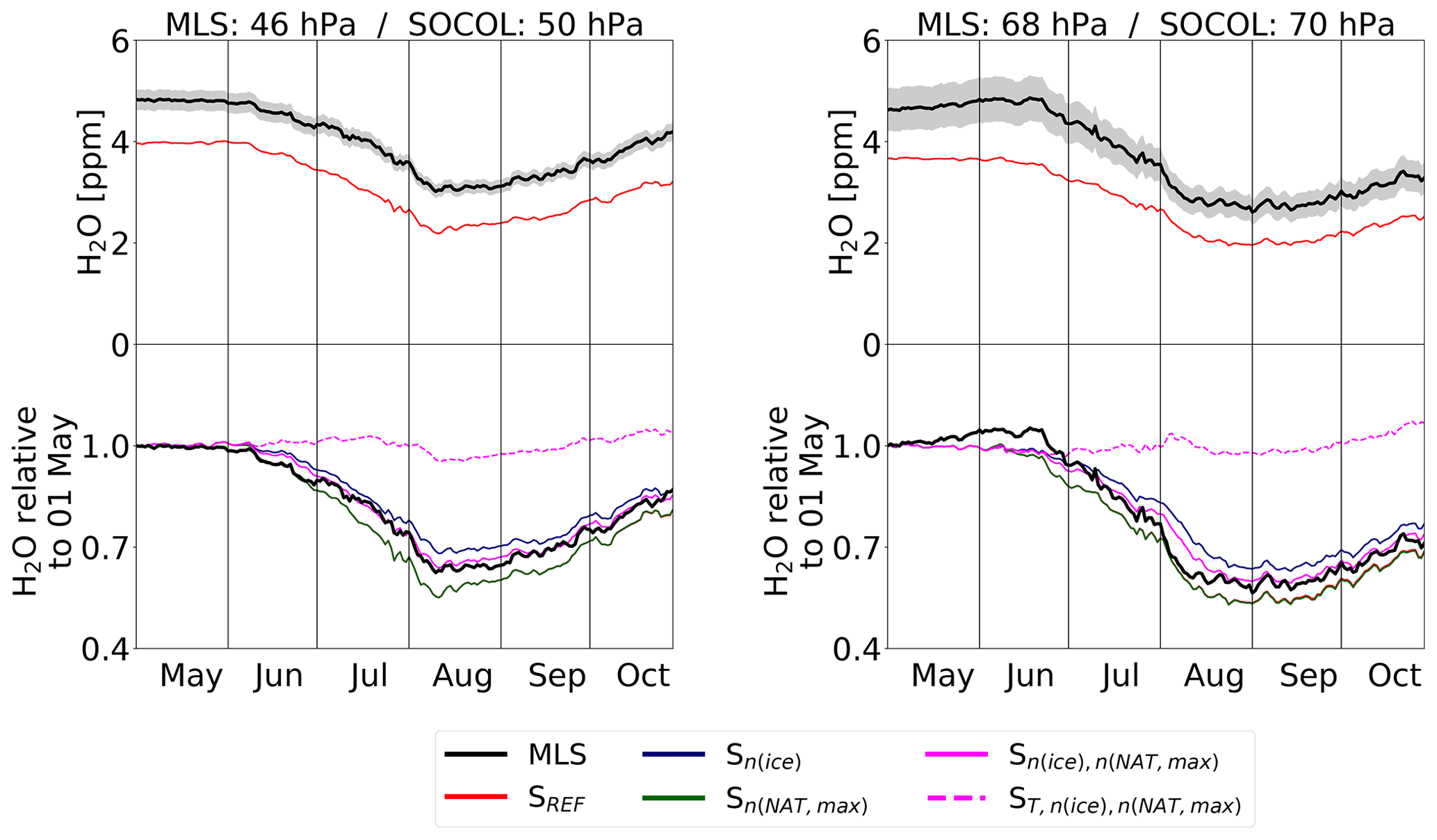
To investigate the impact of the applied modifications on the simulated chemical composition of the polar stratosphere (60–82^∘ S), we compare modeled gas-phase HNO₃, H₂O and O₃ with MLS measurements for 46 and 68 hPa (Figs. 7–9). To account for the spatial heterogeneity of the MLS measurements, we first averaged the measurements over the SOCOL grid boxes. Afterwards we calculated area-weighted polar mean concentrations. The top panels shows absolute values for MLS and the S_REF simulation, while the lower panels show the temporal evolution for MLS and all model simulations relative to 1 May.

At the beginning of winter, all simulations have similar HNO₃ concentrations, which are about 20 % to 50 % lower than MLS, depending on the pressure level (Fig. 7). At 46 hPa MLS HNO₃ starts to decline around mid-May and in early June at 68 hPa. Prior to the decline, an increase in HNO₃ is observed at 68 hPa. This results from the evaporation of sedimenting NAT particles formed at higher altitudes (renitrification) and is an indication of denitrification of the upper levels. During July–August the absolute HNO₃ values from the reference run S_REF agree well with the observations. However, in late winter SOCOL again underestimates HNO₃ compared to MLS. All simulations show a decline due to HNO₃ uptake into NAT particles and STS droplets. However, S_REF (red) and S_n(ice) (dark blue) show a weaker and delayed HNO₃ decline with a plateau in July–August.

In S_n(NAT,max) (green) the decline at both levels is considerably stronger than in S_REF and MLS. This is due to the enhanced uptake of HNO₃ into NAT particles and the subsequent removal by sedimentation. As a consequence the renitrification at lower levels is also clearly enhanced. Both features indicate greater denitrification in the increased n_NAT,max run (sensitivity run S_n(NAT,max)) than in S_REF.

The simulation $S_{n\left(\mathrm{ice}\right),n(\mathrm{NAT},\max )}$ (magenta), in which n_NAT,max is twice as large as in S_REF but only half of S_n(NAT,max), falls between the other simulations. The denitrification starts about half a month later than in S_n(NAT,max). The HNO₃ uptake is reduced and subsequently HNO₃ stays in the gas phase longer. However, in August HNO₃ concentrations reach about the same level as in S_n(NAT,max). Simulations with enhanced r_NAT have similar effects (not shown).

In $S_{T,n\left(\mathrm{ice}\right),n(\mathrm{NAT},\max )}$ denitrification and renitrification are delayed by about half a month due to the later onset of PSC formation. However, towards the end of the winter, HNO₃ concentrations are almost the same in all model simulations.

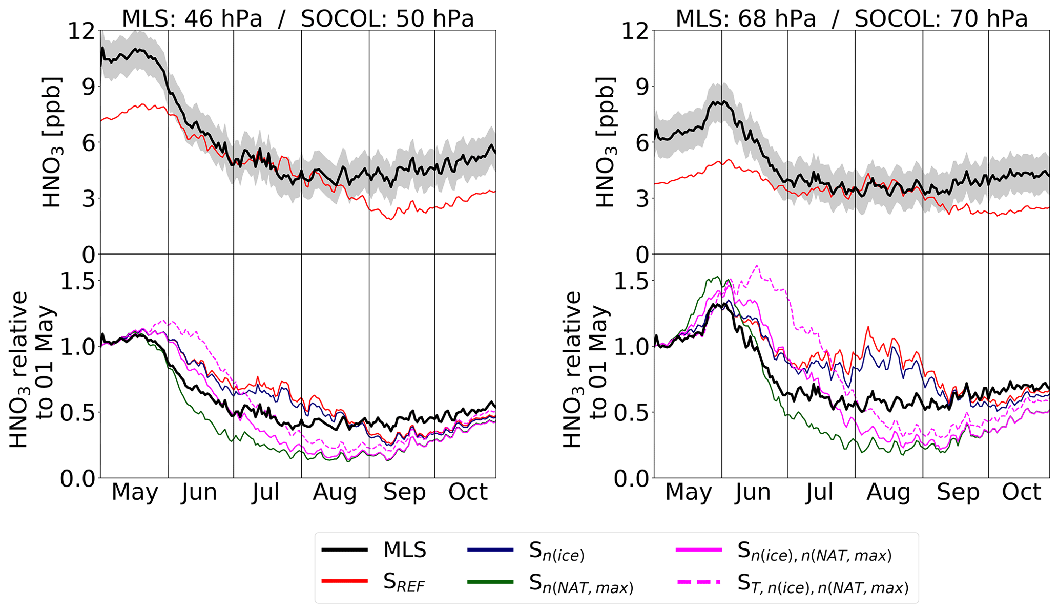
Figure 7 Temporal evolution of polar (60–82^∘ S) mean gas-phase HNO₃ from MLS measurements and the different model simulations. The uncertainty range (gray shading) represents the MLS accuracy.

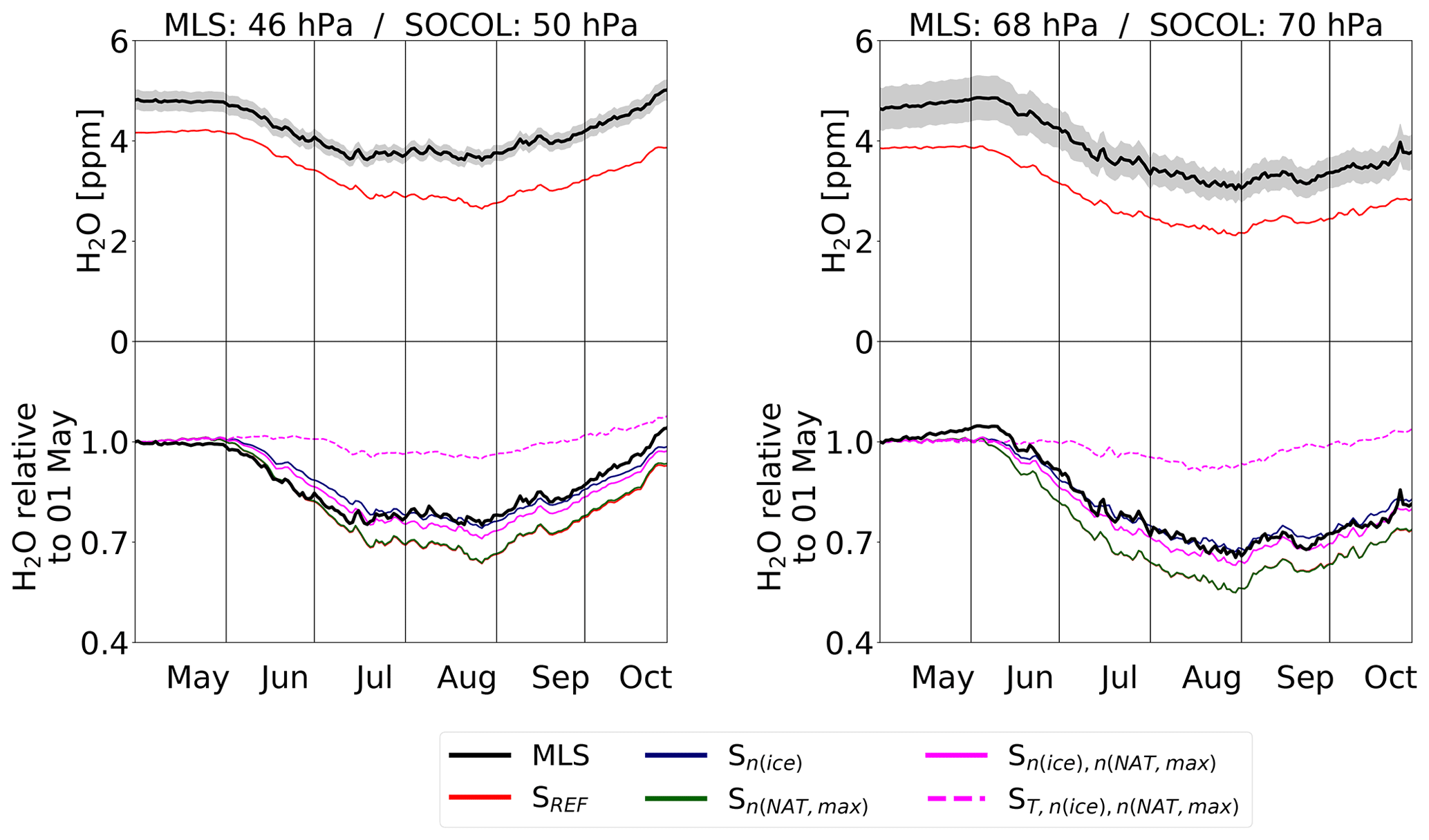
Figure 8 shows the same as Fig. 7, but for H₂O. As for HNO₃, all simulations start with similar H₂O values in May but underestimate MLS by 20 % to 30 %. At 46 hPa MLS H₂O starts to decline at the beginning of June. Rehydration of lower levels due to the evaporation of sedimenting ice particles is observed shortly after. At 68 hPa, MLS H₂O starts to decrease in mid-June. All model simulations except for $S_{T,n\left(\mathrm{ice}\right),n(\mathrm{NAT},\max )}$ show a very similar temporal evolution of H₂O in the polar stratosphere and very good agreement with MLS. In SOCOL the amount of ice is determined by the amount of available H₂O and temperatures. The smaller the chosen n_ice, the larger the ice particles and the stronger the dehydration due to faster sedimentation. S_REF and S_n(NAT,max), the simulations with the lowest n_ice of 0.01 cm⁻³, show the strongest dehydration and the earliest onset, while S_n(ice) with n_ice=0.1 cm⁻³ shows the smallest dehydration of the simulations without a modified PSC formation temperature. With the cold bias correction of +3 K, almost no dehydration takes place due to lack of ice formation. Changes in polar vortex H₂O from modifying n_ice have an influence on the SAD of NAT and STS, with higher H₂O concentrations leading to larger NAT and STS SADs. However, this effect is small compared to the effects of modifying the NAT-related microphysical parameters and is therefore not discussed further.

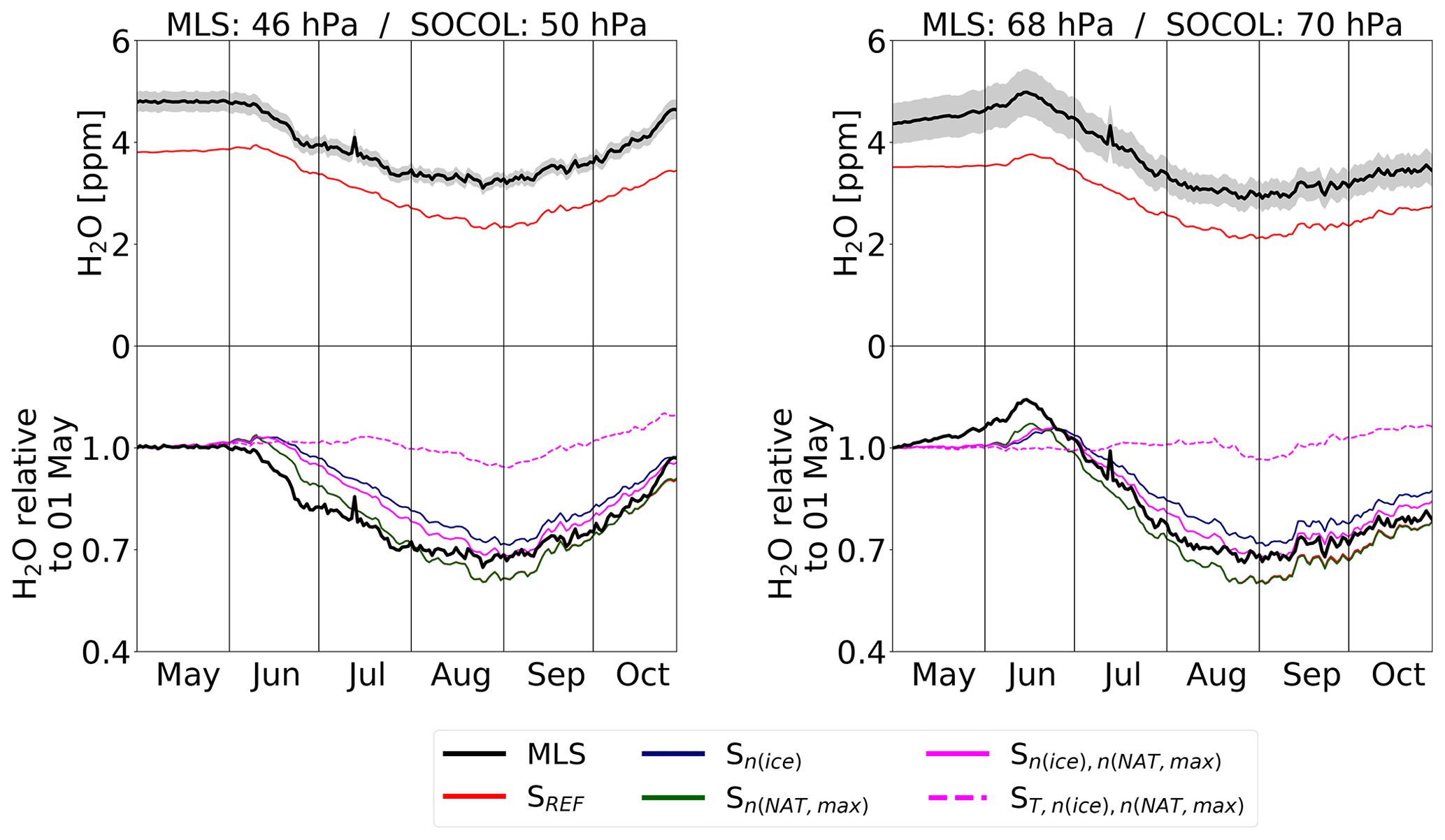
Figure 8 Same as Fig. 7, but for H₂O. Note that the line of S_n(NAT,max) overlays S_REF, since these simulations have identical H₂O.

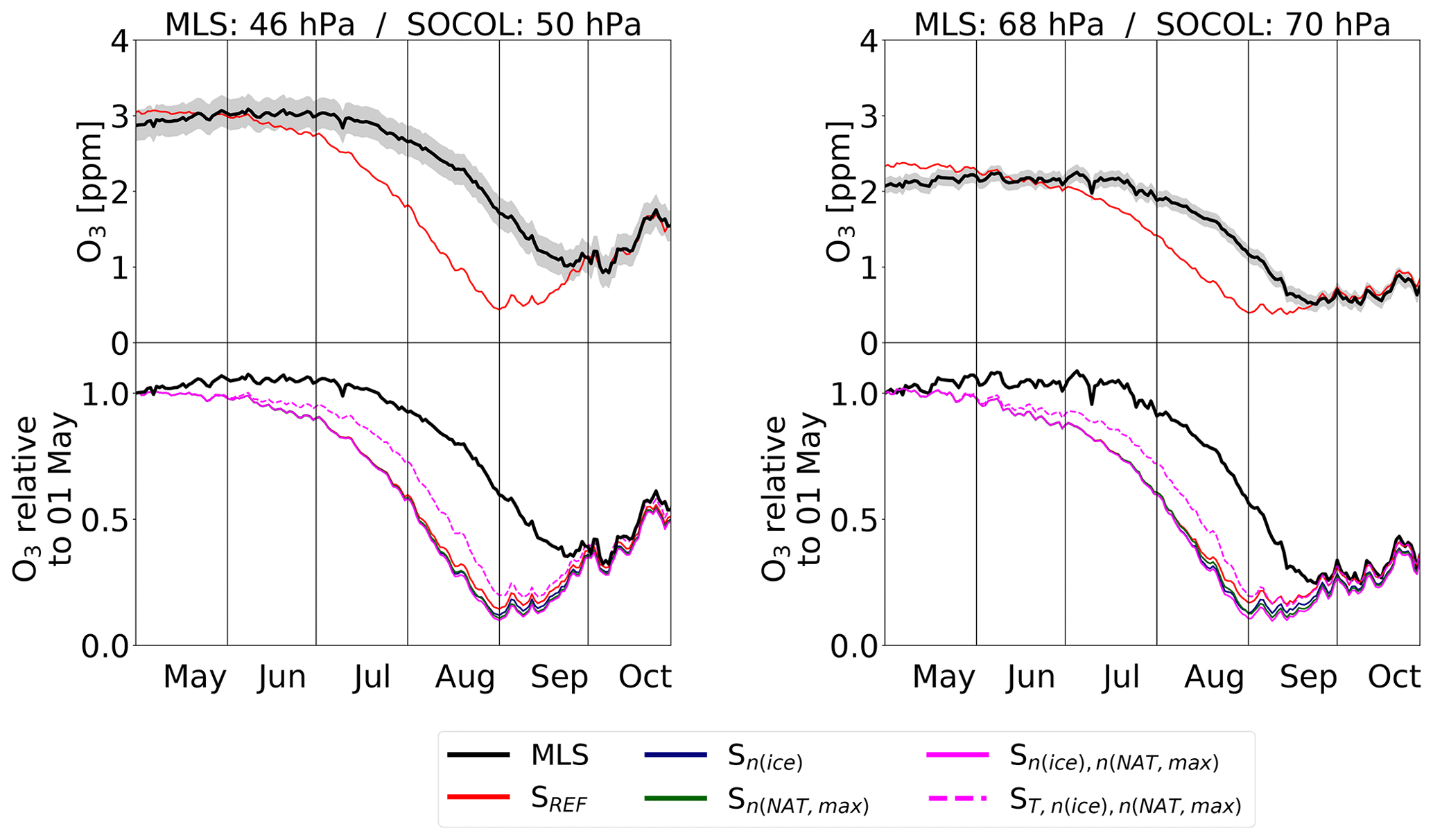
Finally, Fig. 9 presents simulated O₃ in the polar stratosphere compared to MLS. At the beginning of winter all model simulations are in very good agreement with MLS measurements. For both pressure levels, the simulations show an earlier and stronger decline in O₃ than observed by MLS. Also, the recovery of O₃ starts earlier, leading to slightly higher O₃ values at the end of October. The spread among the model simulations is small compared to the differences to the observations, indicating minor effects of the PSC parameters on O₃depletion. Increasing the parameter n_ice slightly reduces the simulated dehydration, but the increased SAD of ice leads to a slightly stronger O₃ depletion in S_n(ice) compared to S_REF. Allowing for higher NAT number densities overall reduces SAD of PSCs due to reducing the abundance of HNO₃. However, due to enhanced denitrification, S_n(NAT,max) and $S_{n\left(\mathrm{ice}\right),n(\mathrm{NAT},\max )}$ even show slightly lower O₃ concentrations. O₃ depletion starts later in $S_{T,n\left(\mathrm{ice}\right),n(\mathrm{NAT},\max )}$ due to the later onset of PSC occurrence and smaller PSC area. However, from the end of August onwards the differences between the individual model simulations vanish. The discussed findings for HNO₃, H₂O and O₃ also hold for the years 2006 and 2010, as shown in Figs. A11 to A14.

Figure 9 Same as Fig. 7, but for O₃.

4 Discussion and conclusions

We have presented an evaluation of polar stratospheric clouds (PSCs) in the Antarctic stratosphere as simulated by the chemistry–climate model SOCOLv3.1. The model was nudged towards ERA-Interim reanalysis (specified dynamics mode). We evaluated modeled PSC occurrence and composition compared to CALIPSO and CALIOP satellite observations by deriving an equivalent backscatter metric from the model output and aligning with optical thresholds used in the CALIOP classification algorithm. The impact of PSCs on the chemical composition of the polar stratosphere by denitrification, dehydration and ozone depletion was investigated by comparison with Aura/MLS satellite data. We analyzed three winters with different PSC occurrence: 2006 (above average), 2007 (average) and 2010 (below average).

SOCOL considers STS droplets as well as water ice and NAT particles. PSCs are parameterized in terms of temperature and partial pressures of HNO₃ and H₂O, assuming equilibrium conditions. In the model, NAT and ice PSCs form instantaneously, whereas NAT particles are known to require several days to grow to larger sizes, their size then being dependent on the history of the air mass. The instantaneous NAT formation approach therefore represents a simplification, but it has been successfully applied in several other models (e.g., Wegner et al., 2013) and evaluated against PSC schemes resolving the time required for growth (e.g., Feng et al., 2011).

The simplified PSC scheme then requires us to assign representative constant values for several PSC microphysics parameters, namely the maximum NAT number density, NAT radius and ice number density. Fixing the NAT radius leads to a homogeneous sedimentation velocity for all NAT particles but allows for varying NAT number densities. Other models choose the reverse approach with fixed number densities, which results in varying NAT radius and sedimentation velocities (e.g., Wegner et al., 2013; Nakajima et al., 2016). In reality, the NAT number density is far from constant because of different cold-pool and vortex situations (e.g., Mann et al., 2003), with the availability of NAT nuclei (Voigt et al., 2005) themselves showing a wide distribution of efficacies (Hoyle et al., 2013; James et al., 2018). Both approaches require some testing to reach representative microphysical parameter values that reasonably simulate observed sedimentation and denitrification. In this study, we have explored the implications of some of the values chosen in the simplified PSC scheme by analyzing several sensitivity simulations and progressing to new values, which we show perform reasonably well across the broader conditions found across several Antarctic winters.

Overall, the spatial distribution of modeled PSCs is in reasonable agreement with CALIOP observations, and the model captures the observed month-to-month variability. However, due to the coarse model resolution and mean orography, but also due to the fixed ice number densities and upper limit for NAT number densities, mountain-wave-induced ice and enhanced NAT clouds with high backscatter ratios, mainly observed over the Antarctic Peninsula, are not resolved by the SOCOL model. The PSC areal coverage over Antarctica indicates a continuous overestimation of PSCs in SOCOL. As shown by a sensitivity simulation, this can be partly explained by the simulated cold temperature bias in the winter polar stratosphere, which prevails despite running the model in specified dynamics mode. Furthermore, it is a consequence of the large grid size: even a small number of PSCs within a grid cell adds a large contribution to the areal coverage.

The choice of the prescribed ice number density, n_ice, primarily determines the optical signal and dehydration of the polar vortex through its impact on the particle size and therefore sedimentation velocities. While increasing n_ice from the original value of 0.01 to 0.1 cm⁻³ improves the agreement of the optical signal with CALIOP measurements, the simulated dehydration is more realistic for smaller n_ice and therefore larger ice particles.

The upper limit for NAT number densities determines the HNO₃ uptake and subsequently the competition between simulated NAT and STS formation, which is crucial for halogen activation. Increasing the maximum NAT number densities improves the temporal agreement of denitrification and renitrification with MLS measurements. However, SOCOL clearly underestimates observed HNO₃ in the polar stratosphere before the PSC season, which makes a solid conclusion about the best set of microphysical parameters difficult. Despite stratospheric H₂O and in particular HNO₃ being very sensitive to changes in the microphysical parameters, we found the impact on O₃ depletion to be surprisingly small.

Eliminating the cold temperature bias inside the polar vortex has a more pronounced impact on O₃ concentrations. The onset of O₃ depletion is delayed by 1 to 2 weeks. However, the maximum O₃ decline in September is overestimated by all model simulations compared the MLS. This suggests either heterogeneous ozone loss in the SOCOL model that is too strong or shortcomings regarding the model's dynamics inside the polar vortex. The latter was discussed by Khosrawi et al. (2017) as a potential reason for the underestimated polar vortex ozone concentrations in the EMAC chemistry–climate model. Brühl et al. (2007) found that, even in specified dynamics mode, the downward transport in the lower part of the polar vortex is too weak. Since the SOCOL model is based on the same general circulation model as EMAC, the underestimated polar stratospheric ozone concentrations in SOCOL are not necessarily exclusively caused by chemical ozone destruction that is too strong, but they could also be related to downward transport that is too weak, diminishing the re-supply with ozone-rich air masses from higher altitudes. This would explain why polar stratospheric ozone in the SOCOL model is shown to be rather insensitive to modifications in the PSC scheme.

The co-existence of NAT and STS poses a substantial challenge to PSC parameterizations. As mentioned above, the SOCOL model addresses this issue by setting an upper limit for NAT number densities. Khosrawi et al. (2017, 2018) found underestimated PSC volume densities as well as denitrification and renitrification in the Arctic polar vortex simulated by the chemistry–climate model EMAC. The authors explained these findings with an unrealistic partitioning of gas-phase HNO₃ into STS and NAT, with NAT forming first at the expense of STS, the main contributor to PSC volume density. In addition, the simulated NAT particles may be too small for significant gravitational settling and renitrification of lower atmospheric levels. Khosrawi et al. (2018) suggested an adjusted HNO₃ partitioning and/or an upper limit for NAT number densities, as applied in the SOCOL model, as one potential way to improve the model. A similar approach was implemented by Wegner et al. (2013) in the WACCM. To account for the simultaneous occurrence of STS and NAT, they allow 20 % of total available HNO₃ to form NAT at a supersaturation of 10, with a NAT number density of 10⁻² cm⁻³. This value is an order of magnitude larger than the upper limit applied in SOCOL. An even larger NAT number density of 10⁻¹ cm⁻³ was used by Nakajima et al. (2016) in the ATLAS model. Like Wegner et al. (2013), they allowed 20 % of HNO₃ to go into NAT, while the rest is available for STS. These examples demonstrate that the best parameter setting for PSC schemes is strongly model-dependent.

For the present study, we ran the model in a rather coarse resolution of T42L39. While higher resolutions are often discussed to improve the model performance, we do not expect any substantial drawbacks from the applied setup, provided the model is used in specified dynamics mode. The nudged approach ensures no significant differences in modeled polar vortex temperatures or dynamics between a T42L39 and T42L90 simulation. Although mountain waves are known to be important in triggering NAT nucleation (e.g., Carslaw et al., 1999), resolving such localized PSC formation explicitly would require very high horizontal resolutions, inconsistent with the computational constraints of current chemistry–climate models. Also, Khosrawi et al. (2017) found only small differences in modeled polar stratospheric HNO₃ and O₃ between T42 and T106 horizontal resolution simulations of the cold 2015/2016 Arctic winter. Even with an anticipated resolution of T255 (60 km or 0.54^∘ at the Equator) they would expect problems with the representation of small-scale temperature fluctuations due to mountain waves. To account for the effects of mountain waves on PSC formation, Orr et al. (2015) implemented a parameterization of stratospheric temperature fluctuations into the global chemistry–climate configuration of the UK Met Office Unified Model. They found an increase of up to 50 % in PSC SAD over the Antarctic Peninsula during early winter. Despite the fact that the SOCOL model experiences a cold temperature bias in the polar winter stratosphere, the Antarctic Peninsula is indeed a region with relatively too little PSC occurrence in the model (Fig. 4). This underestimation is even more pronounced in our sensitivity runs with increased PSC formation temperature. In a very recent study, Orr et al. (2020) showed that the additional mountain-wave-induced cooling leads to enhanced NAT SAD throughout the winter and the beginning of spring, resulting in intensified chlorine activation, especially during late winter–early spring. Interestingly, the effects of the parameterized mountain-wave cooling are not limited to the Antarctic Peninsula but involve the whole polar vortex. These findings emphasize the important role of ozone for atmospheric dynamics and the climate system.

In summary, we found the best overall agreement with the CALIOP and MLS measurements with the NAT and ice number concentrations increased from their default values to n_ice=0.05 cm⁻³ and $n_{\mathrm{NAT},\max }=\mathrm{1}\times {\mathrm{10}}^{-\mathrm{3}}$ cm⁻³, respectively. Our findings hold for all analyzed Antarctic winters. Further work would be required to extend our findings to simulated PSCs in the Arctic, which shows more pronounced interannual variability than Antarctica. Our study confirms previous studies showing that simplified PSC schemes based on equilibrium assumptions may also achieve good approximations of the fundamental properties of PSCs. However, the best parameter setup is strongly model-dependent. General model deficiencies like temperature biases and transport influence the parameter choice and should be prioritized in future model development.

Appendix A

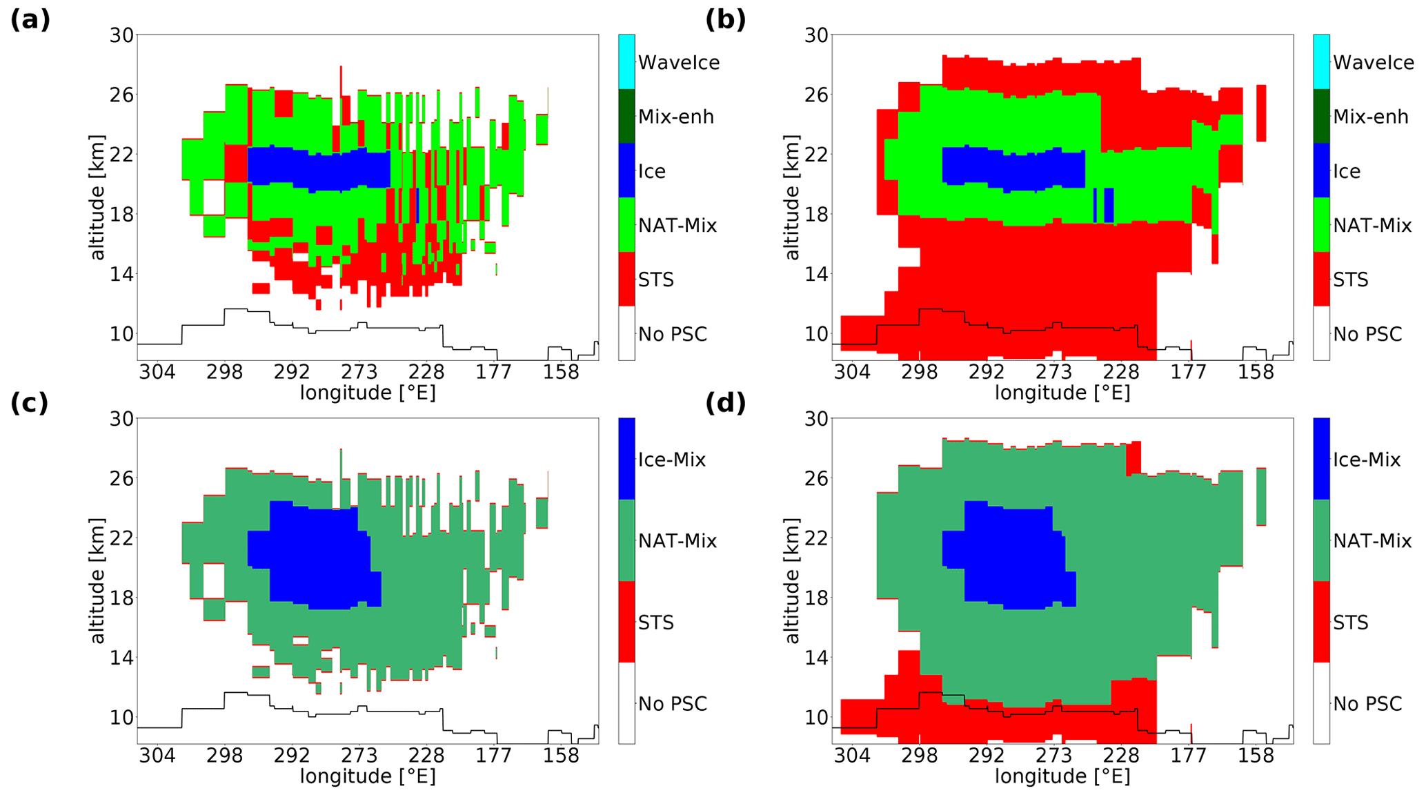
Figure A1 Composition of simulated PSCs along CALIPSO orbit 2 on 1 July 2007 according to the classification scheme from Pitts et al. (2018) after (a) and before (b) applying detection limits and instrument uncertainty. Panels (c) and (d) show the modeled PSC type (STS: STS occurrence only; NAT-Mix: NAT but no ice occurrence; Ice-Mix: ice occurrence).

Figure A2 Composite 2D histogram for July 2007, analogous to Fig. 1, for the simulation $S_{T,n\left(\mathrm{ice}\right),n(\mathrm{NAT},\max )}$.

Figure A3 As Fig. 4, but for the year 2006.

Figure A4 As Fig. 4, but for the year 2010.

Figure A5 As Fig. 5, but for the year 2006.

Figure A6 As Fig. 5, but for the year 2010.

Figure A7 Composite 2D histograms of CALIPSO measurements and SOCOL simulations as in Figs. 1, 6 and A2, but for the year 2006.

Figure A8 As Fig. A7, but for the year 2010.

Figure A9 As Fig. 7, but for the year 2006.

Figure A10 As Fig. 7 but for the year 2010.

Figure A11 As Fig. 8, but for the year 2006.

Figure A12 As Fig. 8, but for the year 2010.

Figure A13 As Fig. 9, but for the year 2006.

Figure A14 As Fig. 9, but for the year 2010.