High-resolution modeling of the distribution of surface air pollutants and their intercontinental transport by a global tropospheric atmospheric chemistry source–receptor model (GNAQPMS-SM)

Many efforts have been devoted to quantifying the impact of intercontinental transport on global air quality by using global chemical transport models with horizontal resolutions of hundreds of kilometers in recent decades. In this study, a global online air quality source–receptor model (GNAQPMS-SM) is designed to effectively compute the contributions of various regions to ambient pollutant concentrations. The newly developed model is able to quantify source–receptor (S-R) relationships in one simulation without introducing errors by nonlinear chemistry. We calculate the surface and planetary boundary layer (PBL) S-R relationships in 19 regions over the whole globe for ozone (O₃), black carbon (BC), and non-sea-salt sulfate (nss-sulfate) by conducting a high-resolution (0.5^∘ × 0.5^∘) simulation for the year 2018. The model exhibits a realistic capacity in reproducing the spatial distributions and seasonal variations of tropospheric O₃, carbon monoxide, and aerosols at global and regional scales – Europe (EUR), North America (NAM), and East Asia (EA). The correlation coefficient (R) and normalized mean bias (NMB) for seasonal O₃ at global background and urban–rural sites ranged from 0.49 to 0.87 and −2 % to 14.97 %, respectively. For aerosols, the R and NMB in EUR, NAM, and EA mostly exceed 0.6 and are within ±15 %. These statistical parameters based on this global simulation can match those of regional models in key regions. The simulated tropospheric nitrogen dioxide and aerosol optical depths are generally in agreement with satellite observations. The model overestimates ozone concentrations in the upper troposphere and stratosphere in the tropics, midlatitude, and polar regions of the Southern Hemisphere due to the use of a simplified stratospheric ozone scheme and/or biases in estimated stratosphere–troposphere exchange dynamics. We find that surface O₃ can travel a long distance and contributes a non-negligible fraction to downwind regions. Non-local source transport explains approximately 35 %–60 % of surface O₃ in EA, South Asia (SAS), EUR, and NAM. The O₃ exported from EUR can also be transported across the Arctic Ocean to the North Pacific and contributes nearly 5 %–7.5 % to the North Pacific. BC is directly linked to local emissions, and each BC source region mainly contributes to itself and surrounding regions. For nss-sulfate, contributions of long-range transport account for 15 %–30 % within the PBL in EA, SAS, EUR, and NAM. Our estimated international transport of BC and nss-sulfate is lower than that from the Hemispheric Transport of Air Pollution (HTAP) assessment report in 2010, but most surface O₃ results are within the range. This difference may be related to the different simulation years, emission inventories, vertical and horizontal resolutions, and S-R revealing methods. Additional emission sensitivity simulation shows a negative O₃ response in receptor region EA in January from EA. The difference between two methods in estimated S-R relationships of nss-sulfate and O₃ are mainly due to ignoring the nonlinearity of pollutants during chemical processes. The S-R relationship of aerosols within EA subcontinent is also assessed. The model that we developed creates a link between the scientific community and policymakers. Finally, the results are discussed in the context of future model development and analysis opportunities.

1 Introduction

For decades, under the influence of human activities, the concentrations of particulate matter, ozone, and their important precursors have greatly changed even in the most remote regions. Pollutants transported over long distances can have a negative impact on urban air quality, human health, and climate change (Fan et al., 2016). The hemispheric and intercontinental transport of air pollutants has always been an important international issue. For this reason, many countries and institutions around the world have launched a series of cooperative projects to study transboundary transportation, such as LRTAP (Long-range Transboundary Air Pollution), TRACE-A (Transport and Chemical Evolution over the Atlantic), LTP (Long-range Transboundary Air Pollutants in Northeast Asia), TRACE-P (Transport and Chemical Evolution over the Pacific; Carmichael et al., 2003), and TF HTAP (Task Force on Hemispheric Transport of Air Pollution). To better address and control global air pollution, it is vital to understand and quantify the sources of air pollutants from a global perspective.

Large-scale observation systems, including ground observations, aircraft, laser radars, and satellites, have been used to investigate the contributions from individual source regions to surface pollution (Venkatram and Karamchandani, 1986). Cooper et al. (2004) explained that air pollution can be transported across the North Pacific Ocean under the control of warm conveyor belts by using in situ measurements from an aircraft platform. Pal et al. (2020) used airborne in situ measurements of greenhouse gases (GHGs) to expound the important role of midlatitude cyclones in transporting GHGs across the eastern United States. An extensive dust event that originated in Africa and transported dust to South America was observed and tracked by CALIPSO lidar (Liu et al., 2008). However, because of the short duration of field observation activities and limited research area of observations, it is difficult to clarify the seasonal or interannual changes and attribute pollutants to specific source regions by only observation methods (Fiore et al., 2009). Recently, numerical global chemical transport models have been widely employed (Fiore et al., 2009) to quantify intercontinental source–receptor (S-R) relationships, as well as high-concentration pollution caused by local emissions. To a large extent, the quantitative assessment of intercontinental transport still depends on the model.

Many global chemical transport models have been used to study the distribution of air pollutants and estimate their intercontinental transport (Wai et al., 2016; Yang et al., 2017a). Sensitivity simulation, a numerical method, is widely used because of its relatively simple operation. It mainly refers to the reduction in emissions in the source region by a certain extent, such as 15 % or 20 %, or even directly returning to zero. Numerous studies have applied this method to assess S-R relationships, including black carbon (BC) transport to the Arctic (Sobhani et al., 2018, using a sulfur transport and deposition model (STEM)) and ozone transport among the Northern Hemisphere (Nopmongcol et al., 2017, using the Comprehensive Air Quality Model with Extensions (CAMx); X. Y. Li et al., 2014, using Model for Ozone and Related chemical Tracers, version 4 (MOZART-4); Y. Zhu et al., 2017, using the Goddard Earth Observing System model coupled to chemistry (GEOS-Chem)). These results all prove the hemispheric and intercontinental transport of air pollutants and highlight the importance of transboundary transport research from a broader perspective. However, sensitivity simulation methods usually ignore the nonlinearity of pollutants during chemical processes, which causes some errors in their estimated S-R relationships of secondary aerosols and O₃.

Sensitivity simulation also requires expensive computational resources, which results in most global simulations of pollutants running at coarse horizontal resolutions ranging from 1^∘ × 1^∘ to 5^∘ × 5^∘, such as 4^∘ × 5^∘ in J. Zhu et al. (2017), 2^∘ × 2.5^∘ in Han et al. (2020), 1^∘ × 1^∘ in Crippa et al. (2019), and 2.8^∘ × 2.8^∘ in Nagashima et al. (2017), and S-R relationships are limited to a few regions (e.g., Europe, North America, East Asia, South Asia). Many recent studies have revealed that horizontal resolution has a considerable influence on model performance in air quality simulations (Lin et al., 2010; Tao et al., 2020). Urban-scale pollution plumes are often unresolved in global model simulations with lower resolution, which tend to underestimate the magnitude of pollution formation and destruction, especially in urban areas (Huijnen et al., 2010). Consequently, the contribution of local emissions, especially from urban areas and regions with large coastlines, has been underestimated (Van Dingenen et al., 2018; Dentener et al., 2010; Fenech et al., 2018).

The tagged tracer method has proven to be a useful tool to investigate S-R relationships because of its better treatment of nonlinear chemistry and low computational cost (Nagashima et al., 2010; X. Y. Li et al., 2014). This method has already been implemented in CHASER (a chemical atmospheric general circulation model for study of atmospheric environment and radiative forcing) to calculate the relative contributions to surface ozone over Japan from a global perspective (Nagashima et al., 2010, 2017). Van Dingenen et al. (2018) developed a global reduced-form air quality source–receptor model based on a two-way nested global chemical transport model (Tracer Model version 5; TM5) and assessed the S-R relationships of 58 regions at a resolution of 6^∘ × 4^∘. Due to the limitation of computational efficiency or defects of models, many studies focus on a single species. Therefore, global high-resolution simulations of multiple air pollutants and their S-R relationships covering wider regions are needed and could play a key role in policy development (Amann et al., 2011).

In this study, by coupling an online S-R relationship module into the Global Nested Air Quality Prediction Modeling System (GNAQPMS), we developed a global tropospheric atmospheric chemistry source–receptor model (GNAQPMS-SM) and then conducted a 1-year high-resolution (0.5^∘ × 0.5^∘) simulation for 2018. Then, an extensive evaluation study was performed to assess the performance of the GNAQPMS with multiple platform observations. Using this module with GNAQPMS, we analyzed transport inside and outside East Asia in 19 regions over a global scale, allowing us to simultaneously identify the S-R relationships of O₃, PM_2.5, BC, and non-sea-salt sulfate (nss-sulfate).

This study is organized as follows: in Sect. 2, we introduce the model configurations, module descriptions, model domain, emission inventories, meteorological fields, and the observations and statistical parameters used in the evaluation. Section 3 presents the comparison of the model simulations with background observations, both at the surface and aloft. Model performance in three key regions is also displayed in Sect. 3. Section 4 illustrates the intercontinental transport of pollutants both in the surface layer and within the planetary boundary layer, and compares the results with the HTAP report and emission sensitivity simulation results. The discussions are summarized in Sect. 5.

2 Model description

GNAQPMS-SM includes two parts: GNAQPMS and an online source–receptor relationship module.

2.1 GNAQPMS

GNAQPMS is an offline global chemical transport model developed by the Institute of Atmospheric Physics, Chinese Academy of Sciences, and was briefly described by Wang et al. (2001), Li et al. (2008), and Chen et al. (2015). It includes horizontal and vertical advection (Walcek and Aleksic, 1998), diffusion (Byun and Dennis, 1995), detailed tropospheric O₃–NO_x–hydrocarbon gaseous (CBM-Z) chemistry (Zaveri and Peters, 1999), aqueous (RADM) chemistry (Stockwell et al., 1990), parameterization of dry and wet deposition (Zhang et al., 2003; Stockwell et al., 1990), heterogeneous chemistry (Li et al., 2012), and a unique dust particle deflation module (Wang et al., 2002). The horizontal resolution of the model is variable, and terrain-following coordinates are used vertically. Subgrid vertical transport of chemical species in GNAQPMS, including convection and boundary layer diffusion, are calculated by Emanuel's (1991) scheme and Byun and Dennis (1995) deriving from Global Weather Research and Forecasting (GWRF) model output variables, respectively. An aerosol thermodynamic model (ISORROPIAI1.7) is applied to compute the composition and phase state of the inorganic aerosol system in aerosol chemistry (Nenes et al., 1998). A hybrid volatility basis set (VBS) approach (Koo et al., 2014) is introduced to simulate organic aerosols (OAs), combining the simplicity of the 1-D VBS with the ability to represent the evolution of OAs in the 2-D space of oxidation state and volatility (Yang et al., 2019). The UV radiative transfer (TUV) model is coupled for the online calculation of 20 photolysis rates, including the aerosol, cloud, and gaseous species effects on photolysis (Li et al., 2011). A computationally efficient Mie algorithm-based scheme is adopted to calculate the single scattering albedo, Ångström coefficient, and aerosol optical depth online for input into the TUV model (Yu et al., 2012). Recently, a sectional microphysics aerosol model (APM, Yu and Luo, 2009) was coupled into GNAQPMS, and APM includes microphysics describing nucleation, condensation, coagulation, and thermodynamic equilibrium with local humidity in more detail (Chen et al., 2019). In APM, it is assumed that the aerosol mixing state is semi-external; that is, nucleated secondary particles are internally mixed, while primary particles, including BC, primary organic carbon, dust, and sea salt, are presumed to be made up of a seeding core and a secondary species coating. The coating of secondary species can change the hygroscopicity of aerosols and potentially influence their radiative and heterogeneous chemical effects. Both primary emitted particles and their coating species are traced in the model. GNAQPMS can reproduce physical and chemical processes in the atmosphere at both regional and global scales. It has been widely used to simulate the global distribution and international transport of mass and number concentrations of aerosol compositions, gaseous species (O₃ and CO), and mercury (Chen et al., 2015; Wang et al., 2017; Wei et al., 2019; Chen et al., 2019).

2.2 Online source–receptor relationship module

Air quality S-R models usually quantify the influence of air pollutant emissions in source regions, considering the impact of atmospheric physical and chemical processes (Van Dingenen et al., 2018). For primary pollutants (e.g., mineral dust, BC, and sea salt), only physical processes such as advection, diffusion, and dry and wet deposition can affect their S-R relationships. The response of their concentrations in receptor regions to emissions from source regions is nearly linear, so emission sensitivity analysis can provide an accurate S-R assessment. For secondary pollutants, the response of concentrations in receptor regions to source emissions is nonlinear because changes in emissions have the potential to influence the chemical formation of various secondary species. An air quality S-R model needs to include a nonlinear function relationship between source and receptor regions. Previous studies have suggested that the tagged tracer approach can prevent the introduction of nonlinear errors during chemical processes and is suitable for evaluating the contributions of different source regions to secondary pollutants (Derwent et al., 2004; Li et al., 2013). In this study, an online source–receptor relationship module based on a tagged tracer approach is coupled into GNAQPMS. In this module, we assume that each tagged pollutant at each grid from different source regions (C^T) shares the same loss velocities with total pollutants in the host model (e.g., dry and wet depositions, outflow by advection, convection, and diffusion). Therefore, the fraction of each tagged pollutant in total concentrations ($F_{{\mathrm{C}}^{\mathrm{T}}}$) at a given grid cell is not changed by the removal processes. Primary pollutants are tagged by the geographical emitting locations, and $F_{{\mathrm{C}}^{\mathrm{T}}}$ is calculated by Eq. (1):

$$\begin{array}{}\text{(1)}& {\left({\displaystyle \frac{\mathrm{d}{F}_{{\mathrm{C}}^{\mathrm{T}}}}{\mathrm{d}t}}\right)}_{ij}=\left(E_{ij}+{\left(M_{ij}\right)}_{\mathrm{dif}+\mathrm{adv}+\mathrm{conv}}\right)/C,\end{array}$$

where i represents the ith geographical source region and j represents the jth grid cell. C^T is the mass concentration of tagged pollutant from the ith source region. $F_{{\mathrm{C}}^{\mathrm{T}}}$ is the fraction of tagged species from the ith region in the total mass concentration of this tagged species at the jth grid cell. E_ij is the pollutants emitted from the ith source region at the jth grid cell; hence, when the jth grid is outside region i, E_ij is equal to zero. M_ij is the C^T inflows from the neighboring grid cells caused by advection, diffusion and convection and is computed by the inflow fluxes and the ith C^T fraction of those neighboring grid cells. C is the total mass concentration of tagged species. It is obvious that the contribution of each source region to the receptor region is strictly positive. The sum of all relative contributions from individual sources in the receptor region equals 100 %, and the sum of absolute contributions is equal to the total concentrations for each species.

Different from primary pollutants, secondary species are formed through hundreds and thousands of reactions. $F_{{\mathrm{C}}^{\mathrm{T}}}$ is calculated by Eq. (2).

$$\begin{array}{}\text{(2)}& {\left({\displaystyle \frac{\mathrm{d}{F}_{{\mathrm{C}}^{\mathrm{T}}}}{\mathrm{d}t}}\right)}_{ij}=\left(P_{ij}+{\left(M_{ij}\right)}_{\mathrm{dif}+\mathrm{adv}+\mathrm{conv}}\right)/C\end{array}$$

For ozone, O₃ is tagged by the geographical location where it was produced in this module, as shown in Eq. (2). P_ij is the gross production of the ith source region at the jth grid cell and is calculated by

$$\begin{array}{}\text{(3)}& \begin{array}{rl}{P}_{ij}& =\left\{\begin{array}{l}{P}_{{\mathrm{O}}_{\mathrm{3}}},\text{the}j\text{th}\text{grid is within}i\text{th region}\\ \mathrm{0},\text{the}j\text{th grid is outside}i\text{th region}\end{array}\right.\\ P& =k_{\mathrm{1}}\left[{\mathrm{HO}}_{\mathrm{2}}\right]\left[\mathrm{NO}\right]+k_{\mathrm{2}}\left[{\mathrm{RO}}_{\mathrm{2}}\right]\left[\mathrm{NO}\right],\end{array}\end{array}$$

k₁ and k₂ are the rate coefficients of HO₂+NO and RO₂+NO, respectively. This method mainly focuses on the direct transport of ozone itself, while the photochemical production of precursors from source regions during transport (indirect transport) is considered to be the contribution from ozone production regions. Similar methods were employed to evaluate the long-distance transport of O₃ by Sudo and Akimoto (2007).

For secondary aerosols, all components are directly related to specific precursor species. We assume that all species have the same reactive properties in each given region, period and emission type (e.g., power plant emissions have the same response to transportation emissions). The P_ij for irreversibly partitioning species such as sulfate is apportioned to the primary precursor SO₂ as follows:

$$\begin{array}{}\text{(4)}& P_{{{\mathrm{SO}}_{\mathrm{4}}}_{ij}}=\mathrm{\Delta }{\mathrm{SO}}_{\mathrm{4}}\times {\displaystyle \frac{C_{{{\mathrm{SO}}_{\mathrm{2}}}_{ij}}^{\mathrm{T}}}{C_{{{\mathrm{SO}}_{\mathrm{2}}}_j}}}.\end{array}$$

ΔSO₄ is the change in total mass concentration after chemical transformation. $C_{{{\mathrm{SO}}_{\mathrm{2}}}_{ij}}^{\mathrm{T}}$ and $C_{{{\mathrm{SO}}_{\mathrm{2}}}_j}$ represent the concentrations of the ith tagged source and total SO₂ in the jth grid, respectively. For reversibly partitioning species such as nitrate, ammonium, and semivolatile secondary organic aerosols, the chemical equilibrium for aerosols and their gaseous precursors from each source category (i) is set equal to the equilibrium for the total species concentrations. The P_ij for the aerosol phase is described in Eq. (5). More details on aerosols can be found in Wagstrom et al. (2008) and Wu et al. (2017).

$$\begin{array}{}\text{(5)}& \begin{array}{rl}{P}_{{\mathrm{aerosol}}_{ij}}=& \left(C_{{\mathrm{aerosl}}_{ij}}^{\mathrm{T}}+C_{{\mathrm{precursor}}_{ij}}^{\mathrm{T}}\right)\\ & \times {\displaystyle \frac{C_{{\mathrm{aerosol}}_j}}{C_{{\mathrm{aerosol}}_j+C_{{\mathrm{precursor}}_j}}}}-C_{{\mathrm{aerosl}}_{ij}}^{\mathrm{T}}\end{array}\end{array}$$

This online S-R module has been successfully applied in regional studies to estimate the impact of transboundary transport on aerosols and ozone in East Asia in both long-term (Li et al., 2008; Y. Li et al., 2014a, 2016) and heavy episodes (Wu et al., 2011, 2017). Recently, it has been coupled to a routine air quality forecast model in China and has demonstrated its key role in policy development. These applications give some confidence in simulating the global S-R relationships of pollutants.

2.3 Model domain

To clearly identify different sources of pollutants and quantify the influences of different regions, we separate the global domain into 19 regions, as illustrated in Fig. 1a. Asia is separated into four regions (i.e., South Asia, Southeast Asia, central Asia, and East Asia). To better analyze the S-R relationships inside and outside East Asia (EA), EA is further divided into four regions: Japan, the Republic of Korea, North Korea, and China. The United States and Canada are merged into one region, North America (NAM). Greenland is included in Europe. The ocean is separated into two regions: the ocean north of 66.5^∘ N and the rest of the ocean. The definitions of 19 source regions are listed in Table S1 in the Supplement. In particular, to reduce the error in calculating the contribution of coastal activities to marine emissions, we extend the land boundary outward by the distance of four grid cells.

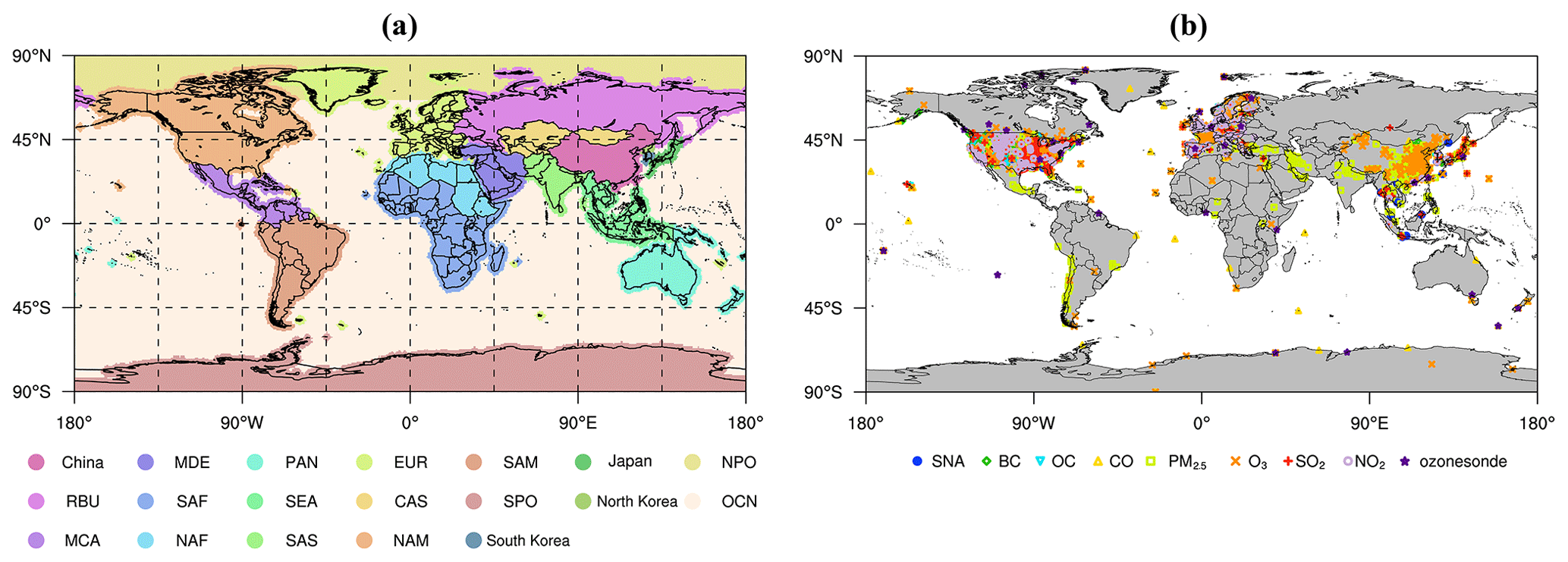
Figure 1 (a) Model domain and (b) stations for the evaluation used in this study.

Simulation is performed for 2018 after an initial model spin-up of 6 months, with a horizontal resolution of 0.5^∘ × 0.5^∘. A total of 20 vertical layers are divided in this study. The bottom layer is approximately 50 m, and the top layer is approximately 20 km. After calculation of tropospheric height, the monthly stratospheric ozone above the troposphere is taken from the climatic mean output from MOZART v2.4 (Horowitz et al., 2003; Logan, 1999). The model outputs concentrations of air pollutants once an hour.

2.4 Emission inventory

The global anthropogenic emissions of air pollutants except NH₃ and non-methane volatile organic compound (NMVOC) emissions are derived from the Emissions Database for Global Atmospheric Research (EDGAR v5.0; Crippa et al., 2020; data available at https://edgar.jrc.ec.europa.eu/overview.php?v=50_AP, last access: 28 July 2020) based on 2015 with a resolution of 0.1^∘ × 0.1^∘, while NMVOC is from EDGAR v4.3.2. NH₃ is adopted from the HTAP v2.2 emissions inventory for 2010 (Janssens-Maenhout et al., 2015; data available at https://edgar.jrc.ec.europa.eu/htap_v2/index.php?SECURE=123, last access: 28 July 2020) because the NH₃ emissions in China from the HTAP v2.2 inventory are more consistent with those from Chinese regional inventories compared with EDGAR v5.0. Anthropogenic emissions are mainly divided into five source categories: residential, agricultural, transportation, industrial, and power sources. The biogenic emissions of CO, isoprene, methanol, pinene, and other monoterpenes are provided by the Model of Emissions of Gases and Aerosols from Nature (MEGANv2.1; Guenther et al., 2012) developed by the National Center for Atmospheric Research (NCAR). Emissions from biomass burning are calculated from the Fire Inventory from NCAR (FINN v1) emissions from Wiedinmyer et al. (2011). FINN provides daily global emissions with a resolution of 0.1^∘ × 0.1^∘ in 2018 based on satellite observations for detecting active fires as thermal anomalies and land cover change (Wiedinmyer et al., 2011). Gas flaring emissions ECLIPSE V5a (Klimont et al., 2017; https://iiasa.ac.at/web/home/research/researchPrograms/air/ECLIPSEv5a.html, last access: 28 July 2020) are added in the inventory, and this will be mentioned later. Climatic 1^∘ × 1^∘ lightning emissions of nitric oxide from the Global Emissions Inventory Activity (GEIA) database are applied in this study (Price et al., 1997). Soil NO_x emissions are from global hourly emissions for soil NO_x (Hudman et al., 2012; data available at http://ftp.as.harvard.edu/gcgrid/data/ExtData/HEMCO/OFFLINE_SOILNOX/v2019-01/, last access: 28 July 2020). Volcanic SO₂ emissions are from Carn et al. (2015) (data available at http://ftp.as.harvard.edu/gcgrid/data/ExtData/HEMCO/VOLCANO/v2019-08/, last access: 28 July 2020). CO, dimethylsulfide (DMS), CHBr₃, CH₃I, CH₂Br₂, and carbonyl sulfide (OCS) from the oceans are taken from the CAMS-81 project with a resolution of 0.5^∘ (Granier et al., 2019). Table 1 summarizes the total emissions of anthropogenic and natural sources from several regions used in this study. These results show similar emission magnitudes to those in previous global emission inventories (Badia et al., 2017; Yang et al., 2017a; Klimont et al., 2017).

Table 1 Total emissions from several regions used in the GNAQPMS simulation (Tg/yr).

2.5 Meteorological fields

The GWRF version 3.6 model was used to generate essential input meteorological data for GNAQPMS. GWRF is an extension of the mesoscale Weather Research and Forecasting (WRF) model and was developed for global weather research and forecasting applications (Y. Zhang et al., 2012). Compared to traditional general circulation models (GCMs), GWRF enables a unified framework for the modeling of atmospheric processes and their interactions across scales spanning from global to local scales through one-way or two-way nesting. In this study, the GWRF model is driven by National Centers for Environmental Prediction (NCEP) Final Analysis (FNL) data. The global horizontal spatial resolution is 0.5^∘ × 0.5^∘. Vertically, the GWRF data require interpolation for input into GNAQPMS. The comparison between simulated meteorological fields and reanalysis data is shown in Fig. S1 in the Supplement. GWRF can simulate the spatial distribution of wind speed well, with deviations of less than 1 m/s in most regions. Compared with Global Precipitation Climatology Project (GPCP) reanalysis data, the simulated precipitation field may be underestimated by approximately 30 %, which is similar to previous results (Sugiura et al., 2006; Mori et al., 2020).

2.6 Observation data and statistical parameters

The ground sites used for comparison are shown in Fig. 1b. Observations for CO are collected from the World Data Center for Greenhouse Gas (WDCGG; data available at https://gaw.kishou.go.jp/search, last access: 28 July 2020). The measurement data for O₃ in Europe are obtained from the European Monitoring and Evaluation Programme (EMEP; data available at http://ebas.nilu.no/, last access: 16 June 2020), those in the US are from the United States Environmental Protection Agency (EPA; data available at https://aqs.epa.gov/aqsweb/airdata/download_files.html, last access: 3 August 2020), and those in East Asia are from the Acid Deposition Monitoring Network in East Asia (EANET; data available at https://www.eanet.asia/, last access: 3 August 2020) and the Chinese National Environment Monitoring Center (CNEMC; data available at http://www.cnemc.cn/, last access: 3 August 2020). The vertical observation data of O₃ come from the World Ozone and Ultraviolet Radiation Data Centre (WOUDC; data available at https://www.woudc.org/home.php, last access: 3 August 2020). The observation data for PM_2.5 and PM_2.5 components in different regions are collected from IQAir (data available at https://www.iqair.cn/cn-en/world-air-quality-report, last access: 3 August 2020), CNEMC, EANET, EMEP, and the United States Interagency Monitoring of Protected Visual Environment (IMPROVE; data available at http://views.cira.colostate.edu/fed/QueryWizard/Default.aspx, last access: 3 August 2020). The SO₂ observations are collected from EANET, EPA, and EMEP. NO₂ columns are compared with tropospheric NO₂ column concentration data from the Tropospheric Monitoring Instrument (TROPOMI; van Geffen et al. (2020); data available at http://www.temis.nl/airpollution/no2.php, last access: 3 October 2020), and the resolution of monthly TROPOMI NO₂ data from the Royal Netherlands Meteorological Research Institute (KNMI) used in our paper is 0.125^∘ × 0.125^∘. The aerosol optical depth (AOD) from the level-3 atmosphere monthly global product (MOD08_M3; Platnick, 2015; data available at https://ladsweb.modaps.eosdis.nasa.gov/archive/allData/61/MOD08_M3/, last access: 3 October 2020), retrieved from MODIS Terra, is used to evaluate the simulated AOD and the horizontal resolution is 1^∘ × 1^∘. We compared the spatial distribution of AOD and NO₂ columns through one-by-one correspondence between the simulation time and the MODIS, TROPOMI observed time, the model grid cell and MODIS, TROPOMI data grid cell. Note that the concentration of PM_2.5 mentioned below refers to the total concentration of sulfate, nitrate, ammonium, primary PM_2.5, organic mass (OM), BC, dust, and sea salt. We multiplied all organic carbon (OC) values by a conversion factor of 1.8 to obtain OM, and SNA (mentioned below) refers to the sum of sulfate, nitrate, and ammonium.

If observations in the above datasets are available in 2018, the observation data in 2018 are used. If not, the multiyear observation average is used. When focusing on seasonal variations, the year is divided into four seasons: March–April–May (MAM), June–July–August (JJA), September–October–November (SON), and December–January–February (DJF). The statistical parameters used in the evaluation include FAC2, the correlation coefficient (R), and the normalized mean bias (NMB). FAC2 refers to the proportion of the simulated results falling between 0.5 and 2 times the observed results, and the formulas for R and NMB are as follows:

$$\begin{array}{}\text{(6)}& {\displaystyle }R={\displaystyle \frac{{\sum }_{i=\mathrm{1}}^n\left({\mathrm{sim}}_i-\stackrel{\mathrm{‾}}{\mathrm{sim}}\right)\left({\mathrm{obs}}_i-\stackrel{\mathrm{‾}}{\mathrm{obs}}\right)}{\sqrt{\sum _{i=\mathrm{1}}^n{\left({\mathrm{sim}}_i-\stackrel{\mathrm{‾}}{\mathrm{sim}}\right)}^{\mathrm{2}}}\sqrt{\sum _{i=\mathrm{1}}^n{\left({\mathrm{obs}}_i-\stackrel{\mathrm{‾}}{\mathrm{obs}}\right)}^{\mathrm{2}}}}}\text{(7)}& {\displaystyle }\text{NMB}={\displaystyle \frac{{\sum }_{i=\mathrm{1}}^n\left({\mathrm{sim}}_i-{\mathrm{obs}}_i\right)}{{\sum }_{i=\mathrm{1}}^n{\mathrm{obs}}_i}},\end{array}$$

where sim_i and $\stackrel{\mathrm{‾}}{\mathrm{sim}}$ are the simulation results of the ith station and the average of the simulations of all stations, respectively, and obs_i and $\stackrel{\mathrm{‾}}{\mathrm{obs}}$ are the observation value of the ith station and the average of the observations of all stations, respectively.

3 Global distribution and evaluation

Detailed evaluation of GNAQPMS annual and seasonal results with observations is central for assessing the ability of GNAQPMS to study S-R relationships. In this section, we compare the measured and simulated seasonal or annual concentrations of surface ozone, CO, PM_2.5, and its components.

3.1 Model evaluation against background concentrations

To investigate the model performance in background stations, we selected more than 60 stations all over the world from WDCGG.

3.1.1 O₃

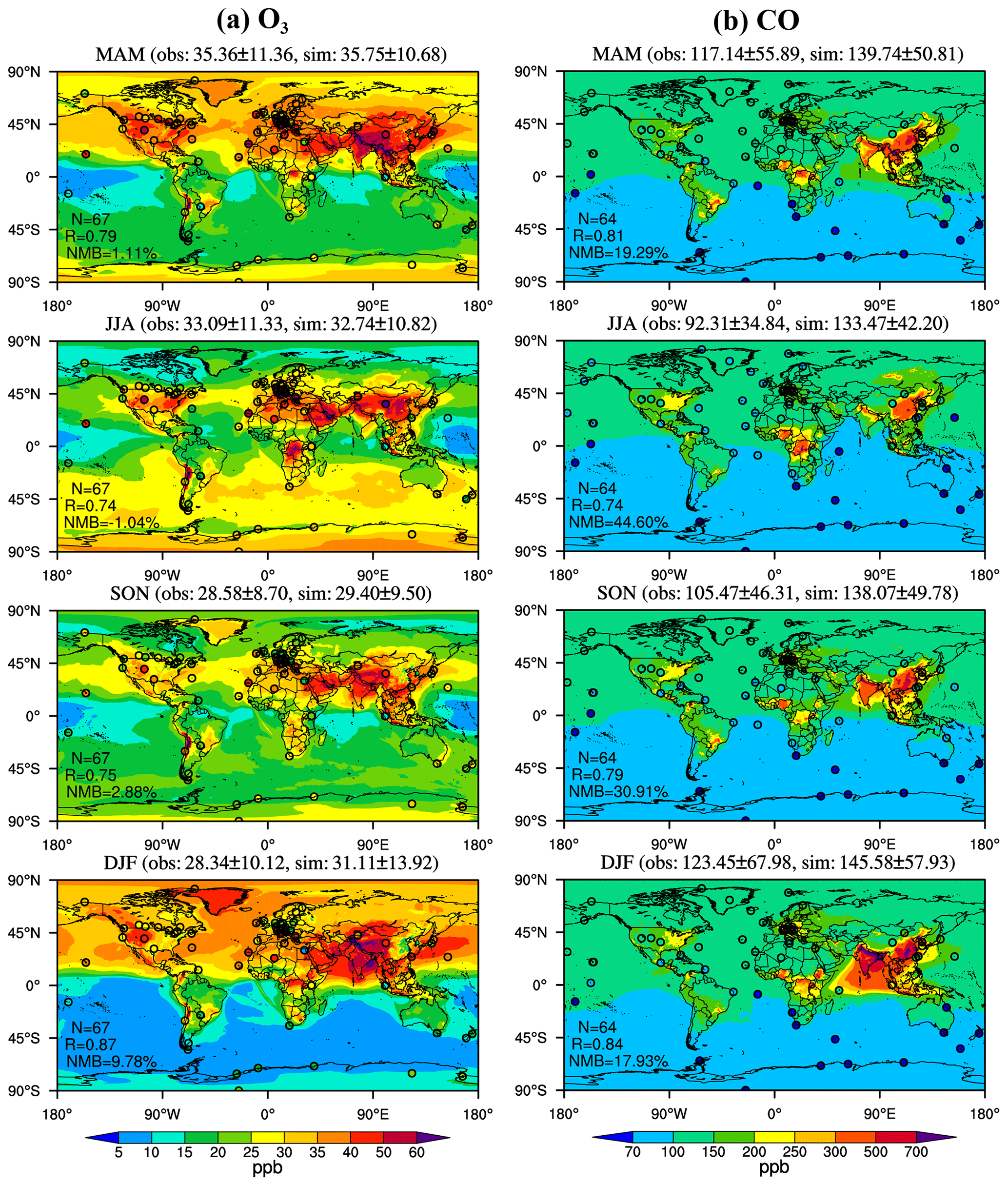
Figure 2 Spatial distributions of simulated (shaded) surface (a) O₃ and (b) CO concentrations compared with WDCGG observations (solid circles).

Figure 2a shows a snapshot of the simulated seasonal surface O₃ concentration against WDCGG observations at background stations from a global perspective in 2018. In general, the observed magnitudes and seasonal variations of O₃ are reasonably reproduced by the model, with R values of 0.74–0.87 and NMBs of −1 %–10 % in the four seasons (N=67). The model performance is similar to the BCC-GEOS-Chem (an online global atmospheric model, by coupling the GEOS-Chem chemical transport model as an atmospheric chemistry component in the Beijing Climate Center atmospheric general circulation model) performance reported by Lu et al. (2020). Among the four seasons, the model shows the lowest model biases of −0.35–0.39 ppb relative to WOUDC surface observations in MAM and JJA. In MAM, the model captured a band of high O₃ with values of 30 ppb or higher in most Northern Hemisphere and southern polar regions. The highest values reached 40–60 ppb, extending from north Africa to East and South Asia. In JJA, this simulated high ozone band in the Northern Hemisphere was focused over northern midlatitude (30–45^∘ N) continents as a result of intensive photochemical production involving anthropogenic NO_x and VOC_s. Interestingly, O₃ mixing ratios in the Southern Hemisphere significantly increase to 35–40 ppb due to the injection of stratospheric O₃, which is consistent with observations, as shown in Fig. S2. The model tends to overestimate tropospheric ozone levels in DJF, with an NMB of 9.78 %. This overestimation is more prominent in the northern high latitudes because of the overestimation of the stratosphere to troposphere in this model, as will be discussed later.

Simulated vertical profiles of ozone are compared with ozonesonde observations in six regions from WOUDC in Fig. 3. The simulated magnitude and vertical gradient of ozone are generally in good agreement with observations throughout the depth of the middle–lower troposphere (surface-500 hPa). Model results and observations generally fell within 1 standard deviation of each other. In EUR and NAM, the simulation also accurately characterizes the vertical variation in O₃ in the whole troposphere. However, the simulation overestimated O₃ mixing ratios in the upper troposphere and stratosphere (500–200 hPa) in other regions. This is likely caused by the simplified treatment of the stratosphere to the troposphere in our model. In the model, stratospheric O₃ is constrained by relaxation towards zonally and monthly averaged values from ozone climatologies from Logan (1999) and Horowitz et al. (2003). These monthly values may cause the model to produce virtual stratosphere to troposphere events that are not observed by low-frequency ozonesonde in WOUDC (only one sample every 1–2 weeks). The coarse vertical resolution in the upper troposphere and stratosphere introduces errors in the modeling dynamics of ozone exchange between the stratosphere and the troposphere. Similar phenomena have also been reported in previous studies (Horowitz et al., 2003; Miyazaki et al., 2020; Verstraeten et al., 2013), which reported that representations of the stratosphere–troposphere exchange in four models caused a large overestimation of ozone at 500–90 hPa.

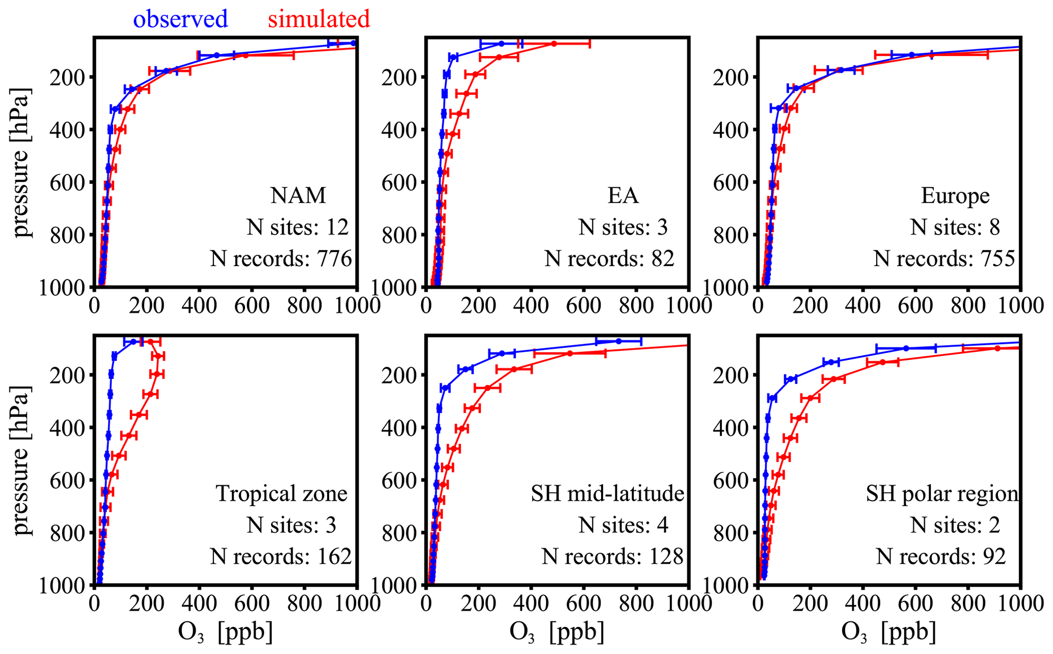
Figure 3 Comparisons of GNAQPMS-simulated annual mean ozone vertical profiles with ozonesonde observations averaged over some regions. Horizontal blue and red bars are the standard deviations of observations and simulations, respectively.

3.1.2 Carbon monoxide (CO)

The annual mean concentration of CO simulated by GNAQPMS compared with WDCGG observations is shown in Fig. 2b. CO concentrations are well correlated with observations, with R values of 0.74–0.84 year round (N=64), while simulated concentrations are slightly higher, with NMBs ranging from 17.93 % to 44.60 %. The lowest model biases compared to surface observations are 22.13–22.6 ppb in DJF and MAM. The seasonal variation in CO is not obvious in the ocean, while it is significant on the continents. High values are always found in the regions with significant emissions from industrial sources, such as the US, Europe, South Asia (SAS), and EA these fossil fuel combustion regions, and in those with significant emissions from biomass burning, such as central Africa, South America, and Southeast Asia (SEA), in all four seasons. The seasonal results show that the CO concentration over EA and SAS peaks during DJF, followed by MAM and SON, since there is more fossil fuel combustion for heating, whereas central Africa experiences a maximum in JJA, which is mainly due to the stronger biomass burning and biogenic emissions. The positive biases in JJA reach 41.16 ppb, which is in part due to the lower OH levels and higher CO direct emission. The anthropogenic emission of CO in this study is 686.7 Tg/yr, which is higher than values in other studies, e.g., Horowitz et al. (2020) used 612.4 Tg/yr for year 2014. The main sink of CO is by reaction with OH. The tropospheric mean concentration of OH in our model is 11.9×10⁵ molecules/cm³, which is in good agreement with previous studies, e.g., Badia et al. (2017) with 11.5×10⁵ molecules/cm³ and Voulgarakis et al. (2013) with 11.1 ± 1.8 ×10⁵ molecules/cm³ from 14 models for 2000. Therefore, the overestimation of CO is mainly due to high CO anthropogenic emissions.

3.1.3 Nitrogen dioxide (NO₂)

Tropospheric NO₂ columns from TROPOMI data are compared with GNAQPMS in Fig. 4. As shown in Fig. 4, the column concentration of NO₂ has a range of 0.4-15×10¹⁵ molecules/cm² over most of the land, the magnitude of which is well reproduced. Because of the short lifetime of NO_x, tropospheric NO₂ columns are considered to be closely sensitive to land surface NO_x emissions. As shown in Fig. 4a, the anthropogenic source areas of EA, Europe, and the eastern US are the major NO_x emission sources, with high values in SON and DJF. The model satisfactorily captures seasonality and high-value regions of NO₂ columns in the vertical troposphere. The largest differences are found for eastern China, where GNAQPMS reaches levels of 15 ×10¹⁵ molecules/cm², whereas observations are on average 10 ×10¹⁵ molecules/cm². This overestimation is likely because China implemented the toughest-ever clean air policy in 2013–2017 and reduced NO_x emissions by 7.95 Tg (Zhang et al., 2019). This is not reflected by the EDGAR v5.0 emission inventory. A negative bias for TROPOMI data compared to the ground-based measurements (Verhoelst et al., 2021) may also be a reason for our model positive biases.

Figure 4 Spatial distributions of seasonal mean NO₂ columns from (a) GNAQPMS averaged in 2018 and (b) the TROPOMI data.

3.1.4 PM_2.5 and aerosol optical depth

Figure 5c displays the seasonal variation in PM_2.5. The concentrations over the continents are higher than those over the ocean in most regions, and the simulated PM_2.5 is less than 1 µg/m³ in the northern and southern polar regions, as shown in Fig. 5c. There is a high PM_2.5 band with values of approximately 10 µg/m³ in the southern midlatitudes, which is mainly caused by sea salt. The major PM_2.5 hotspots are over India, East Asia, and central Africa, and PM_2.5 reaches a peak during DJF, followed by lower values during MAM, and the lowest values are during JJA and SON since there is higher biomass and fossil fuel burning for heating, less precipitation, and strengthened positive feedback between aerosols and the planetary boundary layer (PBL) (Petaja et al., 2016) during DJF. AOD, which is the total column aerosol extinction, is positively correlated with the total aerosol mass concentration in an atmospheric column. We compare the annual AOD with MODIS satellite data in Fig. 5a–b. The AOD over the ocean ranges from 0.1 to 0.3, which is mainly related to sea salt. The high AOD regions are central and west Africa and South and East Asia, and AOD reaches a maximum in JJA and connects into a high band at midlatitudes in the Northern Hemisphere. The maximum in central Africa and west Africa in Fig. 5a is due to the tremendous amount of carbonaceous aerosol emitted by biomass burning, which often takes place in JJA. The model reproduces this distribution well, although there is a slightly negative bias in high-value regions, especially in JJA. The high AOD in South and East Asia related to high anthropogenic emissions is underestimated. The major hotspots of AOD are consistent with those of PM_2.5. GNAQPMS shows a weaker AOD in most regions, which may be related to the low PM_2.5 in the simulation, as will be discussed later, and may be due in part to uncertainty in satellite AOD datasets (Li et al., 2009).

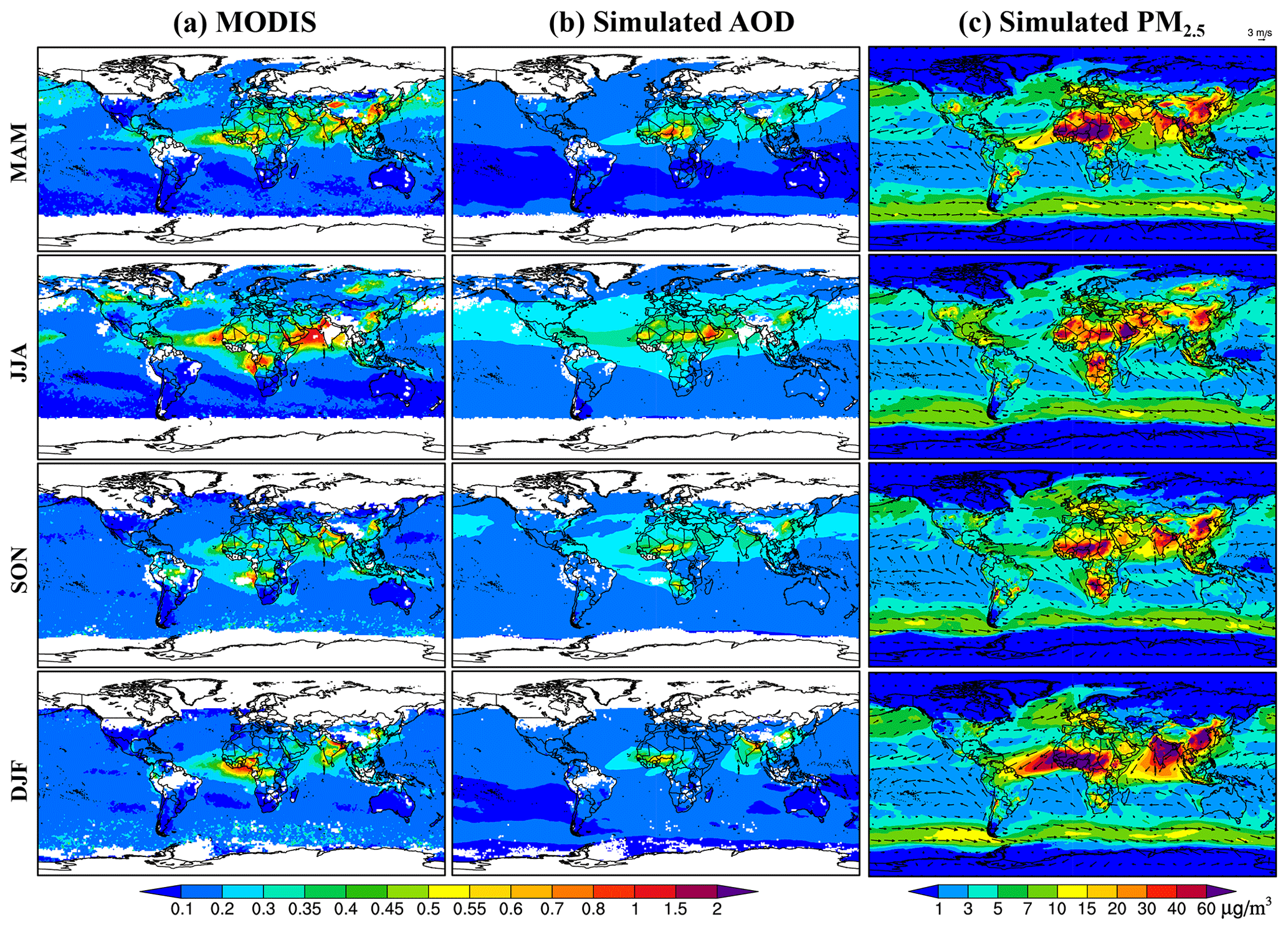
Figure 5 Spatial distributions of seasonal mean AOD at 550 nm from (a) MODIS data and (b) GNAQPMS averaged in 2018 and (c) PM_2.5 in GNAQPMS.

3.2 Model evaluation against regional/urban concentrations

O₃ and other secondary pollutants significantly vary in regions with large gradients in emissions of NO_x and other precursor emissions. This requires a model with sufficient spatial and temporal resolution, and coarse grids usually do not adequately capture urban-scale pollutant levels and gradients when the urban area occupies only a fraction of the grid cell (Huijnen et al., 2010). In this study, GNAQPMS employs a fine resolution of 0.5^∘ × 0.5^∘ and outputs hourly data, which provides us with a good opportunity to investigate detailed air pollutant distributions and their origins in key regions from a global perspective. Here, we evaluate surface O₃, PM_2.5, and its compositions in East Asia, Europe, and North America from the CNEMC, EANET, EMEP, and IMPROVE air quality networks.

Figure 6 Scatterplots of simulated (sim) and observed (obs) annual mean concentrations. The black dotted lines are the 2:1, 1:1, and 1:2 reference lines from left to right. Different regions are plotted with circles in different colors.

Figure 6 shows a comparison of the annual surface mean simulated O₃, NO₂, PM_2.5, and PM_2.5 components and SO₂ concentrations with ground-based observations in different regions, and detailed information on R and NMB is provided in Table S2. As shown in Fig. 6a, surface O₃ shows remarkable agreement with the observations. The annual average simulated O₃ concentration of all stations worldwide is 33.38 ppb, while the mean of the observed data is 32.23 ppb, with an NMB of 3.55 % and an FAC2 of 99.78 %. For NO₂, GNAQPMS shows high correlations with observations and no significant annual biases in EA, EUR, and NAM. The simulated and observed NO₂ values are 3.57 and 4.36 ppb, respectively, and 69.14 % of stations are within a factor of 2 of observations, with R values of 0.89, 0.87, and 0.56 and NMBs of −25.69 %, −31.15 %, and 2.49 % for EA, EUR, and NAM, respectively (see Fig. 6b and Table S2). NO₂ has a short lifetime and is greatly affected by local sources, and the model shows stronger spatial correlations with observations than previous studies in East Asia (Li et al., 2012) and Europe (Mar et al., 2016; Karamchandani et al., 2017). In addition, the annual average NMB of −18.21 % with respect to NO₂ is also in line with previously published studies (Zhang et al., 2013).

In Fig. 6c, the modeled PM_2.5 is 18.48 µg/m³, while the mean of the measured data is 23.27 µg/m³, with an NMB of −20.56 % and an FAC2 of 86.57 %. Simulated versus observed PM_2.5 concentrations across 417 stations highlight the underprediction of PM_2.5. Due to the large contribution of biomass burning and fossil fuel combustion, PM_2.5 is higher in China and SEA than in EUR and NAM, as shown in Fig. 6c. The concentration in SAM is obviously underestimated, which may be related to the uncertainty of the emission inventory in SAM. At present, most models generally underestimate the concentration of BC (Shindell et al., 2008), and the difficulties of BC simulation are the parameterization scheme selection of BC aging and wet scavenging processes, as well as the lack of BC emission sources. According to a previous study, adding gas flaring emissions can improve the surface BC concentration biases, especially in the Arctic (Huang et al., 2015); therefore, we add the ECLIPSE V5a flaring emissions in the inventory. However, the simulated concentration of BC is 186.27 ng/m³, which is underestimated by approximately 174 ng/m³, with an NMB of −48.37 %, while the R value is up to 0.9 (Fig. 6d). Only approximately 44 % of stations are within a factor of 2 of observations. NMB values are −52.08 %, −20.30 %, and −49.97 % over EA, EUR, and NAM, respectively. The performance for Europe is in agreement with BC simulations using GEOS-Chem in Europe, showing that BC concentrations are underpredicted by approximately 30 % (Huang et al., 2015; Wang et al., 2014), whereas the performance for EA and NAM is unsatisfactory. Similar to BC, the model can accurately capture the observed spatial distribution (R=0.82) but underestimates the levels of OM, with NMB and FAC2 values of −49.33 % and 46.3 %, respectively (Fig. 6e). This underestimation of BC and OM is more severe over NAM. However, the spatial correlation of BC and OM is better than the result in Carter et al. (2020). In Fig. 6f, simulated SNA shows better agreement with observations than carbonaceous aerosols. The simulated and observed values are 2.76 and 3.42 µg/m³, respectively, and 77.12 % of stations are within a factor of 2 of observations. GNAQPMS tends to underestimate the concentration of sulfate, with an NMB value of −39.14 % (Fig. 6g). Compared with an NMB of −1.53 % in EA in Uno et al. (2017) and an NMB of −3.9 % from GEOS-Chem results in the US in L. Zhang et al. (2012), our performance of sulfate needs to be improved. This negative bias could also be attributed to ignoring subgrid aerosol variations in the model (Qian et al., 2010; Yang et al., 2017a) and heterogeneous chemistry on aerosol surfaces (Bauer and Koch, 2005; Andreae and Crutzen, 1997) and could still be related to the positive bias of SO₂ with an NMB of 44.91 %, as shown in Fig. 6h. Partial incomplete oxidation and a low rate of conversion from SO₂ gas to sulfate particles in GNAQPMS could lead to the high concentration of SO₂ and low concentration of sulfate in the atmosphere. Generally, GNAQPMS has a good capability of reproducing the magnitudes of pollutants in regions.

3.2.1 East Asia

In Fig. 7, the observations from CNEMC and EANET are used. GNAQPMS captures the surface O₃ seasonal variation in eastern and western China. Year-round O₃ concentrations averaged over eastern China are approximately 20 ppb lower than those over western China. Surface O₃ over southwest China reaches a maximum in DJF and MAM and a minimum in JJA and SON, whereas that over eastern China reaches a peak in JJA and a trough in DJF, and this seasonality is determined by abundant photochemical reactions in JJA and the East Asian monsoon. The enhanced titration of O₃ with the increase of NO_x in DJF could also be a possible reason. The model also captures the high values during MAM in Japan. The peak in the western Pacific is consistent with the high values in Japan. Figure 7b shows scatterplots of simulated and observed seasonal surface concentrations of O₃. As shown in Fig. 7b, the O₃ simulations at most sites are within a factor of 2 of observations, with R ranging from 0.67 to 0.86 and NMB ranging from −1.26 % to 7.81 % in different seasons. The observed seasonal mean O₃ concentration in EA is between 21.37 and 42.46 ppb, while the simulated concentration is between 23.04 and 44.07 ppb. The simulation annual and seasonal results of O₃ in EA match those of regional models participating in the Model Inter-Comparison Study for Asia Phase III (MICS-Asia III) (Li et al., 2019). Figure 7c shows the frequency of O₃ NMB values, distributed as a function of NMB. NMB of O₃ in MAM is most frequently between −15 % and −10 % in EA, and the frequency of occurrence of lower O₃ NMB values dramatically decreases. The NMBs in the other three seasons are most frequently within ±5 % and show an approximately normal distribution.

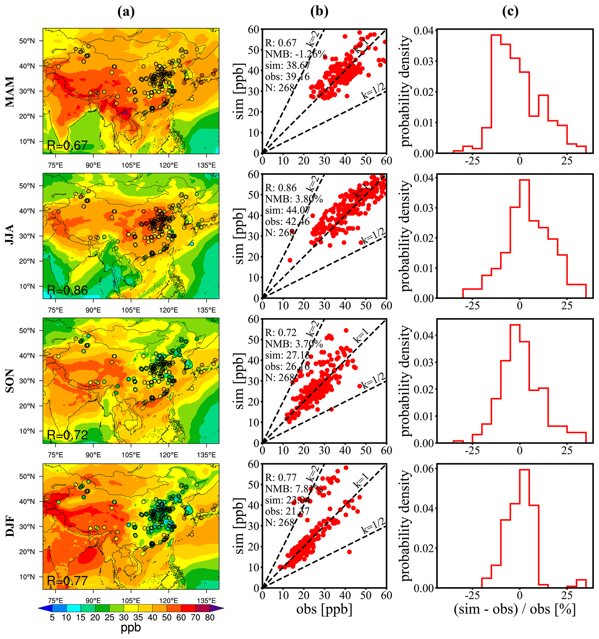
Figure 7 Comparison of surface O₃ in East Asia. (a) Spatial distribution of simulated (shaded) surface O₃ concentrations compared with observations (solid circles). (b) Scatterplots of simulated (sim) and observed (obs) seasonal mean O₃. The black dotted lines are the 2:1, 1:1, and 1:2 reference lines from left to right. (c) The probability density functions of NMB.

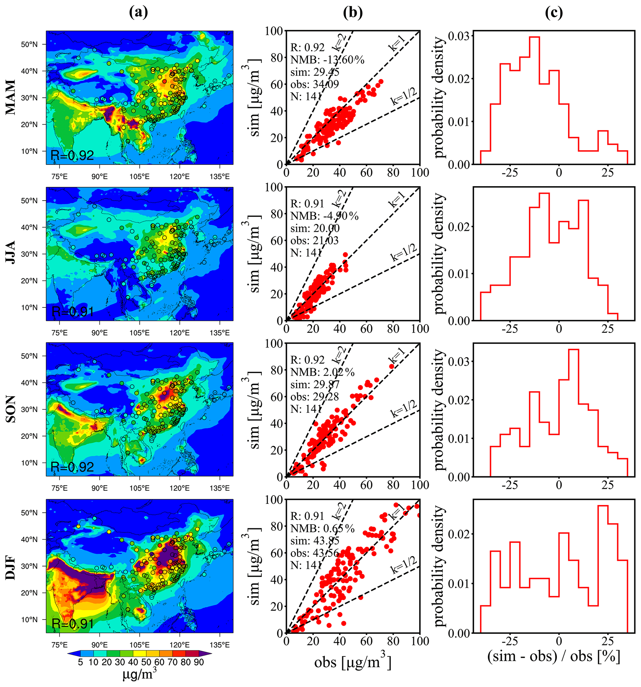
Figure 8 Comparison of surface PM_2.5 in East Asia. (a) Spatial distribution of simulated (shaded) surface PM_2.5 concentrations compared with observations (solid circles). (b) Scatterplots of simulated (sim) and observed (obs) seasonal mean PM_2.5. The black dotted lines are the 2:1, 1:1, and 1:2 reference lines from left to right. (c) The probability density functions of NMB.

Figure 8 displays that the seasonal mean simulated PM_2.5 concentration is between 20 and 43.85 µg/m³, while the observed data range from 21.03 to 43.56 µg/m³ in EA. The model shows good spatial correlations with observations and little seasonal bias, with R values ranging from 0.91–0.92 and NMB values within ±15 %. The frequent spring dust storms in northern China are an important reason for the larger PM_2.5 biases in MAM. GNAQPMS reproduces the spatial distribution of PM_2.5, including low concentrations over western China and high concentrations over eastern China, as well as 5–30 µg/m³ concentrations over the western Pacific due to sea salt. The North China Plain, central China, and the Sichuan Basin are the major hotspots, and PM_2.5 concentrations reach a maximum during DJF, with average concentrations above 90 µg/m³, which is related to stronger gradients in population density in these regions and more fossil fuel combustion for heating in DJF. Compared with that of O₃ NMBs, the probability density function (PDF) of PM_2.5 NMBs is not centralized and shows a non-normal distribution, as displayed in Fig. 8c, especially in DJF.

3.2.2 Europe

Figure 9 shows the validation of GNAQPMS simulations against EMEP observations. GNAQPMS captures the distribution of the surface layer O₃ concentration fairly well. The seasonal pattern of O₃ in Europe is characterized by higher values in MAM and lower values in SON. The high ozone area is mainly located in southern Europe (especially near Italy and Greece), and the peak ozone concentration is up to 40 ppb near the Mediterranean in JJA. The model reproduces the ground-based north–south gradient. The seasonal R values are all above 0.7 except 0.49 in MAM, and NMB values range from 4.6 % to 14.97 % with a relative overestimation during DJF in northern and western Europe. This performance is similar to MOZART (R=0.53–0.55, NMB = −19 %–6 %) and RADM2 (R=0.49–0.58, NMB $=-$33 % to −23 %) model simulations over Europe in Mar et al. (2016). The PDF in Fig. 9c shows that the NMBs in MAM and DJF are most frequently between 0 % and 10 %, and those in JJA and SON approximately obey a normal distribution.

Figure 9 Same as Fig. 7 but in Europe.

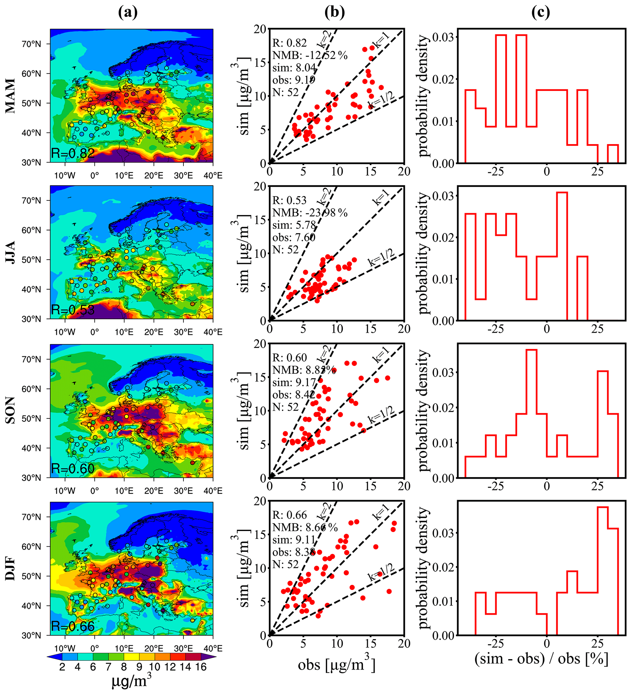
Figure 10 Same as Fig. 8 but in Europe.

The seasonal observed and simulated station PM_2.5 values are within 10 µg/m³ in Europe, as shown in Fig. 10. Mean values of PM_2.5 in Europe are fairly similar in all seasons, with a slightly lower concentration in JJA. There is no significant model bias in the seasonal mean concentrations except for a 20 % low bias in JJA. The model does not capture the observed high values in southern and central Europe during JJA. During the other three seasons, the maximum PM_2.5 in central Europe is well pronounced. The annual NMB value of −4.47 % in Table S2 at EMEP sites is less than the previously mentioned negative biases of −30.4 % in the WRF/Polyphemus model (Zhang et al., 2013) and −19.7 % in the CAMx model (Karamchandani et al., 2017).

3.2.3 North America

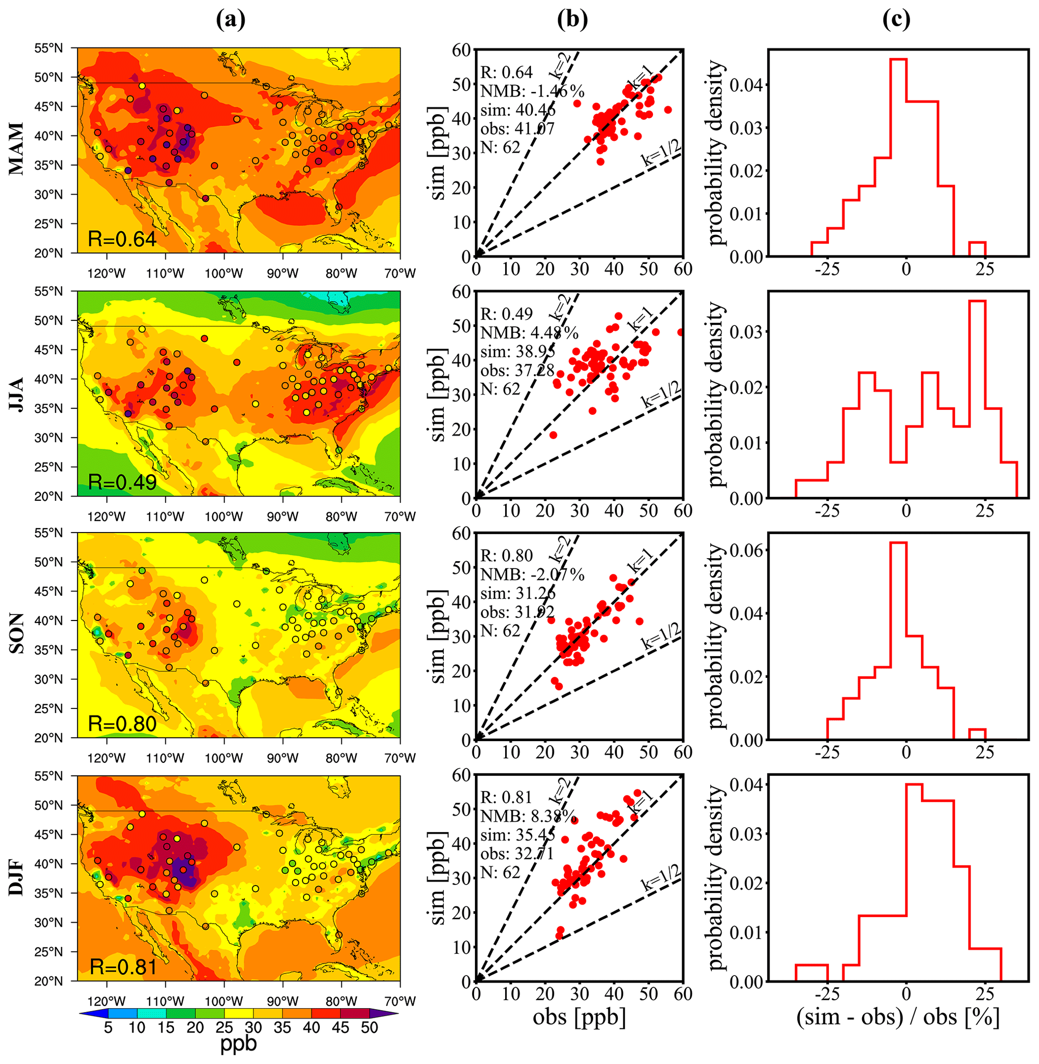
Figure 11 Same as Fig. 7 but in the United States.

Figure 11 shows the seasonal mean surface O₃ concentration in the US compared with observations from EPA network sites. The seasonal R values are between 0.49 and 0.81, with slightly poor spatial correlation in JJA, and NMB values range from −2.0 % to 8.38 %. The seasonalities of ozone in the eastern and western US are inconsistent. The model can simulate the high tail of the O₃ distribution in the western US during MAM and DJF but tends to overestimate O₃ levels by approximately 5–10 ppb in the eastern US during JJA, which also always appears in other regional or corresponding large-domain CMAQ or GEOS-Chem simulations (Hogrefe et al., 2018; Fiore et al., 2002; Guo et al., 2018). Several small-scale high-value stations in western cities, notably in California, are underestimated, which are affected by the coarser model resolution relative to finer regional resolution. In general, the simulation level in the US matches well with levels of other regional models (Hogrefe et al., 2018; Nopmongcol et al., 2017). As shown in Fig. 11c, the NMBs in MAM and SON are within ±5 % and are normally distributed.

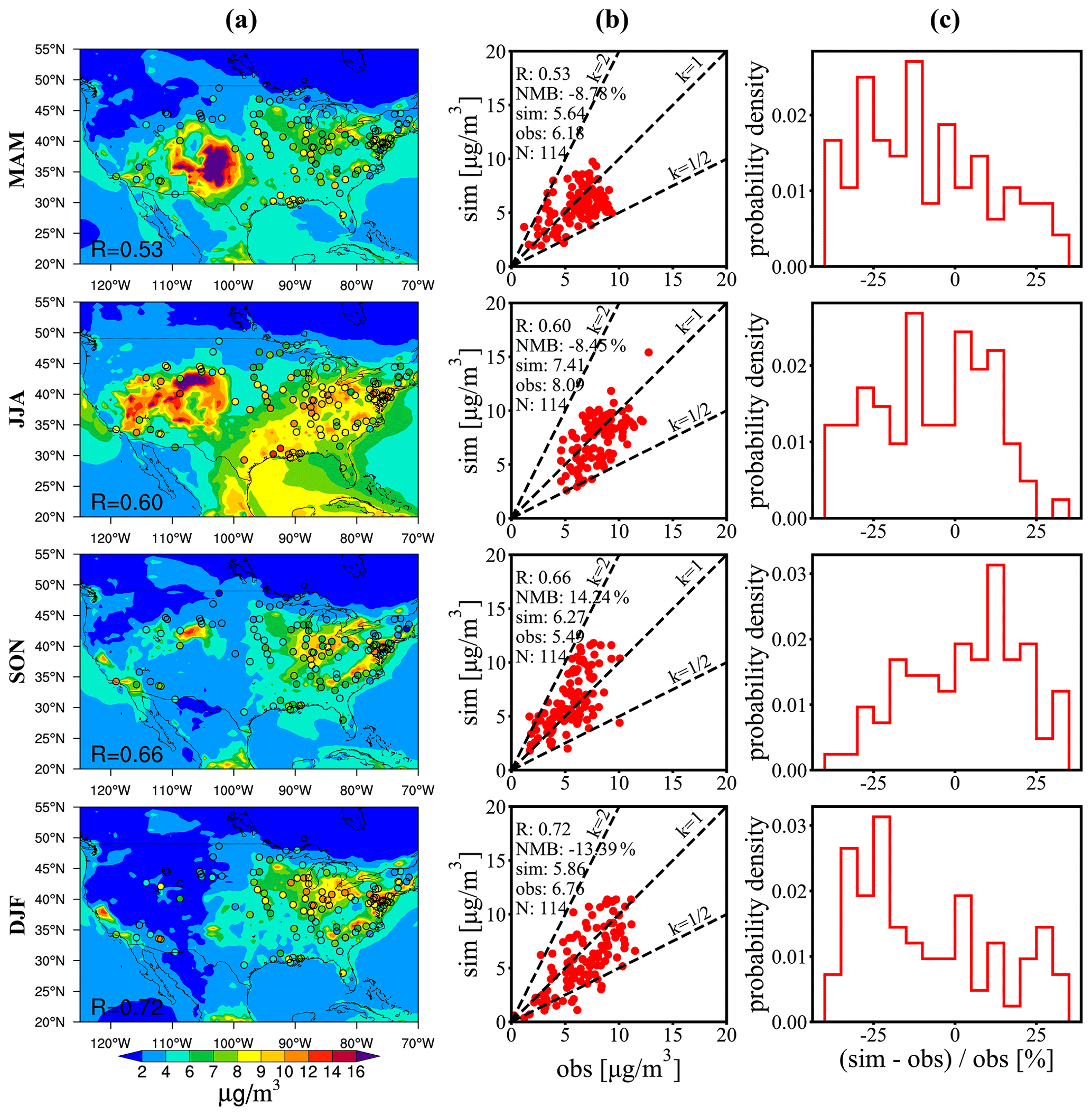
Figure 12 Same as Fig. 8 but in the United States.

As shown in Fig. 12, the seasonal mean modeled surface PM_2.5 concentrations over the US are between 5.64 and 7.41 µg/m³. Similar to Europe, the seasonal observed and simulated PM_2.5 concentrations are within 9 µg/m³, and the seasonal variation is inconspicuous. The US can be split into the western and eastern parts of the country for discussion. In the west, the hotspot is located in the central region and peaks during MAM. In the east, the larger high-value zones reach a maximum during JJA. Except for SON, there is a slight tendency to underestimate the concentration. This performance over the US is similar to the GEOS-Chem results in Kim et al. (2015).

4 Results of S-R relationships

4.1 S-R relationships in the surface layer

We have evaluated annual and seasonal model performance thoroughly. This laid a good foundation for the S-R relationship analysis that follows. The contributions of different source regions are calculated and discussed in this section.

4.1.1 Surface PM_2.5 source–receptor relationships

PM_2.5 has anthropogenic and natural emission sources. All of sand dust and sea salt are considered to be from natural emissions. Figure 13 shows the annual and seasonal estimates of the contributions to surface PM_2.5 (in percent) from source regions to receptor regions on a global scale. The transport distance of surface PM_2.5 is limited. Local and natural sources play major roles, with contributions of nearly more than 90 %, while the contribution of external sources is small (Fig. 13e). The yearly contribution from EA to itself is 77.4 %, and the contributions from natural emissions, SAS, and SEA to EA are 18.2 %, 2.0 %, and 1.0 %, respectively. Sources in the EA explain approximately 3.6 % of the PM_2.5 concentration in RBU and 2.5 % in SEA. The PM_2.5 in EUR is generally more sensitive to local emissions (68.2 %) than to natural emissions (27.3 %). OCN and RBU also contribute 2.4 % and 1.1 % to EUR, respectively. These contributions show seasonal variations. As shown in Fig. 13a–d, local emissions from EA contribute approximately 59.9 %–93.9 % of the surface PM_2.5 concentration over EA in all seasons, and local emissions from SAS contribute approximately 33.8 %–95.4 % over SAS, which peaks in DJF due to greatly increased biomass and fossil fuel burning for heating. The export of PM_2.5 from EA contributes approximately 0.9 %–11.6 % over RBU and CAS, and these contributions are high in DJF, mainly due to the large emissions and concentrations of PM_2.5. Similarly, exports from SAS contribute 0.1 %–9.0 % over EA and SEA in the four seasons due to westerly winds. Desert dust of MDE, NAF, and CAS (Mongolia is included in CAS) plays an important role in MAM and JJA, which is caused by their desert terrain, more dust storm activity, and higher PM_2.5 surface concentration. Because marine emissions can also make a considerable contribution to air pollution, local sea salt emissions cause natural emissions to make more than 90 % and 75 % contributions to NPO and OCN, respectively. Antarctica (SPO) has a low population, and transportation sources are also small, so the contribution of natural sources is larger than that in other regions. Local anthropogenic sources contribute more than 50 % to the PM_2.5 concentrations in EA, RBU, SEA, SAS, EUR, NAM, and SAM and even exceed natural emissions. SAS contributes 2 % to the EA surface PM_2.5 contribution annually, while EA contributes 0.2 % to SAS. Although SAS is controlled by the South Asian winter monsoon in DJF, the northeast wind in DJF is weaker than the southwest wind in JJA. In addition, the PM_2.5 concentration of SAS in DJF is higher than that in JJA, so the contribution to EA from SAS is largest in DJF among the four seasons. These midlatitude regions are dominated by westerly winds and therefore can make a greater contribution to the downwind receptor region. PM_2.5 can also transport across regions between high latitudes and low latitudes, such as PM_2.5 from EUR traveling south to NAF, especially in JJA. Because of the deposition, PM_2.5 mainly contributes to its surrounding receptor regions and cannot be transported over long distances in the surface layer. The near-surface downwind transport is not easy to cross the Pacific and the Atlantic. For example, only 0.1 % of PM_2.5 in NAM is from EA and 0.2 % of PM_2.5 in EUR is from NAM annually.

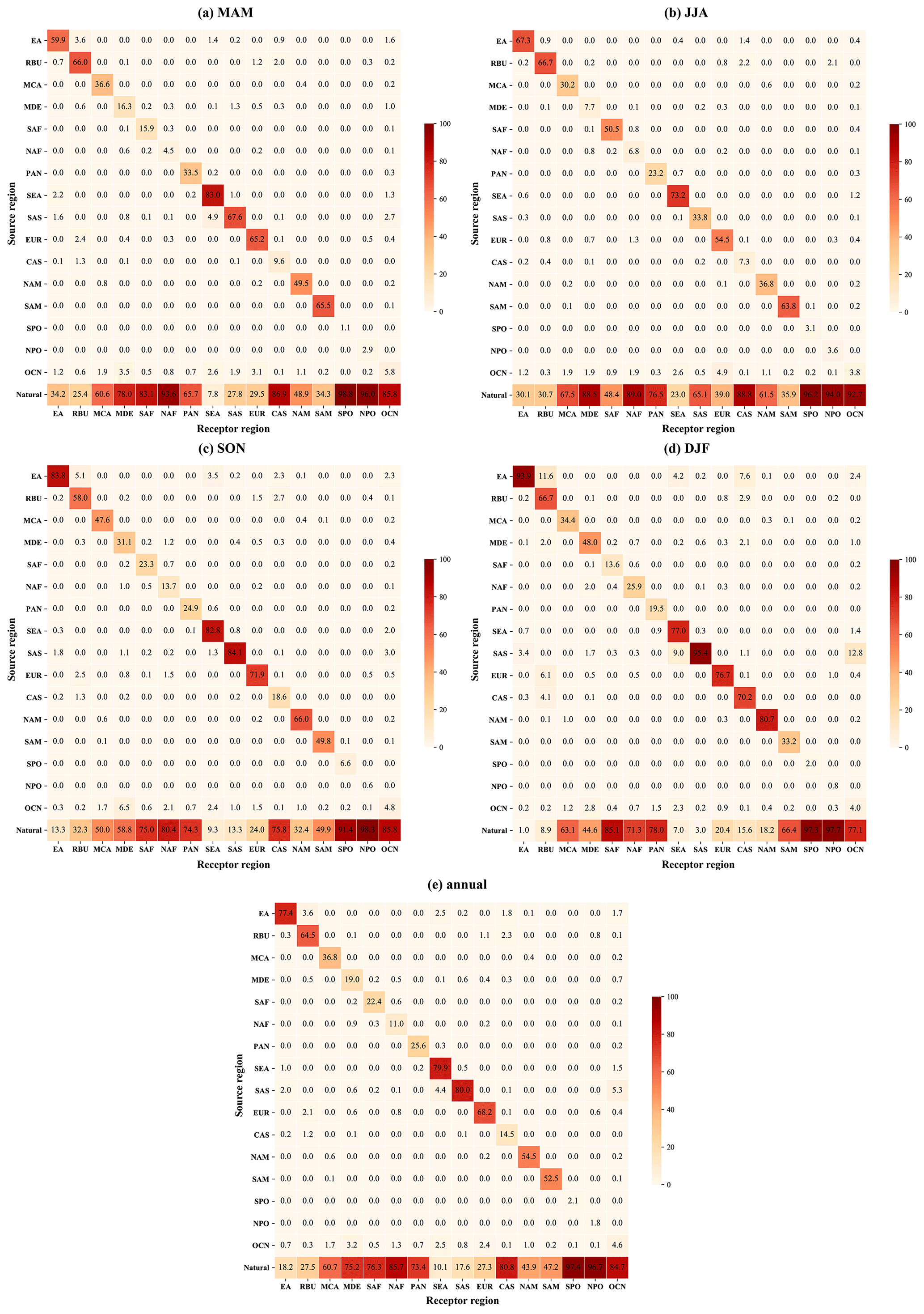
Figure 13 Annual and seasonal estimates of the contributions to surface PM_2.5 (%) from source regions to receptor regions.

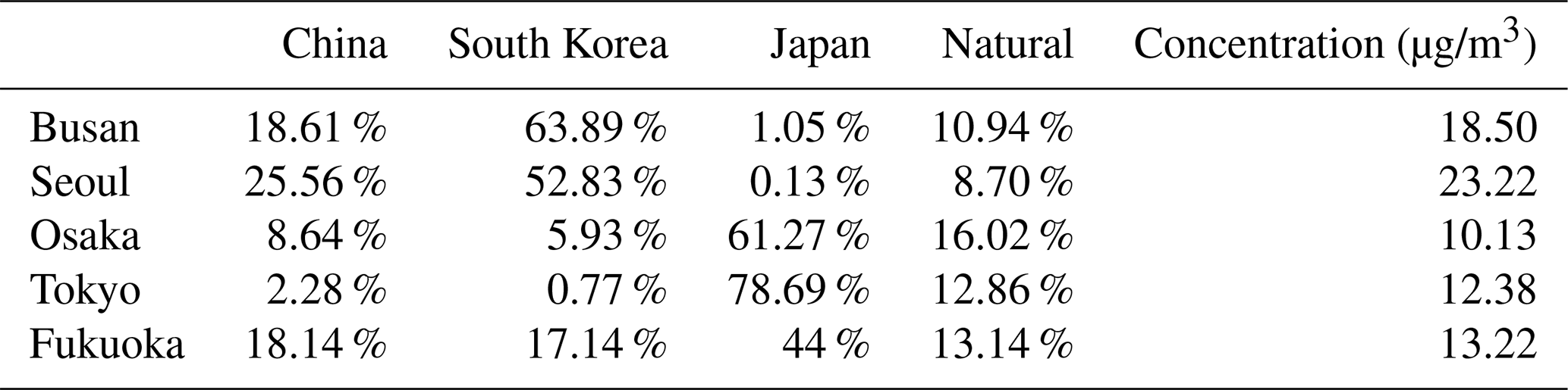
To better quantify the S-R relationships for PM_2.5 in EA, we split EA into China, Japan, South Korea, and North Korea. We select five cities: Busan (35.09^∘ N, 128.58^∘ E), Seoul (37.55^∘ N, 126.97^∘ E), Osaka (34.07^∘ N, 135.05^∘ E), Tokyo (35.7^∘ N, 139.77^∘ E), and Fukuoka (33.6^∘ N, 130.58^∘ E) to compute the yearly contributions of China, South Korea, Japan, and local anthropogenic emissions. As shown in Table 2, local anthropogenic emissions are the most prominent source of surface PM_2.5 in Busan, Seoul, Osaka, Tokyo, and Fukuoka, which contribute 63.89 %, 52.83 %, 61.27 %, 78.69 %, and 44 %, respectively. Long-term studies that analyzed long-range transport of PM_2.5 seasonally or annually in South Korea and Japan reported that local contributions ranged from 30 % to 60 %, depending on the season, and local contribution was higher in the metropolises of Japan and South Korea (Kim et al., 2017; Yim et al., 2019; Lee et al., 2017). There is no significant difference between their studies and our results. Natural emissions explain ∼ 10 % of PM_2.5 concentrations in the five cities. China makes a greater contribution to Busan and Seoul (18.61 % and 25.56 %, respectively) in closer South Korea than to Osaka and Tokyo (8.64 % and 2.28 %, respectively) in farther Japan. Compared with the other two cities in Japan, Fukuoka is located in southwestern Japan and is closer to China and South Korea; thus, the contributions from China and South Korea reach 18.14 % and 17.14 %, respectively. This is also related with meteorological conditions controlled by westerly winds, as mentioned above. China's contribution to South Korea, which is closer to China, is generally greater than that to Japan. Japan is located in the downwind area of South Korea, so Japan's contribution to Busan and Seoul (1.05 % and 0.13 %, respectively) is less than that of Korea to Osaka, Tokyo, and Fukuoka (5.93 %, 0.77 %, and 17.14 %, respectively).

Table 2 Contributions from China, South Korea, and Japan to surface PM_2.5 (in percent) in five cities.

4.1.2 Surface O₃ source–receptor relationships

Different from PM_2.5, O₃ S-R relationships are affected by many precursors that are emitted, reacted, and then generated, which are also attributed to the influence of photochemical reactions, and show a stronger nonlinearity. In our S-R module, primary pollutants and secondary aerosols are tagged by their or their precursor emitting locations, and other secondary species like O₃ are tagged by the produced locations. Therefore, we calculate the O₃ contribution of a source region that was chemically produced inside this source region and then transported to another receptor region, inevitably including amounts of O₃ produced inside this source region from precursors emitted in neighboring source regions and transported to this source region. As shown in Fig. 14, sources from EA, MCA, MDE, SAF, SEA, SAS, NAM, and SAM have contributed more than 50 % to themselves in the surface layer. Similar to PM_2.5, the transport of O₃ in the midlatitude regions of the Northern Hemisphere is also controlled by the prevailing westerly wind. The contribution of RBU surface O₃ from the EUR source region averages 8.3 % over the year, while the contribution of EUR surface O₃ from the RBU source region averages 6.5 %. Compared with PM_2.5, O₃ has a longer surface transport distance and greater contribution of transboundary transport, which is above 30 % and generally approximately 50 %. Nearly 25 % of global anthropogenic NO_x emissions originated from shipping, plus the NO_x transported to OCN, and the influence of local photochemical reactions on O₃ is significant in OCN (38.7 %). O₃ can be transported across the ocean through the surface layer. The export of O₃ from NAM contributes 9.2 % of surface O₃ concentrations in EUR under the control of the westerly jet crossing the North Atlantic and contributes approximately 6 % in MCA due to northerly winds. NAM also contributes significantly (10.2 %) to NPO O₃. Affected by the South Asian monsoon, O₃ originating from SAS can be transported to EA (8.9 %) and across the Bay of Bengal to SEA (2.9 %). Sources in EA explain approximately 3.6 % of O₃ effectively crossing the North Pacific to NAM. The exported surface O₃ from RBU can travel to EUR, with a relative contribution (6.5 %) exceeding that to NAM (5.4 %) and EA (2.8 %). Surface concentrations over NPO have a close association with emissions from source regions. The largest contribution in NPO is from RBU, and the contributions from EUR and NAM are similar in magnitude. Basically, O₃ is transported to NPO from every source region, even from PAN in the Southern Hemisphere. The contribution of the top boundary is large in SPO due to the low tropopause of SPO and the simplified treatment of the stratosphere, while the contribution of the top boundary is smaller in Northern Hemisphere receptor regions compared with the contribution of photochemical reactions.

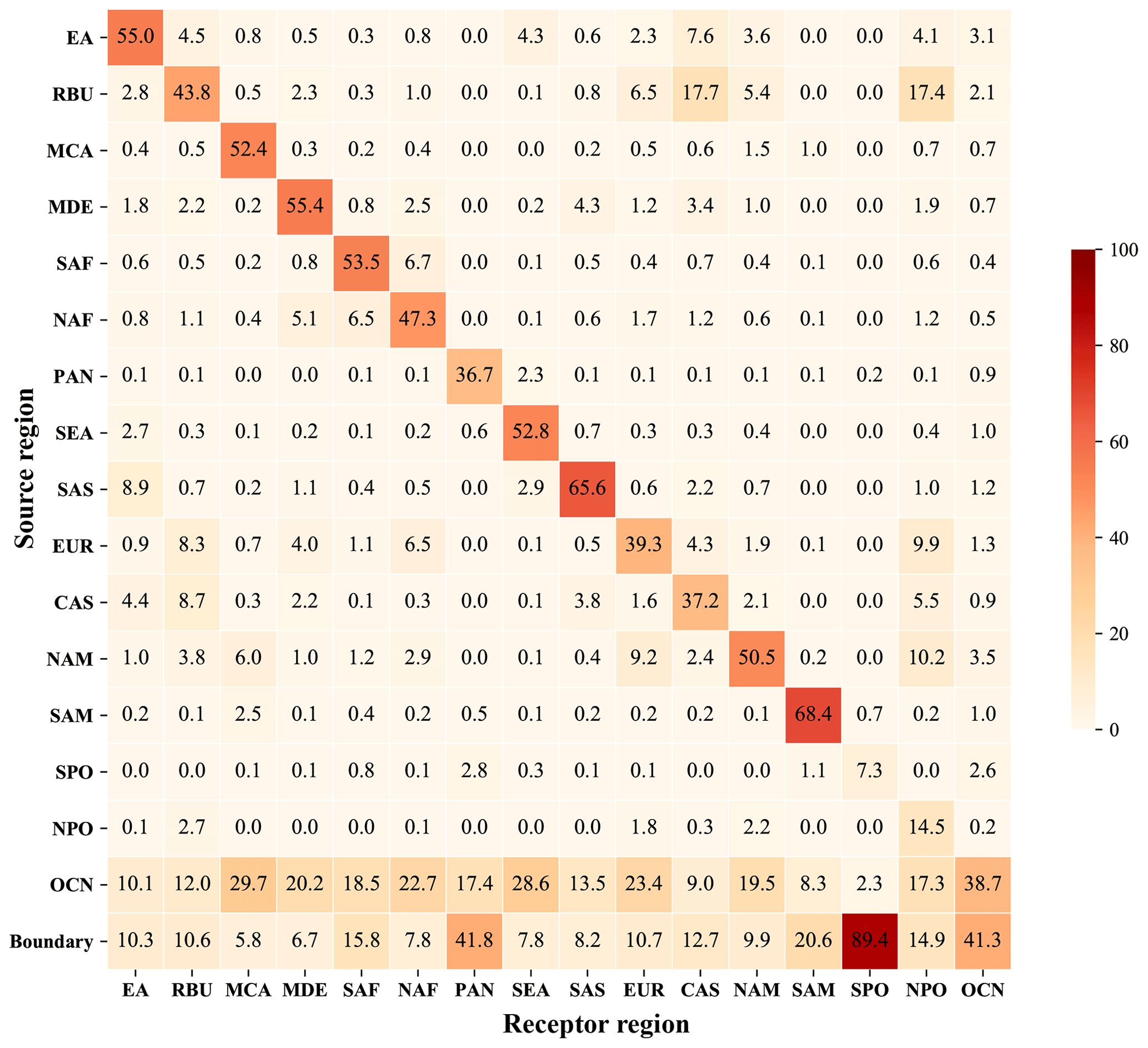
Figure 14 Annual estimates of the contributions to surface O₃ (%) from source regions to receptor regions.

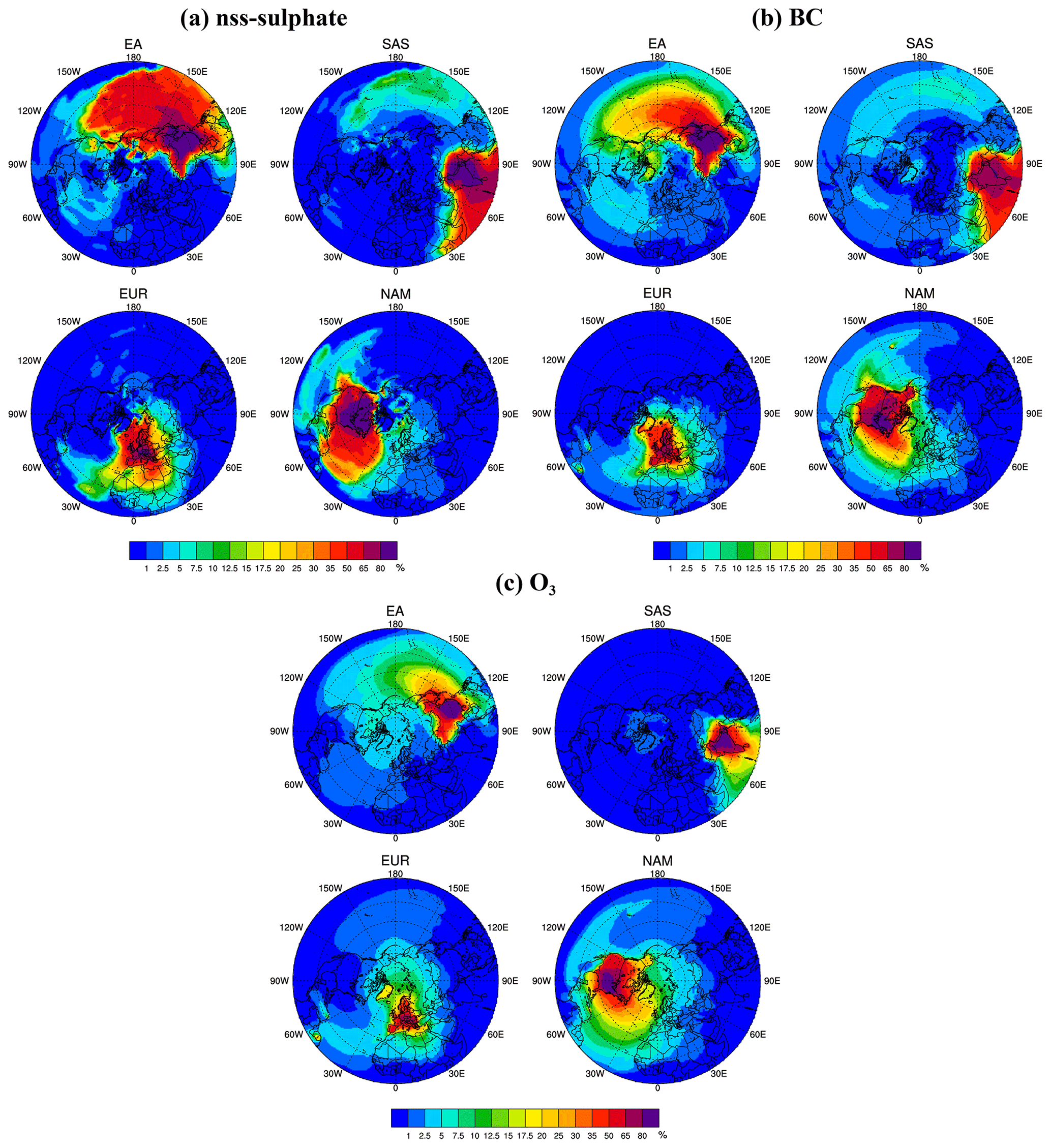
Figure 15 Spatial distribution of source region contributions to (a) nss-sulfate; (b) BC concentration within the PBL and (c) O₃ (%) in the surface layer.

Then, we choose 4 source regions to focus on: EA, SAS, EUR, and NAM. Figure 15c presents the spatial distribution of the relative contribution to surface O₃ from these regions. Due to westerly winds in the middle latitudes, non-local source transport accounts for less than 20 % in the eastern part of EA and NAM but contributes approximately 30 % in the western part of NAM and more than 50 % in western EA, considering the lifetime of O₃ and meteorology, where surface O₃ is vulnerable to the influence of external sources. As shown in Fig. 15c, surface O₃ can be transported on a hemispheric scale. Exports from EUR can explain approximately 5 %–10 % over North Asia and the northeast Atlantic, and approximately 5 %–15 % over NPO. Surface O₃ can even be transported across NPO to the North Pacific, making a nearly 5 %–7.5 % contribution. Similarly, O₃ from EA can be transported south to SEA, west to the North Pacific, north to RBU, and across NPO to the North Atlantic.

4.2 Nss-sulfate and BC source–receptor relationships within the PBL

Figure 16 displays the yearly relative contributions to nss-sulfate and BC within the PBL. The transport characteristics of nss-sulfate and BC are similar to those of PM_2.5, exhibiting a dominant traveling from west to east. However, the relative contribution from source regions varies by pollutants, regions, and heights. The contributions of long-range transport explain approximately 15 %–30 % of nss-sulfate and 20 %–35 % of BC in EA, SAS, EUR, and NAM. Nss-sulfate is one of the secondary aerosols that is mainly formed by SO₂ oxidation; hence, the concentration of nss-sulfate is mostly affected by source regions with high anthropogenic SO₂ emissions, such as EA, SAS, EUR, and NAM. The exports from EA and EUR are responsible for approximately 20 % of nss-sulfate within the PBL over RBU, the sum of which is comparable to the contribution from RBU local sources (40.9 %). The non-local source contribution is similar to the results in Yang et al. (2017a) based on CESM for 2010–2014, where the contributions of EA and EUR to RBU are 15 % and 12.5 %, respectively. EA and SAS each account for more than 20 % of nss-sulfate over SEA, and their sum is larger than the local contribution from SEA (37.2 %). Nss-sulfate from EA can be effectively transported to the surrounding regions with considerable contributions to RBU (17.4 %), SEA (22.2 %), CAS (18.3 %), and OCN (21.4 %). The NPO nss-sulfate is more sensitive to emissions from EUR (45.2 %), RBU (14.4 %), and NAM (8.5 %) than local emissions (7.1 %). Distinct from nss-sulfate, BC is the primary aerosol, and its concentration is directly related to BC source emissions, such as biomass burning and gas flaring. Therefore, the contribution of “other”, which considers natural emissions in RBU, SAF, PAN, SEA, and SPO, to BC is relatively large. RBU, EUR, and NAM have a relative contribution of nearly 40 % to NPO BC within the PBL. The contribution of NAM nss-sulfate and BC concentration within the PBL from the EA source region is 1.6 % and 5.7 %, respectively. The contribution of EUR nss-sulfate and BC concentration within the PBL from the NAM source region is 3.6 % and 6.7 %, respectively. The transport distances of nss-sulfate and BC in the PBL are still limited, and they need to be uplifted into the upper free troposphere for longer-distance transport.

Figure 16 Annual estimates of the contributions to (a) nss-sulfate and (b) BC (%) within the PBL from source regions to receptor regions. “Other” refers to the effects of natural emissions and the boundary layer.

Figure 15a–b display the spatial plots of yearly relative contributions to nss-sulfate and BC concentration within the PBL for the EA, SAS, EUR, and NAM receptor regions. Relatively speaking, BC is transported longer distances than nss-sulfate, which can also be found in Fig. 16. Note that the relative contribution in Fig. 16 is the annual mean contribution of the entire region. The influences of both BC and nss-sulfate extend throughout more than half of the Northern Hemisphere, as shown in Fig. 15. BC in the Arctic has always been a concern, and it is clear that the largest contributions over NPO within the PBL are from EUR, which is similar to previous studies (Sobhani et al., 2018). The concentrations of BC are dominated by local sources in eastern China, while more than 50 % of the BC concentration within the PBL in western China is from emissions outside China. EA emissions have up to 7.5 %–12.5 % and 7.5 %–17.5 % contributions to the western US and western Canada BC concentrations, respectively. The yearly contribution to the western US is comparable to the average contribution of 8 % over the western US based on the CESM model in Yang et al. (2017b). Among regions outside EA, EA makes a very large contribution to the Northwest Pacific, with relative values between 35 % and 50 %. Due to the influence of the southwest monsoon in summer and northeast monsoon in winter, the BC from SAS can be transported southward and westward, with a wide range of transport. Because EUR is close to NPO, the contribution to some parts of NPO could reach up to 35 %. In addition to being transported to EUR, BC from NAM can also travel westward, affecting the northeast Pacific. Although nss-sulfate travels shorter distances than BC, its relative contribution to the receptor regions is greater. Nss-sulfate from the EA source region contributes almost 50 % to the North Pacific, and nss-sulfate from SAS could also make an approximately 7.5 % contribution to the North Pacific. There is significant southward sulfate transport to NAF from EUR. Moreover, the influence of nss-sulfate from NAM extends to the northwest Pacific, ranging from 35 %–50 %. Due to the elevated topography of southwest China, both BC and nss-sulfate from SAS cannot reach eastern China within the PBL.

4.3 Comparison with HTAP results

Despite wide variations in nss-sulfate and BC surface concentrations among the different models, S-R relationships have some similar characteristics. We compare the S-R relationships of surface nss-sulfate and BC in our study with annual averages in 2001 from six models from part A of the HTAP report (Dentener et al., 2010), as illustrated in Fig. 17. More detailed comparisons are listed in Table 3. Because the height of the surface layer in the models in the HTAP report is not given, we also evaluated the contributions within the PBL. Although the surface contributions from local regions in our study are higher than the HTAP results, they are of the same magnitude. Compared with that of nss-sulfate, the contribution of BC in the surface layer or in the PBL in our study is closer to that in HTAP, which may be related to the inactive chemical properties of BC. Nss-sulfate, as a secondary pollutant, its S-R relationships in the surface layer are affected by precursors, photochemical processes, physical loss processes, and mixing during transport. Therefore, there are some disagreements on surface nss-sulfate contributions. However, the results of nss-sulfate within the PBL are more consistent with the results in the HTAP report. For the transport within the PBL, the contribution from local sources is smaller than that for surface transport due to the inseparable transport height and distance.

Figure 17 Contributions of (a) nss-sulfate and (b) BC in the surface layer and within the PBL from the HTAP report and GNAQPMS-SM. HTAP results with red error bars are based on the annual averages in 2001 from six global models. GNAQPMS-SM results in the surface layer are shown as black dots, and those within the PBL are shown as blue dots. (The region shown in the x axis of the horizontal coordinate is the result of HTAP division, which is slightly different from the region defined in this paper.)

Table 3 Relative contributions (%) compared with those in the HTAP report (Dentener et al., 2010). The median and range of the annual averages of the six models are given below.

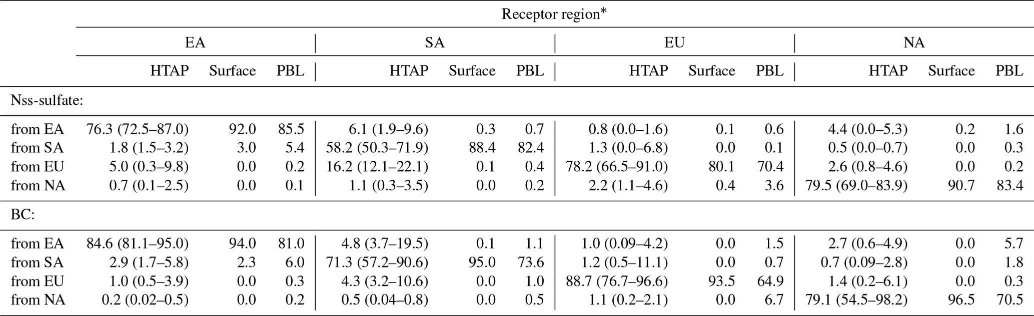
^* Note that there are some different definitions between the regions used in the table heading and in our study. The definitions of the regions in the table are stipulated by HTAP. Approximately, EA in HTAP is equal to EA in this paper, SA to SAS, EU to EUR, and NA to NAM.

We also compare the contributions to receptor region NAM and EA surface O₃ with the Fiore et al. (2009) study which is related to HTAP report studies as shown in Fig. S3. When extrapolated to a 100 % source contribution, the Fiore et al. (2009) results suggest that EUR and EA contribute from 0.3–2.1 and 0.3–2.0 ppb to surface O₃ in NAM and EUR and NAM contribute from 0.4–2.9 and 0.3–2.0 ppb to surface O₃ in EA, respectively. Although most of our results are within the range, NAM's contributions to EA in our results are consistently lower, and the contributions from EUR and EA to NAM are lower in JJA.

In addition to the uncertainties caused by different processes represented in models, different simulation years, and S-R calculation methods, emission inventories could also affect the S-R relationship. With the rapid development of the economy in the past 20 years, the emissions in many source regions have changed significantly, which has influenced the spatial distribution of pollutants and the S-R relationship. The uncertainties of pollutants between emission inventories are large and can affect our comparison of S-R relationships. The inadequate vertical grid resolution cannot properly resolve plume gradients which could also introduce uncertainties (Eastham and Jacob, 2017). Furthermore, when the horizontal resolution is coarser, it may be responsible for the lower contribution from source regions to themselves because of the absence of some local point sources. Additionally, due to the average effect caused by the coarser grid cell, the transport distance of pollutants could be overestimated, and the non-local source contribution could also be overpredicted. Finally, the different definitions of source region between this study and HTAP can also influence the results. Because cleaner Greenland is included in EUR and cleaner Canada is included in NAM in this study compared with EU and NA in HTAP, the regional and annual average surface concentrations in Europe and North America are lower in our simulation.

4.4 Comparison with emission sensitivity simulation results

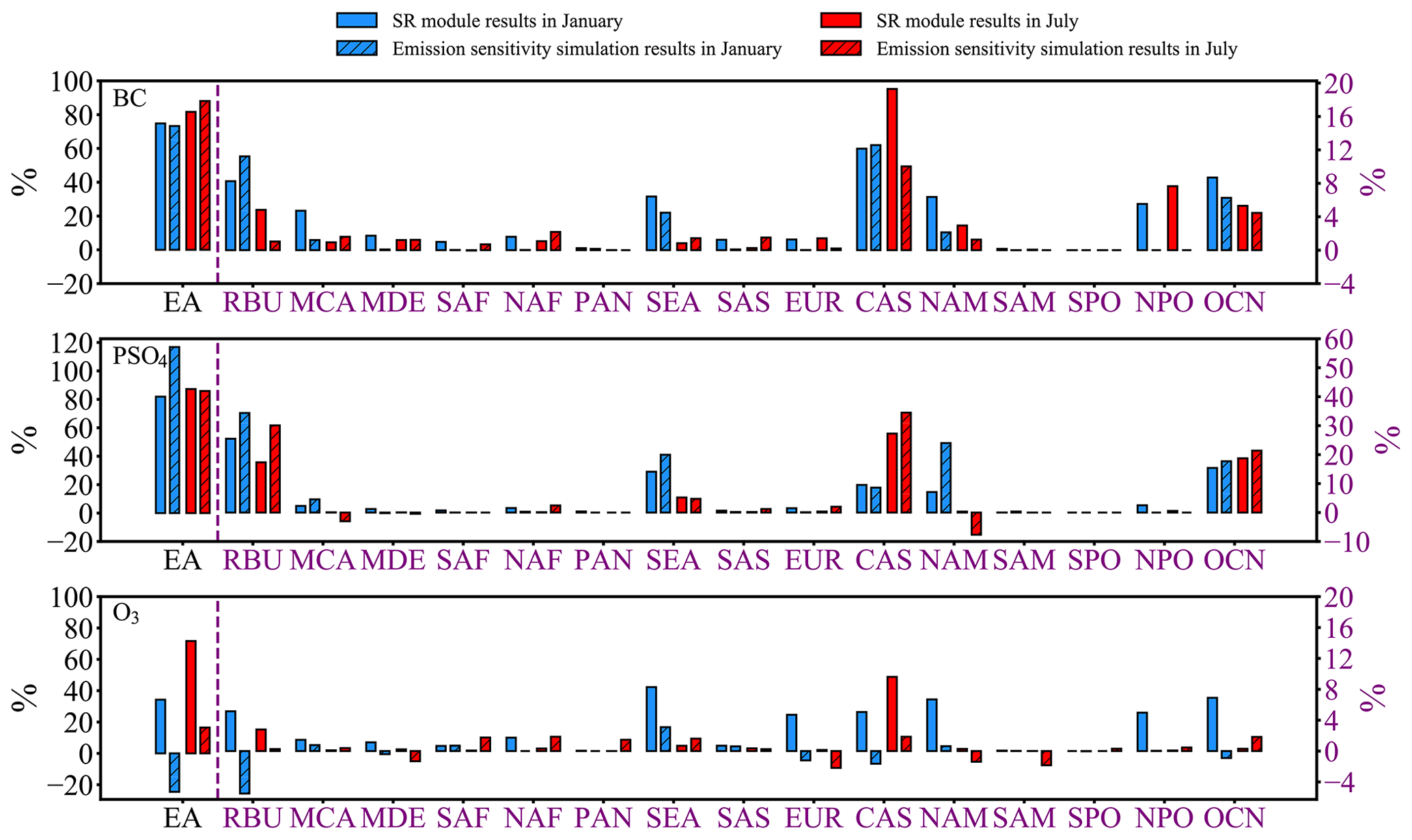
Figure 18 BC, nss-sulfate within the PBL and surface O₃ contribution from S-R module results and full response from emission sensitivity simulation results from EA source region in January and July. The y axis of receptor region EA is the coordinate axis on the left shown in black, and the y axis of other receptor regions is the coordinate axis on the right shown in purple.

EA is an emission hotspot in the world. To better isolate the S-R calculation methods' effects of other possible reasons, e.g., horizontal and vertical resolution, emission inventories, and models, we have carried out an additional emission sensitivity simulation with 20 % reduction of anthropogenic emissions in EA in January and July of 2018. Pollutant response is defined as the ratio between the concentration difference between the baseline scenario and the perturbation scenarios and the concentration of the baseline scenario, based on the average of all grid cells in the receptor region. We make the hypothesis that −20 % perturbation responses can be extrapolated towards −100 % perturbation range, as an approximation of full response from the source region EA and compare with our S-R module results as shown in Fig. 18. The S-R module results are consistently higher than the emission sensitivity simulation results, except in few regions, partly reflecting the S-R module method pays attention to all global sources instead of anthropogenic component from regions we focus on, the conclusion of which is consistent with HTAP report (Dentener et al., 2010). There is no significant difference for BC, suggesting that BC levels are largely driven by local emissions and long-range transport. Nss-sulfate and O₃ responses exist negative values, suggesting that regional nss-sulfate and O₃ levels are also driven by precursor emissions besides local emissions and long-range transport. Compared with O₃, the difference between two methods on nss-sulfate is smaller. O₃ shows more negative response and larger difference. Especially in receptor region EA in January, the O₃ responses are negative due to the strong nonlinearity in O₃ chemistry. In our S-R module method, all contributions are strictly positive. However, in emission sensitivity method, the impacts are computed and may appear negative values, particularly in higher emission regions in DJF, which is also reported in Li et al. (2008) and Grewe (2004). The differences between two S-R revealing methods in estimated S-R relationships of secondary aerosols and O₃ are mainly due to the ignorance of the nonlinearity of pollutants during chemical processes.

5 Summary and future plans

In this study, an online S-R relationship module based on a tagged tracer approach was coupled into the global tropospheric model GNAQPMS. The developed model can help us better quantify the contributions of multiple air pollutants from various source regions at the same time without introducing the nonlinear error of atmospheric chemistry. A global high-resolution (0.5^∘ × 0.5^∘) simulation of air pollutants in 2018 was conducted with EDGAR v5.0 and other emission inventories. The global tropospheric atmospheric chemistry source–receptor model will be useful to clarify the S-R relationships of various pollutants from a global perspective and help create a link between the scientific community and policymakers.

GNAQPMS generally captures the distribution and seasonality of air pollutants at global and regional scales (EA, EUR, and NAM). The model reproduces the seasonal distribution of surface O₃ at background stations from WDCGG and vertical variation of ozonesonde observed O₃ in the middle–lower troposphere from WOUDC. The overestimation of O₃ mixing ratios in the upper troposphere and stratosphere in the tropics, midlatitude, and polar region of the Southern Hemisphere could be attributed to the lack of explicit simulation of stratosphere chemistry and the simplified treatment of the exchange of stratosphere with troposphere in GNAQPMS. The mean concentration of tropospheric OH is 11.9×10⁵ molecules/cm³, which is similar to previous studies. The seasonalities of NO₂ columns and AOD are well captured. The concentration of surface O₃ is in good agreement with observations from global background and urban–rural sites, with spatial correlations ranging from 0.49 to 0.87 and NMB values ranging from −2.07 % to 14.97 %. Although the model tends to underestimate the surface concentrations of NO₂, BC, OC, and sulfate, simulated PM_2.5 and SNA show strong correlations and no significant biases with observations over EA, EUR, and NAM. In general, the performance of the high-resolution global model and that of the regional model is well matched.

The relative contributions of 19 source regions to pollutants show some similarities and vary with species, regions and heights. Transport in the midlatitudes is dominated in the west–east direction under the control of westerly winds. Only a small minority of PM_2.5 can be transported across the Pacific and Atlantic through the surface layer. The PM_2.5 generated or emitted in the source region mainly contributes to itself and its surrounding regions. For the S-R relationships inside EA, local anthropogenic emissions from Busan, Seoul, Osaka, Tokyo, and Fukuoka are the major contributors to their own surface PM_2.5. Contributions from non-local sources account for approximately 20 %–55 % of surface PM_2.5. South Korea is closer to downwind of China; thus, China's contribution to South Korea is greater than that to Japan. Compared with surface PM_2.5, surface O₃ can be transported on a hemispheric scale (e.g., from PAN in the Southern Hemisphere to NPO). Non-local source transport explains approximately 35 %–60 % of surface O₃ in EA, SAS, EUR, and NAM. O₃ from EUR can be transported across NPO to the North Pacific and contributes nearly 5 %–7.5 % to the North Pacific. BC, as a primary aerosol, is directly linked to emissions. As a result, in the RBU, SAF, PAN, and SEA regions, where biomass burning emissions are large, natural emissions make a significant contribution to BC within the PBL. In contrast to BC, nss-sulfate is mainly generated by the oxidation of SO₂, the S-R relationship of which is mainly influenced by source regions with high local emissions. The contributions of long-range transport account for 15 %–30 % within the PBL in EA, SAS, EUR, and NAM. The transport distance of nss-sulfate and BC is limited in the PBL and they need to be lifted above the PBL for longer-distance transport. The contributions of long-range transport can explain less than approximately 20 % of pollutant concentrations over the midlatitude continental regions of the eastern part of EA and NAM due to the control of westerly winds, while they can explain approximately 30 % over the western part of NAM and more than 50 % over western EA.

In comparison with HTAP report results, local contributions from source regions to surface nss-sulfate and BC in GNAQPMS-SM exceed the range given in the HTAP report. When considering the relative contributions within the PBL, the local contributions decrease and are basically within the range. Compared with Fiore's results, most of our results are within the range, except that NAM's contribution to EA surface O₃ in our results are consistently lower, and the contributions from EUR and EA to NAM surface O₃ are lower in JJA. These differences may be related to different simulation years, S-R revealing methods, and emission inventories. Different regional definitions and model vertical and horizontal resolutions may also be responsible, among which the non-local source contribution could be overestimated and the local source contribution could be underestimated when the horizontal resolution is coarser. The reasons should be discussed in detail in future work. We plan to conduct a coarser horizontal resolution simulation in GNAQPMS-SM to clarify the sensitivity of S-R relationships to different resolutions. The impact of uncertainties from emissions and meteorological fields (wind field and precipitation field) on S-R relationships could also be quantified in the next step. We also plan to carry out global simulations of future and historical periods to explore the changes in S-R relationships and uncertainties, focusing on S-R relationships.

Additional emission sensitivity simulation shows a negative O₃ response in receptor region EA in January from EA. The difference between two S-R revealing methods in estimated S-R relationships of secondary aerosols and O₃ are mainly due to ignoring the nonlinearity of pollutants during chemical processes. The S-R module results are consistently higher than the emission sensitivity simulation results, except in few regions, partly reflecting the S-R module method pays attention to all global sources instead of anthropogenic component from regions we focus on.

The development of an online S-R module embedded in GNAQPMS and the analysis of global S-R relationships represent an important step for China. The S-R relationships of both primary and secondary pollutants can be calculated in one simulation. We give our opinions on the controversial topic of the intercontinental transport of pollutants. The model that we developed creates a link between the scientific community and policymakers.