the Creative Commons Attribution 4.0 License.
the Creative Commons Attribution 4.0 License.
 | 30 Nov 2021
Assessment of the ParFlow–CLM CONUS 1.0 integrated hydrologic model: evaluation of hyper-resolution water balance components across the contiguous United States
Mary M. F. O'Neill
Danielle T. Tijerina
Laura E. Condon
Reed M. Maxwell
Recent advancements in computational efficiency and Earth system modeling have awarded hydrologists with increasingly high-resolution models of terrestrial hydrology, which are paramount to understanding and predicting complex fluxes of moisture and energy. Continental-scale hydrologic simulations are, in particular, of interest to the hydrologic community for numerous societal, scientific, and operational benefits. The coupled hydrology–land surface model ParFlow–CLM configured over the continental United States (PFCONUS) has been employed in previous literature to study scale-dependent connections between water table depth, topography, recharge, and evapotranspiration, as well as to explore impacts of anthropogenic aquifer depletion to the water and energy balance. These studies have allowed for an unprecedented process-based understanding of the continental water cycle at high resolution. Here, we provide the most comprehensive evaluation of PFCONUS version 1.0 (PFCONUSv1) performance to date by comparing numerous modeled water balance components with thousands of in situ observations and several remote sensing products and using a range of statistical performance metrics for evaluation. PFCONUSv1 comparisons with these datasets are a promising indicator of model fidelity and ability to reproduce the continental-scale water balance at high resolution. Areas for improvement are identified, such as a positive streamflow bias at gauges in the eastern Great Plains, a shallow water table bias over many areas of the model domain, and low bias in seasonal total water storage amplitude, especially for the Ohio, Missouri, and Arkansas River basins. We discuss several potential sources for model bias and suggest that minimizing error in topographic processing and meteorological forcing would considerably improve model performance. Results here provide a benchmark and guidance for further PFCONUS model development, and they highlight the importance of concurrently evaluating all hydrologic components and fluxes to provide a multivariate, holistic validation of the complete modeled water balance.
- Article
(29399 KB) - Full-text XML
-
Supplement
(3857 KB) - BibTeX
- EndNote


Explicitly modeling the terrestrial water cycle at the global scale and at high resolution has recently been referred to as a “grand challenge in hydrology” (Bierkens et al., 2015; Wood et al., 2011), an undertaking that has excited the hydrologic community and encouraged the development of large-scale modeling efforts, workshops, and working groups. These “everywhere and locally relevant” hydrologic models (Bierkens et al., 2015) differ from land surface models (LSMs) and general circulation models (GCMs) by providing spatially ubiquitous and hyper-resolution, physically based hydrologic simulations. While LSMs and GCMs may provide water balance estimates at regional, continental, or global scales, their hydrologic schemes can be coarse-resolution, simplified, or highly parameterized (Wood et al., 2011). A process-based and mechanistic (rather than empirical) representation of both the large-scale and local water cycle is necessary to address hydrologic problems surrounding society, agriculture, resource management, biodiversity, and climate (Clark et al., 2015).
Therefore, high-resolution, large-scale, and physically based hydrologic modeling offers profound and multifaceted benefits. From a societal perspective, these models enable operational forecasting and planning in regions where water balance estimates are unavailable or poorly constrained by scarce or nonexistent observations, such as developing countries (Group on Earth Observations, 2009). As Beven and Cloke (2012) point out, hyper-resolution hydrologic model outputs (as opposed to coarse-resolution global hydrologic model – GHM – results) can be more accessible and logical to local water managers by providing locally relevant and detailed information. High-resolution hydrologic modeling could also be used to inform, initialize, or downscale LSMs and GCMs. Clark et al. (2015) identify spatial heterogeneity, organization, and integration of soil moisture and groundwater to be a major missing link in LSMs, meteorological models, and climate models. Further, large-scale hydrologic models could be used to better understand or constrain results from remote sensing. For instance, LSMs may be used in forward modeling approaches to estimate signal attenuation in remote sensing of total water storage change (Landerer and Swenson, 2012).
These motivating factors have catalyzed the development of several hyper-resolution, continental- or global-scale modeling efforts over the last decade. Some fine examples include physically based platforms, such as the Terrestrial Systems Modeling Platform (TerrSysMP), a fully integrated soil–vegetation–atmosphere model employed over the European CORDEX domain (Keune et al., 2016), and integrated groundwater–surface water modeling over the continental United States with ParFlow v3 (Maxwell et al., 2015). Others have used a global water balance approach, like WaterGAP (Döll et al., 2003) and PCR-GLOBWB (Sutanudjaja et al., 2018), which was recently coupled to MODFLOW at 1 km resolution globally (de Graaf et al., 2017). High-resolution land surface modeling has begun to include topographically informed routing of surface or subsurface water storage: for example, the Land Information System software group (Zaitchik et al., 2010) or Noah-MP (Niu et al., 2011) and operational flood forecasting from the National Water Model (NWM) v2.0 (NOAA Office of Water Prediction: the NWM, https://water.noaa.gov/about/nwm, last access: 23 March 2020). Many of these platforms were made possible given the notable progress made in globally available and openly accessible input parameters, such as hydrography datasets (e.g., Lehner et al., 2008) and hydraulic parameters (Groundwater Resources of the World, n.d.; Gleeson et al., 2014; SSURGO, 2021), as well as advancements in computational efficiency and massively parallel computing resources (e.g., Kollet et al., 2010).
While global and continental hydrologic representation continues to improve, the extreme-scale hydrologic modeling community still faces many challenges, and models can struggle to close the water balance with certainty. Given the lack of spatially and temporally continuous hydrologic measurements across the globe, as well as their associated computational demand, parameter calibration at these scales is often problematic or infeasible (Maxwell et al., 2015). Distributed macroscale hydrology models must often rely on a priori information and datasets informed by field measurements or hydrologic theory (which may be unavailable, especially in underdeveloped regions); or, less commonly, they can employ regionalization approaches to transfer calibrated parameters from gauged to ungauged catchments (Beck et al., 2016). Validation can also be problematic in that large gaps exist in space or time for in situ measurements, and remote sensing products often depend on hydrologic algorithms and parameterization (Archfield et al., 2015).
Studies assessing model performance suggest that while continental and global hydrologic modeling is promising, there is considerable room for improvement when it comes to model skill, and most of these performance assessments only evaluate one or two output variables at one time. For instance, Sutanudjaja et al. (2018) evaluated streamflow and total water storage performance of a 5 arcmin resolution simulation of PCR-GLOBWB relative to the Global Runoff Data Center (GRDC) and remote sensing from the Gravity Recovery and Climate Experiment (GRACE). Although PCR-GLOBWB was able to acceptably reproduce terrestrial water storage (TWS) anomalies for major global river basins, only 40 % of discharge locations exhibited a Kling–Gupta efficiency coefficient (KGE, a measure of performance; Bai et al., 2016; Moriasi et al., 2007) of > 0.3, suggesting that the large majority of GRDC stations show unsatisfactory performance. Recent streamflow results from WaterGAP2.2d are encouraging (Schmied et al., 2020), with a median KGE of 0.79 and a near-optimum bias measure; however, the model underestimated TWS amplitude and trend in the majority of basins. Salas et al. (2018) evaluated the National Flood Interoperability Experiment (NFIE-Hydro), which leverages the WRF-Hydro framework and the Noah-MP LSM. They identify several regions for model improvement, including a positive bias of flow in the southern US and Central Plains and a negative bias in the Rocky Mountains, suggesting several potential sources for bias depending on the area, including snowpack formulation, precipitation bias, soil column draining dynamics, or failure of lateral redistribution to attenuate flow. These results reiterate that acceptable performance of one model output does not necessarily translate to appropriate simulations of the full water balance, and evaluating multiple output parameters simultaneously (such as snow water equivalent, soil moisture, evapotranspiration, and many others) could help confidently attribute sources of bias.
We argue that validation and performance assessment should continue to be highly prioritized for uncalibrated, high-resolution, and large-scale hydrologic models, and validation studies that evaluate several output variables are paramount to guiding and improving model development. It has been well established that calibration methods utilizing multiple types of observational datasets result in overall better model skill (e.g., Finger et al., 2015); additionally, understanding the relationships between multiple output variables (e.g., evaporative fraction and soil saturation; Rakovec et al., 2019) is imperative to diagnosing performance deficiencies. Multivariate model validation can help attribute sources of bias and increase certainty in water balance components; this is especially true for the physically based hydrologic community and at continental scales and above.
In this study, we present a rigorous, multivariable evaluation of a hyper-resolution continental-scale hydrologic simulation by comparing model results to state-of-the-art monitoring networks and remote sensing products. We focus on performance of the CONUS version 1.0 model, a ParFlow–CLM integrated groundwater–surface water simulation configured across the continental United States (hereby referred to as PFCONUSv1) (Maxwell et al., 2015). Since its construction, the PFCONUSv1 model has been updated to a ParFlow–CLM simulation, in which ParFlow is coupled to the Common Land Model to capture surface energy partitioning and land surface fluxes (Maxwell and Miller, 2005). Recent publications have used the PFCONUSv1 model to (1) diagnose mechanistic relationships between water table depth, topography, recharge, and evapotranspiration at a range of scales (Condon et al., 2015; Condon and Maxwell, 2015, 2017); (2) characterize groundwater controls on evapotranspiration partitioning (Maxwell and Condon, 2016); (3) explore anthropogenic impacts on the water and energy balances, such as impacts on evapotranspiration, streamflow, and groundwater from aquifer depletion (Condon et al., 2020; Condon and Maxwell, 2019); and (4) estimate water residence times and their sensitivity to climate and geology (Maxwell et al., 2016).
To our knowledge, this is the most rigorous evaluation of an integrated, physically based hydrology–land surface model at this resolution and scale. We present comparisons of model results and observations or remote sensing products over 4 simulation years (water years 2003 through 2006) for several water balance components, including streamflow, water table depth, soil moisture, snow water equivalent, evapotranspiration, and total water storage, as well as atmospheric forcing (precipitation and temperature). We discuss sources of error in the model and prioritize areas for improvement, with careful attention to error propagation from atmospheric forcing datasets and terrain processing algorithms. These results provide a benchmark for forthcoming PFCONUS iterations and should be used to guide future model development. Most importantly, this study implicates the improvement of atmospheric forcing datasets and topographic processing algorithms to advance the field of continental-scale hydrology, and it highlights the importance of evaluating the continental-scale water balance as a whole for a process-based understanding of model performance and bias.
The PFCONUSv1 model was simulated using the coupled hydrology–land surface platform ParFlow–CLM. In this section, we describe the governing equations for ParFlow–CLM-formulated water balance, PFCONUSv1 configuration and inputs, datasets for model validation, and performance metrics.
2.1 Modeling the integrated water and energy balance with ParFlow–CLM
The full water balance for a given hydrologic unit can be generally expressed as Iin−Iout = ΔS, where Iin and Iout represent the hydrologic inflows and outflows to some control volume, and ΔS is the change in water storage within the control volume. More specifically, the full water budget for a watershed under natural (non-anthropogenic) conditions can be written as
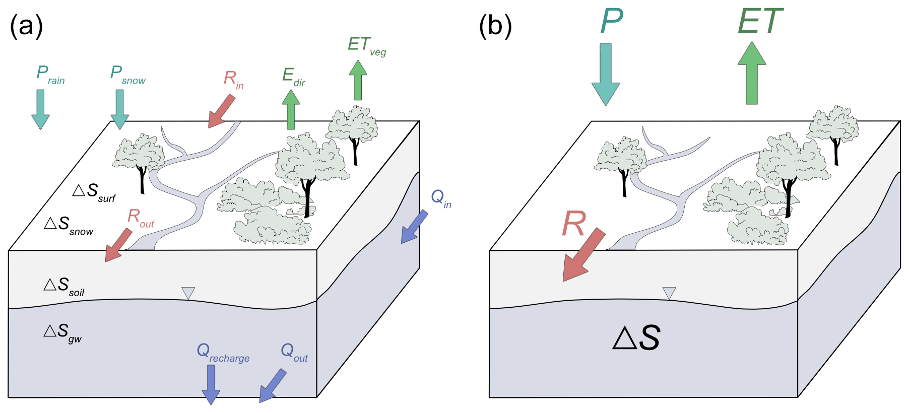
In Eq. (1), inflows to the watershed are precipitation in the form of rain or snow (Prain,Psnow), surface runoff entering the basin from upstream areas (Rin), or subsurface influx (Qin). Water may leave the watershed in the form of surface runoff (Rout), evapotranspiration from transpiration (ETveg) or evaporation from bare surfaces (Edir), or as groundwater flux to downstream basins (Qout) or deeper reservoirs (Qrecharge). These fluxes have a net impact on yield increases or decreases in sources of basin water storage, such as soil and groundwater reservoirs (ΔSsoil and ΔSgw), surface water ponding (ΔSsurf), or storage as snow water equivalent (ΔSsnow). Components in Eq. (1) are typically expressed as units of equivalent water height or volume per unit of time. This description of the water budget equation (Eq. 1) is illustrated in Fig. 1a, and it may be amended to incorporate other components particular to a watershed; these could include anthropogenic fluxes and storage like irrigation, dam storage or pumping, or they could be unique traits of the basin such as fractured flow, lacustrine groundwater discharge, or seawater intrusion. Equation (1) may also be simplified by lumping precipitation, evapotranspiration, and storage components and also by ignoring surface and subsurface inputs external to watershed divides, which, for large enough control volumes, will be negligible (Fig. 1b). The water balance may then be simply expressed as
for precipitation P, evapotranspiration ET, surface runoff R, and total change in all storage sources ΔS.
In this study, the complete water balance (Eq. 1, Fig. 1a) is modeled using ParFlow–CLM (Kollet and Maxwell, 2006; Maxwell and Miller, 2005), an integrated groundwater–surface water model which uses the mixed form of the Richards equation to simulate three-dimensional variably saturated flow. The Richards equation is given as
for specific storage Ss (L−1), relative saturation S (–), pressure head ψp (L), saturated hydraulic conductivity tensor Ks (LT−1), relative permeability kr (–), and porosity of the medium ϕ (–) at depth z (L) and time t (T). In Eq. (3), relative permeability varies with pressure head through time based on relationships established by van Genuchten (1980), and qs is a source–sink term (T−1). A free-surface overland-flow boundary condition for continuity of pressure and flux applies to the groundwater flux term across the land surface and subsurface interface. The kinematic wave approximation of the momentum equation is used to solve overland flow, which is a function of ponded depth given by Manning's equation:
where n is the Manning roughness coefficient () and ψ is the ponding depth (surface pressure head) (L). Note that the friction slope S0 (–) in Eq. (4) is used to approximate the bed slope (–) in the kinematic wave approximation.
ParFlow is coupled with the Common Land Model (CLM) (Dai et al., 2003), a land surface model which balances energy and calculates evapotranspiration at the land surface, in order to simulate the coupled water and energy budgets. CLM requires atmospheric conditions (precipitation, temperature, specific humidity, wind speed, and longwave and shortwave radiation) in order to provide hourly partitioning of net radiation into sensible, latent, and ground heat. Shown in Eq. (5), CLM calculates direct evaporation from the ground using the gradient between specific humidity at the ground surface qg (MM−1) and at a reference height qa (MM−1), along with air density ρa (ML−3), atmospheric resistance rd (TL−1), and a soil resistance term β (–).
To calculate actual transpiration, CLM adjusts potential transpiration by stomatal and aerodynamic resistance terms as follows.
Potential transpiration (Eq. 6) is a function of leaf and stem area index LAI and SAI (–), boundary layer resistance rb (TL−1), air density ρa (ML−3), and the gradient of specific humidity between foliage and canopy qf−qc (MM−1). Transpiration (Eq. 7) only occurs from the dry fraction of the canopy (Ld) and further depends on stomatal resistance rs (TL−1). In Eq. (7), the sunlit (sun) and shaded (sha) fractions of the dry canopy are separately defined with their own LAI and stomatal resistance values. Note that the leaf and stem area index and stomatal resistance terms are parameterized by plant functional types and defined per cell, without fractional vegetation, and for a single canopy layer. For a further explanation of ET calculations in ParFlow–CLM, see Jefferson et al. (2017).
2.2 PFCONUSv1 configuration, parameters, and inputs
The PFCONUSv1 model represents the first integrated groundwater–surface water model employed at the continental scale at hyper-resolution (1 km). A full description of the model configuration and inputs can be found in Maxwell et al. (2015) and Maxwell and Condon (2016), but a brief summary is given below.
Spanning roughly 6.3 million km2 at 1 km lateral grid spacing, the PFCONUSv1 model encompasses the majority of eight major river basins in the United States at high resolution, including the Ohio, Missouri, Arkansas, Mississippi, and Colorado River basins. The model is composed of 3442 cells in the x (east–west) direction and 1888 cells in the y direction (north–south). Its five vertical layers of variable thickness provide a cumulative vertical depth of 102 m. From the top, soil layers are 0.1, 0.3, 0.6, and 1 m, respectively. Topographic slopes were calculated using the Barnes et al. (2016) algorithm, applied to the HydroSHEDS (Hydrological data and maps SHuttle Elevation Derivatives at multiple Scales; Lehner et al., 2008) digital elevation model, to guarantee a connected drainage network. Vegetation classes for characterization of plant functional parameters were provided by the IGBP land cover classifications and the USGS land cover dataset. Distributed, heterogeneous soil parameters, including saturated hydraulic conductivity, porosity, and van Genuchten parameters, were assigned to spatial soil units described by the Soil Survey Geographic database (SSURGO). Geologic units for the bottom 100 m thick layer of the PFCONUSv1 model were developed from the Gleeson et al. (2011) national permeability map. Estimates from Gleeson et al. (2011) were adjusted using the e-folding relationship described in Fan et al. (2013), which accounts for topographic complexity, and variance in permeability was also reduced. No-flow boundary conditions were imposed at the bottom of the model domain (assuming impermeable bedrock) and on the sides. Note that with a model depth of just over 100 m, the model may more appropriately be considered a shallow aquifer storage model. Deeper ΔS contributions are not resolved, which may not represent deeper hydrologic flow paths of thick and expansive aquifers such as the Ogallala, the saturated thickness of which can exceed 300 m (McGuire et al., 2012); however, as Maxwell et al. (2015) explain, the current model thickness and vertical discretization are limited not by computational expense but by data availability, with a lack of detailed depth-to-bedrock and aquifer thickness estimates at meaningful resolution.
Initial conditions were provided by an intensive spin-up process. First, a steady-state ParFlow groundwater configuration was run continuously without CLM; this model was forced by an average surface recharge flux derived from Maurer et al. (2002) and run continuously until the difference between outflow and recharge rates was less than 3 % of total water storage change. A full description of this steady-state model and its performance can be found in Maxwell et al. (2015). Second, and using the initial condition provided by the steady-state model, a transient system was simulated with the fully coupled ParFlow–CLM for water year 1985, the most climatologically average water year within the past 30 years. As described in Maxwell and Condon (2016), atmospheric forcing was bilinearly interpolated from the North American Land Data Assimilation System Phase 2 (NLDAS-2) (Cosgrove, 2003; Xia et al., 2012a, b) For spin-up purposes, the transient simulation was run continuously for 4 years of repeated 1985 atmospheric forcing to provide an initial condition for the simulation in this study. Thus, the initial condition provided here represents pressure head, soil moisture, and surface energy balance conditions that would be present during the most climatologically average water year in recent history. Since the model does not incorporate anthropogenic abstractions in the form of pumping, injections, irrigation, or surface water diversions and dam storage, the initial conditions provided also represent a pre-development scenario.
For this study, PFCONUSv1 was run for modern-day water years using initial conditions provided by the transient spin-up process described above. The simulation here was run at hourly temporal resolution for water years 2003 through 2006. Atmospheric forcing originated from the 12 km NLDAS-2 product (Xia et al., 2012a, b); however, finer-resolution products were blended in where available and elevation effects were incorporated to produce higher-resolution, more physically realistic meteorological variables. Such products included the 4 km Stage IV and Stage II radar and gauge products and Level 2 shortwave radiation from the GOES Surface and Insolation Products (GSIP). These adjustments to the 12 km NLDAS data and the finer-resolution products are described, for example, in Pan et al. (2016) and include the following: gap-filling and daily rescaling procedure to ensure the Stage IV hourly data match daily totals from NLDAS-2; adjustments to timing for the GSIP Level 2 data based on solar angles; and elevation-dependent downscaling of 12 km NLDAS-2 products, such as hydrostatic effects for atmospheric pressure and lapse rates for specific humidity, air temperature, and longwave radiation. The final atmospheric variables were interpolated using bilinear interpolation to the 1 km PFCONUSv1 grid.
Table 1Products used to evaluate PFCONUSv1-simulated water balance component performance.

An important consideration when attempting high-resolution integrated models of this kind is of course the computational demand. ParFlow–CLM solves the globally implicit solutions to nonlinear and coupled equations in Eq. (3) through Eq. (7) with a Newton–Krylov parallel solver (Jones and Woodward, 2001); the associated significant computational challenge is tackled with a multigrid preconditioner and highly scaled parallel efficiency (Kollet et al., 2010; Reed M. Maxwell, 2013; Osei-Kuffuor et al., 2014). The simulations presented here were run on 3456 processors distributed to 72 and 48 units in the x and y directions, respectively, on the Cheyenne high-performance computing system managed by the National Center for Atmospheric Research (NCAR) Computational and Information Systems Lab. Required core hours for a single water year averaged over 300 000 core hours for this processor topology; however, the scaled parallel efficiency even at this decomposition is over 60 %. The hourly outputs generated over 11 TB of information per water year, while the required storage for the interpolated atmospheric forcing alone was over 3 TB per water year.
2.3 Datasets for comparison
Simulated runoff, evapotranspiration, and sources of storage change from the PFCONUSv1 model were compared against available point-scale measurements and coarse-resolution remote sensing products in order to identify locations of relatively better or worse performance, major sources of model bias, and regions most in need of improvement. Table 1 provides a summary of all data products compared to PFCONUSv1 outputs. It is important to note here that while we use absolute error metrics common to calibrated models developed specifically for prediction, calibration of the PFCONUSv1 model is not a goal of this study, nor is it feasible given the computational demands posed by such a highly parallelized platform. Rather, the intent is to evaluate the model's ability to demonstrate realistic behavior, to identify regions, times, and sources of uncertainty, and to prioritize areas of improvement for future model development.
2.3.1 Surface water runoff, R
Modeled surface water runoff (R in Eq. 2) was compared to daily observations at 2392 US Geological Survey (USGS) stream gauges containing observations over the simulation period (1 October 2002 through 30 September 2006) within the PFCONUSv1 domain (Table 1) (obtained from https://waterdata.usgs.gov/nwis/sw, last access: 2 February 2020). As discussed in the supplemental information for Maxwell and Condon (2016), the algorithm used for topographic processing resulted in spatial inconsistencies between the real and modeled stream network. USGS gauges were therefore mapped to the PFCONUSv1 grid using a combination of nearest-neighbor mapping and manual adjustments to ensure that all gauges lay on an appropriate ParFlow stream cell; for instance, a gauge comparison point that was incorrectly mapped upstream of a confluence may be moved to an appropriate location downstream. The large majority of mapped gauges were within 3 km of their “actual” location. As Maxwell and Condon (2016) explain, approximately 10 % of USGS gauges required more significant manual adjustments because of considerable discrepancies between the true stream network and that constructed for the model.
2.3.2 Evapotranspiration, ET
For evapotranspiration (ET in Eq. 2), three datasets are used to evaluate PFCONUSv1 results (Table 1). Observations from FLUXNET, an international network of meteorological towers that rely on the eddy covariance method to estimate evapotranspiration, were used to evaluate the temporal performance in ET. FLUXNET data were obtained from the FLUXNET 2015 online data portal (https://fluxnet.fluxdata.org/, last access: 6 February 2020), and the 30 sites used in this study are those that contain at least 1 water year of observations during the simulation period. PFCONUSv1 ET estimates were also compared to the MODIS evapotranspiration MOD16A2 monthly product provided by the University of Montana Numerical Terradynamic Simulation Group (NTSG) lab (http://files.ntsg.umt.edu/data/NTSG_Products/MOD16/, last access: 20 March 2020). The MODIS product, a NASA and EOS initiative to estimate global terrestrial evapotranspiration using satellite remote sensing data, uses a Penman–Monteith-based approach, stomatal resistance, and vegetation information to estimate evapotranspiration at an 8 d interval at 1 km resolution (Mu et al., 2007, 2011). MOD16A2 improves upon the original MOD16 ET algorithm by considering surface energy partitioning and atmospheric demand as well as land cover, leaf area index, and meteorological reanalysis products provided by NASA's Global Modeling and Assimilation Office (GMAO). Given the 8 d interval limitation and point-based uncertainties in ET of up to 40 %–60 % (Velpuri et al., 2013; Westerhoff, 2015), the monthly MOD16A2 product was spatially aggregated to HUC8 watersheds across the PFCONUSv1 domain with equal-area weighting. We also compare HUC8-aggregated monthly PFCONUSv1 evapotranspiration with estimates from the Operational Simplified Surface Energy Balance (SSEBop) algorithm (Senay et al., 2013). The SSEBop model is a relatively simple model using 1 km 8 d MODIS remotely sensed thermal imagery (land surface temperature and emissivity), combined with thermal index reference ET (Senay et al., 2013). Velpuri et al. (2013) evaluated MOD16A2 and SSEBop performance across the contiguous United States at point and basin scales, finding that SSEBop outperformed MOD16A2 in western arid basins. Note that for FLUXNET observations, ET (mm d−1) was derived from latent heat (W m−2) by scaling by the latent heat of vaporization λ (2.45 MJ kg−1) with the proportional relationship .
2.3.3 Storage, S
To evaluate PFCONUSv1 storage change (ΔS in Eq. 2), four products are used to compare to individual storage components, including total water storage, snow water storage, and soil water storage. Modeled snow water equivalent was compared to Snow Telemetry (SNOTEL) station data, a network maintained by the Natural Resources Conservation Service (NRCS). SNOTEL data were accessed from the NRCS online report generator 2.0 (http://wcc.sc.egov.usda.gov/reportGenerator/, last access: 28 February 2020). Of the available SNOTEL stations, 556 are within the PFCONUSv1 domain and have observations during the simulation period. These SNOTEL locations were compared to simulated snow water equivalent at their nearest-neighbor PFCONUSv1 grid cells. For soil water storage, soil moisture anomalies were derived from the active/passive satellite products from the ESA Programme on Global Monitoring of Essential Climate Variables (ECV) Soil Moisture Climate Change Initiative (CCI) project v04.5 (Gruber et al., 2019; https://www.esa-soilmoisture-cci.org/node/237, last access: 20 February 2020). This remote sensing product uses a combined estimate of soil moisture from four active and seven passive microwave sensors, providing soil storage at 0.25∘ resolution. ESACCI soil moisture estimates were compared to soil moisture in the top layer of PFCONUSv1, representing up to 0.1 m of depth.
PFCONUSv1 total water storage anomalies (an aggregate of all subsurface, snow water, and surface water storage components) were also compared to terrestrial water storage anomalies provided from remote sensing products from the Gravity Recovery and Climate Experiment (GRACE). The GRACE products are derived from slight fluctuations in Earth's gravity caused by changes in mass and measured by twin satellites launched in 2002; these gravity field changes over land may be attributable to terrestrial water storage change. GRACE solutions are provided by three processing centers: the NASA Jet Propulsion Laboratory (JPL), the GeoforschungsZentrum Potsdam (GFZ), and the Center for Space Research at University of Texas, Austin (CSR). In this study, PFCONUSv1 total water storage changes were compared to the Release-06 gravity field solutions (RL06) at 1∘, calculated using the spherical harmonic approach (Landerer and Swenson, 2012) with varying degrees and orders, spherical harmonic coefficients, and filtering processes. We also compare PFCONUSv1 to the mass concentration block (mascon) solutions provided by JPL at 0.5∘ and CSR at 0.25∘ (Save et al., 2016; Wiese et al., 2016), which eliminate much of the need for empirical post-processing and filtering required in the spherical harmonic solutions. The GRACE products listed above are hereafter referred to as JPL, GFZ, and CSR for the RL06 spherical harmonic solutions and JPLm and CSRm for the mascon solutions. For both the ESACCI soil moisture product and the GRACE total water storage anomalies, PFCONUSv1 estimates are aggregated to the coarse-resolution product by area-weighted mean prior to comparisons.
Finally, PFCONUSv1-calculated depths to water table are compared with water levels from 41 269 USGS groundwater wells across the continental United States; like streamflow, these data are freely available for download from the USGS National Water Information System (https://waterdata.usgs.gov/nwis/gw, last access: 23 March 2020). Of these wells, locations with more than 10 observations during the simulation timeframe and that met requirements for appropriate aquifer comparison (such as well depth, aquifer type, and anthropogenic influence) were used to calculate correlations with PFCONUSv1 time series; 2486 wells fit these criteria (see Table 1) and will be discussed further in Sect. 3. Note that in this study, we focus on the change in water storage over a given period of time rather than the total amount of water currently stored. Storage anomalies are presented as deviations through time from mean storage states; we also discuss the water storage amplitude, or peak-to-peak intra-annual storage change, for a given region as a proxy for seasonality. In the majority of the PFCONUSv1 domain, over this relatively brief simulation period, the variance in the intra-annual (seasonal) signal explains the majority of the variance in storage anomaly time series.
2.3.4 Atmospheric forcing
One important source of bias is that of atmospheric forcing; to evaluate the impact of meteorological performance on simulated water balance variables, we compare the interpolated NLDAS product to observed daily precipitation (N=9193) and observed averaged daily temperature (N=1678) at meteorological stations maintained by the Global Historical Climatology Network (GHCND) (Table 3.1) (data accessed via Climate Data Online portal, https://www.ncdc.noaa.gov/cdo-web/search, last access: 11 February 2020). Atmospheric forcing variables were also compared to observed data at SNOTEL and FLUXNET sites.
2.4 Performance metrics
Performance metrics for evaluating PFCONUSv1 include percent annual bias or total annual bias, Spearman rank correlation coefficient, and the ratio of root mean squared error to the standard deviation of observations (RSR). While these were not calculated for all validation datasets and the temporal resolution at which they were evaluated differed between datasets (e.g., daily, weekly, or monthly), they are each used at some point in our analysis, so we define them here.
As a measure of average magnitude accuracy with an optimal value of 0, percent bias is given by
where Si and Oi are simulated and observed values. Percent bias in PFCONUSv1 outputs was calculated using daily observations in Eq. (8) such that days during which observations were unavailable were excluded for both simulated and observed annual totals. Percent bias is an effective metric for evaluating long-term mean values, but it cannot be used to evaluate timing or shorter temporal events; further, if the model underpredicts and overpredicts with similar magnitudes, PBIAS can be deceivingly low.
For these reasons, we also calculate for each stream gauge Spearman's rank correlation coefficient, or Spearman's ρ, given by Eq. (9).
Unlike the coefficient of determination R2, which describes the degree of collinearity between the data, Spearman's ρ independently ranks the simulated and observed values, with di in Eq. (9) being the difference in ranks for a given value i, and n is the number of values in the series. Unlike other metrics describing temporal correlation, such as R2 or Nash–Sutcliffe efficiency, ρ is less restrictive; it does not assume linearity and instead tests for monotonic correlation. The optimal value for ρ is 1, and the cutoff for good performance is likely analogous to that of R2, which varies in the literature but is generally around 0.6.
A final performance metric, the RMSE–observation standard deviation ratio (RSR), is also provided. RSR is given by Eq. (10) and describes root mean squared error (RMSE) relative to the standard deviation of the observations.
In Eq. (10), is the mean of observations. While RSR is less widely used than PBIAS and ρ, its benefit lies in its normalization of the common error index statistic RMSE; the ratio describes error relative to natural variability in the true system such that an RSR of 1 suggests that the mean daily error is equal to 1 standard deviation of observed values and thus comparable to what we may expect from noise or intra-annual variability. An RSR value of 0 is optimal, while values under 0.5 (RMSE is less than half of the standard deviation of observations) are considered to be excellent (Moriasi et al., 2007).
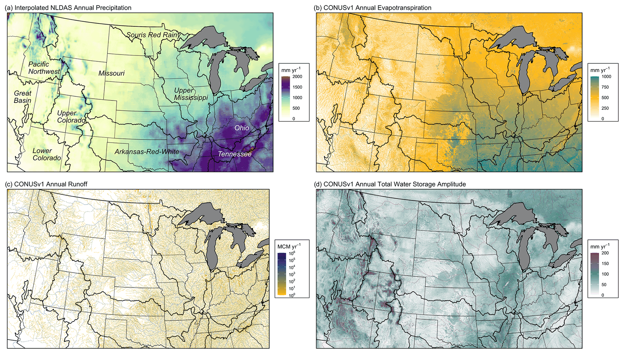
Figure 2Mean annual water balance components from PFCONUSv1 at 1 km resolution: (a) interpolated precipitation P from atmospheric forcing inputs, (b) simulated mean annual evapotranspiration (ET), (c) simulated mean annual runoff R, and (d) simulated mean annual total water storage ΔS amplitude (combined seasonality of snow water equivalent, groundwater, soil water, and surface water). Total water storage amplitude is the peak-to-peak seasonal storage anomaly rather than annual storage trend; seasonality (rather than inter-annual variability) explained the majority of the variance in total ΔS. Dotted lines are states, while thicker solid lines are major US river basin outlines, which are labeled in (a).
Together, performance metrics (Eq. 8 through Eq. 10) are quantitative indicators of model realism, representing a model's ability to capture long-term states (PBIAS) and timing (ρ), as well as its error relative to expected system variability (RSR). However, many other statistical criteria are popular (Waseem et al., 2017), and the target values used to indicate unacceptable, acceptable, or excellent performance can vary because criteria for evaluation necessarily depend upon model purpose (i.e., a regional surface water model that has been well calibrated for operational forecasting will represent spatiotemporal patterns of streamflow with higher accuracy than a continental-scale land surface model can plausibly achieve). Further, performance is expected to decrease with increasingly higher temporal resolution: for instance, criteria may be more lenient across all error metrics when moving from monthly to daily timescales at the watershed scale (Moriasi et al., 2015) as well as from seasonal to monthly timescales at the global scale (Krysanova et al., 2020). As a physically based, high-resolution (spatially and temporally), and uncalibrated continental-scale model, a primary purpose of the PFCONUS, and others like it (Gleeson et al., 2021), is to understand process interactions between groundwater, surface water, and ecohydrological fluxes. In this study, a PFCONUS-simulated water balance component in Eq. (2) is generally judged to be excellent for this purpose with the following measures: RSR < 0.6, ρ > 0.7, or |PBIAS| < 20 %. Locations that indicate unacceptable or poor performance are those with RSR < 1.2, |PBIAS| < 75 %, and ρ > 0.5. However, error metrics are reported with the primary goal of intercomparison across locations (interpretation of metrics should be paired with visual inspection of spatial patterns and time series provided) or, where discussed, relative to the performance of other continental-scale hydrologic or land surface models. Gleeson et al. (2021) caution against the use of model evaluation to indicate a “finished” product and instead recommend open-ended evaluation and model improvement. Metrics (Eq. 8 through Eq. 10) are therefore used to identify where future development of PFCONUS can be focused to improve upon timing, volume, and variability of fluxes. Performance metrics reported in this study are also supplemented by plots of probability of exceedance or non-exceedance where appropriate (see Figs. S1 through S8 in the Supplement), which should help regional-scale modelers identify relative performance of major basins at various thresholds. Since there are many other commonly used performance metrics particular to streamflow, we also report Nash–Sutcliffe efficiency and Kling–Gupta efficiency for simulated flows at USGS gauges (Fig. S9 in the Supplement) (Gupta et al., 2009).
By providing detailed partitioning of the water and energy budgets at high spatial and temporal resolution and at continental spatial extent, the PFCONUSv1 ParFlow–CLM model offers an unprecedented opportunity to study large-scale nonlinear relationships and to provide hydrologic process estimates at locations remote from observation networks. The 2003–2006 water year simulations in this study estimate hourly pressure head and saturation at each of the approximately 31.5 million 1 km three-dimensional model cells; the simulations also provide evapotranspiration and energy balance estimates at each of the 6.3 million land surface grid cells. Figure 2 shows the PFCONUSv1 model extent, mean annual precipitation from interpolated atmospheric forcing, and mean annual simulated components of Eq. (2). Below, these water balance components, their performance, and their relative bias sources are discussed in detail. Note that different performance metrics were discussed for model components based on their temporal and spatial coverage, continuity, resolution, and uncertainty. For instance, the sheer amount of temporal and spatial coverage provided by the USGS stream gauge network allowed for several different error metrics to evaluate long-term behavior, hydrograph shape, and flashiness. Comparisons of model results with remote sensing products and well observations were more limited by higher uncertainty and lower temporal and spatial resolution and continuity, but they were still valuable in identifying regions for model improvement and analyzing error propagation between water balance components.
3.1 Runoff, R
The ability to accurately simulate overland flow at the major basin or continental scale and above has for several years been a topic of much interest in the hydrologic community. Continental or global streamflow estimates could be coupled to general circulation models to provide predictions of surface water resource vulnerability to climate change (e.g., Koirala et al., 2014); large-scale runoff models could additionally provide flood forecasts to regions lacking developed surface water monitoring networks (Kauffeldt et al., 2016). While integrated groundwater–surface water modeling is computationally demanding, results from PFCONUSv1 represent a rare opportunity to evaluate streamflow performance (1) because the integrated system platform resolves shallow aquifer, vadose zone, and surface water transfer, and (2) streams form naturally as surface water is routed by topography without requiring pre-defined stream reaches.
PFCONUSv1 streamflow R was evaluated against 2392 USGS stream gauges which are well distributed across the United States. We analyze model performance using percent bias, Spearman rank correlation, and RSR. However, Gleeson et al. (2021) suggest that while the use of error metrics and direct comparison of observations with simulated values are valuable for evaluation, they should be supplemented with hydrologically meaningful diagnostic signatures to better understand system dynamics. Further, PBIAS can be sensitive to precipitation provided by the interpolated NLDAS atmospheric forcing product. Since P is an input to the PFCONUSv1 rather than a model result, runoff ratio () was also calculated to extract model performance independent of precipitation bias and to better represent a diagnostic measurement of watershed response to rainfall. RR measures the amount of precipitation partitioned to runoff, with lower RR values generally indicating a greater portion of precipitation lost to infiltration or evapotranspiration. “True” runoff ratios were estimated by first identifying all GHCND precipitation gauges upstream of a USGS stream gauge. The mean annual precipitation was then calculated and applied over the drainage area defined by the Geospatial Attributes of Gages for Evaluating Streamflow (GAGES-II) dataset (Falcone, 2002). RR is equal to the ratio of total USGS gauge flow to GHCND precipitation. A similar process was done for simulated RR using NLDAS-interpolated precipitation, simulated flow at the gauge cell, and model drainage area from the input digital elevation model derived from HydroSHEDS. Note that while the interpolated NLDAS precipitation, unlike the GHCND gauge network, is continuous in space, only modeled cells which matched the nearest-neighbor GHCND gauge network were used to estimate upstream precipitation in order to create as controlled a comparison as possible. Runoff ratios were not calculated for USGS stream gauges with fewer than three upstream GHCND precipitation gauges.
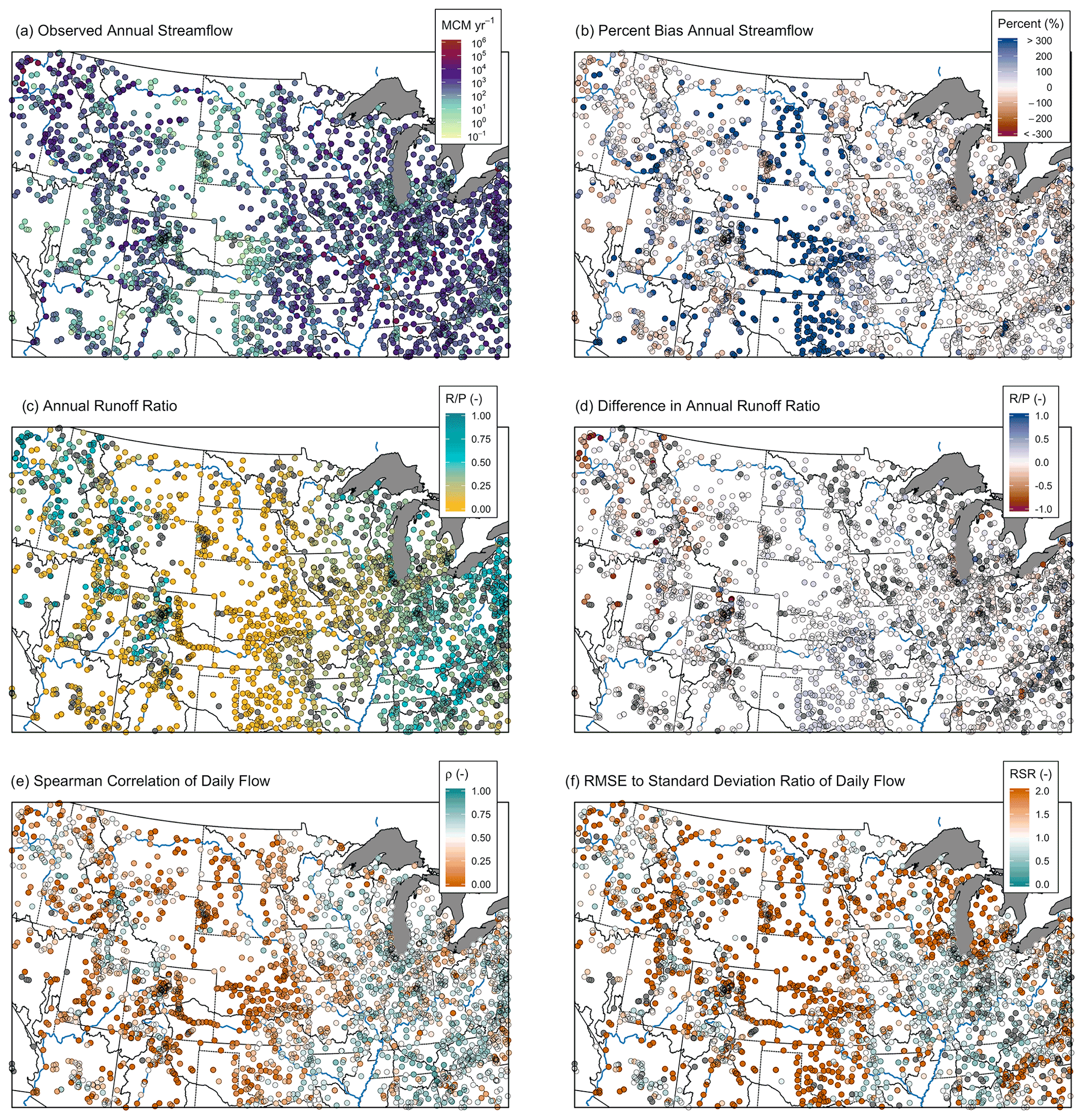
Figure 3(a) Observed annual streamflow R from the USGS gauge network, (b) PBIAS for simulated PFCONUSv1 streamflow, (c) runoff ratio calculated from USGS stream gauges and GHCND precipitation gauges, (d) simulated minus observed runoff ratio, (e) ρ of simulated daily flows, and (f) RSR of simulated daily flows.
Observed total annual flow during the simulation period is shown in Fig. 3a; annual streamflow varies by several orders of magnitude across US major basins, with higher flows in the east and the Pacific Northwest and the lowest flows in the Great Plains. Runoff ratios are generally highest in the east; the majority of the arid west exhibits RR of less than 0.1, with the exception of topographically complex regions and headwater watersheds of the Rocky Mountains (Fig. 3c).
PFCONUSv1 reproduces point-scale annual flows across the United States with a median annual PBIAS of 7.7 % and with 25th and 75th percentiles of −26.2 % and 77.4 %, respectively (Fig. 3b). Shown in Fig. 3e and f, the 25th, 50th, and 75th percentiles for daily Spearman's ρ are 0.42, 0.65, and 0.76, while the same for RSR are 0.86, 1.2, and 2.5. The median PFCONUSv1 minus USGS difference in RR is 0.016 (Fig. 3d), which corresponds to a mean percent bias in runoff ratio of 8.3 %. The PFCONUSv1 model simulates observed streamflow with RSR < 0.6, ρ > 0.7, and |PBIAS| < 20 % at 54 gauges (approximately 2 % of available sites). An additional 97 locations (4 % of gauges) exhibit RSR < 0.7, ρ > 0.65, and |PBIAS| < 30 %. An additional 382 locations (15.7 % of gauges) show RSR < 1, ρ > 0.6, and |PBIAS| < 50 %. And, finally, an additional 268 gauges (11 % of gauges) show RSR < 1.2, ρ > 0.5, and |PBIAS| < 75 %. As has been shown in previous literature (Waseem et al., 2017), different performance metrics do not always indicate the same closeness of fit: while 2099 gauges (86 % of the dataset) show either RSR < 1.2, |PBIAS| < 75 %, or ρ > 0.5, only 801 gauges (34 % of all gauges) fit all those criteria.
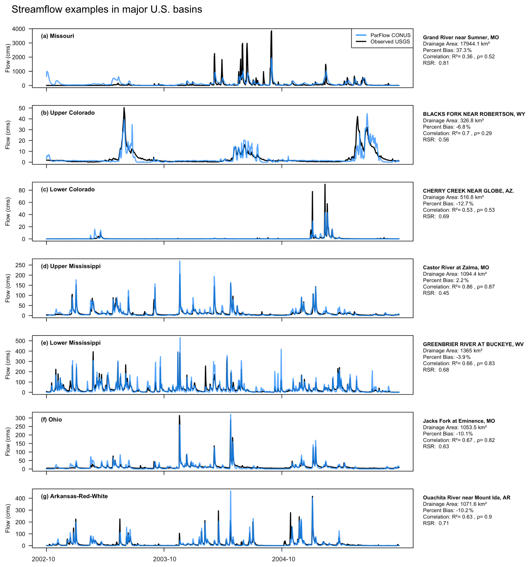
Figure 4Time series of PFCONUSv1-modeled and USGS-observed streamflow time series at representative gauge locations for each major basin.
Streamflow performance varies widely across major basins. For instance, median PBIAS, ρ, and RSR for the Ohio River Basin are −7.8 %, 0.79, and 0.84, respectively, and the median of simulated RR values is within 6 % of the median estimate of RR = 0.42 from observations. Simulated flows in the Tennessee River Basin also appropriately simulate observed flows: mean PBIAS, ρ, and RSR are −11.9 %, 0.69, and 0.89, respectively; 60 % of the gauges in the basin perform with RSR < 1.2, ρ > 0.5, and |PBIAS| < 75 %, and observed and simulated mean RR values are 0.49 and 0.53, respectively, for a percent bias in RR of 9 %. Conversely, the majority of the upper Missouri River Basin shows weak timing performance (median ρ of 0.49) and higher overall bias: the median PBIAS for Missouri is 65 % and median RSR is 2.2, indicating that the majority of Missouri gauges exhibit daily RMSE that is twice the volume of expected daily variability. The Great Plains region is certainly the region with the worst streamflow performance: PFCONUSv1 percent bias in the majority of these gauges is greater than 300 %, and in some cases, simulated flow is greater than 10 times the volume observed. While the mean difference in runoff ratio in this region is only 0.04, this is on average 4 times larger than RR estimated from observations. Results in Fig. 3 therefore suggest that in the arid Great Plains region, a very small change in runoff ratio can result in dramatic error in streamflow bias, and the PFCONUSv1 struggles to capture low flows in this region. There is evidence that continental-scale hydrologic models commonly share this struggle to capture streamflow dynamics in the Great Plains region. The first phase of the Continental Hydrologic Intercomparison Project has shown that a NOAA US National Water Model configuration of WRF-Hydro shares the same streamflow performance category (poor hydrograph shape and/or timing and high bias) as PFCONUSv1, run for the single water year 1985, at many gauges in the Great Plains region (Tijerina et al., 2021). While the intercomparison project is in its infancy and this comparison was primarily proof-of-concept, such results may stress the importance of representing groundwater abstractions and irrigation over the Ogallala in continental-scale hydrologic models.
Note that in Fig. 3, no filtering was done for these metrics in order to eliminate gauges with incorrect drainage area from topographic processing discrepancies, nor have we removed sites proximate to dams, influenced by nearby pumping or irrigation, or affected by bias in atmospheric forcing. As an example of PFCONUSv1 performance in ideal conditions, we show in Fig. 4 selected examples of individual gauge comparisons for each major basin in the PFCONUSv1 domain. Gauges chosen for Fig. 4 were those that tended to be minimally impacted by bias from anthropogenic effects or by errors in basin delineation by topographic processing. Such gauge attributes were determined based on geospatial stream properties obtained from the Geospatial Attributes of Gages for Evaluating Streamflow (Gages-II) dataset (Falcone, 2002), as well as the National Hydrography Dataset (see the supplemental information in Maxwell and Condon, 2016, for a detailed description of geospatial stream gauge attributes). Streamflow time series examples in Fig. 4 include gauges with the following properties: (1) represented greater than 300 km2 of upstream drainage area, (2) PFCONUSv1 drainage area differed from actual drainage area by less than 20 %, (3) total dam storage was less than 3 % of total annual flow for the closest upstream dam, (4) total withdrawals for the previous 5 years were less than 3 % of total annual flow, (5) total irrigated area in 2002 constituted no more than 15 % of the total drainage area, and (6) upstream area Spearman's ρ for precipitation performance must be greater than 0.5. The examples in Fig. 4 therefore represent naturalized gauges with minimal bias in a priori inputs, low anthropogenic impact, and good performance potential. We also compared domain-wide PFCONUSv1 performance at reference gauges identified by Maxwell et al. (2015) (locations with the least human influence and best representing “natural” ecohydrologic conditions) with non-reference gauges. As a whole, PFCONUSv1 performed better at reference locations regardless of the error metric used (Fig. S1). However, the difference in performance between reference and non-reference locations varies considerably between basins (Figs. S4 and S5). The Pacific Northwest, Missouri, Lower Colorado, and Arkansas–Red–White basins exhibit much greater performance at reference gauges across all error metrics, while other basins show mixed signals or poorer performance at reference gauges (Figs. S1 and S2), indicating sources of bias other than anthropogenic effects.

Figure 5(a) Cumulative annual ET observed at 30 FLUXNET sites across the contiguous United States, (b) percent bias of PFCONUSv1 daily simulated ET at FLUXNET locations, (c) Spearman ρ of PFCONUSv1 daily simulated ET at FLUXNET locations, (d) RSR of PFCONUSv1 simulated daily ET, and (e–g) examples of observed and simulated daily ET at three FLUXNET sites with complete observation periods during the simulation timeframe.
3.2 Evapotranspiration, ET
Evapotranspiration is a major component of the water balance, accounting for roughly 60 % partitioning of land precipitation into the atmosphere annually (Oki and Kanae, 2006); however, it is also widely considered to be an incredibly difficult value to constrain (Senay et al., 2013; Velpuri et al., 2013; Xu and Singh, 2005) and is often estimated simply as the residual of other components of the water balance. Unlike streamflow and precipitation, direct point measurement methodologies are limited, costly, and difficult to maintain. Direct estimates can be inferred from sap flux measurements; lysimeters, which weigh plant and soil mass to track temporal fluctuations in water storage; or chemical tracers, such as deuterium (Wilson et al., 2001). Currently, the method which likely provides the most defensible direct measurements of ET is the eddy flux or eddy correlation method. Eddy flux towers relate observed turbulent heat fluxes at the surface (latent and sensible heat) to the covariance between instantaneous fluctuations of vertical wind speed, humidity, and temperature (Baldocchi, 2003; Swinbank, 1951). The PFCONUSv1-simulated daily ET was compared to observations from 30 eddy covariance towers managed by the FLUXNET mission. Locations of these sites and their relative performance are shown in Fig. 5, along with time series examples from three FLUXNET sites with complete observations during the entire observation period.
Results in Fig. 5 demonstrate the ability of the PFCONUSv1 model to simulate daily and seasonal ET across difference climatic zones. The mean 25th, 50th, and 75th percentiles for PFCONUSv1-simulated daily ET PBIAS are 3 %, 26 %, and 55 %, respectively. Given that remote sensing estimates regularly exhibit uncertainty of 50 %–60 % for point-scale ET estimates, or > 20 % uncertainty in ET at the basin scale (Velpuri et al., 2013), PFCONUSv1 ET results are promising, especially for an uncalibrated model. For daily time series, 25th, 50th, and 75th percentiles are 0.6, 0.72, and 0.81 for ρ and 0.69, 0.92, and 1.33 for RSR, respectively. Because the metric is an indicator of monotonic agreement, the high overall Spearman's ρ values are particularly telling because ρ is sensitive not only to seasonal trends which dominate the time series variance but also the influential day-to-day (sub-seasonal) noise. Out of 30 FLUXNET sites with observations during the simulation time period, the PFCONUSv1 model performs with RSR < 1.2, |PBIAS| < 75 %, or ρ > 0.5 at 19 locations (63 % of locations); at 29 out of 30 sites, the PFCONUSv1-simulated ET fits one of these criteria.
The spatial discontinuity of FLUXNET certainly limits ET performance evaluation across the remaining PFCONUSv1 model domain. Eddy covariance ET estimates are applicable within the fetch of the prevailing winds, which is generally on the order of ∼ 1 km radius surrounding towers (Wilson et al., 2001), and statistical interpolation is generally not recommended without considerable parameterization of atmospheric and vegetative conditions to inform upscaling (Jung et al., 2009).
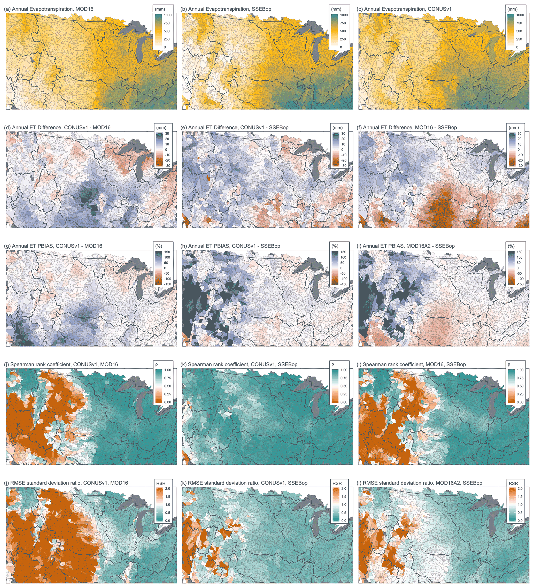
Figure 6PFCONUSv1 ET estimates compared to results from MODIS remote sensing and thermal imaging algorithms. (a–c) Annual cumulative ET across HUC8 watersheds, (d–f) differences in annual ET, (g–i) PBIAS of monthly ET, (j–l) Spearman's ρ of monthly ET, and (m–o) RSR of monthly ET for PFCONUSv1 and MODIS products (MOD16A2 and SSEBop algorithms).
To evaluate performance at larger spatial scales, the PFCONUSv1 model has also been compared to the MOD16A2 and SSEBop algorithms for MODIS thermal imagery processing. These data, along with PFCONUSv1, have been aggregated to HUC8 spatial scale and monthly temporal resolution to help reduce uncertainty associated with cloud cover in the 8 d product. Cumulative annual evapotranspiration for MOD16A2, SSEBop, and PFCONUSv1 are shown in Fig. 6a–c. Both MOD16A2 and SSEBop algorithms should be considered evapotranspiration modeling techniques produced from remote sensing observations rather than observations themselves. However, regions where PFCONUSv1 comparisons to the MOD16A2 and SSEBop agree establish greater confidence in the model's bias or timing of ET estimates. We have therefore used PBIAS, ρ, and RSR error metrics, with PFCONUSv1 monthly ET observations as simulated and MODIS datasets as observed values. Multiple studies to date have compared MOD16A2 and SSEBop performance over a range of geophysical characteristics, vegetative types, and aridity indices by comparing to Penman–Monteith-based estimates (Knipper et al., 2016), lysimetric observations (Senay et al., 2014), FLUXNET observations or upscaled information from FLUXNET sites, and vegetative indices (Senay et al., 2013; Velpuri et al., 2013), with results showing good general agreement and within ∼ 50 % error for annual ET totals at point observations. Despite its considerably more simplistic approach for estimating ET from MODIS thermal land imaging, SSEBop performs nearly as well as or, in the case of the western US, better than MOD16A2 (Velpuri et al., 2013). Therefore, we also show MOD16A2 performance relative to SSEBop for reference (Fig. 6c, f, i, l, and o), where Oi observations are MOD16A2 and Si observations are MOD16A2 monthly ET (Eqs. 8 and 10).
PFCONUSv1 shows similar overall agreement with MOD16A2 and SSEBop algorithms in annual ET, with differences within ± 30 mm across the domain. All products provide similar spatial signatures of ET, with overall higher ET in the southwest and the lowest ET in the Great Basin and Colorado River basins. PFCONUSv1 estimates tend to agree more with SSEBop with regards to timing and residual variation, and they are more similar to MOD16A2 with regards to PBIAS (particularly in the western United States) (Fig. 6). The 50th percentiles for PFCONUSv1 PBIAS against MOD16A2 and SSEBop are 7.5 % and 8 %, respectively; 25th and 75th percentiles of PBIAS are −4.4 % and 24 % for MOD16A2 and −4.4 % and 35 % for SSEBop. In several regions, PFCONUSv1 shows similar comparisons with both MODIS products. For instance, in the Upper Mississippi, both products suggest that PFCONUSv1 overpredicts ET in the north and underpredicts in the south, and both products suggest PFCONUSv1 underpredicts ET in the Rocky Mountain headwaters and across most of the Ohio River Basin (Fig. 6d and e). The approximately 30 % underestimation of ET in the CO headwaters further agrees with the PFCONUSv1 performance relative to FLUXNET observations at the Niwot Ridge site in Colorado. However, most of the Missouri and the Arkansas–Red–White basins show opposite behavior between PFCONUSv1-MOD16A2 and PFCONUSv1-SSEBop comparisons; in these regions, we can be less certain of model bias as described by remote sensing of ET. Broadly, across the western US, PFCONUSv1 shows better agreement with MOD16A2 with regards to ET magnitude (PBIAS) because SSEBop estimates negligible ET in the Basin and Range region (Fig. 6e); however, PFCONUSv1 shows dramatically better performance relative to SSEBop in terms of Spearman's ρ and RSR (Fig. 6g and h). The 25th, 50th, and 75th percentiles of ρ are 0.38, 0.85, and 0.92 for monthly PFCONUSv1 compared to MOD16A2; the quantiles for PFCONUSv1 compared to SSEBop are 0.85, 0.91, and 0.93. Similarly, 25th, 50th, and 75th percentiles of RSR are 0.41, 0.85, and 2.2 for performance relative to MOD16A2 and 0.38, 0.47, and 0.62 for performance relative to SSEBop.
Despite differences between PFCONUSv1 comparisons to the two MODIS algorithms, results shown in Fig. 6 suggest that PFCONUSv1 appropriately estimates the magnitude and temporal progression of ET compared to the performance of other LSMs. In a study comparing LSM-based recharge estimates in the western United States, Niraula et al. (2017) showed that the LSMs Mosaic, VIC, and Noah simulated spatially distributed ET with 0.87, 0.77, and 0.75 Pearson's correlation relative to MODIS. Pearson's correlations between PFCONUSv1 and MOD16A2, and between PFCONUSv1 and SSEBop, are 0.9 and 0.95, respectively, which motivates future comparisons of PFCONUSv1 performance relative to other LSMs. However, it is important to again note that MODIS ET estimates are themselves models, and as such they are susceptible to epistemic errors in input data (e.g., inaccuracies in leaf area index or other parameterizations), measurement and remote sensing errors (e.g., cloud cover), and other uncertainties.
3.3 Storage, S
Terrestrial water storage represents all components of the water balance stored on and below the Earth's surface. As such, total storage S is an aggregate of water stored on land in surface water bodies or in the canopy, as well as snow water equivalent, soil moisture in the vadose zone, and shallow or deep saturated aquifer storage. Estimates of overall S could simply involve measuring and combining individual components, but these calculations (1) require highly developed monitoring networks and an impressive amount of in situ observations and (2) can have large margins of error if not all of the assorted hydrological stores are accurately resolved (Troch et al., 2007). The most common method for S estimation calculates storage as a remainder of other water balance terms: P, ET, and R in Eq. (2), (e.g., Rodell et al., 2011; Tang et al., 2010).
Recent advances in remote sensing have granted hydrologists an estimate of changes to total S, without partitioning out storage sources, by measuring fluctuations of Earth's gravity fields as a proxy for mass change. Since water represents the greatest fluctuation of terrestrial mass, gravity anomalies can be translated to variability in S. The newly available GRACE twin satellite mission provides approximately monthly values of total water storage at the global scale and at coarse (> 105 km2) resolution (e.g., Strassberg et al., 2009). Storage anomaly estimates are based on K-band microwave measurements of the distance between the two low-flying satellites, which varies as a function of gravity field fluctuations (as well as atmospheric, oceanic, and solid Earth tides, which must be corrected to resolve the global water budget; Dahle et al., 2019).
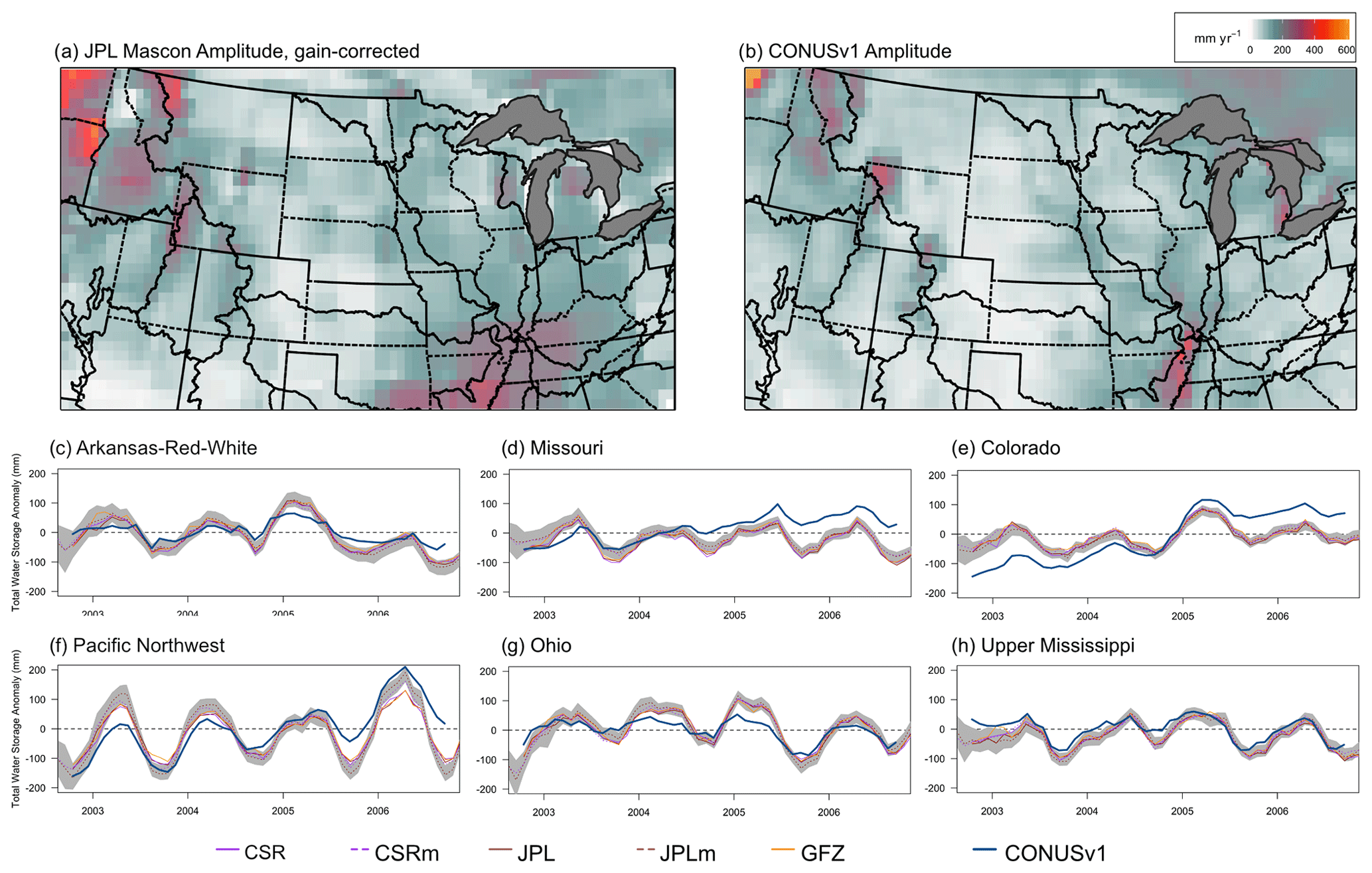
Figure 7Summary of GRACE and PFCONUSv1 comparisons. Seasonal storage amplitude for (a) the JPL mascon solution and (b) PFCONUSv1 total water storage, with darker red areas indicating a high degree of seasonality and white areas indicating no sub-annual storage fluctuation. (c–h) Time series of total water storage anomalies for five GRACE products and for PFCONUSv1 across complete major basins in the PFCONUSv1 domain. Shaded regions indicate uncertainty in the JPLm product based on leakage and measurement error.
The PFCONUSv1 total water storage anomalies (calculated as a sum of all simulated surface and subsurface hydrologic stores) were compared to five monthly gravity field solutions: the RL06 spherical harmonic solutions provided by JPL, GFZ, and CSR, as well as the mascon solutions JPLm and CSRm. Figure 7 shows seasonal storage amplitude in space and basin-aggregate storage change through time by comparing PFCONUSv1 and GRACE solutions for six major river basins. Some basins have been left out due to incompleteness in the model domain or due to size: the basis function for GRACE solutions is generally on the order of 300 000 km2 such that storage anomaly estimates for smaller basins (e.g., the Tennessee River Basin) are not well resolved.
Seasonal storage amplitude represents the average peak-to-peak storage gain or loss over the course of a water year, and it is therefore a depiction of seasonality or intra-annual S signal. The GRACE solution shown in Fig. 7 is the JPL mascon solution provided at 0.5∘ resolution, and amplitude for other GRACE products shows similar spatial signals; however, note that mascon solutions are calculated given a 3∘ equal-area basis function and subsequently downscaled using forward modeling techniques to account for leakage errors (Wiese et al., 2016). GRACE mascons are not independent of each other, and uncertainty increases dramatically with decreasing basin size. However, qualitative comparisons between GRACE and PFCONUSv1 amplitude indicate several regions of agreement for high or low seasonality. Topographic highs in the Rocky Mountains, where the snow water equivalent signal likely dominates overall storage variance and is entirely seasonally dependent, show high amplitude for both PFCONUSv1 and GRACE (Fig. 7a and b). The Upper and Lower Colorado River basins, in particular, show very similar spatial patterns for overall amplitude. Another area of agreement is the comparably high amplitude in the Lower Mississippi River basin. In both GRACE and PFCONUSv1, the Arkansas–Red–White region sees higher seasonality of total water storage in the east and lower in the west; the locations of highest amplitude for both GRACE and our model lie in the Pacific Northwest region. However, broadly speaking the PFCONUSv1 amplitude is lower than GRACE for the majority of the domain and particularly in the east. Other continental- or global-scale land surface models have also underpredicted seasonal storage amplitude across global river basins relative to GRACE; for example, the WaterGAP (Water Global Assessment and Prognosis) hydrologic model consistently underpredicted amplitude for most of the global land area (Döll et al., 2014), and a validation of four LSMs and global hydrologic models found that the numerical models reproduced GRACE storage signals only to a very limited degree (Zhang et al., 2017). However, LSM tendency for GRACE mismatch is likely attributed to insufficient groundwater representation, which is not as likely to be the cause for PFCONUSv1 and GRACE disparities.
Temporal progression of storage was calculated with the area-weighted mean of the Colorado, Arkansas, Ohio, Missouri, and Upper Mississippi River basins (Fig. 7c–h). Uncertainty (shaded regions) shown indicates the leakage error associated with downscaling 3∘ basis functions to 0.5∘ solutions for the JPL mascon product. We show only the JPLm uncertainty, simply because uncertainty estimates for the RL06 products were not yet available at the time of this analysis. The CSR mascon product is suggested to have an error of approximately 2 cm that is more or less constant through time and space.
The PFCONUSv1 model shows good agreement in the timing storage anomalies for most basins, with Spearman's ρ rank correlation ranging from 0.43 to 0.94 relative to the mean of all GRACE solutions: individual ρ values for major basins are 0.43 (Missouri), 0.63 (Upper Colorado), 0.76 (Pacific Northwest), 0.79 (Great Basin), 0.81 (Lower Colorado), 0.86 (Upper Mississippi), 0.88 (Ohio), and 0.93 (Arkansas–Red–White). However, correlation is not necessarily the best predictor of adequate model performance; for instance, the Upper Mississippi has the third-highest ρ value out of six major basins, but more than 80 % of the total anomaly time series lies within the uncertainty bars provided for the JPLm product. Further, several discrepancies exist between PFCONUSv1 and GRACE trends and amplitude. For example, despite its monotonic agreement with GRACE storage amplitude for the Ohio River Basin, the PFCONUSv1 model simulates a seasonal storage amplitude that is, on average, more than 30 % lower than what GRACE observes. The Upper Colorado River basin captures seasonal timing, but the overall storage gain over the simulation period is roughly 3 times that of what GRACE observes.
Differences between the PFCONUSv1 and GRACE storage water anomaly estimates can come from various sources: (1) model error and uncertainty in PFCONUSv1 model parameters and configuration, error and uncertainty associated with GRACE measurement error, or error associated with the intensive post-processing and filtering on the raw spherical harmonic GRACE solutions; (2) hydrologic stores unaccounted for in the PFCONUSv1 model, such as deep (> 100 m) aquifer storage; or (3) anthropogenic impacts, particularly from groundwater withdrawals from municipal and agricultural aquifer depletions (Chen et al., 2016).
3.4 Storage partitioning: Sgw, Ssoil, and Ssnow
Total water storage anomalies were also validated based on their partitioned components: ΔSgw, ΔSsoil, and ΔSsnow. First, PFCONUSv1 water table depth (WTD) was compared to USGS well observations across the United States in Sect. 3.4.1. As discussed below, WTD does not necessarily translate to ΔSgw, but it is still a very informative hydrologic state. PFCONUSv1 soil moisture was compared to a combined active/passive remote sensing product in Sect. 3.4.2, and PFCONUSv1 snow water equivalent was compared to snow telemetry measurements in Sect. 3.4.3.
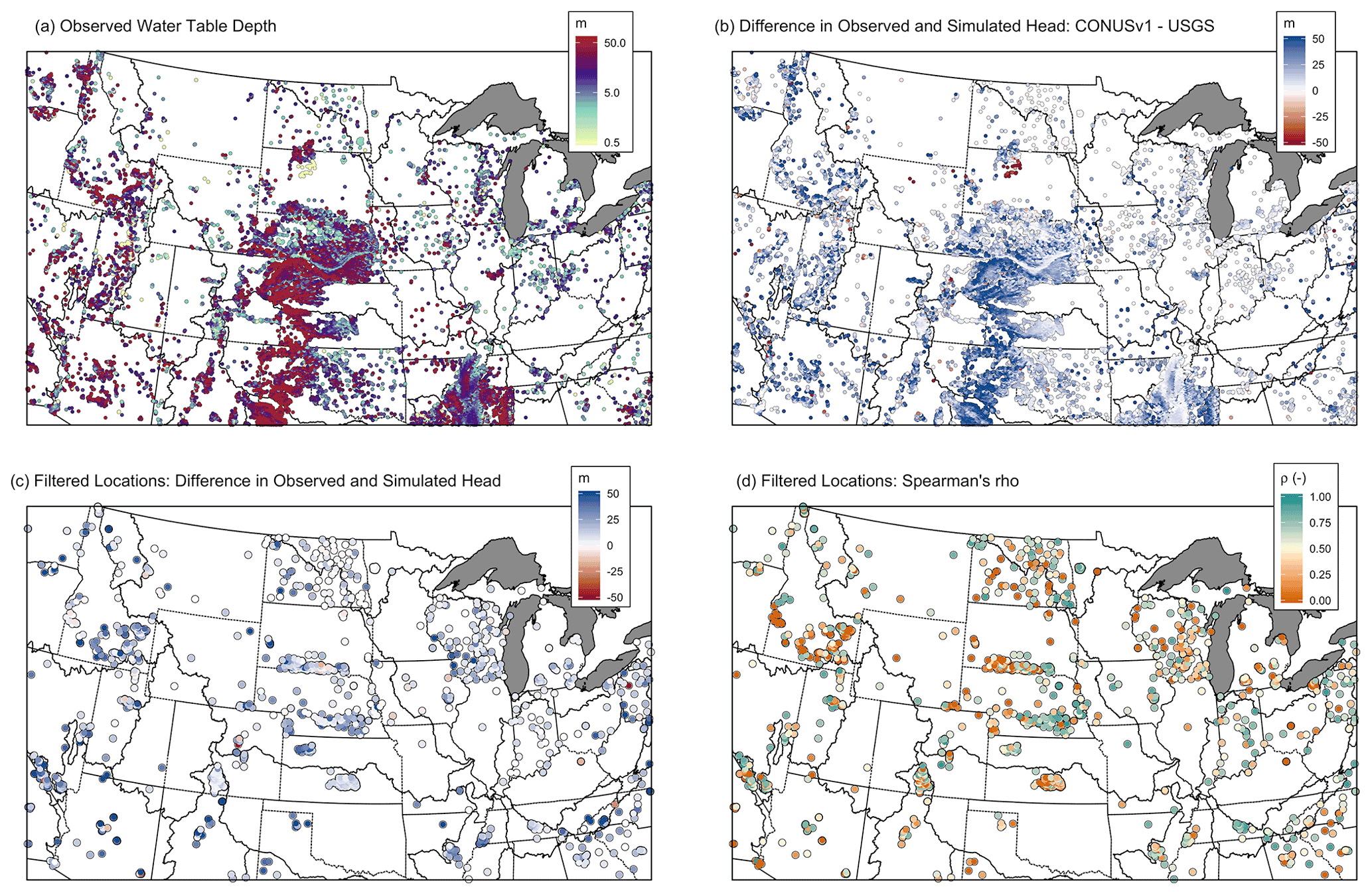
Figure 8(a) Observed water table depth (N = 41 269), (b) difference in observed and PFCONUSv1-simulated WTD, (c) difference in observed and PFCONUSv1-simulated WTD at filtered locations (N=2486), and (d) Spearman ρ values at filtered locations using at least 10 instantaneous (daily) observations.
3.4.1 Water table depth
Figure 8 shows observed WTD across the model domain, as well as difference in observed and modeled heads and correlation for available locations. As a caveat to the results shown in Fig. 8, while WTD is a visibly appealing metric for modeled groundwater performance, it alone is not translatable to total storage Sgw or for storage change ΔSgw for several reasons. First, without information regarding aquifer storativity or in the absence of pumping tests, change in water table depth does not equate to total water storage fluctuation in an aquifer of uncertain depth and hydraulic characteristics. Second, water flow is governed by hydraulic head rather than water table depth; therefore, a bias in WTD of tens of meters within a continental model that spans thousands of meters of hydraulic head does not necessarily speak to the model's ability to laterally move water through the saturated subsurface. Finally, perched and confined aquifer systems can completely disconnect anomalies in total subsurface hydrologic stores and measurable WTD fluctuations. However, WTD does indicate vadose-zone-saturated zone connectivity, and for unconfined aquifers it is a good indicator for loss or gain in aquifer storage, so we briefly compare observed and simulated WTDs here.
Observed WTD from over 41 000 aquifers across the contiguous United States spans multiple orders of magnitude and is shown in Fig. 8. The PFCONUSv1 model demonstrates a fairly consistent shallow WTD bias across the domain, with “hot spots” of over 50 m depth difference in the southern reaches of the Ogallala aquifer, in the southern Pacific Northwest region, and in the Lower Colorado River basin. However, many of these wells represent locations impacted by extractions (wells are preferentially drilled in regions prioritizing municipal or agricultural groundwater resources), wells tapping confined aquifers, or WTDs that simply cannot be captured by a shallow aquifer model of 102 m depth. In a 1985 transient simulation of PFCONUSv1, Maxwell and Condon (2016, supplemental information) found that while no strong connection exists between water table depth bias and the model's geologic properties, WTD bias was aquifer-dependent, with the greatest positive WTD biases occurring in the High Plains aquifer, which has experienced depletions in the last several decades.
Further, WTD is only informative as an indicator of positive or negative ΔSgw if multiple observations are provided through time. Therefore, the available USGS wells have been filtered by excluding (1) locations where the observed minimum WTD was greater than 60 m (PFCONUSv1 estimates pressure at cell centers, with the center of the deepest layer at 52 m), (2) locations providing fewer than 10 observations during the simulation timeframe, (3) locations flagged by the USGS as a confined or mixed aquifer system (aquifer type code aqfr_type_cd in the Groundwater Levels for the Nation dataset provided by USGS NWIS, https://waterdata.usgs.gov/nwis/gwlevels/, last access: 9 October 2020), and (4) locations flagged for pumping (water level site status code lev_status_cd) during the simulation period.
WTD bias for the remaining 2486 locations is shown in Fig. 8c. WTD agreement is considerably improved at these locations, but a shallow WTD bias is still present, with 25th, 50th, and 75th quantiles for simulated minus observed difference in total water level being 2.5, 5.8, and 13.5 m, respectively. However, ρ values suggest that despite PFCONUSv1 shallower water tables, the model is still able to capture temporal fluctuations in depth to saturation (and by association, groundwater ΔSgw) at almost half of the filtered well sites (Fig. 8d). Quantiles for ρ at the filtered locations are 0.14 (25th), 0.46 (50th), and 0.7 (75th); 46 % of wells show ρ greater than 0.5, 37 % of wells show ρ greater than 0.6, and 25 % of wells show ρ greater than 0.7.
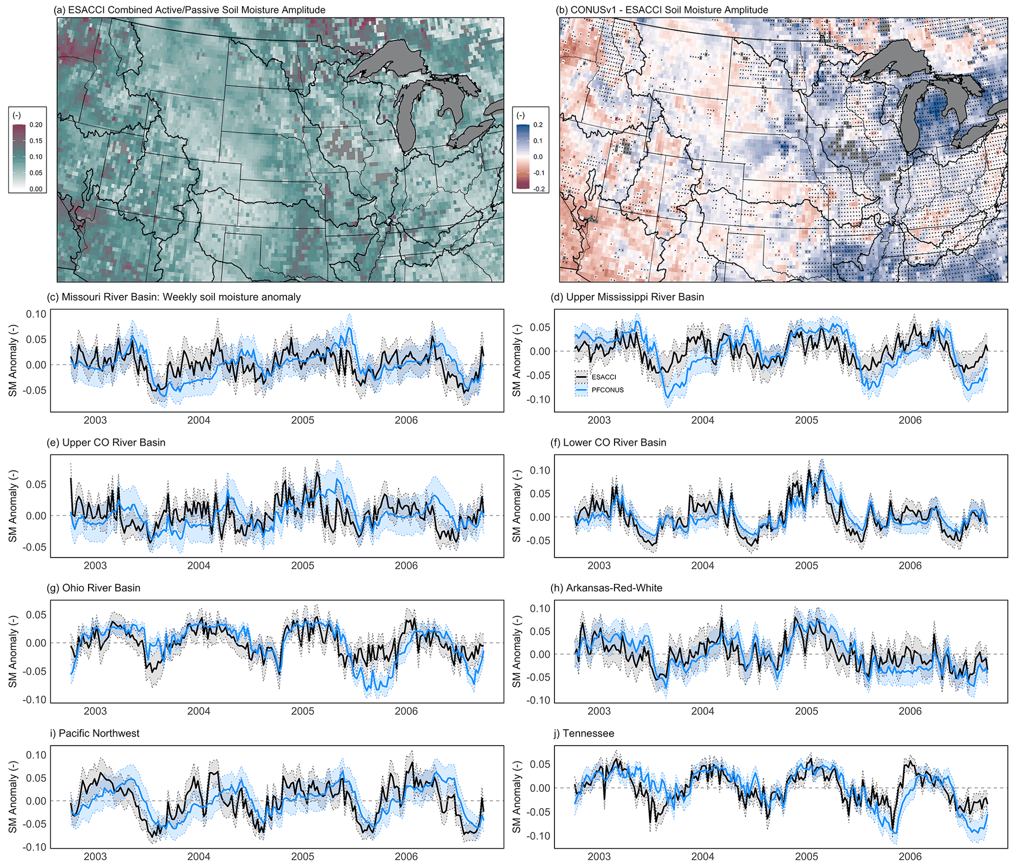
Figure 9Summary of ESACCI and PFCONUSv1 soil moisture comparisons. Seasonal SM amplitude for (a) the ESACCI solution and (b) PFCONUSv1–ESACCI amplitude difference. Stippling in (b) indicates that the ESACCI product time series was less than 50 % complete during the simulation period (fewer than 750 available observation days). Grey areas (excluded) indicate that the average ESACCI annual cycle had at least 3 months with zero available observations (and therefore the annual amplitude is uncertain). (c–h) Time series of weekly SM anomalies across complete major basins in the CONUSv1 domain. Shaded regions indicate ± 1 standard deviation taken spatially across the basin.
3.4.2 Soil moisture, Ssoil
Soil moisture (SM) anomalies (analogous to Ssoil) at the top layer of PFCONUSv1 (up to 0.1 m depth) were compared to the ESA CCI soil moisture product at 0.25∘ resolution and aggregated to weekly totals. Results are shown in Fig. 9. As in GRACE comparisons, we compared seasonal amplitude spatial signals across the PFCONUSv1 domain and basin-scale aggregates through time. The ESA CCI record is a state-of-the-art, multi-decadal, global satellite observation of SM created from combining single-sensor active and passive microwave sensors; since its release, the literature has shown good agreement between the ESA CCI product and spatial and LSM-modeled temporal SM patterns of soil moisture, and the harmonized product has shown better performance than any of its individual single-sensor inputs (Dorigo et al., 2017; Gruber et al., 2019). Because we are interested in ΔSsoil over time rather than the total water stored in the soil at any one moment, comparisons were made to SM anomalies, or relative change in soil moisture with respect to the mean value.
Broadly speaking, the PFCONUSv1 shows overall lower amplitude in the west and higher amplitude in the east relative to the CCI product (Fig. 9a and b). While this could be a result of PFCONUSv1 bias in evapotranspiration or other fluxes in which seasonal signal is dominant, it is also possible that amplitude differences are simply a result of temporal coverage or blending algorithms in the ESA CCI product. For instance, for the combined SM product, blending weights are higher for active microwave sensors in the eastern US and high-elevation Rockies, while the rest of the southwest and the northern Great Plains region favored passive microwave sensors (Dorigo et al., 2017). Further, ESA CCI SM is limited by temporal coverage; note that in the majority of the eastern PFCONUSv1 domain, fewer than 365 observation days are available (most likely a product of high humidity and cloud cover) (Fig. 9b), which makes us less confident in Ssoil amplitude estimates.
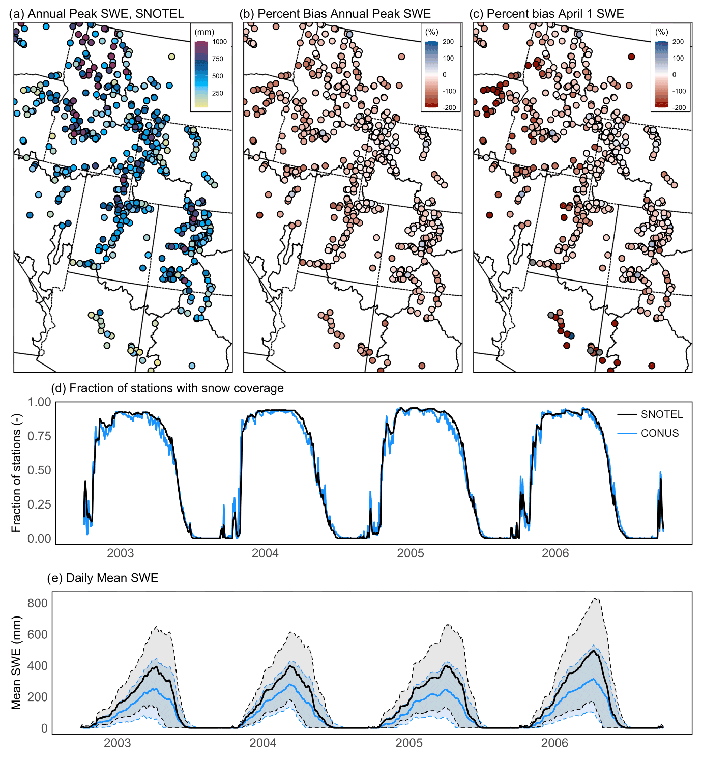
Figure 10Summary of PFCONUSv1-modeled snow water equivalent performance relative to SNOTEL sites. Shown are observed peak SWE at SNOTEL sites (a), percent bias for peak SWE (b) and 1 April SWE (c), daily spatial fraction of stations with snow coverage (d), and mean daily SWE (e). In (e), shaded regions indicate ± 1 standard deviation in space.
At the aggregated basin scale, however, temporal progression of SM shows temporal agreement between PFCONUSv1 and CCI SM for most major basins: individual ρ values for major basins are 0.25 (Upper Colorado), 0.79 (Lower Colorado), 0.75 (Arkansas–Red–White), 0.75 (Ohio), 0.43 (Missouri), 0.65 (Great Basin), 0.72 (Tennessee), and 0.55 (Upper Mississippi). The very weak correlation in the Upper Colorado basin may be indicative of large uncertainties in the ESA CCI SM product that have been observed with particular surface conditions: for regions of dense vegetation, topographic complexity, snow cover, or frozen soils, uncertainty in ESA CCI SM is very high (Dorigo et al., 2017), and we therefore have low confidence in ESACCI comparisons in Rocky Mountain headwater regions.
3.4.3 Snow water equivalent, Ssnow
Finally, the modeled PFCONUSv1 Ssnow storage component was validated against snow telemetry data in the mountainous west of the model domain (Fig. 10). An important caveat to note is that point-measured snow water equivalent (SWE) is likely to consistently overestimate gridded land surface model products, given that coarse-resolution model cells (in our case, 1 km lateral discretization) represent an aggregate of highly heterogenous SWE and canopy interference across a wide spatial area. Telemetry stations are frequently situated in clearings or in breaks in canopy density in order to maximize throughfall. For instance, Molotch and Bales (2005) characterized the distribution of SWE depth in 16, 4, and 1 km2 grid elements surrounding SNOTEL stations in Rio Grande headwaters using a combination of field observations, remote sensing products, and snowpack mass balance modeling. They found that at the majority of the sites, the SNOTEL station represented high percentiles of SWE relative to the surrounding land area and that SNOTEL site conditions (such as vegetation density, solar radiation index, and terrain indices) were not representative of the vast majority of grid element space. In some regions, SNOTEL SWE was more than 200 % greater than the mean grid element value.
As would therefore be expected, the 1 km resolution PFCONUSv1 model underestimates annual peak SWE (snow water equivalent at maximum accumulation) and 1 April SWE (snow water equivalent during ablation). PBIAS for annual peak SWE was −50.6 %, −33.5 %, and −14.7 % at the 25th, 50th, and 75th percentiles, respectively. 1 April SWE PBIAS was similar, with some individual SNOTEL stations showing more than double the SWE compared to PFCONUSv1 simulations (Fig. 10c). However, the PFCONUSv1 model clearly captures timing for snow accumulation and ablation, with the fraction of snow-covered sites tracking almost identically between SNOTEL and PFCONUSv1 (Fig. 10d). Percentiles for Spearman's ρ values for cool season daily SWE (Fig. 10d) are 0.85 (25th percentile), 0.92 (50th), and 0.96 (75th).
In Sect. 3, outputs from an integrated surface water–groundwater hydrologic model, PFCONUSv1, were compared to available point-scale monitoring networks and remote sensing products in an effort to evaluate the model's ability to reliably reproduce components of the water budget listed in Eq. (1).
Table 2Examples of potential sources of bias acting on PFCONUSv1 results.
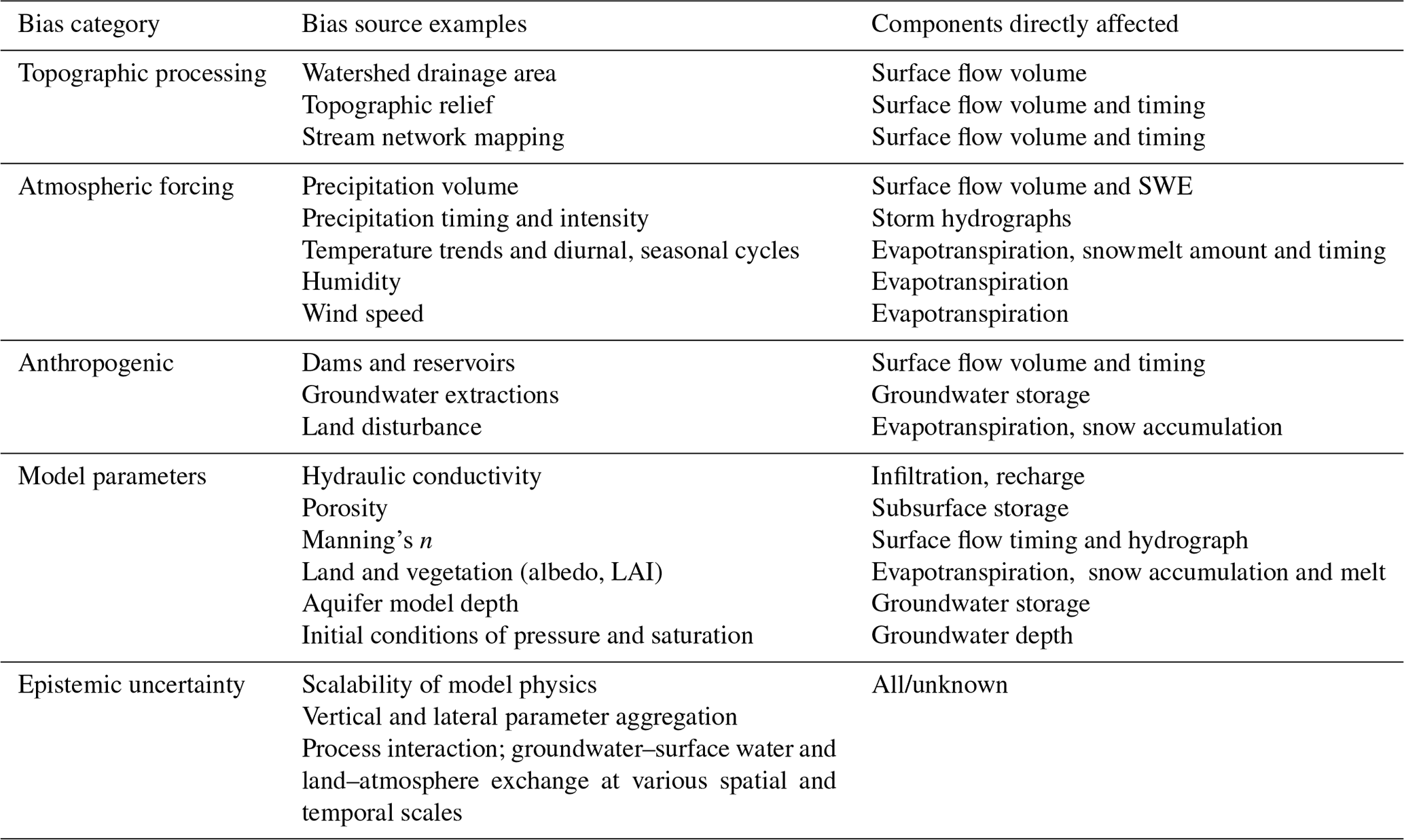
Broadly, results suggest that PFCONUSv1 shows promising ability to reproduce the timing, mean states, and inter- and intra-annual variability of continental-scale water balance components. However, the PFCONUSv1 model should be considered a work in progress; with approximately 31 million cells in the domain, PFCONUSv1 bias can originate from errors associated with model physics, inputs, process representation, or epistemic uncertainty (Table 2). The best publicly available datasets were used to populate and drive this simulation, but such inputs are certainly subject to their own errors and uncertainties and must be continuously revisited to improve their fidelity. In this section, we discuss identifiable errors in model inputs and implications for future model development.
4.1 Meteorological forcing errors and topographic processing
Major biases exist in preprocessing of PFCONUSv1 meteorological forcing and topography, which are peripheral to but act simultaneously with all other sources of bias (Table 2). In this way, isolating the effects of a single bias source can be challenging. Streamflow itself is sensitive to errors in drainage area, topographic relief, and precipitation or temperature bias, and the errors in surface and subsurface moisture flux can propagate downstream to impact moisture availability and evapotranspiration in areas remote from the original bias source.
4.1.1 Terrain processing and drainage area
Topographic slopes were defined from a digital elevation model (DEM) generated by HydroSHEDS and subsequently subjected to a hydrologic processing algorithm, which adjusted drainage networks to remove true and artificial pits, depressions, and barriers and ensure complete river network connectivity (Barnes et al., 2016). However, both loss of resolution in DEMs and the topographic processing can result in loss of topographic relief and change in drainage area. Therefore, PFCONUSv1 streamflow percent bias should in theory reflect fidelity of upstream watershed area. We compared PFCONUSv1 drainage area with “true” drainage area determined based on geospatial stream properties obtained from the GAGES-II (Falcone, 2002).
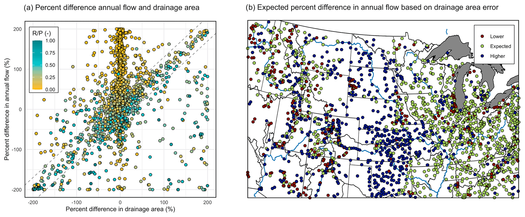
Figure 11(a) Percent difference between observed and simulated annual flow volume as a function of percent difference in true and PFCONUSv1 drainage area, colored by annual runoff ratio. (b) Locations where error in simulated flow volume is greater than, less than, or expected from drainage area bias. Expected behavior was defined as locations that lie within the ± 30 % dashed error bars shown in (a).
Figure 11 shows the relationship between percent difference in observed and simulated streamflow versus percent difference in observed and processed drainage area for all 2392 USGS stream gauges. There are three primary conclusions to be drawn from this relationship (Fig. 11a): (1) a clear, linearly proportional correlation exists between percent difference in drainage and percent difference in streamflow. For streamflow percent difference from observed ranging from −200 % to 200 %, we find that 977 out of 2392 stream gauges fall within ± 30 % of this flow–drainage relationship. Essentially, this means that for 41 % of gauges in PFCONUSv1, the percent bias in annual flow can be primarily attributed to errors in topographic processing. (2) A considerable number of gauges exhibit positive percent difference between observed and simulated annual streamflow, and these gauges are typically those with very low runoff ratios. Such a finding is not surprising in that streams with low RR will be particularly sensitive to external drivers. And (3) a certain amount of noise exists in these drainage–flow relationships, with many locations exhibiting higher or lower error in annual flow than that expected by drainage errors regardless of runoff ratio.
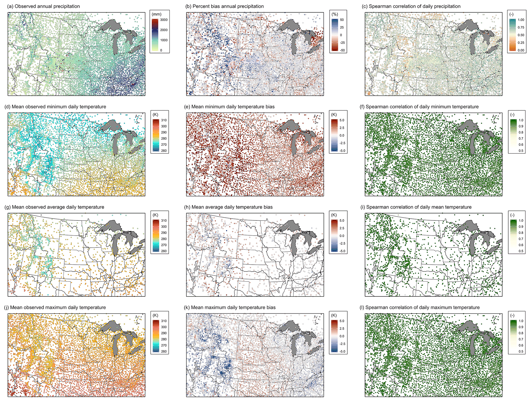
Figure 12Observed precipitation and temperature at GHCND meteorological stations compared to interpolated NLDAS at their nearest-neighbor PFCONUSv1 cell. (a) Observed cumulative annual precipitation, (b) percent bias in annual precipitation, (c) Spearman's ρ between simulated and observed daily precipitation. Also shown are observed average daily minimum (d), average (g), and maximum (j) temperature, the total bias in minimum (e), average (h), and maximum daily temperature (k), and the Spearman correlation for minimum (f), average (i), and maximum (l) daily temperature.
Figure 11b shows locations where the flow–drainage relationship was expected or unexpected. For the majority of the eastern United States, bias in streamflow is simply a function of drainage area bias from topographic processing. The mountainous west was considerably noisier, exhibiting in somewhat equal parts lower, higher, or expected annual flow behavior from drainage bias. We expect that much of the noise in annual flow bias is a function of precipitation and temperature bias and timing and, subsequently, snowpack. However, in the Great Plains region, the considerable positive annual flow bias shown in Fig. 3 cannot be attributed to the error in drainage area. In fact, for 600 gauges in the Great Plains area (∼ 20 % of all locations), the percent difference between PFCONUSv1 and true drainage area is near 0, but percent difference in streamflow is between 30 and 200 %. We believe that the greatest driver of this bias is the lack of groundwater extractions in the PFCONUSv1 model. Note that not only is the PFCONUSv1 model naturalized for the 2002–2006 simulation period, but its initial condition is also informed by 1985 naturalized spin-up, which does not include at least 50 years of groundwater depletion. However, some of the positive annual flow bias behavior in this region could be attributed to some biases in cumulative precipitation, which is detailed in Sect. 4.1.2.
4.1.2 Atmospheric forcing bias
The NLDAS meteorological forcing, which is described in Sect. 2.2, was bilinearly interpolated across the PFCONUSv1 domain; biases in precipitation, evaporation, wind speed, humidity, and radiation can therefore come from either the NLDAS product or its statistical downscaling. We compared daily total precipitation and average daily air temperature from the interpolated NLDAS product at 9139 (P) and 1678 (temperature) GHCND meteorological stations across the PFCONUSv1 domain by calculating relative bias and Spearman's ρ at each location. Figure 12 summarizes these comparisons. Broadly, we can identify several examples for which NLDAS biases are potential drivers of the bias in timing and volume of hydrologic fluxes.
PFCONUSv1 annual precipitation over the Kansas–Nebraska border in the Great Plains region is 10 %–25 % greater than observed (Fig. 12b). This bias could be one source of positive flow bias at USGS stream gauges east of the High Plains aquifer.
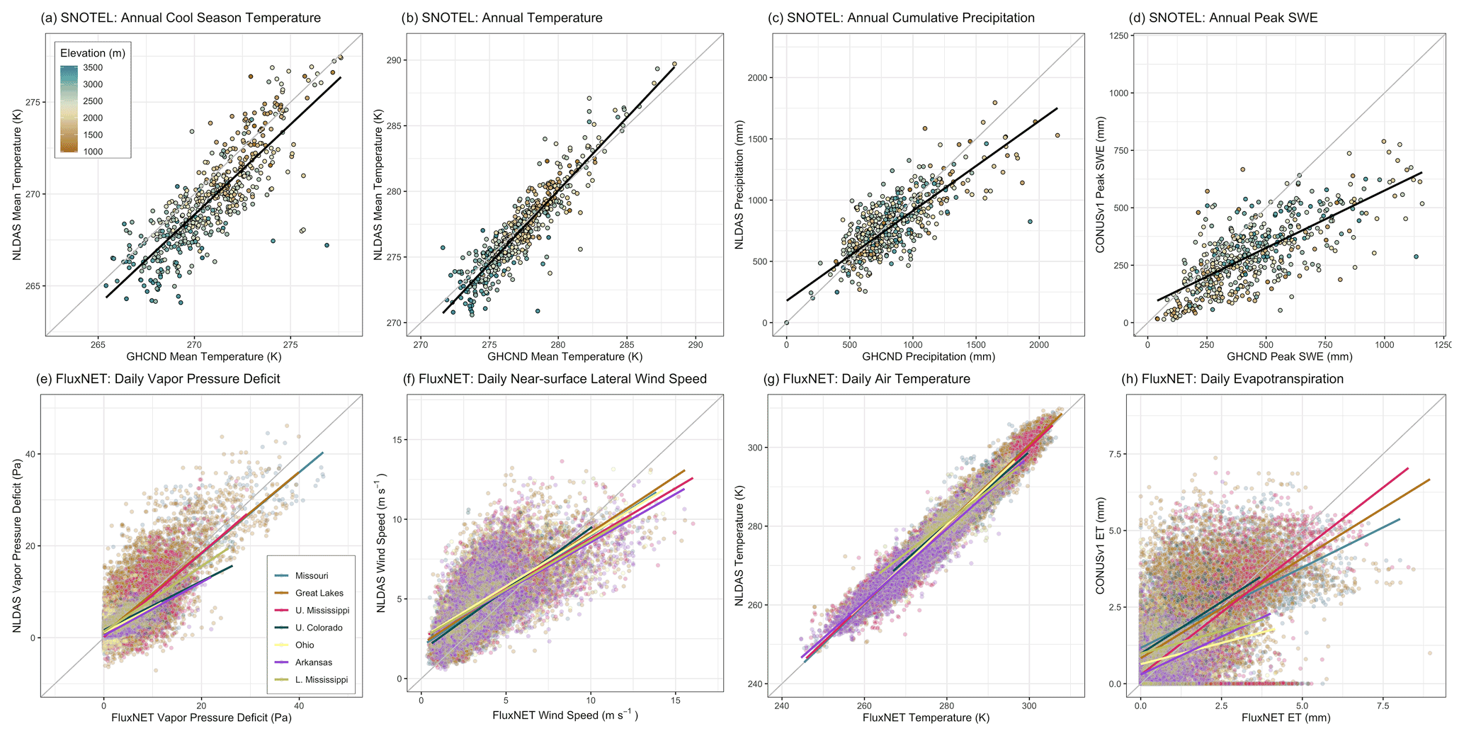
Figure 13Meteorological forcing, SWE, and ET bias at SNOTEL and FLUXNET stations. At SNOTEL locations, colored by elevation: (a) mean NLDAS mean cool season temperature versus observed cool season temperature, (b) mean NLDAS annual temperature versus observed cool season temperature, (c) NLDAS annual cumulative precipitation versus observed, and (d) PFCONUSv1 annual peak SWE versus observed. At FLUXNET locations, colored by the major basin location of the FLUXNET site: (e) daily NLDAS vapor pressure deficit versus observed, (f) daily NLDAS near-surface lateral wind speed versus observed, (g) daily NLDAS mean air temperature versus observed, and (h) PFCONUSv1 daily ET versus observed. Lines show linear regression with p<0.05 in all cases.
Fidelity in streamflow timing will of course be a function of accurate precipitation timing and intensity. A hydrologic model cannot be expected to perform considerably better than its recharge forcing, or results could be considered spurious. Areas with the weakest correlation between observed and NLDAS daily precipitation are in the Rocky Mountain headwater region (Fig. 12c). In the Upper Colorado watershed as a whole, the 50th percentile ρ value for daily precipitation is 0.56, or the lowest of all other major basins. The Upper Colorado is also the basin with poorest overall daily streamflow timing, with ρ50th = 0.33.
Our interpolated NLDAS product underestimates the diurnal temperature fluctuations, primarily by considerably overestimating minimum (nighttime) daily temperature (Fig. 12e), which is likely a considerable driver of underestimated SWE. Further, maximum daily temperature is underestimated over the Rockies (Fig. 12h). Given that ET is largely dependent upon available radiative forcing, this could explain some of PFCONUSv1 negative bias at FLUXNET stations over the Rockies.
Annual temperature errors could also explain several regions where PFCONUSv1 comparisons to MOD16A2 and to SSEBop MODIS algorithms agree. For example, warm temperature biases and positive ET biases (relative to both MODIS algorithms; Fig. 6g and h) are seen in much of the lower elevations of the mountainous west and in the majority of the Pacific Northwest. Spatial patterns of ET biases (Fig. 7g and h) in the Upper Mississippi and Ohio River basins seem to instead follow the spatial pattern of precipitation bias (Fig. 11b), with regions receiving higher precipitation also experiencing higher ET.
NLDAS-simulated daily temperature timing is excellent. However, temperature was not deseasonalized before correlation was calculated, and the seasonal signal will certainly account for the majority of temperature variance.
More specifically, we can verify specific impacts of NLDAS bias on SWE and ET at individual SNOTEL and FLUXNET sites. Figure 13 shows observed and simulated (or interpolated) meteorological conditions and water balance components for snow and evapotranspiration.
SWE bias at SNOTEL sites is preferentially low at higher elevations (Fig. 13d). While this difference, as discussed above, can to a certain extent be attributed to differences in heterogeneous land and vegetation between the point and grid scale (Molotch and Bales, 2005), we also find that biases in temperature and precipitation likely drive the PFCONUSv1 low bias in snowpack. PFCONUSv1 SWE experiences a low bias in cumulative annual precipitation at SNOTEL sites (Fig. 13c), and lower elevations exhibit a warm cool season and annual temperature bias (Fig. 13a and b), both of which would contribute to low accumulation and high ablation rates.
While NLDAS shows good agreement with observed FLUXNET temperature (Fig. 13g), comparisons between NLDAS and observed vapor pressure deficit and wind speed both exhibit a considerable amount of scatter (Fig. 13e and f). Overall, the poorest-performing sites for vapor pressure (those in the Upper Colorado River basin) also exhibited the highest-magnitude ET biases (Fig. 13h). PFCONUSv1 underestimates (overestimates) relatively high (low) daily evapotranspiration rates (Fig. 13h). For FLUXNET locations and days exhibiting ET rates over (under) 4 mm d−1, mean daily bias is −1.2 mm (0.3 mm). Biases in NLDAS vapor pressure and wind speed could be a contributing factor. Lower vapor pressure deficits (0 to 20 Pa) and lower wind speeds (0 to 6 m s−1) have an overall positive bias and could explain PFCONUSv1 overpredicting low ET days. Similarly, we believe the bias on high-evapotranspiration days (ET > 4 mm d−1), which PFCONUSv1 preferentially underpredicts, could be attributed to NLDAS underpredicting wind speeds greater than ∼ 10 m s−1.
Errors in atmospheric forcing products often necessitate statistical bias correction before simulations are run (Piani et al., 2010). NLDAS has been specifically validated in its ability to reproduce meteorological conditions for streamflow (Xia et al., 2012a), soil moisture (Xia et al., 2015a), and evapotranspiration (Xia et al., 2015b) prediction by LSMs. While long-term spatial patterns and seasonal signals were captured for soil moisture and evapotranspiration, NLDAS fidelity at daily or weekly timescales is less certain. In this study, it is difficult to directly attribute the portion of streamflow, SWE, or ET errors that occur from atmospheric forcing bias, but these water balance components would certainly improve with continued progress in meteorological forcing datasets. The ParFlow–CLM water budget has been shown to be particularly sensitive to uncertainty in both precipitation and temperature forcings in mountainous regions, largely due to their additive influence on snow accumulation, melt, and subsequent mountain block recharge (Schreiner-McGraw and Ajami, 2021). Other studies have also highlighted the persistent biases in precipitation and temperature estimates from continental or global meteorological products, which can propagate into hydrologic model predictions (e.g., Ashfaq et al., 2010; Sperna Weiland et al., 2015).
4.2 Anthropogenic process representation and other epistemic errors
Plenty of sources of uncertainty can contribute to biases not discussed in Sect. 4.1 (Table 2). We have chosen to address meteorological forcing and topographic processing errors above simply because they are somewhat readily quantifiable, while parameter values and other epistemic uncertainties, such as simplification or scaling of model physics, are poorly constrained or simply unknown. Other biases include population of model parameter fields.
While we do not discuss model parameter uncertainty, such as conductivity, porosity, van Genuchten parameters, Manning's surface roughness, land and vegetation parameters, or model horizontal and vertical discretization, these are also areas for improvement. For example, Maxwell et al. (2015) show that national geologic and soil parameter datasets are prone to errors via political boundaries, such as state lines, and the PFCONUSv1 model oversimplifies deeper geology, with a 100 m vertically homogenous layer.
However, as mentioned above, these fields are poorly constrained at the continental scale, and simulations are necessarily limited by availability of appropriate distributed products. Model parameter population is often addressed through calibration, but population of parameter fields becomes increasingly difficult as resolution increases and calibration becomes more computationally demanding. Future model iterations may need to take advantage of methods that allow transfer of parameters (e.g., conductivity) from coarse-resolution, efficient models to high-resolution ones (Foster and Maxwell, 2019). Model discretization is another concern. Coarsening of vertical and lateral resolution is a necessity at the continental scale, but aggregating to ∼ 1 km resolution certainly comes with inherent uncertainties and loss of information. DEMs in particular will lose topographic drivers with scale (Wu et al., 2008), resulting in loss of relief; on the other hand, coarse-resolution cells could result in inappropriately steep pressure gradients as a function of Richards' equation parameterization and pressure-dependent permeability (Maxwell and Condon, 2016), and suitable vertical length scales for Richards' equations generally do not exceed several meters (Or et al., 2015). This calls into question the scalability of model physics; as Beven and Cloke (2012) rightly point out, whether or not governing partial differential equations will scale linearly is a concern. However, the current governing equations for PFCONUSv1 are simply the best currently known representation of hydrologic processes at this scale.
Finally, process representation is certainly a concern. Transient anthropogenic modules, such as urban hydrology models, pumping and injections, or surface water diversions, are currently possible but add to computational demand and require detailed historical data on water use with temporal and spatial coverage simply not yet available. As a naturalized model, the PFCONUSv1 simulations presented here will necessarily overpredict water tables and baseflow in regions where extractions are apparent. For instance, Maxwell and Condon (2016, supplemental information) show streamflow examples at the Lees Ferry USGS gauge, where timing and volume of streamflow are entirely governed by dam hydraulics. Condon and Maxwell (2019) show that incorporating a century of groundwater depletion across the PFCONUSv1 domain considerably decreases streamflow, with sensitivity to pumping concentrating downstream; more specifically, they found that long-term depletions over the High Plains aquifer resulted in a swap of discharging to recharging groundwater. However, naturalized continental models with high fidelity in non-anthropogenic settings could be used to estimate impact from human influence simply by examining the difference between observed and simulated conditions.
In this study, we present the detailed evaluation of a transient, coupled hydrologic–land surface simulation at the continental scale and at hyper-resolution using a diverse set of monitoring networks and state-of-the-art remote sensing products. We found that PFCONUSv1 reproduced temporal patterns for continental-scale water budget components with an accuracy of at least ρ = 0.5. The following are 50th percentile (in space, over the entire domain) Spearman's rank correlations ρ for individual water balance components: ρ50th = 0.65 for R, with evaluation against daily USGS stream gauge observations; ρ50th = 0.72 for ET, with evaluation against daily FLUXNET eddy covariance observations (for monthly HUC8-aggregated remote sensing products, ρ50th = 0.85 for ET relative to MOD16A2 algorithm, and ρ50th = 0.91 for ET relative to SSEBop algorithm); ρ50th = 0.80 for major basin-aggregate S, with evaluation against monthly GRACE remote gravity field sensing; ρ50th = 0.46 for filtered USGS well observations, which are related but not equivalent to Sgw; ρ50th = 0.69 for major basin-aggregate Ssoil, with evaluation against ESA CCI weekly SM from active/passive microwave sensors (Upper Colorado is not excluded, but note the uncertainties in ESA CCI over snow-covered, densely forested, and topographically complex land area); and ρ50th = 0.92 for Ssnow, with evaluation against daily SNOTEL point observations. In terms of temporally aggregated annual fluxes, which represent long-term water budget component states, PFCONUSv1 simulates 50th percentile |PBIAS| of 41.3 % for streamflow relative to USGS gauges: 14.2 % for ET relative to MOD16A2 and 13.2 % for ET relative to SSEBop at the aggregated monthly and HUC8 scales, 37.9 % for ET relative to FLUXNET sites, and 35.3 % for peak annual SWE relative to SNOTEL locations. We also found RSR for PFCONUSv1 performance at point locations, with RSR50th = 0.92 at FLUXNET sites and RSR50th = 1.2 at USGS streams, while RSR values for PFCONUSv1 relative to MODIS products aggregated at the monthly and HUC8 scale are 0.85 and 0.47 for MOD16A2 and SSEBop, respectively. Performance varies widely across the model domain, with the eastern United States showing better overall performance at USGS stream gauges and relative to MODIS remote sensing products than the western US. In terms of S, PFCONUSv1-simulated SM is best for the Tennessee, Ohio, and Lower Colorado River basins relative to the spatially aggregated ESACCI soil moisture product; total water storage performance is best for the Upper Mississippi River basin relative to the GRACE TWS anomaly products. Further, we discussed three primary sources of model bias: terrain processing, errors in atmospheric forcing, and lack of anthropogenic influence.
The results presented here provide benefits to the high-resolution, continental-scale (and above) hydrologic community. First, our level of agreement with observations and remote sensing products suggests great promise for extreme-scale and high-resolution modeling to become a reality. We argue that PFCONUSv1 and similar models are feasible and will certainly see improvements in the near future with increased availability of open-access and distributed datasets, remote sensing advancements, improved monitoring networks, and advancements in highly parallelized computing.
Second, these results provide a guide for PFCONUS development. Some areas for model improvement that were immediately identified in this study include the following: (1) the source of high positive bias in the Central Plains should be further addressed. While we propose that this bias is largely attributed to the lack of groundwater pumping in the model (we estimate that at least 25 % of stream gauges are impacted by High Plains aquifer depletions), other potential sources of error could include inappropriate soil or geology hydraulic conductivity or van Genuchten parameters, the lack of spatially distributed Manning's coefficient (Maxwell et al., 2015), or loss of topographic relief associated with 1 km lateral resolution. (2) We show that topographic processing has resulted in considerable error in drainage area for approximately 40 % of stream gauges. Accessible improvements could be made to streamflow bias with improved topographic processing algorithms. And (3) interpolated atmospheric forcing from NLDAS reanalysis has two primary biases that, if corrected with statistical bias correction or other methods, would immediately benefit streamflow, ET, and snow water equivalent. First, precipitation timing is lacking in many areas of the domain, particularly over the Rocky Mountain region. Second, mean nighttime air temperature exhibits a high temperature bias, resulting in an underestimated diurnal temperature fluctuation for the majority of the domain. Average daytime maximum temperature is also underestimated over the Rocky Mountains.
Finally, we argue that model fidelity can only be reliably understood at a process-based level if all water balance components available in the model outputs are evaluated. While single-parameter validation may be effective for operational forecasts, we do risk the equifinality dilemma of arriving at the right answer for the wrong reasons (Kirchner, 2006). The value in the type of validation exercise presented here is clearly a mechanistic understanding of model performance and a higher level of confidence in overall water balance modeling skill. Further work should be done to continue to incorporate additional observational and remote sensing networks as they become available. Also, while explicit comparisons with observations and simulations, like those presented here, are valuable, comparisons with other models are equally an asset used to build confidence in the plausibility of parameterization, outputs, and their mechanistic relationships. Gleeson et al. (2021) stress the importance of model intercomparison projects, such as IH-MIP2 (Kollet et al., 2017), as tools for model evaluation for global groundwater simulations. Impressive model validation toolkits that exist in the land surface community, such as the Land surface Validation Toolkit (LVT) (Kumar et al., 2012) and the International Land Model Benchmarking (ILAMB) system (Collier et al., 2018), as well as nascent model comparisons in the continental hydrology community, such as the Continental Hydrologic Intercomparison Project (CHIP) (Tijerina et al., 2021), are inspiring collaborative efforts to streamline and standardize model evaluation. We hope to take advantage of the LVT and ILAMB platforms in the future to compare model performance to other similar continental- and global-scale simulations, to standardize our model evaluation, and to add to our existing observation datasets. Further work is also needed to assess the scale gaps prevalent in observation and remote sensing data. Specifically, point-scale observations sensitive to small-scale heterogeneity, such as in situ soil moisture observations, are unlikely to be applicable to the 1 km scale, resulting in commensurability errors (Gleeson et al., 2021); conversely, we cannot guarantee that PFCONUSv1 outputs scale linearly to coarser-resolution products and models. Improved understanding of how model bias scales with loss of spatial or temporal resolution is a vital area of research.
ParFlow–CLM is an open-source, parallel, modular hydrologic model that is freely available on GitHub at https://github.com/parflow/parflow.git (last access: 4 March 2021). The version of ParFlow–CLM used in this study, v3.6, is archived on Zenodo at https://doi.org/10.5281/zenodo.4639761 (Smith et al., 2019). All data generated from the ParFlow–CLM CONUS configuration version 1.0 are available upon request. Given the considerable storage demand (approximately 60 TB for 4 water years of hourly data, including forcing and daily or monthly processed climatologies), the model outputs are stored on a private server. The authors will coordinate with the HydroFrame project team, funded through the NSF Cyberinfrastructure for Sustained Scientific Innovation (CSSI) project, to ultimately provide a FAIR-aligned, publicly accessible data repository of all raw model results. A primary objective of the HydroFrame project is to provide a platform for users to freely access PFCONUS model results, as well as to subset or modify inputs and forcing to locally run their own ParFlow–CLM simulations. As HydroFrame capabilities develop and future versions are completed, we plan to make PFCONUS results publicly available through this platform.
The supplement related to this article is available online at: https://doi.org/10.5194/gmd-14-7223-2021-supplement.
MMFO'N prepared and ran PFCONUSv1 simulations, processed model outputs, analyzed model performance, and prepared the paper with contributions from coauthors. RMM and LEC provided some processing codes for spatiotemporal averaging, offered guidance for interpreting integrated hydrologic simulations and managing data, and aided in paper preparation and editing. DTT contributed to paper preparation, editing, and review.
The authors declare that they have no conflict of interest.
Publisher's note: Copernicus Publications remains neutral with regard to jurisdictional claims in published maps and institutional affiliations.
The authors gratefully acknowledge the high-performance computing resources provided by the National Center for Atmospheric Research (NCAR) Computational and Information Systems Laboratory (CISL) Cheyenne computing platform. The authors also thank the editor and two anonymous referees for their expertise and constructive feedback during the review process.
This research has been supported by the National Science Foundation Office of Advanced Cyberinfrastructure, Cyberinfrastructure for Sustained Scientific Innovation (CSSI) project (grant no. 1835903) and the US Department of Energy Interoperable Design of Extreme-scale Application Software (IDEAS) project (grant no. DE-AC02-05CH11231).
This paper was edited by Richard Mills and reviewed by two anonymous referees.
Archfield, S. A., Clark, M., Arheimer, B., Hay, L. E., McMillan, H., Kiang, J. E., Seibert, J., Hakala, K., Bock, A., Wagener, T., Farmer, W. H., Andréassian, V., Attinger, S., Viglione, A., Knight, R., Markstrom, S., and Over, T.: Accelerating advances in continental domain hydrologic modeling, Water Resour. Res., 51, 10078–10091, https://doi.org/10.1002/2015WR017498, 2015.
Ashfaq, M., Bowling, L. C., Cherkauer, K., Pal, J. S., and Diffenbaugh, N. S.: Influence of climate model biases and daily-scale temperature and precipitation events on hydrological impacts assessment: A case study of the United States, J. Geophys. Res., 115, D14116, https://doi.org/10.1029/2009JD012965, 2010.
Bai, P., Liu, X., Yang, T., Liang, K., and Liu, C.: Evaluation of streamflow simulation results of land surface models in GLDAS on the Tibetan plateau, J. Geophys. Res.-Atmos., 121, 12180–12197, https://doi.org/10.1002/2016JD025501, 2016.
Baldocchi, D. D.: Assessing the eddy covariance technique for evaluating carbon dioxide exchange rates of ecosystems: past, present and future, Glob. Change Biol., 9, 479–492, https://doi.org/10.1046/j.1365-2486.2003.00629.x, 2003.
Barnes, M. L., Welty, C., and Miller, A. J.: Global Topographic Slope Enforcement to Ensure Connectivity and Drainage in an Urban Terrain, J. Hydrol. Eng., 21, 06015017, https://doi.org/10.1061/(ASCE)HE.1943-5584.0001306, 2016.
Beck, H. E., van Dijk, A. I. J. M., de Roo, A., Miralles, D. G., McVicar, T. R., Schellekens, J., and Bruijnzeel, L. A.: Global-scale regionalization of hydrologic model parameters, Water Resour. Res., 52, 3599–3622, https://doi.org/10.1002/2015WR018247, 2016.
Beven, K. J. and Cloke, H. L.: Comment on “Hyperresolution global land surface modeling: Meeting a grand challenge for monitoring Earth's terrestrial water” by Eric F. Wood et al., Water Resour. Res., 48, W01801, https://doi.org/10.1029/2011wr010982, 2012.
Bierkens, M. F. P., Bell, V. A., Burek, P., Chaney, N., Condon, L. E., David, C. H., de Roo, A., Döll, P., Drost, N., Famiglietti, J. S., Flörke, M., Gochis, D. J., Houser, P., Hut, R., Keune, J., Kollet, S., Maxwell, R. M., Reager, J. T., Samaniego, L., Sudicky, E., Sutanudjaja, E. H., van de Giesen, N., Winsemius, H., and Wood, E. F.: Hyper-resolution global hydrological modelling: what is next?, Hydrol. Process., 29, 310–320, https://doi.org/10.1002/hyp.10391, 2015.
Chen, J., Famigliett, J. S., Scanlon, B. R., and Rodell, M.: Groundwater Storage Changes: Present Status from GRACE Observations, Springer, Cham, https://doi.org/10.1007/978-3-319-32449-4_9, pp. 207–227, 2016.
Clark, M. P., Fan, Y., Lawrence, D. M., Adam, J. C., Bolster, D., Gochis, D. J., Hooper, R. P., Kumar, M., Leung, L. R., Mackay, D. S., Maxwell, R. M., Shen, C., Swenson, S. C., and Zeng, X.: Improving the representation of hydrologic processes in Earth System Models, Water Resour. Res., 51, 5929–5956, https://doi.org/10.1002/2015WR017096, 2015.
Collier, N., Hoffman, F. M., Lawrence, D. M., Keppel-Aleks, G., Koven, C. D., Riley, W. J., Mu, M., and Randerson, J. T.: The International Land Model Benchmarking (ILAMB) System: Design, Theory, and Implementation, J. Adv. Model. Earth Sy., 10, 2731–2754, https://doi.org/10.1029/2018MS001354, 2018.
Condon, L. E. and Maxwell, R. M.: Evaluating the relationship between topography and groundwater using outputs from a continental-scale integrated hydrology model, Water Resour. Res., 51, 6602–6621, https://doi.org/10.1002/2014WR016774, 2015.
Condon, L. E. and Maxwell, R. M.: Systematic shifts in Budyko relationships caused by groundwater storage changes, Hydrol. Earth Syst. Sci., 21, 1117–1135, https://doi.org/10.5194/hess-21-1117-2017, 2017.
Condon, L. E. and Maxwell, R. M.: Simulating the sensitivity of evapotranspiration and streamflow to large-scale groundwater depletion, Science Advances, 5, eaav4574, https://doi.org/10.1126/sciadv.aav4574, 2019.
Condon, L. E., Hering, A. S., and Maxwell, R. M.: Quantitative assessment of groundwater controls across major US river basins using a multi-model regression algorithm, Adv. Water Resour., 82, 106–123, https://doi.org/10.1016/J.ADVWATRES.2015.04.008, 2015.
Condon, L. E., Atchley, A. L., and Maxwell, R. M.: Evapotranspiration depletes groundwater under warming over the contiguous United States, Nat. Commun., 11, 1–8, https://doi.org/10.1038/s41467-020-14688-0, 2020.
Cosgrove, B. A.: Real-time and retrospective forcing in the North American Land Data Assimilation System (NLDAS) project, J. Geophys. Res., 108, 8842, https://doi.org/10.1029/2002JD003118, 2003.
Dahle, C., Murböck, M., Flechtner, F., Dobslaw, H., Michalak, G., Neumayer, K., Abrykosov, O., Reinhold, A., König, R., Sulzbach, R., and Förste, C.: The GFZ GRACE RL06 Monthly Gravity Field Time Series: Processing Details and Quality Assessment, Remote Sens.-Basel, 11, 2116, https://doi.org/10.3390/rs11182116, 2019.
Dai, Y., Zeng, X., Dickinson, R. E., Baker, I., Bonan, G. B., Bosilovich, M. G., Denning, A. S., Dirmeyer, P. A., Houser, P. R., Niu, G., Oleson, K. W., Schlosser, C. A., and Yang, Z.-L.: The Common Land Model, B. Am. Meteorol. Soc., 84, 1013–1024, https://doi.org/10.1175/BAMS-84-8-1013, 2003.
de Graaf, I. E. M., van Beek, R. L. P. H., Gleeson, T., Moosdorf, N., Schmitz, O., Sutanudjaja, E. H., and Bierkens, M. F. P.: A global-scale two-layer transient groundwater model: Development and application to groundwater depletion, Adv. Water Resour., 102, 53–67, https://doi.org/10.1016/j.advwatres.2017.01.011, 2017.
Döll, P., Kaspar, F., and Lehner, B.: A global hydrological model for deriving water availability indicators: Model tuning and validation, J. Hydrol., 270, 105–134, https://doi.org/10.1016/S0022-1694(02)00283-4, 2003.
Döll, P., Fritsche, M., Eicker, A., and Müller Schmied, H.: Seasonal Water Storage Variations as Impacted by Water Abstractions: Comparing the Output of a Global Hydrological Model with GRACE and GPS Observations, Surv. Geophys., 35, 1311–1331, https://doi.org/10.1007/s10712-014-9282-2, 2014.
Dorigo, W., Wagner, W., Albergel, C., Albrecht, F., Balsamo, G., Brocca, L., Chung, D., Ertl, M., Forkel, M., Gruber, A., Haas, E., Hamer, P. D., Hirschi, M., Ikonen, J., de Jeu, R., Kidd, R., Lahoz, W., Liu, Y. Y., Miralles, D., Mistelbauer, T., Nicolai-Shaw, N., Parinussa, R., Pratola, C., Reimer, C., van der Schalie, R., Seneviratne, S. I., Smolander, T., and Lecomte, P.: ESA CCI Soil Moisture for improved Earth system understanding: State-of-the art and future directions, Remote Sens. Environ., 203, 185–215, https://doi.org/10.1016/j.rse.2017.07.001, 2017.
Falcone, J. A.: GAGES-II: Geospatial attributes of gages for evaluating streamflow, U.S. Geological Survey, available at: https://water.usgs.gov/GIS/metadata/usgswrd/XML/gagesII_Sept2011.xml (last access: 18 August 2020), 2002.
Fan, Y., Li, H., and Miguez-Macho, G.: Global patterns of groundwater table depth, Science, 339, 940–943, https://doi.org/10.1126/science.1229881, 2013.
Finger, D., Vis, M., Huss, M., and Seibert, J.: The value of multiple data set calibration versus model complexity for improving the performance of hydrological models in mountain catchments, Water Resour. Res., 51, 1939–1958, https://doi.org/10.1002/2014WR015712, 2015.
Foster, L. M. and Maxwell, R. M.: Sensitivity analysis of hydraulic conductivity and Manning's n parameters lead to new method to scale effective hydraulic conductivity across model resolutions, Hydrol. Process., 33, https://doi.org/10.1002/hyp.13327, 332–349, 2019.
Gleeson, T., Smith, L., Moosdorf, N., Hartmann, J., Dürr, H. H., Manning, A. H., van Beek, L. P. H., and Jellinek, A. M.: Mapping permeability over the surface of the Earth, Geophys. Res. Lett., 38, L02401, https://doi.org/10.1029/2010GL045565, 2011.
Gleeson, T., Moosdorf, N., Hartmann, J., and van Beek, L. P. H.: A glimpse beneath Earth's surface: GLobal HYdrogeology MaPS (GLHYMPS) of permeability and porosity, Geophys. Res. Lett., 41, 3891–3898, https://doi.org/10.1002/2014GL059856, 2014.
Gleeson, T., Wagener, T., Döll, P., Zipper, S. C., West, C., Wada, Y., Taylor, R., Scanlon, B., Rosolem, R., Rahman, S., Oshinlaja, N., Maxwell, R., Lo, M.-H., Kim, H., Hill, M., Hartmann, A., Fogg, G., Famiglietti, J. S., Ducharne, A., de Graaf, I., Cuthbert, M., Condon, L., Bresciani, E., and Bierkens, M. F. P.: GMD Perspective: the quest to improve the evaluation of groundwater representation in continental to global scale models, Geosci. Model Dev. Discuss. [preprint], https://doi.org/10.5194/gmd-2021-97, in review, 2021.
Group on Earth Observations: GEOSS Strategic Targets, Document 12 (Rev1), GEO-VI, 17–18 November 2009, available at: https://www.earthobservations.org/documents.php (last access: 18 October 2021), 2009.
Gruber, A., Scanlon, T., van der Schalie, R., Wagner, W., and Dorigo, W.: Evolution of the ESA CCI Soil Moisture climate data records and their underlying merging methodology, Earth Syst. Sci. Data, 11, 717–739, https://doi.org/10.5194/essd-11-717-2019, 2019.
Gupta, H. V., Kling, H., Yilmaz, K. K., and Martinez, G. F.: Decomposition of the mean squared error and NSE performance criteria: Implications for improving hydrological modelling, J. Hydrol., 377, 80–91, https://doi.org/10.1016/j.jhydrol.2009.08.003, 2009.
Jefferson, J. L., Maxwell, R. M., and Constantine, P. G.: Exploring the Sensitivity of Photosynthesis and Stomatal Resistance Parameters in a Land Surface Model, J. Hydrometeorol., 18, 897–915, https://doi.org/10.1175/jhm-d-16-0053.1, 2017.
Jones, J. E. and Woodward, C. S.: Newton–Krylov-multigrid solvers for large-scale, highly heterogeneous, variably saturated flow problems, Adv. Water Resour., 24, 763–774, https://doi.org/10.1016/S0309-1708(00)00075-0, 2001.
Jung, M., Reichstein, M., and Bondeau, A.: Towards global empirical upscaling of FLUXNET eddy covariance observations: validation of a model tree ensemble approach using a biosphere model, Biogeosciences, 6, 2001–2013, https://doi.org/10.5194/bg-6-2001-2009, 2009.
Kauffeldt, A., Wetterhall, F., Pappenberger, F., Salamon, P., and Thielen, J.: Technical review of large-scale hydrological models for implementation in operational flood forecasting schemes on continental level, Environ. Modell. Softw., 75, 68–76, https://doi.org/10.1016/J.ENVSOFT.2015.09.009, 2016.
Keune, J., Gasper, F., Goergen, K., Hense, A., Shrestha, P., Sulis, M., and Kollet, S.: Studying the influence of groundwater representations on land surface-atmosphere feedbacks during the European heat wave in 2003, J. Geophys. Res.-Atmos., 121, 13301–13325, https://doi.org/10.1002/2016JD025426, 2016.
Kirchner, J. W.: Getting the right answers for the right reasons: Linking measurements, analyses, and models to advance the science of hydrology, Water Resour. Res., 42, W03S04, https://doi.org/10.1029/2005WR004362, 2006.
Knipper, K. R., Kinoshita, A. M., and Hogue, T. S.: Evaluation of a moderate resolution imaging spectroradiometer triangle-based algorithm for evapotranspiration estimates in subalpine regions, J. Appl. Remote Sens., 10, 016002, https://doi.org/10.1117/1.jrs.10.016002, 2016.
Koirala, S., Hirabayashi, Y., Mahendran, R., and Kanae, S.: Global assessment of agreement among streamflow projections using CMIP5 model outputs, Environ. Res. Lett., 9, 064017, https://doi.org/10.1088/1748-9326/9/6/064017, 2014.
Kollet, S. J. and Maxwell, R. M.: Integrated surface–groundwater flow modeling: A free-surface overland flow boundary condition in a parallel groundwater flow model, Adv. Water Resour., 29, 945–958, https://doi.org/10.1016/J.ADVWATRES.2005.08.006, 2006.
Kollet, S. J., Maxwell, R. M., Woodward, C. S., Smith, S., Vanderborght, J., Vereecken, H., and Simmer, C.: Proof of concept of regional scale hydrologic simulations at hydrologic resolution utilizing massively parallel computer resources, Water Resour. Res., 46, W04201, https://doi.org/10.1029/2009WR008730, 2010.
Kollet, S., Sulis, M., Maxwell, R. M., Paniconi, C., Putti, M., Bertoldi, G., Coon, E. T., Cordano, E., Endrizzi, S., Kikinzon, Mouche, E., Mügler, Park, Y.-J., Refsgaard, J. C., Stisen, S., and Sudicky, E.: The integrated hydrologic model intercomparison project, IH-MIP2: A second set of benchmark results to diagnose integrated hydrology and feedbacks, Water Resour. Res., 53, 867–890, https://doi.org/10.1002/2016WR019191, 2017.
Krysanova, V., Zaherpour, J., Didovets, I., Gosling, S. N., Gerten, D., Hanasaki, N., Schmied, H. M., Pokhrel, Y., Satoh, Y., Tang, Q., and Wada, Y.: How Evaluation of Global Hydrological Models Can Help to Improve Credibility of River Discharge Projections under Climate Change, Climatic Change, 163, 1353–1377, https://doi.org/10.1007/s10584-020-02840-0, 2020.
Kumar, S. V., Peters-Lidard, C. D., Santanello, J., Harrison, K., Liu, Y., and Shaw, M.: Land surface Verification Toolkit (LVT) – a generalized framework for land surface model evaluation, Geosci. Model Dev., 5, 869–886, https://doi.org/10.5194/gmd-5-869-2012, 2012.
Landerer, F. W. and Swenson, S. C.: Accuracy of scaled GRACE terrestrial water storage estimates, Water Resour. Res., 48, W04531, https://doi.org/10.1029/2011WR011453, 2012.
Lehner, B., Verdin, K., and Jarvis, A.: New Global Hydrography Derived From Spaceborne Elevation Data, EOS T. Am. Geophys. Un., 89, 93, https://doi.org/10.1029/2008EO100001, 2008.
Maurer, E. P., Wood, A. W., Adam, J. C., Lettenmaier, D. P., Nijssen, B., Maurer, E. P., Wood, A. W., Adam, J. C., Lettenmaier, D. P., and Nijssen, B.: A Long-Term Hydrologically Based Dataset of Land Surface Fluxes and States for the Conterminous United States, J. Climate, 15, 3237–3251, https://doi.org/10.1175/1520-0442(2002)015<3237:ALTHBD>2.0.CO;2, 2002.
Maxwell, R. M.: A terrain-following grid transform and preconditioner for parallel, large-scale, integrated hydrologic modeling, Adv. Water Resour., 53, 109–117, https://doi.org/10.1016/J.ADVWATRES.2012.10.001, 2013.
Maxwell, R. M. and Condon, L. E.: Connections between groundwater flow and transpiration partitioning, Science, 353, 377–380, https://doi.org/10.1126/science.aaf7891, 2016.
Maxwell, R. M. and Miller, N. L.: Development of a Coupled Land Surface and Groundwater Model, J. Hydrometeorol., 6, 233–247, https://doi.org/10.1175/JHM422.1, 2005.
Maxwell, R. M., Condon, L. E., and Kollet, S. J.: A high-resolution simulation of groundwater and surface water over most of the continental US with the integrated hydrologic model ParFlow v3, Geosci. Model Dev., 8, 923–937, https://doi.org/10.5194/gmd-8-923-2015, 2015.
Maxwell, R. M., Condon, L. E., Kollet, S. J., Maher, K., Haggerty, R., and Forrester, M. M.: The imprint of climate and geology on the residence times of groundwater, Geophys. Res. Lett., 43, 701–708, https://doi.org/10.1002/2015GL066916, 2016.
McGuire, V. L., Lund, K. D., and Densmore, B. K.: Saturated Thickness and Water in Storage in the High Plains Aquifer, 2009, and Water-Level Changes and Changes in Water in Storage in the High Plains Aquifer, 1980 to 1995, 1995 to 2000, 2000 to 2005, and 2005 to 2009, Scientific Investigations Report 2012-5177, U.S. Department of the Interior, U.S. Geological Survey Technical Report, 2012.
Molotch, N. P. and Bales, R. C.: Scaling snow observations from the point to the grid element: Implications for observation network design, Water Resour. Res., 41, 1–16, https://doi.org/10.1029/2005WR004229, 2005.
Moriasi, D. N., Arnold, J. G., Liew, M. W. Van, Bingner, R. L., Harmel, R. D., and Veith, T. L.: Model Evaluation Guidelines for Systematic Quantification of Accuracy in Watershed Simulations, T. ASABE, 50, 885–900, https://doi.org/10.13031/2013.23153, 2007.
Moriasi, D. N., Gitau, M. W., Pai, N., and Daggupati, P.: Hydrologic and Water Quality Models: Performance Measures and Evaluation Criteria, T. ASABE, 58, 1763–1785, https://doi.org/10.13031/trans.58.10715, 2015.
Mu, Q., Heinsch, F. A., Zhao, M., and Running, S. W.: Development of a global evapotranspiration algorithm based on MODIS and global meteorology data, Remote Sens. Environ., 111, 519–536, https://doi.org/10.1016/j.rse.2007.04.015, 2007.
Mu, Q., Zhao, M., and Running, S. W.: Improvements to a MODIS global terrestrial evapotranspiration algorithm, Remote Sens. Environ., 115, 1781–1800, https://doi.org/10.1016/j.rse.2011.02.019, 2011.
Müller Schmied, H., Cáceres, D., Eisner, S., Flörke, M., Herbert, C., Niemann, C., Peiris, T. A., Popat, E., Portmann, F. T., Reinecke, R., Schumacher, M., Shadkam, S., Telteu, C.-E., Trautmann, T., and Döll, P.: The global water resources and use model WaterGAP v2.2d: model description and evaluation, Geosci. Model Dev., 14, 1037–1079, https://doi.org/10.5194/gmd-14-1037-2021, 2021.
Niraula, R., Meixner, T., Ajami, H., Rodell, M., Gochis, D., and Castro, C. L.: Comparing potential recharge estimates from three Land Surface Models across the western US, J. Hydrol., 545, 410–423, https://doi.org/10.1016/j.jhydrol.2016.12.028, 2017.
Niu, G. Y., Yang, Z. L., Mitchell, K. E., Chen, F., Ek, M. B., Barlage, M., Kumar, A., Manning, K., Niyogi, D., Rosero, E., Tewari, M., and Xia, Y.: The community Noah land surface model with multiparameterization options (Noah-MP): 1. Model description and evaluation with local-scale measurements, J. Geophys. Res.-Atmos., 116, D12109, https://doi.org/10.1029/2010JD015139, 2011.
Oki, T. and Kanae, S.: Global hydrological cycles and world water resources, Science, 313, 1068–1072, https://doi.org/10.1126/science.1128845, 2006.
Or, D., Lehmann, P., and Assouline, S.: Natural length scales define the range of applicability of the Richards equation for capillary flows, Water Resour. Res., 51, 7130–7144, https://doi.org/10.1002/2015WR017034, 2015.
Osei-Kuffuor, D., Maxwell, R. M., and Woodward, C. S.: Improved numerical solvers for implicit coupling of subsurface and overland flow, Adv. Water Resour., 74, 185–195, https://doi.org/10.1016/j.advwatres.2014.09.006, 2014.
Pan, M., Cai, X., Chaney, N. W., Entekhabi, D., and Wood, E. F.: An initial assessment of SMAP soil moisture retrievals using high-resolution model simulations and in situ observations, Geophys. Res. Lett., 43, 9662–9668, https://doi.org/10.1002/2016GL069964, 2016.
Piani, C., Weedon, G. P., Best, M., Gomes, S. M., Viterbo, P., Hagemann, S., and Haerter, J. O.: Statistical bias correction of global simulated daily precipitation and temperature for the application of hydrological models, J. Hydrol., 395, 199–215, https://doi.org/10.1016/j.jhydrol.2010.10.024, 2010.
Rakovec, O., Mizukami, N., Kumar, R., Newman, A. J., Thober, S., Wood, A. W., Clark, M. P., and Samaniego, L.: Diagnostic Evaluation of Large-Domain Hydrologic Models Calibrated Across the Contiguous United States, J. Geophys. Res.-Atmos., 124, 13991–14007, https://doi.org/10.1029/2019JD030767, 2019.
Rodell, M., McWilliams, E. B., Famiglietti, J. S., Beaudoing, H. K., and Nigro, J.: Estimating evapotranspiration using an observation based terrestrial water budget, Hydrol. Process., 25, 4082–4092, https://doi.org/10.1002/hyp.8369, 2011.
Salas, F. R., Somos-Valenzuela, M. A., Dugger, A., Maidment, D. R., Gochis, D. J., David, C. H., Yu, W., Ding, D., Clark, E. P., and Noman, N.: Towards Real-Time Continental Scale Streamflow Simulation in Continuous and Discrete Space, J. Am. Water Resour. As., 54, 7–27, https://doi.org/10.1111/1752-1688.12586, 2018.
Save, H., Bettadpur, S., and Tapley, B. D.: High-resolution CSR GRACE RL05 mascons, J. Geophys. Res.-Sol. Ea., 121, 7547–7569, https://doi.org/10.1002/2016JB013007, 2016.
Schreiner-McGraw, A. P. and Ajami, H.: Combined Impacts of Uncertainty in Precipitation and Air Temperature on Simulated Mountain System Recharge from an Integrated Hydrologic Model, Hydrol. Earth Syst. Sci. Discuss. [preprint], https://doi.org/10.5194/hess-2020-558, in review, 2021.
Senay, G. B., Bohms, S., Singh, R. K., Gowda, P. H., Velpuri, N. M., Alemu, H., and Verdin, J. P.: Operational Evapotranspiration Mapping Using Remote Sensing and Weather Datasets: A New Parameterization for the SSEB Approach, J. Am. Water Resour. As., 49, 577–591, https://doi.org/10.1111/jawr.12057, 2013.
Senay, G. B., Gowda, P. H., Bohms, S., Howell, T. A., Friedrichs, M., Marek, T. H., and Verdin, J. P.: Evaluating the SSEBop approach for evapotranspiration mapping with landsat data using lysimetric observations in the semi-arid Texas High Plains, Hydrol. Earth Syst. Sci. Discuss., 11, 723–756, https://doi.org/10.5194/hessd-11-723-2014, 2014.
Smith, S., Maxwell, R., Condon, L., Engdahl, N., Gasper, F., Kulkarni, K., Beisman, J., Hector, B., Woodward, C., Fonseca, J., Thompson, D., and Coon, E.: ParFlow Version 3.6.0 (Version v3.6.0), Zenodo [code], https://doi.org/10.5281/zenodo.4639761, 2019.
Sperna Weiland, F. C., Vrugt, J. A., van Beek, R. L. P. H., Weerts, A. H., and Bierkens, M. F. P.: Significant uncertainty in global scale hydrological modeling from precipitation data errors, J. Hydrol., 529, 1095–1115, https://doi.org/10.1016/j.jhydrol.2015.08.061, 2015.
SSURGO: Soil Staff Survey, Natural Resources Conservation Service, United States Department of Agriculture, Web Soil Survey, available at: https://websoilsurvey.nrcs.usda.gov/, last access: 18 October 2021.
Strassberg, G., Scanlon, B. R., and Chambers, D.: Evaluation of groundwater storage monitoring with the GRACE satellite: Case study of the High Plains aquifer, central United States, Water Resour. Res., 45, W05410, https://doi.org/10.1029/2008WR006892, 2009.
Sutanudjaja, E. H., van Beek, R., Wanders, N., Wada, Y., Bosmans, J. H. C., Drost, N., van der Ent, R. J., de Graaf, I. E. M., Hoch, J. M., de Jong, K., Karssenberg, D., López López, P., Peßenteiner, S., Schmitz, O., Straatsma, M. W., Vannametee, E., Wisser, D., and Bierkens, M. F. P.: PCR-GLOBWB 2: a 5 arcmin global hydrological and water resources model, Geosci. Model Dev., 11, 2429–2453, https://doi.org/10.5194/gmd-11-2429-2018, 2018.
Swinbank, W. C.: The Measurement of Vertical Transfer of Heat and Water Vapor by Eddies in the Lower Atmosphere, J. Meteorol., 8, 135–145, https://doi.org/10.1175/1520-0469(1951)008<0135:TMOVTO>2.0.CO;2, 1951.
Tang, Q., Gao, H., Yeh, P., Oki, T., Su, F., and Lettenmaier, D. P.: Dynamics of Terrestrial Water Storage Change from Satellite and Surface Observations and Modeling, J. Hydrometeorol., 11, 156–170, https://doi.org/10.1175/2009JHM1152.1, 2010.
Tijerina, D. T., Condon, L. E., FitzGerald, K., Dugger, A., O'Neill, M. M., Sampson, K., Gochis, D. J., and Maxwell, R. M.: Continental Hydrologic Intercomparison Project (CHIP), Phase 1: A Large-Scale Hydrologic Model Comparison over the Continental United States, Water Resour. Res., 57, e2020WR028931, https://doi.org/10.1029/2020WR028931, 2021.
Troch, P., Durcik, M., Seneviratne, S., Hirschi, M., Teuling, A., Hurkmans, R., and Hasan, S.: New data sets to estimate terrestrial water storage change, EOS T. Am. Geophys. Un., 88, 469–470, https://doi.org/10.1029/2007EO450001, 2007.
van Genuchten, M. T.: A Closed-form Equation for Predicting the Hydraulic Conductivity of Unsaturated Soils, Soil Sci. Soc. Am. J., 44, 892, https://doi.org/10.2136/sssaj1980.03615995004400050002x, 1980.
Velpuri, N. M., Senay, G. B., Singh, R. K., Bohms, S., and Verdin, J. P.: A comprehensive evaluation of two MODIS evapotranspiration products over the conterminous United States: Using point and gridded FLUXNET and water balance ET, Remote Sens. Environ., 139, 35–49, https://doi.org/10.1016/j.rse.2013.07.013, 2013.
Waseem, M., Mani, N., Andiego, G., and Usman, M.: A Review of Criteria of Fit for Hydrological Models, International Research Journal of Engineering and Technology (IRJET), 4, 1765–1772, 2017.
Westerhoff, R. S.: Using uncertainty of Penman and Penman–Monteith methods in combined satellite and ground-based evapotranspiration estimates, Remote Sens. Environ., 169, 102–112, https://doi.org/10.1016/j.rse.2015.07.021, 2015.
Wiese, D. N., Landerer, F. W., and Watkins, M. M.: Quantifying and reducing leakage errors in the JPL RL05M GRACE mascon solution, Water Resour. Res., 52, 7490–7502, https://doi.org/10.1002/2016WR019344, 2016.
Wilson, K. B., Hanson, P. J., Mulholland, P. J., Baldocchi, D. D., and Wullschleger, S. D.: A comparison of methods for determining forest evapotranspiration and its components: sap-flow, soil water budget, eddy covariance and catchment water balance, Agr. Forest Meteorol., 106, 153–168, https://doi.org/10.1016/S0168-1923(00)00199-4, 2001.
Wood, E. F., Roundy, J. K., Troy, T. J., van Beek, L. P. H., Bierkens, M. F. P., Blyth, E., de Roo, A., Döll, P., Ek, M., Famiglietti, J., Gochis, D., van de Giesen, N., Houser, P., Jaffé, P. R., Kollet, S., Lehner, B., Lettenmaier, D. P., Peters-Lidard, C., Sivapalan, M., Sheffield, J., Wade, A., and Whitehead, P.: Hyperresolution global land surface modeling: Meeting a grand challenge for monitoring Earth's terrestrial water, Water Resour. Res., 47, W05301, https://doi.org/10.1029/2010WR010090, 2011.
Wu, S., Li, J., and Huang, G. H.: A study on DEM-derived primary topographic attributes for hydrologic applications: Sensitivity to elevation data resolution, Appl. Geogr., 28, 210–223, https://doi.org/10.1016/j.apgeog.2008.02.006, 2008.
Xia, Y., Mitchell, K., Ek, M., Cosgrove, B., Sheffield, J., Luo, L., Alonge, C., Wei, H., Meng, J., Livneh, B., Duan, Q., and Lohmann, D.: Continental-scale water and energy flux analysis and validation for North American Land Data Assimilation System project phase 2 (NLDAS-2): 2. Validation of model-simulated streamflow, J. Geophys. Res.-Atmos., 117, D03110, https://doi.org/10.1029/2011JD016051, 2012a.
Xia, Y., Mitchell, K., Ek, M., Sheffield, J., Cosgrove, B., Wood, E., Luo, L., Alonge, C., Wei, H., Meng, J., Livneh, B., Lettenmaier, D., Koren, V., Duan, Q., Mo, K., Fan, Y., and Mocko, D.: Continental-scale water and energy flux analysis and validation for the North American Land Data Assimilation System project phase 2 (NLDAS-2): 1. Intercomparison and application of model products, J. Geophys. Res.-Atmos., 117, D03109, https://doi.org/10.1029/2011JD016048, 2012b.
Xia, Y., Ek, M. B., Wu, Y., Ford, T., and Quiring, S. M.: Comparison of NLDAS-2 Simulated and NASMD Observed Daily Soil Moisture. Part I: Comparison and Analysis, J. Hydrometeorol., 16, 1962–1980, https://doi.org/10.1175/JHM-D-14-0096.1, 2015a.
Xia, Y., Hobbins, M. T., Mu, Q., and Ek, M. B.: Evaluation of NLDAS-2 evapotranspiration against tower flux site observations, Hydrol. Process., 29, 1757–1771, https://doi.org/10.1002/hyp.10299, 2015b.
Xu, C. Y. and Singh, V. P.: Evaluation of three complementary relationship evapotranspiration models by water balance approach to estimate actual regional evapotranspiration in different climatic regions, J. Hydrol., 308, 105–121, https://doi.org/10.1016/j.jhydrol.2004.10.024, 2005.
Zaitchik, B. F., Rodell, M., and Olivera, F.: Evaluation of the Global Land Data Assimilation System using global river discharge data and a source-to-sink routing scheme, Water Resour. Res., 46, https://doi.org/10.1029/2009WR007811, 2010.
Zhang, L., Dobslaw, H., Stacke, T., Güntner, A., Dill, R., and Thomas, M.: Validation of terrestrial water storage variations as simulated by different global numerical models with GRACE satellite observations, Hydrol. Earth Syst. Sci., 21, 821–837, https://doi.org/10.5194/hess-21-821-2017, 2017.