the Creative Commons Attribution 4.0 License.
the Creative Commons Attribution 4.0 License.
 | 12 Nov 2021
Decadal climate predictions with the Canadian Earth System Model version 5 (CanESM5)
Reinel Sospedra-Alfonso
William J. Merryfield
George J. Boer
Viatsheslav V. Kharin
Woo-Sung Lee
Christian Seiler
James R. Christian
The Canadian Earth System Model version 5 (CanESM5) developed at Environment and Climate Change Canada's Canadian Centre for Climate Modelling and Analysis (CCCma) is participating in phase 6 of the Coupled Model Intercomparison Project (CMIP6). A 40-member ensemble of CanESM5 retrospective decadal forecasts (or hindcasts) is integrated for 10 years from realistic initial states once a year during 1961 to the present using prescribed external forcing. The results are part of CCCma's contribution to the Decadal Climate Prediction Project (DCPP) component of CMIP6. This paper evaluates CanESM5 large ensemble decadal hindcasts against observational benchmarks and against historical climate simulations initialized from pre-industrial control run states. The focus is on the evaluation of the potential predictability and actual skill of annual and multi-year averages of key oceanic and atmospheric fields at regional and global scales. The impact of initialization on prediction skill is quantified from the hindcasts decomposition into uninitialized and initialized components. The dependence of potential and actual skill on ensemble size is examined. CanESM5 decadal hindcasts skillfully predict upper-ocean states and surface climate with a significant impact from initialization that depend on climate variable, forecast range, and geographic location. Deficiencies in the skill of North Atlantic surface climate are identified and potential causes discussed. The inclusion of biogeochemical modules in CanESM5 enables the prediction of carbon cycle variables which are shown to be potentially skillful on decadal timescales, with a strong long-lasting impact from initialization on skill in the ocean and a moderate short-lived impact on land.
- Article
(35926 KB) - Full-text XML
- BibTeX
- EndNote


The Canadian Earth System Model version 5 (CanESM5) is the latest Canadian Centre for Climate Modelling and Analysis (CCCma) global climate model. CanESM5 has the capability to incorporate an interactive carbon cycle and was developed to simulate historical climate change and variability, to make centennial-scale projections of future climate, and to produce initialized climate predictions on seasonal to decadal timescales (Swart et al., 2019b, this issue, hereafter S19). S19 summarizes CanESM5 components and their coupling, together with the model's ability to reproduce large-scale features of the historical climate and its response to external forcing. This paper examines the predictive ability of CanESM5 on decadal timescales. CanESM5 decadal climate predictions are CCCma contribution to Component A of the Decadal Climate Prediction Project (DCPP; Boer et al., 2016) endorsed by phase 6 of the Coupled Model Intercomparison Project (CMIP6).
The aim of decadal climate predictions is to provide end users with useful climate information, on timescales ranging from 1 year to a decade, that improves upon the information obtained from climate simulations that are not initialized from observation-based states (Merryfield et al., 2020). On decadal timescales, the evolution of the climate depends on the interplay between an externally forced component (e.g., resulting from the changes in greenhouse gas emissions, aerosols, land use, solar forcing) and internally generated natural variability. The climate response to the externally forced component may be estimated from climate simulations that are not initialized from observation-based states (henceforth referred to as “uninitialized simulations”), but the internally generated component of these simulations is not expected to match observations. For decadal predictions, climate models are initialized from observation-based states and integrated forward for several years with prescribed external forcing. The expectation is that by taking advantage of predictable slowly varying internally generated fluctuations of the climate system, including those originating from the ocean, climate phenomena such as multi-year atmospheric circulation changes (Smith et al., 2010; Sutton and Dong, 2012; Monerie et al., 2018), their impact on near-surface temperature and rainfall (Zhang and Delworth, 2006; Boer et al., 2013; McKinnon et al., 2016; Sheen et al., 2017), and the frequency of extreme weather events (Eade et al., 2012; Ruprich-Robert et al., 2018) can be predicted a year or more in advance. Furthermore, initialization affects the model response to external forcing and can potentially correct unrealistic simulated trends (Sospedra-Alfonso and Boer, 2020).
For decadal predictions to be credible, they must be accompanied by measures of historical skill and an understanding of the various processes that contribute to skill on decadal timescales (Meehl et al., 2009). CMIP5 (Taylor et al., 2012) provides a framework for quantifying the “added value” of initialized climate predictions over simulations (Meehl et al., 2009; Goddard et al., 2013) and, building upon this experience, the DCPP panel coordinated a comprehensive set of decadal prediction experiments endorsed by CMIP6. These include ensembles of historical initialized predictions (hindcasts) and historical simulations as well as basic guidelines for post-processing model output (Boer et al., 2016). Assessing the added value of decadal climate predictions over climate simulations can, however, be difficult. In the presence of a strong long-term climate response to external forcing, as is the case for near-surface air temperature for instance, the externally forced component carries most of the predictable variance and can mask the contribution of relatively weaker internal variations to the skill (Smith et al., 2019; Sospedra-Alfonso and Boer, 2020). Underestimation of the predictable signal can also degrade decadal forecast skill (Sienz et al., 2016), motivating the use of large ensembles to better extract the predictable component of the forecast (Scaife and Smith, 2018; Yeager et al., 2018; Smith et al., 2019, 2020; Deser et al., 2020).
In this work, we assess the potential predictability and actual skill of 40-member ensemble hindcasts produced using CanESM5. The hindcasts are initialized on 31 December of every year during 1960 to 2019 and run for 10 years. The potential predictability framework enables the detection of the climate model “signal” that is common to the ensemble of model predictions, whereas actual skill refers to the forecast ability to reproduce the predictable signal of the climate system. The initial ensemble spread is intended to represent observational uncertainties (Merryfield et al., 2013) and to be small compared with the amplitude of the climate signal to be predicted. Forecast skill is compared here against climatology, persistence, and uninitialized simulations. The contributions to skill of initialized and uninitialized components of the forecasts are inferred with reference to a 40-member ensemble of uninitialized simulations spanning 1850–2014. Both hindcasts and uninitialized simulations use the same external forcing parameters during their overlapping period. The dependence of potential and actual skill on ensemble size at regional and global scales is also examined.
This paper serves to document the CanESM5 decadal hindcasts that are the CCCma contribution to Component A of the DCPP (Boer et al., 2016). It highlights CCCma's newly developed capabilities including prediction of biogeochemical and carbon cycle variables, as well as the use of large ensembles to better extract the predictable component of the forecasts. These are steps towards a more comprehensive decadal climate prediction system at CCCma, although not without new challenges and deficiencies, some of which are examined here. The remainder of the paper provides an overview of CanESM5 model components (Sect. 2), a description of the initialization process and ensemble generation (Sect. 3), the methodology for hindcast evaluations (Sect. 4) together with supporting information (Appendices A and B), and assessments of potential predictability and actual skill in the upper ocean (Sect. 5) and the surface climate on land (Sect. 7). Section 6 addresses issues of the sea surface temperature hindcasts in the subpolar North Atlantic and Labrador Sea. The impact of ensemble size on potential predictability and actual skill is discussed in Sect. 8, whereas the potential for skillful predictions of carbon cycle variables is examined in Sect. 9. Section 10 provides a summary and the conclusions. CanESM5 output data used here, including hindcasts, assimilation runs to initialize hindcasts, volcanic experiments, and historical uninitialized simulations, are freely available from the Earth System Grid Federation at https://esgf-node.llnl.gov/search/cmip6/ (last access: 13 October 2021).
A detailed description of CanESM5 and its components is given in S19 and the references therein; thus, we provide only a brief summary here. CanESM5 couples version 5 of the Canadian Atmosphere Model (CanAM5) with the CanNEMO ocean component adapted from the Nucleus for European Modelling of the Ocean version 3.4.1 (NEMO3.4.1; Madec and the NEMO team, 2012). CanAM5 incorporates the Canadian Land Surface Scheme version 3.6.2 (CLASS3.6.2; Verseghy, 2000) and the Canadian Terrestrial Ecosystem Model (CTEM; Arora and Boer, 2005), whereas CanNEMO represents ocean biogeochemistry with the Canadian Model of Ocean Carbon (CMOC; Zahariev et al., 2008; Christian et al., 2010). Sea ice is simulated within the NEMO framework using version 2 of the Louvain-la-Neuve Sea Ice Model (LIM2; Fichefet and Maqueda, 1997; Bouillon et al., 2009). CanAM5 and CanNEMO are coupled with CanCPL developed at CCCma to facilitate communication between the two components.
CanAM5 is a spectral model with a T63 triangular truncation and 49 hybrid vertical coordinate levels extending from the surface to 1 hPa. Physical quantities are computed on the linear transform grid leading to a horizontal resolution of approximately 2.8∘. Improvements of CanAM5 upon its predecessor CanAM4 (von Salzen et al., 2013) include the addition of 14 vertical levels in the upper troposphere and stratosphere, upgraded treatment of radiative processes, particularly in the parameterization of albedo for bare soil, snow and ocean white caps, improved aerosol optical properties, better optical properties for ice clouds and polluted liquid clouds, and a more comprehensive representation of land surface and lake processes. CanNEMO is configured on the ORCA1 C grid with 45 vertical levels with vertical spacing ranging from about 6 m near the surface to about 250 m in the abyssal ocean. The horizontal resolution is based on a 1∘ isotropic Mercator grid which is refined meridionally to one-third of a degree near the Equator and includes a tripolar configuration to avoid the coordinate singularity in the Northern Hemisphere.
CanESM5 includes biogeochemistry modules to simulate land and ocean carbon exchange with the atmosphere. For the land surface, CLASS simulates energy, water, and momentum fluxes at the land–atmosphere boundary, whereas CTEM simulates atmosphere–land fluxes of CO2 and related terrestrial processes including photosynthesis, autotrophic and heterotrophic respiration, leaf phenology, carbon allocation, biomass turnover, and conversion of biomass to structural attributes (Arora, 2003; Arora and Boer, 2003, 2005). This enables CTEM to simulate gross and net primary productivity over land while tracking the carbon flow through three living vegetation components (leaves, stem, and roots) for nine plant functional types of prescribed fractional coverage (Melton and Arora, 2016) and two dead carbon pools (litter and soil). For the ocean, CMOC simulates carbon chemistry and abiotic chemical processes (such as solubility of oxygen, inorganic carbon, nutrients, and other passive tracers having no feedback on biology and the simulated climate) in accordance with the CMIP6 Ocean Model Intercomparison Project (OMIP) biogeochemical protocol (OMIP-BGC; Orr et al., 2017). The biological module of CMOC is a simple nutrient–phytoplankton–zooplankton–detritus model, with fixed Redfield stoichiometry, and simple parameterizations of iron limitation, nitrogen fixation, and export flux of calcium carbonate. Both hindcasts and uninitialized simulations examined here, however, have prescribed atmospheric CO2 concentrations, and thus ocean and land CO2, being purely diagnostic, do not feed back onto the simulated physical climate.
External forcing agents including historical anthropogenic and natural greenhouse gases, volcanic aerosols, solar activity, and land use change are specified according to the CMIP6 protocol (Eyring et al., 2016). Emissions of sulfur dioxide (SO2), dimethyl sulfide (DMS), black carbon, and organic carbon aerosol are specified, whereas mineral dust and sea salt emissions are simulated depending on local conditions. Concentrations of oxidants are specified for simulations of oxidation of sulfur species in clear air and in clouds. Direct effects of all types of aerosols, and first and second indirect effects of sulfate, are simulated. Beyond the historical period, forcing from the Shared Socioeconomic Pathway (SSP) 2–4.5 scenario is used.
A full-field initialization method is used to provide the initial conditions of the hindcasts. Each hindcast member is initialized from a separate assimilation run that ingests observation-based data from the ocean, atmosphere, and sea ice in a coupled-model mode as detailed below. Each data-constrained assimilation run branches off a long spinup run used to quasi-equilibrate the physical and biogeochemical model states by assimilating repeating 1958–1967 data. After an 80-year spinup, one assimilation run is started every year for 40 more spinup years to produce a 40-member ensemble of assimilation runs that are run from 1958 until present. The differences in assimilation run initial conditions, combined with the insertion of only one-fourth of the atmospheric analysis increment as described below, lead to assimilation runs that are not identical despite of assimilating the same observation-based data. This leads to a spread of initial states for the hindcasts that represent observational uncertainties.
For the global ocean, 3-D potential temperature and salinity are nudged toward values interpolated from monthly Ocean Reanalysis System 5 (ORAS5; Zuo et al., 2019) with a 10 d time constant in the upper 800 m, and 1-year time constant at greater depths. The 1∘ S–1∘ N band is excluded partly to avoid disturbing strong equatorial currents below the surface (Carrassi et al., 2016). Sea surface temperature is relaxed to daily values interpolated from weekly values of the National Oceanic and Atmospheric Administration (NOAA) Optimum Interpolation Sea Surface Temperature (OISST; Banzon et al., 2016) during November 1981 to the present, or monthly values from the NOAA's Extended Reconstructed Sea Surface Temperature (ERSSTv3; Xue et al., 2003; Smith et al., 2008) during 1958 to October 1981, with a 3 d time constant.
Sea ice concentration is relaxed to daily values interpolated from monthly values of the Hadley Centre Sea Ice and Sea Surface Temperature data set (HadISST.2; Titchner and Rayner, 2014) merged with weekly data from digitized Canadian Ice Service charts from 1958 to 2014 (Tivy et al., 2011), and to daily values from the Canadian Meteorological Centre (CMC) analysis from 2015 to the present, with a 3 d time constant. Sea ice thickness is relaxed to daily interpolated monthly values from the SMv3 statistical model of Dirkson et al. (2017) with a 3 d time constant. Before 1981, a repeating 1979–1988 monthly climatology is used.
Atmospheric temperature, horizontal wind components, and specific humidity are nudged toward the European Centre for Medium-Range Weather Forecasts (ECMWF) 6-hourly ERA-Interim (Dee et al., 2011) reanalysis values during 1979–present, or ERA40 (Uppala et al., 2005) anomalies added to ERA-Interim climatology during 1958–1978. The relaxation of the atmospheric variables is done with a 24 h time constant (corresponding to inserting only one-fourth of the analysis increment) and excludes spatial scales smaller than about 1000 km. This results in ensemble spread that is comparable to root mean square differences between different atmospheric reanalyses (Merryfield et al., 2013).
The land physical and biogeochemical (BGC) variables in the assimilation runs, which provide the initial values for the land variables in the hindcasts, are not directly constrained to observations but are determined by the CLASS-CTEM response to the evolving data-constrained atmosphere of the coupled model. Land carbon pools are spun up during the 80-year spinup mentioned above. Similarly, oceanic BGC variables are initialized through response of CMOC to evolving data-constrained physical ocean variables and surface atmospheric forcing.
To briefly assess the effect of natural aerosols on precipitation, we employ the volcanic experiments prepared for contribution to Component C3 of the DCPP (Boer et al., 2016). These are two sets of three separate experiments, with and without volcanic forcing. The experiments without volcanic forcing repeat the 1963, 1982, and 1991 hindcasts, except that the stratospheric aerosols are specified as per the 2015 hindcasts. These experiments exclude the effects of volcanic aerosols on the simulated climate due to the Agung, El Chichón, and Pinatubo events of those years, respectively. The three experiments with volcanic forcing repeat the 2015 hindcasts with stratospheric aerosols from the 10-year period starting in 1963, 1982, and 1991, respectively, and represent the impact of these volcanic events on different climate states.
The evaluation approach and notation largely follows Boer et al. (2013, 2019a, b) and Sospedra-Alfonso and Boer (2020, hereafter SB20) where observations X, ensemble of hindcasts Yk, and ensemble of uninitialized simulations Uk are annual or multi-year mean anomalies that are functions of time and location. The sub-index k=1…mY or k=1…mU denotes ensemble member, where mY and mU represent the ensemble size of hindcasts and uninitialized simulations, respectively. The anomalies are computed relative to climatological averages over a specified time period that is common to model output and observations. For the hindcast and uninitialized simulation ensembles, the anomalies are represented as
consisting of predictable or “signal” components (Ψ,Φ) and unpredictable or “noise” components (yk,uk). The predictable components are, in turn, comprised of externally forced (ψf,ϕf) and internally generated ψ variability. Even though the hindcasts and uninitialized simulations see the same external forcing, their forced components are not generally the same because initialization affects both the forced response and the internally generated variability. Unlike the hindcasts, internal variability in the uninitialized simulations is not constrained by initialization and is not predictable. The predictable components are common across the ensemble, while the unpredictable components (yk,uk) differ and average to zero over a large enough ensemble. The assumption is that all variables average to zero over the time period considered, forced components are independent of internally generated components, and all are independent of the noise components.
Ensemble averaging across hindcasts and uninitialized simulations in Eq. (1), denoted here by dropping the sub-index k, leads to the following representation of the ensemble mean hindcast and ensemble mean simulation:
where here and elsewhere the arrows indicate the large ensemble limit. The total variances and of the ensembles of forecasts and simulations in Eq. (1), denoted with subscript e for “ensemble”, and the variances and of the ensemble means in Eq. (2), are given explicitly in Eqs. (A1)–(A10) of Appendix A.
SB20 decompose Ψ into mutually independent uninitialized Yu and initialized Yi components, with
where the component Yu=αϕf is ascribed to uninitialized external forcing, while the initialized component includes the effect of initialization on both the forced component and the unforced internally generated component. Here α is the regression coefficient of ψf and ϕf, which is set to zero when the covariance of ψf and ϕf is negative (Eq. 18; SB20). The potentially predictable variance fraction (ppvf, Boer et al., 2013, 2019a, b) of the hindcast ensemble and that of the ensemble mean hindcast are, respectively,
where q depends on ensemble size, and both q and qe are less than 1. Here, is the noise-to-predictable-variance ratio of the hindcast ensemble, Eq. (A12). The ppvf of the simulations is defined in a similar manner. The ppvf variables qe and q represent, respectively, the fractions of total and ensemble mean forecast variances that are potentially predictable. “Potential predictability” refers here to predictability within the “model world”, i.e., to predictability of a signal that is expected to represent variations of the observed climate system but which may be unrealistic due to model and/or initialization errors. A potentially predictable signal is necessary but not sufficient for actual skill. The uninitialized and initialized contributions to q, denoted qu and qi, respectively, are computed explicitly according to Eqs. (A14)–(A15) in Appendix A.
Following SB20, the correlation skill (or anomaly correlation coefficient) rXY of the ensemble mean hindcast can be decomposed as
where and are the correlation skills of the uninitialized and initialized components Yu and Yi themselves, while ru and ri are the contributions to the overall correlation skill obtained by scaling with the fractions and representing the variances involved. This decomposition allows the assessment of the impact of initialization on correlation skill and explicitly accounts for the effects of initialization on the model response to external forcing, through ri, and by excluding the comparatively strong contribution to variability by the trends, through , which can obscure predictable internal variations. The latter avoids having to linearly detrend the data, which is frequently done and can introduce errors (SB20). The explicit computations of and , as well as ru and ri, can be found in SB20 and are given in Eqs. (A16)–(A19) of Appendix A for completeness.
The potential correlation skill of the hindcasts is (Boer et al., 2013, 2019a, b)
where . The squared potential skill gives the fraction of the ensemble total variance that is represented or “explained” by the ensemble mean hindcast, which in the large ensemble limit is the ppvf qe. The connection between the potential and actual correlation skill has been discussed by Eade et al. (2014), Smith et al. (2019), and Strommen and Palmer (2019) in terms of a ratio of predictable components:
A similar quantity can be defined for the simulations. Assuming rXY>0, if , then rXY>ρ, since q<1, and the actual correlation skill exceeds potential skill (Boer et al., 2019b); i.e., the model is more skillful at predicting the observations than its own behavior. In the large ensemble limit, this is possible only if the noise-to-predictable-variance ratio γY is large enough to offset the correlation skill of the ensemble mean prediction and can occur when the forecast predictable variance is much smaller than the observed variance. Such behavior is referred to as signal-to-noise paradox by Scaife and Smith (2018).
Evaluations of hindcasts actual skill also include computations of the mean square skill score (MSSS):
where MSE(Y,X) and MSE(R,X) are the mean square errors of, respectively, hindcasts and reference predictions relative to observations (Goddard et al., 2013; Yeager et al., 2018). The reference predictions used here are the climatology of the observed anomalies , persistence Xp, and the uninitialized simulations, U. For evaluations of N-year mean hindcasts, we use observed N-year rolling averages over the forecast initialization years. Persistence equals the most recent observed N-year average at the time of forecast initialization, and the uninitialized simulations are the N-year rolling averages of the ensemble mean historical simulations. We evaluate N-year averages of annual or seasonal mean anomalies including N=1 for the second year of the hindcast (Year 2) and N=4 for hindcast years 2 to 5 (Year 2–5) and 6–9 (Year 6–9) corresponding to forecast ranges beyond seasonal lead times. Anomalies are taken relative to identically sampled climatologies and predictions are bias corrected (but not trend corrected) following the recommendations of Boer et al. (2016). Annual averages are taken from January to December and seasonal averages are as specified in each case. Because hindcast initialization is done in late December, winter average (DJF) predictions of, say, Year 2 correspond to December of Year 1 hindcasts and January and February of Year 2.
Statistical significance is evaluated using a non-parametric moving-block bootstrap approach (Goddard et al., 2013; Wilks, 1997) to generate the skill score's sampling distribution based on 1000 repetitions. For every grid cell, skill scores are generated by resampling the data, with replacement, along the time dimension, and along the ensemble members' dimension for hindcasts and simulations. Following Goddard et al. (2013), resampling of 5-year blocks is considered to account for temporal autocorrelation. The 5 % and 95 % quantile estimates of the bootstrapping distribution of the skill scores determine the 90 % confidence interval. If the confidence interval does not include zero, the skill score is deemed statistically significant with 90 % confidence and the associated grid cell is cross-hatched in the maps. Fisher's Z transformation is applied to correlation skill scores before computing confidence intervals and its inverse is applied to the resulting quantiles.
The time evolution of the upper-ocean heat content (OHC) is modulated by a wide range of low-frequency variability ranging from decadal and multidecadal to centennial or longer timescales (Levitus et al., 2005; Taguchi et al., 2017). The ocean's lagged response to atmospheric thermal and dynamical forcing is due to the high specific heat capacity of water, which makes the upper ocean a major source of surface climate predictability on seasonal to decadal timescales (e.g., Smith et al., 2007; Meehl et al., 2014; Yeager and Robson, 2017). The top panels of Fig. 1 show the ppvf qe, Eq. (4), of heat content in the upper 300 m of the ocean (OHC300) for forecast years 2, 2–5 and 6–9. For Year 2, qe>0.7 in most of the global ocean, implying that the OHC300 predictable variance accounts for more than 70 % of the total variance. This contrasts with sectors of the tropical Pacific, the Indo-Pacific warm pool, and in some coastal regions, where it can be lower than 30 % (Fig. 1a). The relatively lower predictability and small effect of initialization in equatorial regions (Fig. 1a, d) may be partly associated with the 3-D ocean initialization procedure that excludes the 1∘ S–1∘ N band (Sect. 3) and with the fast wave processes at the Equator. By contrast, initialization has a strong impact on qe in vast extratropical regions (Fig. 1d). For multi-year averages, regions of lower qe extend to the subtropics and to higher latitudes in the North Pacific, particularly for larger lead times (Fig. 1b, c). The impact of forecast initialization is widespread for Year 2–5 (Fig. 1e) but is much reduced for Year 6–9 (Fig. 1f) when most potentially predictable variance (Fig. 1c) is attributed to the simulated external forcing. A few notable exceptions showing a persistently high initialized potentially predictable variance include the North Atlantic, the Arctic, and sectors of the Southern Ocean.
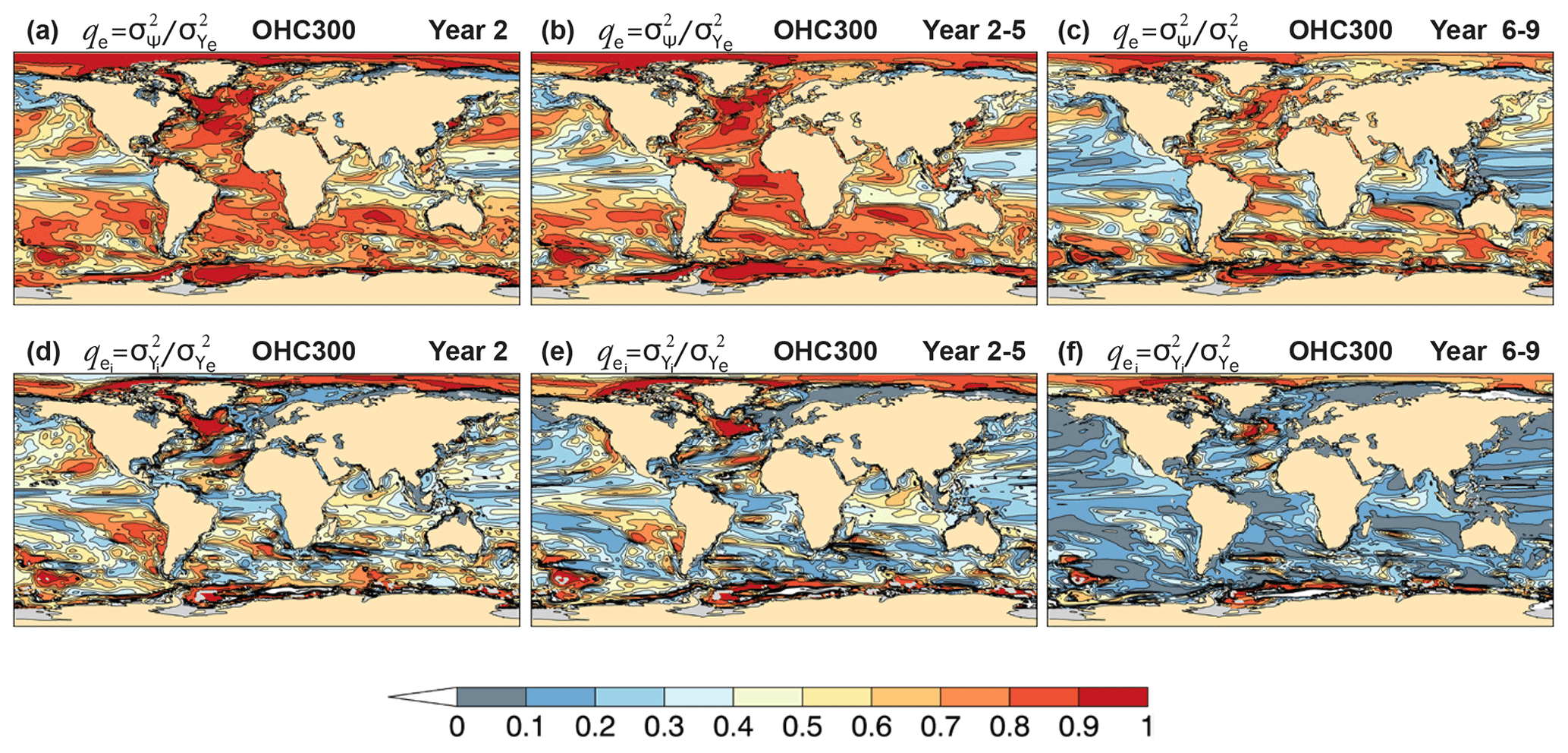
Figure 1Potential predictability of CanESM5 hindcasts of annual and multi-year mean heat content above 300 m. (a–c) Potentially predictable variance fraction , Eq. (4), and (d–f) the portion attributed to initialization for forecast (a, d) Year 2, (b, e) Year 2–5, and (c, f) Year 6–9.
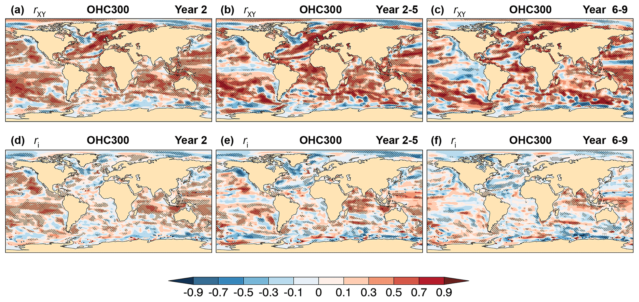
Figure 2Skill of CanESM5 hindcasts of annual and multi-year mean heat content above 300 m. (a–c) Correlation skill rXY, Eq. (6), and (d–f) contribution from initialization ri to correlation skill, Eq. (A17), for forecast (a, d) Year 2, (b, e) Year 2–5, and (c, f) Year 6–9. The verifying observations are derived from the EN4.2.1 data set (Appendix B). Cross-hatched regions indicate values significantly different from zero at the 90 % confidence level.
Some of the predictable variance contributes to skill, but some may reflect model biases and/or initialization errors. The correlation skill rXY of OHC300 hindcasts and the contribution ri from initialization are shown in the upper and lower panels of Fig. 2, respectively. For Year 2, correlation skill is significant over large portions of the global ocean (Fig. 2a) and is reduced in some extratropical regions including sectors of the eastern Pacific, the Arctic and Southern oceans, the Alaskan and western subarctic gyres, and in sectors of the North Atlantic, most notably the western subpolar region (WSPNA) and the Labrador Sea. The negative skill in the WSPNA region is attributed to initialization (Fig. 2d) and is partly a consequence of erroneous trends in ORAS5 reanalysis (Johnson et al., 2019) being imprinted on the hindcasts. The poor skill in the WSPNA and plausible causes are discussed further in Sect. 6 below. Positive contributions from initialization can be seen in large sectors of the Pacific and Indian ocean basins for Year 2, whereas correlation skill in the Atlantic results mostly from uninitialized external forcing (Fig. 2a, d). For multi-year averages (Fig. 2b, c), the geographic extent of positive correlation skill is somewhat reduced relative to Year 2, most notably over the equatorial Pacific and in the Indian basin at longer leads, and tends to increase in magnitude over regions where skill is attributed to the simulated external forcing.
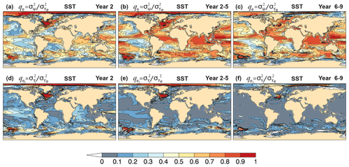
Figure 3Potential predictability of CanESM5 annual mean sea surface temperature hindcasts. (a–c) Potentially predictable variance fraction , Eq. (4), and (d–f) the portion attributed to initialization for forecast (a, d) Year 2, (b, e) Year 2–5, and (c, f) Year 6–9.
Sea surface temperature (SST) hindcasts for Year 2, 2–5, and 6–9 (Fig. 3a–c) show ppvf qe>0.4 in most of the global ocean, with larger values for the multi-year averages. For Year 2, notable contributions from initialization are seen in the western equatorial Pacific, which are not present for the multi-year averages. The predictable SST signal is strongest in the Arctic, in sectors of the Southern Ocean, and in the WSPNA and Labrador Sea regions, resulting entirely from initialization (Fig. 3d–f). These locations are characterized by unrealistic negative trends in the ORAS5 reanalysis (Fig. 4b) that are imprinted in the hindcasts (Fig. 4d) and contribute to the predictable variance attributed to initialization (Fig. 3d–f). On interannual timescales, qe and are generally smaller for SST than OHC300 (Fig. 1a–c), as SST is more directly affected by atmospheric conditions. On multi-year timescales and longer lead times, qe can be larger for SST (Fig. 3c) than OHC300 (Fig. 1c), as the simulated forced component becomes dominant, which strongly impacts SST trends (Fig. 4c).
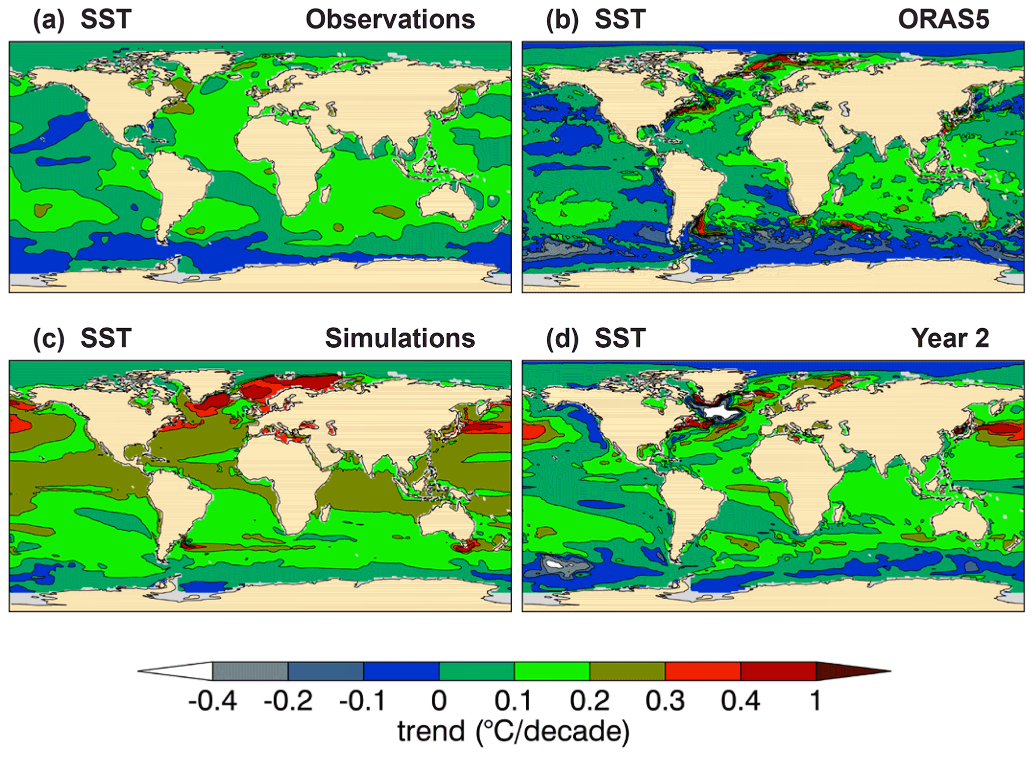
Figure 4Linear trends of annual mean sea surface temperature for (a) observations, (b) ORAS5, (c) uninitialized simulations, and (d) Year 2 hindcasts. The verifying observations are from the ERSSTv5 data set (Appendix B).

Figure 5Skill of CanESM5 annual and multi-year mean sea surface temperature forecasts. (a–c) Correlation skill rXY, Eq. (6), (d–f) contribution from initialization ri to correlation skill, Eq. (A17), and (g–i) correlation skill of the initialized component of the forecast , Eq. (A19), for forecast (a, d, g) Year 2, (b, e, h) Year 2–5, and (c, f, i) Year 6–9. The verifying observations are from the ERSSTv5 data set (Appendix B). Cross-hatched regions indicate values significantly different from zero at the 90 % confidence level.
SST hindcasts show a reasonably widespread correlation skill (Fig. 5a–c). A large fraction of SST correlation skill is attributable to the uninitialized external forcing, but significant contributions ri from initialization are seen in all ocean basins for Year 2 (Fig. 5d) and in sectors of the Pacific and Southern Ocean for the multi-year averages (Fig. 5e–f). The large contribution to skill by the uninitialized component is derived partly from temperature trends that account for a larger variance fraction than that of the initialized component (Fig. 3), which is itself skillful as per (Fig. 5g–i). This shows that despite the significant correlation skill of the initialized component Yi, the associated small variance fraction (Fig. 3) reduces the contribution (Eqs. 5 and 6) of the initialized component to correlation skill. The apparent skill re-emergence of the initialized component in the eastern Pacific for Year 6–9 is noteworthy (Fig. 5i).
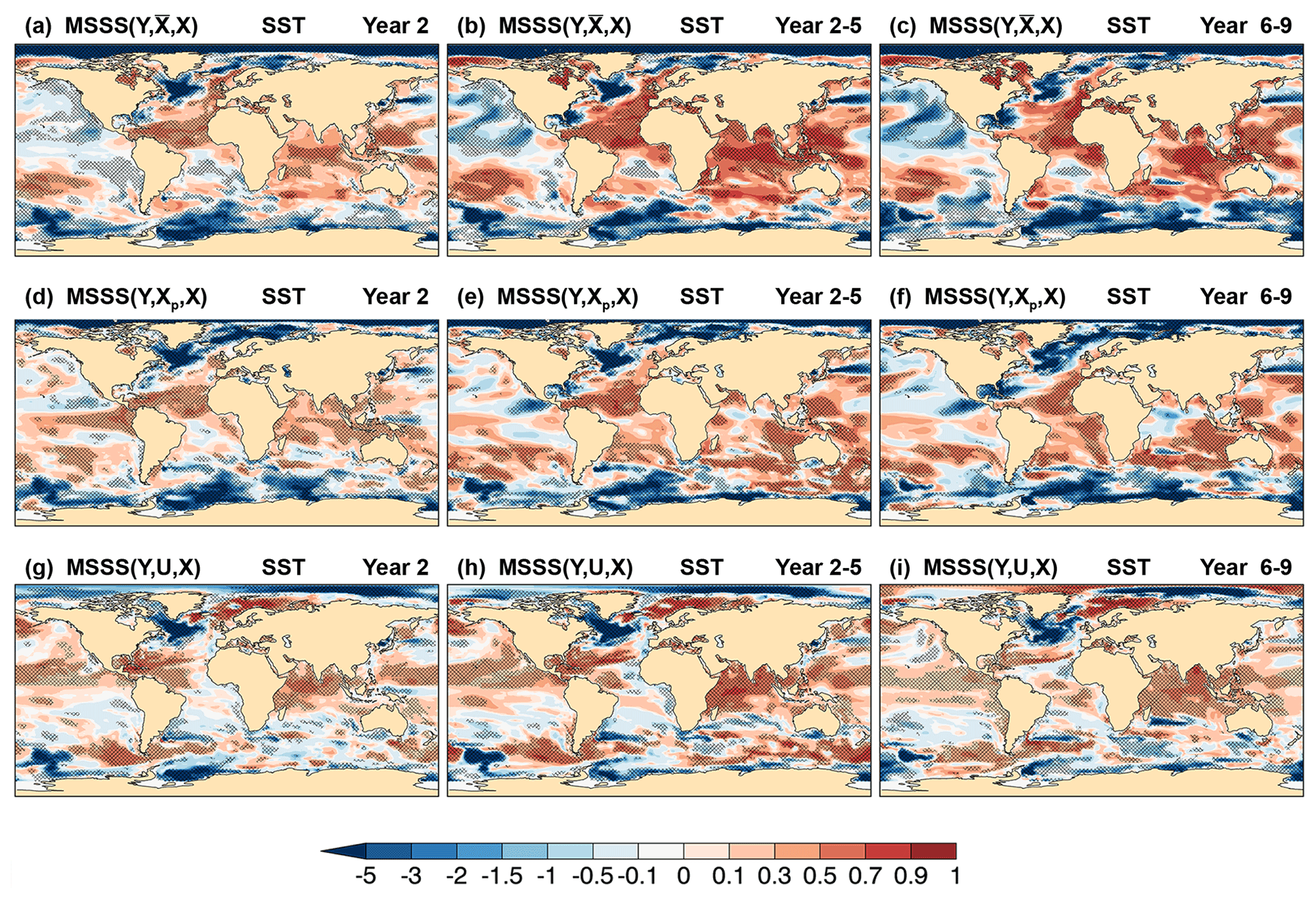
Figure 6Skill of CanESM5 annual and multi-year mean sea surface temperature hindcasts. MSSS of (a, d, g) Year 2, (b, e, h) Year 2–5, and (c, f, i) Year 6–9 hindcasts, Y, relative to (a–c) observed climatology, , (d–f) persistence forecast, Xp, and (g–i) uninitialized simulations, U. The verifying observations are from the ERSSTv5 data set (Appendix B). Cross-hatched regions indicate values significantly different from zero at the 90 % confidence level.
MSSS of SST hindcasts relative to observed climatology (Fig. 6a–c) indicates significant skill in large sectors of the North Atlantic, in the Indian Ocean, and in the western Pacific extending into the southeast extratropics. MSSS is a more stringent measure than correlation skill, and regions with significant correlation skill but near-zero or negative MSSS indicate a misrepresentation of the observed variance for the given linear relationship between predictions and observations (i.e., due to a conditional bias). This is the case for various extratropical regions and sectors of the tropical Pacific (compare Figs. 5a–c and 6a–c). Regions with MSSS ≪ 0 indicate a disproportionally large predicted variance relative to observations, such as in WSPNA and Labrador Sea, the Arctic, and the Southern Ocean (Fig. 6a–c). These regions are characterized by high qe (Fig. 3a–c) with a strong impact from initialization (Fig. 3d–f) but lack actual skill (Figs. 5a–c and 6a–c). For Year 2, SST hindcasts outperform persistence in most of the tropics (Fig. 6d), except for sectors of the subequatorial and western Pacific, and the western South Atlantic. For the multi-year averages (Fig. 6e, f), SST hindcasts beat persistence in large sectors of the Atlantic and Indian oceans, and in most western and southern portions of the Pacific within the 40∘ S–40∘ N latitude band. The hindcasts outperform the uninitialized simulations, particularly for multi-year averages (Fig. 6h, i), in vast subequatorial regions, in the Indian Ocean, and in northern and subpolar regions, but underperform in sectors of the Southern Ocean, the eastern and southern Atlantic, and in the WSPNA and Labrador Sea regions.
The negative correlation skill in the WSPNA and Labrador Sea for both upper-ocean heat content (Fig. 2) and SST (Fig. 5) is fully attributed to initialization (i.e., rXY=ri), indicating a mismatch between the external forced response in the hindcasts and uninitialized simulations (SB20), which can be different, as implied by Eq. (1). CanESM5 ocean is initialized with ORAS5 (Sect. 3), which has unrealistic temperature and salinity trends in the upper subpolar North Atlantic associated with erroneous water mass and heat transport before the 2000s (Jackson et al., 2019; Tietsche et al., 2020). The Labrador Sea in ORAS5 presents large changes in density anomaly, most notably in deep waters (1500–1900 m), which decrease abruptly from the late 1990s to the early 2000s, leading also to unobserved trends (Fig. 9 of Jackson et al., 2019). These variations and unrealistic trends are imprinted on CanESM5 assimilation runs as they are nudged toward ORAS5 temperature and salinity fields to initialize the hindcasts (Sect. 3). The anomalous heat and saline surface water transport into WSPNA is largely compensated in ORAS5 by a strong surface cooling provided by relaxation to observed SST (Tietsche et al., 2020), but such a cooling is not present in the forecasts, which leads to imbalances. This, combined with the model inherent biases in the region (S19) and resulting forecast drift, yields unrealistic decadal variations and long-term trends in the hindcasts themselves, which affect skill.
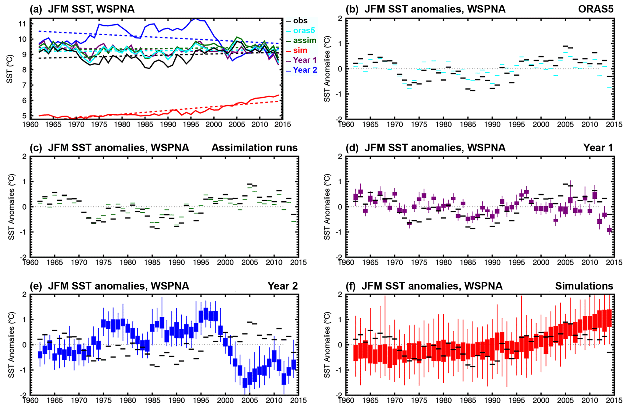
Figure 7JFM time series of (a) SST and (b–f) SST anomalies corresponding to (black) ERSSTv5, (cyan) ORAS5, and CanESM5 (green) assimilation runs, (purple) Year 1 and (blue) Year 2 hindcasts, and (red) uninitialized simulations, averaged over the WSPNA region (40–60∘ N, 50–30∘ W). Boxes and whiskers indicate the minimum, maximum, 25th and 75th percentiles of the 40-member CanESM5 ensemble of forecasts and simulations, and the first 10-member ensemble for the assimilation runs. Model values in (a) correspond to ensemble means and dashed lines represent linear trends. Trends are not removed from the anomalies in (b)–(f).

Figure 7a shows January–February–March (JFM) time series and linear trends of SST averages over WSPNA (40–60∘ N, 50–30∘ W) for ERSSTv5 as verifying observations, ORAS5, and CanESM5 assimilation runs, Year 1 and Year 2 hindcasts, and the uninitialized simulations. Analogous plots for averages over the Labrador Sea (55–65∘ N, 60–45∘ W) are shown in Fig. 8. In WSPNA, ORAS5 is warmer than observations during the mid-1970s to about the 2000s, as is the case for the assimilation runs. Year 1 hindcasts remain close to initial SST for most years, although they are somewhat colder during the late 1990s and onward. Year 2 SST hindcasts, on the other hand, have a strong warming in the early 1970s and remain 2–3 ∘C warmer than observations until the late 1990s, when a steep cooling occurs to below observed values until the early 2000s. These changes yield a negative trend for Year 2 hindcasts (−0.02 ∘C per decade) that does not match the slight warming trend from observations (0.01 ∘C per decade). By comparison, ORAS5 and the assimilation runs have virtually no trend, with values of 0.002 and 0.004 ∘C per decade, respectively. For longer lead times, the hindcasts drift toward simulations (not shown), which are characterized by a strong cold bias (−3.65 ∘C) and a warming trend (0.03 ∘C per decade) described in some detail in S19 (see Figs. 15a, b and 26 of S19).
JFM time series of SST anomalies averaged over WSPNA are shown in Fig. 7b–f. The observed anomalies present distinctive decadal variations, with warm phases before 1970 and from the late 1990s until about 2010, and a cold phase between 1970 and the early 1990s. These decadal variations are modestly represented by ORAS5 (r=0.77 and RMSE = 0.28 ∘C, Fig. 7b), which has weaker and out-of-phase anomalies, and are better represented by the assimilation runs (r=0.94 and RMSE = 0.16 ∘C for the ensemble mean, Fig. 7c). Year 1 hindcasts perform modestly (r=0.43 and RMSE = 0.42 ∘C, Fig. 7d), and Year 2 hindcasts poorly, showing strong decadal variations that are mostly out of phase with observations ( and RMSE = 1.04 ∘C, Fig. 7e). The anomalies of the simulations, which are characterized by a warming trend, are not expected to match the internally generated variability of the observed anomalies (r=0.42 and RMSE = 0.46 ∘C, Fig. 7f), although the latter are mostly contained within the ensemble spread. Analogous plots for the Labrador Sea (Fig. 8b–f) show disagreement also between ORAS5 and observed JFM SST anomalies, as well as for the assimilation runs, which are imprinted in the forecasts leading to unrealistic strong and out-of-phase variations for Year 2. The simulation ensemble presents anomalies above −0.2 ∘C during the whole time period which are virtually unchanged in the mean at subzero temperatures prior to the year 2000 as a result of excessive sea ice (S19). The poor skill in WSPNA and the Labrador Sea are likely to impact predictions of surface climate over North America and Europe (Eade et al., 2012; Ruprich-Robert et al., 2017a), and west Africa and the Sahel (Martin and Thorncroft, 2014b; García-Serrano et al., 2015). Predictability of the tropical Atlantic (Dunstone et al., 2011), ocean heat content in the Nordic Seas, and decadal Arctic winter sea ice trends (Yeager and Robson, 2017) could also be affected.
One of the main motivations for decadal climate prediction is the understanding that low-frequency variations in the upper-ocean heat content can influence surface climate by inducing atmospheric circulation changes both locally and remotely (Zhang and Delworth, 2006; Ruprich-Robert et al., 2017b). The expectation is that ocean model initialization will allow skillful surface climate prediction from seasons to years (Smith et al., 2007; Doblas-Reyes et al., 2011). Assessing the influence of model initialization on forecast skill can be challenging however (Smith et al., 2019), particularly in the presence of strong secular trends that can hinder the detection of internally generated predictable variations. Meehl et al. (2020) report that CanESM5 has equilibrium climate sensitivity (ECS) and transient climate response (TCR) at or near the top of the range among the Earth system models participating in CMIP6, with ECS = 5.6 K in the 1.8 to 5.6 K range, and TCR = 2.7 K in the 1.3 to 3.0 K range. CanESM5 also exhibits a strong historical warming trend (Figs. 25a and 26, S19), which leads to global temperatures changes exceeding those observed toward the end of the historical period, especially over the Arctic and on land regions. Therefore, improvement of forecast skill in CanESM5 SAT predictions over land can be expected due to the impact of initialization not only on internally generated variability but also on corrections to this excessive warming trend.
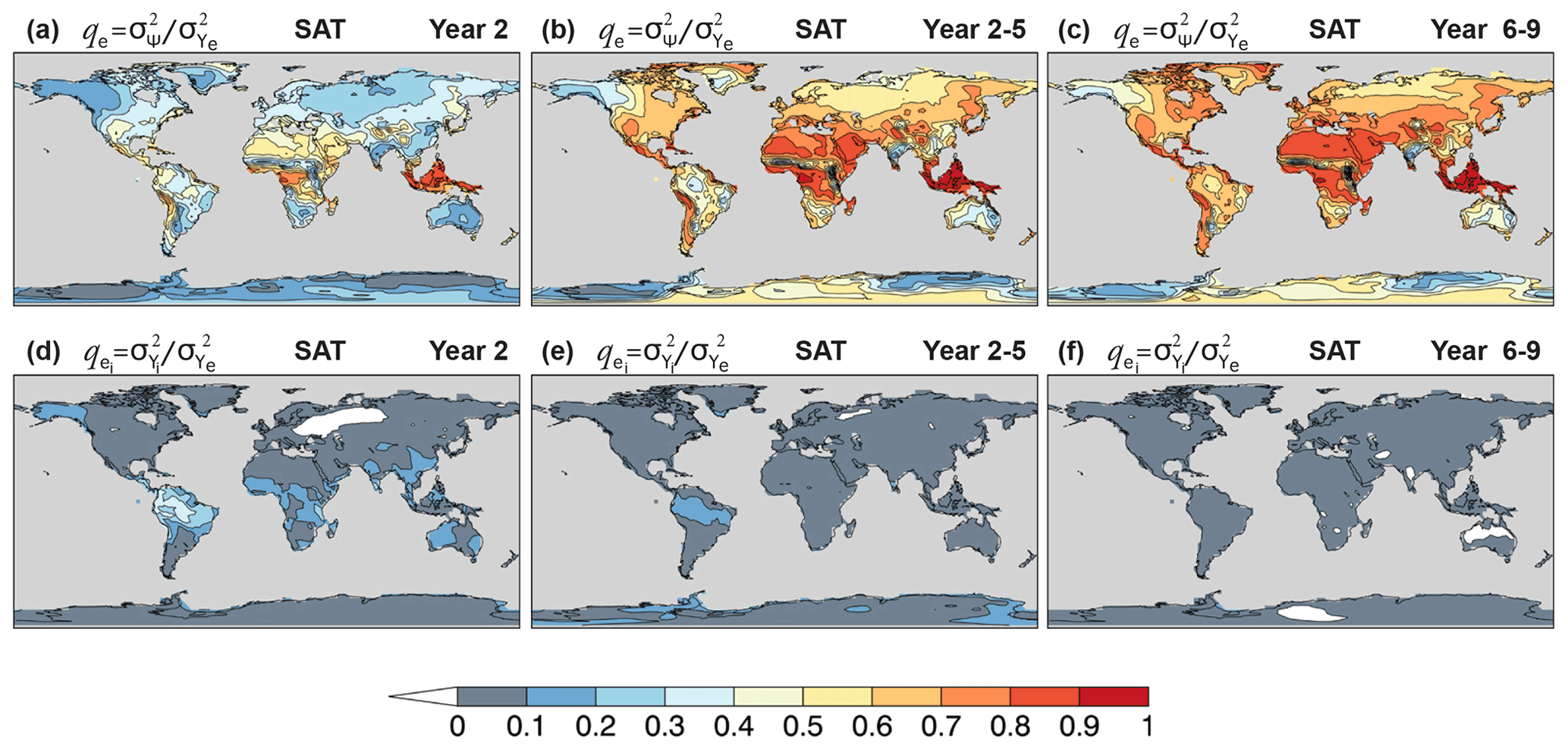
Figure 9Potential predictability of CanESM5 annual and multi-year mean near-surface air temperature hindcasts. (a–c) Potentially predictable variance fraction , Eq. (4), and (d–f) the portion attributed to initialization for forecast (a, d) Year 2, (b, e) Year 2–5, and (c, f) Year 6–9.
Figure 9a–c show qe of annual mean near-surface air temperature (SAT) on land for Year 2, Year 2–5, and Year 6–9 hindcasts. For Year 2, the ppvf is generally largest in the tropics (qe>0.4), where atmospheric circulation is most strongly influenced by SST (Lindzen and Nigam, 1987; Smith et al., 2012). Tropical regions are impacted by initialization (), most notably in the Amazon, where to 0.4 (Fig. 9d). Extratropical regions are characterized by a relatively higher atmospheric noise, thus displaying reduced ppvf (qe<0.4) and little contribution from initialization. For multi-year averages, the noise component is reduced considerably, leading to a relatively high ppvf (Fig. 9b, c), particularly in regions were the warming trend is dominant (Fig. 10). The impact of initialization is also reduced, with typically (Fig. 9e, f).
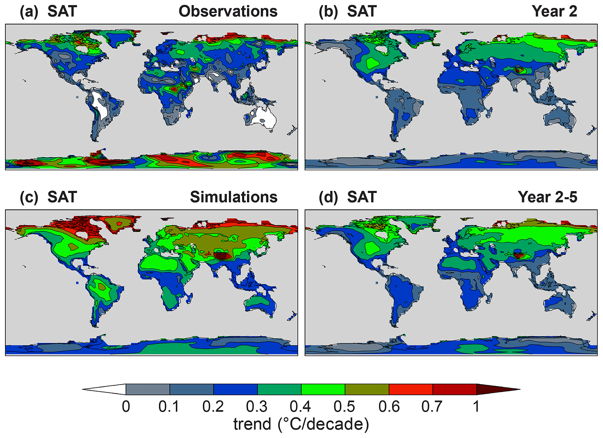
Figure 10Decadal trends of annual mean near-surface air temperature for (a) observations, (b) Year 2 and (d) Year 2–5 hindcasts, and (c) uninitialized simulations. The verifying observations are from the ERA-40 and ERA-Interim data sets (Appendix B).

Figure 11Skill of CanESM5 annual and multi-year mean near-surface air temperature hindcasts. MSSS of (a, d, g) Year 2, (b, e, h) Year 2–5, and (c, f, i) Year 6–9 hindcasts, Y, relative to (a–c) observed climatology, , (d–f) persistence forecast, Xp, and (g–i) uninitialized simulations, U. The verifying observations are from the ERA-40 and ERA-Interim data sets (Appendix B). Cross-hatched regions indicate values significantly different from zero at the 90 % confidence level.
SB20 show that annual and multi-year averages of CanESM5 SAT hindcasts have significant correlation skill over most land regions due to the strong temperature response to external forcing, with a modest contribution from initialization. In terms of MSSS, SAT hindcasts on land are more skillful than observed climatology (MSSS > 0) in the tropics and in regions near large water masses (Fig. 11a–c), mirroring the behavior of qe in Fig. 9a–c. Skill is highest for multi-year averages, where significant MSSS values are also seen inland (Fig. 11b, c). Notably, MSSS < 0 in the Amazon in spite of positive correlation skill (Fig. 3 of SB20), indicating an excessive variance in the hindcasts possibly due to unrealistic trends (Fig. 10). The hindcasts outperform persistence in the extratropics but underperform in the tropics most notably in Year 2 (Fig. 11d), primarily over regions of unrealistic trends (Fig. 10). By contrast, the hindcasts outperform simulations in the tropics (Fig. 11g) where initialization contributes to ppvf (Fig. 9d) and correlation skill (Fig. 3e of SB20), except for central Africa and the Sahel. For multi-year averages, the hindcasts outperform simulations in most regions (Fig. 11h, i), despite little impact from initialization to correlation skill (Fig. 3f of SB20), suggesting that the improvements are likely due to reductions of the simulated trends (Fig. 10).
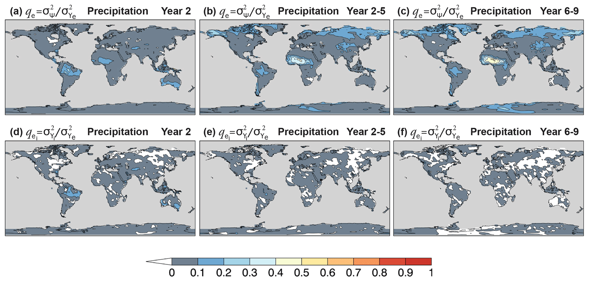
Figure 12Potential predictability of CanESM5 annual and multi-year precipitation hindcasts. (a–c) Potentially predictable variance fraction , Eq. (4), and (d–f) the portion attributed to initialization for forecast (a, d) Year 2, (b, e) Year 2–5, and (c, f) Year 6–9.
The upper panels of Fig. 12 show qe of annual mean precipitation hindcasts for Year 2, Year 2–5, and Year 6–9. For Year 2, qe>0.1 is confined to tropical and subtropical regions, with slightly higher values in the Amazon basin (). The precipitation signal extends to higher latitudes and is relatively stronger for multi-year averages. The largest ppvf values are seen in the Sahel for longer lead times (qe>0.5 for Year 6–9 in some locations) as the externally forced component becomes dominant. Generally, most of the hindcast precipitation signal with qe>0.1 is externally forced. The largest contributions of initialization to ppvf are seen in northeastern Brazil, central southwestern Asia, and southern Australia for Year 2 hindcasts (), and elsewhere (Fig. 12d–f). The negative values of seen in the plots are the result of a negligible impact from initialization and sampling errors. Sources of the predictable signal and prediction skill in northeastern Brazil, central southwestern Asia, and the Sahel are discussed in Sect. 8.

Figure 13Skill of CanESM5 annual and multi-year mean precipitation hindcasts. (a–c) Correlation skill rXY, Eq. (6), and (d–f) contribution from initialization ri to correlation skill, Eq. (A17), for forecast (a, d) Year 2, (b, e) Year 2–5, and (c, f) Year 6–9. The verifying observations are from the GPCP2.3 data set (Appendix B). Cross-hatched regions indicate values significantly different from zero at the 90 % confidence level.
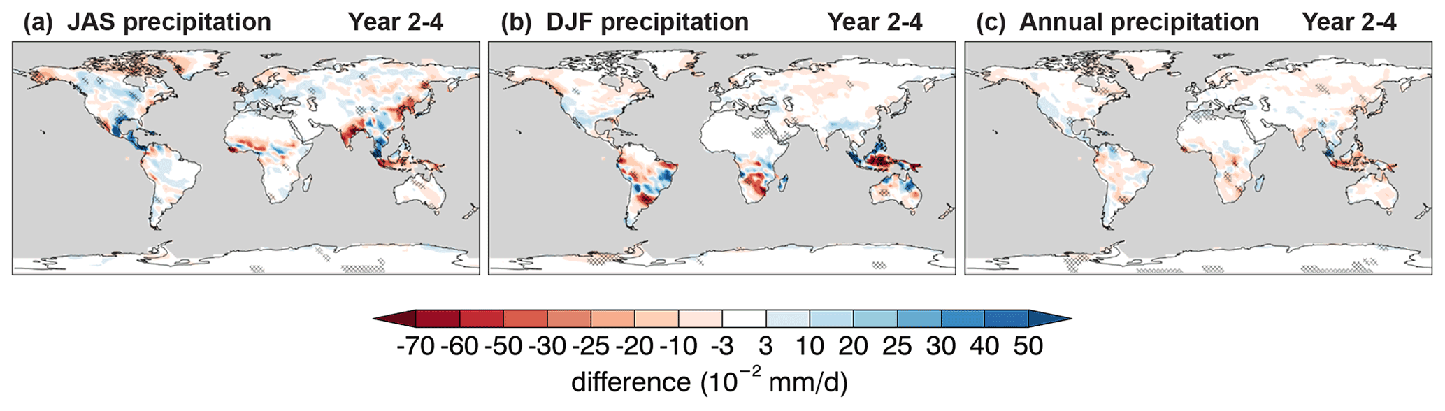
Figure 14The impact of volcanic aerosols on mean precipitation forecasts. Difference of (a) summer (July–August–September), (b) winter (December–January–February), and (c) annual mean Year 2–4 precipitation forecasts with and without volcanic eruptions. Computations include 10-member ensembles of forecasts with and without eruptions of Mount Agung, El Chichón, and Mount Pinatubo as per the DCPP Component C volcanic experiment setup (Boer et al., 2016). Cross-hatched regions indicate values significantly different from zero at the 90 % confidence level.
The correlation skill of the annual mean precipitation hindcasts (Fig. 13a–c) partly mirrors the patterns of Fig. 12a–c but can be significant also in regions of low ppvf. Correlation skill tends to increase both in magnitude and geographic extent for multi-year averages (Fig. 13b, c). A large component of skill is attributed to the uninitialized forced component, as can be inferred from Fig. 13d–f. Known sources of externally forced decadal precipitation variability include drivers of climate change such as CO2 and anthropogenic SO2, which can alter the energy budget due to changes in the atmospheric composition, leading to climate feedback processes that affect precipitation (Myhre et al., 2017). Another major source is volcanic aerosols, which are injected into the stratosphere during a volcanic eruption and can reduce global mean temperature leading to a drier atmosphere and reduced precipitation 2 to 3 years after an event (Smith et al., 2012). This is shown in Fig. 14 by the difference of mean precipitation from hindcasts with and without volcanic forcing following three major volcanic events (Agung, 1963; El Chichón, 1982; and Pinatubo, 1991). The setup of these volcanic experiments is briefly described in Sect. 3 and follows the recommendations of Boer et al. (2016) as part of Component C of the DCPP. The difference in mean precipitation is significant over various land regions and most notably in the Maritime Continent. Precipitation hindcasts over this region have significant correlation skill (Fig. 13a–c) not fully associated with initialization (Fig. 13d–f); thus, volcanic forcing could be a contributing factor. Contributions from initialization to correlation skill are significant in a few regions including northeastern Brazil, western North America, and central southwestern Asia for Year 2 and Year 2–5 (Fig. 13d, e), and are much reduced for Year 6–9 (Fig. 13f).
Large single- and multi-model ensembles of initialized and uninitialized predictions have become essential tools in the study of decadal climate predictions due in part to the considerable noise reduction that can be achieved by ensemble averaging (Yeager et al., 2018; Deser et al., 2020; Smith et al., 2020). Generally, the ensemble size required to extract predictable signals varies among climatic variables and may depend on forecast range, in the case of initialized predictions, and on geographic location. The tendency for models to underestimate predictable signals (Scaife and Smith, 2018; Smith et al., 2020) reinforces the need for large ensembles.
Figure 15 shows the noise-to-predictable-variance ratio γY, Eq. (A12), and γU, Eq. (A13), of annual and multi-year mean terrestrial precipitation for the 40-member ensembles of hindcasts and uninitialized simulations. The global land averages of γY and γU as a function of ensemble size stabilize for ≳10 members (not shown), suggesting that the patterns of Fig. 15 are largely robust under changes in ensemble samples and sizes. In terms of , the ensemble size required for q>q0 is, according to Eq. (5), , so requires mY>9γY. Therefore, all regions in Fig. 15a, b with, say, γY>5 require mY>45 members to satisfy q>0.9, i.e., over 45 members are needed for the variance of the ensemble mean hindcast to be at least 90 % predictable. Most regions in Fig. 15a, b have γY>5, suggesting a benefit of large ensembles. A few exceptions include the Amazon basin for interannual variations (Fig. 15a) and the Sahel for multi-year variations (Fig. 15b), which are both characterized by relatively strong precipitation signals. A similar analysis can be made for the uninitialized simulations.
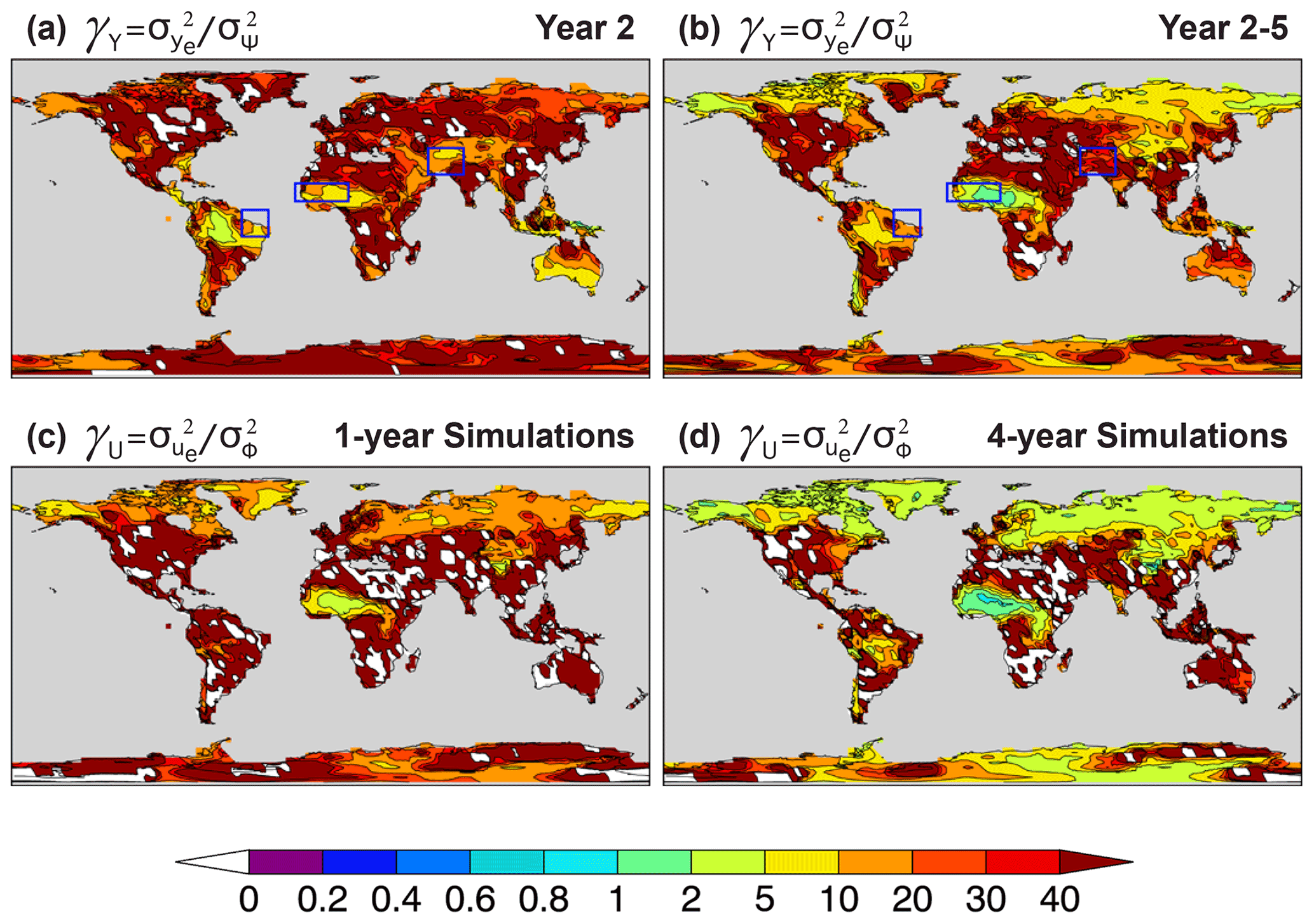
Figure 15Maps of noise-to-predictable-variance ratio (a, b) γY, Eq. (A12), for (a) Year 2 and (b) Year 2–5 hindcasts and (c, d) γU, Eq. (A13), for (c) 1-year and (d) 4-year averaged uninitialized simulations of annual mean precipitation. The γY ratio determines the ensemble size required to average out the noise component from the ensemble mean forecast, Eq. (5), and similarly γU for simulations. Negative values (white on land) result from sample errors, indicating small ensemble mean variance, and therefore a small predictable signal, relative to the noise variance. The maps are produced with the full 40-member ensembles of hindcasts and uninitialized simulations. Rectangular boxes indicate the regions studied in Figs. 16–18 below.
To illustrate forecast skill dependence on ensemble size, precipitation predictions over northeastern Brazil (NEB; 10∘ S–5∘ N, 50–35∘ W) and central southwestern (CSW) Asia (25–55∘ N, 40–75∘ E) are considered. These two regions stand out for the potentially predictable precipitation signal (Fig. 15a, b) and associated correlation skill due to initialization (Fig. 13a, d). Precipitation variability over NEB has been linked to variations of the intertropical convergence zone modulated by Atlantic SST gradients and tropical Pacific SST anomalies, the latter mainly driven by El Niño–Southern Oscillation on interannual timescales, which are in turn modulated by the Atlantic Multidecadal Variability and the Interdecadal Pacific Oscillation on decadal timescales (Nobre et al., 2005; Villamayor et al., 2018). Over CSW Asia, wintertime precipitation anomalies have been linked to variations of the East Asian jet stream driven partly by western Pacific convection and SST anomalies, and Maritime Continent convection (Barlow et al., 2002; Tippett et al., 2003).
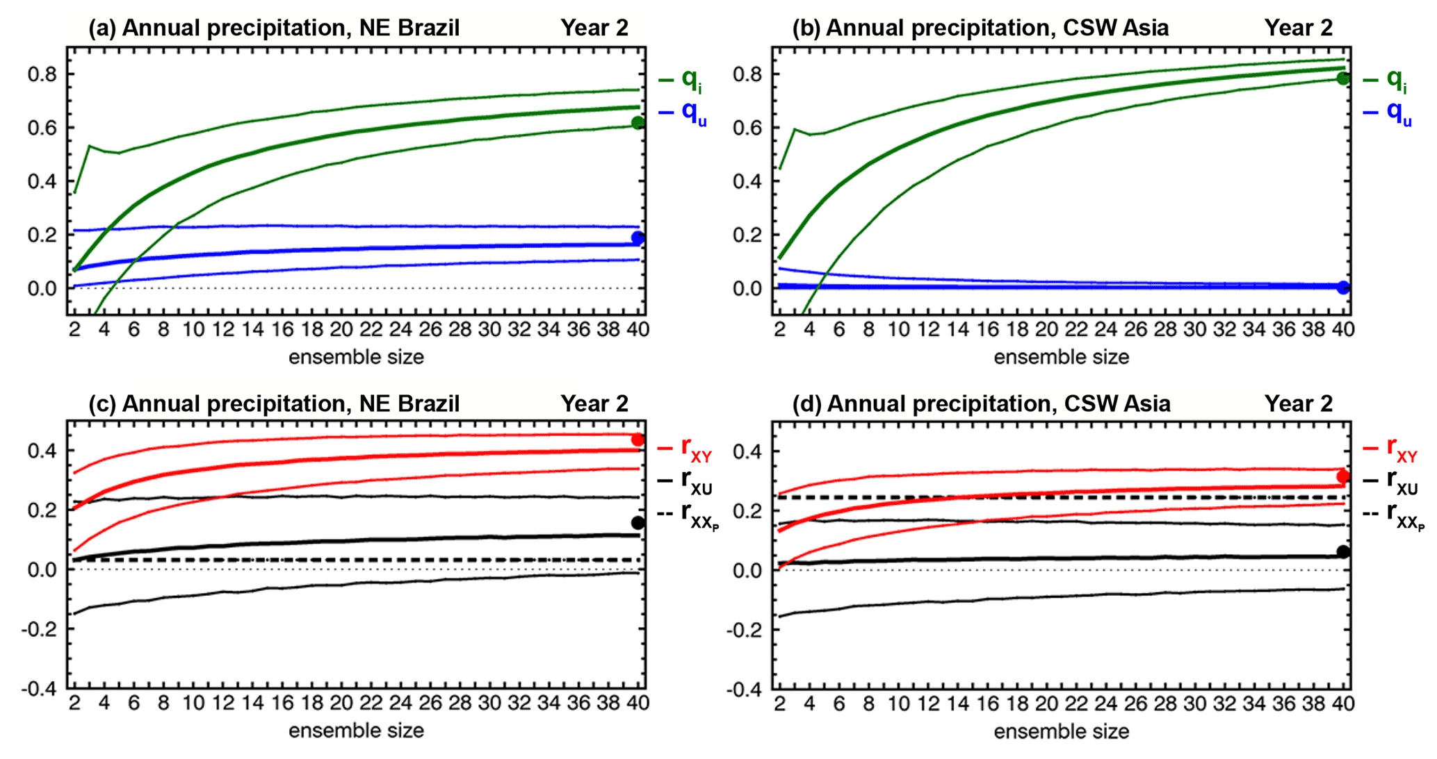
Figure 16Dependence on ensemble size of (a, b) variance contributions , Eq. (A14), in blue, and , Eq. (A15), in green, to (c, d) correlation skill rXY, Eq. (6), in red, of Year 2 ensemble mean precipitation hindcasts, averaged over (a, c) northeastern Brazil (−10–5∘ N, 50–35∘ W) and (b, d) central southwestern Asia (25–55∘ N, 40–75∘ E). These regions are highlighted in Fig. 15 above. Thick black curves indicate correlation skill rXU of ensemble mean uninitialized simulations. Thick dashed lines indicate correlation skill of the persistence forecast. Thin curves are confidence intervals derived from the 5th and 95th percentiles of bootstrapping distributions generated from 10 000 samples by random selection, with replacement, of ensemble members for each indicated ensemble size. Filled dots correspond to the actual 40-member ensemble predictions. Computations of qu, Eq. (A14), and qi, Eq. (A15), are done with mY=2…40 members from the hindcast ensemble and, for each mY, the 40 members from the uninitialized simulations ensemble. The verifying observations used to compute correlation skill are from the GPCP2.3 data set (Appendix B).
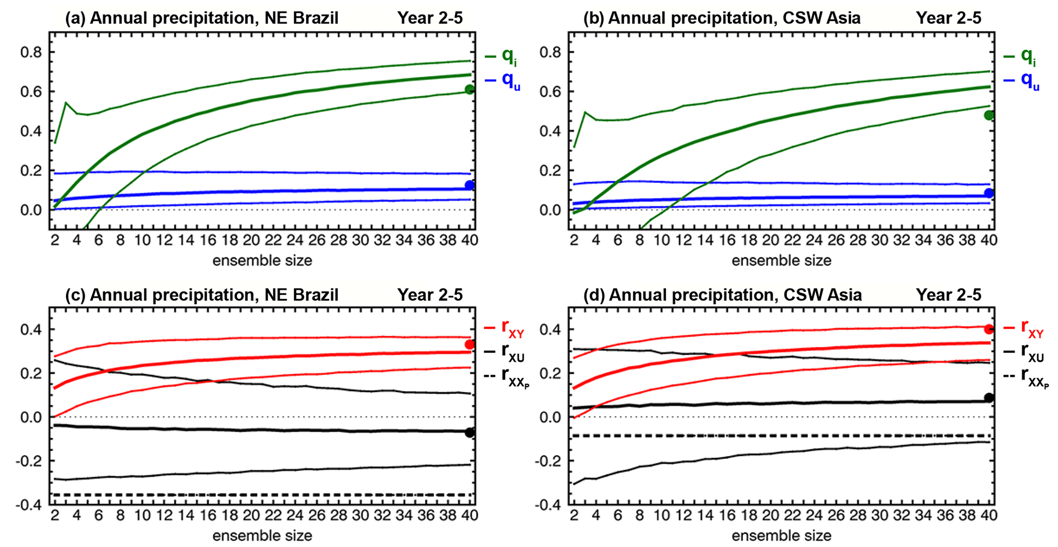
Figure 16a, b show the dependence on ensemble size of the variance contributions and to correlation skill rXY from the uninitialized Yu and initialized Yi components of Year 2 annual mean precipitation hindcasts averaged over NEB and CSW Asia. For both regions, qu≲0.2 for all ensemble sizes, indicating small variance contribution to skill from the simulated response to external forcing. By contrast, qi increases from about 0.40 for ensemble size mY=10 to about 0.65 for mY=40 over NEB, and from about 0.50 for mY=10 to about 0.80 for mY=40 over CSW Asia, showing that initialization impacts the ppvf in Eq. (5), and that large ensembles are required to extract the initialized predictable variance from the ensemble mean hindcast. The variance contribution to correlation skill will increase further, albeit minimally and slowly, for ensemble sizes larger than 40, so there is a limit to the cost-effective increase of ensemble size to improve skill. For Year 2–5, the behavior is somewhat similar (Fig. 17a, b), although the variance contribution of the initialized (uninitialized) component tends to be lower (higher).
Besides their variance contribution to skill, Yu and/or Yi must have realistic variations in phase for a skillful ensemble mean prediction Y. The correlation skill rXY for the Year 2 annual mean precipitation hindcast averaged over NEB and CSW Asia is shown in Fig. 16c, d as a function of ensemble size. Also shown are the correlation skills rXU of the uninitialized simulations and of the persistence forecast. For both regions, the hindcast correlation skill is positive at the 90 % confidence level. Hindcast skill increases with ensemble size and surpasses that of uninitialized simulations for mY≳15, indicating an added value from initialization that would have been underestimated for mY<15 by this metric. Unlike uninitialized simulations, the hindcasts over NEB are more skillful than persistence for all ensemble sizes (Fig. 16c). By contrast, the median correlation skill over CSW Asia surpasses persistence for mY≳20 but may require more than 40 members to do so confidently (Fig. 16d). It should be noted, however, that forecast correlation skill is higher when averaged over winter and spring (DJFMAM), and surpasses that of persistence and of the simulations for mY>10 (not shown). This is consistent with the seasonal cycle of mean precipitation over CSW Asia (Tippett et al., 2003; Schiemann et al., 2008), as the precipitation signal is stronger during DJFMAM. For Year 2–5 (Fig. 17c, d), the hindcasts over NEB are more skillful than uninitialized simulations for mY≳20 but require mY≳35 to marginally outperform simulations over CSW Asia, indicating an advantage of large ensembles.

Figure 18Dependence on ensemble size of (a, b) correlation skill of ensemble mean forecasts rXY (red) and ensemble mean simulations rXU (black); (c, d) contributions ru, Eq. (A16), in royal blue, and ri, Eq. (A17), in olive, to rXY; and (e, f) ratio Πr, Eq. (8), of hindcasts (salmon) and uninitialized simulations (gray), for (a, c, e) Year 2 and (b, d, f) Year 2–5 precipitation hindcasts, averaged over the Sahel (10–20∘ N, 20∘ W–10∘ E). This region is highlighted in Fig. 15 above. Thick dashed lines indicate correlation skill of the persistence forecast. Thin curves are confidence intervals derived from the 5th and 95th percentiles of bootstrapping distributions generated from 10 000 samples by random selection, with replacement, of ensemble members for each indicated ensemble size. Filled dots correspond to the actual 40-member ensemble predictions. Computations of ru, Eq. (A16), and ri, Eq. (A17), are done with mY=2…40 members from the hindcast ensemble and, for each mY, the 40 members from the uninitialized simulations ensemble. The verifying observations used to compute correlation skill are from the GPCP2.3 data set (Appendix B).
The results over the Sahel are somewhat different. The Sahel is an important benchmark for the assessment of decadal predictions due to its strong summer rainy season, the variation of which is considered one of the largest signals of global climatic variability on annual to multi-year timescales (Martin and Thorncroft, 2014a; Sheen et al., 2017). Previous studies indicate that initialization enhances the skill of Sahelian rainfall predictions compared to simulations, although results vary among models (Garcia-Serrano et al., 2013; Gaetani and Mohino, 2013; Martin and Thorncroft, 2014a; Sheen et al., 2017; Yeager et al., 2018). Figure 18a, b show the dependence on ensemble size of Year 2 and Year 2–5 forecast correlation skill rXY for July–August–September (JAS) mean precipitation averaged over the Sahelian sector (10–20∘ N, 20∘ W–10∘ E), as well as rXU and for the uninitialized simulations and persistence, respectively. Generally, hindcasts and uninitialized simulations outperform persistence by a large margin, but both exhibit about the same level of skill, suggesting virtually no impact from initialization. The increase in skill is accompanied by a reduction in skill uncertainty, illustrating a benefit of large ensembles. The correlation skill decomposition indicates that the externally forced component is the main contributor to forecast skill with a negligible impact from initialization (Fig. 18c, d).
The small impact of initialization on Sahelian rainfall hindcasts is at odds with previous findings (Gaetani and Mohino, 2013; Yeager et al., 2018). Interannual and multidecadal variability of Sahelian rainfall has been linked to SST variability in the global ocean (Rowell et al., 1995), the Atlantic (Ward, 1998; Knight et al., 2006; Zhang and Delworth, 2006; Ting et al., 2009; Martin and Thorncroft, 2014a, b; Yeager et al., 2018), the Pacific and Indian oceans (Mohino et al., 2011b; Sheen et al., 2017), and the Mediterranean Sea (Rowell, 2003; Mohino et al., 2011a; Sheen et al., 2017). Greenhouse gases and aerosols have also been linked to decadal variability and trends of Sahelian rainfall by their impact on Atlantic interhemispheric SST gradients and resulting effect on the intertropical convergence zone (Biasutti and Giannini, 2006; Haywood et al., 2013; Hua et al., 2019; Bonfils et al., 2020) and by a direct effect of changes in radiative forcing (Haarsma et al., 2005; Biasutti, 2013; Dong and Sutton, 2015). Despite the negligible impact from initialization, CanESM5 precipitation skill over the Sahel is relatively high, particularly for Year 2–5 (rXY≈0.7, Fig. 18b) and other multi-year averages (not shown), and comparable to the skill of CMIP5/6 decadal predictions from other models (Gaetani and Mohino, 2013; Yeager et al., 2018). This may be an indication that at least part of the enhanced forecast prediction skill of Sahelian rainfall in some CMIP5/6 models relative to that of uninitialized simulations might be a consequence of the impact of initialization on the forced component rather than a skillful prediction of the internally generated variability itself (i.e., due to the term in parenthesis in the definition of Yi in Eq. 3).
The ratio Πr, Eq. (8), for the Sahelian JAS mean precipitation hindcasts increases with ensemble size and confidently surpasses 1 with 40 members for Year 2 (Fig. 18e) and approximately 15 members for Year 2–5 (Fig. 18f), indicating that for larger ensembles rXY>ρ; i.e., the ensemble mean hindcast is more skillful at predicting the observed climate system than the hindcasts themselves. This is a consequence of the noise-to-predictable-variance fraction γY being too high, suggesting that the hindcasts are either too noisy or their predictable components are too weak relative to the observed precipitation signal. Because the hindcasts and observed total JAS precipitation variances are about the same (not shown), we conclude that the ensemble mean hindcast underestimates the amplitude of the predictable precipitation signal in the Sahel. A similar behavior is seen for the uninitialized simulations with a somewhat reduced predictable variance fraction for large ensembles, particularly for Year 2–5 (Fig. 18f), which is primarily a consequence of the stronger potentially predictable variance of the simulations (not shown). Such behavior is not specific to CanESM5 nor to the region, climate variable, and timescales involved. It is a feature across model simulations of various climate phenomena (Scaife and Smith, 2018; Yeager et al., 2018; Smith et al., 2020), pointing to model deficiencies at representing the strength of predictable signals of the climate system.
CanESM5 models the effects of the physical climate on the biosphere and the chemical constituents of the atmosphere and ocean. This enables the assessment of some aspects of the predictability of ocean and land biogeochemistry, and the carbon cycle. Gross primary productivity (GPP) is the rate of photosynthetic carbon fixation by primary producers, such as phytoplankton in the ocean and plants on land. GPP of terrestrial vegetation is a key variable of the global carbon cycle and is an important component of climate change (Zhang et al., 2017). Net primary productivity (NPP) is the difference between GPP and the fraction of fixed carbon that primary producers use for respiration (Gough, 2011; Sigman and Hain, 2012) and is thus a major determinant of carbon sinks and a key regulator of ecological processes (Field et al., 1998). The potential for predictive skill of NPP hindcasts in the ocean and GPP hindcasts on land is assessed here by correlation with the assimilation runs used for initialization. We also show preliminary comparisons with observation-based estimates but do not provide a full assessment of actual skill due to the relatively short time span of the observations. As in previous sections, uninitialized simulations are used here as a reference to quantify the impact of initialization on hindcast correlation skill. We emphasize that there is no assimilation of observed carbon cycle variables to initialize the hindcasts (Sect. 3); therefore, initial variations of GPP and NPP are the result of ensemble spread of oceanic and atmospheric states in the assimilation runs.
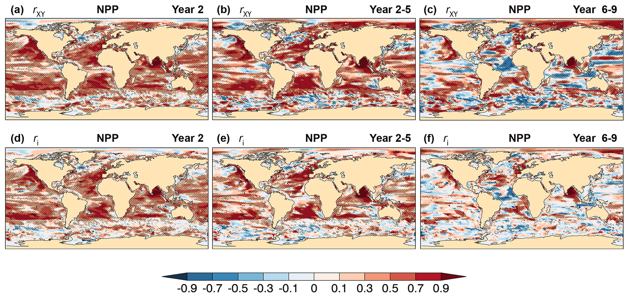
Figure 19Potential for skill of CanESM5 annual and multi-year mean of ocean NPP hindcasts. (a–c) Correlation skill rXY, Eq. (6), with the assimilation runs as verifying observations, and (d–f) contribution from initialization ri to correlation skill, Eq. (A17), for (a, d) Year 2, (b, e) Year 2–5, and (c, f) Year 6–9 hindcasts. The CanESM5 assimilation runs used as verifying observations provide the initial conditions of the hindcasts. Cross-hatched regions indicate values significantly different from zero at the 90 % confidence level.
Figure 19 shows the correlation skill rXY and the contribution from initialization ri of ocean NPP for Year 2, Year 2–5, and Year 6–9 hindcasts relative to the assimilation runs. For Year 2, there is significant correlation skill in most of the global ocean north of the Antarctic Circumpolar Current, except for scattered regions including WSPNA, the western North Pacific, and, to some degree, in the eastern equatorial regions of the Pacific and Atlantic oceans. These regions are characterized by relatively low prediction skill of upper-ocean heat content (Fig. 2a). High NPP correlation skill is found in most eastern ocean boundaries and coastal upwelling regions, and in broader sectors associated with boundary currents including the North Pacific and California currents, the Gulf Stream, North Atlantic and Canary currents, the Brazil and Benguela currents, the Agulhas Current, the East Australian Current, and in areas of the Arabian Sea and Bay of Bengal north of the Indian Monsoon Current. Part of this skill is attributed to initialization (Fig. 19d) with little or no impact from the simulated external forcing. Predictive skill tends to be larger in both magnitude and extent for Year 2–5 (Fig. 19b, e) and is much reduced for Year 6–9 (Fig. 19c, f), except for a few regions of relatively high skill including major eastern boundary upwelling systems (EBUSs; Chan, 2019). EBUSs comprise some of the ocean's most productive regions, supporting approximately one-fifth of the world's ocean wild fish harvests (Pauly and Christensen, 1995) and the habitats for multiple species of pelagic fish, migratory seabirds, and marine mammals (Block et al., 2011); thus, the potential for NPP skillful forecasts in these regions at relatively long lead times may have useful implications for fisheries and environmental managers. Preliminary comparisons against observation-based estimates over the Canary Current region (Fig. 21a), which, along with the California, Humboldt, and Benguela current systems, is one of the four major EBUSs (Gómez-Letona et al., 2017), show realistic interannual variations in the assimilation runs and Year 1 hindcasts. Ilyina et al. (2020) point out difficulties however in CanESM5 predictions of ocean CO2 uptake in an intercomparison of Earth system model results.
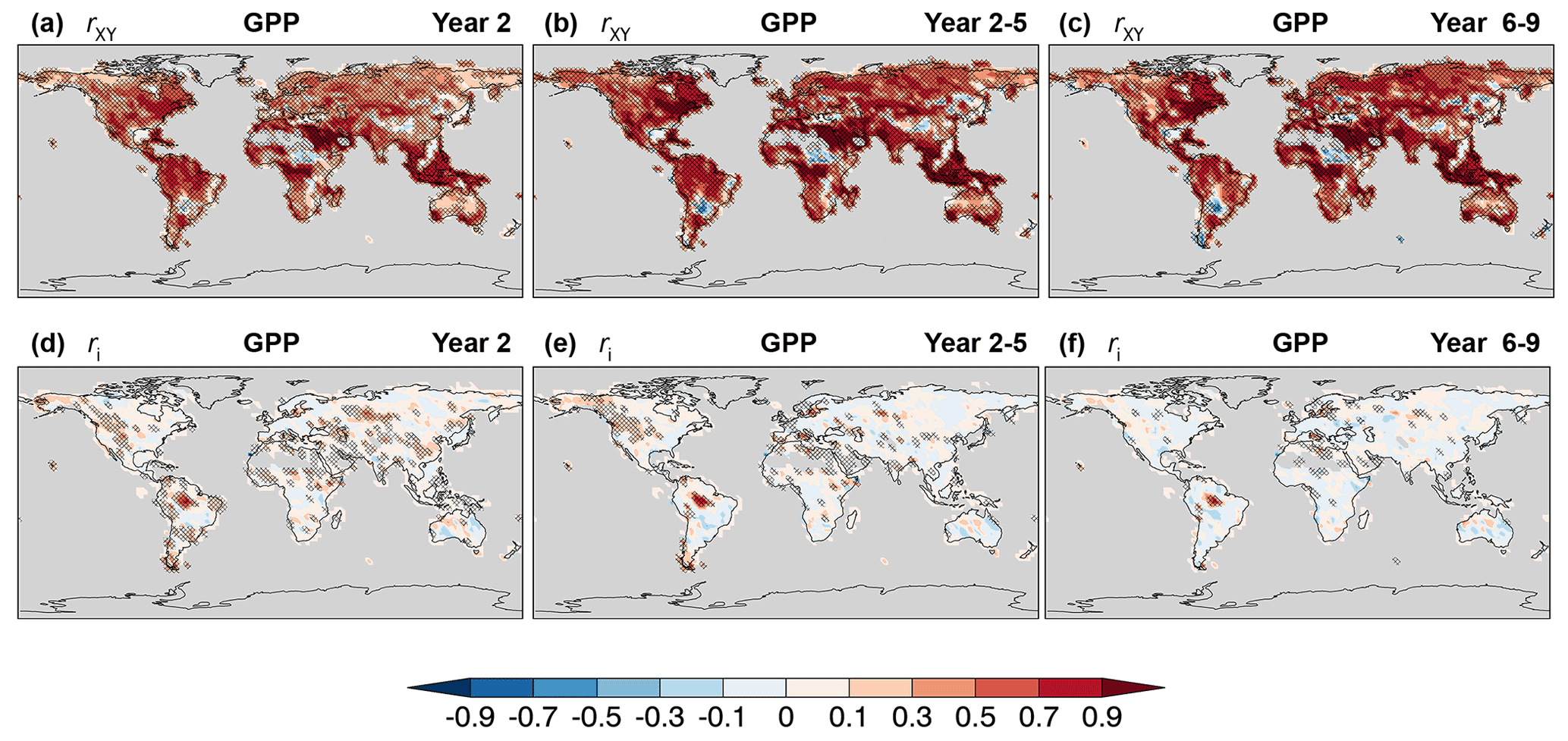
Figure 20As in Fig. 19 for GPP on land.
On land, significant GPP correlation skill of annual and multi-year hindcasts relative to the assimilation runs is found on all continents (Fig. 20a–c), although negative skill can be seen mainly in grassland and savanna regions of South America, Africa, and east Asia. Correlation skill is highest in the temperate zone of eastern North America, in southeast Asia and the Maritime Continent, in sectors of tropical South America and Africa, in southern Australia, and in north Africa, the Nile basin, and Arabian Peninsula. Except for the latter, these regions are characterized by moderate to high annual mean primary productivity (Fig. 1 of Field et al., 1998). Unlike ocean NPP, a large portion of GPP skill on land is derived from the simulated externally forced component, particularly from CO2 fertilization, with a moderate but significant contribution from initialization (Fig. 20d, e). The effects of initialization become negligible for longer forecast ranges, except for a small sector of the Amazon rainforest (Fig. 20f). Preliminary comparisons against observation-based products show realistic global mean GPP anomaly trends (not shown) and interannual variations for the assimilation runs and Year 1 hindcasts (Fig. 21b). This is consistent with multi-model comparisons (Ilyina et al., 2020) showing significant actual correlation skill of CO2 land uptake in linearly detrended CanESM5 assimilation runs and hindcasts for up to 2 years. Comparisons against observation-based data, however, are limited by the relatively short time span and uncertainty of the observations.
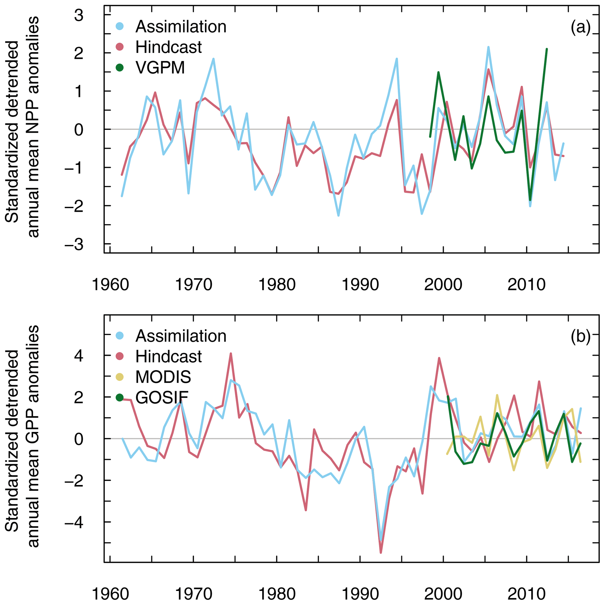
Figure 21(a) Ocean-integrated net primary productivity in the Canary Current region (25–34∘ N, 10–18∘ W), and (b) gross primary productivity on the global land, for the assimilation runs (blue) and Year 1 hindcasts (red). Observation-based estimates for (a) ocean, the Vertically Generalized Production Model (VGPM) (green), and (b) land, MODIS (yellow), and Orbiting Carbon Observatory-2 (OCO-2)-based solar-induced chlorophyll fluorescence (SIF) product (GOSIF) (green) are described in Appendix B. Anomalies relative to the base period (2000–2016) have been linearly detrended and standardized.
CanESM5 decadal hindcasts, which are CCCma's contribution to Component A of the DCPP component of CMIP6, have the ability to represent realistic interannual and multi-year variations of key physical climate fields and carbon cycle variables on decadal timescales. The hindcasts are 40-ensemble-member retrospective forecasts that are full-field initialized from realistic climate states at the end of every year during 1960 to the present and run for 10 years. Natural and anthropogenic external forcing associated with greenhouse gases and aerosols is specified, and a 40-member ensemble of historical uninitialized climate simulations with the same external forcing is also produced. The predictable component of the simulations is determined by the model's response to external forcing, whereas the forecasts have predictable components due to both the initialization of internal climate states and to the model's response to external forcing, which is generally different from that of simulations. The decomposition of the predictable component of the forecasts into initialized and uninitialized constituents, the latter derived from the projection of the forecasts responses to external forcing onto that of simulations, allowed the quantification of the impact of initialization on skill, and sheds new light on the value added by a forecasting system over that of climate simulations.
The upper-ocean heat content of CanESM5 is shown to be potentially predictable during the 10-year forecast range most notably in the extratropics, with potentially predictable variance in the eastern ocean boundaries for up to the 2- to 4-year range as a result of initialization. The hindcasts realize some of this potential predictability and have actual skill largely driven by external forcing, with significant contributions from initialization in the Pacific and Indian ocean basins. Sea surface temperature (SST) hindcasts are skillful for most of the global ocean mainly due to the strong warming response in the model, with a moderate impact from initialization to correlation skill beyond the first year of the hindcasts. Compared to heat content, SST is more directly affected by atmospheric conditions reducing the contribution of initialization to skill. Initialization also decreases MSE significantly relative to that of simulations in the northern subtropics and in the Indian Ocean due to a reduction of the simulated warming trend, which highlights the impact of initialization not only on the predictability of internal climate variations, but also on corrections of the simulated response to external forcing.
The western subpolar North Atlantic (WSPNA) and the Labrador Sea regions stand out for the negative skill of the upper-ocean heat content and the surface temperature, resulting in part from erroneous temperature and salinity trends in the reanalysis data used to initialize the forecasts. Winter SST variations of CanESM5 hindcasts in these regions have strong decadal variations that are out of phase with observations beyond the 1-year range. Also, strong cold biases and warming trends in the simulations contribute to the poor performance in these regions. The lack of skill in the WSPNA and the Labrador Sea merits further analysis as it may impact climate predictability elsewhere.
The strong warming response of CanESM5 drives the potential predictability of near-surface air temperature over land and is largely responsible for the hindcast correlation skill as examined in SB20. Initialization, however, reduces the strength of the model response to external forcing, leading to a lower hindcast MSE than that of the simulations and persistence at all forecast ranges considered, except for some tropical regions. The correlation skill of annual and multi-year mean precipitation is, perhaps surprisingly, very high in vast continental regions including Siberia, central southwestern Asia, northeastern Europe, the Americas, and the Sahel. The precipitation skill is mainly driven by external forcing, with a non-negligible impact from volcanic aerosols, although long-lived effects from initialization can be seen in regions such as northeastern Brazil and central southwestern Asia, which can be influenced by remote SST anomalies. Skill tends to be highest for multi-year averages, as potentially erroneous interannual variability is averaged out and the forced component becomes dominant.
Two additions to CCCma's contribution to the decadal prediction component of CMIP6 compared to CMIP5 are the increased ensemble size to 40 members from 10 members and the inclusion of carbon cycle variables in these experiments. There is growing evidence that large ensemble sizes are advantageous for decadal predictions, and this work is consistent with that view. Skillful CanESM5 precipitation hindcasts with a significant impact from initialization require large ensembles to confidently surpass the skill of uninitialized simulations, compared to 10 or fewer members. There is however a limit to the cost-effective increase of ensemble size needed to improve skill, which is determined by the ensemble forecast noise-to-predictable-variance ratio. Large ensembles are also used to show that CanESM5 decadal hindcasts underestimate the interannual and multi-year Sahelian summer rainfall signal, an important benchmark for the assessment of decadal predictions, as correlation skill is larger than potential correlation skill for sufficiently large ensembles despite the hindcasts having realistic total precipitation variance in this region. CanESM5 decadal hindcasts are skillful compared to assimilated values for predictions of net primary productivity in the ocean northward of the Antarctic Circumpolar Current for the 2- to 4-year range, with regions of long-lived skill encompassing the 10-year forecast range. A significant portion of this skill is attributed to initialization, particularly in major eastern boundary upwelling systems, where there is indication of actual skill as well, and in the Bay of Bengal. On land, gross primary productivity hindcasts have potential for skill at all ranges examined, mostly because of the CanESM5 response to the externally forced CO2 increase, with a moderate but significant short-lived impact from initialization. Preliminary comparisons of CanESM5 assimilation runs and Year 1 hindcasts with observation-based products have shown agreement in the global mean anomaly trend and interannual variations for the years of available data. A comprehensive assessment of actual skill remains, however, a challenge due the relatively short time span and uncertainty of the verifying observations.
A1 Associated variances
The variances associated with the ensembles of forecasts and simulations in Eq. (1), together with those of the ensemble mean of forecasts and simulations in Eq. (2), are
where we have used under the assumption of the yk's independence, and similarly for uk. The noise variances are estimated from Eqs. (A1)–(A4) as
whereas the predictable variance is estimated from Eqs. (A3)–(A6) as
The predictable and noise variances can be readily computed from the data by means of the total variance or , and the variance of the ensemble mean or . If we write explicitly the dependence of the anomaly forecast Yjk(τ) and ensemble mean Yj(τ) on the forecast range τ, ensemble member k=1…mY, and initial year j=1…n, then
and similarly for the simulations, where the overline indicates the average over the initial years.
A2 Correlation skill decomposition
Following SB20, the correlation skill of the ensemble mean forecast can be decomposed as
where and are the correlation skills of the uninitialized and initialized components Yu and Yi themselves, while ru and ri are the components contribution when scaled by the fractions of the variances involved. In terms of the noise-to-predictable-variance ratios of forecasts and simulation,
and available correlations and variances, these quantities can be computed explicitly as
where rYU denotes the correlation between the ensemble means of forecasts and simulations, and the step function θ=0 if rYU<0, else θ=1. The ratios γY and γU are estimated according to Eqs. (A12) and (A13) with the total variances and , Eq. (A9), and the ensemble mean variances and , Eq. (A10), for simulations and forecasts. For finite ensembles, and , and thus γU and γY, can be negative due to sampling errors. With Eqs. (A12)–(A13), the quantities in Eqs. (A16)–(A19) are readily computed from the data.
Table B1List of figures, CMIP6 variables, experiments, and verifying observation-based products employed in this paper. See Table B2 for the sources of the observation-based products. The entry “n/a” indicates “not applicable”.
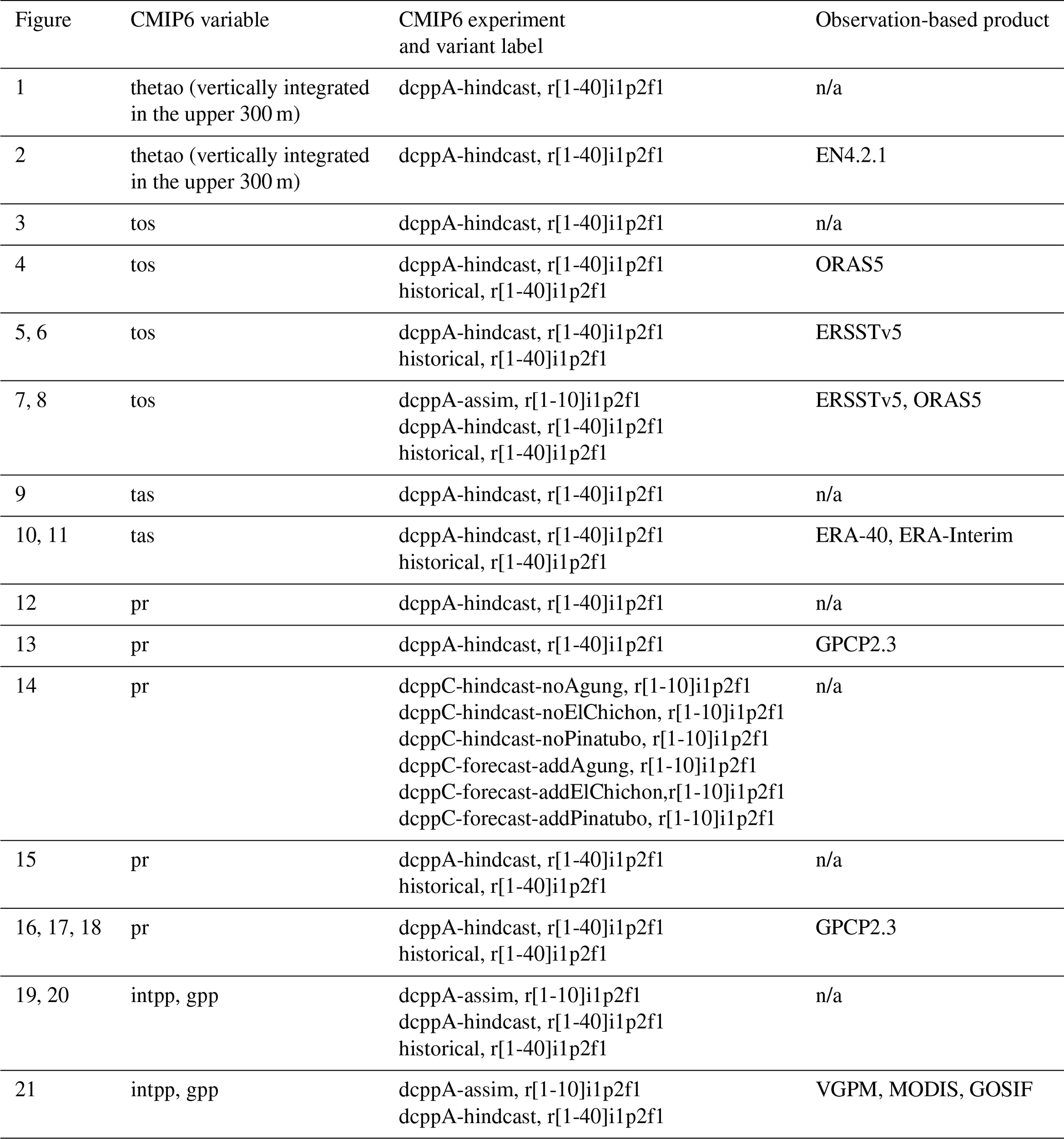
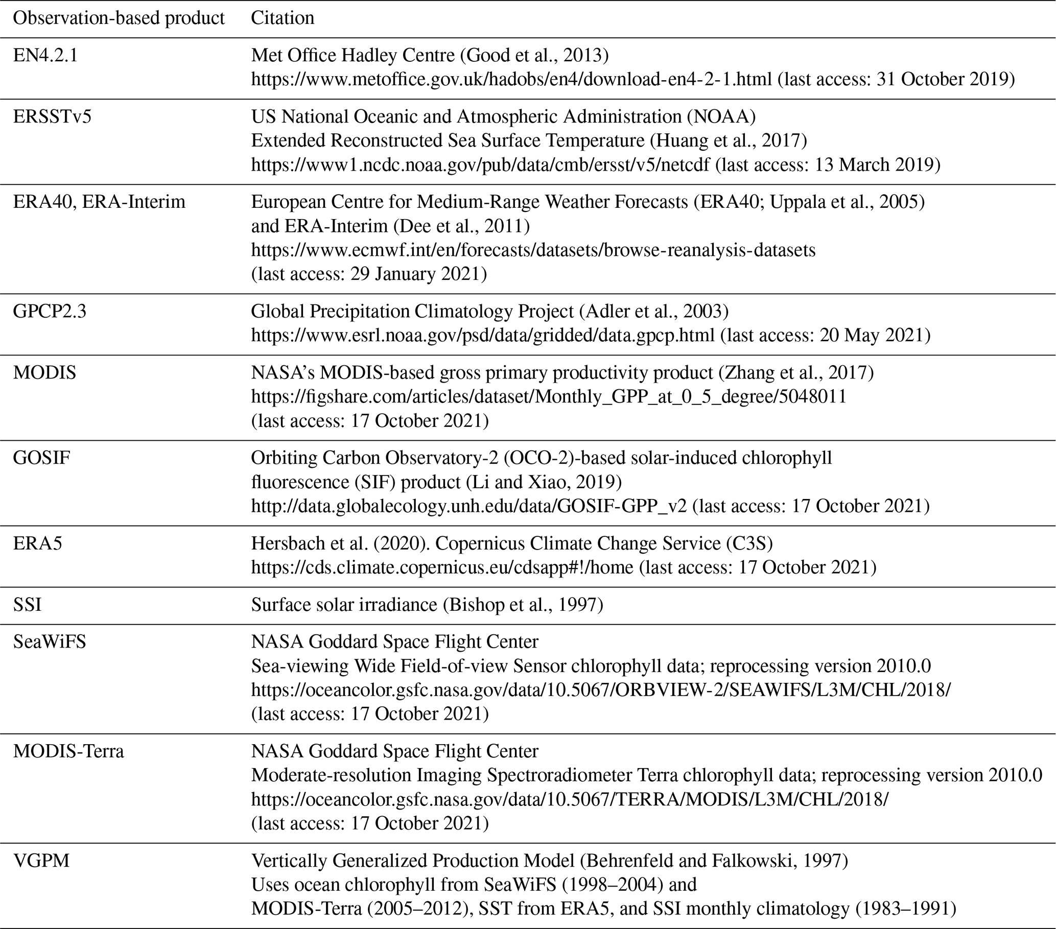
The CanESM5 source code is publicly available at https://gitlab.com/cccma/canesm (last access: 13 October 2021). The version of the code used to produce all the simulations described in this paper, which are submitted to CMIP6, is tagged as v5.0.3 with associated DOI: https://doi.org/10.5281/zenodo.3251114 (Swart et al., 2019a, b). The CanESM5 data for the decadal experiments (https://doi.org/10.22033/ESGF/CMIP6.3556, Sospedra-Alfonso et al., 2019a; https://doi.org/10.22033/ESGF/CMIP6.3557, Sospedra-Alfonso et al., 2019b; https://doi.org/10.22033/ESGF/CMIP6.3570, Sospedra-Alfonso et al., 2019c; https://doi.org/10.22033/ESGF/CMIP6.3571, Sospedra-Alfonso et al., 2019d; https://doi.org/10.22033/ESGF/CMIP6.3572, Sospedra-Alfonso et al., 2019e; https://doi.org/10.22033/ESGF/CMIP6.3573, Sospedra-Alfonso et al., 2019f; https://doi.org/10.22033/ESGF/CMIP6.3574, Sospedra-Alfonso et al., 2019g; https://doi.org/10.22033/ESGF/CMIP6.3575, Sospedra-Alfonso et al., 2019h) and historical simulations (https://doi.org/10.22033/ESGF/CMIP6.3610, Swart et al., 2019c) are publicly available from the Earth System Grid Federation (https://esgf-node.llnl.gov/search/cmip6/, last access: 13 October 2021). The observation-based products used here are freely available from the locations specified in Table B2 of Appendix B.
RSA initiated the study, helped to coordinate and performed model simulations, produced the analysis and figures, and wrote the paper. WJM led the experimental design and development of the CCCma contribution to DCPP and contributed with the analysis and interpretation of results. GJB was instrumental to the CCCma contribution to DCPP and contributed to the methodology, analysis, and interpretation of results. VVK and WSL set up and produced the bulk of model simulations. CS contributed with results, plotting, and assessment of GPP on land. JRC contributed with results and assessment of NPP in the ocean. All authors contributed with the manuscript and the final version of the paper.
The authors declare that they have no conflict of interest.
Publisher’s note: Copernicus Publications remains neutral with regard to jurisdictional claims in published maps and institutional affiliations.
We are thankful to the CCCma team at large for the development and production of the CanESM5 Earth system model. We are thankful also to Neil Swart and Michael Sigmund for their helpful comments on an earlier version of this paper. We acknowledge the various organizations listed in Table B2 for making the verification data used here freely available. This work is dedicated to the memory of our colleague and friend Fouad Majaess.
This paper was edited by Paul Halloran and reviewed by two anonymous referees.
Adler, R. F., Huffman, G., Chang, A., Ferraro, R., Xie, P., Janowiak, J., Rudolf, B., Schneider, U., Curtis, S., Bolvin, D., Gruber, A., Susskind, J., and Arkin, P.: The Version 2 Global Precipitation Climatology Project (GPCP) Monthly Precipitation Analysis (1979–Present), J. Hydrometeorol., 4, 1147–1167, 2003. a
Arora, V. K.: Simulating energy and carbon fluxes over winter wheat using coupled land surface and terrestrial ecosystem models, Agr. Forest Meteorol., 118, 21–47, 2003. a
Arora, V. K. and Boer, G. J.: A representation of variable root distribution in dynamic vegetation models, Earth Interact., 7, 1–19, 2003. a
Arora, V. K. and Boer, G. J.: A parameterization of leaf phenology for the terrestrial ecosystem component of climate models, Glob. Change Biol., 11, 39–59, 2005. a, b
Banzon, V., Smith, T. M., Chin, T. M., Liu, C., and Hankins, W.: A long-term record of blended satellite and in situ sea-surface temperature for climate monitoring, modeling and environmental studies, Earth Syst. Sci. Data, 8, 165–176, https://doi.org/10.5194/essd-8-165-2016, 2016. a
Barlow, M., Cullen, H., and Lyon, B. R.: Drought in Central and Southwest Asia: La Niña, the Warm Pool, and Indian Ocean Precipitation, J. Climate, 15, 697–700, 2002. a
Behrenfeld, M. J. and Falkowski, P. G.: Photosynthetic rates derived from satellite-based chlorophyll concentration, Limnol. Oceanogr., 42, 1–20, 1997. a
Biasutti, M.: Forced Sahel rainfall trends in the CMIP5 archive, J. Geophys. Res.-Atmos., 118, 1613–1623, 2013. a
Biasutti, M. and Giannini, A.: Robust Sahel drying in response to late 20th century forcings, Geophys. Res. Lett., 33, L11706, https://doi.org/10.1029/2006GL026067, 2006. a
Bishop, J. K. B., Rossow, W. B., and Dutton, E. G.: Surface solar irradiance from the International Satellite Cloud Climatology Project 1983–1991, J. Geophys. Res.-Atmos., 102, 6883–6910, 1997. a
Block, B. A., Jonsen, I. D., Jorgensen, S. J., Winship, A. J., Shaffer, S. A., Bograd, S. J., Hazen, E. L., Foley, D. G., Breed, G. A., Harrison, A.-L., Ganong, J. E., Swithenbank, A., Castleton, M., Dewar, H., Mate, B. R., Shillinger, G. L., Schaefer, K. M., Benson, S. R., Weise, M. J., Henry, R. W., and Costa, D. P.: Tracking apex marine predator movements in a dynamic ocean, Nature, 475, 86–90, 2011. a
Boer, G. J., Kharin, V. V., and Merryfield, W. J.: Decadal predictability and forecast skill, Clim. Dynam., 41, 1817–1833, 2013. a, b, c, d
Boer, G. J., Smith, D. M., Cassou, C., Doblas-Reyes, F., Danabasoglu, G., Kirtman, B., Kushnir, Y., Kimoto, M., Meehl, G. A., Msadek, R., Mueller, W. A., Taylor, K. E., Zwiers, F., Rixen, M., Ruprich-Robert, Y., and Eade, R.: The Decadal Climate Prediction Project (DCPP) contribution to CMIP6, Geosci. Model Dev., 9, 3751–3777, https://doi.org/10.5194/gmd-9-3751-2016, 2016. a, b, c, d, e, f, g
Boer, G. J., Kharin, V. V., and Merryfield, W. J.: Differences in potential and actual skill in a decadal prediction experiment, Clim. Dynam., 52, 6619–6631, 2019a. a, b, c
Boer, G. J., Merryfield, W. J., and Kharin, V. V.: Relationships between potential, attainable, and actual skill in a decadal prediction experiment, Clim. Dynam., 52, 4813–4831, 2019b. a, b, c, d
Bonfils, C. J. W., Santer, B. D., Fyfe, J. C., Marvel, K., Phillips, T. J., and Zimmerman, S. R. H.: Human influence on joint changes in temperature, rainfall and continental aridity, Nat. Clim. Change, 10, 726–731, https://doi.org/10.1038/s41558-020-0821-1, 2020. a
Bouillon, S., Maqueda, M. M., Legat, V., and Fichefet, T.: An elastic-viscous-plastic sea ice model formulated on Arakawa B and C grids, Ocean Model., 27, 174–184, 2009. a
Carrassi, A., Guemas, V., Doblas‐Reyes, F. J., Volpi, D., and Asif, M.: Sources of skill in near‐term climate prediction: generating initial conditions, Clim. Dynam., 47, 3693–3712, 2016. a
Chan, F.: Ocean deoxygenation: Everyone's problem – Causes, impacts, consequences and solutions, chap. Global and regional case studies of ocean deoxygenation/Evidence for ocean deoxygenation and its patterns: Eastern Boundary Upwelling Systems, IUCN, Gland, Switzerland, xxii+562 pp., 2019. a
Christian, J. R., Arora, V. K., Boer, G. J., Curry, C. L., Zahariev, K., Denman, K. L., Flato, G. M., Lee, W. G., Merryfield, W. J., Roulet, N. T., and Scinocca, J. F.: The global carbon cycle in the Canadian Earth system model (CanESM1): Preindustrial control simulation, J. Geophys. Res., 115, G03014, https://doi.org/10.1029/2008JG000920, 2010. a
Dee, P., Uppala, S. M., Simmons, A. J., Berrisford, P., Poli, P., Kobayashi, S., Andrae, S., Balmaseda, M., Balsamo, G., Bauer, P., Bechtold, P., Beljaars, A., van de Berg, L., Bidlot, J., Bormann, N., Delsol, C., Dragani, R., Fuentes, M., Geer, A. J., Haimberger, L., Healy, S. B., Hersbach, H., Hólm, E., Isaksen, L., Kȧllberg, P., Köhler, M., Matricardi, M., McNally, A., Monge-Sanz, B., Morcrette, J.-J., Park, B.-K., Peubey, C., de Rosnay, P., Tavolato, C., Thépaut, J.-N., and Vitart, F.: The ERA-Interim reanalysis: configuration and performance of the data assimilation system, Q. J. Roy. Meteor. Soc., 137, 553–597, 2011. a, b
Deser, C., Lehner, F., Rodgers, K. B., Ault, T., Delworth, T. L., DiNezio, P. N., Fiore, A., Frankignoul, C., Fyfe, J. C., Horton, D. E., Kay, J. E., Knutti, R., Lovenduski, N. S., Marotzke, J., McKinnon, K. A., Minobe, S., Randerson, J., Screen, J. A., Simpson, I. R., and Ting, M.: Insights from Earth system model initial-condition large ensembles and future prospects, Nat. Clim. Change, 10, 277–286, https://doi.org/10.1038/s41558-020-0731-2, 2020. a, b
Dirkson, A., Merryfield, W. J., and Monahan, A. H.: Impacts of sea ice thickness initialization on seasonal Arctic sea ice predictions, J. Climate, 30, 1001–1017, 2017. a
Doblas-Reyes, F. J., Balmaseda, M. A., Wisheimer, A., and Palmer, T. N.: Decadal climate prediction with the European Centre for Medium-Range Weather Forecasts coupled forecast system: Impact of ocean observations, J. Geophys. Res., 116, 1–13, 2011. a
Dong, B. and Sutton, R.: Dominant role of greenhouse-gas forcing in the recovery of Sahel rainfall, Nat. Clim. Change, 5, 757–760, https://doi.org/10.1038/nclimate2664, 2015. a
Dunstone, N. J., Smith, D. M., and Eade, R.: Multi‐year predictability of the tropical Atlantic atmosphere driven by the high latitude North Atlantic Ocean, Geophys. Res. Lett., 38, L14701, https://doi.org/10.1029/2011GL047949, 2011. a
Eade, R., Hamilton, E., Smith, D. M., Graham, R. J., and Scaife, A. A.: Forecasting the number of extreme daily events out to a decade ahead, J. Geophys. Res., 117, 1–12, 2012. a, b
Eade, R., Smith, D., Scaife, A., Wallace, E., Dunstone, N., Hermanson, L., and Robinson, N.: Do seasonal to decadal climate predictions underestimate the predictability of the real world?, Geophys. Res. Lett., 41, 5620–5628, 2014. a
Eyring, V., Bony, S., Meehl, G. A., Senior, C. A., Stevens, B., Stouffer, R. J., and Taylor, K. E.: Overview of the Coupled Model Intercomparison Project Phase 6 (CMIP6) experimental design and organization, Geosci. Model Dev., 9, 1937–1958, https://doi.org/10.5194/gmd-9-1937-2016, 2016. a
Fichefet, T. and Maqueda, M. M.: Sensitivity of a global sea ice model to the treatment of ice thermodynamics and dynamics, J. Geophys. Res., 102, 12609–12646, 1997. a
Field, C. B., Behrenfeld, M. J., Randerson, J. T., and Falkowski, P.: Primary Production of the Biosphere: Integrating Terrestrial and Oceanic Components, Science, 281, 237–240, 1998. a, b
Gaetani, M. and Mohino, E.: Decadal Prediction of the Sahelian Precipitation in CMIP5 Simulations, J. Climate, 26, 7708–7719, 2013. a, b, c
Garcia-Serrano, J., Doblas-Reyes, F. J., Haarsma, R. J., and Polo, I.: Decadal prediction of the dominant West African monsoon rainfall modes, J. Geophys. Res., 118, 5260–5279, 2013. a
García-Serrano, J., Guemas, V., and Doblas-Reyes, F. J.: Added-value from initialization in predictions of Atlantic multi-decadal variability, Clim. Dynam., 44, 2539–2555, 2015. a
Goddard, G. J., Kumar, A., Solomon, A., Smith, D., Boer, G., González, P., Kharin, V., Merryfield, W., Deser, C., Mason, S. J., Kirtman, B. P., Msadek, R., Sutton, R., Hawkins, E., Fricker, T., Hegerl, G., Ferro, C. A. T., Stephenson, D. B., Meel, G. A., Stockdale, T., Burgman, R., Greene, A. M., Kushnir, Y., Newman, M., Carton, J., Fukumori, I., and Delworth, T.: A verification framework for interannual-to-decadal predictions experiments, Clim. Dynam., 40, 245–272, 2013. a, b, c, d
Gómez-Letona, M., Ramos, A. G., Coca, J., and Arístegui, J.: Trends in Primary Production in the Canary Current Upwelling System – A Regional Perspective Comparing Remote Sensing Models, Frontiers Marine Science, 4, 370, https://doi.org/10.3389/fmars.2017.00370, 2017. a
Good, S. A., Martin, M. J., and Rayner, N. A.: EN4: quality controlled ocean temperature and salinity profiles and monthly objective analyses with uncertainty estimates, J. Geophys. Res., 118, 6704–6716, 2013. a
Gough, C. M.: Terrestrial Primary Production: Fuel for Life, Nature Education Knowledge, 3, available at: https://www.nature.com/scitable/knowledge/library/terrestrial-primary-production-fuel-for-life-17567411/ (last access: 17 October 2021), 2011. a
Haarsma, R. J., Selten, F. M., Weber, S. L., and Kliphuis, M.: Sahel rainfall variability and response to greenhouse warming, Geophys. Res. Letters, 32, L17702, https://doi.org/10.1029/2005GL023232, 2005. a
Haywood, J. M., Jones, A., Bellouin, N., and Stephenson, D.: Asymmetric forcing from stratospheric aerosols impacts Sahelian rainfall, Nat. Clim. Change, 3, 660–665, https://doi.org/10.1038/NCLIMATE1857, 2013. a
Hersbach, H., Bell, B., Berrisford, P., Hirahara, S., Horanyi, A., Munoz-Sabater, J., Nicolas, J., Peubey, C., Radu, R., Schepers, D., Simmons, A., Soci, C., Abdalla, S., Abellan, X., Balsamo, G., Bechtold, P., Biavati, G., Bidlot, J., Bonavita, M., De Chiara, G., Dahlgren, P., Dee, D., Diamantakis, M., Dragani, R., Flemming, J., Forbes, R., Fuentes, M., Geer, A., Haimberger, L., Healy, S., Hogan, R., J., Holm, E., Janiskova, M., Keeley, S., Laloyaux, P., Lopez, P., Lupu, C., Radnoti, G., de Rosnay, P., Rozum, I., Vamborg, F., Villaume, S., and Thepaut, J.-N.: The ERA5 global reanalysis, Q. J. Roy. Meteor. Soc., 146, 1999–2049, 2020. a
Hua, W., Dai, A., Zhou, L., Qin, M., and Chen, H.: An externally forced decadal rainfall seesaw pattern over the Sahel and southeast Amazon, Geophys. Res. Lett., 46, 923–932, https://doi.org/10.1029/2018GL081406, 2019. a
Huang, B., Thorne, P. W., Banzon, V. F., Boyer, T., Chepurin, G., Lawrimore, J. H., Menne, M. J., Smith, T. M., Vose, R. S., and Zhang, H.-M.: Extended Reconstructed Sea Surface Temperature version 5 (ERSSTv5), Upgrades, validations, and intercomparisons, J. Climate, 30, 8179–8205, 2017. a
Ilyina, T., Li, H., , Spring, A., Müller, W. A., Bopp, L., Chikamoto, M. O., Danabasoglu, G., Dobrynin, M., Dunne, J., Fransner, F., Friedlingstein, P., Lee, W., Lovenduski, N. S., Merryfield, W., Mignot, J., Park, J., Séférian, R., Sospedra-Alfonso, R., Watanabe, M., and Yeager, S.: Predictable variations of the carbon sinks and atmospheric CO2 growth in a multi-model framework, Geophys. Res. Lett., 48, e2020GL090695, https://doi.org/10.1029/2020GL090695, 2020. a, b
Jackson, L. C., Dubois, C., Forget, G., Haines, K., Harrison, M., Iovino, D., Kohl, A., Mignac, D., Masina, S., Peterson, K. A., Piecuch, C. G., Roberts, C. D., Robson, J., Storto, A., Toyoda, T., Valdivieso, M., Wilson, C., Wang, Y., , and Zuo, H.: The mean state and variability of the North Atlantic circulation: A perspective from Ocean Reanalyses, J. Geophys. Res.-Oceans, 124, 9141–9170, 2019. a, b
Johnson, S. J., Stockdale, T. N., Ferranti, L., Balmaseda, M. A., Molteni, F., Magnusson, L., Tietsche, S., Decremer, D., Weisheimer, A., Balsamo, G., Keeley, S. P. E., Mogensen, K., Zuo, H., and Monge-Sanz, B. M.: SEAS5: the new ECMWF seasonal forecast system, Geosci. Model Dev., 12, 1087–1117, https://doi.org/10.5194/gmd-12-1087-2019, 2019. a
Knight, J. R., Folland, C. K., and Scaife, A. A.: Climate impacts of the Atlantic Multidecadal Oscillation, Geophys. Res. Lett., 33, L17706, https://doi.org/10.1029/2006GL026242, 2006. a
Levitus, S., Antonov, J. I., Boyer, T. P., Garcia, H. E., and Locarnini, R. A.: EOF analysis of upper ocean heat content, 1956–2003, Geophys. Res. Lett., 32, 1–4, 2005. a
Li, X. and Xiao, J.: Mapping Photosynthesis Solely from Solar-Induced Chlorophyll Fluorescence: A Global, Fine-Resolution Dataset of Gross Primary Production Derived from OCO-2, Remote Sens., 11, 2563, https://doi.org/10.3390/rs11212563, 2019. a
Lindzen, R. S. and Nigam, S.: On the role of sea surface temperature gradients in forcing low level winds and convergence in the tropics, J. Atmos. Sci., 44, 2418–2436, 1987. a
Madec, G. and the NEMO team: NEMO ocean engine, version 3.4, Note du Pole de Modélisation 27, Institut Pierre-Simon Laplace, France, 367 pp., 2012. a
Martin, E. R. and Thorncroft, C. D.: Sahel rainfall in multimodel CMIP5 decadal hindcasts, Geophys. Res. Lett., 41, 2169–2175, 2014a. a, b, c
Martin, E. R. and Thorncroft, C. D.: The impact of the AMO on the West African monsoon annual cycle, Q. J. Roy. Meteor. Soc., 140, 31–46, 2014b. a, b
McKinnon, K. A., Rhines, A., Tingley, M. P., and Huybers, P.: Long-lead predictions of eastern United States hot days from Pacific sea surface temperatures, Nat. Geosci., 9, 389–394, 2016. a
Meehl, G. A., Goddard, L., Murphy, J., Stouffer, R. J., Boer, G., Danabasoglu, G., Dixon, K., Giorgetta, M. A., Greene, A. M., Hawkins, E., Hegerl, G., Karoly, D., Keenlyside, N., Kimoto, M., Kirtman, B., Navarra, A., Pulwarty, R., Smith, D., Stammer, D., and Stockdale, T.: Decadal prediction: Can it be skillful, B. Am. Metheorol. Soc., 90, 1467–1485, 2009. a, b
Meehl, G. A., Goddard, L., Boer, G., Burgman, R., Branstator, G., Cassou, C., Corti, S., Danabasoglu, G., Doblas-Reyes, F., Hawkins, E., Karspeck, A., Kimoto, M., Kumar, A., Matei, D., Mignot, J., Msadek, R., Navarra, A., Pohlmann, H., Rienecker, M., Rosati, T., Schneider, E., Smith, D., Sutton, R., Teng, H., G. J. van Oldenborgh, G. V., and Yeager, S.: Decadal climate prediction: An update from the trenches, B. Am. Metheorol. Soc., 95, 243–267, 2014. a
Meehl, G. A., Senior, C. A., Eyring, V., Flato, G., Lamarque, J.-F., Stouffer, R. J., Taylor, K. E., and Schlund, M.: Context for interpreting equilibrium climate sensitivity and transient climate response from the CMIP6 Earth system models, Sci. Adv., 6, eaba1981, https://doi.org/10.1126/sciadv.aba1981, 2020. a
Melton, J. R. and Arora, V. K.: Competition between plant functional types in the Canadian Terrestrial Ecosystem Model (CTEM) v. 2.0, Geosci. Model Dev., 9, 323–361, https://doi.org/10.5194/gmd-9-323-2016, 2016. a
Merryfield, W. J., Lee, W.-S., Boer, G. J., Kharin, V. V., Scinocca, J. F., Flato, G. M., Ajayamohan, R. S., and Fyfe, J. C.: The Canadian Seasonal to Interannual Prediction System. Part I: Models and Initialization, Mon. Weather Rev., 141, 2910–2945, 2013. a, b
Merryfield, W. J., Baehr, J., Batte, L., Becker, E. J., Butler, A. H., Coelho, C. A. S., Danabasoglu, G., Dirmeyer, P. A., Doblas-Reyes, F. J., Domeisen, D. I. V., Ferranti, L., Ilynia, T., Kumar, A., Muller, W. A., Rixen, M., Robertson, A. W., Smith, D. M., Takaya, Y., Tuma, M., Vitart, F., White, C. J., Alvarez, M. S., Ardilouze, C., Attard, H., Baggett, C., Balmaseda, M. A., Beraki, A. F., Bhattacharjee, P. S., Bilbao, R., de Andrade, F. M., DeFlorio, M. J., Diaz, L. B., Ehsan, M. A., Fragkoulidis, G., Grainger, S., Green, B. W., Hell, M. C., Infanti, J. M., Isensee, K., Kataoka, T., Kirtman, B. P., Klingaman, N. P., Lee, J.-Y., Mayer, K., McKay, R., Mecking, J. V., Miller, D. E., Neddermann, N., Ng, C. H. J., Osso, A., Pankatz, K., , Peatman, S., Pegion, K., Perlwitz, J., Recalde-Coronel, G. C., Reintges, A., Renk, C., Solaraju-Murali, B., Spring, A., Stan, C., Sun, Y. Q., Tozer, C. R., Vigaud, N., Woolnough, S., and Yeager, S.: Current and emerging developments in subseasonal to decadal prediction, B. Am. Metheorol. Soc., 101, E869–E896, https://doi.org/10.1175/BAMS-D-19-0037.1, 2020. a
Mohino, E., Rodriguez-Fonseca, B., Losada, T., Gervois, S., Janicot, S., Bader, J., Ruti, P., and Chauvin, F.: Changes in the interannual SST-forced signals on West African rainfall. AGCM intercomparison, Clim. Dynam., 37, 1707–1725, 2011a. a
Mohino, E., Rodriguez-Fonseca, B., Mechoso, C. R., Gervois, S., Ruti, P., and Chauvin, F.: Impacts of the Tropical Pacific/Indian Oceans on the Seasonal Cycle of the West African Monsoon, J. Climate, 24, 3878–3891, 2011b. a
Monerie, P.-A., Robson, J., Dong, B., and Dunstone, N.: A role of the Atlantic Ocean in predicting summer surface air temperature over North East Asia, Clim. Dynam., 51, 473–491, 2018. a
Myhre, G., Forster, P. M., Samset, B. H., Hodnebrog, O., Sillmann, J., Aalbergsjo, S. G., Andrews, T., Boucher, O., Faluvegi, G., Flaschner, D., Iversen, T., Kasoar, M., Kharin, V. V., Kirkevag, A., Lamarque, J.-F., Olivie, D., Richardson, T. B., Shindell, D., Shine, K. P., Stjern, C. W., Takemura, T., Voulgarakis, A., and Zwiers, F.: PDRMIP: A Precipitation Driver and Response Model Intercomparison Project – Protocol and Preliminary Results, B. Am. Metheorol. Soc., 98, 1185–1198, 2017. a
Nobre, P., Marengo, J. A., Cavalcanti, I. F. A., Obregon, G., Barros, V., and Camilloni, I.: Seasonal-to-Decadal Predictability and Prediction of South American Climate, J. Climate, 19, 5988–6004, 2005. a
Orr, J. C., Najjar, R. G., Aumont, O., Bopp, L., Bullister, J. L., Danabasoglu, G., Doney, S. C., Dunne, J. P., Dutay, J.-C., Graven, H., Griffies, S. M., John, J. G., Joos, F., Levin, I., Lindsay, K., Matear, R. J., McKinley, G. A., Mouchet, A., Oschlies, A., Romanou, A., Schlitzer, R., Tagliabue, A., Tanhua, T., and Yool, A.: Biogeochemical protocols and diagnostics for the CMIP6 Ocean Model Intercomparison Project (OMIP), Geosci. Model Dev., 10, 2169–2199, https://doi.org/10.5194/gmd-10-2169-2017, 2017. a
Pauly, D. and Christensen, V.: Primary production required to sustain global fisheries, Nature, 374, 255–257, 1995. a
Rowell, D. P.: The impact of Mediterranean SSTs on the Sahelian rainfall season, J. Climate, 16, 849–862, 2003. a
Rowell, D. P., Folland, C. K., Maskell, K., and Ward, M. N.: Variability of summer rainfall over tropical north Africa (1906–92) Observations and modelling, Q. J. Roy. Meteor. Soc., 121, 669–704, 1995. a
Ruprich-Robert, Y., Msadek, R., Castruccio, F., Yeager, S., Delworth, T., and Danabasoglu, G.: Assessing the Climate Impacts of the Observed Atlantic Multidecadal Variability Using the GFDL CM2.1 and NCAR CESM1 Global Coupled Models, J. Climate, 30, 2785–2810, 2017a. a
Ruprich-Robert, Y., Msadek, R., Castruccio, F., Yeager, S., Delworth, T., and Danabasoglu, G.: Assessing the climate impacts of the observed Atlantic multidecadal variability using the GFDL CM2.1 and NCAR CESM1 Global Coupled Models, J. Climate, 30, 2785–2809, 2017b. a
Ruprich-Robert, Y., Delworth, T., Msadek, R., Castruccio, F., Yeager, S., and Danabasoglu, G.: Impacts of the Atlantic multidecadal variability on North American summer climate and heat waves, J. Climate, 31, 3679–3700, 2018. a
Scaife, A. A. and Smith, S.: A signal-to-noise paradox in climate science, npj Climate and Atmospheric Science, 1, 28, https://doi.org/10.1038/s41612-018-0038-4, 2018. a, b, c, d
Schiemann, R., Luthi, D., Vidale, P. L., and Schar, C.: The precipitation climate of Central Asia – intercomparison of boservational and numerical data sources in a remote semiarid region, Int. J. Climatol., 28, 295–314, 2008. a
Sheen, K. L., Smith, D. M., Dunstone, N. J., Eade, R., Rowell, D. P., and Vellinga, M.: Skilful prediction of Sahel summer rainfall on inter-annual and multi-year timescales, Nat. Commun., 8, 1–12, 2017. a, b, c, d, e
Sienz, F., Müller, W. A., and Pohlmann, H.: Ensemble size impact on the decadal predictive skill assessment, Meteorol. Z., 25, 645–655, https://doi.org/10.1127/metz/2016/0670, 2016. a
Sigman, D. M. and Hain, M. P.: The Biological Productivity of the Ocean, Nature Education, 3, available at: https://www.nature.com/scitable/knowledge/library/the-biological-productivity-of-the-ocean-70631104/ (last access: 17 October 2021), 2012. a
Smith, D. M., Cusack, S., Colman, A. W., Folland, C. K., Harris, G. R., and Murphy, J. M.: Improved surface temperature prediction for the coming decade from a Global Climate Model, Science, 317, 796–799, 2007. a, b
Smith, D. M., Eade, R., Dunstone, N. J., Fereday, D., Murphy, J. M., Pohlmann, H., and Scaife, A. A.: Skilful climate model predictions of multi-year north Atlantic hurricane frequency, Nat. Geosci., 3, 846–849, 2010. a
Smith, D. M., Scaife, A. A., and Kirtman, B. P.: What is the current state of scientific knowledge with regard to seasonal and decadal forecasting?, Envrion. Res. Lett., 7, 1–11, 2012. a, b
Smith, D. M., Eade, R., Scaife, A. A., Caron, L.-P., Danabasoglu, G., DelSole, T. M., Delworth, T., Doblas-Reyes, F. J., Dunstone, N. J., Hermanson, L., Kharin, V., Kimoto, M., Merryfield, W. J., Mochizuki, T., Müller, W. A., Pohlmann, H., Yeager, S., and Yang, X.: Robust skill of decadal climate predictions, npj Climate And Atmospheric Science, 13, 1–10, 2019. a, b, c, d
Smith, D. M., Scaife, A. A., Eade, R., Athanasiadis, P., Bellucci, A., Bethke, I., Bilbao, R., Borchert, L. F., Caron, L.-P., Counillon, F., Danabasoglu, G., Delworth, T., Doblas-Reyes, F. J., Dunstone, N. J., Estella-Perez, V., Flavoni, S., Hermanson, L., Keenlyside, N., Kharin, V., Kimoto, M., Merryfield, W. J., Mignot, J., Mochizuki, T., Modali, K., Monerie, P.-A., Muller, W. A., Nicoli, D., Ortega, P., Pankatz, K., Pohlmann, H., Robson, J., Ruggieri, P., Sospedra-Alfonso, R., Swingedouw, D., Wang, Y., Wild, S., Yeager, S., Yang, X., and Zhang, L.: North Atlantic climate far more predictable than models imply, Nature, 583, 796–800, https://doi.org/10.1038/s41586-020-2525-0, 2020. a, b, c, d
Smith, T. M., Reynolds, R., Peterson, T., and Lawrimore, J.: Improvements NOAAs Historical Merged Land-Ocean Temp Analysis, J. Climate, 21, 2283–2296, 2008. a
Sospedra-Alfonso, R. and Boer, G. J.: Assessing the impact of initialization on decadal prediction skill, Geophys. Res. Lett., 47, e2019GL086361, https://doi.org/10.1029/2019GL086361, 2020. a, b, c
Sospedra-Alfonso, R., Lee, W., Merryfield, W. J., Swart, N. C., Cole, J. N. S., Kharin, V. V., Lazare, M., Scinocca, J. F., Gillett, N. P., Anstey, J., Arora, V., Christian, J. R., Jiao, Y., Lee, W. G., Majaess, F., Saenko, O. A., Seiler, C., Seinen, C., Shao, A., Solheim, L., von Salzen, K., Yang, D., Winter, B., and Sigmond, M.: CCCma CanESM5 model output prepared for CMIP6 DCPP dcppA-assim, Earth System Grid Federation [data set], https://doi.org/10.22033/ESGF/CMIP6.3556, 2019a. a
Sospedra-Alfonso, R., Lee, W., Merryfield, W. J., Swart, N. C., Cole, J. N. S., Kharin, V. V., Lazare, M., Scinocca, J. F., Gillett, N. P., Anstey, J., Arora, V., Christian, J. R., Jiao, Y., Lee, W. G., Majaess, F., Saenko, O. A., Seiler, C., Seinen, C., Shao, A., Solheim, L., von Salzen, K., Yang, D., Winter, B., and Sigmond, M.: CCCma CanESM5 model output prepared for CMIP6 DCPP dcppA-hindcast, Earth System Grid Federation [data set], https://doi.org/10.22033/ESGF/CMIP6.3557, 2019b. a
Sospedra-Alfonso, R., Lee, W., Merryfield, W. J., Swart, N. C., Cole, J. N. S., Kharin, V. V., Lazare, M., Scinocca, J. F., Gillett, N. P., Anstey, J., Arora, V., Christian, J. R., Jiao, Y., Lee, W. G., Majaess, F., Saenko, O. A., Seiler, C., Seinen, C., Shao, A., Solheim, L., von Salzen, K., Yang, D., Winter, B., and Sigmond, M.: CCCma CanESM5 model output prepared for CMIP6 DCPP dcppC-forecast-addAgung, Earth System Grid Federation [data set], https://doi.org/10.22033/ESGF/CMIP6.3570, 2019c. a
Sospedra-Alfonso, R., Lee, W., Merryfield, W. J., Swart, N. C., Cole, J. N. S., Kharin, V. V., Lazare, M., Scinocca, J. F., Gillett, N. P., Anstey, J., Arora, V., Christian, J. R., Jiao, Y., Lee, W. G., Majaess, F., Saenko, O. A., Seiler, C., Seinen, C., Shao, A., Solheim, L., von Salzen, K., Yang, D., Winter, B., and Sigmond, M.: CCCma CanESM5 model output prepared for CMIP6 DCPP dcppC-forecast-addElChichon, Earth System Grid Federation [data set], https://doi.org/10.22033/ESGF/CMIP6.3571, 2019d. a
Sospedra-Alfonso, R., Lee, W., Merryfield, W. J., Swart, N. C., Cole, J. N. S., Kharin, V. V., Lazare, M., Scinocca, J. F., Gillett, N. P., Anstey, J., Arora, V., Christian, J. R., Jiao, Y., Lee, W. G., Majaess, F., Saenko, O. A., Seiler, C., Seinen, C., Shao, A., Solheim, L., von Salzen, K., Yang, D., Winter, B., and Sigmond, M.: CCCma CanESM5 model output prepared for CMIP6 DCPP dcppC-forecast-addPinatubo, Earth System Grid Federation [data set], https://doi.org/10.22033/ESGF/CMIP6.3572, 2019e. a
Sospedra-Alfonso, R., Lee, W., Merryfield, W. J., Swart, N. C., Cole, J. N. S., Kharin, V. V., Lazare, M., Scinocca, J. F., Gillett, N. P., Anstey, J., Arora, V., Christian, J. R., Jiao, Y., Lee, W. G., Majaess, F., Saenko, O. A., Seiler, C., Seinen, C., Shao, A., Solheim, L., von Salzen, K., Yang, D., Winter, B., and Sigmond, M.: CCCma CanESM5 model output prepared for CMIP6 DCPP dcppC-forecast-noAgung, Earth System Grid Federation [data set], https://doi.org/10.22033/ESGF/CMIP6.3573, 2019f. a
Sospedra-Alfonso, R., Lee, W., Merryfield, W. J., Swart, N. C., Cole, J. N. S., Kharin, V. V., Lazare, M., Scinocca, J. F., Gillett, N. P., Anstey, J., Arora, V., Christian, J. R., Jiao, Y., Lee, W. G., Majaess, F., Saenko, O. A., Seiler, C., Seinen, C., Shao, A., Solheim, L., von Salzen, K., Yang, D., Winter, B., and Sigmond, M.: CCCma CanESM5 model output prepared for CMIP6 DCPP dcppC-forecast-noElChichon, Earth System Grid Federation [data set], https://doi.org/10.22033/ESGF/CMIP6.3574, 2019g. a
Sospedra-Alfonso, R., Lee, W., Merryfield, W. J., Swart, N. C., Cole, J. N. S., Kharin, V. V., Lazare, M., Scinocca, J. F., Gillett, N. P., Anstey, J., Arora, V., Christian, J. R., Jiao, Y., Lee, W. G., Majaess, F., Saenko, O. A., Seiler, C., Seinen, C., Shao, A., Solheim, L., von Salzen, K., Yang, D., Winter, B., and Sigmond, M.: CCCma CanESM5 model output prepared for CMIP6 DCPP dcppC-forecast-noPinatubo, Earth System Grid Federation [data set], https://doi.org/10.22033/ESGF/CMIP6.3575, 2019h. a
Strommen, K. and Palmer, T. N.: Signal and noise in regime systems: A hypothesis on the predictaility of the North Atlantic Oscillation, Q. J. Roy. Meteor. Soc., 145, 147–163, 2019. a
Sutton, R. T. and Dong, B.: Atlantic Ocean influence on a shift in European climate in the 1990s, Nat. Geosci., 5, 788–792, 2012. a
Swart, N. C., Cole, J., Kharin, S., Lazare, M. S. J., Gillett, N., Anstey, J., Arora, V., Christian, J., Hanna, S., Jiao, Y., Lee, W., Majaess, F., Saenko, O., Seiler, C., Seinen, C., Shao, A., Solheim, L., von Salzen, K., Yang, D., and Winter, B.: The Canadian Earth System Model (CanESM), v5.0.3., Zenodo [code], https://doi.org/10.5281/zenodo.3251114, 2019a. a
Swart, N. C., Cole, J. N. S., Kharin, V. V., Lazare, M., Scinocca, J. F., Gillett, N. P., Anstey, J., Arora, V., Christian, J. R., Hanna, S., Jiao, Y., Lee, W. G., Majaess, F., Saenko, O. A., Seiler, C., Seinen, C., Shao, A., Sigmond, M., Solheim, L., von Salzen, K., Yang, D., and Winter, B.: The Canadian Earth System Model version 5 (CanESM5.0.3), Geosci. Model Dev., 12, 4823–4873, https://doi.org/10.5194/gmd-12-4823-2019, 2019b. a, b
Swart, N. C., Cole, J. N. S., Kharin, V. V., Lazare, M., Scinocca, J. F., Gillett, N. P., Anstey, J., Arora, V., Christian, J. R., Jiao, Y., Lee, W. G., Majaess, F., Saenko, O. A., Seiler, C., Seinen, C., Shao, A., Solheim, L., von Salzen, K., Yang, D., Winter, B., and Sigmond, M.: CCCma CanESM5 model output prepared for CMIP6 CMIP historical, Earth System Grid Federation [data set], https://doi.org/10.22033/ESGF/CMIP6.3610, 2019c. a
Taguchi, B., Schneider, N., Nonaka, M., and Sasaki, H.: Decadal Variability of Upper-Ocean Heat Content Associated with Meridional Shifts of Western Boundary Current Extensions in the North Pacific, J. Climate, 30, 6247–6264, 2017. a
Taylor, K. E., Stouffer, R. J., and Meehl, G. A.: An overview of CMIP5 and the experiment design, B. Am. Meteorol. Soc., 92, 485–498, 2012. a
Tietsche, S., Balmaseda, M., Zuo, H., Roberts, C., Mayer, M., and Ferranti, L.: The importance of North Atlantic Ocean transports for seasonal forecasts, Clim. Dynam., 55, 1995–2011, https://doi.org/10.1007/s00382-020-05364-6, 2020. a, b
Ting, M., Kushnir, Y., Seager, R., and Li, C.: Forced and Internal Twentieth-Century SST Trends in the North Atlantic, J. Climate, 22, 1469–1481, 2009. a
Tippett, M. K., Barlow, M., and Lyon, B.: Statistical correction of Central Southwest Asian winter precipitation simulations, Int. J. Climatol., 23, 1421–1433, 2003. a, b
Titchner, H. A. and Rayner, N. A.: The Met Office Hadley Centre sea ice and sea surface temperature data set, version 2: 1. Sea ice concentrations, J. Geophys. Res.-Atmos., 119, 2864–2889, 2014. a
Tivy, A., Howell, S. E. L., Alt, B., McCourt, S., Chagnon, R., Crocker, G., Carrieres, T., and Yackel, J. J.: Trends and variability in summer sea ice cover in the Canadian Arctic based on the Canadian Ice Service Digital Archive, 1960–2008 and 1968–2008, J. Geophys. Res., 116, C03007, https://doi.org/10.1029/2009JC005855, 2011. a
Uppala, S. M., KAllberg, P. W., Simmons, A. J., Andrae, U., Bechtold, V. D. C., Fiorino, M., Gibson, J. K., Haseler, J., Hernandez, A., Kelly, G. A., Li, X., Onogi, K., Saarinen, S., Sokka, N., Allan, R. P., Andersson, E., Arpe, K., Balmaseda, M. A., Beljaars, A. C. M., Berg, L. V. D., Bidlot, J., Bormann, N., Caires, S., Chevallier, F., Dethof, A., Dragosavac, M., Fisher, M., Fuentes, M., Hagemann, S., Hólm, E., Hoskins, B. J., Isaksen, L., Janssen, P. A. E. M., Jenne, R., amd J.‐F. Mahfouf, A. P. M., Morcrette, J., Rayner, N. A., Saunders, R. W., Simon, P., Sterl, A., Trenberth, K. E., Untch, A., Vasiljevic, D., Viterbo, P., and Woollen, J.: The ERA-40 re-analysis, Q. J. Roy. Meteor. Soc., 131, 2961–3012, 2005. a, b
Verseghy, D. L.: The Canadian Land Surface Scheme (CLASS): Its history and future, Atmos.-Ocean, 38, 1–13, 2000. a
Villamayor, J., Ambrizzi, T., and Mohino, E.: Influence of decadal sea surface variability on northern Brazil rainfall in CMIP5 simulations, Clim. Dynam., 51, 563–579, 2018. a
von Salzen, K., Scinocca, J. F., McFarlane, N. A., Li, J., Cole, J. N. S., Plummer, D., Verseghy, D., Reader, M. C., Ma, X., Lazare, M., and Solheim, L.: The Canadian Fourth Generation Atmospheric Global Climate Model (CanAM4). Part I: Representation of Physical Processes, Atmos.-Ocean, 51, 4–125, 2013. a
Ward, M. N.: Diagnosis and short-lead time prediction of summer rainfall in tropical North Africa at interannual and multidecadal timescales, J. Climate, 11, 3167–3191, 1998. a
Wilks, D. S.: Resampling hypothesis tests for autocorrelated fields, J. Climate, 10, 65–82, 1997. a
Xue, Y., Smith, T., and Reynolds, R.: Interdecadal Changes of 30-Yr SST Normals during 1871–2000, J. Climate, 16, 1601–1612, 2003. a
Yeager, S. G. and Robson, J. I.: Recent progress in understanding and predicting Atlantic decadal climate variability, Current Climate Change Report, 3, 112–127, 2017. a, b
Yeager, S. G., Danabasoglu, G., Rosenbloom, N. A., Strand, W., Bates, S. C., Meehl, G. A., Karspeck, A. R., Lindsay, K., Long, M. C., Teng, H., and Lovenduski, N. S.: Predicting near-term changes in the Earth system: A large ensemble of initialized decadal prediction simulations using the Community Earth System Model, B. Am. Metheorol. Soc., 99, 1867–1886, 2018. a, b, c, d, e, f, g, h
Zahariev, K., Christian, J. R., and Denman, K. L.: Preindustrial, historical, and fertilization simulations using a global ocean carbon model with new parameterizations of iron limitation, calcification, and N2 fixation, Prog. Oceanogr., 77, 56–82, 2008. a
Zhang, R. and Delworth, T.: Impact of Atlantic multidecadal oscillations on India/Sahel rainfall and Atlantic hurricanes, Geophys. Res. Lett., 33, 1–5, 2006. a, b, c
Zhang, Y., Xiao, X., Wu, X., Zhou, S., Zhang, G., Qin, Y., and Dong, J.: A global moderate resolution dataset of gross primary production of vegetation for 2000–2016, Sci. Data, 4, 170165, https://doi.org/10.1038/sdata.2017.165, 2017. a, b
Zuo, H., Balmaseda, M. A., Tietsche, S., Mogensen, K., and Mayer, M.: The ECMWF operational ensemble reanalysis–analysis system for ocean and sea ice: a description of the system and assessment, Ocean Sci., 15, 779–808, https://doi.org/10.5194/os-15-779-2019, 2019. a
- Abstract
- Introduction
- The CanESM5 Earth system model
- Forcing, initialization, and ensemble generation
- Hindcast evaluation methods
- Predictability and skill in the upper ocean
- Erroneous SST hindcasts in the WSPNA and Labrador sea regions
- Predictability and skill of surface climate on land
- Skill dependence on ensemble size
- Aspects of the skill of land and ocean biogeochemistry
- Summary and conclusions
- Appendix A: Details of hindcast evaluation methods
- Appendix B: Data sources, variables, and derived quantities
- Code and data availability
- Author contributions
- Competing interests
- Disclaimer
- Acknowledgements
- Review statement
- References