Methane chemistry in a nutshell – the new submodels CH4 (v1.0) and TRSYNC (v1.0) in MESSy (v2.54.0)

Climate projections including chemical feedbacks rely on state-of-the-art chemistry–climate models (CCMs). Of particular importance is the role of methane (CH₄) for the budget of stratospheric water vapour (SWV), which has an important climate impact. However, simulations with CCMs are, due to the large number of involved chemical species, computationally demanding, which limits the simulation of sensitivity studies.

To allow for sensitivity studies and ensemble simulations with a reduced demand for computational resources, we introduce a simplified approach to simulate the core of methane chemistry in form of the new Modular Earth Submodel System (MESSy) submodel CH4. It involves an atmospheric chemistry mechanism reduced to the sink reactions of CH₄ with predefined fields of the hydroxyl radical (OH), excited oxygen (O(¹D)), and chlorine (Cl), as well as photolysis and the reaction products limited to water vapour (H₂O). This chemical production of H₂O is optionally fed back onto the specific humidity (q) of the connected general circulation model (GCM), to account for the impact onto SWV and its effect on radiation and stratospheric dynamics.

The submodel CH4 is further capable of simulating the four most prevalent CH₄ isotopologues for carbon and hydrogen (CH₄ and CH₃D, as well as ¹²CH₄ and ¹³CH₄). Furthermore, the production of deuterated water vapour (HDO) is, similar to the production of H₂O in the CH₄ oxidation, optionally passed back to the isotopological hydrological cycle simulated by the submodel H2OISO, using the newly developed auxiliary submodel TRSYNC. Moreover, the simulation of a user-defined number of diagnostic CH₄ age and emission classes is possible, the output of which can be used for offline inverse optimization techniques.

The presented approach combines the most important chemical hydrological feedback including the isotopic signatures with the advantages concerning the computational simplicity of a GCM, in comparison to a full-featured CCM.

1 Introduction

It is beyond question that methane (CH₄) is a strong greenhouse gas (GHG), with an estimated global warming potential (GWP) of 34 times that of carbon dioxide (CO₂) on a 100-year horizon (IPCC, 2013). Therefore, most general circulation models (GCMs) include the effect of the radiative forcing of CH₄. However, the effect of CH₄ is underrepresented by only using its direct radiative impact and not accounting for the water vapour (H₂O) produced by the oxidation of CH₄ due to a set-up without chemistry. Especially in the stratosphere, this additional H₂O (stratospheric water vapour, SWV) influences, among other factors, the radiative forcing, stratospheric temperature, and ozone (O₃) chemistry (Stenke and Grewe, 2005; Tian et al., 2009; Solomon et al., 2010; Revell et al., 2012; Winterstein et al., 2019). The inclusion of production of H₂O by CH₄ requires a chemical mechanism as provided by chemistry–climate models (CCMs). Current state-of-the-art CCMs include a vast amount of chemical species and reactions. By extending the chemical mechanisms, it is intended to achieve an increase in accuracy of the atmospheric chemistry representation. At the same time, however, the computational demands increase. Although available computational power increases at a certain rate, the availability and capacity of high-performance computers is a limiting factor for sensitivity studies in climate projection simulations with CCMs. It is hence advisable to recognize both of the main effects of CH₄, namely its radiative forcing and its impact on SWV, while at the same time keeping computational demands low. Therefore, our approach to simulate CH₄ includes both effects and is able to use predefined reaction partners of CH₄, which reduces computational cost to a minimum.

An early version of the simplified CH₄ chemistry submodel (CH4) has been described by Eichinger et al. (2015a). The present version has been updated and extended by the additional features for simulating age and emission classes and isotopologues.

Section 1.1 and 1.2 introduce the sources and sinks of CH₄ and CH₄ isotopologues and their fractionation effects, respectively. In Sect. 2, we briefly present the Modular Earth Submodel System and describe the concept of the CH4 submodel in Sect. 3. Two additional options of the CH4 submodel are explained in the subsequent Sect. 3.1 and 3.2. The coupling to the hydrological cycle with the submodel TRSYNC is introduced in Sect. 4. We show three example applications using the newly presented submodels in Sect. 5 and end with a short summary. Parts of the paper are based on the PhD thesis of the first author (Frank, 2018).

1.1 Sources and sinks of CH₄

Methane is a GHG emitted by both natural and anthropogenic sources at the Earth's surface. There are basically no known chemical sources of CH₄ in the free atmosphere.

In CCMs usually predefined lower boundary conditions instead of emission fluxes are used to describe atmospheric CH₄. This approach is mainly employed due to two major problems. (1) The lifetime of CH₄ is on an order of magnitude of 10 years, but its exact value is still unknown and subject to uncertainties. However, CH₄ is an important precursor of the O_x-HO_x chemistry in CCMs. For this reason, in most CCM set-ups CH₄ is prescribed at the lower model boundary to achieve a realistic CH₄ burden independent of the simulated lifetime. (2) Despite large ongoing efforts, current emission inventories are still subject to large uncertainties, as top-down and bottom-up inventories differ significantly (e.g. EDGAR or Saunois et al., 2016). This mismatch indicates the dilemma that there are a lot of open questions with respect to both the magnitude of sources and the sinks of CH₄.

Methane is removed from the atmosphere mainly by three photochemical reactions:

$$\begin{array}{}\text{(R1)}& {\displaystyle }& {\displaystyle }{\mathrm{CH}}_{\mathrm{4}}+\mathrm{OH}\stackrel{k_{{\mathrm{CH}}_{\mathrm{4}}+\mathrm{OH}}}{\to }{\mathrm{CH}}_{\mathrm{3}}+{\mathrm{H}}_{\mathrm{2}}\mathrm{O},\text{(R2)}& {\displaystyle }& {\displaystyle }{\mathrm{CH}}_{\mathrm{4}}+\mathrm{O}{(}^{\mathrm{1}}\mathrm{D})\stackrel{k_{{\mathrm{CH}}_{\mathrm{4}}+\mathrm{O}{(}^{\mathrm{1}}\mathrm{D})}}{\to }\text{products},\text{(R3)}& {\displaystyle }& {\displaystyle }{\mathrm{CH}}_{\mathrm{4}}+\mathrm{Cl}\stackrel{k_{{\mathrm{CH}}_{\mathrm{4}}+\mathrm{Cl}}}{\to }{\mathrm{CH}}_{\mathrm{3}}+\mathrm{HCl},\end{array}$$

and is also depleted by photolysis:

$$\begin{array}{}\text{(R4)}& {\displaystyle }{\mathrm{CH}}_{\mathrm{4}}+h\mathit{\nu }\stackrel{j_{{\mathrm{CH}}_{\mathrm{4}}+h\mathit{\nu }}}{\to }\text{products},\end{array}$$

with Reactions (R1)–(R3) taken from Sander et al. (2011) and Reaction (R4) taken from Sander et al. (2014).

About 92 % of the atmospheric CH₄ removal happens in the troposphere. The largest part is thereby the reaction with the hydroxyl radical (OH) (>90 % of the tropospheric sink), while the rest is attributed to the reaction with chlorine (Cl) in the marine boundary layer (MBL, Kirschke et al., 2013). About 8 % of CH₄ is depleted in the stratosphere by the reactions with OH, excited oxygen (O(¹D)), and Cl and through photolysis (IPCC, 2013).

Another sink of CH₄ is the so-called soil loss at the Earth's surface. CH₄ is either depleted by CH₄-consuming bacteria (methanotrophs) or it is removed from the air by diffusive transport into the soil, which is mostly influenced by soil water content (King, 1997). Globally, the soil loss accounts for approximately 4 % of the total CH₄ sink (IPCC, 2013).

1.2 Isotopologues of CH₄

A powerful and common method in the investigation of the CH₄ budget is the study of CH₄ isotopologues. Production and removal of CH₄ both cause fractionation effects, which lead to distinct isotopological signals in the atmosphere. These isotopic signatures potentially provide additional insights into the role of specific CH₄ sources and depleting reactions and are already widely used in the context of CH₄ (Hein et al., 1997; Fletcher et al., 2004; Monteil et al., 2011; Rigby et al., 2012; Nisbet et al., 2016; Schaefer et al., 2016).

Fundamentally, the stable isotopologues of CH₄ form with respect to the most abundant stable isotopes of hydrogen and carbon. The stable isotopes of hydrogen are ¹H and ²H (deuterium, D), and for carbon the stable isotopes are carbon-12 (¹²C) and carbon-13 (¹³C). This results in the first-order stable isotopologues ¹²CH₄, ¹³CH₄, and CH₃D. The corresponding sink reactions are shown in the Supplement (Sect. S1). The relative abundances of higher substituted and mixed isotopologues (e.g. CH₂D₂ or ¹³CH₃D) are less than 0.0007 % (compared to 0.0616 % of CH₃D) (Stolper et al., 2014) and hence neglected.

The chemical fractionation is based on the fact that isotopologues of the same molecule have different rate coefficients; i.e. they react with different speed or probability. This difference in rate coefficients is described as the so-called kinetic isotope effect (KIE) and becomes apparent during the chemical reaction of a specific molecule X:

$$\begin{array}{}\text{(R5)}& {\displaystyle }& {\displaystyle }{X}_{\mathrm{L}}+E\stackrel{k_{\mathrm{L}}}{\to }\mathrm{P},\text{(R6)}& {\displaystyle }& {\displaystyle }{X}_{\mathrm{H}}+E\stackrel{k_{\mathrm{H}}}{\to }{\mathrm{P}}^{\prime },\end{array}$$

with X_L being its light (major) and X_H its heavy (minor) isotopologue. E and $\mathrm{P}/{\mathrm{P}}^{\prime }$ denote the reaction partner(s) and product(s), respectively. The value of the KIE is thereby defined as the ratio of the rate coefficients k_L and k_H (Bigeleisen, 2005), and its inverse is called the fractionation factor α:

$$\begin{array}{}\text{(1)}& {\displaystyle }{\displaystyle }\text{KIE}:={\displaystyle \frac{k_{\mathrm{L}}}{k_{\mathrm{H}}}}={\displaystyle \frac{\mathrm{1}}{\mathit{\alpha }}}.\end{array}$$

The KIEs of the sink reactions of CH₄ have been determined by Saueressig et al. (1995, 1996, 2001), and Crowley et al. (1999), among others, in laboratory measurements (see Table 1). Since the KIEs of CH₄ isotopologues are partly temperature dependent, the KIEs are described by two parameters, A and B, and are calculated as

$$\begin{array}{}\text{(2)}& {\displaystyle }{\displaystyle }\text{KIE}=A\cdot \exp (B/T),\end{array}$$

with T being the temperature in K.

Saueressig et al. (2001)Saueressig et al. (2001)Saueressig et al. (1995)Crowley et al. (1999)Saueressig et al. (2001)Saueressig et al. (2001)Saueressig et al. (1996)

Table 1 Temperature-dependent KIEs of the sink reactions of CH₄ described as $\text{KIE}=A\cdot \exp (B/T)$. The KIEs are valid in the given temperature range (T, in K).

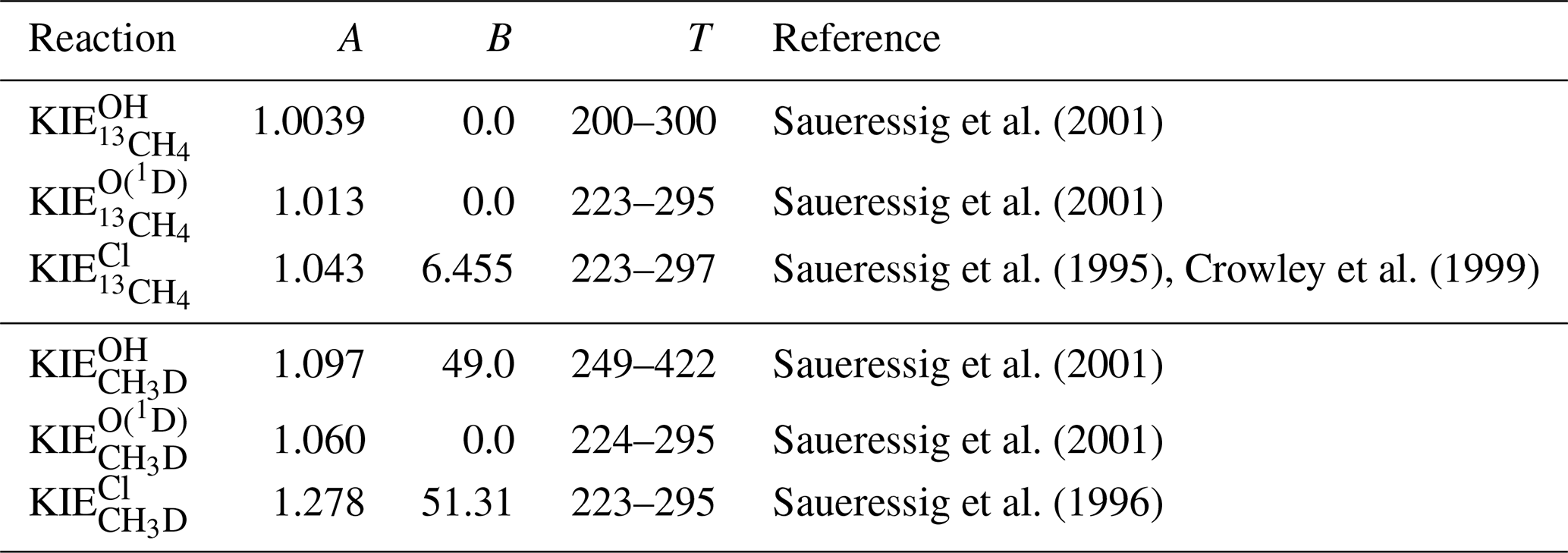
The largest KIE and therefore strongest fractionation effect is found for the reaction with Cl, which especially influences the isotopic composition of CH₄ in the middle and upper stratosphere (Saueressig et al., 1996; Bergamaschi et al., 1996). Conversely, the reaction with O(¹D) shows the lowest KIE, which furthermore does not show any temperature dependence. The KIE of the reaction with OH is temperature dependent with respect to deuterated methane (CH₃D) but not with respect to methane containing ¹³C (¹³CH₄) (Saueressig et al., 2001). Nair et al. (2005) estimated the rate coefficients of the photodissociation of CH₄ and its major isotopologues for the planet Mars, which results in a calculated KIE=1.005 for CH₃D and a negligible isotopic fractionation for the ¹³C isotopologue (Nixon et al., 2012). There is, especially for deuterium, a non-negligible fractionation during the soil-loss for CH₄ (Snover and Quay, 2000; Maxfield et al., 2008). An average value for the overall soil loss is estimated as KIE${}_{{\mathrm{CH}}_{\mathrm{3}}\mathrm{D}}^{\text{soil}}=\mathrm{1.0825}$ and KIE${}_{{}^{\mathrm{13}}{\mathrm{CH}}_{\mathrm{4}}}^{\text{soil}}=\mathrm{1.0196}$ (Snover and Quay, 2000; Holmgren, 2006; Maxfield et al., 2008).

2 The Modular Earth Submodel System (MESSy)

The framework of the Modular Earth Submodel System (MESSy, used in the second version MESSy2, Jöckel et al., 2010) is based on the idea of modularizing a climate model in such a way that single components can be switched on and off independently, depending on the desired set-up, meeting the demands of current Earth system modelling in terms of flexibility and computational performance. The modularization enables the user to pick suitable submodels or easily expand the model with new ones. Presented here are the submodel CH4 and the auxiliary submodel TRacer SYNChronization (TRSYNC), which are implemented based on this framework.

For the application examples of the new submodels, MESSy is used together with the fifth-generation European Centre Hamburg general circulation model (ECHAM5, Roeckner et al., 2006). The ECHAM/MESSy Atmospheric Chemistry (EMAC) model is a numerical chemistry and climate simulation system that includes sub-models describing tropospheric and middle atmosphere processes and their interaction with oceans, land, and human influences (Jöckel et al., 2010). EMAC (ECHAM5 version 5.3.02, MESSy version 2.54, Jöckel et al., 2010, 2016) is applied in the given examples in the T42L90MA-resolution, i.e. with a spherical truncation of T42, which corresponds to a quadratic Gaussian grid of approx. 2.8 by 2.8^∘ in latitude and longitude and includes 90 vertical hybrid pressure levels from the Earth surface up to 0.01 hPa. MESSy allows the configuration of EMAC in several operational modes. The two basic ones are the GCM set-up without chemistry and the CCM set-up with fully interactive chemistry, using, among other components, the Module Efficiently Calculating the Chemistry of the Atmosphere (MECCA, Sander et al., 2005) and the SCAVenging (SCAV, Tost et al., 2006) submodel to represent the chemical kinetics of EMAC in the gas phase and aqueous phase, respectively. They define the underlying chemical reaction mechanisms in troposphere, stratosphere, and lower mesosphere. MECCA and SCAV provide comprehensive mechanisms, combining state-of-the-art reactions and rate coefficients. The kinetic chemistry tagging technique (MECCA_TAG, Gromov et al., 2010) enables the user to tag selected chemical elements, without modifying the underlying standard chemical mechanism of MECCA. It can be applied for simulating isotopologues of trace gases with respect to selected isotopes. In order to do so, rare and abundant isotopologues of the species of interest (e.g. those containing atomic hydrogen, H) are created in an extended set of reactions in the same chemical mechanism.

MESSy and its application in EMAC has been used in multiple studies (see the special issue of Atmospheric Chemistry and Physics https://www.atmos-chem-phys.net/special_issue22.html, last access: 18 January 2021) and includes several submodels from contributing institutions. Further information on EMAC, MESSy, and its submodels can be found in Jöckel et al. (2010, 2016), on the website https://www.messy-interface.org/ (last access: 18 January 2021), or in the accompanying papers documenting the specific submodels.

3 The submodel CH4

The MESSy submodel CH4 aims to close the gap between the operational modes of EMAC as a GCM without chemistry and as a CCM with the comprehensive chemical mechanisms of MECCA and SCAV. The basic concept of the submodel is to limit the chemical mechanism to the loss processes of methane and use predefined fields of the reaction partners OH, O(¹D), and Cl to reduce the computational demands.

The sink Reactions (R1)–(R4) in the CH4 submodel are parameterized as follows:

$$\begin{array}{ll}{\displaystyle }& {\displaystyle \frac{\mathrm{d}\left[{\mathrm{CH}}_{\mathrm{4}}\right]}{\mathrm{d}t}}=(-k_{{\mathrm{CH}}_{\mathrm{4}}+\mathrm{OH}}\cdot c_{\text{air}}\cdot [\mathrm{OH}]\\ {\displaystyle }& {\displaystyle }-k_{{\mathrm{CH}}_{\mathrm{4}}+\mathrm{O}{(}^{\mathrm{1}}\mathrm{D})}\cdot c_{\text{air}}\cdot \left[\mathrm{O}{(}^{\mathrm{1}}\mathrm{D})\right]\\ \text{(3)}& {\displaystyle }& {\displaystyle }-k_{{\mathrm{CH}}_{\mathrm{4}}+\mathrm{Cl}}\cdot c_{\text{air}}\cdot \left[\mathrm{Cl}\right]-j_{{\mathrm{CH}}_{\mathrm{4}}+h\mathit{\nu }})\cdot [{\mathrm{CH}}_{\mathrm{4}}],\end{array}$$

where [X] denotes the mixing ratio of species X in mol mol⁻¹, c_air is the concentration of air in cm⁻³, k_R is the reaction rate coefficient of reaction R in cm³ s⁻¹, and $j_{{\mathrm{CH}}_{\mathrm{4}}+h\mathit{\nu }}$ is the photolysis rate of CH₄ in s⁻¹.

The prescribed fields are taken either from existing simulation results with detailed chemistry, or from other data sources (e.g. reanalyses or projections). If CH4 is included in an EMAC CCM simulation (which is possible in the MESSy framework), the CH4 submodel can also be coupled to the reactant fields, which are calculated online during the same simulation by the chemical mechanism (i.e. MECCA). Although this does not reduce computational requirements, such a simulation configuration can be used, for example, if output of one of the additional options of the CH4 submodel (age and emission classes or isotopologues) is desired. In that case a second CH₄ tracer is treated and oxidized by the reactants provided by the kinetic solver of the comprehensive chemical mechanism. The same applies for the photolysis rate of CH₄, which can be prescribed as gridded data provided offline or calculated online by the submodel JVAL (Sander et al., 2014). In either case, the CH4 submodel does not alter the reactant educts. Hence there is no feedback onto the CH₄ sink by the submodel. In the case of coupling to MECCA via the educts, the coupling is one-way only.

Figure 1 visualizes the conceptual differences between the MESSy submodel CH4 (left) and a CCM simulation with MECCA (right). MECCA simulates the entire chemical mechanism and therefore also includes the feedback onto the reaction partners (depicted in yellow) of CH₄. Additionally, there is also a secondary feedback by the products from the CH₄ sink reactions (e.g. H₂O and HO₂, depicted in blue), as the subsequent chemical processes are influenced by the products from the CH₄ oxidation. Conversely, the CH4 submodel uses the prescribed fields of the reactant species to calculate the CH₄ loss. This loss is included in the master tracer of the CH4 submodel (the present CH₄ is reduced) but does not feed back onto the sink fields or any other chemical species. The only exception is H₂O, in the case when the hydrological feedback of CH₄ oxidation is switched on. GCMs include CH₄ foremost for its radiative impact as a greenhouse gas but also for its influence on SWV (e.g. Monge-Sanz et al., 2013; ECMWF, 2007; Austin et al., 2007; Boville et al., 2001; Mote, 1995). The CH4 submodel is therefore equipped with an optional feedback onto H₂O to account for part of the secondary climate feedback of CH₄. It is thereby assumed that two molecules of H₂O are produced per oxidized CH₄ molecule (le Texier et al., 1988), which is, however, only a rough approximation, as analysed by Frank et al. (2018). The approximation of two molecules H₂O per oxidized CH₄ molecule overestimates the H₂O production in the lower stratosphere and underestimates the production in the upper stratosphere. It also does not account for the chemical loss of H₂O in the mesosphere.

Note that soil loss is not explicitly included in the CH4 submodel, since the concept of dry deposition is already part of the EMAC submodel DDEP (Kerkweg et al., 2006a). An example of how to use DDEP to simulate the soil loss of CH₄ is included in the Supplement to this paper.

The submodel CH4, with its four sink reactions of CH₄, is considerably computationally cheaper compared to a fully interactive chemistry simulation using MECCA, which represents (depending on the chosen set-up) several hundred reactions (e.g. more than 300 in the base simulations of the Earth System Chemistry integrated Modelling (ESCiMo) project Jöckel et al., 2016). For example, a reference set-up with MECCA requires about 250 node-h¹ per simulated year, while a set-up with the CH4 submodel without MECCA requires only 30 node-h per year. These numbers are calculated for simulations conducted on the high-performance computer (HPC) Mistral at the German Climate Computing Center (Deutsches Klimarechenzentrum, DKRZ).

The presented framework of the reduced CH₄ chemistry is applicable since CH₄ is only reduced and not produced in the free atmosphere. Therefore, the discretization of the four reactions where CH₄ is involved is sufficient to represent the chemical loss of CH₄. Nevertheless, in order to achieve meaningful simulation results with the CH4 submodel, some prerequisites have to be met. Since the educts (OH, O(¹D), and Cl) are prescribed, there is no feedback on them. Thus, very large variations in CH₄ mixing ratio, which would in reality influence the CH₄ sink (Winterstein et al., 2019), are not representable by the CH4 submodel.

Furthermore, the set-up with the CH4 submodel also lacks any feedback on O₃. In the atmosphere, the O₃ chemistry is influenced by changes in OH (reduced by CH₄), H₂O (produced by CH₄) and temperature (influenced by the radiatively active CH₄). The CH4 submodel alters H₂O and with that influences the radiation budget and hence the temperature; however, there is no feedback on O₃ when the set-up does not include any other chemical mechanism. In a set-up where the CH4 submodel is not used in parallel to MECCA, O₃ time series or climatologies are usually prescribed for the radiation scheme.

The first simulations using the CH4 submodel are presented in studies by Eichinger et al. (2015a, b), it was included in the simulations of the ESCiMo project (Jöckel et al., 2016), and it has been used for the CH₄ forecast system presented by Nickl et al. (2020).

3.1 Option I: age and emission classes

The CH₄ submodel includes an option for simulating age and emission classes. These classes, which can be specified by the user via a namelist, enable a precise distinction between CH₄ source sectors and/or regions (emission classes), as well as further insight into the CH₄ distribution over time (age classes). The term “emission class” thereby denotes a CH₄-like tracer defined by the CH4 submodel. The assignment of specific emission fluxes (sectors and regions) to the tracers of the emission classes is handled by the submodel OFFEMIS (Kerkweg et al., 2006b). In our present example application these classes are subject to emissions being a combination of an emission sector (like wetlands, biomass burning, anthropogenic sources, etc.) and a region (e.g. continents or countries). One tracer, for example, thus traces anthropogenic CH₄ emitted from Africa, as shown in Sect. 5.1. These additional diagnostic tracers are transported identically to the master CH₄ tracer of the CH4 submodel and also experience the same sink reactions.

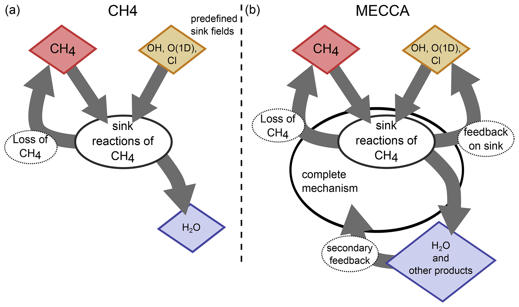
Figure 1 Sketch visualizing the concepts of parameterizing CH₄ sink reactions in the MESSy submodels CH4 (a) and MECCA (b). The red species is the core species CH₄. The chemical mechanism in CH4 is reduced to the sink reactions of CH₄ and optionally includes the feedback to H₂O (blue) only. In MECCA a complete chemical mechanism is included, which among others feeds back onto H₂O and other products of the CH₄ sink reactions, including the reaction partners (educts) of CH₄. The reaction partners (yellow) in the CH4 submodel are prescribed and not changed by the CH4 submodel.

Figure 2 Sketch showing the advancing of the age classes in the CH4 submodel. Each tracer represents one specific emission and age class. After the defined length of time, the age classes proceed to the next “older” age class. The last class represents the background CH₄, where the CH₄ is only subject to transport and the chemically defined sink reactions but is not propagated to an older age class, which is indicated by the circled arrow.

Figure 3 Sketch showing the coupling of the hydrological cycle and the chemistry (either CH4 or MECCA) with respect to H₂O isotopologues in one time step of EMAC. Green stars indicate the points of the hydrological cycle, where (1) the current value of the water vapour master tracer is taken and (2) the chemical tendencies are added onto the water vapour master tracer. Red triangles indicate the synchronization points of the corresponding isotopical tracers by the TRSYNC submodel. Synchronization of the isotopological cycles also accounts for the appropriate unit conversion and adds the tendency of chemical processes to the fractionation in the physical hydrological cycle.

The time period represented by one age class can be chosen by the user. How the age and emission classes evolve over time is depicted in Fig. 2. CH₄ of each emission class is propagated through a specific number of age classes. The emitted CH₄ of a specific emission class is added to the tracer that corresponds to the first age class. After the selected time span it moves to the next “older” age class until it reaches the oldest. The oldest age class represents the background, since CH₄ does not proceed further.

Which age evolving method is applied is also selectable. The CH4 submodel offers three options: (1) CH₄ is passed on in one step after a user-defined time span, (2) CH₄ is continuously passed on with respect to an user-defined time span, and (3) CH₄ is passed on monthly with fixed time lag.

We define the state vector for emission class i and age classes 1 to N as follows:

$$\begin{array}{}\text{(4)}& {\displaystyle }{\displaystyle }{\mathit{f}}_i=\left(\begin{array}{c}{f}_{i\mathrm{1}}\\ f_{i\mathrm{2}}\\ \mathrm{⋮}\\ f_{iN}\end{array}\right).\end{array}$$

The first two options are implemented according to

$$\begin{array}{}\text{(5)}& {\displaystyle }{\displaystyle }\mathrm{\Delta }{\mathit{f}}_i={\displaystyle \frac{\mathbf{M}\cdot {\mathit{f}}_i}{\mathrm{\Delta }t}},\end{array}$$

with Δf_i being the tendency of f_i, Δt being the time step length, and M being a matrix defining the ageing step according to the chosen option. For option (1) this matrix looks like

$$\begin{array}{}\text{(6)}& {\displaystyle }{\displaystyle }\mathbf{M}=\left(\begin{array}{cccccc}-\mathrm{1}& \mathrm{0}& & \mathrm{\cdots }& & \mathrm{0}\\ \mathrm{1}& -\mathrm{1}& & & & \\ & \mathrm{1}& -\mathrm{1}& & & \mathrm{⋮}\\ & & & \mathrm{\ddots }& \mathrm{\ddots }& \\ \mathrm{0}& & \mathrm{\cdots }& & \mathrm{1}& \mathrm{0}\end{array}\right).\end{array}$$

This moves the current values of one age class tracer after a user-defined time span to the next older one. This option is not consistent with a Leapfrog time stepping using an Asselin filter and might cause numerical oscillations and negative values. It was implemented solely for testing purposes during development, but it is not recommended for real applications. The ageing step matrix M for option (2) is M^′:

$$\begin{array}{}\text{(7)}& {\displaystyle }{\displaystyle }{\mathbf{M}}^{\prime }=\mathit{\alpha }\cdot \mathbf{M},\end{array}$$

with $\mathit{\alpha }=\frac{\mathrm{\Delta }t}{\stackrel{\mathrm{̃}}{T}}$ and $\stackrel{\mathrm{̃}}{T}$ being the user-defined time span indicating the binning width of the age class. This option carries out a quasi-continuous update of the age classes, as it moves a fraction (α) of the current age class to the next at every time step.

The third option is implemented for usage by a fixed-lag Kalman filter for inverse optimization. With this option, one age class represents 1 month, and at the end of 1 month all CH₄ of one age class moves to the next. This option is specifically implemented to be consistent with the Leapfrog time stepping (cf. option 1). A preliminary application of the concept of using the age and emission classes for an inverse optimization using the fixed-lag Kalman filter has been shown by Frank (2018).

In order to reduce numerical errors, the age and emission classes are continuously constrained (i.e. in each model time step) to sum up to the master tracer and are scaled appropriately if the sum deviates. This procedure is done to avoid the accumulation of such numerical errors, which mainly arise from small non-linearities in the large-scale advection scheme. The magnitude therefore depends on the applied advection scheme but is usually on the order of the floating point precision.

3.2 Option II: isotopologues

In addition to solving the basic CH₄ kinetics, the submodel CH4 also allows for the simulation of CH₄ isotopologues, which are a potent diagnostic measure in the source and sink attribution. The submodel CH4 is able to simulate the abundant and first-order rare isotopologues and defines these as tracers additional to the master tracer. Higher substituted isotopologues are neglected. The user can choose whether isotopologues are simulated with respect to carbon (¹²CH₄ and ¹³CH₄), hydrogen (CH₄ containing ¹H isotopes only and CH₃D), or both. The abundant (with ¹²C or ¹H isotopes only) and rare (with ¹³C or D) isotopologues are thereby simulated in parallel. During the simulation care is taken that each isotopologue family sums up to the master CH₄ tracer of the CH4 submodel (CH4_fx). The isotopic signatures of CH₄ emission sources are included by splitting the emission fluxes into an abundant and a rare fraction. This is handled via the OFFEMIS namelist (Kerkweg et al., 2006b; see the example namelists in the Supplement).

The rate coefficients of the CH₄ isotopologues with their reaction partners are adjusted with respect to the KIE factors, e.g.

$$\begin{array}{}\text{(8)}& {\displaystyle }{\displaystyle }\text{KIE}=k_{{\text{CH}}_{\mathrm{4}}+\text{OH}}/k_{{\text{CH}}_{\mathrm{3}}\mathrm{D}+\text{OH}},\end{array}$$

and are similar for reactions with O(¹D), Cl, and photolysis. The applied reaction partners are thereby the same as those used for the master tracer.

To a certain extent the oxidation of CH₃D produces deuterated water vapour (HDO). If the feedback of CH₄ oxidation onto the hydrological cycle and the simulation of D-containing isotopologues is switched on in the CH4 submodel, an additional tracer for HDO is created by the submodel and filled by the produced HDO from CH₃D oxidation. There are two options available: (1) one oxidized CH₃D produces one HDO molecule, or (2) the tendency of the HDO tracer is calculated by Eq. (9) (Eichinger et al., 2015a):

$$\begin{array}{}\text{(9)}& {\displaystyle }{\displaystyle \frac{\partial \left(\text{HDO}\right)}{\partial t}}={\displaystyle \frac{-\frac{\partial \left({\mathrm{CH}}_{\mathrm{3}}\mathrm{D}\right)}{\partial t}+\mathrm{6.32}\times {\mathrm{10}}^{-\mathrm{5}}\cdot \frac{\partial \left({\mathrm{CH}}_{\mathrm{4}}\right)}{\partial t}}{\frac{M_{\text{air}}}{M_{\text{HDO}}}{\left(\frac{\mathrm{1}}{\mathrm{1}-\text{HDO}}\right)}^{\mathrm{2}}}},\end{array}$$

with M_air and M_HDO being the molar masses of air (28.987 g mol⁻¹) and HDO (19.02 g mol⁻¹), respectively. This empirical equation accounts for the D, which stays in molecular hydrogen (HD) as it builds up to an equilibrium with HDO via the HO_x cycle.

4 Coupling to the hydrological cycle with the new submodel TRSYNC

In EMAC three different submodels are included that deal with isotopologues of H₂O in the vapour phase: (1) the CH4 submodel presented here, (2) MECCA_TAG, and (3) H₂O ISOtopologues (H2OISO, Eichinger et al., 2015a). CH4 and MECCA_TAG include the chemical fractionations, while H2OISO is responsible for the physical fractionations in the hydrological cycle of the underlying GCM. All three create independent tracers of H₂O isotopologues, which need to be synchronized to be able to combine physical and chemical fractionation effects of H₂O and its isotopologues. The chemical fractionation is thereby considered either from MECCA_TAG or from CH4, although both submodels can be concurrently included in a simulation and compute the isotopic fractionation independently.

In principle, if EMAC is applied in GCM mode, only the master hydrological cycle is present (see Fig. 3, inner blue circle). Adding MECCA or CH4 to the set-up expands the model into a CCM or a simple “CH₄-only” CCM, respectively (solid red circle). The chemistry submodels use water vapour as a chemical tracer (first green star) and calculate the contribution from CH₄ oxidation (second green star). This chemical feedback onto water vapour was already implemented as an option in previous EMAC versions. By including the isotopological submodels into the set-up, H2OISO duplicates the hydrological cycle for the water isotopologues and CH4 or MECCA_TAG creates the chemical tracers of the water isotopologues (outer dashed circles). This results in several physical and chemical H₂O isotopologue tracers. While the master chemical process adds its feedback directly to the specific humidity of the hydrological cycle (there is no need for a chemical water tracer), the synchronization of the physical isotopological tracers in the isotopic hydrological cycle (H2OISO) and the chemical isotopological tracers (CH4 or MECCA_TAG) is done via the new auxiliary submodel TRSYNC. In brief, TRSYNC guarantees that the physical H₂O tracers (including their isotopologues) also receive the correct tendencies of the corresponding chemical tracers. Since isotopological water vapour tracers of MECCA_TAG and the HDO tracer created by CH4 are transported in EMAC in the same way as every other tracer, they are subject to some of the physical processes but not to all hydrological fractionation effects. Thus, at the first synchronization point the chemical tracer is synchronized to represent the current value of the physical tracer. In the following, chemical tendencies including fractionation effects are calculated and are added via the second synchronization point to the physical tracer. By doing so, chemical and physical fractionation processes are strictly separated and the tendencies of the chemical tracers represent the chemical tendencies in addition to the previous physical fractionations in the current time step.

Water vapour in the physical hydrological cycle (regarding ECHAM5 and H2OISO) is defined in units of kilograms of the tracer per kilogram of moist air (${\mathrm{kg}{\mathrm{kg}}^{-\mathrm{1}}}_{\text{moist air}}$), while the chemical tracers are defined in units of ${\mathrm{mol}{\mathrm{mol}}^{-\mathrm{1}}}_{\text{dry air}}$. This also holds for the corresponding isotopologue tracers. Parameterizations of physical processes in ECHAM5 are by design formulated with specific humidity (per moist air). Conversely, chemical reactions are necessarily calculated with species concentrations. This requires the individual chemical and physical isotopologue tracers, which have, for the sake of correct process formulations, distinct units, and motivated the development of the auxiliary submodel TRSYNC in order to be able to synchronize these tracers accordingly in the same way for CH4 and MECCA_TAG.

In addition to that, the application of MECCA_TAG creates the basis to investigate various other isotopes in the interactive chemical mechanism. While CH4 feedbacks onto H₂O with respect to hydrogen isotopes only, MECCA_TAG can also be used to simulate oxygen isotopes (¹⁶O, ¹⁷O and ¹⁸O) in the chemical mechanism. It is therefore also possible to couple MECCA_TAG with oxygen isotopes to the corresponding oxygen-related isotopologue tracers in H2OISO. Last but not least, for MECCA_TAG tracer names are not standardized. Therefore, the namelist of the submodel TRSYNC can be adjusted according to the actual tracer names used in MECCA_TAG.

5 Example applications

The following examples are simulations carried out with EMAC in a GCM-like mode, including the newly presented CH4 and TRSYNC submodels. Other involved MESSy submodels are OFFEMIS (Kerkweg et al., 2006b) and DDEP (Kerkweg et al., 2006a). OFFEMIS manages the emissions of CH₄ from prescribed sources. It reads predefined fields with emission data and adds these fluxes to the chemical tracers. DDEP simulates the dry deposition for gases and aerosols and is used in the present context to simulate the soil loss of CH₄, which is not done in the CH4 submodel itself.

Monthly mean sink fields are used in the simulation set-up in the examples below. Higher frequencies are technically possible; this would, however, increase the computational demands due to the larger amount of data read from disk. Monthly mean fields smooth the diurnal cycle, which is especially strong in OH. However, in order to investigate long-term global trends of CH₄, which has a tropospheric lifetime of 8–10 years, variations on timescales of less than 1 month are negligible, and monthly mean fields are assumed to suffice for such applications. Furthermore, in these examples photolysis rates are calculated by the submodel JVAL in the presented examples, but predefined data can be used as well.

The H2OISO submodel (Eichinger, 2014; Eichinger et al., 2015a) simulates the stable water isotopologues with respect to H and D, as well as ¹⁶O, ¹⁷O, and ¹⁸O. Overall, it represents a second hydrological cycle, which includes water isotopologues in their three phases: gas, liquid, and ice. H2OISO accounts for fractionation processes during phase transitions in large-scale and convective clouds, during vertical diffusion, and during evaporation from the ocean (evaporation from soil, the biosphere, and snow are not considered to have a significant fractionation).

We simulated the years 1989 to 2012 and applied a specified dynamics set-up to represent the reanalysed meteorology of this time. Specified dynamics means here that the prognostic variables divergence, vorticity, temperature, and (logarithm of) surface pressure are nudged by Newtonian relaxation towards ECMWF ERA-Interim reanalysis data (Dee et al., 2011).

5.1 Application of the CH4 submodel for inverse optimization of CH₄ emission inventories

Current estimates of CH₄ emission inventories still include large uncertainties. In order to reduce these, new estimates of inventories must be able to represent temporal and spatial resolutions in greater detail (e.g. seasonal cycle, distinct regions). One statistical method to estimate CH₄ emission strengths is the fixed-lag Kalman filter, which performs an inverse optimization of the emission inventory by comparing simulated and observed mixing ratios of a trace gas (see, e.g. Bruhwiler et al., 2005). This “offline” inversion algorithm requires data from a forward simulation, including temporal and spatial information of the simulated CH₄ tracer.

In order to provide the necessary data, the CH4 submodel with the option of age and emission classes is applied. The combination of chosen regions and emission sectors in this example results in 48 emission classes altogether. These 48 emission classes are simulated with 5 age classes for ages up to 1, 2, 3, 4, and ≥5 months since emission release. Figure 4 exemplarily shows the evolution of a single emission class (i.e. anthropogenic emissions in Africa) from age class to age class. Figure 4a shows the emissions of the year 2000 in g(CH₄) ${\mathrm{m}}^{-\mathrm{2}}{\mathrm{yr}}^{-\mathrm{1}}$. Figure 4b–f show the age classes in ascending order and display the distribution of the CH₄ mixing ratio onto the five age classes in January 2000 (the simulation has started in 1989). In the fourth age class the CH₄ from anthropogenic African sources is almost evenly distributed, mostly in the Northern Hemisphere (NH). Eventually, the fifth age class (i.e. the last age class) shows the accumulated background of all CH₄ from anthropogenic African sources. An a priori emission inventory is applied in the example situation.

Overall, the temporal evolution of the age classes in Fig. 4 confirms that the five age classes in this set-up sufficiently track the spread of CH₄ towards a fairly uniform distribution, which is a prerequisite for a successful application of the inverse optimization method.

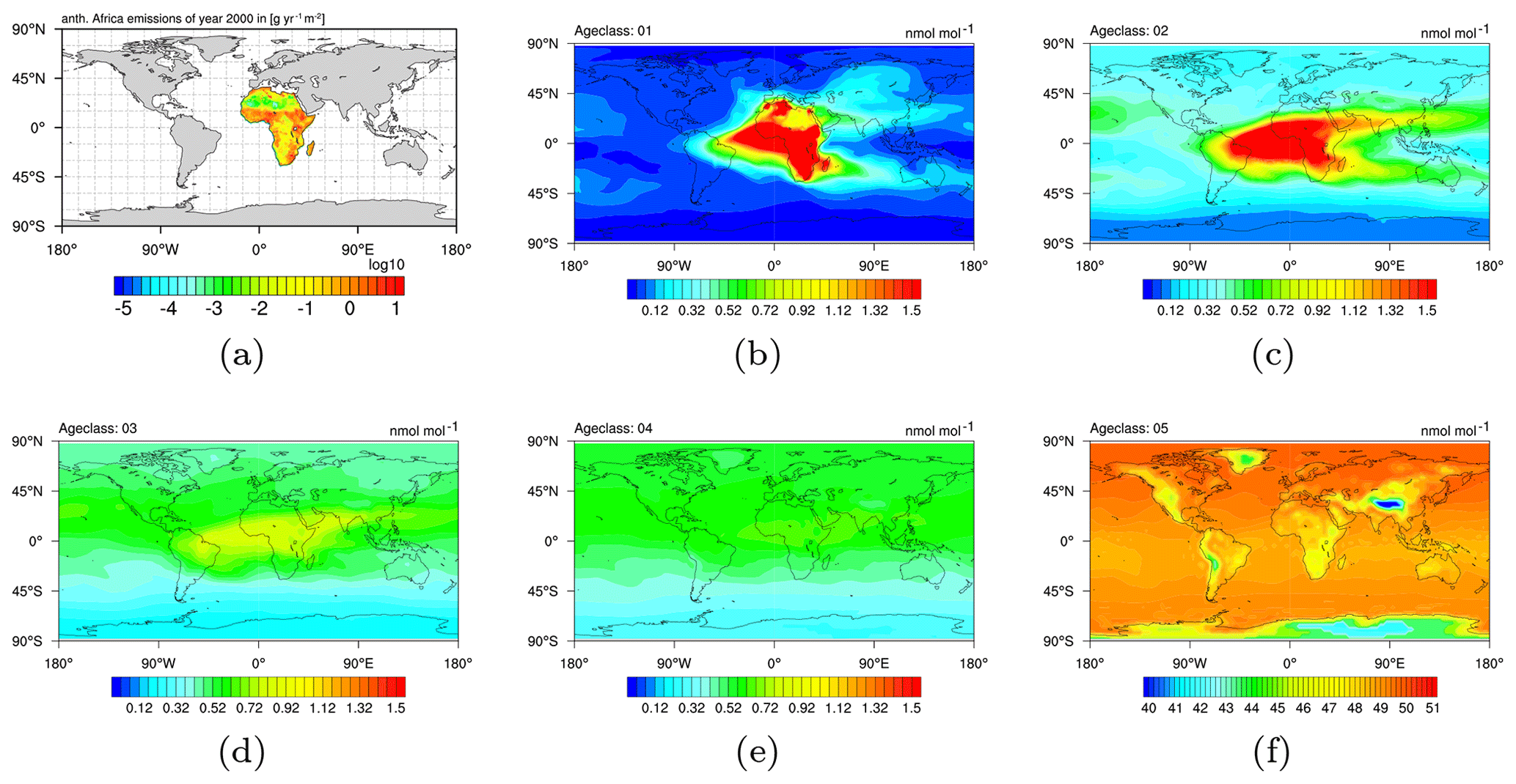
Figure 4 (a) Anthropogenic emissions in Africa (taken from EDGARv4.2 2010 fast-track database; Olivier and Janssens-Maenhout, 2012). (b–f) Methane as a pressure-weighted column up to 200 hPa of anthropogenic origin from Africa, distributed into five age classes, i.e. up to 1, 2, 3, and 4, and ≥5 months after emission release. As an example, all age classes of January 2000 after the simulation has run for 12 years are shown.

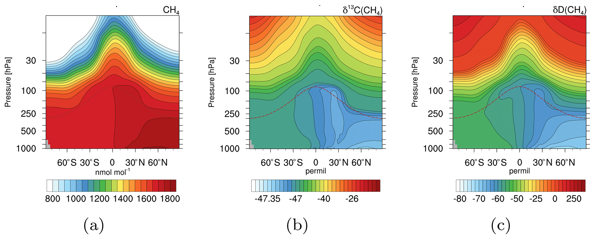
Figure 5 Zonal mean climatologies of 2000–2009 for CH₄ in nmol mol⁻¹ (a), δ¹³C(CH₄) in ‰ (b), and δD(CH₄) in ‰ (c) of the simulation with EMAC and the CH4 submodel. The dashed brown lines indicate the height of the climatological tropopause.

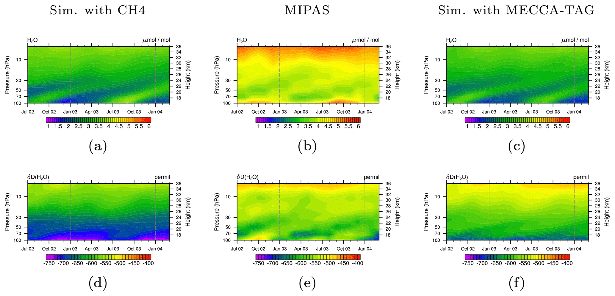
Figure 6 Tropical stratospheric tape recorder signal of H₂O (a, b, c) and δD(H₂O) (d, e, f) in MIPAS data (b, e) and the simulations with the CH4 submodel (a, d) and the MECCA_TAG submodel (c, f) in the time period July 2002 to March 2004. Simulation data are averaged monthly, zonally, and over the tropics between 23^∘ S–23^∘ N and are displayed between 100 and 1 hPa. The dashed grey lines are included for eye guidance in the comparison of the tape recorder signal.

5.2 Simulating CH₄ isotopologues

We further present a simulation using the CH4 submodel, which includes all four CH₄ isotopologues. For this simulation, we applied a global a posteriori emission inventory provided by Dominik Brunner (personal communication, 2017) and a set of isotopic emission signatures prepared from data from the literature (see Table S1 in the Supplement).

Figure 5 shows zonal mean climatologies (2000–2009) of CH₄ in nmol mol⁻¹ and the corresponding isotopic signature in ‰. The isotopologues are displayed in the δ notation with respect to the reference isotope ratios Vienna PeeDee Belemnite (VPDB) for ¹³CH₄, and Vienna Standard Mean Ocean Water (VSMOW) for CH₃D, respectively. In the troposphere the NH is isotopically depleted compared to the Southern Hemisphere (SH). Most isotopically light emissions, for example from wetlands and rice, are located in the NH, while isotopically heavy sources like biomass burning are mostly located in the SH. This results in the prevalent tropospheric north–south gradient. In the stratosphere CH₄ becomes isotopically enriched towards higher altitudes. When CH₄ is ascending in the atmosphere it is exposed to oxidation. Due to fractionation processes, heavy CH₄ isotopologues are unfavoured and therefore accumulate in the remaining CH₄.

Our simulation results compare well to observations. For example, isotopic observations from the National Oceanic and Atmospheric Administration/Earth System Research Laboratory (NOAA/ESRL) sampling sites (White et al., 2016, 2017) and airborne samples taken during the Comprehensive Observation Network for TRace gases by AIrLiner (CONTRAIL) project (Umezawa et al., 2012) verify the north–south gradient (shown Sect. S2.1 and S2.2 in the Supplement). The values of the signature of ¹³C in CH₄ (δ¹³C(CH₄)), for example, are within the uncertainty of the CONTRAIL observations. The signature of D in CH₄ (δD(CH₄)) is isotopologically depleted in D compared to the CONTRAIL observations; however, it still captures the gradient well. The vertical gradient (i.e. isotopical enrichment in the stratosphere) can be verified by comparing it with balloon-borne observations by Röckmann et al. (2011). Our simulation results are thereby within the local and temporal uncertainties (shown in Sect. S2.3 in the Supplement). Note that an optimization with respect to source signatures is yet to be made and requires an optimized emission inventory. However, the capturing of the respective gradients indicates that the isotopical fractionation is sufficiently implemented.

5.3 Coupling of the CH₄ isotopologues to the isotopological hydrological cycle

The previously shown results were achieved with the CH4 submodel, including the option to simulate CH₄ isotopologues. The produced HDO (by oxidation of CH₃D) is connected via the TRSYNC submodel to the isotopological hydrological cycle represented by the H2OISO submodel. We carried out an additional simulation in which we applied MECCA and MECCA_TAG to simulate the atmospheric chemistry and the CH₄ isotopologues instead of the CH4 submodel. In this simulation TRSYNC likewise connects the produced HDO to the isotopological water tracers of H2OISO.

In Fig. 6 we compare the results obtained with submodel CH4 (left) and those obtained with the submodel MECCA_TAG (right) to vertical profiles of H₂O and HDO (middle) provided by the Michelson Interferometer for Passive Atmospheric Sounding (MIPAS) instrument mounted on the ENVIronmental SATellite (ENVISAT, Steinwagner et al., 2007; Lossow et al., 2011). The ENVISAT satellite is on a sun-synchronous orbit around the Earth, completing the circuit 14 times a day. The presented observational and simulated data comprise the time period July 2002 to March 2004. The vertical range of the observations extends from 6 to 68 km (i.e. approx. the range 100–1 hPa) with a vertical resolution of 3–8 km. Simulation and observation data are monthly and zonally averaged over the tropics. Similar to the conclusions of Eichinger et al. (2015a) it is observed that the EMAC model underestimates the H₂O mixing ratio (see Figs. 6a and c). This is associated with a too cold tropopause in EMAC, where a temperature bias of −2 to −6 K is detected in the upper troposphere, as long as the mean temperature is excluded from the nudging procedure defining the specified dynamics set-up (Jöckel et al., 2016). This reduces the H₂O transported into the stratosphere since more gas-phase H₂O freezes and sediments. Comparing Fig. 6d with f indicates a better agreement concerning the signature of D in H₂O (δD(H₂O)) in the simulation using the submodel MECCA_TAG with the MIPAS observations, which suggests that although the absolute H₂O and HDO mixing ratios are not met, the relative composition is well represented. The differences in HDO in the simulation with the CH4 submodel compared to the one with the MECCA_TAG submodel and MIPAS are potentially caused by (1) the Eq. (9) from Eichinger et al. (2015a) used in the simulation using the CH4 submodel, which possibly does not capture important fractionation processes in the oxidation chain of CH₃D, and (2) the HD produced in the troposphere and propagating into the stratosphere, which is not included in the simplified chemistry but represents an additional source of HDO. For an accurate simulation of stratospheric HDO this source also needs to be considered in future simulations.

6 Summary

The submodel CH4 provides a reduced chemical set-up focusing on the CH₄ sink reactions using predefined data of reaction partners and optionally includes the feedback on SWV. This reduces the computational demands of sensitivity simulations of climate projections without neglecting the main source of chemically induced SWV.

We present two additional options of the CH4 submodel. The age and emission classes allow the inverse optimization of emission inventories using a fixed-lag Kalman filter. The simulation of CH₄ isotopologues provides further insight into the variability and distribution of CH₄ from its source (via emission signatures and fractionation effects) to its sink (coupling to the isotopic content of H₂O). The latter is implemented in form of the new submodel TRSYNC, which takes care of the correct and time-integration-conform synchronization of the various H₂O isotopologue tracers in the model.

Example use cases show specific applications of the CH4 submodel and the coupling to the isotopological hydrological cycle via the TRSYNC submodel, which is especially helpful for the closure of the isotopic content in SWV.