Development of adjoint-based ocean state estimation for the Amundsen and Bellingshausen seas and ice shelf cavities using MITgcm–ECCO (66j)

The Antarctic coastal ocean impacts sea level rise, deep-ocean circulation, marine ecosystems, and the global carbon cycle. To better describe and understand these processes and their variability, it is necessary to combine the sparse available observations with the best-possible numerical descriptions of ocean circulation. In particular, high ice shelf melting rates in the Amundsen Sea have attracted many observational campaigns, and we now have some limited oceanographic data that capture seasonal and interannual variability during the past decade. One method to combine observations with numerical models that can maximize the information extracted from the sparse observations is the adjoint method, a.k.a. 4D-Var (4-dimensional variational assimilation), as developed and implemented for global ocean state estimation by the Estimating the Circulation and Climate of the Ocean (ECCO) project. Here, for the first time, we apply the adjoint-model estimation method to a regional configuration of the Amundsen and Bellingshausen seas, Antarctica, including explicit representation of sub-ice-shelf cavities. We utilize observations available during 2010–2014, including ship-based and seal-tagged CTD measurements, moorings, and satellite sea-ice concentration estimates. After 20 iterations of the adjoint-method minimization algorithm, the cost function, here defined as a sum of the weighted model–data difference, is reduced by 65 % relative to the baseline simulation by adjusting initial conditions, atmospheric forcing, and vertical diffusivity. The sea-ice and ocean components of the cost function are reduced by 59 % and 70 %, respectively. Major improvements include better representations of (1) Winter Water (WW) characteristics and (2) intrusions of modified Circumpolar Deep Water (mCDW) towards the Pine Island Glacier. Sensitivity experiments show that ∼40 % and ∼10 % of improvements in sea ice and ocean state, respectively, can be attributed to the adjustment of air temperature and wind. This study is a preliminary demonstration of adjoint-method optimization with explicit representation of ice shelf cavity circulation. Despite the 65 % cost reduction, substantial model–data discrepancies remain, in particular with annual and interannual variability observed by moorings in front of the Pine Island Ice Shelf. We list a series of possible causes for these residuals, including limitations of the model, the optimization methodology, and observational sampling. In particular, we hypothesize that residuals could be further reduced if the model could more accurately represent sea-ice concentration and coastal polynyas.

1 Introduction

The ice shelves and glaciers in the Amundsen Sea (AS) and Bellingshausen Sea (BS) are melting and thinning rapidly with consequences for global sea level rise and changes in ocean circulation and the global carbon cycle (e.g., Arrigo et al., 2008; Pritchard et al., 2012; Paolo et al., 2015; Bronselaer et al., 2018; Rignot et al., 2019). Basal melting of these ice shelves is caused by warm modified Circumpolar Deep Water (mCDW, 0.5–1.5 ^∘C), which intrudes onto the continental shelf towards the ice shelf cavities following submarine glacial troughs (Fig. 1) (e.g., Jacobs et al., 1996; Walker et al., 2007; Jacobs et al., 2011; Nakayama et al., 2013; Walker et al., 2013; Dutrieux et al., 2014). For this reason, multiple oceanographic observational campaigns have been collected by the international community to understand the mechanism of mCDW intrusions onto the AS continental shelf and towards ice shelf cavities. As part of these efforts, we now have some limited oceanographic data that capture seasonal and interannual variability during the past decade (e.g., Jacobs et al., 2011; Nakayama et al., 2013; Dutrieux et al., 2014; Heywood et al., 2016; Kim et al., 2017; Webber et al., 2017; Mallett et al., 2018).

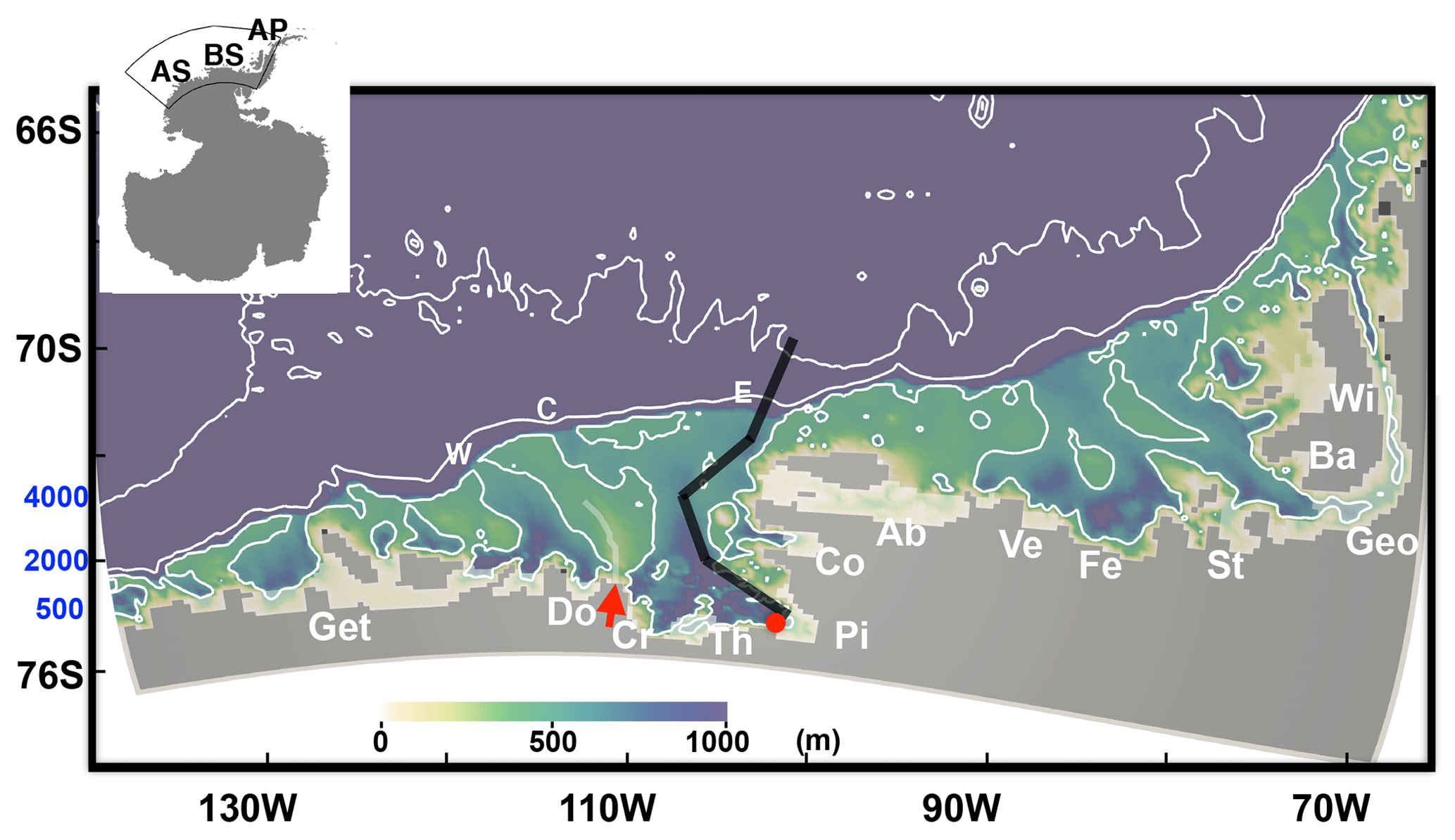
Figure 1 Model bathymetry (color) with contours of 500, 2000, and 4000 m in white. The inset (top left) shows Antarctica with the region surrounded by a black line denoting the location of the enlarged portion. AS, BS, and AP denote the Amundsen Sea, Bellingshausen Sea, and Antarctic Peninsula region, respectively. The ice shelves are indicated with transparent white-outlined patches, and abbreviations are summarized in Table 4. Letters E, C, and W denote the submarine glacial troughs located on the eastern AS continental shelf. Transparent white-outlined patches (see the red arrow between Do and Cr) indicate the location of grounded icebergs and landfast ice. This white region is treated as a barrier in the sea-ice model, and we do not allow sea-ice exchange to cross this region. The thick black line represents the vertical section shown in Figs. 4 and 5.

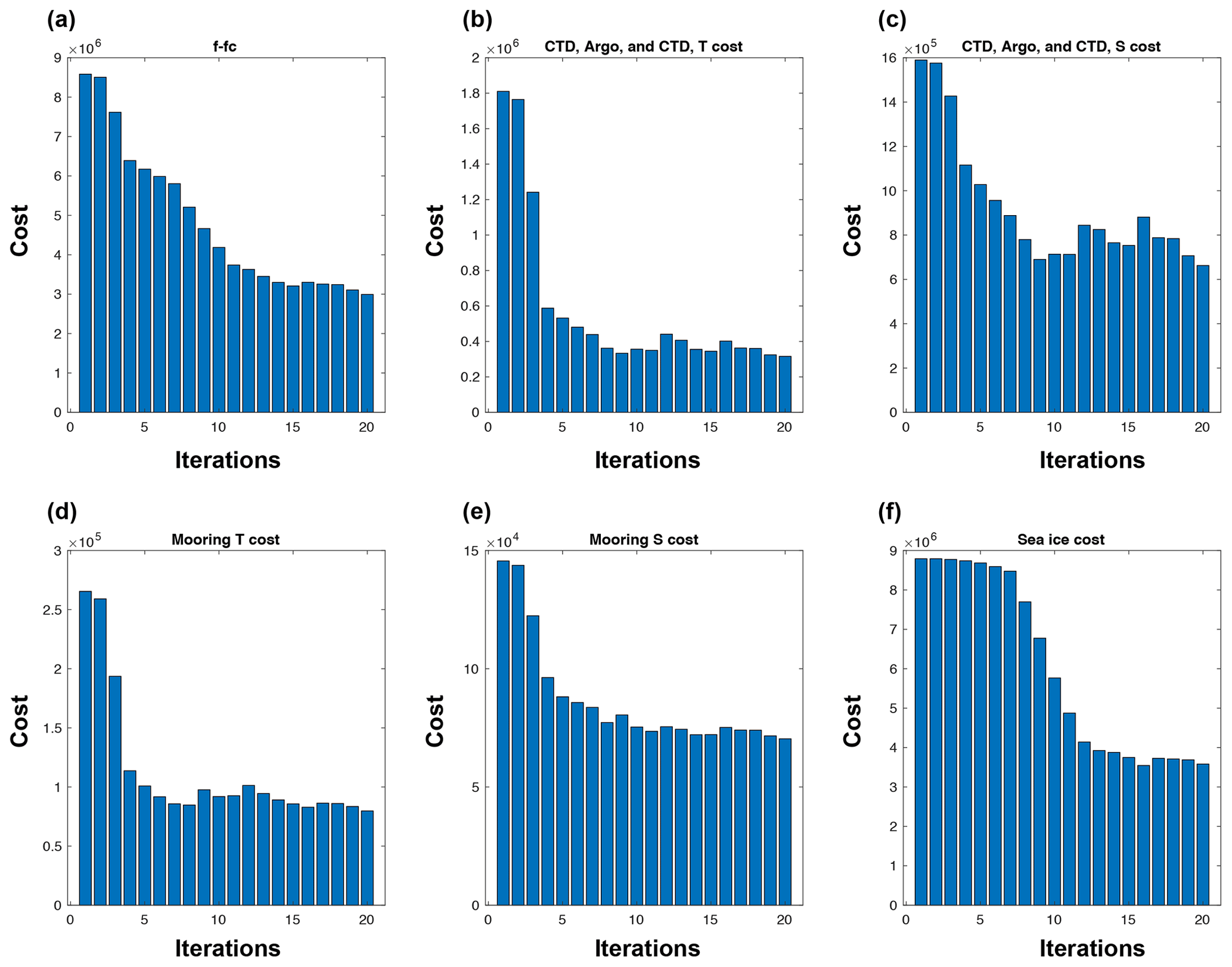
Figure 2 Evolution of (a) total; (b) ship-based, Argo, and seal-tagged CTD temperature; (c) ship-based, Argo, and seal-tagged CTD salinity; (d) mooring temperature; (e) mooring salinity; and (f) sea-ice costs. Note that vertical scales are different for all panels.

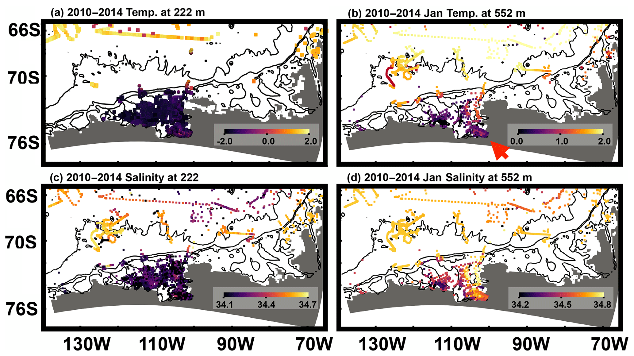
Figure 3 The (a) 222 m and (b) 552 m potential temperature used for model–data difference calculation and (c) 222 m and (d) 552 m salinity used for model–data difference calculations. Bathymetric contours of 500, 2000, and 4000 m are shown in black. The red arrow indicates the PIIS front region.

Nakayama et al. (2013)Dutrieux et al. (2014); Kim et al. (2017)Heywood et al. (2016)Ducklow et al. (2012)Webber et al. (2017)Kim et al. (2017)Mallett et al. (2018)Cavalieri et al. (1996)

Table 1 Oceanographic datasets used for ocean state estimates.

Table 2 Model parameters used for ocean simulations. Most parameters are chosen based on Nakayama et al. (2017) and Zhang et al. (2018) with some adjustments.

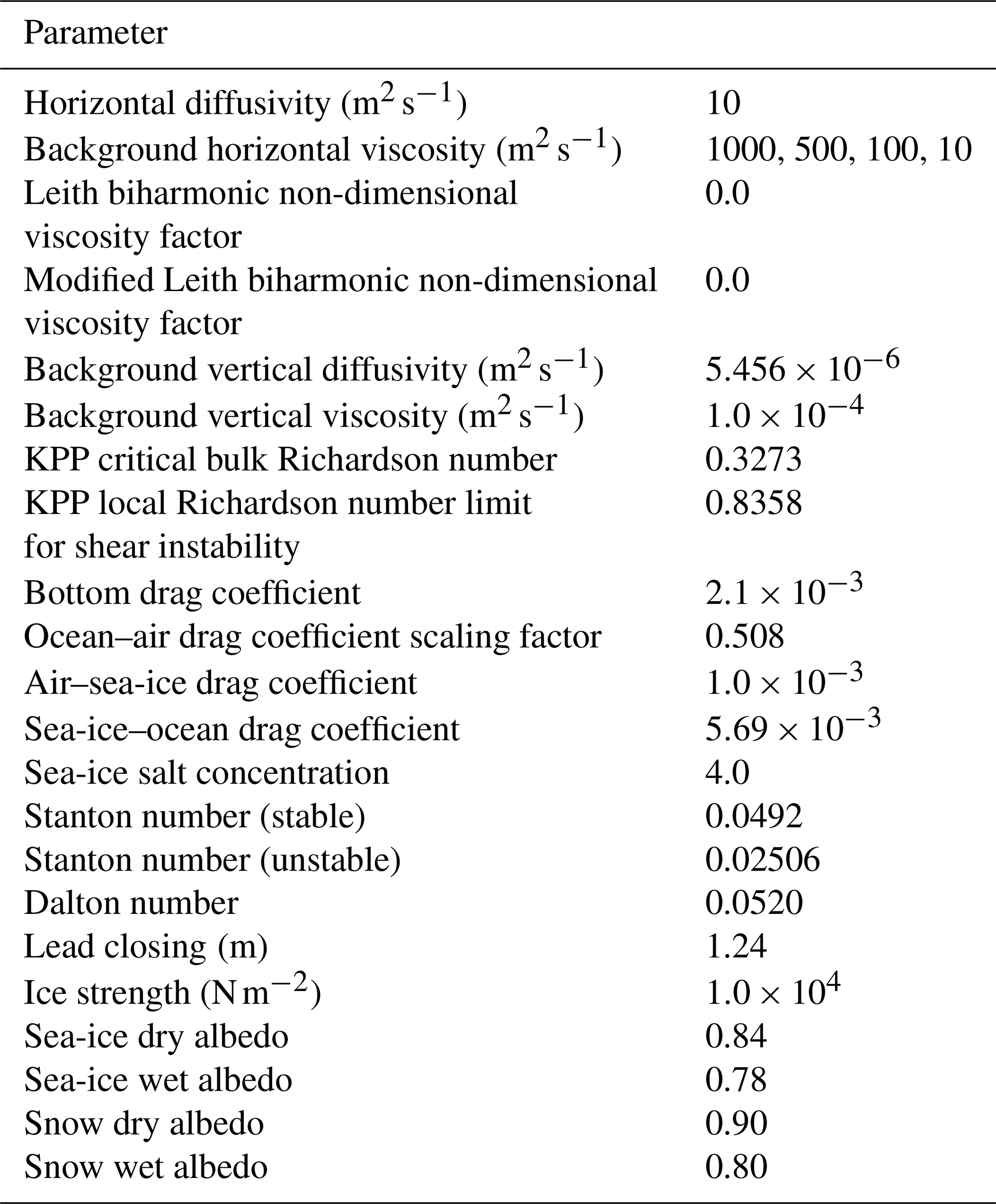
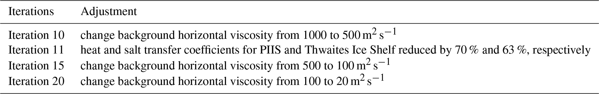
Table 3 Adjustments to model parameters in addition to optimization using adjoint sensitivities.

Recent observations as well as modeling studies reveal that mCDW pathways, ice shelf–ocean interaction, the thermocline depth, and ocean bathymetry below the Pine Island Ice Shelf (PIIS) are important for controlling the PIIS melt rate (e.g., Schodlok et al., 2012; Dutrieux et al., 2014; De Rydt et al., 2014; St-Laurent et al., 2015; Dinniman et al., 2016; Jourdain et al., 2017; Kimura et al., 2017; Webber et al., 2019). The thermocline depth was ∼200 m deeper in 2012 compared to in other years (e.g., 1994, 2007, 2009, and 2010; see Fig. 2A in Dutrieux et al., 2014), which reduced the PIIS melt by ∼50 %. After 2012, the thermocline shoaled by 200 m returning to its more commonly observed depth of ∼350 m (Webber et al., 2017). It is suggested that this thermocline variability was caused by changes in local and remote surface wind and buoyancy forcing (Dutrieux et al., 2014; Webber et al., 2017).

To better describe and understand these processes and their variability, it is necessary to combine the sparse available observations with the best-possible numerical representations of ocean circulation. One method to combine observations with numerical models that can maximize the information extracted from the sparse observations is the adjoint method, also known as 4-dimensional variational assimilation (4D-Var), as developed and implemented for global ocean state estimation by the Estimating the Circulation and Climate of the Ocean (ECCO) project. To date, the ECCO project has produced ocean state estimates based on circum-Antarctic or global model configurations (e.g., Mazloff et al., 2010; Forget et al., 2015; Zhang et al., 2018; Fukumori et al., 2020). Employing the adjoint model produced by automatic differentiation (Giering and Kaminski, 1998), a.k.a. algorithmic differentiation, and utilizing temporally varying oceanographic observations, these ocean state estimates are capable of simulating the large-scale evolution of the Southern Ocean consistent with the available observations. Many observational and modeling studies have been conducted to understand Southern Ocean gyre dynamics, subsurface ocean circulation, the southern shift of various fronts around Antarctica, etc. (e.g., Gille et al., 2016; Jones et al., 2016; Tamsitt et al., 2017; Nakayama et al., 2018; Roach and Speer, 2019; Jones et al., 2020). However, despite the importance of Antarctic coastal regions for global climate, existing models fail to accurately reproduce the sparse available observations, likely owing to the difficulty in simulating Antarctic continental shelf regions and sub-ice-shelf-cavity processes (Mazloff et al., 2010; Timmermann et al., 2012; Kusahara and Hasumi, 2013; Nakayama et al., 2014; Rodriguez et al., 2016; Nakayama et al., 2017; Kusahara, 2020).

For other regions of the globe, ocean state estimates based on regional configurations have been successfully developed during the past decades, achieving good model–data agreement and leading to understanding of regional processes (Fenty and Heimbach, 2013b, a; Verdy et al., 2014, 2017; Rudnick et al., 2015; Nguyen et al., 2020; Vinogradova et al., 2014). For Antarctic coastal regions, however, the only previous attempt to constrain a model with observations was the study of Nakayama et al. (2017), which used a low-dimension estimation approach based on the computation of model Green's functions. Here we aim to extend the study of Nakayama et al. (2017) by employing the adjoint method, which permits a larger number of higher-dimension control variables than the Green's functions approach. The objective is to obtain a closer fit to the available observations than what was achieved in Nakayama et al. (2017). This objective is challenging due to several difficulties including that (1) polar-specific processes (ice shelf and sea ice) are highly nonlinear and (2) observational data are limited. The groundwork for making adjoint-method optimization possible in the presence of ice shelf cavities was laid out in the study of Heimbach and Losch (2012), who obtained adjoint sensitivities of sub-ice-shelf melt rates to ocean circulation under the Pine Island Ice Shelf, West Antarctica.

In this study, we present our attempt at the development of Amundsen Sea–Bellingshausen Sea ocean state estimates by employing the adjoint-model-based data assimilation method developed by ECCO for regional and global ocean state estimation (Mazloff et al., 2010; Forget et al., 2015; Zhang et al., 2018; Fukumori et al., 2020). We focus on the years 2010–2014 when oceanographic observations were collected frequently and the largest interannual variability was observed (Dutrieux et al., 2014; Webber et al., 2017). Our simulations are carried out for a subregion of the global 1$/$3^∘ ECCO solution, a.k.a. ECCO LLC270 (Zhang et al., 2018). Using the ECCO LLC270 solution both provides lateral boundary conditions for this study and enables this work to be a stepping stone towards improved representation of ice shelf–ocean interactions in ECCO global ocean retrospective analyses. We note, however, that the LLC270 horizontal and vertical resolutions are insufficient to resolve critical ocean and ice shelf processes, e.g., eddy transport and mean-flow–topography interactions. Hence, these sub-grid-scale processes need to be parameterized and adjusted.

2 Data and methods

2.1 Observations

In the Amundsen Sea, oceanographic observational campaigns were carried out in 2010, 2012, and 2014 (Nakayama et al., 2013; Dutrieux et al., 2014; Heywood et al., 2016; Kim et al., 2017). Several mooring observations were also obtained, with the moorings at the PIIS front capturing the largest interannual variability observed in the region between 2009–2014 (Dutrieux et al., 2014; Webber et al., 2017). We also utilize seal-tagged CTD observations obtained in 2014, which contain over 10 000 profiles between February and November (Heywood et al., 2016). In the central part of the Bellingshausen Sea, no oceanographic observations were collected between 2010–2014. Recently, we have become aware that seal-tagged CTD observations, mostly in the Bellingshausen Sea (Roquet et al., 2013; Zhang et al., 2016), are available for inclusion in future studies. For the Antarctic Peninsula region, oceanographic observations were collected by the Palmer Antarctic Long-Term Ecological Research project (PAL-LTER; Ducklow et al., 2012). For sea ice, we use satellite-based estimates of daily sea-ice concentration with grid resolutions of 25 km (Cavalieri et al., 1996). The datasets used in this study are summarized in Figs. 2 and 3 and Table 1.

2.2 Numerical model

We employ the Massachusetts Institute of Technology General Circulation Model (MITgcm), which includes dynamic–thermodynamic sea-ice (Losch et al., 2010) and thermodynamic ice shelf (Losch, 2008) capabilities. Following the model configuration from Nakayama et al. (2017), we extract the regional grid from a global LLC270 configuration for the AS and BS regions (Fig. 1). In the AS and BS domain, horizontal grid spacing is approximately 10 km (Fig. 1). The vertical discretization of the ECCO LLC270 configuration comprises 50 levels varying in thickness from 10 m near the surface to 70–90 m in the 500–1000 m depth range and 450 m at the deepest level of 6000 m. Model bathymetry is derived from the International Bathymetric Chart of the Southern Ocean (IBCSO; Arndt et al., 2013), and the model ice draft is based on Antarctic Bedrock Mapping (BEDMAP2; Fretwell et al., 2013). Following Nakayama et al. (2017), we simulate the effect of the ice barrier (shown in white indicated by the red arrow in Fig. 1) by limiting sea-ice transport between the eastern and central AS. Such a barrier is necessary to simulate sea-ice concentration, and thus air–ocean interaction, closer to observations.

The first guess of the model initial state is a simulated 2010 oceanographic condition based on the Green's functions-based solution of Nakayama et al. (2017). Lateral boundary conditions for hydrography, currents, and sea ice are provided by the ECCO LLC270 optimization (Zhang et al., 2018). The initial guess of surface forcing for the 2010–2014 period is from ERA-Interim (Dee et al., 2011). There is no additional freshwater runoff above and beyond the meltwater computed by the MITgcm ice shelf package. The model parameters used for this state estimate are shown in Table 2.

The MITgcm adjoint assimilation system iteratively minimizes a scalar cost function, defined as the weighted least-squares difference between simulation and observations and between prior and adjusted control parameters (e.g., Wunsch et al., 2009; Wunsch and Heimbach, 2013; Forget et al., 2015). The observation weights are spatially homogeneous but depth-varying and defined as the inverse of the simulated variance for potential temperature and salinity at each depth. For example, the estimated error in potential temperature varies from 0.73 ^∘C at the surface to 0.16 ^∘C at a depth of 1000 m. The control vector consists of initial potential temperature and salinity conditions, vertical diffusivity, and time-evolving atmospheric surface boundary conditions (air temperature, specific humidity, precipitation, shortwave radiation, longwave radiation, and eastward and northward winds). Weights for initial temperature and salinity conditions are prescribed to be the inverse variance of the baseline ECCO LLC270 simulation (Zhang et al., 2018). The weight for vertical diffusivity is the squared inverse of the prior value, $\mathrm{5.0}\times {\mathrm{10}}^{-\mathrm{6}}{\mathrm{m}}^{\mathrm{2}}{\mathrm{s}}^{-\mathrm{1}}$. Weights for surface boundary conditions are from Chaudhuri et al. (2013). The gradient of the cost function is obtained by integrating the adjoint of the tangent linear model backward in time (Le Dimet and Talagrand, 1986) and is used with the quasi-Newton M1QN3 conjugate-gradient algorithm (Gilbert and Lemaréchal, 1989) to adjust the control variables so as to iteratively reduce the cost function towards its minimum. The adjoint model is generated using Transformation of Algorithms in Fortran (TAF; Gilbert and Lemaréchal, 1989), commercial software developed and distributed by FastOpt GmbH (Giering and Kaminski, 2003). Despite successful adjoint simulations with particular versions of the sea-ice model (e.g., Fenty and Heimbach, 2013a), the sea-ice adjoint is not used in this study due to persistent instability issues. Sea-ice concentration is instead constrained using a pseudo-sea-ice adjoint as is done in Forget et al. (2015). Where the model has an excess (deficiency) of sea ice, extra heat is added to (removed from) the system to bring the sea surface to above (below) the freezing temperature. However, these heat fluxes are only applied when the model has sea ice and observations do not or vice versa. In this scheme, simulated sea-ice concentration can not be directly optimized. We also note that background horizontal viscosity has to be artificially increased at the early stage of the optimization for model stability, and we manually lowered the values of viscosity at iterations 10, 15, and 20 (Tables 2 and 3).

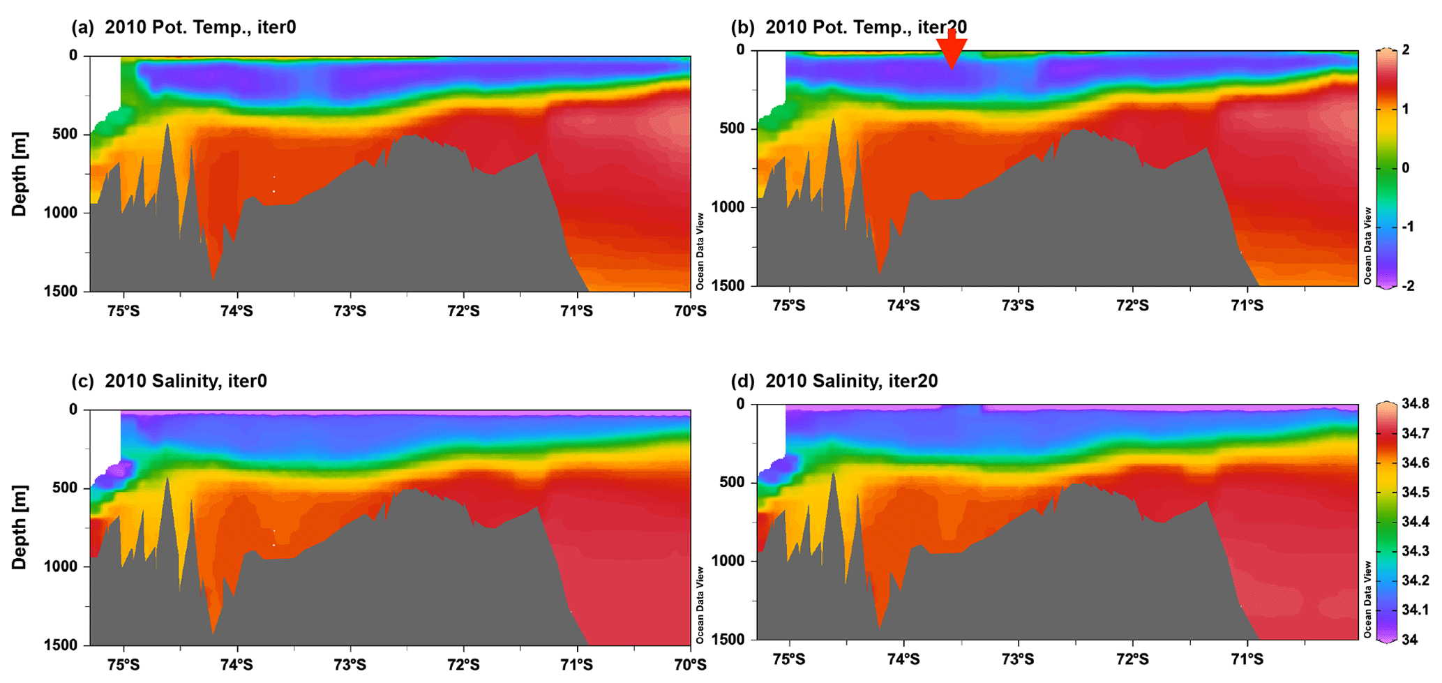
Figure 4 Simulated vertical sections of monthly mean potential temperature (a, b) and salinity (c, d) in January 2010 along the thick black line in Fig. 1 for the (a, c) unoptimized and (b, d) iteration-20 simulations. The red arrow indicates the central part of the AS where thermocline depth is compared.

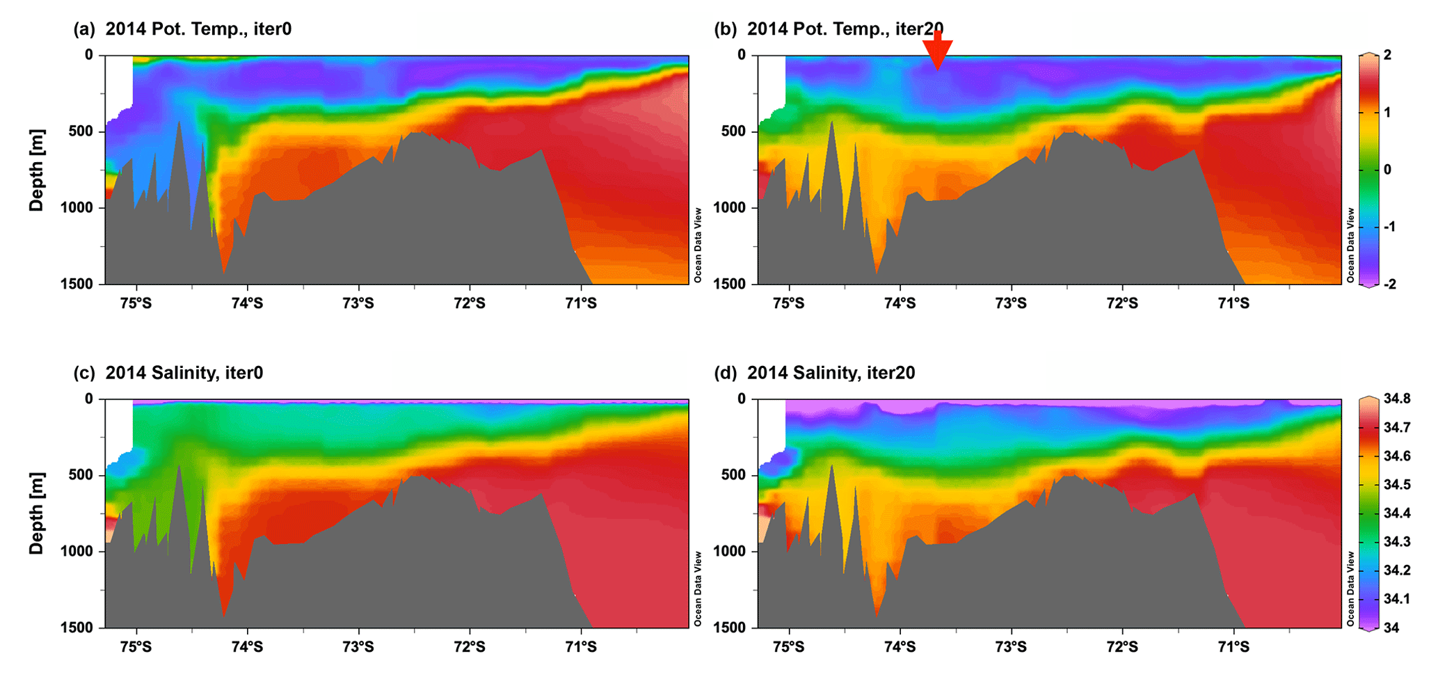
Figure 5 Simulated vertical sections of monthly mean potential temperature (a, b) and salinity (c, d) in January 2014 along the thick black line in Fig. 1 for the (a, c) unoptimized and (b, d) iteration-20 simulations. The red arrow indicates the central part of the AS where thermocline depth is compared.

For the static ice shelf component, the freezing–melting process in the sub-ice-shelf cavity is parameterized by the three-equation thermodynamics of Hellmer and Olbers (1989) and Jenkins (1991). We use constant turbulent heat and salt exchange coefficients for individual ice shelves, which are already adjusted in Nakayama et al. (2017). However, only for Pine Island and Thwaites ice shelves do we further modify these coefficients for simulations after iteration 11 (Table 3), as their ice shelf melt rates become too large. Changes in these coefficients do not highly alter on-shelf circulation (see Fig. S18 in Nakayama et al., 2018), and adjustments of these coefficients in addition to optimizations based on adjoint sensitivities are possible.

3 Results

3.1 Unoptimized simulation (iteration 0)

As we initialize the unoptimized simulation (iteration 0) with simulated oceanographic conditions based on the Green's functions approach (Nakayama et al., 2017), its 2010 simulated vertical section shows a good agreement with observations (Fig. 4). Detailed model–data comparisons are presented for the same section in Nakayama et al. (2017). Simulated vertical sections present mCDW below 400–500 m and WW above 250–400 m, consistent with observations (Fig. 2 in Jacobs et al., 2011, and Fig. 4 in Nakayama et al., 2013). Similarly to Nakayama et al. (2017), slight differences can still be found for WW properties close to the surface (salinity being still too saline (∼0.1 psu)) and PIIS front mCDW properties (∼0.1 psu for salinity and ∼0.2 ^∘C for potential temperature, Fig. 4).

We find, however, that the time evolution of iteration 0 between 2010–2014 does not agree well with observations. For example, oceanographic conditions at the PIIS front in the iteration-0 simulation become too cold and fresh by ∼2 ^∘C and ∼0.25 psu compared to observations, respectively (Figs. 4 and 5). This is clearly different from observations because WW becomes dense, convects to the bottom, and prevents mCDW intrusions into the PIIS cavity in iteration 0 (Fig. 5). Furthermore, the horizontal section of potential temperature at 552 m depth illustrates the formation of cold and fresh water masses (ca. −1 ^∘C and 34.4 psu) in the vicinity of the PIIS (the red arrows in Fig. 6) in contrast to observations (Fig. 3). This water spreads along the coast and induces unrealistic cooling in the large area of the AS (Figs. 6 and 7). Simulated time series of potential temperature and salinity at the PIIS front mooring (Fig. 8) show that these changes occur as a result of intense cooling by the atmosphere in the austral winter of 2013, and this cooling leads to a reduction in the PIIS melt rate by ∼100 Gt yr⁻¹ (Fig. 9a).

3.2 Model–observation differences and improvements

As a result of the iterative optimization, we are able to reduce the cost, which is defined as a sum of the weighted model–data difference, by 65 % by adjusting initial ocean temperature and salinity, atmospheric surface parameters, and vertical diffusivity (Fig. 2). The cost reduction occurs more quickly in the first 10 iterations (Fig. 2). Throughout the optimization, sea-ice and ocean costs are reduced by 59 % and 70 %, respectively.

3.2.1 Sea ice

In the iteration-20 simulation, spatial patterns of sea-ice concentrations show better agreement with observations. For September, the simulated sea-ice area over the entire model domain in iteration 0 is larger than observations by 0.08×10⁶ km² (3.5 % difference), while in iteration 20 it is larger by only 0.03×10⁶ km² (1.2 % difference). September simulated sea-ice concentration is overestimated in iteration 0 at the northern model boundary but becomes much closer to observations in iteration 20 (Fig. 10). For March in the AS, simulated sea ice in iteration 0 is larger than observations by 0.12×10⁶ km² (57 % difference), and in iteration 20 it is larger by 0.08×10⁶ km² (37 % difference). In the BS, simulated sea ice in iteration 0 is larger than observations by 0.13×10⁶ km² (144 % difference), and in iteration 20 it is larger by 0.05×10⁶ km² (56 % difference).

Figure 6 Simulated monthly mean (a, b) potential temperature and (d, e) salinity at 552 m depth in January 2014 for (a, d) unoptimized and (b, e) iteration-20 simulations. (c) Potential temperature and (f) salinity differences between unoptimized and iteration-20 simulations. Bathymetric contours of 500, 2000, and 4000 m are shown in black. Red arrows indicate the PIIS front region, and pink arrows indicate regions in the deep troughs in the AS. In the iteration-20 simulation, potential temperature in these regions becomes warmer as mCDW intrusion into the ice shelf cavities in the AS is correctly represented

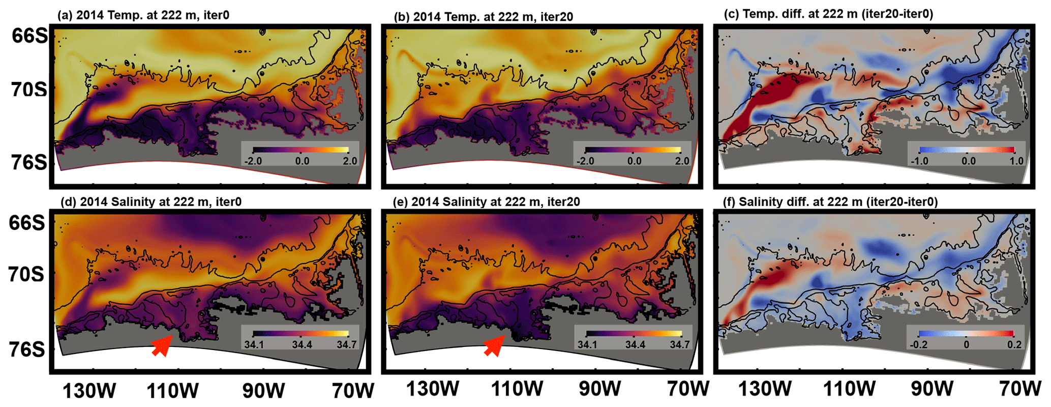
Figure 7 Simulated yearly mean (a, b) potential temperature and (d, e) salinity at 222 m depth in 2014 for (a, d) unoptimized and (b, e) iteration-20 simulations. (c) Potential temperature and (f) salinity differences between unoptimized and iteration-20 simulations. Bathymetric contours of 500, 2000, and 4000 m are shown in black. Red arrows indicate the eastern AS region, where salinity becomes fresher by ∼0.1, showing an improvement in WW properties.

3.2.2 Ocean

For the AS, there are two major improvements for the oceanographic condition: (1) representation of mCDW intrusions towards the ice shelf cavities and (2) properties of WW. For the BS, we do not include enough observational data in the current version of the ocean state estimate and are not able to judge the capability of our state estimation.

As the model–data difference becomes larger towards the end of the 2010–2014 unoptimized simulation, we compare 2014 oceanographic conditions between iteration-0 and iteration-20 simulations to assess improvements. At greater depths, mCDW penetrates along the submarine glacial troughs towards the Pine Island and Thwaites ice shelf cavities (the red arrows in Fig. 6a, b) in the iteration-20 simulation, which is qualitatively similar to observations (Fig. 3b) and other model studies (Jacobs et al., 2011; Nakayama et al., 2013, 2018, 2019; Dutrieux et al., 2014). The 552 m potential temperature and salinity difference between iteration-0 and iteration-20 simulations are ∼0.5 ^∘C and ∼0.1 psu along the coast of the AS, respectively (Fig. 6). Simulated time series of potential temperature and salinity at the PIIS front mooring also show the continuous intrusion of mCDW into the PIIS cavity from 2010–2014, consistent with observations (e.g., Jacobs et al., 2011; Dutrieux et al., 2014; Kim et al., 2017; Jenkins et al., 2018; Assmann et al., 2019).

At shallower depths, the thermocline is located deeper by ∼150 m in the AS in 2014 compared to in 2010 (Figs. 4 and 5), which seems to be consistent with observations (Jacobs et al., 2011; Nakayama et al., 2013; Dutrieux et al., 2014; Heywood et al., 2016). The 222 m salinity difference between iteration-0 and iteration-20 simulations shows freshening by 0.05–0.1 almost everywhere in the AS (the red arrows in Fig. 7d and e). This is a good improvement as WW tends to become too saline in most numerical models (e.g., St-Laurent et al., 2015; Nakayama et al., 2018) and good representations of surface hydrographic conditions as well as of stratification are necessary for the better representation of interannual variabilities.

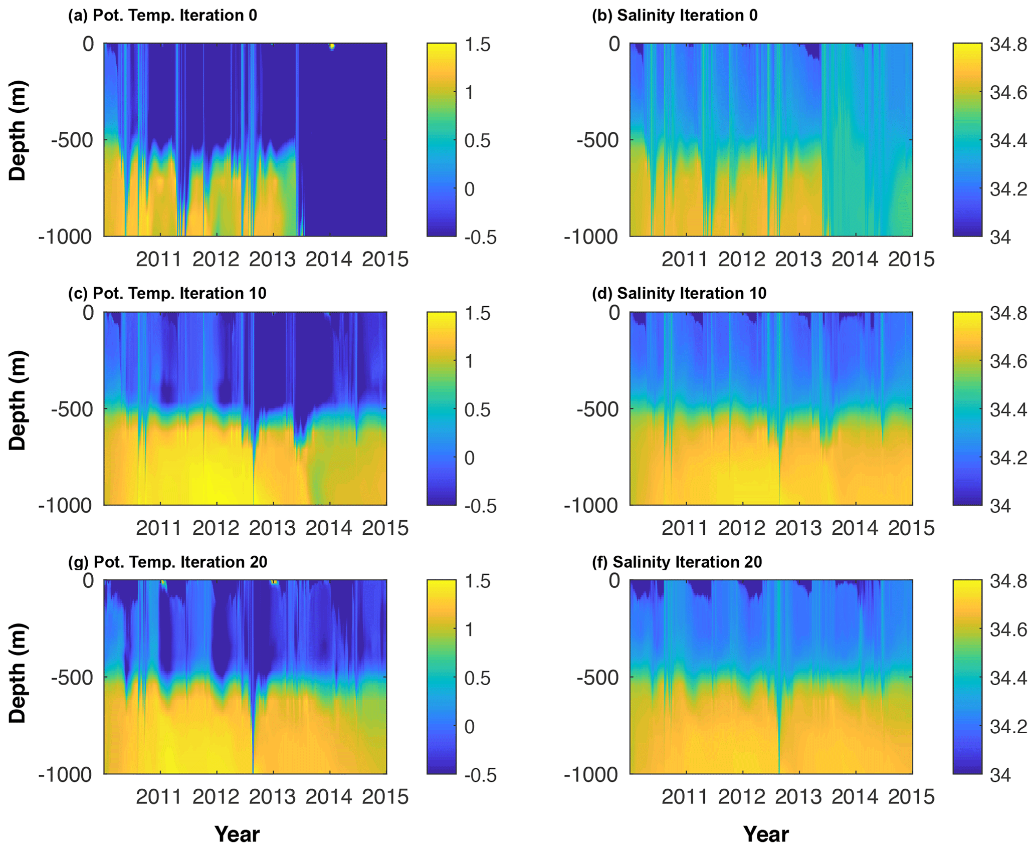
Figure 8 Simulated time series of (a, c, g) potential temperature and (b, d. f) salinity at BSR5 and iSTAR9 mooring locations for (a, b) iteration-0 (unoptimized), (c, d) iteration-10, and (g, f) iteration-20 simulations. Observed mooring time series are shown in Figs. 12 and 2c in Webber et al. (2017).

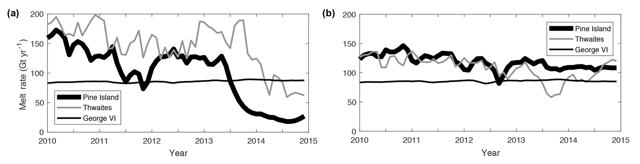
Figure 9 Simulated monthly mean basal melt rates from 2010 to 2015 for the Pine Island, Thwaites, and George Vl ice shelves for (a) unoptimized and (b) iteration-20 simulations.

3.2.3 Ice shelf

Heat and salt transfer coefficients are kept constant, and we do not allow them to change over time for each model iteration. Thus, time series of ice shelf melt rates simply reflect changes in oceanographic conditions in the ice shelf cavities. We note, however, that these coefficients are adjusted once at iteration 11 for Pine Island and Thwaites ice shelves (Tables 3 and 4). In iteration 0, simulated time series of Pine Island and Thwaites ice shelf melt rates show a reduction of ∼100 Gt yr⁻¹ between 2010–2014 (Fig. 9). In the iteration-20 simulation, however, time series of both Pine Island and Thwaites ice shelf melt rates become rather stable at ∼110 Gt yr⁻¹ but show slight decreasing trends of ∼4 and ∼3 Gt yr⁻², respectively. The simulated Pine Island melt rate shows a reduction in 2012 by ∼30 Gt yr⁻¹, and the simulated Thwaites melt rate shows reductions of ∼20 and ∼50 Gt yr⁻¹ in 2012 and 2013, respectively. For ice shelves in the BS, melt rates remain almost constant (e.g., Fig. 9).

(Rignot et al., 2013)

Table 4 Satellite-based estimates of basal melt rate (Rignot et al., 2013) and model mean basal melt rates (2010–2014) for West Antarctic ice shelves for iteration 20. The values of heat transfer coefficient γ_T used for the optimized simulation are also shown. We use constant turbulent heat and salt exchange coefficients for individual ice shelves, which are already adjusted in Nakayama et al. (2017). However, only for Pine Island and Thwaites ice shelves (bold) do we further modify these coefficients for simulations after iteration 11.

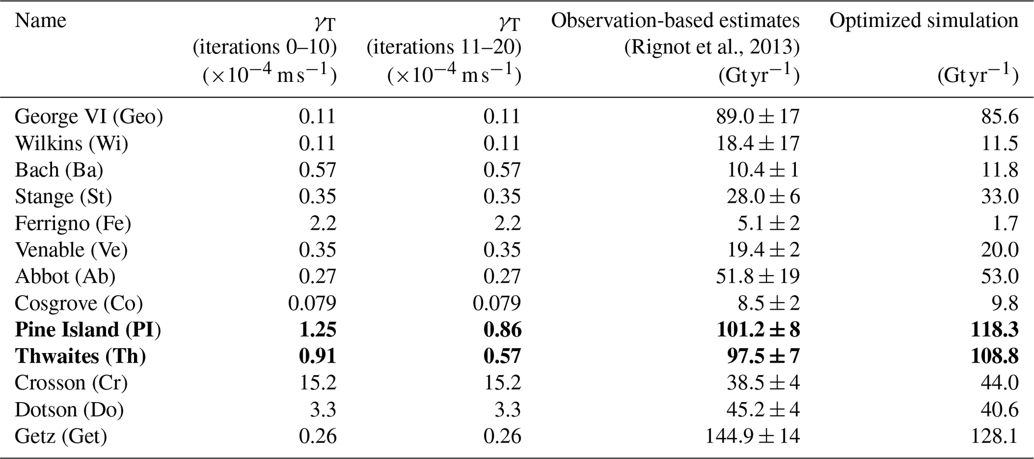
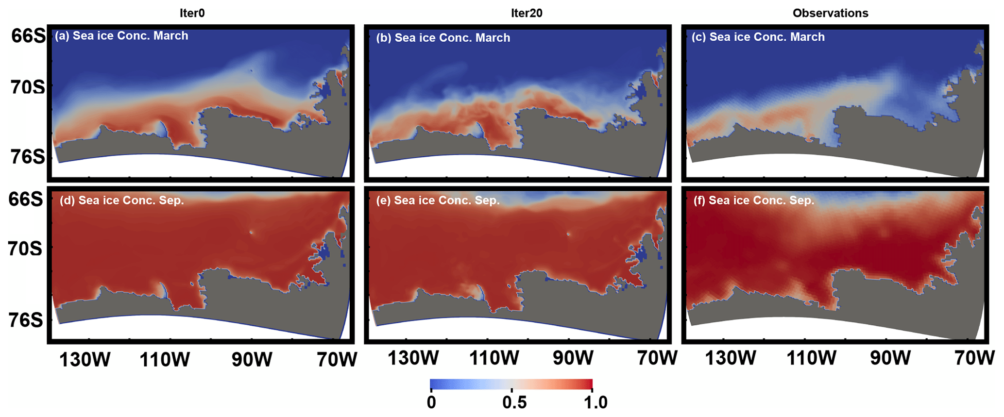
Figure 10 Simulated mean sea-ice concentrations for (a, b) March and (d, e) September for unoptimized and iteration-20 simulations, respectively. The observed mean sea-ice concentrations for (c) March and (f) September based on satellite sea-ice concentration measurements between 2010–2014.

Based on observations, it is suggested that melt rates of Pine Island and Thwaites ice shelves should have decreased between 2012–2014 due to a deepened thermocline (Dutrieux et al., 2014; Webber et al., 2017), and estimated ice shelf melt rates from oceanographic observations are ∼75 and ∼40 Gt yr⁻¹ based on 2009/10 and 2012 observations, respectively. However, these estimates rely on single snapshots of ice shelf front oceanographic observations. Satellite-based estimates of ice shelf melt rates are 101 and 98 Gt yr⁻¹ for Pine Island and Thwaites ice shelves, respectively. These estimates are derived from volume flux divergence of Antarctic ice shelves in 2007 and 2008 with 1979–2010 surface accumulation and 2003–2008 thinning (Rignot et al., 2013) and may represent ice shelf melt rates in warm oceanographic conditions in the eastern AS.

In general, heat and salt transfer coefficients are already adjusted in Nakayama et al. (2017), and melt rates of ice shelves in the AS and BS are consistent with satellite-based estimates (Table 4). The interannual variability in the simulated ice shelf melt rates may be too weakened compared to observations possibly because (1) the coarse horizontal and vertical grids used in this configuration may not allow the realistic representation of ocean cavity circulation and (2) the observed reduction in ice shelf melt rates is caused by changes in ice shelf geometry and it can not be simulated in static ice shelf cavity configurations. Satellite-based estimates of time-evolving ice shelf melt rates are required for further comparison.

Figure 11 (a) Simulated January 2014 mean 552 m potential temperature for iteration 20. Simulated potential temperature differences of (b) NoWindAdj, (c) NoPrepAdj, and (d) NoAtempAdj compared to the iteration-20 simulation. Bathymetric contours of 500 and 2000 m are shown in black. Spatial averages of 552 m potential temperature are calculated for the region enclosed by the red boxes.

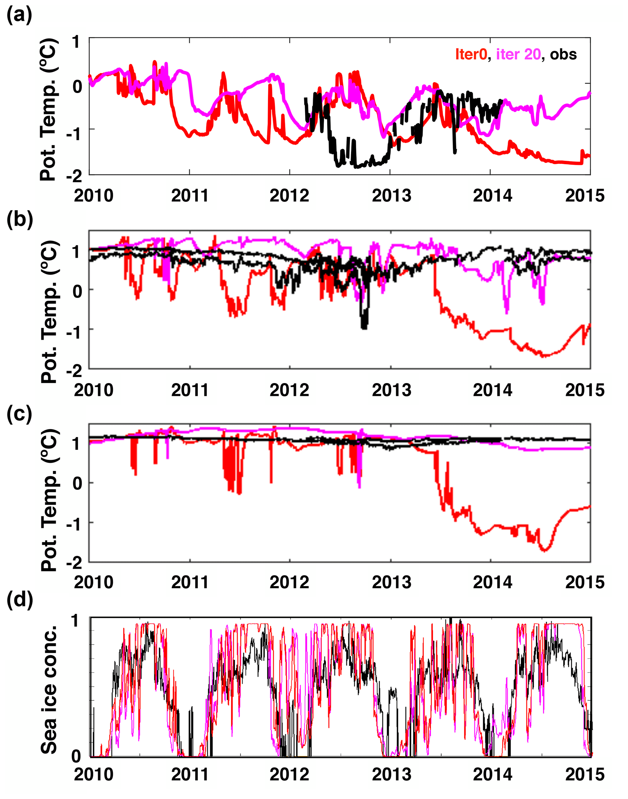
Figure 12 Time series of simulated potential temperature at (a) 409 m, (b) 34 m, and (c) 909 m for unoptimized (iteration 0) and iteration-20 simulations. Time series of observed potential temperature at BSR5 and iSTAR9 mooring sites at depths of approximately (a) 400 m; (b) 600, 650, 700 m; and (c) 780 and 900 m are also shown in black. Time series of (d) spatially averaged (74.8–75.0^∘ S, 102.4–104.0^∘ W) sea-ice concentration for the unoptimized simulation (iteration 0), iteration 20, and observations.

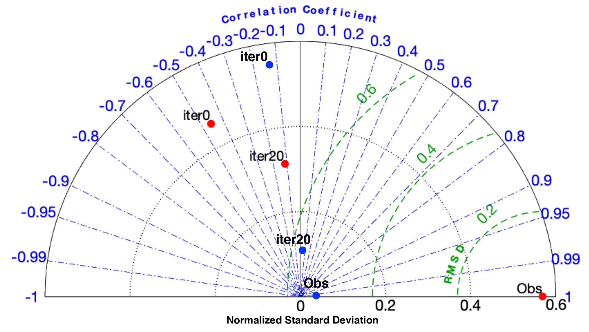
Figure 13 Taylor diagram listing the statistical properties of 400 m (red) and 900 m (blue) potential temperature at PIIS front from mooring observations and simulations from iterations 0 and 20. The radial distances from the center of the semi-circle represent the standard deviation of each time series. The angle represents the correlation coefficient between the observed and simulated daily time series of potential temperature. The dashed green curves centered on the “Obs” point are a scale for the root mean square differences (between the observed time series and each simulated time series). The Taylor diagram was drawn using the MATLAB routine TAYLORDIAG developed by Guillaume Maze.

Table 5 Description of all the sensitivity simulations.

4 Discussion

4.1 Sensitivity studies

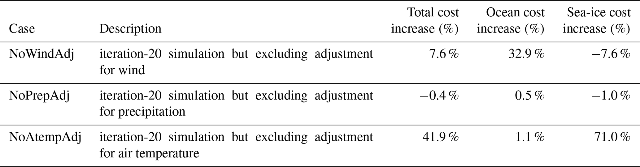
To investigate the reason for the improvements, we conducted three sensitivity experiments (Table 5) as air temperature, precipitation, and wind are considered the main drivers of oceanographic variabilities at the PIIS front region. For the NoWindAdj, NoPrepAdj, and NoAtempAdj cases, we re-ran the iteration-20 simulation but excluded adjustments for wind, precipitation, and air temperature, respectively. The total costs are 2.9×10⁶, 3.1×10⁶, 2.9×10⁶, and 4.1×10⁶ for the iteration-20, NoWindAdj, NoPrepAdj, and NoAtempAdj cases, respectively, showing that adjustments of wind and atmospheric temperature play important roles in reducing both sea-ice and ocean costs. Sea-ice costs are 1.7×10⁶, 1.6×10⁶, 1.7×10⁶, and 2.9×10⁶ for the iteration-20, NoWindAdj, NoPrepAdj, and NoAtempAdj cases, respectively. Ocean costs are 1.1×10⁶, 1.5×10⁶, 1.1×10⁶, and 1.2×10⁶ for the iteration-20, NoWindAdj, NoPrepAdj, and NoAtempAdj cases, respectively. Cost function increases in these sensitivity experiments compared to the control are summarized in Table 5, showing that adjustment of wind has the strongest impact on the ocean, while adjustment of air temperature has the strongest impact on sea ice.

Among these sensitivity experiments, the January 2014 mean potential temperature at 552 m depth shows a similar spatial pattern for all cases for open ocean and in the BS (not shown), and differences can only be found in the AS especially at the PIIS front (Fig. 11). Spatially averaged 552 m potential temperatures at the PIIS front (averaged for the region enclosed by the red box in Fig. 11a) are 0.61, 0.23, 0.56, and 0.53 ^∘C for the iteration-20, NoWindAdj, NoPrepAdj, and NoAtempAdj cases, respectively. Vertically integrated heat contents, which are strongly controlled by thermocline depth (Nakayama et al., 2018), reduced by 11 %, 5 %, and 12 % for the NoWindAdj, NoPrepAdj, and NoAtemAdj cases, respectively, compared to the iteration-20 solution. This implies that (1) PIIS front mCDW temperature and thus mCDW pathways as well as strength of intrusions are dominantly controlled by wind and (2) the PIIS front thermocline depth is influenced rather equally by wind, precipitation, and air temperature.

4.2 Seasonal and interannual variability

Mooring observations at the PIIS front were conducted from 2009–2014, which provide us with potential temperature measurements at various depths (Webber et al., 2017). At depths below 800 m, the observed potential temperature remains rather stable at ∼1 ^∘C (Fig. 12c). At 600–700 m depths, the potential temperature also remains stable at 1 ^∘C and shows gradual cooling and warming between 2010–2012 and 2013–2015, respectively (Fig. 12). Between 2012–2013, however, the potential temperature time series shows sporadic emergence of cold water masses (ca. −0.5 ^∘C). At 400–500 m depths, the time series of potential temperature fluctuates between −1.8 ^∘C and 0 ^∘C and seasonal and interannual variabilities are large.

For iteration 0, we find three major differences with respect to the observations (Fig. 12); (1) simulated potential temperature shows rapid cooling between 2013–2015 and potential temperature at all depths changes from ca. 1 ^∘C to ca. −1 ^∘C; (2) simulated time series of potential temperature shows sudden emergence of cold water at all depths throughout the simulated period, while it occurs only for shallower depths for observations; and (3) the timing of cooling and warming does not agree with observations. These sporadic coolings are likely associated with strong wind events which lead to the formation of cold and dense water and deep convection.

For the iteration-20 simulation, simulated time series show improvements at all depths (Fig. 12). At greater depths (800–900 m), the potential temperature remains rather stable at ∼1 ^∘C, consistent with observations (Fig. 12c), and the sudden emergence of cold water only occurs at shallower depths. However, the long-term and short-term variabilities have large differences between observations and the iteration-20 simulation, and the timings of cooling and warming still do not agree with observations. Such differences are also presented in Taylor diagrams based on simulated and observed time series of 400 and 900 m potential temperature at the PIIS front (Fig. 13). The root mean square differences reduce by 23 % and 80 % for iterations 0 and 20, respectively. However, standard deviations and correlation coefficients of both the iteration-0 and the iteration-20 solutions retain large differences compared to observations. This means that current states of the optimized solution achieve better agreement in terms of mean states, but it remains difficult to capture shorter timescale variability for both time series at the middle and close to the bottom of the water column.

One possible reason for the difference is deficiencies in the simulated sea-ice concentration near the coast. In our current configuration using a pseudo-sea-ice adjoint sensitivity, we are not able to directly adjust sea-ice concentration: simulated sea-ice concentration at the PIIS front remains almost the same between the iteration-0 and iteration-20 simulations (Fig. 12). More accurate representations of sea ice would likely allow us to capture, for example, wind-driven transports of sea ice away from the coast, surface ocean cooling, and sea-ice formation. Such processes likely change the local stratification, which possibly impacts warm mCDW intrusions into the PIIS cavity.

5 Conclusions

In previous work, Nakayama et al. (2017) employed a Green's functions approach to adjust a numerical simulation of 2010 AS conditions close to observations. However, we find that continuation of the Nakayama et al. (2017) setup until the year 2014 leads to unrealistic cooling and freshening at the PIIS front and other coastal regions of the AS (Figs. 4–6, 8).

In this work, we develop an Amundsen Sea–Bellingshausen Sea ocean simulation following Nakayama et al. (2017) and employ the ECCO ocean state estimation tools based on adjoint sensitivities (Forget et al., 2015; Zhang et al., 2018) to develop an ocean state estimate for the AS and BS for the time period of 2010–2014. We choose this time window because the largest interannual variability was observed after the first observations in 1994 (Dutrieux et al., 2014) and a good number of oceanographic observations are available. After 20 iterations, the cost function, which is defined as a sum of the weighted model–data difference, is reduced by 65 % by adjusting initial conditions, atmospheric forcing, and vertical diffusivity (Fig. 2). The iteration-20 simulation can simulate oceanographic conditions much closer to observations for the 2010–2014 period compared to the unoptimized iteration-0 simulation. The main improvements are (1) simulated sea-ice extent for the AS and BS, (2) simulated WW properties and thermocline depths in the AS (Fig. 12), and (3) simulated mCDW intrusions towards AS ice shelf cavities and their pathways (Figs. 5–7). Despite the improvements listed above, the seasonal and interannual variability in oceanographic conditions at the PIIS front is not simulated well compared to the mooring observations and it remains difficult to simulate seasonal and interannual changes in oceanographic conditions on the AS continental shelf (Fig. 12).

There are several lines of investigation that can improve upon the technical foundation discussed hereinabove. This includes new sea-ice adjoint optimization code (Fenty and Heimbach, 2013a; Bigdeli et al., 2020), improved methods of calculating costs to put more emphasis on the seasonal and interannual variabilities (Forget et al., 2015), adding other oceanographic datasets not used in the current optimization such as additional mooring observations (Assmann et al., 2019) and instrumented pinnipeds (Roquet et al., 2013), more careful estimation of model and data prior uncertainty, and a number of new optimizations from different initial conditions and parameter guesses to ensure the robustness of the optimized solution. Considering the grid resolution selected for this regional model (10 km horizontal grid spacing), this work is a step towards the improved representation of ice shelf–ocean interaction in the ECCO (Estimating the Circulation and Climate of the Ocean) global ocean retrospective analysis as well as in current-generation IPCC (Intergovernmental Panel on Climate Change) global climate models.