the Creative Commons Attribution 4.0 License.
the Creative Commons Attribution 4.0 License.
 | 29 Jul 2021
DecTree v1.0 – chemistry speedup in reactive transport simulations: purely data-driven and physics-based surrogates
Michael Kühn
The computational costs associated with coupled reactive transport
simulations are mostly due to the chemical subsystem: replacing it
with a pre-trained statistical surrogate is a promising strategy to
achieve decisive speedups at the price of small accuracy losses and
thus to extend the scale of problems which can be handled. We
introduce a hierarchical coupling scheme in which “full-physics”
equation-based geochemical simulations are partially replaced by
surrogates. Errors in mass balance resulting from multivariate
surrogate predictions effectively assess the accuracy of
multivariate regressions at runtime: inaccurate surrogate
predictions are rejected and the more expensive equation-based
simulations are run instead. Gradient boosting regressors such as
XGBoost, not requiring data standardization and being able to handle
Tweedie distributions, proved to be a suitable emulator. Finally, we
devise a surrogate approach based on geochemical knowledge, which
overcomes the issue of robustness when encountering previously
unseen data and which can serve as a basis for further development of
hybrid physics–AI modelling.
- Article
(3710 KB) - Full-text XML
- BibTeX
- EndNote


Coupled reactive transport simulations (Steefel et al., 2005, 2015) are very expensive, effectively hampering their wide applications. While hydrodynamic simulations on finely resolved spatial discretizations, containing millions of grid elements, are routinely run on common workstations, the order of magnitude of the computationally affordable reactive transport simulations on the same hardware decreases by a factor of 10 to 100 as soon as chemical reactions are coupled in (De Lucia et al., 2015; Jatnieks et al., 2016; Laloy and Jacques, 2019; Leal et al., 2020; Prasianakis et al., 2020). This usually requires oversimplifications of the subsurface domain, reduced to 2D or very coarse 3D, and of the geochemical complexity as well.
In classical operator splitting such as the sequential non-iterative approach (SNIA), the three interacting physical processes of hydrodynamic flow, solute transport, and chemical interactions between solute species and rock-forming minerals are solved sequentially. Chemistry usually represents the bottleneck for coupled simulations, taking up between 90 % and 99 % of compute time (Steefel et al., 2015; He et al., 2015; De Lucia et al., 2015; Huang et al., 2018; Leal et al., 2020). The numerical model for geochemical speciation and reactions generally requires the integration of one stiff differential–algebraic system of equations per grid element per simulation time step. Parallelization is thus required to tackle large spatial discretizations, which is why many modern codes are developed to run on high-performance computing (HPC) clusters with many thousands of CPUs (Hammond et al., 2014; Beisman et al., 2015; Steefel, 2019). However, the problem of difficult numerical convergence for the geochemical subprocess routinely encountered by many practitioners is not solved by parallelization. Furthermore, large uncertainties affect the phenomenological model itself. Kinetics rates in natural media span over orders of magnitude (Marty et al., 2015); activity models for the brines usually encountered in the subsurface lack parameterization for higher temperature, salinity, or for many elements (Dethlefsen et al., 2011; Appelo et al., 2013; Moog et al., 2015); and even larger uncertainty concerns the parameterization of the subsurface, regarding, for example, the heterogeneity of rock mineralogy, which is mostly unknown and hence often disregarded (De Lucia et al., 2011; Nissan and Berkowitz, 2019). It may thus appear unjustified to allocate large computational resources to solve very expensive yet still actually oversimplified or uncertain problems. Removing the computational cost associated with reactive transport modelling is thus of paramount importance to ensure its wide application to a range of otherwise practically unfeasible problems (Prommer et al., 2019).
The much desired speedup of this class of numerical models has been the focus of intensive research in the last few years. Among the proposed solutions, Jatnieks et al. (2016) suggest replacing the full-physics numerical models of the geochemical subsystem with emulators or surrogates employed at runtime during the coupled simulations. A surrogate in this sense is a statistical multivariate regressor which has to be trained in advance on a set of pre-calculated full-physics solutions of the geochemical model at hand, spanning the whole parameter range expected for the simulations. Since the regressors are much quicker to compute than the setup and integration of a differential–algebraic system of equations (DAE), this promises a significant speedup and has thus found resonance in the scientific community (e.g. De Lucia et al., 2017; Laloy and Jacques, 2019; Guérillot and Bruyelle, 2020). However, all approximations and especially purely data-driven surrogates introduce accuracy losses into the coupled simulations. These must be kept low in order to generate meaningful simulation results. Ultimately, replacing a fully fledged geochemical simulator with a surrogate equals trading computational time for accuracy of the simulations. Due to the non-linear nature of geochemical subprocesses, even small errors in surrogate predictions propagate in successive iterations so that diverging trajectories for the coupled models originate from only a few time steps, leading to unphysical results. Mass and charge imbalances, i.e. “creation” of matter, happen to be the most common source of unphysicality in our early tests. It is thus of paramount importance to obtain highly accurate surrogates, which in turn may require very large and densely sampled training datasets and training times.
The thriving developments in data science and machine learning in recent years have produced many different and efficiently implemented regressors readily available and usable in high-level programming languages such as Python or R. Among the most known ones are Gaussian processes, support vector machines, artificial neural networks, and decision-tree-based algorithms such as random forest or gradient boosting. Most of these algorithms are “black boxes”, which non-linearly relate many output variables to many input variables. Their overall accuracy can be statistically assessed by measuring their performances on the training dataset or on a subset of the available training data left out for the specific purpose of testing the models. In any case these training and/or test datasets must be obtained beforehand by computing an appropriate number of points with the full-physics model. Geochemistry is usually largely multivariate, meaning that many input and many output variables are passed to and from the geochemical subsystem at each time step. In general, different regressors may capture each output variable in better fashion depending on many factors (e.g. the problem at hand, in which variables display different non-linear behaviours; the sampling density of the training dataset, which may be biased). With algorithms such as artificial neural networks (ANNs) it is possible to train one single network and hence in practice one single surrogate model for all output variables at once. While ANNs in particular usually require long CPU times for training and quite large training datasets, they offer large speedups when used for predictions (Jatnieks et al., 2016; Prasianakis et al., 2020), and furthermore they can efficiently leverage GPUs (graphic processing units) for even larger acceleration. It is, however, difficult to achieve the required accuracy simultaneously for all output variables (Kelp et al., 2020). For this reason, we focus on a more flexible approach of multiple multivariate regression: one distinct multivariate regressor – i.e. making use of many or all inputs as predictors – is trained independently for each distinct output variable. This approach allows using different specialized models from variable to variable, including different regression methods altogether, but also data preprocessing and hyperparameter tuning, while not necessarily requiring larger computing resources.
This work showcases and analyses two different approaches for surrogate geochemical modelling in reactive transport simulations. The first is completely data-driven, disregarding any possible knowledge about the ongoing process. In the second approach, we derive a surrogate which exploits the actual equations solved by the full-physics representation of chemistry. Both are applied and evaluated on the same 1D benchmark implemented in a simple reactive transport framework. Our implementation of coupled reactive transport includes a hierarchical submodel coupling strategy, which is advantageous when different accuracy levels for the predictions of one subprocess are available.
The versioned R code used for DecTree v.1.0 model setup and evaluation
is referenced in the section “Code availability”. It is based on version
v0.0.4 of the RedModRphree package for the R environment
(R Core Team, 2020), which is also referenced in the section “Code
availability”. It makes use of the geochemical simulator PHREEQC
(Appelo et al., 2013). RedModRphree supersedes the in-house-developed R-PHREEQC interface Rphree
(https://rphree.r-forge.r-project.org/, last access: 23 July 2021, De Lucia and Kühn, 2013).
The benchmarks and the performance measurements refer to computations run on a recent desktop workstation equipped with an Intel Xeon W-2133 CPU with clock at 3.60 GHz and DDR4 RAM at 2.666 GHz under Linux kernel 5.9.14 and R version 4.0.3. If not otherwise specified, only one CPU core is employed for all computational tasks. Since in an operator-splitting approach the simulation of geochemical subprocess is inherently an embarrassing parallel task, in which at each time step one geochemical simulation per grid element is required completely independent of the neighbours, the speedup achieved on a single CPU as in this work will transfer on parallel computations in which each CPU is assigned a comparable number of grid elements up to the overhead required to dispatch and collect the results in a parallel environment.
2.1 Numerical simulation of flow and transport
We consider a stationary, fully saturated, incompressible, isothermal 1D Darcy flow in a homogeneous medium. Transport is restricted to pure advection, and the feedback of mineral precipitation and dissolution on porosity and permeability is also disregarded; the fluid density is considered constant. Advection is numerically computed via a forward Euler explicit resolution scheme:
where u is the module of Darcy velocity, Ci(x,t) the volumetric concentration (molality) of the ith solute species at point x and time t, and Δ x the size of a grid element. For this scheme, the Courant–Friedrichs–Lewy stability condition (CFL) imposes that the Courant number ν be less than or equal to 1:
For Courant numbers less than 1, numerical dispersion arises; the scheme is unstable for ν>1. The only both stable and precise solution for advection is with ν=1. Thus, the CFL condition is very limiting in Δ t: a factor of 2 refinement in the spatial discretization corresponds to a factor of 2 decrease in Δ t, thus requiring twice the coupling iterations. Note that porosity is not considered in Eq. (1) so that effectively the Darcy velocity is to be assumed equal to the seepage velocity or, alternatively, porosity is equal to unity. This assumption does not have any impact on the calculations beside the volumetric scaling that has to be considered for the minerals. In the code the mineral amounts are always treated as moles per kilogramme of solvent.
The implemented advection relies on transport of total elemental concentrations instead of the actual dissolved species, an allowable simplification since all solutes are subjected to the same advection equation (Parkhurst and Wissmeier, 2015). Total dissolved O, H, and solution charge should be included among the state variables and thus transported, but since this problem is redox-insensitive, we can disregard charge imbalance and only transport pH instead of H and O, disregarding changes in water mass. The pH is defined in terms of activity of protons,
and is hence not additive. If we further assume that the activity coefficient of protons stays constant throughout the simulation, the activity [H+] can actually be transported. The resulting simplified advective model shows negligible deviations from the results of the same problem simulated with PHREEQC's ADVECTION keyword (not shown).
2.2 The chemical benchmark
The chemical benchmark used throughout this work is inspired by Engesgaard and Kipp (1992) and is well known, with many variants, in the reactive transport community (e.g. Shao et al., 2009; Leal et al., 2020). It was chosen since it has been studied by many different authors and is challenging enough from a computational point of view.
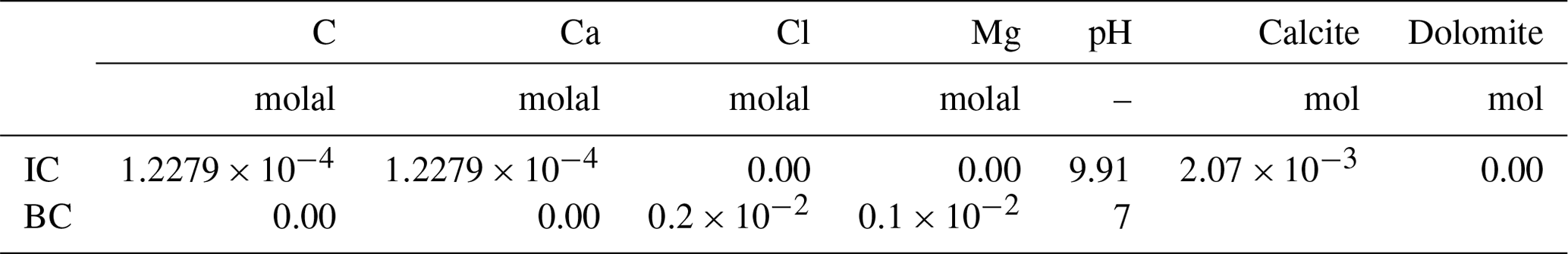
At the inlet of a column, conventionally on the left side in the pictures throughout this work, a 0.001 molal magnesium chloride (MgCl2) solution is injected into a porous medium whose initial solution is at thermodynamic equilibrium with calcite. With the movement of the reactive front, calcite starts to dissolve and dolomite is transiently precipitated. Kinetic control is imposed on all mineral reactions following a Lasaga rate expression from Palandri and Kharaka (2004), which is limited to only neutral and H+ mechanisms (parameters are summarized in Table 1) and constant reactive surfaces; hence, it is independent of the actual amounts of minerals. Precipitation rate – relevant only for dolomite – is set equal to the rate of dissolution. Temperature is set for simplicity at a constant 25 ∘C in disregard to actual physical meaningfulness of the model concerning dolomite precipitation (Möller and De Lucia, 2020). Detailed initial and boundary conditions are summarized in Table 2.
Table 1Parameters for kinetic control for dissolution and precipitation of calcite and dolomite. k is given in mol m−2 s−1, Ea in kJ mol−1, and reactive surface in m2 kg.
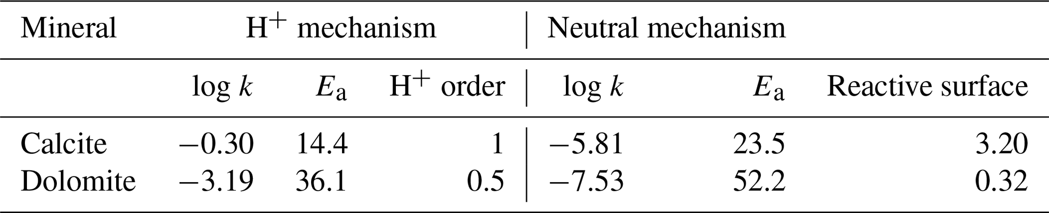
Table 2Initial conditions (ICs) and boundary conditions (BCs) for the benchmark problem.
To achieve a complete description of the chemical system at any time, seven input variables are required: pH, C, Ca, Mg, Cl, calcite, and dolomite – those can be considered state variables, since they constitute the necessary and sufficient inputs of the geochemical subsystem, and all reactions only depend on them. The outcome of the full-physics calculations is completely defined (at least with the simplifications discussed above) by four distinct quantities: the amounts of reaction affecting the two minerals calcite (i) and dolomite (ii) in the given time step, from which the changes in solutes Ca, Mg, and C can be back-calculated; Cl (iii), which is actually non-reactive; and pH (iv). In a completely process-agnostic, data-driven framework, however, the relationships between minerals and aqueous concentrations are disregarded, and the output of the chemical subsystem is expressed solely in terms of the input variables.
2.3 Reference simulations and training data
For the remainder of this work, the geochemical benchmark described above is solved on a 1D column of length 0.5 m, with a constant fluid velocity of m s−1. The domain is discretized with grid refinements ranging between 50 and 500 grid elements. Higher refinements have a double effect: on one side larger grids obviously increase the overall computational load, in particular for chemistry; on the other side, given the restriction of the implemented forward Euler explicit advection scheme, the time stepping required for the coupled simulations in order to be free of numerical dispersion decreases accordingly. Smaller time steps decrease the computational load for geochemistry for each iteration, since they require shorter time integrations, but they also require more coupled iterations to reach the same simulation time. More iterations also mean that there are more chances for errors introduced by surrogates to further propagate into the simulations in both space and time. In the presence of significant overhead due to e.g. data passing between different software or the setup of geochemical simulations, the advantage due to shorter time steps vanishes. However, these aspects become more relevant in the context of parallelization of geochemistry and are not addressed in the present work.
All coupled simulations, both reference (full physics) and with surrogates, are run with a constant time step either honouring the CFL condition with ν=1, and thus free of numerical dispersion, or, when assessing how the speedup scales with larger grids, a fixed time step small enough for the CFL condition (Eq. 2) to be satisfied for every discretization. As previously noted, the resulting simulations will be affected by grid-dependent numerical dispersion, which we do not account for in the present work. This makes the results incomparable in terms of transport across grids. However, since the focus is on the acceleration of geochemistry through pre-computed surrogates, this is an acceptable simplification.
The comparison between the reference simulations obtained by coupling of transport with the PHREEQC simulator and those obtained with surrogates is based on an error measure composed as the geometric mean of the relative root mean square errors (RMSEs) of each variable i using the variable's maximum at a given time step as a norm:
where m is the number of variables to compare, n the grid dimension, and t the particular time step in which the error is computed.
In this work the datasets used for training the surrogates are obtained directly by storing all calls to the full-physics simulator and its responses in the reference coupled reactive transport simulations, possibly limited to a given simulation time. This way of proceeding is considered more practical than e.g. an a priori sampling of a given parameter space; the bounds of the parameter space are defined by the ranges of the input/output variables occurring in the reference coupled simulations. This strategy mimics the problem of wanting to train surrogates directly at runtime during the coupled simulations. Furthermore, an a priori statistical sampling of parameter space, in the absence of restrictions based on the physical relationships between the variables, would include unphysical and irrelevant input combinations. By employing only the input/outputs tables actually required by the full-physics simulations, this issue is automatically solved; however, the resulting datasets will be generally skewed, multimodal, and highly inhomogeneously distributed within the parameter space, with highly dense samples in some regions and even larger empty ones.
2.4 Hierarchical coupling of chemistry
In this work we consider only a sequential non-iterative approach (SNIA) coupling scheme, meaning that the subprocess flow, transport, and chemistry are solved numerically one after another before advancing to the next simulation step. For the sake of simplicity, we let the CFL condition (2) for advection dictate the allowable time step for the coupled simulations.
Replacing the time-consuming, equation-based numerical simulator for geochemistry with an approximated but quick surrogate introduces inaccuracies into the coupled simulations. These may quickly propagate in space and time during the coupled simulations and lead to ultimately incongruent and unusable results.
A way to mitigate error propagation, and thus to reduce the accuracy required of the surrogates, is represented by a hierarchy of models used to compute chemistry at each time step during the coupled simulations. The idea is to first ask the surrogate for predictions, then identify implausible or unphysical ones, and finally run the full-physics chemical simulator for the rejected ones. This way, the surrogate can be tuned to capture the bulk of the training data with good accuracy, and no particular attention needs to be paid to the most difficult “corner cases”. For the highly non-linear systems usually encountered in geochemistry, this is of great advantage. In practice, however, there is still a need to have a reliable and cheap error estimation of surrogate predictions at runtime.
It is important to understand that the criteria employed to accept or reject the surrogate predictions depend strictly on the architecture of the multivariate surrogate and on the actual regression method used. Methods such as kriging offer error variances based on the distance of the target estimation point from the data used for estimation for a given variogram model. However, in the general case, any error estimation first requires the training and then the evaluation at runtime of a second “hidden” model. Both steps can be time-consuming; furthermore, in the general case one can only guarantee that the error is expected – in a probabilistic sense – to be lower than a given threshold.
In a completely data-driven surrogate approach whereby each of the output variables is independently approximated by a different multivariate regressor, checking mass conservation is a very inexpensive way to estimate the reliability of a given surrogate prediction, since it only requires the evaluation of linear combinations across predictors and predictions. Other constraints may be added that are suited to the chemical problem at hand, such as charge balance. However, we only use mass balance in the present work. Figure 1 illustrates this simple hierarchical coupling schematically.
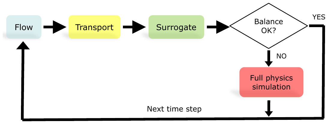
Figure 1Schematic view of hierarchical sequential non-iterative coupling. The decision on whether or not to accept the predictions of a multiple multivariate surrogate is based on computing the mass balances for the three elements forming dolomite and calcite before and after reaction and computing their mean absolute error. If this error exceeds a given threshold, the more expensive equation-based geochemical simulator is run instead.
For the chemical benchmark of Sect. 2.2, three mass balance equations can be written, one for each element C, Ca, and Mg, accounting for the stoichiometry of the minerals' brute formulas. If a surrogate prediction exceeds a given predetermined tolerance on the mean absolute error of the balance equations, that particular prediction is rejected and a more expensive full-physics simulation is run instead.
This approach moderates the need for extremely accurate regressions, especially in instances of non-linear behaviour of the chemical models, for example when a mineral precipitates for the first time or when it is completely depleted, which are hard things for regressors to capture. However, the number of rejected simulations must be low to produce relevant speedups; it is effectively a trade-off between the accuracy of the surrogates (and the effort and time which go into it) and the speedup achieved in coupled simulations.
The first approach is a completely general one that is fully data-driven and thus process-agnostic: it can be employed for any kind of numerical model or process which can be expressed in the form of input and output tables. In our case, the tables produced by the geochemical subprocess during the reference coupled simulations are used to train seven multiple multivariate regressors, one for each output.
The reference simulations, and hence the dataset for training the surrogate, are fully coupled simulations on grids 50, 100, and 200 with a fixed time step of 210 s run until 33 600 s or else 161 total coupling iterations. The time step is chosen to result in ν=1 in the largest grid. As previously noted, these simulations are then not comparable among themselves due to the introduction of numerical dispersion in the lower-resolution grids; however, from the point of view of geochemical processes, this strategy has the advantage of spreading the sampling of the parameter space for the chemical subprocess, while eliminating the time step as a free variable. In this setting, one single trained surrogate can be employed on all grids and time steps.
Instead of the usual random split of the dataset into training and testing subsets, which is customary in the machine-learning community, we retained only the data resulting from the first 101 iterations for training the surrogates and evaluated the resulting reactive transport simulations until iteration 161, during which the geochemical surrogate is faced with 60 iterations on unseen or “out-of-sample” geochemical data. The training dataset comprises tables with 13 959 unique rows or input combinations. All simulations, including the reference and those with surrogates, are run on a single CPU core. No further filtering, i.e. elimination of data points very near each other, has been performed. The data do not display clear collinearity, which is expected with geochemistry being a non-linear process.
The choice of the regressor for each output is actually arbitrary, and nothing forbids having different regressors for each variables or even different regressors in different regions of parameter space of each variable. Without going into detail on all the kinds of algorithms that we tested, we found that decision-tree-based methods such as random forest and their recent gradient boosting evolutions appear to be the most flexible and successful for our purposes. Their edge can in our opinion be resumed by (1) implicit feature selection by construction, meaning that the algorithm automatically recognizes which input variables are most important for the estimation of the output. Note that colinearity is usually not an issue for geochemical simulations; (2) there is no need for standardization (e.g. centring, scaling) of inputs and outputs, which helps preserve the physical meaning of variables. (3) They are fairly quick to train with sensible hyperparameter defaults, although they are slower to evaluate than neural networks. (4) There is robustness, since they revert to mean value when evaluating points outside of training data.
Points (2)–(4) cannot be overlooked. Data normalization or standardization techniques, also called “preprocessing” in machine-learning lingo, are redundant with decision-tree-based algorithms, whereas they have a significant impact on results and training efficiency with other regressors such as support vector machines and artificial neural networks. The distributions displayed by the variables in the geochemical data are extremely variable and cannot be assumed to be uniform, Gaussian, or lognormal in general. We found that the Tweedie distribution is suited to reproduce many of the variables in the training dataset. The Tweedie distribution is a special case of exponential dispersion models introduced by Tweedie (1984) and thoroughly described by Jørgensen (1987), which finds application in many actuarial and signal processing processes (Hassine et al., 2017). A random variable Y is a Tweedie distribution of parameter p if Y≥0, E[Y]=μ and Var(Y)=σ2 μp. This means that it is a family depending on p: Gaussian if p=0, Poisson if p=1, gamma if p=2, and inverse Gaussian if p=3. The interesting case, which is normally referred to when using the term “Tweedie”, is when . This distribution represents positive variables with positive mass at zero, meaning that this distribution preserves the “physical meaning” of zero. It is intuitively an important property when modelling solute concentrations and mineral abundances: the geochemical system solved by the full-physics simulator is radically different when e.g. a mineral is present or not.
Extreme gradient boosting or XGBoost (Chen and Guestrin, 2016) is a
decision-tree-based algorithm which has enjoyed enormous success in the
machine-learning community in recent years. Out of the box, it has the
capability to perform regression of Tweedie variables and is
extremely efficient in both training and prediction. The package has
support for GPU computing but we did not use it in the present work.
Using the target Tweedie regression with fixed p=1.2, max tree depth
of 20, the default η=0.3, and 1000 boosting iterations with
early stopping at 50, all results in the dataset are reproduced with
great accuracy and the training itself takes around 20 s for all
seven outputs on our workstation using four CPU cores. Contrary to
the expectation and specific statements in the software package, we
found that scaling – not re-centring – the labels by their maximum
value divided by , thus spreading the range of the
scaled outputs from 0 to 105, greatly improves the
accuracy. We did not pursue a more in-depth analysis of this issue,
since it probably depends on this specific software, or on the small
values of the labels for our geochemical problem. The default
evaluation metric when performing Tweedie regression is the root mean
squared log error:
In the previous section it was claimed that in the framework of hierarchical coupling there is no practical need to further refine the regressions. This could be achieved by hyperparameter tuning and by using a different and more adapted probability distribution for each label including proper fitting of parameter p for the Tweedie variables. While this would of course be beneficial, we proceed now by plugging such a rough surrogate into the reactive transport simulations. The coupled simulations with surrogates are performed on the three grids for 161 iterations, setting the tolerance on mass balance to 10−5, 10−6, and only relying on the surrogate, meaning with no call to PHREEQC even if a large mass balance error is detected.
In Fig. 2 the variable profiles for grid 100 and tolerance 10−6 are exemplarily displayed at two different time steps in iteration 101, which is the last one within the training dataset, and at the end of the simulation time after 60 coupling iterations in “unseen territory” for the surrogates. The accuracy of the surrogate simulations is excellent for the 101st iteration, but by iteration 161, while still acceptable, some discrepancies start to show.
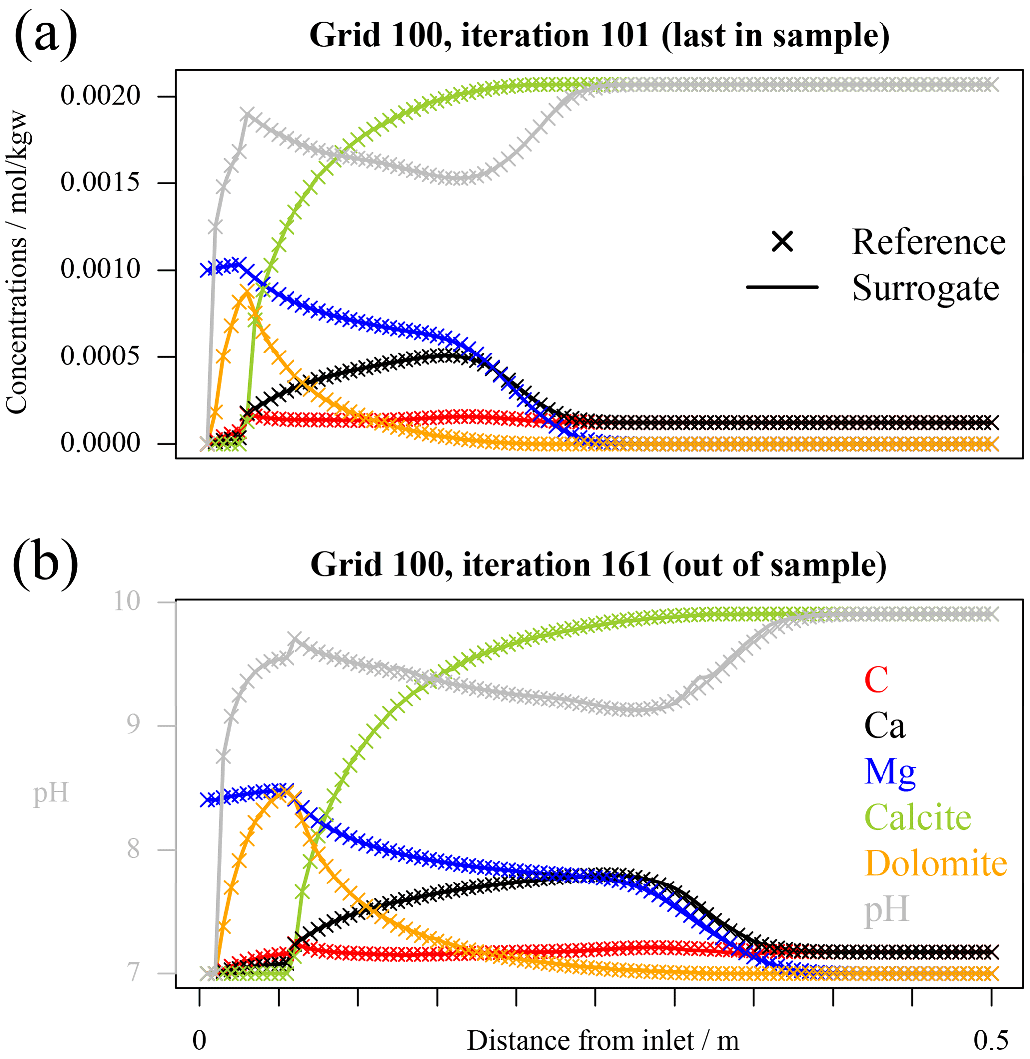
Figure 2Profiles of total concentrations, pH, and minerals for reference and hierarchical coupling 1D simulations with tolerance on mass balance error set to 10−6 for grid 100. The axes are annotated in these figures: all aqueous and mineral concentrations are given in terms of moles per kilogramme of solvent, while pH in its adimensional units. (a) The last in-sample time step; (b) the last simulated time step after 60 iterations for which the surrogate was out-of-sample.
The number of rejected surrogate responses at each time step does not remain constant during the simulations but increases steadily. An overview of all the simulations is given in Fig. 3 (top frame). The more stringent mass balance tolerance of 10−6 (solid lines) obviously rejects many more simulations, which goes hand in hand with the excellent accuracy of the results (Fig. 3, bottom panel; error measured with formula of Eq. 3 excluding pH). It was expected, and it is demonstrated by the evaluation, that starting with the first out-of-sample time step the accuracy of the surrogates significantly drops, which triggers a steep increase in rejected predictions and conversely of calls to PHREEQC. The hierarchical coupling ensures that the errors in the surrogate simulations do not follow the same steep increase, but from this moment on there is a loss of computational efficiency visible in the simulations with tolerance 10−6, which makes all the surrogate predictions actually useless in terms of speedup even before making them so inaccurate to be useless. It is also apparent from the error panel in Fig. 3 (bottom) that errors introduced in the coupled simulations at early time steps propagate through the rest of the simulations so that the overall discrepancy between reference and surrogate simulations also steadily increases. Note that this “diverging behaviour” also tends to bring the geochemistry out-of-sample in the sense of seen vs. unseen geochemical data, since the training data only comprise “physical” input combinations, but, due to the introduced inaccuracies, we are asking the surrogate for more and more predictions based on slightly “unphysical” input combinations. Having highly accurate surrogates would hence also be beneficial in this regard.
It is difficult to discriminate “a priori” between acceptable and unacceptable simulation results based on a threshold of an error measure such as that of Eq. (3), which can be roughly interpreted as “mean percentage error”. This is also a point on which in our opinion further research is needed. Relying on the visualization of the surrogate simulation results and the reference, we can summarize the tolerance on mass balance of 10−6 (solid lines in Fig. 3) as producing accurate coupled simulations, excellent accuracy within the time steps of the training data, and good accuracy after the 60 out-of-sample iterations. The tolerance of 10−5 and the simulations based solely on surrogates produce acceptable accuracy in-sample but unusable and rapidly diverging results out-of-sample.
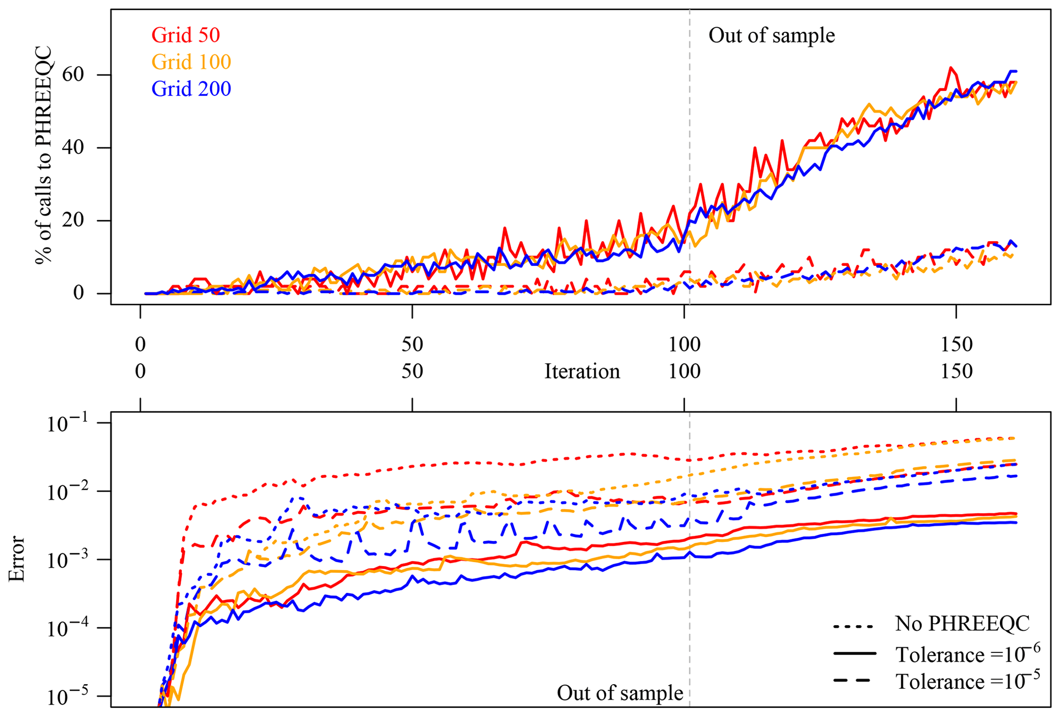
Figure 3Purely data-driven approach: evaluation of calls to full-physics simulator for the runs with hierarchical coupling for the three discretizations at 50, 100, and 200 elements and of overall discrepancy between surrogate simulations and the reference. When the surrogate enters the region of “unseen data”, its accuracy degrades significantly, which causes loss of efficiency rather than accuracy.
For the given chemical problem, the 10−6 tolerance on mass balance could be relaxed, whereas the 10−5 is too optimistic. The optimal value, at least for the considered time steps, lies between these two values.
The overall speedup – in terms of total wall-clock time of the coupled simulations, thus also including CPU time used for advection and all the overheads, although both are much less computationally intensive than chemistry and therefore termed pseudo-speedup – with respect to the reference simulations is summarized in Fig. 4. Here all 161 iterations, including the out-of-sample ones, are considered. Pseudo-speedup increases with grid size as expected. The accurate 10−6 simulations are not accelerated on grid 50 (pseudo-speedup of 0.86), but they reach 1.33 on the 200 grid.

Figure 4Overall pseudo-speedup (total wall-clock time) after 161 iterations for coupled simulations with hierarchical coupling and only relying on the surrogate.
The surrogate-only speedup starts at around 2.6 for the 50 grid and reaches 4.2 for the 200 grid. Considering only the first 101 iterations, the 10−6 simulations would achieve speedup slightly larger than one already on the 50-element grid and would be well over 2 on the 200 grid.
The fully data-driven approach presented above disregards any domain knowledge or known physical relationships between variables besides those which are picked up automatically by the multivariate algorithms operating on the input/outputs in the training data.
We start a second approach by considering the actual “true” degrees of freedom for the geochemical problem, which is fully described by seven inputs and four outputs: Δcalcite, Δdolomite, Cl, and pH. This means that we will have to calculate back the changes in concentrations for C, Ca, and Mg, risking a quicker propagation of errors if the reaction rates of the minerals are incorrectly predicted but honouring by construction the mass balance.
The reference simulations for this part are run with ν=1 and thus without numerical dispersion on four different grids: 50, 100, 200, and 500 elements, respectively. This implies that the simulation on grid 500 has 10 times more coupling iterations than the 50 grid or, in other terms, that the allowable time step in grid 500 is 1 10 of that for grid 50.
A common way to facilitate the task of the regressors by “injecting” physical knowledge into the learning task of the algorithms is to perform feature engineering: this simply means computing new variables defined by non-linear functions of the original ones, which may give further insights regarding multivariate dependencies, hidden conditions, or relevant subsets of the original data.
For any geochemical problem involving dissolution or precipitation of minerals, each mineral's saturation ratio (SR) or its logarithm SI (saturation index) discriminates the direction of the reaction. If SR >1 (and thus SI >0) the mineral is oversaturated and precipitates; it is undersaturated and dissolves if SR <1 (SI <0) and SR =1 (SI =0) implies local thermodynamic equilibrium. Writing the reaction of calcite dissolution as
the law of mass action (LMA) relates, at equilibrium, the activities of the species present in the equation. We conventionally indicate activity with square brackets. For Eq. (5), the LMA reads
where γ stands for the activity coefficient of subscripted aqueous species. The solubility product at equilibrium, tabulated in thermodynamic databases, is a function of temperature and pressure and defines the saturation ratio:
The estimation of the saturation ratio in Eq. (7) using the elemental concentrations available in our training data is the first natural feature engineering we can try. Hereby, a few assumptions must be made.
Using total elemental concentrations as a proxy for species activities implies neglecting the actual speciation to estimate the ion activity products, but also the difference between concentration and activity – true activity [H+] is known from the pH. For the chemical problem at hand, as will be shown, it is a viable approximation, but it will not be in the presence of strong gradients of ionic strength or in general for more complex or concentrated systems. An exception to this simplification is required for dissolved carbon due to the well-known buffer. In this case, given that the whole model is at pH between 7 and 10, we may assume that two single species dominate the dissolved carbon speciation: and . The relationship between the activities of those two species is always kept at equilibrium in the PHREEQC models and thus, up to the “perturbation” due to transport, also in our dataset. This relationship is expressed by the reaction and the corresponding law of mass action written in Eq. (8):
The closure equation, expressing the approximation of total carbon concentration as the sum of two species, gives us the second equation for the two unknowns:
Combining Eqs. 8 and 9, we get the estimation of dissolved bicarbonate (the wide tilde indicates that it is an estimation) from the variables' total carbon and pH comprised in our dataset and an externally calculated thermodynamic constant:
Now we can approximate the theoretical calcite saturation ratio with the formula
The two thermodynamic quantities (at 25 ∘C
and atmospheric pressure) and
were computed with the
CHNOSZ package for the R environment
(Dick, 2019), but may also be derived with simple algebraic
calculations from e.g. the same PHREEQC database employed in the
reactive transport simulations.
Do these two newly defined variables, or “engineered features” (the bicarbonate and calcite saturation ratio), actually help to better understand and characterize our dataset? This can be simply assessed by plotting the Δcalcite against the logarithm of , which is the (Fig. 5a, leftmost panel, dataset from the reference simulations on grid 200, which will be used from now on to illustrate the analysis since it contains enough data points) in the data. While many points remarkably lie on a smooth curve (coloured in black), many others are scattered throughout the graph (in red). It is easy to observe that those red points are either on the trivial Δcalcite =0 line, implying that calcite is undersaturated but not present in the system so nothing happens, or the reaction did not reach the amount which could have been expected based on its initial undersaturation simply because calcite has been completely depleted during the time step. All the red points correspond in fact to simulations with calcite =0 in the labels (results) dataset. The retained black points, however, belong to time steps in which the dissolution of calcite is limited by kinetics and not by its initial amount, and they can thus be used to estimate the reaction rate.
Figure 5a also displays a problem with the defined : its relationship is not bijective with the Δcalcite. This means that we should proceed now to split the data into two different regions above and under the cusp (signalled by the blue horizontal line). However, simply dropping the denominator of Eq. (11) solves this problem to a large extent:
The centre panel in Fig. 5b shows the scatter plot of
Δcalcite versus the simplified
. All points now lie on a smooth curve, and
the relation between the two variables is indeed quite perfectly
bijective, with the exception of points very close to the Δcalcite =0 line, where they are more scattered; but since those
points also correspond to the smallest amounts of reaction, we can
deem this to be a successful approximation. Note that dropping the
denominator in the definition of also means
that this feature does not reach 1 at equilibrium (and
zero), which is clear observing the range
of the x axis in panels (a) and (b) of Fig. 5. This, however, has
no practical consequence for this problem: calcite is always
undersaturated or at equilibrium in the benchmark, and we just defined
a simple feature which is in a bijective relationship with the amount of
true dissolution in the data. While it could be possible to derive
an analytical functional dependency between the observed amount of
dissolved calcite and the estimated , for
example by manipulating the kinetic law, we opted to use a regressor
instead. The good bijectivity between the two variables means that we
should be able to regress the first using only the second. In the
rightmost panel of Fig. 5c the
in-sample predictions of a multivariate adaptive regression
spline (MARS) model are plotted in blue (Friedman, 1991, 1993), which are computed
through the earth R package (Milborrow, 2018) based only
on . The accuracy is already acceptable
indeed; however, by including further predictors from the already
available features, in this case pH, Ca, and Mg, a better regression
(in red) is achieved, improving the RMSE by more than a factor of 2.
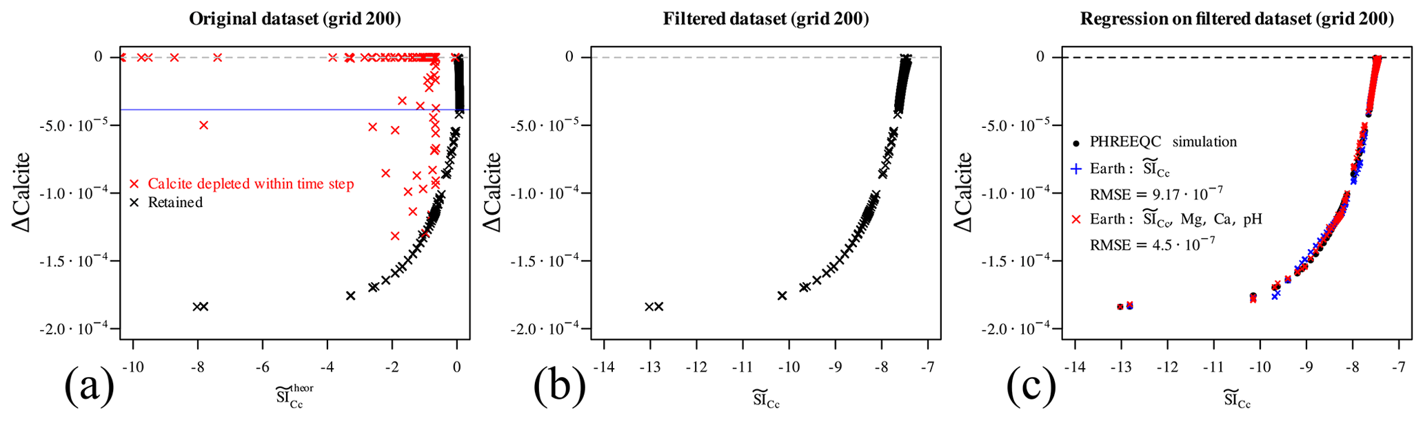
Figure 5(a) Scatter plot of Δcalcite vs. estimated . The data points in red cannot be used to estimate the reaction rate from the dataset since calcite is depleted within the simulation time step. Furthermore, the retained points are not in a bijective relationship with the Δcalcite, with the blue horizontal line separating two regions where bijectivity is given. (b) Δcalcite versus the simplified : bijectivity is achieved. (c) A MARS regressor is computed for the retained data points based solely on the estimated (in blue) and also using other predictors to ameliorate the multivariate regression.
Before moving forward, two considerations are important. First, the red points in Fig. 5a should not be used when trying to estimate the rate of calcite dissolution, since they result from a steep and hidden non-linearity or discontinuity in the underlying model. This is a typical example of data potentially leading to overfitting in a machine-learning sense. Secondly, this “filter” does not need to be applied at runtime during coupled reactive transport simulations: it suffices to correctly estimate the reaction rate given the initial state and then ensure that calcite does not reach negative values.
More interesting and more demanding is the case of dolomite, which firstly precipitates and then re-dissolves in the benchmark simulations. In a completely analogous manner as above we define its saturation ratio as
thus using the total elemental dissolved concentration of C and with resulting from the reaction
The theoretical value of used for calculation of does not discriminate the initially undersaturated from the oversaturated samples (dashed vertical black line in Fig. 6). The “offset” which would serve for a correct discrimination is nothing other than the maximum value of restricted to the region where Δdolomite≤0. We correspondingly update the definition of :
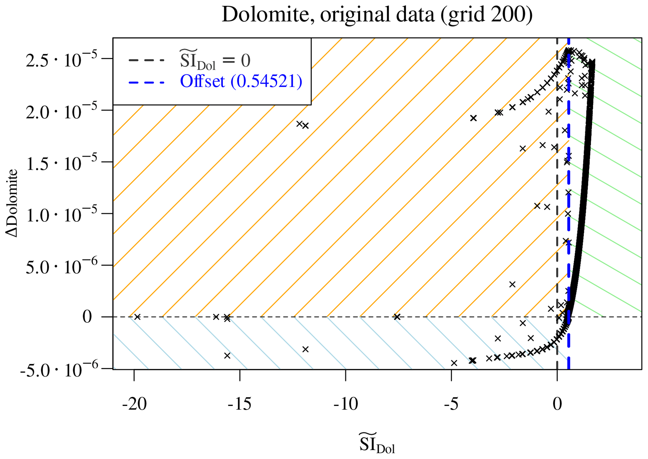
Figure 6Scatter plot of Δdolomite vs. estimated . The theoretical =0 does not discriminate the initially undersaturated from the oversaturated samples (dashed vertical black line) and must be corrected with an apparent offset (blue dashed line). The plot identifies three distinct regions in parameter space: initially supersaturated and precipitating dolomite (top right, green shading), initially undersaturated and dissolving (bottom left, blue shading), and points at which dolomite is initially undersaturated but ends up precipitating (top left, orange shading).
Now we are guaranteed that the vertical line =1 (or equivalently, =0, plotted with a dashed blue line in Fig. 6) correctly divides the parameter space into four distinct quadrants. Note that this offset emerges from the actual considered data and depends on the perturbation of the concentrations due to transport and thus, in our simple advective scheme, on the grid resolution through the time step. It follows that a different offset is expected for the other grids, and a different learning for each grid is necessary.
The green-shaded top right quadrant points to dolomite precipitation in initially supersaturated samples; the bottom left blue-shaded quadrant contains solutions initially undersaturated with respect to dolomite and, if present, dissolving. The top left orange-shaded quadrant is the most problematic: dolomite is initially undersaturated but, presumably due to the concurring dissolution of calcite, it becomes supersaturated during the time step and hence precipitates.
First of all, we note that the initial presence of calcite is a
perfect proxy for . If calcite is initially
present in points reached by the reactive magnesium chloride solution,
then dolomite precipitates. When calcite is completely depleted, then
dolomite starts dissolving again. The dissolution of dolomite in
the absence of calcite follows the same logic as the dissolution of
calcite above: a few points are scattered between the line
Δdolomite =0 and the envelope of points lying on a well-defined curve. These scattered points are again those at which dolomite
is depleted within the time step, so they are excluded. For the
remaining points, an XGBoost regressor based on the predictors
, pH, C, Cl, Mg, and dolomite achieves
excellent accuracy (Fig. 7) in reproducing the observed
Δdolomite.
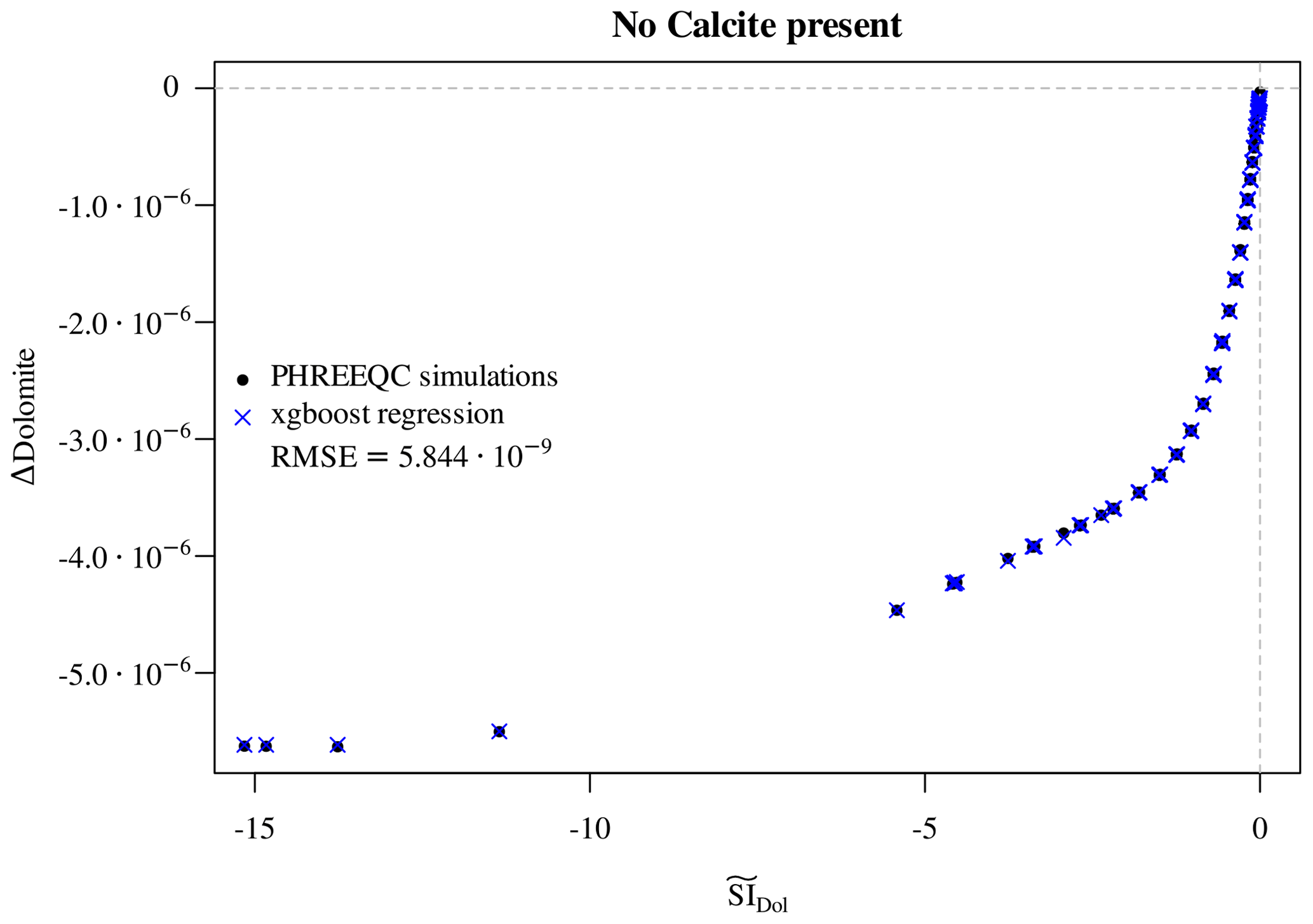
Figure 7Regression of Δdolomite vs. estimated for the cases in which no calcite is initially present. The multivariate regressor makes use of the predictors , pH, C, Cl, Mg, and dolomite.
The top right quadrant of Fig. 6, corresponding to the case of dolomite precipitating while calcite is dissolving, cannot be explained based only on the estimated since their relationship is not surjective (Fig. 8a).

Figure 8Precipitation of dolomite in the presence of calcite. (a) The relationship between Δdolomite and its saturation ratio is not surjective. (b) The ratio perfectly discriminates two distinct regions in parameter space.
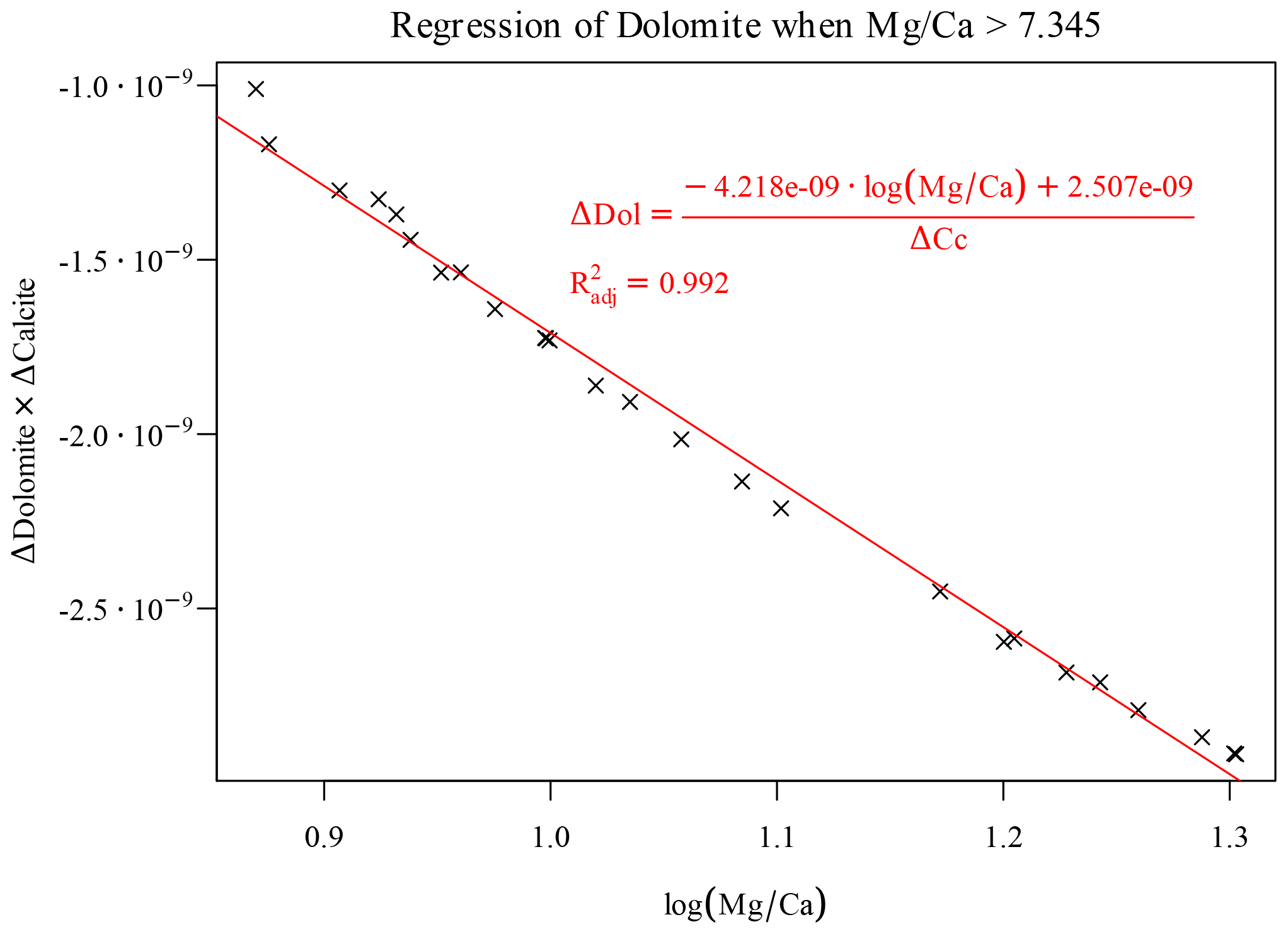
Here again we can use a piece of domain knowledge to engineer a new feature to move forward. The ratio is often used to study the thermodynamics of dissolution of calcite and precipitation of dolomite (Möller and De Lucia, 2020). Effectively, the occurring overall reaction that transforms calcite into dolomite reads
By applying the law of mass action to Eq. (16), it is apparent that its equilibrium constant is a function of the ratio (of its inverse in the form of Eq. 16). Plotting the Δdolomite versus the initial ratio, a particular ratio of 7.345 discriminates between two distinct regions for this reaction. Incidentally, this splitting value corresponds to the highest observed in the training data; again, as previously noted for the offset of the estimated saturation index, this numerical value depends on the considered grid and time step. In the left-hand region we observe a smooth, quasi-linear dependency of the amount of precipitated dolomite on initial . This is a simple bijective relationship to which we can apply a simple monovariate regression. The amount of precipitated dolomite is accurately predicted by a MARS regressor using only as a predictor.
The region on the right of the splitting ratio can be best understood considering the fact that the precipitation of dolomite is limited in this region by a concurrent amount of calcite dissolution. The full-physics chemical solver iteratively finds the correct amounts of calcite dissolution and dolomite precipitation while honouring both the kinetic laws and all the other conditions for a geochemical DAE system (mass action equations, electroneutrality, positive concentrations, activity coefficients). We cannot reproduce such articulate and “interdependent” behaviour without knowing the actual amount of dissolved calcite: we are forced here to employ the previously estimated Δcalcite as a “new feature” to estimate of the amount of dolomite precipitation, albeit limited to this particular region of the parameter space. A surprisingly simple expression, fortunately, captures this relationship quite accurately (Fig. 9).
This implies of course that during coupled simulations first the Δcalcite must be computed, and relying on this value, the Δdolomite can be further estimated.
The last parameter space region left to consider is the orange-shaded, top left quadrant of Fig. 6. Here, although dolomite is undersaturated at the beginning of the time step, it still precipitates in the end, following the concurrent dissolution of calcite, which changes its saturation state. Since, however, we already calculated the Δcalcite, we can update the concentrations of dissolved Ca and C of corresponding amounts. One of these two concentrations, together with that of Mg, will constitute a limiting factor for the precipitation of dolomite. Hence, plotting the Δdolomite against the minimum value of these three concentrations at each point (C must be divided by 2 for the stoichiometry of dolomite), we obtain a piecewise linear relationship with limited non-linear effects. A very simple regression is hence sufficient to capture the bulk of the “true model behaviour” for all these data points (Fig. 10).
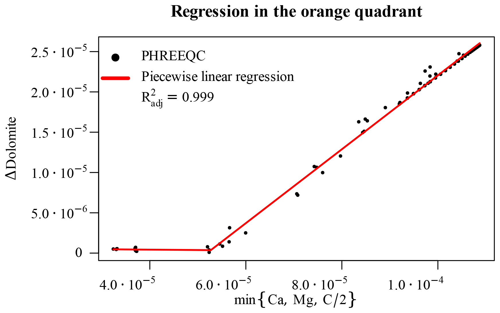
Figure 10Piecewise linear regression for the orange-shaded top left quadrant of Fig. 6 based on the limiting elemental concentration after having considered calcite dissolution.
Now the behaviour of calcite and dolomite is fully understood and we
dispose of a surrogate for both of them. Among the remaining output
variables, only pH needs to be regressed: Cl is non-reactive, meaning
that the surrogate is the identity function. For pH, while it could be
possible to derive a simplified regression informed with geochemical
knowledge, we chose for simplicity to use the XGBoost regressor.
Summarizing, we effectively designed a decision tree based on domain knowledge, which enabled us to make sense of the true data, to perform physically meaningful feature engineering, and ultimately to define a surrogate model “translated” to the data domain (Fig. 11).
The training of this decision tree surrogate consists merely of (1) computing the engineered features, (2) finding the apparent offset for the , (3) finding the split value for the ratio, and (4) performing six distinct regressions on data subsets, three of which are monovariate and two that use fewer predictors than the corresponding completely data-driven counterparts. All of them, excluding pH, only use a subset of the original training dataset. On our workstation, this operation takes a few seconds. The resulting surrogate is valid for the Δt of the corresponding training data.
To evaluate the performance of this surrogate approach, a decision tree is trained separately for each grid (and hence Δt) using the reference time steps until 42 000 s, whereas the coupled simulations are prolonged to 60 000 s so that at least 30 % of the simulation time is computed on unseen geochemical data.
The top panel of Fig. 12 shows the results of the coupled simulation for grid 50 using the surrogate trained on the same data at the end of the iterations used for training. Discrepancies with respect to the reference full-physics simulation are already evident. The problem here is that the training dataset is too small and the time step too large for the decision tree surrogate to be accurate. However, nothing forbids the performance of “inner iterations” for the chemistry using a surrogate trained on a finer grid, which directly corresponds to smaller Δt. For grid 50 (Δt=1066 s) we can hence use the surrogate trained on grid 500 (Δt=106.6 s) just calling it 10 times within each coupling iterations. The bottom panel of Fig. 12 displays the corresponding results.

Figure 11Decision tree for the surrogate based on physical interpretation of the training dataset. The engineered features are used as splits and as predictors for different regressions depending on the region of parameter space. The abbreviations “lm” and “pwl” respectively stand for “linear model” and for “piecewise linear” regression.
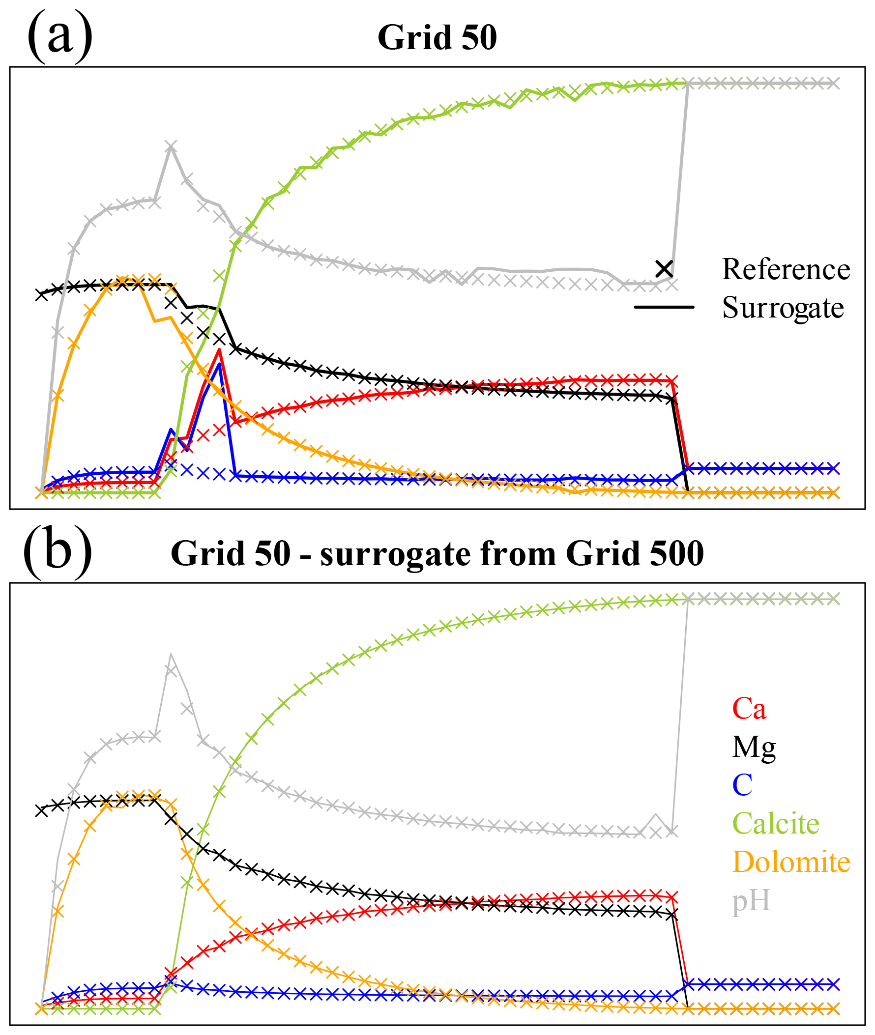
Figure 12Comparison of variable profiles for coupled simulations using the decision tree approach versus the references at the end of the time steps used for training for grid 50 (41 coupled iterations). The axes are the same as in Fig. 2. (a) Decision tree trained on the data from reference grid 50 (Δt=1066 s). (b) Surrogate simulations using a decision tree trained on grid 500 (Δt=106.6 s), repeated 10 times for each coupling time step.
The same problem affects grid 100, which also requires the surrogate trained on grid 500, reiterated five times in this case. Grids 200 and 500 are fine with their own reference data, as can be seen in Fig. 13, this time displaying the end of simulation time at 60 000 s.
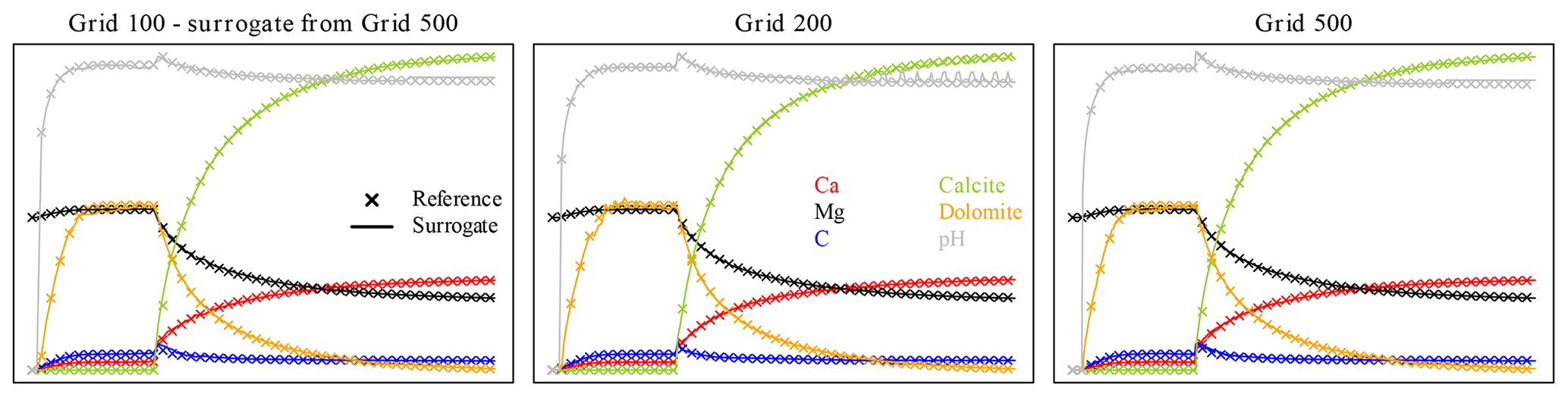
Figure 13Variable profiles after 60 000 s (simulation time) for grids 100, 200, and 500. The axes are the same as in Fig. 2.
In Fig. 14 the errors of the surrogate simulations (top panel) and the overall pseudo-speedup after 60 000 s (bottom panel) are summarized. While inaccuracies are indeed introduced in the coupled simulations by the decision tree surrogate, crossing the out-of-sample boundary does not provoke a steep increase in error. Even if the overall error is slightly larger than the corresponding purely data-driven simulations with 10−6 tolerance, the physics-based approach has the major advantage of being much more robust when encountering unseen data. Moreover, since no calls to PHREEQC are issued at all during these simulations, the performance of the coupled simulations will not degrade during the simulation time. The physics-based surrogates achieve large pseudo-speedups, starting with 2.7 for grid 50 and reaching 6.8 for 500 grid (Fig. 14, bottom panel).
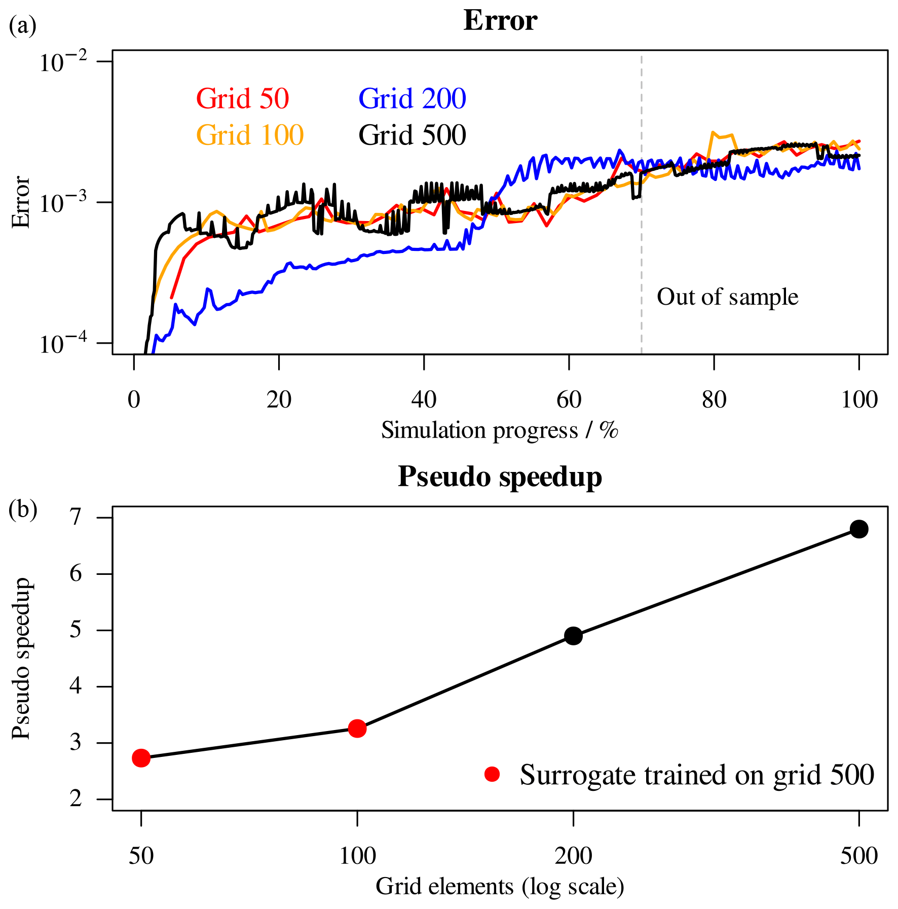
Figure 14(a) Errors of surrogate simulations with respect to references. (b) Overall pseudo-speedup after 60 000 s.
Note that the decision tree approach has been implemented in pure
high-level R language (up to the calls to the regressors
XGBoost and earth, which are implemented in
low-level languages such as C/C++) and is not optimized. A better
implementation would further improve its performance, especially in
the case in which repeated calls to the surrogate are performed at each
coupled iteration.
The results presented in this work devise some strategies which can be exploited to speed up reactive transport simulations. The simplifications concerning the transport and the coupling itself in the present work are obviously severe: stationary, incompressible, and isothermal flow; regular, homogeneous grids; pure advection with a dispersive full explicit forward Euler scheme and constant time stepping that pertain to hydrodynamics. From the point of view of chemistry, there is a lack of feedback on porosity and permeability, an initially homogeneous medium, kinetic rates not depending on reactive surfaces, and the presence of only two reacting minerals. However, while it is still to be assessed how both surrogate approaches will perform once removing these limitations, a number of real-world problems already fall in the complexity class captured by the benchmarks in this work: for example, the modelling of laboratory flow-through reactive transport experiments, which are usually performed in controlled, simplified settings aimed at evaluating kinetic rates, or permeability evolution following from mineral reactions (Poonoosamy et al., 2020).
A fully data-driven approach, combined with a hierarchical coupling in which full-physics simulations are performed only if surrogate predictions are found implausible, is feasible and promises significant speedups for large-scale problems. The main advantage of this approach is that the same “code infrastructure” can be used to replace any physical process, not limited to geochemistry: it is completely general, and it could be implemented in any multiphysics toolbox to be used for any co-simulated process. The hierarchy of models for process co-simulation is a vast research field in itself. This idea has to our knowledge never been implemented specifically for reactive transport, but it has been proposed e.g. for particular problem settings in fluid dynamics and elastomechanics (Altmann, 2013; Altmann and Heiland, 2015) as well as in the broader context of theoretical model reduction and error control (Domschke et al., 2011). This, however, is a fertile interdisciplinary research task, and it is not difficult to foresee that significant progress in this area will soon be required to facilitate and fully leverage the powerful machine-learning algorithms already available in order to speed up any complex, multiscale numerical simulations. The coupling hierarchy implemented in this work cannot be directly compared with the works cited above, since it is merely based on a posteriori evaluation of plausibility of geochemical simulations. Furthermore, it exploits redundant regressions, which is suboptimal, albeit practical: in effects, regressing more variables than strictly necessary is not much different than regressing the true independent variables and their error models. Since the surrogate predictions are so cheap compared to the full physics, it would be only slightly beneficial to first interrogate the error model and then go directly to the full physics instead of computing all the surrogate predictions at once and checking them afterwards. Nevertheless, several improvements can be implemented with respect to the hierarchy presented in this work. The first would be to add charge balance to the error check at runtime. For different classes of chemical processes, other criteria may be required. For example, a check on mass action laws can be implemented for models requiring explicit speciation, like in the simulations of radionuclide diffusion and sorption in storage formations. Another one would be to actually eliminate one or more redundant regressions and base the error check on the accordance between the overlapping one. As an example, one could regress the Δdolomite, Δcalcite, and ΔCa, limiting the mass balance check to one element in practice.
In our opinion there is no point in discussing whether there is one most suitable or most efficient regression algorithm. This largely depends on the problem at hand and on the skills of the modeller. While we rather focused on gradient boosting decision tree regressors for the reasons briefly discussed in Sect. 3, a consistent number of authors have successfully applied artificial neural networks to a variety of geochemical problems and coupled simulations (Laloy and Jacques, 2019; Guérillot and Bruyelle, 2020; Prasianakis et al., 2020). Transforming geochemistry – as for any other physical process – in a pure machine-learning problem requires skills that are usually difficult for geoscientists to acquire, and it fatally overlooks domain knowledge that can be used to improve at least the learning task, which will directly result in accurate and robust predictions, as we demonstrated in Sect. 4. Feature engineering based on known physical relationships and equations should be part of any machine-learning workflow anyway; building experience in this matter by devising suitable strategies for a broad class of geochemical problems is in our opinion much more profitable than trying to tune overly complex black-box models of general applicability. Nevertheless, the popularization of high-level programming interfaces to generate and train such models, specifically addressing hyperparameter tuning with methods such as grid search as well as randomized and Bayesian optimization, mitigates the difficulty that a domain scientist faces when dealing with these problems.
A purely data-driven approach has its own rights and applications. As already noted, it is a completely process-agnostic approach which can be implemented in any simulator for any process. However, in the absence of physical knowledge within the surrogate, the training data must cover all the processes and the scenarios happening in the coupled simulations beforehand. On-demand training and successive incremental update of the surrogates at runtime during the coupled simulations would mitigate this issue. This would require a careful choice of the regressors, since not all of them have this capability, and possibly a sophisticated load balance distribution within the simulator, which is likely viable only in the context of massive parallel computing. In perspective, however, this is a feature that in our opinion should be implemented in the numerical simulators. A second issue, related to the first, is that a data-driven surrogate trained on a specific chemical problem (here meaning initial conditions, concentration of the injected solutions, mineral abundances, time steps) is not automatically transferable to different problem settings, even when, for example, only a single kinetic constant is varied. Again, shaping the surrogate following the physical process to be simulated seems to be the most straightforward way to overcome this issue here, at least partially. One would in fact dispose of regressions in specific parameter space regions which could be parametrically varied following changes in underlying variables. A typical example would be the temperature effect on kinetics, for which the law is of Lasaga type: assuming negligible influence of temperature on a mineral's equilibrium constant and solutes activities, a surrogate expressing the reaction rate at 25 ∘C can be transformed to another temperature by just multiplying it by a factor derived from the Arrhenius term in the original kinetic law.
It remains to be assessed whether and how it is possible to generalize and automate the physics-based surrogate approach devised in Sect. 4 on geochemical problems of higher complexity, i.e. with many minerals reacting. No claim of optimality is made about the actual choice of engineered features we made for this chemical benchmark: different features could possibly explain the data even more simply and thus the chemical process. The important part is the principle: identify relationships as bijective as possible between input and output parameters, compartmentalized in separated regions of parameter space, using features derived by the governing equations. An automation of feature engineering based on stoichiometry of the considered reactions is a straightforward extension, since it can be achieved by simply parsing the thermodynamic database. An automatic application of the approach starting with a large number of engineered features may originate forests of trees much like the well-known random forest or gradient boosting algorithms but specialized in geochemical models: a true hybrid physics–AI model.
Also, the regressors which constitute the leaves of the decision tree in Fig. 11 are completely arbitrary and were selected based on our own experience. A more in-depth breakdown of the relationships between variables, for example analytical expressions derived directly from the kinetic law, could reduce most or all regressions to simple statistical linear models, which would even further increase the interpretability of the surrogate.
In this work fixed time stepping was used for all coupled simulations. A partial extension to variable time stepping has been devised with the inner iteration approach demonstrated with the physics-informed decision tree surrogate: one can recursively call a surrogate on itself, trained on fixed “training Δt” until reaching the “required Δt”. This is obviously valid only for multiples of the training Δt; for non-multiples, some further (non-linear!) interpolation between the inner iterations nearest to the required time step is required. A more flexible and general approach would be treating the time step as a free, independent, and non-negative variable. However, this would require even larger training datasets and hence training times. Assessing an optimal approach for variable time stepping remains high priority for future work.
At the moment no conclusive statement can be made about the general applicability of any surrogate approach to the complex settings usually encountered in practice or the achievable overall speedup – they are strictly too problem- and implementation-dependent to cover them in a general way.
From inhomogeneous irregular grids with transient flow regimes to a highly variable initial spatial distribution of mineralogy and sharp gradients in ionic strengths, these are all factors making the learning task more difficult, either because regression of many more variables (e.g. ionic strength or even activity coefficients) becomes necessary or because much more data are needed in order to obtain coverage of parameter space of higher dimensionality. Embedding domain knowledge into the surrogate seems the most natural way to counter this increase in difficulty. For the second issue, the generation of training data, we believe that the sampling strategy of parameter space used for training should be further optimized. In the simple approach presented in this work – also justified by the fact that we deal with small grids – all the data from the reference simulations were considered, with the only filtering being the removal of duplicated data points. In these datasets many points are concentrated near others, while other regions of parameter space are underrepresented. In problems of increasing complexity and higher dimensionality it becomes paramount to include only data with high informative content in the training dataset to speed up the learning phase. Note that if the training data are taken from reference, true coupled simulations, we are guaranteed that the sampling is always physically plausible – this is not the case if we build the training dataset by pre-computing geochemistry, for example, on a regularly sampled grid covering the whole parameter space. This approach can include physically implausible parameter combinations, which may introduce bias into the surrogate.
Employing surrogates to replace computationally intensive geochemical calculations is a viable strategy to speed up reactive transport simulations. A hierarchical coupling of geochemical subprocesses, allowing for the recurrence of “full-physics” simulations when surrogate predictions are not accurate enough, is advantageous to mitigate the inevitable inaccuracies introduced by the approximated surrogate solutions. In the case of purely data-driven surrogates, which are a completely general approach not limited to geochemistry, regressors operate exclusively on input/output data oblivious to known relationships. Here, redundant information content can be effectively employed to obtain a cheap estimation of the plausibility of surrogate predictions at runtime by checking the errors on mass balance. This estimation works well, at least for the presented geochemical benchmark. Our tests show the consistent advantage of decision-tree-based regression algorithms, especially belonging to the gradient boosting family.
Feature engineering based on domain knowledge, i.e. the actual governing equations for the chemical problem as solved by the full-physics simulator, can be used to construct a surrogate approach in which the learning task is enormously reduced. The strategy consists of partitioning the parameter space based on the engineered features and looking for bijective relationships within each region. This approach reduces both the number of distinct required multivariate predictions and the dimension of the training dataset upon which each regressor must operate. Algorithmically it can be represented by a decision tree and has proved to be both accurate and robust, being equipped to handle unseen data and less sensible to a sparse training dataset, since it embeds and exploits knowledge about the modelled process. Further research is required in order to generalize it and to automate it, to deal with more complex chemical problems, and to adapt it to specific needs such as sensitivity and uncertainty analysis.
Both approaches constitute non-mutually exclusive valid strategies in the arsenal of modellers dealing with the overwhelmingly CPU-expensive reactive transport simulations required by present-day challenges in subsurface utilization. In particular, we are persuaded that hybrid AI–physics models will offer the decisive computational advantage needed to overcome current limitations of classical equation-based numerical modelling.
DecTree v1.0 is a model experiment set up and evaluated in the R environment. All the code used in the present work is available under the LGPL v2.1 licence at Zenodo with DOI https://doi.org/10.5281/zenodo.4569573 (De Lucia, 2021a).
DecTree depends on the RedModRphree package v0.0.4, which is equally
available at Zenodo with DOI https://doi.org/10.5281/zenodo.4569516 (De Lucia, 2021b).
MDL shaped the research, performed analyses and programming, and wrote the paper. MK helped provide funding, shape the research, and revise the paper.
The authors declare that they have no conflict of interest.
Publisher's note: Copernicus Publications remains neutral with regard to jurisdictional claims in published maps and institutional affiliations.
The authors gratefully acknowledge the reviewers for their valuable comments which helped improve the manuscript. Morgan Tranter is also acknowledged for his help in proofreading the manuscript.
This research has been supported by the
Helmholtz-Gemeinschaft in the framework of the project “Reduced
Complexity Models – Explore advanced data science techniques to
create models of reduced complexity” (grant no. ZT-I-0010).
The article processing charges for this open-access publication were covered by the Helmholtz Centre Potsdam – GFZ German Research Centre for Geosciences.
This paper was edited by Havala Pye and reviewed by Paolo Trinchero, Glenn Hammond, and one anonymous referee.
Altmann, R.: Index reduction for operator differential-algebraic equations in elastodynamics, J. Appl. Math. Mech., 93, 648–664, https://doi.org/10.1002/zamm.201200125, 2013. a
Altmann, R. and Heiland, J.: Finite element decomposition and minimal extension for flow equations, ESAIM Math. Model. Numer. Anal., 49, 1489–1509, https://doi.org/10.1051/m2an/2015029, 2015. a
Appelo, C. A. J., Parkhurst, D. L., and Post, V. E. A.: Equations for calculating hydrogeochemical reactions of minerals and gases such as CO2 at high pressures and temperatures, Geochim. Cosmochim. Ac., 125, 49–67, https://doi.org/10.1016/j.gca.2013.10.003, 2013. a, b
Beisman, J. J., Maxwell, R. M., Navarre-Sitchler, A. K., Steefel, C. I., and Molins, S.: ParCrunchFlow: an efficient, parallel reactive transport simulation tool for physically and chemically heterogeneous saturated subsurface environments, Comput. Geosci., 19, 403–422, https://doi.org/10.1007/s10596-015-9475-x, 2015. a
Chen, T. and Guestrin, C.: XGBoost: A Scalable Tree Boosting System, Proceedings of the 22nd ACM SIGKDD International Conference on Knowledge Discovery and Data Mining, https://doi.org/10.1145/2939672.2939785, 2016. a
De Lucia, M.: Chemistry speedup in reactive transport simulations: purely data-driven and physics-based surrogates, Zenodo [code], https://doi.org/10.5281/zenodo.4569574, 2021a. a
De Lucia, M.: RedModRphree: geochemical and reactive transport modelling in R using PHREEQC (Version 0.0.4), Zenodo [code], https://doi.org/10.5281/zenodo.4569516, 2021b. a
De Lucia, M. and Kühn, M.: Coupling R and PHREEQC: Efficient Programming of Geochemical Models, Energy Proced., 40, 464–471, https://doi.org/10.1016/j.egypro.2013.08.053, 2013. a
De Lucia, M., Lagneau, V., Fouquet, C. D., and Bruno, R.: The influence of spatial variability on 2D reactive transport simulations, C. R. Geosci., 343, 406–416, https://doi.org/10.1016/j.crte.2011.04.003, 2011. a
De Lucia, M., Kempka, T., and Kühn, M.: A coupling alternative to reactive transport simulations for long-term prediction of chemical reactions in heterogeneous CO2 storage systems, Geosci. Model Dev., 8, 279–294, https://doi.org/10.5194/gmd-8-279-2015, 2015. a, b
De Lucia, M., Kempka, T., Jatnieks, J., and Kühn, M.: Integrating surrogate models into subsurface simulation framework allows computation of complex reactive transport scenarios, Energy Proced., 125, 580–587, https://doi.org/10.1016/j.egypro.2017.08.200, 2017. a
Dethlefsen, F., Haase, C., Ebert, M., and Dahmke, A.: Uncertainties of geochemical modeling during CO2 sequestration applying batch equilibrium calculations, Environ. Earth Sci., 65, 1105–1117, https://doi.org/10.1007/s12665-011-1360-x, 2011. a
Dick, J. M.: CHNOSZ: Thermodynamic Calculations and Diagrams for Geochemistry, Front. Earth Sci., 7, 180, https://doi.org/10.3389/feart.2019.00180, 2019. a
Domschke, P., Kolb, O., and Lang, J.: Adjoint-Based Control of Model and Discretization Errors for Gas Flow in Networks, International Journal of Mathematical Modelling and Numerical Optimisation, 2, 175–193, https://doi.org/10.1504/IJMMNO.2011.039427, 2011. a
Engesgaard, P. and Kipp, K. L.: A geochemical transport model for redox-controlled movement of mineral fronts in groundwater flow systems: A case of nitrate removal by oxidation of pyrite, Water Resour. Res., 28, 2829–2843, https://doi.org/10.1029/92WR01264, 1992. a
Friedman, J. H.: Multivariate Adaptive Regression Splines (with discussion), Annals of Statistics 19/1, Stanford University, available at: https://statistics.stanford.edu/research/multivariate-adaptive-regression-splines (last access: 23 July 2021), 1991. a
Friedman, J. H.: Multivariate Adaptive Regression Splines (with discussion), Technical Report 110, Stanford University, Department of Statistics, available at: https://statistics.stanford.edu/research/fast-mars (last access: 23 July 2021), 1993. a
Guérillot, D. and Bruyelle, J.: Geochemical equilibrium determination using an artificial neural network in compositional reservoir flow simulation, Comput. Geosci., 24, 697–707, https://doi.org/10.1007/s10596-019-09861-4, 2020. a, b
Hammond, G. E., Lichtner, P. C., and Mills, R. T.: Evaluating the performance of parallel subsurface simulators: An illustrative example with PFLOTRAN, Water Resour. Res., 50, 208–228, https://doi.org/10.1002/2012WR013483, 2014. a
Hassine, A., Masmoudi, A., and Ghribi, A.: Tweedie regression model: a proposed statistical approach for modelling indoor signal path loss, Int. J. Numer. Model. El., 30, e2243, https://doi.org/10.1002/jnm.2243, 2017. a
He, W., Beyer, C., Fleckenstein, J. H., Jang, E., Kolditz, O., Naumov, D., and Kalbacher, T.: A parallelization scheme to simulate reactive transport in the subsurface environment with OGS#IPhreeqc 5.5.7-3.1.2, Geosci. Model Dev., 8, 3333–3348, https://doi.org/10.5194/gmd-8-3333-2015, 2015. a
Huang, Y., Shao, H., Wieland, E., Kolditz, O., and Kosakowski, G.: A new approach to coupled two-phase reactive transport simulation for long-term degradation of concrete, Constr. Build. Mater., 190, 805–829, https://doi.org/10.1016/j.conbuildmat.2018.09.114, 2018. a
Jatnieks, J., De Lucia, M., Dransch, D., and Sips, M.: Data-driven Surrogate Model Approach for Improving the Performance of Reactive Transport Simulations, Energy Proced., 97, 447–453, https://doi.org/10.1016/j.egypro.2016.10.047, 2016. a, b, c
Jørgensen, B.: Exponential Dispersion Models, J. Roy. Stat. Soc. Ser. B, 49, 127–162, https://doi.org/10.2307/2345415, 1987. a
Kelp, M. M., Jacob, D. J., Kutz, J. N., Marshall, J. D., and Tessum, C. W.: Toward Stable, General Machine-Learned Models of the Atmospheric Chemical System, J. Geophys. Res.-Atmos., 125, e2020JD032759, https://doi.org/10.1029/2020jd032759, 2020. a
Laloy, E. and Jacques, D.: Emulation of CPU-demanding reactive transport models: a comparison of Gaussian processes, polynomial chaos expansion, and deep neural networks, Comput. Geosci., 23, 1193–1215, https://doi.org/10.1007/s10596-019-09875-y, 2019. a, b, c
Leal, A. M. M., Kyas, S., Kulik, D. A., and Saar, M. O.: Accelerating Reactive Transport Modeling: On-Demand Machine Learning Algorithm for Chemical Equilibrium Calculations, Transport Porous Med., 133, 161–204, https://doi.org/10.1007/s11242-020-01412-1, 2020. a, b, c
Marty, N. C., Claret, F., Lassin, A., Tremosa, J., Blanc, P., Madé, B., Giffaut, E., Cochepin, B., and Tournassat, C.: A database of dissolution and precipitation rates for clay-rocks minerals, Appl. Geochem., 55, 108–118, https://doi.org/10.1016/j.apgeochem.2014.10.012, 2015. a
Milborrow, S.: earth: Multivariate Adaptive Regression Splines derived from mda::mars, edited by: Hastie, T. and Tibshirani, R., r package, available at: https://CRAN.R-project.org/package=earth (last access: 23 July 2021), 2018. a
Moog, H., Bok, F., Marquardt, C., and Brendler, V.: Disposal of nuclear waste in host rock formations featuring high-saline solutions – Implementation of a thermodynamic reference database (THEREDA), Appl. Geochem., 55, 72–84, https://doi.org/10.1016/j.apgeochem.2014.12.016, 2015. a
Möller, P. and De Lucia, M.: The impact of Mg2+ ions on equilibration of Mg-Ca carbonates in groundwater and brines, Geochemistry, 80, 125611, https://doi.org/10.1016/j.chemer.2020.125611, 2020. a, b
Nissan, A. and Berkowitz, B.: Reactive Transport in Heterogeneous Porous Media Under Different Péclet Numbers, Water Resour. Res., 55, 10119–10129, https://doi.org/10.1029/2019wr025585, 2019. a
Palandri, J. L. and Kharaka, Y. K.: A compilation of rate parameters of water-mineral interaction kinetics for application to geochemical modeling, Tech. rep., USGS Menlo Park, California, USA, 2004. a
Parkhurst, D. L. and Wissmeier, L.: PhreeqcRM: A reaction module for transport simulators based on the geochemical model PHREEQC, Adv. Water Resour., 83, 176–189, https://doi.org/10.1016/j.advwatres.2015.06.001, 2015. a
Poonoosamy, J., Klinkenberg, M., Deissmann, G., Brandt, F., Bosbach, D., Mäder, U., and Kosakowski, G.: Effects of solution supersaturation on barite precipitation in porous media and consequences on permeability: Experiments and modelling, Geochim. Cosmochim. Ac., 270, 43–60, https://doi.org/10.1016/j.gca.2019.11.018, 2020. a
Prasianakis, N. I., Haller, R., Mahrous, M., Poonoosamy, J., Pfingsten, W., and Churakov, S. V.: Neural network based process coupling and parameter upscaling in reactive transport simulations, Geochim. Cosmochim. Ac., 291, 126–143, https://doi.org/10.1016/j.gca.2020.07.019, 2020. a, b, c
Prommer, H., Sun, J., and Kocar, B. D.: Using Reactive Transport Models to Quantify and Predict Groundwater Quality, Elements, 15, 87–92, https://doi.org/10.2138/gselements.15.2.87, 2019. a
R Core Team: R: A Language and Environment for Statistical Computing, R Foundation for Statistical Computing, Vienna, Austria, available at: https://www.R-project.org/ (last access: 23 July 2021), 2020. a
Shao, H., Dmytrieva, S. V., Kolditz, O., Kulik, D. A., Pfingsten, W., and Kosakowski, G.: Modeling reactive transport in non-ideal aqueous–solid solution system, Appl. Geochem., 24, 1287–1300, https://doi.org/10.1016/j.apgeochem.2009.04.001, 2009. a
Steefel, C. I.: Reactive Transport at the Crossroads, Rev. Mineral. Geochem., 85, 1–26, https://doi.org/10.2138/rmg.2019.85.1, 2019. a
Steefel, C. I., DePaolo, D. J., and Lichtner, P. C.: Reactive transport modeling: An essential tool and a new research approach for the Earth sciences, Earth Planet. Sc. Lett., 240, 539–558, https://doi.org/10.1016/j.epsl.2005.09.017, 2005. a
Steefel, C. I., Appelo, C. A. J., Arora, B., Jacques, D., Kalbacher, T., Kolditz, O., Lagneau, V., Lichtner, P. C., Mayer, K. U., Meeussen, J. C. L., Molins, S., Moulton, D., Shao, H., Šimůnek, J., Spycher, N., Yabusaki, S. B., and Yeh, G. T.: Reactive transport codes for subsurface environmental simulation, Comput. Geosci., 19, 445–478, https://doi.org/10.1007/s10596-014-9443-x, 2015. a, b
Tweedie, M. C. K.: An index which distinguishes between some important exponential families. Statistics: Applications and New Directions, Proceedings of the Indian Statistical Institute, Golden Jubilee International Conference, Golden Jubilee International Conference, edited by: Ghosh, J. K. and Roy, J., Indian Statistical Institute, Statistics: Applications and New Directions, Calcutta, 579–604, 1984. a
- Abstract
- Introduction
- Methods: simulation environment and benchmark problem
- Fully data-driven approach
- Surrogates based on geochemical knowledge
- Discussion and future work
- Conclusions
- Code availability
- Author contributions
- Competing interests
- Disclaimer
- Acknowledgements
- Financial support
- Review statement
- References
full-physicssimulations are called only if the surrogate predictions are implausible. Furthermore, we devise and evaluate a decision tree surrogate approach designed to inject domain knowledge of the surrogate by defining engineered features based on law of mass action or stoichiometric reaction equations.
- Abstract
- Introduction
- Methods: simulation environment and benchmark problem
- Fully data-driven approach
- Surrogates based on geochemical knowledge
- Discussion and future work
- Conclusions
- Code availability
- Author contributions
- Competing interests
- Disclaimer
- Acknowledgements
- Financial support
- Review statement
- References