Impact of Initialized Land Surface Temperature and Snowpack on Subseasonal to Seasonal Prediction Project, Phase I (LS4P-I): organization and experimental design

Subseasonal-to-seasonal (S2S) prediction, especially the prediction of extreme hydroclimate events such as droughts and floods, is not only scientifically challenging, but also has substantial societal impacts. Motivated by preliminary studies, the Global Energy and Water Exchanges (GEWEX)/Global Atmospheric System Study (GASS) has launched a new initiative called “Impact of Initialized Land Surface Temperature and Snowpack on Subseasonal to Seasonal Prediction” (LS4P) as the first international grass-roots effort to introduce spring land surface temperature (LST)/subsurface temperature (SUBT) anomalies over high mountain areas as a crucial factor that can lead to significant improvement in precipitation prediction through the remote effects of land–atmosphere interactions. LS4P focuses on process understanding and predictability, and hence it is different from, and complements, other international projects that focus on the operational S2S prediction. More than 40 groups worldwide have participated in this effort, including 21 Earth system models, 9 regional climate models, and 7 data groups.

This paper provides an overview of the history and objectives of LS4P, provides the first-phase experimental protocol (LS4P-I) which focuses on the remote effect of the Tibetan Plateau, discusses the LST/SUBT initialization, and presents the preliminary results. Multi-model ensemble experiments and analyses of observational data have revealed that the hydroclimatic effect of the spring LST on the Tibetan Plateau is not limited to the Yangtze River basin but may have a significant large-scale impact on summer precipitation beyond East Asia and its S2S prediction. Preliminary studies and analysis have also shown that LS4P models are unable to preserve the initialized LST anomalies in producing the observed anomalies largely for two main reasons: (i) inadequacies in the land models arising from total soil depths which are too shallow and the use of simplified parameterizations, which both tend to limit the soil memory; (ii) reanalysis data, which are used for initial conditions, have large discrepancies from the observed mean state and anomalies of LST over the Tibetan Plateau. Innovative approaches have been developed to largely overcome these problems.

1 Introduction

Subseasonal-to-seasonal (S2S) prediction, especially the prediction of extreme hydroclimatic events such as droughts and floods, is not only scientifically challenging, but also has substantial societal impacts since such phenomena can have serious agricultural, economic, and ecological consequences (Merryfield et al., 2020). However, the prediction skill for precipitation anomalies in spring and summer months, a significant component of extreme climate events, has remained stubbornly low for years. It is therefore important to understand the sources of such predictability and to develop more reliable monitoring and prediction capabilities. Various mechanisms have been attributed to S2S predictability. For instance, oceanic basin-wide tropical sea surface temperature (SST) anomalies are known to play a major role in causing extreme events. The connection between SST (e.g., El Niño–Southern Oscillation, ENSO, Pacific Decadal Oscillation, PDO, Atlantic Multidecadal Oscillation, AMO, and Madden–Julian oscillation, MJO) and the associated weather and climate predictability has been extensively studied for decades (Trenberth et al., 1988; Ting and Wang, 1997; Barlow et al., 2001; Schubert et al., 2008; Jia and Yang, 2013; Seager et al., 2014). The linkage of extreme hydrological events to tropical ocean basin SST anomalies allows us to predict them with useful skill at long lead times ranging from a few months to a few years. Despite significant correlations and demonstrated predictive value, numerous studies based on observational data analyses and numerical simulations have consistently shown that SST alone only partially explains the phenomena of predictability (Rajagopalan et al., 2000; Schubert et al., 2004, 2009; Scaife et al., 2009; Mo et al., 2009; Rui and Wang, 2011; Pu et al., 2016; Xue et al., 2016a, b, 2018; Orth and Seneviratne, 2017). For instance, the 2015–2016 El Niño event, one of the strongest since 1950, was associated with an extraordinary Californian drought, while the 2016–2017 La Niña event has been related to record rainfall that effectively ended the 5-year Californian drought, contrary to established canonical SST–Californian drought/flood relationships. In South America, there is also an example where the canonical association of thermally direct, SST-driven atmospheric circulation fails (Robertson and Mechoso, 2000; Nobre et al., 2012). Although an important role for random atmospheric internal variability in such extreme events has been proposed (Hoerling et al., 2009), such exceptions in explaining vital hydroclimatic extreme events as well as low prediction skill underscore the need to seek explanations beyond current traditional approaches. It is therefore imperative to explore other avenues to improve S2S prediction skill.

Studies have demonstrated that the predictive ability of models may come from their ability to represent land surface features that have inertia, such as vegetation (evolving cover and density), soil moisture and snow (e.g., Xue et al., 1996a, 2010b; Lu et al., 2001; Delire et al., 2004; Koster et al., 2004, 2006; Gastineau et al., 2017). Most land–atmosphere interaction studies have focused on local effects, for instance, such as those in the previous Global Land-Atmosphere Coupling Experiment (GLACE) (Koster et al., 2006). The possible remote (nonlocal) effects of large-scale spring land surface/subsurface temperature (LST/SUBT) anomalies in geographical areas upstream of the areas which experience late spring–summer drought/flood, an underappreciated relation, were largely ignored until recent preliminary modeling and data analysis studies revealed the important role of high mountain LST/SUBT in S2S predictability: this discovery has stimulated research in this direction. For instance, observational data in the Tibetan Plateau and the Rocky Mountains have shown that land surface temperature anomalies can be sustained for entire seasons and that they are accompanied by persistent subsurface temperature, snow, and albedo anomalies (Liu et al., 2020). Since only 2 m air temperature (T-2m) has significant global coverage and since its values are very close to LST in stations with measurements for both (Liu et al., 2020; also see the discussion in Sect. 5.1), observed T-2m data have been used in diagnostic studies to identify spatial and temporal characteristics of land surface temperature variability and its relationship with other climate variables. Figure 1 exhibits the persistence of the monthly mean difference of T-2m between warm and cold Mays, which are selected based on a threshold of 0.5 standard deviation during the period 1981–2010. Please note that the warm and cold years that are selected based on May values are applied to other months in the figure. Those anomalies can persist for several months, especially during the spring. Preliminary studies have been carried out to explore the relationship between spring LST/SUBT anomalies and summer precipitation anomalies in downstream regions in North America and East Asia (Xue et al., 2002, 2012, 2016b, 2018; Diallo et al., 2019). Data analyses from these studies identify significant correlations between springtime T-2m cold (warm) anomalies in both the Rocky Mountains and Tibetan Plateau and respective downstream drought (flood) events in late spring/summer. Modeling studies using the NCEP Global Forecast System (GFS, Xue et al., 2004) and the regional climate model version of Weather Research and Forecasting (WRF; Skamarock et al., 2008), both of which were coupled to a land model Simplified Simple Biosphere Model (SSiB, Xue et al., 1991; Zhan et al., 2003) using observed T-2m and reanalysis data as constraints, have also suggested that there is a remote effect of land temperature changes in the Rocky Mountains and the Tibetan Plateau on their respective downstream regions with a magnitude comparable with the more familiar effects of SST and atmospheric internal variability. Recent studies have further revealed the presence of LST/SUBT effects in other seasons and regions (Shukla et al., 2019). These studies have stimulated the scientific community's interest in pursuing this issue further with multi-model experiments, which will be discussed in the next section.

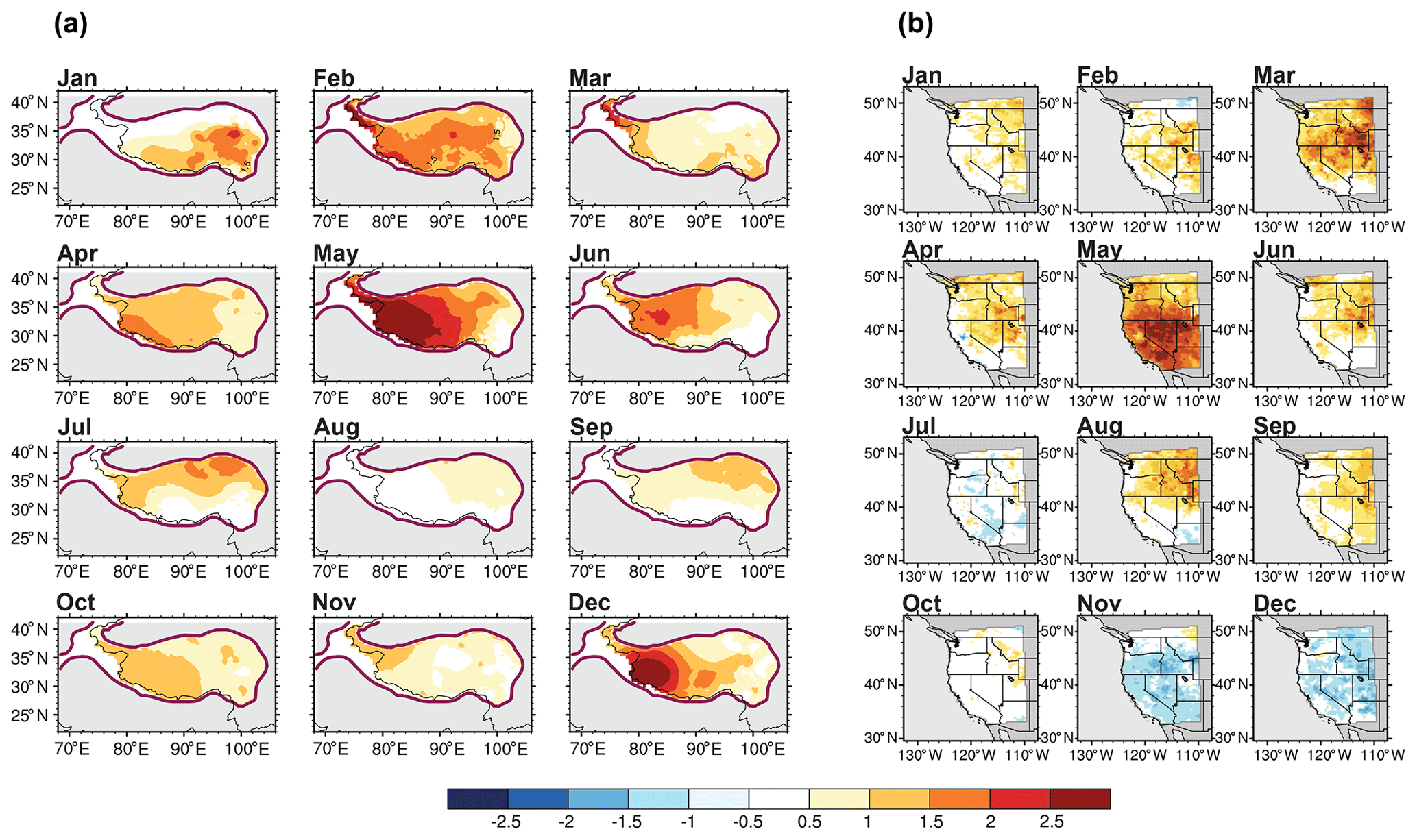
Figure 1 Monthly 2 m temperature difference between warm and cold years (^∘C). (a) Over the Tibetan Plateau based on the CMA data; (b) over the western US based on NARR data. Notes. (1) Years for the Tibetan Plateau and western US are selected based on their May anomalies, respectively, using a threshold of 0.5 standard deviation during the period 1981–2010. The differences between these warm and cold years are applied for all months. (2) The North American Regional Reanalysis (NARR, Mesinger et al., 2006) assimilated the observed 2 m temperature and is viewed as having an accurate representation of the observed surface air temperature.

The main hypothesis of LS4P is that LST and SUBT anomalies in early spring carry information about the energy and water balances in frozen ground, which is related to the amount of snow/ice on the ground and in the frozen soil layer below that is melted in late spring and early summer as well as the thermal status from the preceding winter, which has a long memory. The more snow/ice on the ground and in the frozen soil layer, the longer the seasonal transition from spring to summer. The timing of such a seasonal transition over high-elevation areas in the western part (upstream) of the land mass plays an important role in setting up the circulation pattern downstream over the lower-elevation areas to the east. The strength as well as the duration of LST/SUBT interactions with downstream circulation patterns should affect the occurrence of droughts or floods in late spring/summer over the eastern parts of the continents.

A number of studies have also started to pursue the potential causes of the spring LST/SUBT anomaly in the Tibetan Plateau and the Rocky Mountains. Analyses based on observational station data over the Tibetan Plateau show that the LST anomaly is highly correlated with anomalous snow, surface albedo and SUBT in the preceding months. Using data from an offline model incorporating permafrost processes (Li et al., 2010) and driven with observed meteorological data as forcing over the Tibetan Plateau, a regression model can predict a LST anomaly at the monthly and seasonal scales with surface albedo and mid-layer (40–160 cm) SUBT as predictors (Liu et al., 2020). Additional analyses using observational data show that the spring LST in the Tibetan Plateau is significantly coupled with the regional snow cover in the preceding months. The latter is also strongly coupled with February atmospheric circulation patterns and wave activity at mid to high latitudes (Zhang et al., 2019). Moreover, a modeling study focusing on North America (Broxton et al., 2017) showed that snow water equivalent (SWE) anomalies more strongly affect April–June temperature forecasts than SST anomalies. It is likely that a temporary filtered response to snow anomalies may be preserved in the LST and SUBT anomalies, and this mechanism deserves further investigation. Additional research on the causes of LST/SUBT anomalies would likely help us to better understand the sources of S2S predictability.

One factor that is closely related to the LST/SUBT anomaly is light-absorbing particles (LAPs) in snow. In particular, the snow-darkening effect by LAPs in snow due to deposition of aerosols, e.g., desert dust, black carbon and organic carbon from industrial pollution, biomass burning, and nearby wildfires, can reduce snow albedo, which increases the absorption of solar radiation by the land surface. This enhanced energy absorption can alter the surface energy balance, leading to anomalous T-2m and snowmelt during the boreal spring. Recent studies have shown that the snow-darkening effect can lead to large increases in surface temperature over the Tibetan Plateau in April–May, thereby strongly affecting the subsequent evolution of the jet stream and variability of summertime precipitation over India, East Asia, and Eurasia (Lau and Kim, 2018; Rahimi et al., 2019; Sang et al., 2019). At present, the representations of snow amount, coverage, and LAPs in snow are either absent or grossly inadequate in most climate models, especially in high mountain regions. This could be one of the major reasons for the large discrepancies in simulated T-2m and its anomaly in current Earth system models (ESMs).

In the following text, Sect. 2 introduces the historical development of the initiative “Impact of Initialized Land Surface Temperature and Snowpack on Subseasonal to Seasonal Prediction” (LS4P) and its research objectives. Section 3 presents the LS4P Phase I protocol (LS4P-I): its experimental design and model output requirements. Section 4 discusses causes of current LS4P-I models' deficiencies in preserving land memory and possible approaches for improvement. Section 5 briefly presents some preliminary LS4P-I results and discusses the future plan and perspectives.

2 Development of the initiative on “Impact of initialized Land Surface temperature and Snowpack on Subseasonal to Seasonal Prediction” (LS4P) and its link to other S2S prediction programs

Although T-2m measurement has the longest meteorological observational record with global coverage and the best quality among various land surface variables, its application in S2S prediction has largely been overlooked. Preliminary experiments to test the impact of model initialization of LST/SUBT on the S2S prediction as presented in the previous section are encouraging, but the results were obtained from only one ESM and one RCM, with North America and East Asia as the focus regions (Xue et al., 2016b, 2018). Due to the existing shortcomings and uncertainties associated with individual models, it is imperative to have a multi-model approach in order to further test the LST-memory hypothesis and to explore predictability in more regions. Furthermore, since LS4P proposes a new approach, involving a decade-long effort to explore, test, and understand the concept as well as to develop a proper methodology for the use of ESMs and RCMs, it is also imperative to disseminate information related to the LST/SUBT approach, including lessons learned and experience, such that more research groups can understand the approach/methodology and test the LST/SUBT effect.

With the preliminary results revealing the promising use of T-2m for LST/SUBT S2S prediction, thereby opening a new gateway for improving S2S prediction, the Global Energy and Water Exchanges (GEWEX) and GEWEX/Global Atmospheric System Study (GASS) have supported the establishment of the new initiative called LS4P. The idea for the new initiative was first presented at the 2nd Pan-GASS meeting in Lorne, Australia, in February 2018. The initiative was introduced to the GEWEX community at the GEWEX Open Science Conference in Canmore, Canada, in May 2018.

Since the inception of the LS4P in December 2018, more than 40 groups worldwide have participated in this effort, including 21 ESM groups, many of which are from major climate research centers, 9 RCM groups, and 7 data groups. A description of the major components of each of the ESM and RCM models is summarized in Appendix A. The main data products that are relevant to the LS4P research from the data group are presented in Sect. 3.1. A complete listing of LS4P group information can be found at https://ls4p.geog.ucla.edu/ (last access: 1 June 2021). Because LS4P takes a new approach in S2S prediction, GEWEX, the Third Pole Environment (TPE), and the U.S. National Science Foundation supported two workshops at the American Geophysical Union Fall Meetings in December 2018 and December 2019 and another one at Nanjing University, China, in July 2019. The workshop goals were to discuss and develop the project and to provide training for the modeling groups to better understand and practice the LST/SUBT approach (Xue et al., 2019a, b).

The LS4P activities are closely related to a number of ongoing international projects. S2S prediction is the topic of a joint project of the World Weather Research Program (WWRP) and World Climate Research Program (WCRP), which aim to improve understanding and forecast skill at the S2S timescale, between 2 weeks and a season (WMO, 2013; Vitart et al., 2017; Merryfield et al., 2020). Their S2S project has the study of land initialization and configuration as one of its major activities. The LS4P research activities to address these scientific challenges are consistent with those of the WWRP/WCRP S2S project. The LS4P activity is also closely related to the TPE program. The TPE has closely worked with LS4P to provide and maintain a database to support this project, which is discussed in Sect. 3.1 and Appendices C and D. The first phase of LS4P will be a joint effort with the TPE Earth System Model Inter-comparison Project (TPEMIP), which focuses on regional-scale Earth system modeling over the high-elevation Tibetan Plateau region. The LS4P initiative is also relevant to GEWEX Global Land Atmosphere System Study (GLASS) panel objectives because estimating the contribution of land memory to atmospheric predictability from convective to seasonal timescales is one of its main themes. This requires an understanding of the key physical interactions between the land and the atmosphere and how feedbacks can change the subsequent evolution of both the atmosphere and the land state. The focus of LS4P on soil temperature also complements GLASS' research on the role of soil moisture as it pertains to land–atmosphere coupling and predictability. LS4P has interacted with these project groups and developed the experiments which support and complement their planned research activities.

This LS4P project intends to address the following questions.

• What is the impact of initializing large-scale LST/SUBT and LAPs in snow in climate models on S2S prediction in different regions?

• What are the relative roles and uncertainties of the associated land processes compared with those of the ocean state in S2S prediction? How do they synergistically enhance S2S predictability?

LS4P focuses on process understanding and predictability, and hence it is different from, and complements, other international projects that focus on the operational S2S prediction. The majority of the models participating in LS4P are ESMs, although there is a good number of RCMs involved. Some difficulties have been identified regarding how to apply RCMs for studying the LST/SUBT effect (Xue et al., 2012). The main concern is that imposition of the same lateral boundary conditions (LBCs) for an RCM's control and anomaly runs may hamper the necessary modification of circulations at larger scales in the anomaly run. This issue will be more comprehensively studied in LS4P using a much larger RCM domain configuration to reduce the LBC control on the large-scale change.

The project will ultimately consist of several phases, each of which will focus on a particular high mountain region on one continent as a focal point. The LS4P-I will investigate the LST/SUBT effect in the Tibetan Plateau. The second phase of LS4P will focus on the Rocky Mountains of North America. It is intended that this project will also provide motivation for examining additional high mountains on other continents with similar geographic structures, such as those in South America, for the potential of the LST/SUBT effect to provide added value to S2S prediction and understanding of the pertinent physical principles. Since Phase I is mainly looking for first-order effects most related to the soil surface and deeper layers, the effect of LAPs in snow in high mountain regions will not be included in the Phase I experiments except for some individual group efforts, and therefore they will not be presented further in this paper.

3 LS4P First Phase Experiment Protocol: remote effects of Tibetan Plateau LST/SUBT

The Tibetan Plateau region provides an ideal geographic location for the LS4P-I test owing to its relatively high elevation and large scale (areal extent) as well as the presence of persistent LST anomalies. The Tibetan Plateau provides thermal and dynamic forcings which drive the Asian monsoon through a huge, elevated heat source in the middle troposphere, and this has been reported in the literature for decades (e.g., Ye, 1981; Yanai et al., 1992; Wu et al., 2007; Wang et al., 2008; Yao et al., 2019). Thus, a large impact of the Tibetan Plateau LST/SUBT anomaly effect should be expected and has been demonstrated in a preliminary test (Xue et al., 2018).

3.1 Observational data for LS4P Phase I (LS4P-I)

The observational data provide the foundation for the LS4P research, are used for the LS4P model initialization of surface and boundary conditions, validation, and other relevant research activities, and are listed in Appendix B. Moreover, there are large amounts of observational data available in the Tibetan Plateau area, which are produced by the data groups, which are participating in LS4P and are available for the community to conduct further LS4P-related research, such as studying the causes of the LST/SUBT anomalies, the characteristics of the surface and atmospheric processes in the Tibetan Plateau, etc.

The TPE has conducted comprehensive measurements over the Tibetan Plateau for more than a decade and has integrated the observational data into the National Tibetan Plateau Data Center (Li et al., 2020), which has more than 2400 different data sets for scientific research focused on the Tibetan Plateau. Featured data sets of high mountainous observations on the Tibetan Plateau include those from the High-cold region Observation and Research Network for Land surface processes and Environment of China (HORN), which contains the meteorological, hydrological and ecological data sets (Peng and Zhu, 2017), soil temperature and moisture observations (Su et al., 2011; Yang et al., 2013), multi-scale observations of the Heihe River basin (Li et al., 2017; Liu et al., 2018; Che et al., 2019; Li et al., 2019), and multiple data sets from the coordinated Asia–European long-term observing system for the Tibetan Plateau (Ma et al., 2009).

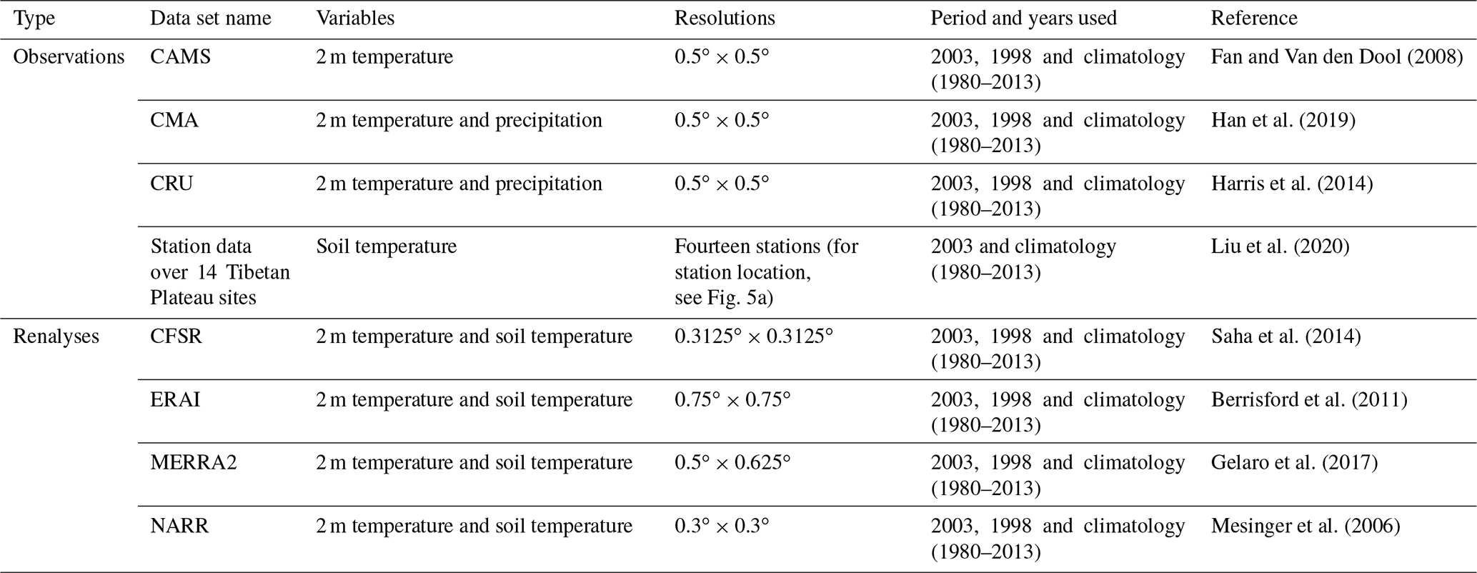
The Third Tibetan Plateau Atmospheric Scientific Experiment (TIPEX-III, Zhao et al., 2018) also provides field measurement data for the LS4P project. The Chinese Meteorological Administration (CMA) provides some field measurements with long-term records. The observed CMA monthly mean precipitation and T-2m and topography data, with a 0.5^∘ resolution based on station measurements (Han et al., 2019; X. Liang et al., 2020), are used in LS4P to evaluate the LS4P models' performance over the Tibetan Plateau and to help produce the LST/SUBT mask for model initialization (see Sect. 4.2 for details). There are 80 stations over the Tibetan Plateau covering the period from 1961 to 2017. Among them, 14 stations have soil temperature measurements reaching a depth of 320 cm. After 2006, more station data are available from the TPE. A detailed spatial interpolation method for the data sets is discussed in Han et al. (2019). This is in contrast with most ground stations around the world, which only include measurements for shallow soil layers, e.g., only reaching down to 101.6 cm (Hu and Feng, 2004). Because of the lack of subsurface measurements, there has been some speculation as to whether the LST/SUBT anomaly and memory as well as the hypothesized relationship between T-2m, LST and SUBT truly exist in the real world. These data provide crucial information to support LS4P-related research (e.g., Liu et al., 2020; Li et al., 2021).

In addition to the ground measurements, satellite products from 1981 to 2018 from the GLASS (S. Liang et al., 2013, 2020) data set will also be employed for this project. This data set consists of surface skin temperature, albedo, emissivity, surface radiation components and vegetation conditions (http://www.glass.umd.edu, last access: 1 June 2021).

3.2 Experimental design: baseline and sensitivity experiments

This section describes the standard design and configuration for the LS4P-I experiment, which consists of four tasks (Table 1). May and June 2003 are the time periods which have been selected for the main tests. The summer of 2003 was characterized by a severe drought over the southern part of the Yangtze River basin in eastern China, with an average anomalous precipitation rate of −1.5 mm/day over the area bounded by 112–121^∘ E and 24–30^∘ N.¹ The drought resulted in 100 × 10⁶ kg crop yield losses, along with an economic loss of 5.8 billion Chinese Yuan (Zhang and Zhou, 2015). To the north of the Yangtze River, there was above-normal precipitation, with anomaly precipitation rates of 1.32 mm/day over the area within 112–121^∘ E and 30–36^∘ N.² Over the same time period, observational data show a cold spring over the Tibetan Plateau; the average T-2m in May above 4000 m was about −1.4 ^∘C below the climatological average. Maximum covariance analysis (MCA, Wallace et al., 1992; von Storch and Zwiers, 1999) showed a positive/negative lag correlation between the May T-2m anomaly in the Tibetan Plateau and a June precipitation anomaly to the south (north) of the Yangtze River. Meanwhile, a preliminary modeling study revealed the causal relationship between the May T-2m/LST/SUBT anomaly over the Tibetan Plateau and the June drought/flood in East Asia (Xue et al., 2018). LS4P intends to further test and confirm such causal relationships with multiple state-of-the-art ESMs in order to assess the uncertainty and to compare the T-2m/LST/SUBT effect with that of the ocean state.

Table 1 Summary of different tasks under the LS4P-I framework.

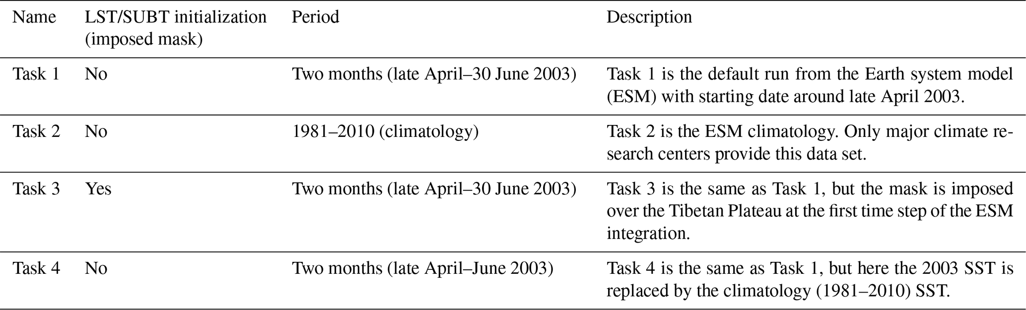
3.2.1 Task 1

In Task 1, each modeling group conducts a 2-month simulation starting from around late April to 1 May (e.g., 27, 28 April … 1 May, …) through 30 June 2003, consisting of a multi-member ensemble. Each group decides whether they use observed May and June 2003 SST and sea ice to specify the ocean surface conditions, which is similar to the AMIP (Atmospheric Model Intercomparison Project) experimental protocol, or use the specific ocean initial condition at the beginning of the model integration (for those ESMs which can run a fully coupled land–atmosphere–ocean configuration), similar to the CMIP (Coupled Model Intercomparison Project) experiment, or both. The reanalysis data are used as atmospheric and land initial conditions (as these ESM groups usually do). Since the spin-up time for different models for the S2S simulation varies, some groups start their simulations earlier than 1 May, for example, on 1 April or even earlier. LS4P does not require a specific number of ensemble members: each modeling group makes the decision based on their normal practice in performing their S2S simulations; however, it is required by LS4P that there should be no less than six members. The main purpose of Task 1 is to evaluate the performance of each model for the May 2003 T-2m and the June 2003 precipitation.

The evaluation of Task 1 results will be used to check (1) model biases in terms of the May 2003 T-2m across the Tibetan Plateau and in terms of June precipitation in the South and North Yangtze River basins (see the corresponding black/red boxes in Fig. 6b as a reference), (2) the lag relationship between these two biases, and (3) the model's ability to produce the observed May 2003 T-2m anomaly in the Tibetan Plateau and the June precipitation anomaly over the areas as listed in criterion (1). The CMA May 2003 T-2m and June 2003 precipitation, these two variables' climatologies, as well as topography data with a 0.5^∘ resolution (as discussed in Sect. 3.1) are used to calculate model biases, root-mean-square errors (RMSEs), and anomalies. When calculating the bias, it should be noted that the elevations of the T-2m observational data and model surface are usually not at the same levels, especially in high mountain regions. The observing stations tend to be situated in valleys and are generally at a lower elevation than the mean elevation of a model grid box. Before calculating the model bias, the model-simulated T-2m data must be adjusted with a proper lapse rate to the elevation height of the observational data as discussed in Xue et al. (1996a) and Gao et al. (2017).

The relationship between these two biases is evaluated to see whether they are consistent with the observed lag anomaly relationship, i.e., whether a cold/warm bias in May T-2m over the Tibetan Plateau is associated with a dry/wet bias in the southern Yangtze River basin and an opposite bias to the north of the Yangtze River basin. The consistency between these relationships would suggest the possibility that reducing the May T-2m bias may reduce the June precipitation bias if the observed May land surface temperature anomaly on the Tibetan Plateau does contribute to the observed June East Asian precipitation anomaly. In other words, if a model can produce the observed May T-2m anomaly, it may also be able to produce the observed June precipitation anomaly.

The discoveries from Task 1 will provide crucial information for the LS4P project to pursue its objectives as discussed in Sect. 2. If the LS4P ESMs produced no large bias in precipitation and T-2m and/or they were able to simulate the observed anomaly well over the Tibetan Plateau and eastern China, the justification for the LS4P approach would be questionable. Furthermore, should the model bias relationship between the May T-2m and the June precipitation be the opposite of the observed anomaly relationship of these two variables, it may be difficult to pursue the LS4P approach for these models. The preliminary assessments, however, are encouraging and strongly support the need for LS4P to further pursue its goals, and they will be briefly demonstrated in Sect. 5. It should be pointed out that the evaluation of the bias relationship between May T-2m in the Tibetan Plateau and June precipitation in eastern China is just a necessary condition for LS4P to pursue its approach, i.e., to propose a hypothesis. It is not sufficient to guarantee the model can improve the June precipitation prediction by using improved May T-2m initial conditions. Only Task 3, as discussed below, will serve this purpose.

3.2.2 Task 2

A number of LS4P modeling groups are from big climate modeling centers, and, as such, already have the required climatological runs in their respective databases. Those groups are required to send each year's global May T-2m and June precipitation from their climatological runs. Since different centers have different years in their climatology, LS4P only requires the climatological data set covering the time period from around 1981 to around 2010. The CMA precipitation and T-2m data averaged over 1981–2010 are employed to assess the simulated climatology biases and RMSE from these groups. The purpose of this task is to check whether the major bias features that we found in Task 1 based on year 2003 for the LS4P ESMs are also present in the modeled climatologies. Please note that discrepancies between simulated and observed fields are commonly referred to as biases, although differences for 2003 are not biases in the strict statistical sense, but for simplicity we use the term “bias” to refer to all these differences in this paper as done in Pan et al. (2001). Our premise is that the large biases in the high-elevation Tibetan Plateau region and in the East Asian drought/flood simulation produced by the LS4P ESMs are also persistent in the models' climatology. As such, any progress achieved in LS4P-I will not be limited to only 1 individual year, i.e., year 2003, but should have a broader implication. This issue will be further addressed in Sect. 5.

3.2.3 Task 3

Task 3 is the main LS4P experiment, which tests the effect of the May 2003 T-2m anomaly in the Tibetan Plateau on the June 2003 precipitation anomaly. Thus far, every ESM has a large bias in producing the observed May T-2m anomaly in the Tibetan Plateau, and so do the reanalysis data, which are used by the ESMs for atmospheric and surface initialization (see more discussion in Sect. 4.1). To reproduce the observed May T-2m anomaly in the Tibetan Plateau, which is the surface variable interacting with the atmosphere by influencing surface heat and momentum fluxes and affecting upwelling longwave radiation, initialization of the LST/SUBT has to be improved to generate the T-2m anomaly in the model simulation. Preliminary research within the LS4P modeling group suggests that prescribing both LST and SUBT initial anomalies based on the observed T-2m anomaly and model bias is the only way for the current ESMs to produce the observed May T-2m anomalies, unless the observed T-2m is specified during the entire model simulation, which would be a difficult task because, unlike specifying SST, LST has a large diurnal variation. It should also be pointed out that if we do not impose initial SUBT anomalies in a model simulation, the imposed initial LST anomaly and the corresponding T-2m anomaly would disappear after a couple of days of model integration. Studies based on observational data have shown a high correlation between LST and SUBT, and the memory in the soil subsurface is one of the major factors for producing soil surface temperature anomalies (Hu and Feng, 2004; Liu et al., 2020).

To improve the LST/SUBT initialization, a surface temperature mask for each grid point, ΔT_mask(i,j), over the Tibetan Plateau is produced based on each model bias and the observed climate anomaly. The (i,j) indexes represent the latitude and longitude coordinates of the grid point in the model. The initial surface temperature condition for Task 3 at each grid point after applying the mask, ${\stackrel{\mathrm{̃}}{T}}_{\mathrm{0}}\left(i,j\right)$, will be defined as follows.

Applying the mask, ${\stackrel{\mathrm{̃}}{T}}_{\mathrm{0}}\left(i,j\right)$, will be defined as follows:

$$\begin{array}{ll}{\displaystyle }& {\displaystyle }{\stackrel{\mathrm{̃}}{T}}_{\mathrm{0}}\left(i,j\right)=T_{\mathrm{0}}\left(i,j\right)+\mathrm{\Delta }{T}_{\mathrm{mask}}\left(i,j\right)=T_{\mathrm{0}}\left(i,j\right)\\ {\displaystyle }& {\displaystyle }+\left[-n\times T_{\text{obs anomaly}}\left(i,j\right)-T_{\text{bias}}\left(i,j\right)\right],\\ \text{(1a)}& {\displaystyle }& {\displaystyle }\text{when }{\overline{T}}_{\text{obs\hspace{0.17em} anomaly}}\times {\overline{T}}_{\mathrm{bias}}\ge \mathrm{0},{\displaystyle }& {\displaystyle }{\stackrel{\mathrm{̃}}{T}}_{\mathrm{0}}\left(i,j\right)=T_{\mathrm{0}}\left(i,j\right)+\mathrm{\Delta }{T}_{\mathrm{mask}}\left(i,j\right)=T_{\mathrm{0}}\left(i,j\right)\\ {\displaystyle }& {\displaystyle }+\left[n\times T_{\text{obs anomaly}}\left(i,j\right)-T_{\mathrm{bias}}\left(i,j\right)\right],\\ \text{(1b)}& {\displaystyle }& {\displaystyle }\text{when }{\overline{T}}_{\text{obs anomaly}}\times {\overline{T}}_{\mathrm{bias}}<\mathrm{0},\end{array}$$

where T₀(i,j), T_bias(i,j), and T_{obs anomaly}(i,j) correspond to the original model surface initial condition (used in Task 1), monthly mean model bias, and monthly mean observed anomaly, respectively, at grid point (i,j), where n is a tuning parameter which is described in a subsequent paragraph. Please note that there are no observed daily land surface temperature data available over the globe. The ${\overline{T}}_{\text{obs anomaly}}$ and ${\overline{T}}_{\mathrm{bias}}$ are the averaged observed anomaly and model bias, respectively, over the entire area where the mask is intended to be applied, such as the Tibetan Plateau. Equation (1a) is applied for the situation when observed anomaly and model bias have the same sign, while Eq. (1b) is used when observed anomaly and model bias have different signs, regardless of whether the anomaly is positive or negative. Figure 2 shows schematic diagrams for imposed masks for surface temperature initialization under different conditions, which delineates the concept for the mask formulation. In this figure, a cold year (such as year 2003 that is used in the LS4P Phase I) is selected for demonstration. A schematic diagram, also based on Eq. (1), for the warm year (such as year 1998) was displayed in Supplement Fig. S1 as a reference for readers in order to help them to organize their own experiments with different scenarios.

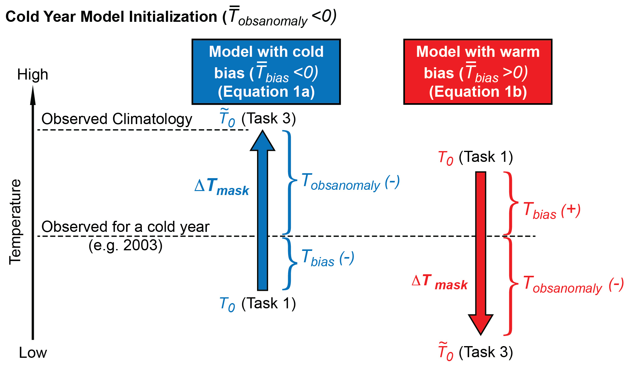
Figure 2 Schematic diagram for an imposed mask for surface temperature initialization in Task 3 corresponding to a cold anomaly year. Notes. (1) The part with blue/red color has bias and anomaly over the area with the same/different signs, respectively. (2) The ± sign in the parentheses indicates that the value is positive/negative, respectively. The notation “= T_{obs anomaly} (–)” indicates that it has the same value as the observed negative anomaly. (3) For simplicity, Fig. 2 is only for the grid points in which a sign of the bias is the same as the sign of area-averaged bias. (4) T₀ is the initial condition for Task 1, and ${\stackrel{\mathrm{̃}}{T}}_{\mathrm{0}}$ is the initial condition after imposing the mask for Task 3.

In Eq. (1), we use ${\overline{T}}_{\text{obs anomaly}}$ and ${\overline{T}}_{\mathrm{bias}}$ to determine whether Eq. (1a) or (1b) is employed, because even if a model has a general strong warm/cold bias for the entire area, there are always a few grid points where the bias is reversed. For anomalies, we did not find individual grid point and area average having different signs since we always select areas and seasons with relatively large T-2m anomalies (Fig. 1). Using ${\overline{T}}_{\mathrm{bias}}$ as a criterion in Eq. (1) will prevent the initial conditions of those grid points from adjusting in an opposite direction from the majority of other grid points. In other words, if most grid points in Task 3 have higher/lower initial surface temperature than that in Task 1, so do these grid points (with opposite bias) after imposing the mask. For simplicity, these scenarios are not displayed in Fig. 2.

Figure 2 along with Eq. (1) delineate how the grid points' initial conditions in Task 3 are adjusted. The methodology presented here is to create the initial condition ${\stackrel{\mathrm{̃}}{T}}_{\mathrm{0}}\left(i,j\right)$ for Task 3 and to produce the observed LST anomaly with the difference between Task 3 and Task 1. One of the LS4P Phase I goals is to examine how such an anomaly affects the summer downstream precipitation S2S predictability. For some ESMs, it may not produce the optimal initial condition if they choose observed climatology, not Task 1, as their reference. However, with the understanding gained from this experiment plus a slight modification of Eq. (1), this approach should also serve this purpose. It needs to be pointed out that ${\overline{T}}_{\mathrm{bias}}$ in some cases may not be available. In Sect. 5, we will show that ${\overline{T}}_{\mathrm{bias}}$ for a model's climatology and for a specific year generally are quite consistent, so the climatological bias can be applied if there is no better information. As discussed earlier, the sign of the bias is crucial to determine how to make the mask.

Because all the models are unable to maintain the soil temperature anomaly (or produce adequate soil memory), a tuning parameter “n” (e.g., 1, 2, or 3) is introduced. Through trial and error, each model selects a proper “n” with the intention of producing the T-2m anomaly which is close to observation. For the subsurface, the “n” may be different from that for LST depending on the ESM's land surface scheme. However, currently, most modeling groups use the same “n” for every soil layer. Better initialization for soil sublayers can be improved after more deep-soil-layer measurements are available.

Figure 3 shows a mask application example from one LS4P model, which has a warm bias (Fig. 3b). Based on the bias and the observed May 2003 T-2m anomaly, a mask using Eq. (1b) (given the model has warm bias) was generated and only imposed over the Tibetan Plateau region as demonstrated in the global map (see Fig. 3c). The mask is imposed on the initial condition at the first time step of the model integration. The model run starts around 1 May and runs through 30 June with multi-ensemble members (the same total number as for Task 1), and the LST/SUBT is updated by the ESM after the initial imposition of the mask. However, in the example shown in Fig. 3, the mask using n=1 failed to produce a proper May T-2m anomaly (Fig. 3d). Once the model produces a reasonable observed May T-2m anomaly through a tuning of “n” in Eq. (1) (in Fig. 3, only the mask with n=3 produces a proper May T-2m anomaly), the June precipitation difference between the Task 3 run and the Task 1 run is then evaluated.

Figure 3 Schematic diagram for the mask application. (a) Obs. May 2003 T-2m anomaly over the Tibetan Plateau (TP), (b) May 2003 T-2m simulation bias over the TP from a LS4P model, (c) imposed mask with n=1 for a LS4P model, (d) simulated May 2003 T-2m anomaly over the TP after imposing the mask shown in (c), (e) as in (c) but with n=3 (only the TP is displayed here), and (f) as in (d) but with n=3.

To assess the model simulation in this task, we produce composite data sets for global May and June T-2m and precipitation for both the year of 2003 and climatology, in which the CMA data are used within China for both variables (Han et al., 2019; X. Liang et al., 2020), while Climate Anomaly Monitory System (CAMS, Fan and Van den Dool, 2008) and Climate Research Unit (CRU, Harris et al., 2014) data are used elsewhere for T-2m and precipitation, respectively. These composite data are used to evaluate whether the May T-2m difference between the Task 3 run and the Task 1 run produces the observed May T-2m anomaly over the Tibetan Plateau, which is the key objective of Task 3. If a model can produce about 25 % of the observed May T-2m anomaly over the Tibetan Plateau, we will further examine the difference of the June global precipitation between the two runs and observed global June precipitation anomaly. Moreover, the improvement in reducing the bias and RMSE for the sensitivity runs will also be assessed.

3.2.4 Task 4

Task 4 tests the effect of the ocean state on the June 2003 precipitation. There are two possible approaches for this test. Groups with the AMIP type of experiment use the observed May and June 2003 SST for their Task 1 and Task 3 experiments. For those groups, in Task 4, the 2003 SST conditions will be replaced by the climatological SST. For modeling groups using the CMIP-type experimental setup, the 2003 initial condition used in Task 1 and Task 3 will be replaced by the climatological initial condition. The year 2003 is a La Niña year. The modeling groups with the CMIP type of simulation need to check their models' SST simulations to be sure that their models are producing adequate La Niña conditions along the western coast of South America and the eastern Pacific. The June precipitation difference between the control run (with the 2003 ocean state) and the Task 4 run (with the climatological ocean state) will be compared with the observed anomaly in 2003 to assess the global ocean state effect on the precipitation; then, it will be compared with the LST/SUBT effect from the Task 3 results. These four tasks are summarized in Table 1.

4 Model output and availability

The data output requirements take into account the evaluations that are required as discussed in Sect. 3.2.1–3.2.4 along with the information required to characterize the land surface–atmosphere interactions at and near the surface and the mid- and upper-troposphere atmospheric wave propagation. In addition to the T-2m and precipitation, other model outputs from the land surface and the atmosphere (Table S1 in the Supplement) will also be used to evaluate the model results. The NOAA metrics and protocol for short- to medium-range weather forecast performance evaluations as discussed in Wang et al. (2010) will be applied to assess model performance. Careful considerations are necessary to limit output frequency in order to save storage while still providing sufficient information for crucial diagnostic analyses. The LS4P data are stored and will be distributed through the National Tibetan Plateau Data Center (Li et al., 2020) and the U.S. Department of Energy Lawrence Livermore National Laboratory Earth System Grid Federation (ESGF) node (Cinquini et al., 2014). The detailed information is described in Appendix C.

5 Main issues in LST/SUBT initialization and deficiency in model memory

To date, all the LS4P ESMs with their land models have difficulty producing the observed T-2m anomaly over the Tibetan Plateau to varying degrees. Moreover, they are also unable to maintain the imposed LST/SUBT anomaly from the mask during the model integration. The current model deficiencies in T-2m simulation are rooted in the data, mainly from the reanalysis data, which are used for the model initialization, and the model parameterizations. Certain studies (Liu et al., 2020; Li et al., 2021) have identified the roles of land parameterizations and soil depth related to this deficiency. More research is necessary to further elucidate the potential roles of other ESM parameterizations. The LS4P has developed an initialization scheme which seeks to mitigate this deficiency in order to yield better S2S prediction. Further development is necessary to improve this approach. Eventually, the model's deficiencies in producing observed high mountain surface temperature anomalies should be overcome through the development of proper physical and dynamic processes and relevant data sets to preserve land memory, which is a long-term task and requires community efforts. This section will discuss a few relevant issues based on our practice, intending to raise the community's interest and attention and to promote more comprehensive developments in this aspect.

5.1 Data uncertainty

Observational T-2m/LST/SUBT data are crucial for model initialization of surface conditions and for model validation. However, ground measurements over high-elevation areas are relatively sparse. For instance, most currently available gridded global T-2m data sets with long records only consist of a few dozen stations over the Tibetan Plateau. Considering the complex topography of the region, potentially large interpolation errors can occur. The same is true for the reanalysis data, which are used for the model initialization. In most reanalysis data sets, the T-2m is only a model product. In LS4P, we employ the CMA T-2m data (1980–2017) with a 0.5^∘ resolution (Han et al., 2019; X. Liang et al., 2020) for model initialization, which is based on about 150 ground station measurements over the Tibetan Plateau. Figure 4 shows the May T-2m climatology (the 1980–2013 average) over the Tibetan Plateau and the anomalies of May 2003/1998, which correspond to a very cold/warm spring in the Tibetan Plateau, respectively, from CMA, CAMS, CRU, Climate Forecast System Reanalysis (CFSR, Saha et al., 2014), ERA-Interim (ERAI, Berrisford et al., 2011), and the Modern-Era Retrospective analysis for Research and Applications, version 2 (MERRA-2, Gelaro et al., 2017). Because each T-2m data set has its own elevation, all the data have been adjusted to the CMA elevation for comparison. Compared with the CMA data, the CAMS/CRU climatology is about 1.8 ^∘C cooler/1.5 ^∘C warmer, respectively. The biases for warm/cold years are even larger for CAMS/CRU (not shown), respectively. While the climatological bias for CFSR data is small, the bias for ERAI is still on the order of 1 standard deviation of the Tibetan Plateau T-2m variability (∼ 0.7 ^∘C). The bias is larger in MERRA-2, at about 4 ^∘C. In addition, for cold/warm years, MERRA-2 and CFSR show opposite anomalies. The large surface temperature biases in the reanalysis data sets likely interact with temperature of the lower atmosphere. There are limited atmospheric sounding data over the Tibetan Plateau for data assimilation. That said, lower atmosphere temperature is also subject to model bias. Since there are no observed near-surface-layer observations, we compare the reanalysis-based surface and near-surface temperature anomalies with their own climatology. These anomalies are very close (not shown), which means that even if we impose a mask to overcome the LST/SUBT bias, the bias in the lower troposphere is still there. This bias in the reanalysis data has an important implication in affecting the LST initialization and its simulation, which will be discussed further in Sect. 4.2.

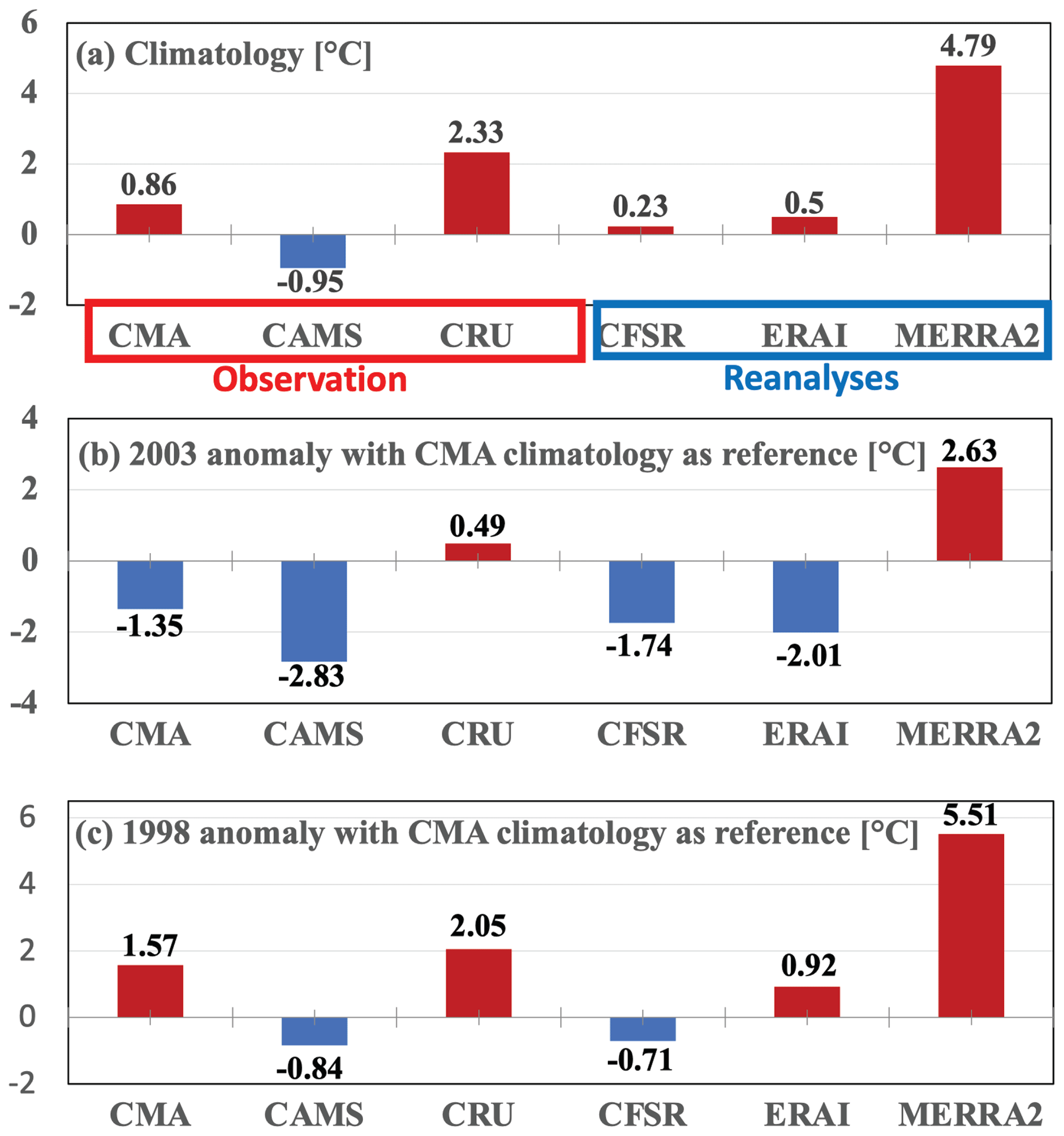
Figure 4 May T-2m over the Tibetan Plateau above 4000 m from observational and reanalysis data sets; (a) mean climatology, (b) 2003 anomaly (a cold May) and (c) 1998 anomaly (a warm May). Note. The CMA climatology is used as a reference for the anomalies. Because each T-2m data set has its own elevation, all the data have been adjusted to the CMA elevation for comparison.

In addition to the surface temperature, subsurface temperature initialization is also challenging in high-elevation areas. Measurements for deep subsurface conditions do not exist in most mountain areas. However, there are 14 stations in the Tibetan Plateau (Fig. 5a) that have soil temperature measurements during the period 1981–2005 at depths of 0, 5, 10, 15, 20, 40, 80, 160, and 320 cm, which shed light on the quality of subsurface-layer temperature in the reanalysis data. Below 320 cm, the soil temperature exhibits very little annual variation. The soil temperature profiles from station observations are averaged, and 4 typical months that represent the four seasons are displayed in Fig. 5b. The differences between the T-2m and the LST are less than 1^∘ for these 4 months. During winter and summer, the deep soil temperature profiles show a larger lag compared with the LST. The reanalysis products over the grid points closest to the observation stations (Fig. 5a) have been averaged over the same time period. However, these data show large discrepancies compared with observations in addition to biases (Fig. 5b–c). For instance, the top 1 m soil temperatures in the ERAI data are nearly constant for every season, with little change with soil depth. In MERRA-2, the lag response in the soil profiles only appears in the winter and summer up to about 1 m deep; for other seasons or soil temperatures below 1 m this does not change much. The CFSR shows a better lag response, but it only reaches 1.5 m in depth. Its biases in these stations compared with the observation stations are also apparent.

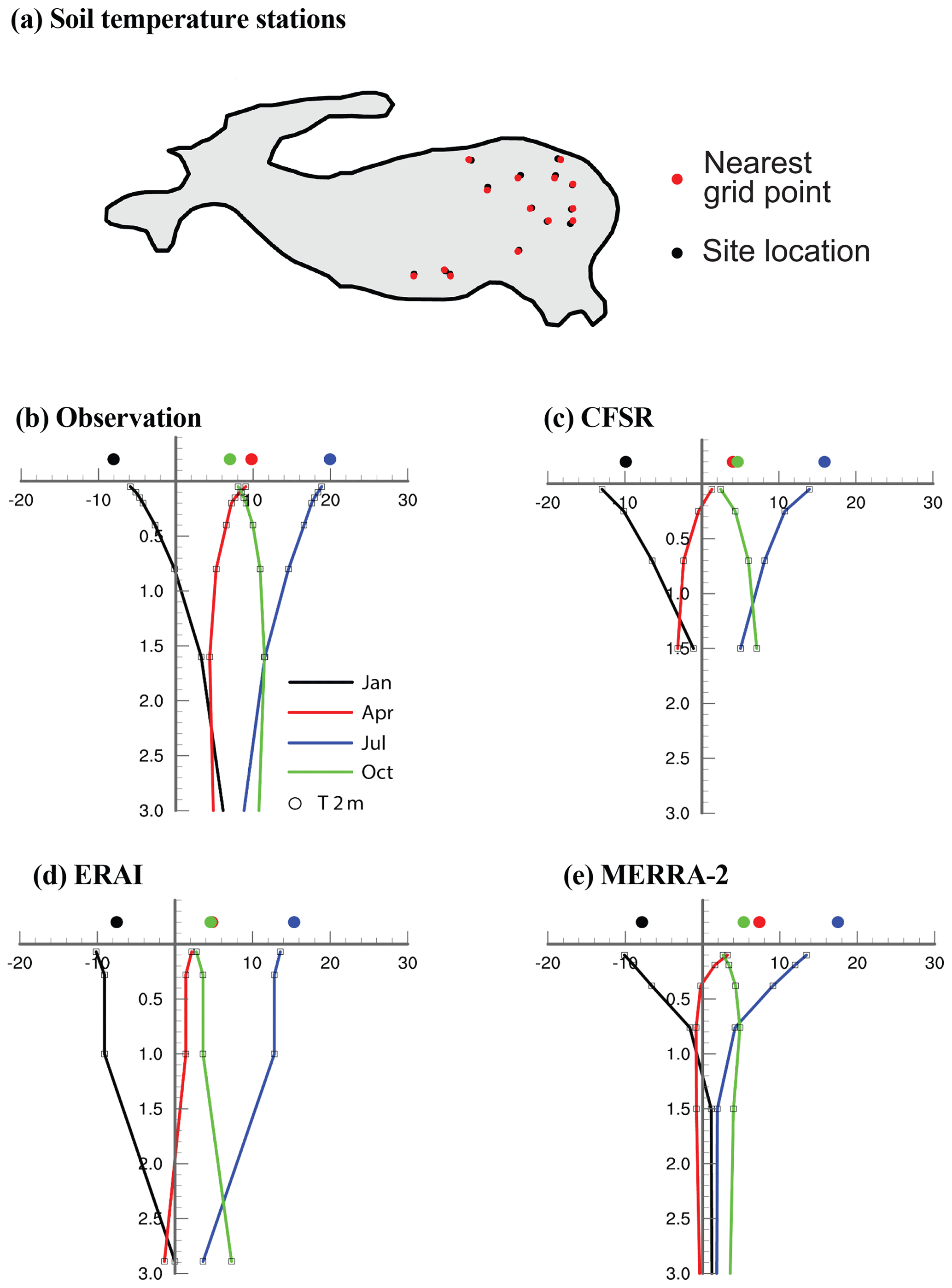
Figure 5 Mean soil temperature profiles in different seasons based on 14 TP stations and compared with different reanalyses.

The deficiencies in the reanalysis products pose a challenge for properly producing the observed T-2m anomalies since the reanalyses are used to provide the basis for the surface initial condition for most ESMs. Since every LS4P ESM showed a large bias in simulating the May 2003 T-2m anomaly over the Tibetan Plateau, we have addressed how to take the bias into account in producing the initial condition mask in Sect. 3.2. In the next section, the efforts from different modeling groups to generate the observed T-2m anomaly are presented further.

5.2 Approaches to improving the LST/SUBT initialization and T-2m anomaly simulation

In addition to the data that are used for LST/SUBT initial conditions, land models also have deficiencies in maintaining the anomalies that are imposed using an initial mask as discussed in Sect. 3.2. In the LS4P-I experiment, most models are only able to partially produce the observed T-2m anomaly in May despite the imposed initial masks. The recent available daily Tibetan Plateau surface data from the LS4P data group show our imposed initial anomaly is not extreme, but models lost the imposed anomaly rather quickly. This section highlights some specific approaches undertaken by a few groups during their application of the LS4P-I protocol to improve the T-2m anomaly simulation.

The surface soil (20–30 cm) in the central and eastern Tibetan Plateau contains a large amount of organic matter which greatly reduces the soil thermal conductivity and increases the soil heat capacity (Chen et al., 2012; Liu et al., 2020). However, this factor is not taken into account in the LS4P ESMs, except for CNRM-CM6-1. That said, the soil thermal conductivity/heat capacity over the Tibetan Plateau in the ESMs is too high/too low. In addition, some ESMs overestimate the precipitation over the Tibetan Plateau, making the soil water content higher than in reality (Su et al., 2013), which also leads to higher soil thermal conductivity. Less soil organic matter and high soil moisture both accelerate the heat exchange rate between the soil and the atmosphere, which causes the rapid loss of soil thermal anomalies in the models.

The soil-layer depth in the ESM also affects the model's ability to generate the observed T-2m anomaly. The long memory in deeper soil helps to preserve the soil temperature anomaly in shallower layers. In a sensitivity study that changed the soil depth from 6 to 3 m, it was found that with reduced total soil column depth, a similar magnitude anomalous soil temperature can only be kept for about 20 d, and then it disappears much more quickly compared with the 6 m soil-layer model (Liu et al., 2020). The total soil column depth may not be deep enough in some LS4P models. To overcome these shortcomings in current ESMs and to reproduce the observed T-2m anomaly, a tuning parameter “n” is introduced (Eq. 1) when setting up the surface mask since it is not a simple task to increase the soil-layer depth for all the ESMs.

One of the intentions of the initialization of LST/SUBT is to influence the lower atmosphere since the corresponding initial condition from reanalysis also has inherent errors as discussed in Sect. 5.1, and for some models they can be quite large. A number of modeling groups have started the model simulation earlier, for instance, on 1 April, in order to have sufficient time for the lower atmosphere to spin up and to be consistent with the within-mask imposed soil surface conditions. In some models, such as ACCESS-S2 and KIM, the models make an adjustment after reading in the initial condition, usually referred to as shock adjustment, in order to avoid an imbalance between the atmosphere, land, and ocean initial conditions. This shock adjustment has become a more popular practice in a number of modeling groups. The idea behind the shock adjustment arises from the potential inconsistency among different sources of initial conditions and the belief that the atmospheric components are considered to be relatively the most reliable. With such an approach, within the first week or 10 d, the atmospheric forcing plays a dominant role in adjusting the other components' initial conditions. As such, the imposed initial soil temperature from the mask at the top soil layers could be compromised very dramatically toward the lower atmospheric conditions, which, unfortunately, also have large errors over the Tibetan Plateau as previously discussed. Although the imposed deep soil temperatures eventually start to affect the air temperature, this process generally takes more than 20 d. For the model with such a shock adjustment, the mask needs to be imposed when the shock adjustment becomes weak, such as at the second day in ACCESS-S2 or half a month after the initial simulation date, as done in KIM. As such, the models may have to start their integrations much earlier. A couple of models tried to impose the mask more than once to produce the T-2m anomaly. For instance, the FGOALS-f2 model imposed the LST/SUBT anomaly on both 1 and 2 May to better produce the observed T-2m anomalies. It should be pointed out that if a mask is imposed too many times, the ΔT in the mask may add up every time when it is imposed to become quite a large sink/heat source. Furthermore, enforcing the LST/SUBT perturbation too many times during the model simulation with accumulated large ΔT may distort the atmospheric conditions. Precautions must be taken in this type of approach, probably with ΔT imposed no more than twice with a well-designed scheme to avoid the excessive accumulation of heating/cooling.

For the E3SM and CESM2, which are mainly used in long-term climate research (e.g., century-long simulations), real-time initialization for S2S prediction is not very closely related to the research objective the model centers intend to pursue. To conduct LS4P-type research, the modeling groups have to develop an approach in nudging the reanalysis data for a real-time initialization. Nudging is one of the simplest data assimilation methods (Hoke and Anthes, 1976) and has been widely used in climate model evaluation and sensitivity studies (e.g., Xie et al., 2008; Sun et al., 2019; Tang et al., 2019) to constrain the simulations towards a predefined reference (the reanalysis data in this case) and hence to facilitate time-specific comparisons between model and observations. For the LS4P simulations, E3SM and CESM2 used 1 month worth of nudging of the horizontal wind components (U and V) with a 6 h relaxation timescale before the land mask for the initial LST perturbation was applied. A study (Ma et al., 2015) has shown that nudging only horizontal winds produces better results compared with those with nudging of more variables, such as temperature or specific humidity.

6 Discussion: perspectives and impact of LS4P

LS4P is the first international grass-roots effort focused on introducing spring LST/SUBT anomalies over high mountain areas as a factor to improve S2S precipitation prediction through the remote effects of land–atmosphere interactions. Although the original idea of starting LS4P was more limited and only aimed at evaluating whether the results from preliminary tests with one ESM and one RCM (Xue et al., 2016b, 2018) could be reproduced by more modeling groups, multi-model participation has quickly led to the recognition that the Tibetan Plateau's spring LST/SUBT effect on the precipitation anomaly to the south and north of the Yangtze River was only a small part of broader aspects.

Figure 6 shows the observed May T-2m and June precipitation anomalies in 2003 and the corresponding ensemble mean biases from 13 LS4P ESMs for these two variables in 2003 over the eastern part of Asia. As discussed in Sect. 3.2.1, the appropriate relationships between model biases and observed anomalies are crucial for the LS4P hypothesis and approach. Among the 13 ESMs, 11 ESMs had warm T-2m biases, while the remaining 2 had cold biases, respectively. Because the May 2003 T-2m had a cold anomaly, the T-2m and precipitation biases for the models with positive T-2m bias were multiplied by −1 to produce the ensemble mean composites as shown in Fig. 6c and d. We note the caveat that the ESM results are from ensemble means, and in comparing with a particular year the spread of the ensemble results is also important. However, one can immediately see that the biases are substantial, despite the particular combination of ESM results indexed to the Tibetan Plateau temperature. Despite ESM results being produced from models with different numerical approaches and physical parameterizations, the modeled bias relationships between May T-2m and June precipitation are very consistent with the observed anomaly relationship between observed May 2003 T-2m over the Tibetan Plateau and June 2003 precipitation in many parts of eastern Asia, in addition to the Yangtze River basin. For instance, models with a cold bias in May T-2m in the Tibetan Plateau also have a dry bias in June precipitation over northeastern Asia, part of Southeast and South Asia, and Siberia and a wet bias to the west of Siberia, consistent with the observed precipitation anomaly. The spatial correlations between observed June precipitation anomalies and the corresponding model biases over the figure domain are 0.62. Furthermore, the T-2m cold bias over the Tibetan Plateau is associated with a cold bias in the Iranian highlands and a warm–cold–warm wave train over the Eurasian continent, which is also generally consistent with the observed T-2m anomalies. Moreover, the consistencies suggest a possibly much larger-scale remote effect of the Tibetan Plateau LST/SUBT on summer precipitation over many parts of the world and support the LS4P's approach in its experimental design as discussed in Sect. 3.2. As a result, the diagnostic analyses from the tasks in Experiment 1 will cover the entire globe. Comprehensive analyses and discussion will be presented in subsequent papers after the LS4P groups have completed their experiments.

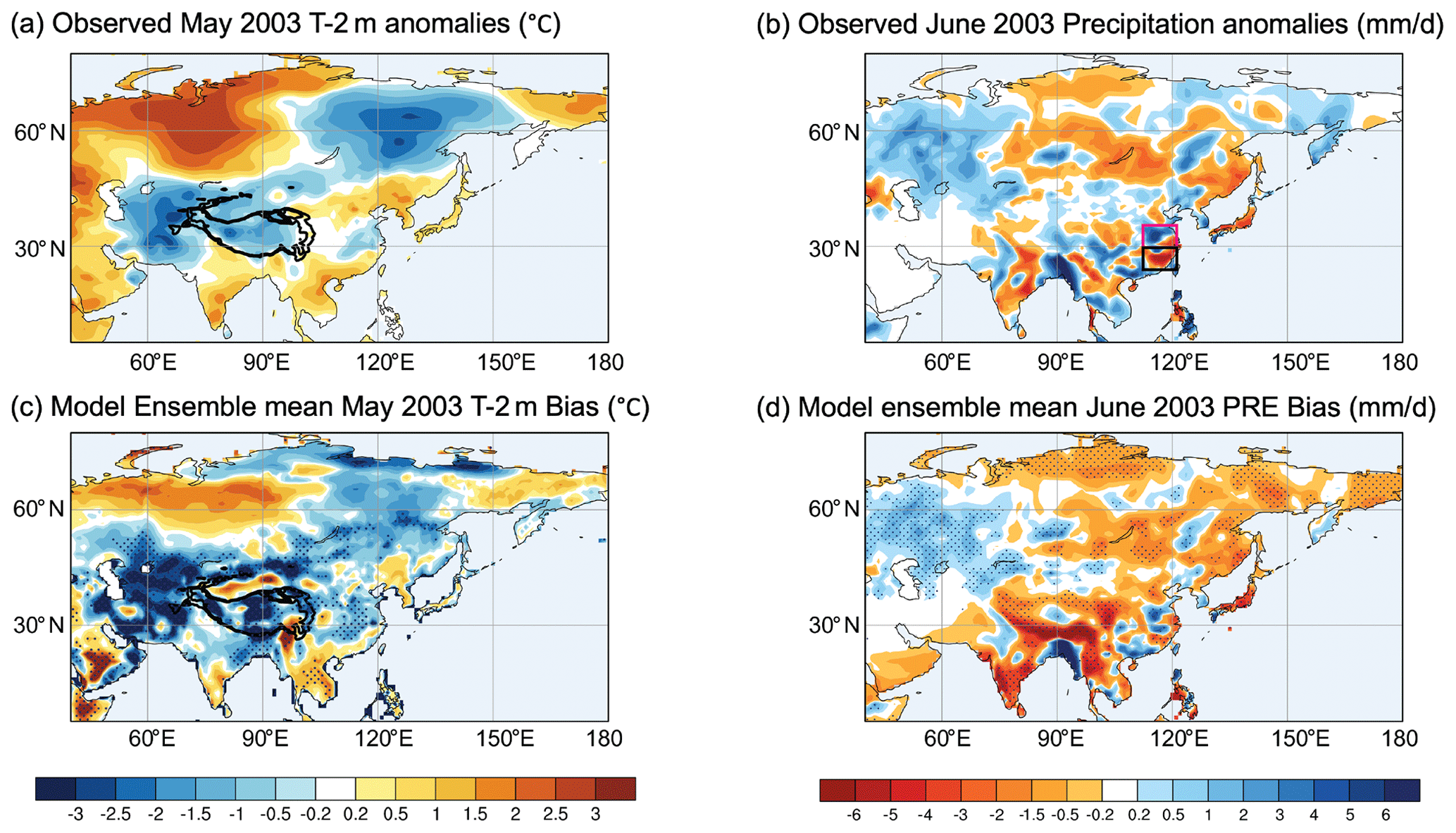
Figure 6 Comparison between the observed anomalies and the ensemble mean bias for May 2003 from 13 LS4P-I Earth system models (ESMs).

Although the T-2m anomaly covers large areas, our previous North American study has shown that only the LST/SUBT anomaly over high mountains (the Rockies) had a substantial impact on the subsequent drought over the South Great Plains (Xue et al., 2012). One of the LS4P groups, KIM, also tested the effect of the LST anomaly in other parts of East Asia but found their effects are incompatible with the Tibetan Plateau LST/SUBT effect. In addition to the year 2003, we also checked the May T-2m and June precipitation bias in the climatologies of the different models. The 13 ESMs shown in Fig. 6 have also provided their climatological data sets. Figure 7 shows the climatological biases for May T-2m and June precipitation from these ESMs. The patterns between the bias in the 2003 simulation and the bias in the model climatologies are generally consistent, which is important, because the climatological bias is substantial and affects the individual years as well. In Phase I, through the LS4P RCM efforts in incorporating the TPE and TIPEX-III data, we also intend to simulate the water and energy cycle and atmospheric conditions in the Tibetan Plateau and their variability. These simulations will provide the data for better atmospheric and surface initialization along with obtaining an improved understanding of the atmospheric circulation and water cycle in the “Tibetan Water Tower”.

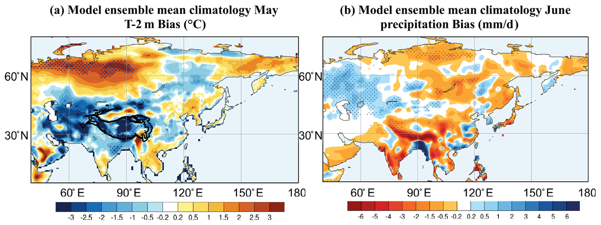
Figure 7 Thirteen LS4P-I ESM ensemble mean climatology biases.

Thus far, the discussion has been focused on the modeling approach. A recent statistical study has shown that spring soil temperature in central Asia could be a predictor of summer heat waves over northwestern China (Yang et al., 2019). In addition, surface temperatures from five northern European observing stations have been used as predictors for long-range forecasting of monsoon rainfall over southwestern India (Rajeevan et al., 2007). Moreover, spring (April–May) precipitation and 2 m air temperature over northwestern India, Pakistan, Afghanistan, and Iran have been found to have a strong link to the first phase (June–July) of summer monsoon rainfall over India (Rai et al., 2015). We will extend the data analyses for different major mountains and different seasons and identify hot spots over the globe where LST has significant impacts. Preliminary statistical forecasts will also be explored, using methods such as canonical-correlation analysis (CCA) and joint empirical orthogonal analysis (JEOF) (Smith et al., 2016). Based on the statistical analyses, a Tibetan Plateau oscillation index (TPO) and a Rocky Mountain oscillation index (RMO) will be proposed for predictions of the hydroclimatic extreme events, and a relationship between the TPO and RMO indexes will also be investigated. As discussed in Sect. 3, the Rocky Mountain LST/SUBT effect will be the focus of LS4P Phase II (LS4P-II).

The LS4P research has revealed some severe deficiencies in current land models in preserving the land memory. In many models, the force-restore method (Deardorff, 1978; Dickinson, 1988; Xue et al., 1996b) is used to represent subsurface heat transfer and soil thermal status. This simple method produces adequate diurnal and seasonal cycles of surface temperature and thus has been widely used by many land models for decades. However, its severe deficiency in keeping the soil memory is apparent in recent studies (Liu et al., 2020; Li et al., 2021). We have found that excessively shallow soil depths along with simplified parameterizations of subsurface heat transfer are acting to limit the soil memory effect in many models, especially in cold regions. An innovative approach has been developed for the land model initialization that can help maintain the monthly LST/SUBT anomaly. The LS4P's finding on why ESMs have difficulty in maintaining the LST anomaly, and its proposed approach to help solve the issue should be a significant contribution from the LS4P project to improve the S2S prediction. We also hope to have more studies to explore the causes of this deficiency from different aspects further.

LS4P focuses on process understanding and predictability. Since the current start-of-the-art models are unable to properly produce the observed surface temperature anomaly and the corresponding anomaly-induced dynamic as well as the associated physical processes in their simulations, the bias correction in post-processing (a method that has been used for some simulation studies) is unable to generate these processes to help our understanding and will not be considered in the LS4P project. However, we encourage/welcome different approaches to tackle this issue and for comparison with the approach presented in this study.

One issue that hampers the application of the LST/SUBT approach for S2S prediction is data availability. The TPE has conducted comprehensive measurements over the high mountain Tibetan Plateau areas, which include a plateau-scale observation network plus intensive networks at more local scales: these data consist of boundary-layer observations and land surface and deep-soil-layer measurements. These measurements have provided invaluable information to support the establishment of the LS4P and to foster further model development and the possible causes of land memory. Currently, such comprehensive measurements over high mountain areas are still lacking across the globe. GEWEX has been planning for more measurements that are related to land–atmosphere interactions (Boone et al., 2019; Wulfmeyer et al., 2020; Schneider and van Oevelen, 2020). We hope that the results from LS4P will demonstrate the substantial role of high mountain surface conditions in global climate and atmospheric circulation and therefore stimulate more initiatives to increase land–atmosphere interaction measurements over high mountain regions.

LS4P will complete the Phase I tasks at the end of 2020. A special issue in Climate Dynamics was initiated in late 2020 to report various LS4P research results and other S2S prediction research results that should help increase the understanding and predictions of land-induced forcing and atmosphere interactions on droughts/floods and heat waves. We plan to kick off the LS4P-II in the summer of or later in 2021 with a workshop at the Earth System Science Interdisciplinary Center (ESSIC), University of Maryland, College Park, USA. This workshop will summarize the Phase I activity and design working tasks for the LS4P-II. Phase I focuses on the case of 2003. In the ensuing LS4P activity, more cases will be tackled, which will further improve our assessment of the ESM's predictability linked to LST/SUBT. Although the land has a lower heat capacity and less moisture compared with the oceans, the land surface has a much stronger response to changes in surface net radiation at diurnal, subseasonal, and seasonal scales compared with oceans. This is particularly true in high-elevation areas, which could provide a useful source of predictability at these scales. LS4P intends to improve the S2S precipitation prediction through a better representation of land surface processes in the current generation of ESMs and aims to make a fundamental contribution to advancing S2S prediction through proper initialization of LST/SUBT in high mountain regions. The LS4P approach proposes a new front in S2S prediction to complement other existing approaches. We hope activities and results from LS4P-I can provide a prototype approach to raise further scientific questions and open a new gateway for more studies with various approaches to better understand the roles of different forcing and internal dynamics in S2S predictability along with identifying the relevant mechanisms.

Appendix A: List of LS4P-I Earth system models (ESMs) and regional climate models (RCMs)

Table A1 List of LS4P-I Earth system models.

Table A2 List of LS4P-I regional climate models.

Appendix B

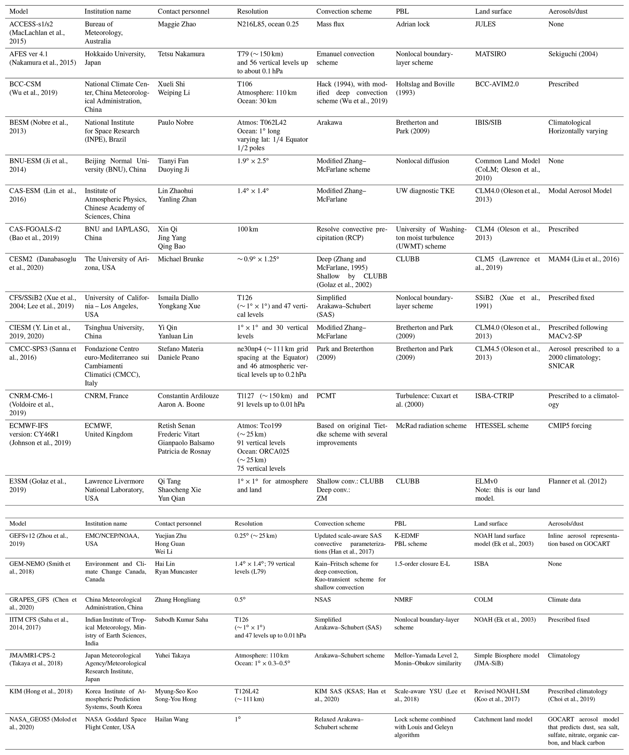
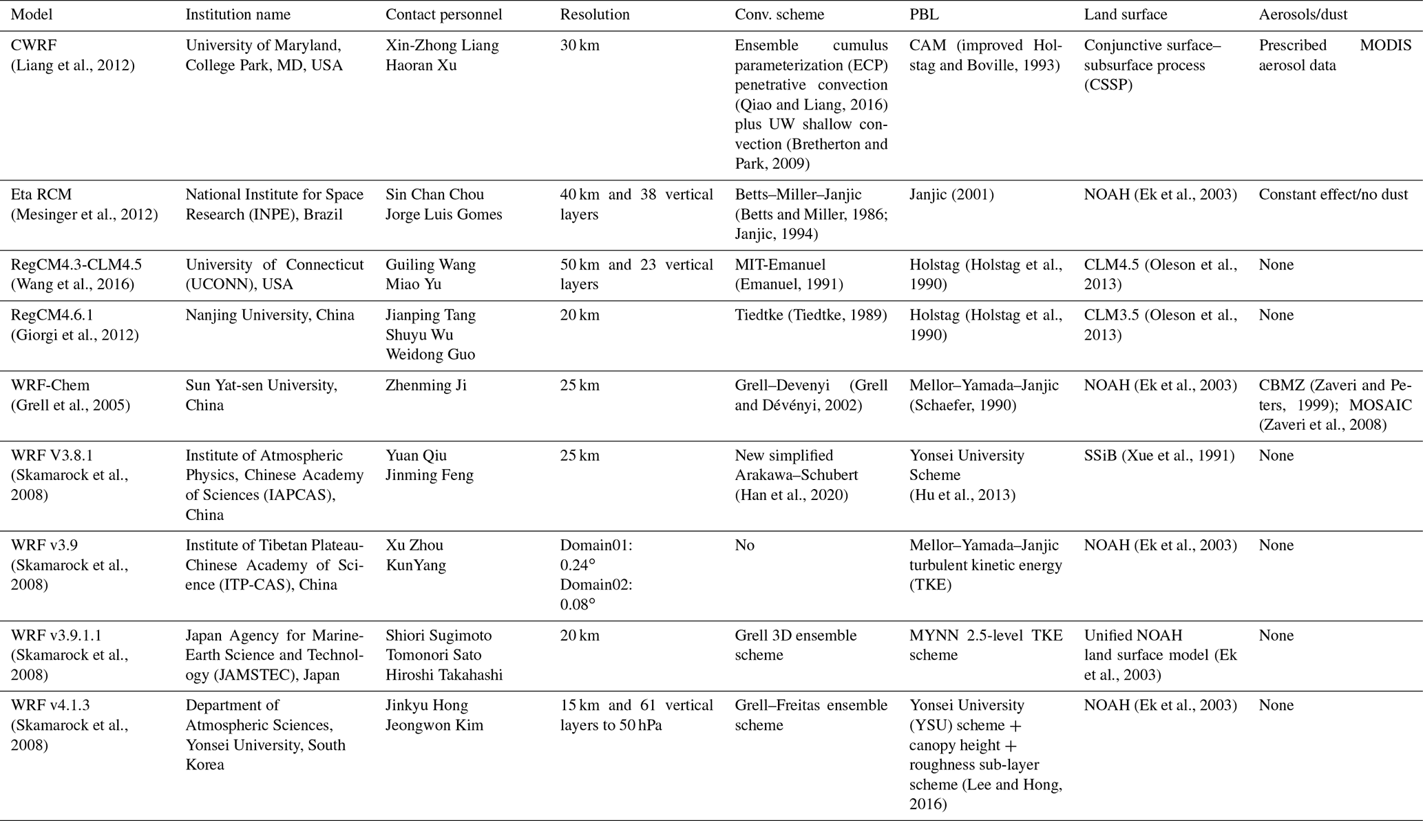
Table B1 List of observations and reanalyses used in the LS4P Phase I study.

Appendix C: Model output and availability

Five types of variables are requested: they include monthly and daily mean three-dimensional atmospheric profile variables at 1000, 925, 850, 700, 600, 500, 300, 200, and 100 hPa as well as monthly, daily, and 6-hourly/3-hourly two-dimensional surface variables. The detailed variable requirements are listed in Supplement Table S1. Since LS4P-I explores the timescales necessary for realistic simulation of subseasonal and seasonal (S2S) weather and climate phenomena, a minimum amount of sub-daily data is required to allow the diagnosis of phenomena related to S2S and monsoon systems. These model outputs are generally consistent with the requirements of the NOAA metrics and protocol for short- to medium-range weather forecast performance evaluations. If a model does not output one of the requested variables, it should report it as a missing value. Due to the nature of the LS4P project, daily surface temperature and precipitation data must be included, especially surface temperature data, which will be used to check and improve the model performance with respect to its ability to reproduce the observed T-2m anomaly. Finally, only ensemble means are required.

The LS4P data are stored and will be distributed through the National Tibetan Plateau Data Center (http://data.tpdc.ac.cn/en/, last access: 1 June 2021) and the U.S. Department of Energy Lawrence Livermore National Laboratory Earth System Grid Federation (ESGF) node (https://esgf-node.llnl.gov/projects/esgf-llnl, last access: 1 June 2021). The National Tibetan Plateau Data Center has an online data submission system similar to that used for paper submission. For instance, folders can be uploaded without being tarred into a single file. It is also recommended that each modeling group create its own folder, which may contain many subfolders/files, using labels such as Task1 or Task2, under which it is suggested to create more subfolders for the monthly, daily, and 6-hourly data, respectively.

Data files must comply with the NetCDF format version 4. The names of the files in the LS4P archives should follow the example below and must appear in the following order: VariableName_LS4P_ESMModelName_ LS4PExperimentName_Frequency_[StartTime-End Time].nc. For example, the file name, pr_LS4P_UCLACFSSSiB2_Task1_6hr_00z01052003-18z30062003.nc, represents the precipitation data from Task1 using the UCLA CFS/SSiB2 model and covers the period from 1 May through 30 June 2003 (i.e., the date is recorded as ddmmyyyy). A document that specifies the technical aspects of LS4P data archive and data formats, including the common naming system, is provided in Appendix D.

Appendix D: LS4P-I data archive design

This Appendix specifies technical aspects of the LS4P-I data archive and data formats, including the common naming system. The list of requested LS4P-I variables and timescales is contained in “LS4P_ESM_outputs_list_update” available from https://ls4p.geog.ucla.edu/experiments/ (last access: 1 June 2021), but it could also be directly downloaded from the following link: https://ucla.box.com/s/oeo8yq9jx58im4mlfd5lgbnl42ewk180 (last access: 1 June 2021).

• I.

  File format and file naming

  Only ensemble means are required for submission to the database. Data files have to comply with the NetCDF format, version 4. The names of the files in the LS4P-I archives are made as described below and must appear in the following order.

  VariableName_LS4P_ESMModelName_LS4PExperimentName_Frequency_[StartTime-EndTime].nc

  VariableName corresponds to the name of the target variable in the NetCDF files.

  ESMModelName identifies the model name.

  LS4PExperimentName identifies the experiment names [Task1], [Task2], [Task3] and [Task4]. Task3 is for the LST/SUBT experiment. If you use different CTRL for Task3 other than Task1, please use [Task3-CTRL] to identify the Task3 control run. In case you need clarification about this, please contact us.

  Frequency is the output frequency indicator: 3hr: 3-hourly, 6hr: 6-hourly, day: daily, mon: monthly.

  StartTime and EndTime indicate the time span of the content of the file, such as 00z01052003 and 18z30062003. for example, pr_LS4P_ UCLACFSSiB2_Task1_3hr_00z01052003-18z30062003.nc.

• II.

  Uploading/acquiring the LS4P-I data procedure in the National Tibetan Plateau Data Center

  The data portal is available at http://data.tpdc.ac.cn/en/ (last access: 1 June 2021). The login is “LS4P_group”. The National Tibetan Plateau Data Center has an online data submission system which is similar to a paper submission system. For instance, folders can be uploaded but are not needed to be tarred in one file. It is recommended that each modeling group create its own folder using the following naming: InstituteName_ESMModelName (example: UCLA_CFS-SSiB2). Note that each folder can contain many subfolders/files (e.g., UCLA_CFS-SSiB2/Task1/ or UCLA_CFS-SSiB2/Task2/). It is recommended to create a subfolder for each LS4PExperimentName (examples: Task1, Task2, Task3, and Task4). Additionally, under each LS4PExperimentName subfolder, we suggest creating subfolders such as monthly, daily, and 6-hourly (e.g., UCLA_CFS-SSiB2/Task1/monthly/ or UCLA_CFS-SSiB2/Task1/daily/).

• A.

  Uploading data into the National Tibetan Plateau Data Center using Filezilla

  To upload data into the National Tibetan Plateau Data Center, we recommend using “Filezilla”. With Filezilla, the host, username and password are generated automatically for the Filezilla when the data are uploaded. The following procedure is based on “Filezilla”.

  The procedure will utilize the following steps.

  • 1.

    Log into the online National Tibetan Plateau Data Center (http://data.tpdc.ac.cn/en/, last access: 1 June 2021) using the aforementioned login details (see II). Login name: LS4P_group.

  • 2.

    Go to “LS4P_group”/“personal center”; select “My Data” on the left bar, and then select “Submit Data”.

  • 3.

    You will see the webpage “CREATE METADATA”. Please fill in your data information, such as (i) overview (title, abstract, data file naming, file size, time range), (ii) reference, and (iii) keyword(s). After completion, click “Save” to save the information.

  • 4.

    Then select “Data Files”. A new page will pop up, where you will find (i) the host ip address, (ii) the port number, (iii) the username, and (iv) the password to use for Filezilla.

  • 5.

    On your local site, such as NCAR Cheyenne, open Filezilla at the directory where the data you would like to upload are located. Please use the information from (4) to remotely access the data center via Filezilla.

  • 6.

    You will be at the root directory. The root directory is empty, and you need to create a folder using the naming method mentioned in (I), for example, UCLA_CFS-SSiB2 under the “root directory”. If you have created the folder before, you will find it when you log back.

  • 7.

    Then, from your Filezilla window, you can drag your data from your local site to the newly created folder/subfolder, such as Task1.

  • 8.

    Send an email to Duo at panxd@itpcas.ac.cn. Then she will synchronize the data for you directly.

  • 9.

    Click “submit” to submit the online data in the window which appeared in step 3.

  • 10.

    Duo will send you a confirmation email to confirm/acknowledge the proper submission. By that time, you should be able to see your data.

    In case there is any problem/question, please contact Duo (panxd@itpcas.ac.cn) with cc to Ismaila (idiallo@ucla.edu) for help.

• B.

  Acquiring LS4P-I project data

  • a.

    Log in to the online National Tibetan Plateau Data Center (http://data.tpdc.ac.cn/en/, last access: 1 June 2021), using the aforementioned login details (see II).

  • b.

    Go to “LS4P_group”/“Personal Center”.

  • c.

    Select “My Data”, and then select “Review” or “My Draft”.

  • d.

    You will see all the metadata belonging to the LS4P group.

  • e.

    Under the metadata, click the “edit” button and move to the “Data Files” item: you will find the host, port, username and passport for the specific group data you selected.

  • f.

    Open Filezilla using the information from e.

  • g.

    Now, from Filezilla you can manage the LS4P directory and see what has been uploaded, along with the current directories/sub-directories.