the Creative Commons Attribution 4.0 License.
the Creative Commons Attribution 4.0 License.
 | 01 Jun 2021
Reproducing complex simulations of economic impacts of climate change with lower-cost emulators
Jun'ya Takakura
Shinichiro Fujimori
Kiyoshi Takahashi
Naota Hanasaki
Tomoko Hasegawa
Yukiko Hirabayashi
Yasushi Honda
Toshichika Iizumi
Chan Park
Makoto Tamura
Yasuaki Hijioka
Process-based models are powerful tools for simulating the economic impacts of climate change, but they are computationally expensive. In order to project climate-change impacts under various scenarios, produce probabilistic ensembles, conduct online coupled simulations, or explore pathways by numerical optimization, the computational and implementation cost of economic impact calculations should be reduced. To do so, in this study, we developed various emulators that mimic the behaviours of simulation models, namely economic models coupled with bio/physical-process-based impact models, by statistical regression techniques. Their performance was evaluated for multiple sectors and regions. Among the tested emulators, those composed of artificial neural networks, which can incorporate non-linearities and interactions between variables, performed better particularly when finer input variables were available. Although simple functional forms were effective for approximating general tendencies, complex emulators are necessary if the focus is regional or sectoral heterogeneity. Since the computational cost of the developed emulators is sufficiently small, they could be used to explore future scenarios related to climate-change policies. The findings of this study could also help researchers design their own emulators in different situations.
- Article
(5403 KB) - Full-text XML
-
Supplement
(3318 KB) - BibTeX
- EndNote


Climate change has diverse impacts on society and a wide range of sectors (IPCC, 2014), and these impacts should be quantitatively evaluated to manage overall risks. If we can monetize these impacts, a variety of risks across different sectors and regions can be considered on a unified scale. This information helps us to design climate-change-related policies. It also contributes to estimating the social cost of carbon.
There are a variety of ways to estimate the economic impacts of climate change (Tol, 2002; Stern, 2006; Ciscar et al., 2011; Burke et al., 2015; Takakura et al., 2019). Among the existing approaches, process-based bio/physical impact models coupled with an economic model are widely used, and they tend to be elaborate and complex (Weyant, 2017; Diaz and Moore, 2017). Since these process-based simulations can represent underlying bio/physical or economic processes explicitly based on the governing equations, their applications are not limited to prediction of the outcome variables. Process-based simulations can also contribute to deeper understanding of the focal phenomena, and they can simulate outcomes under purely counterfactual conditions that never occurred in the past. This cannot be achieved by simpler macroscopic methods (e.g. Burke et al., 2015). Despite these advantages, it is not always easy for researchers to handle these elaborate process-based models (particularly for model users, rather than model developers) because of the model-specific knowledge, skills, and input data that are required. This is especially the case when multiple sectors are targeted because completely different impact models are developed for each sector.
The high computational cost of process-based impact simulations is another problem, and this also makes online coupling with other models difficult. Online coupling of impact models is required, for example, to represent feedback effects of climate-change impacts on climate-change mitigation (Matsumoto, 2019) and many other synergies and trade-offs among sectors (Yokohata et al., 2020). The possibility of simulation under various scenarios or probabilistic ensemble simulation of impacts also depends on the computational cost of the impact simulations. Mainly due to their high computational cost, typically, process-based simulations of the impacts can be conducted under a limited number of scenarios, such as representative concentration pathways (RCPs) (van Vuuren et al., 2011). While these scenarios reasonably cover the plausible range of the radiative forcing levels at the end of the 21st century, there are an infinite number of emission pathways which are not included in the discrete RCP scenarios (e.g. intermediate pathway between RCP2.6 and RCP4.5). Recently, particularly after the Paris Agreement, more attention has been paid to the effect of subtler differences in emission pathways (Keywan et al., 2021). When we try to find the optimal pathway by numerical optimization, repetitive calculations of the objective function which we want to minimize or maximize are needed, and if the impacts of climate change are included in the objective function, they also need to be calculated many times until the value of the objective function converges. Ensemble simulation of the impacts is also important to manage the risk because of the probabilistic characteristics of the climate (Mitchell et al., 2017; Mizuta et al., 2017), but this also requires a large number of simulation runs.
Therefore, reducing the implementation and computational costs of impact calculations is useful for many purposes even if representation of the underlying processes is omitted when the focus is on the outcome variable, not on these underlying processes.
One possible way to solve these issues is statistically mimicking the behaviours of the process-based impact simulations. Such approaches are called emulations (Castelletti et al., 2012). In emulations, emulators try to reproduce the relationships between the inputs and outputs of the impact models regarding the underlying processes as a black box. A simple but widely used way involves expressing the impact by a simple damage function. Such simplification is adopted in several integrated assessment modelling frameworks (Waldhoff et al., 2014; Nordhaus, 2017). The most typical form of such a damage function is a quadratic function (Howard and Sterner, 2017). In this case, the impact of climate change is expressed by a quadratic function of the mean temperature rise (such simple damage functions are not called emulators in general, but they act in the same way as the so-called emulators). It is also possible for simple damage functions to incorporate socioeconomic conditions. Compared to the simple damage functions, typical climate-change impact emulators adopt relatively complex functional forms. These include multivariate regression or statistical machine learning techniques such as an artificial neural network (ANN; Harrison et al., 2013; Oyebamiji et al., 2015; Schnorbus and Cannon, 2014). By using these techniques, emulators can represent more complex input–output relationships, but existing studies using these techniques mainly focus on bio/physical impacts rather than economic impacts of climate change. In our previous work, it has been demonstrated that the simulated economic impacts of climate change are affected by socioeconomic conditions as well as the climate conditions and that there are complex, non-linear interactions (Takakura et al., 2019). Therefore, using such advanced techniques can be beneficial to emulations of the economic impacts of climate change, too.
Besides the choice of functional form, there are multiple options in the selection of the input variables. By leveraging all the information used in the simulation and using sufficiently complex models, it is theoretically possible to perfectly reproduce the results of the simulation by the emulation (Cybenko, 1989). On the other hand, in practical terms, the number of parameters used in the emulation model will increase, and it is impossible to identify the parameters based on the limited simulation results. Therefore, we use some representative variables as the input to the emulators by summarizing the original input data. These input variables should contain information on climate conditions and socioeconomic conditions, and those jointly determine the magnitude of the economic impacts of climate change. What kind of information is important may depend on what kind of impacts we focus on. For example, some impacts can be accurately predicted by changes in temperature, but others may depend more on changes in precipitation or socioeconomic conditions.
To better design emulators, we need to identify important factors which affect performance, i.e. those that determine how well the emulators can reproduce the results of simulations. However, there have been no systematic comparisons of the attained performance of the emulators considering the above-mentioned factors. The purpose of this study was to develop and evaluate emulators for the projection of the economic impacts of climate change and identify the relationship between the attained performance of emulators and functional forms or input variables. For this purpose, we used the results of economic impact simulations covering many sectors (Takakura et al., 2019). In this study, the results of the original simulation results were regarded as the “ground truth”, and emulators tried to reproduce the ground truth statistically when corresponding input was given. Various emulators (different functional forms and input variables) were developed, and their performance, how well they can reproduce the results of simulations, was systematically compared.
We expect there are two main groups of readers of this article. The first group is those who wish to use the emulators developed herein. The second group is the readers who wish to develop their own emulators using their simulation results. We provide specific information on our development process. This information could be particularly useful for the second group. For the first group, the emulators we have developed can be freely downloaded from a repository (details below) and explored in conjunction with this article to avoid any potential issues in terms of misuse or misinterpretation.
2.1 Simulation of the economic impacts of climate change
We used previously published results of simulations, in which up to nine different sectoral economic impacts of climate change were simulated by bio/physical impact models coupled with economic models (Takakura et al., 2019). Here, “economic models” refers to the methodologies by which bio/physical impacts are monetized regardless of their ways of monetization. We used the simulated economic impacts caused by changes in agricultural productivity (Iizumi et al., 2017; Fujimori et al., 2018), undernourishment (Hasegawa et al., 2016a), heat-related excess mortality (Honda et al., 2014), cooling/heating demand (Hasegawa et al., 2016b; Park et al., 2018), occupational-health cost (Takakura et al., 2017), hydropower generation capacity (Zhou et al., 2018b), thermal power generation capacity (Zhou et al., 2018a, c), fluvial flooding (Kinoshita et al., 2018), and coastal inundation (Tamura et al., 2019) due to climate change. In each sector, bio/physical impacts were modelled by specific process-based impact models, and then the impacts were monetized either by multiplying values of statistical life (VSL) (OECD, 2012) by the damage functions which translate bio/physical impacts into economic damages (Kinoshita et al., 2018; Tamura et al., 2019) or by a computational general equilibrium (CGE) model (Fujimori et al., 2012, 2017). Here, the CGE model is the AIM/Hub model (formerly known as the AIM/CGE model) (Table 1). While the simulations were conducted under a unified climatic and socioeconomic scenario framework and target years, they differ conceptually depending on characteristics of the impacts and the capability of the models. For example, some simulations intend to capture year-by-year fluctuations in impacts, while others focus only on longer-term impacts. Further, sometimes pure process-based models were not used, and statistical regression-based methods were also used in hybrid ways. The simulations were conducted sector by sector, and interactions among sectors were not considered. More details on the original process-based economic impact simulations are described in Takakura et al. (2019) and in Sect. S1 in the Supplement.
Table 1List of modelled sectors. In principle, the results of simulations obtained in Takakura et al. (2019) were used.
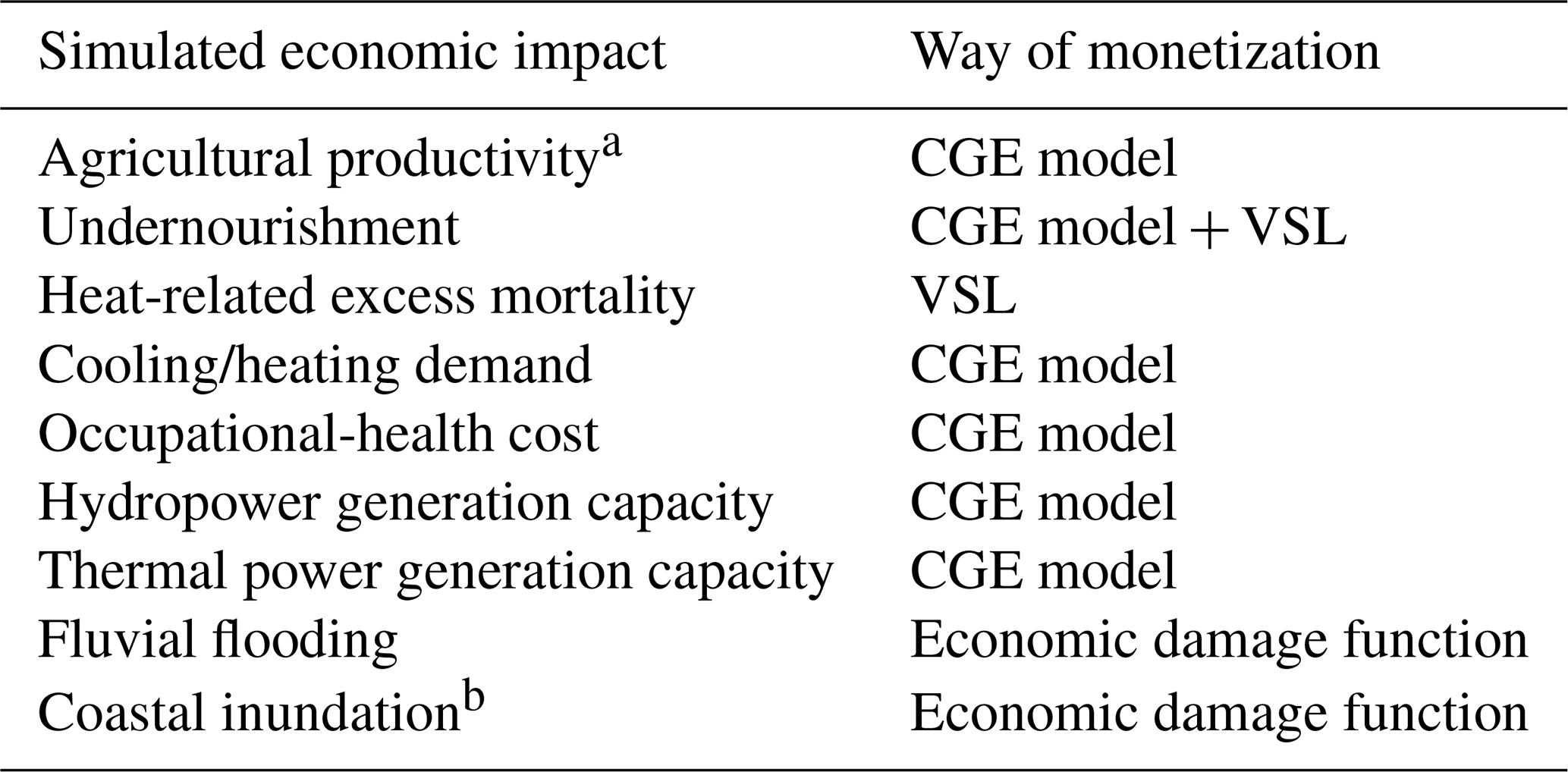
a Definition of the baseline (no-climate-change condition) was changed slightly compared to that of the original study. b Original results imputed by emulation-like technique due to data unavailability.
The simulations were conducted under the shared socioeconomic pathways–representative concentration pathways (SSP–RCP) scenario matrix (van Vuuren et al., 2013). We used five SSPs (SSP1, SSP2, SSP3, SSP4, and SSP5) and four RCPs (RCP2.6, RCP4.5, RCP6.0, and RCP8.5). Moreover, in order to incorporate the uncertainty in climate projections, we used five different global climate models (GCMs), namely, HadGEM2-ES, IPSL-CM5A-LR, MIROC-ESM-CHEM, GFDL-ESM2M, and NorESM1-M (Hempel et al., 2013). Therefore, there are 100 () scenario runs in total. The computational general equilibrium model covers 17 regions (AIM's 17 regions shown in Table S1 in the Supplement), and thus we have economic impacts for these 17 regions (for sectors whose economic impacts can be simulated for each country, the results were aggregated for the 17 regions).
While it is impossible to evaluate how accurate these simulation results are because of inherent uncertainty in the simulations, we regard these simulation results as the ground truth. We used the results of these simulations to construct and evaluate the emulators.
2.2 Overall framework of the emulations
Figure 1 shows the framework of the simulation and the emulation of the economic impacts of climate change. By using the emulators, we want to get results as similar as possible to the results of process-based simulations when the input data or scenario is given. While emulators do not explicitly model the underlying phenomena, they do have parameters, and by tuning these parameters, they can statistically mimic the behaviours (input–output relationship) of simulations.
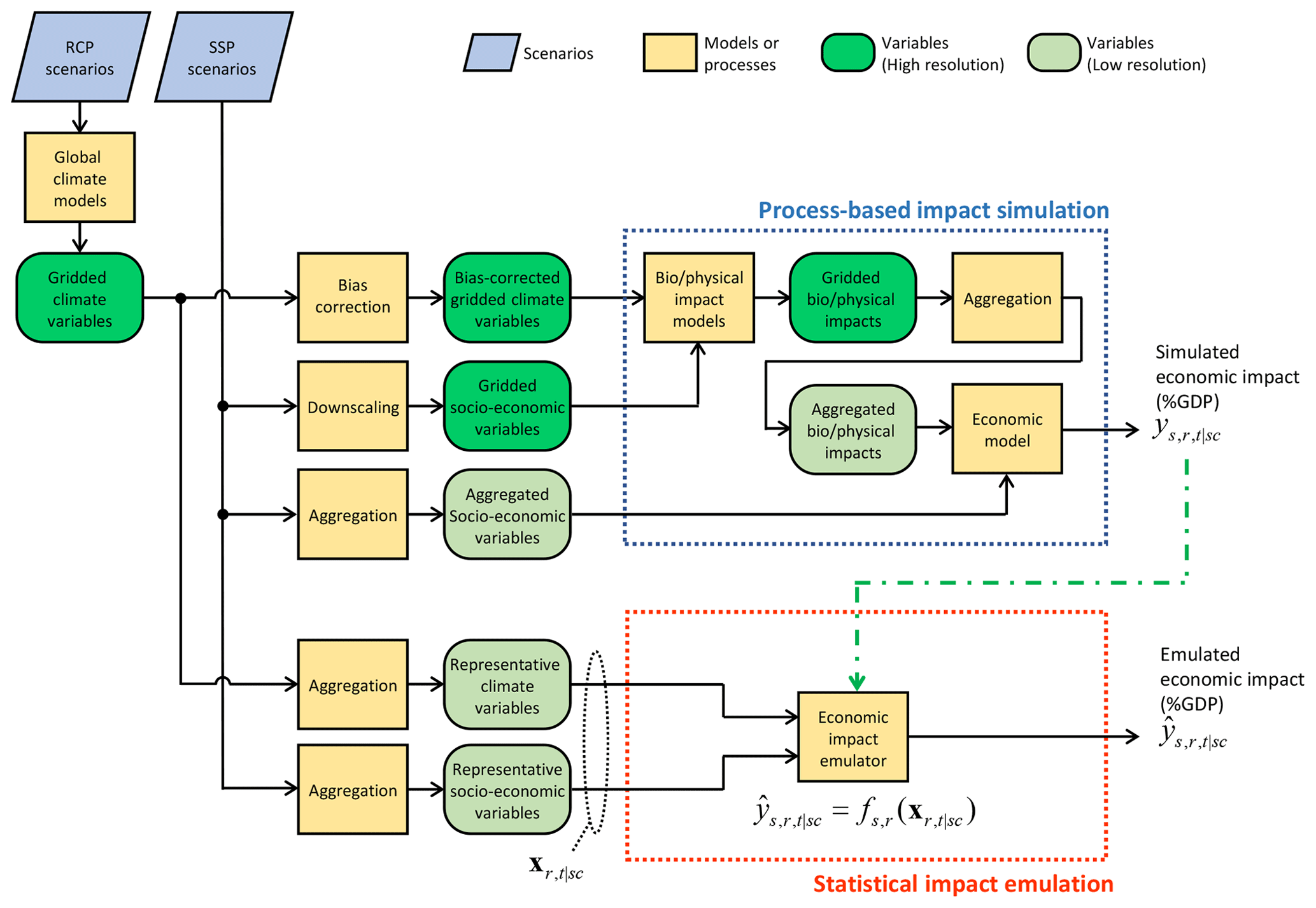
Figure 1Overall framework of simulation and emulation of economic impacts of climate change. Simulated and emulated economic impacts in sector s, region r, and year t under a scenario sc are denoted as and , respectively. The parameters of the emulator are determined based on the simulated economic impact (represented by the green dash–dot–dash arrow).
Here, denotes the simulated economic impact (in percentage of GDP) in sector s, in region r, in year t, and under a given scenario sc, and is the corresponding emulated economic impact. A scenario sc comprises the combination of SSP, RCP, and GCM. The emulated economic impact is calculated by the function receiving the input xr,t|sc as expressed in Eq. (1).
The emulator (function ) is constructed for each sector and region. The input xr,t|sc is the (vector of) variable(s) which is used to emulate the economic impact in region r in year t under a given scenario sc. One important characteristic of the input xr,t|sc is that there is no suffix s. This means that the input variable is not sector-specific and common input data can be used across sectors.
2.3 Tested emulators
2.3.1 Functional forms
We tested a variety of emulators (different functional forms and input variables) ranging from very parsimonious to complex alternatives. For the functional forms, we used ordinary least squares regression (OLS1), ordinary least squares regression with square terms (OLS2), ordinary least squares regression with square and product terms (OLS2i), multi-layer perceptron (MLP), and a recurrent neural network composed of long short-term memory units (LSTM). For the sake of simplicity, we omit the suffixes s, r, and sc in this section, and the ith variable in vector xt is denoted as xt,i.
OLS1 is the simplest form of the emulator, expressed as Eq. (2).
OLS2 includes squared terms and thus can express some curvature in the response.
OLS2i has product terms as well as squared terms, and it can represent some types of interactions among variables.
Simple regressions such as these are widely used, but their capability to express complex phenomena is limited. Currently, more elaborate methods based on statistical machine learning techniques such as ANNs are available. Thus, to represent more complex non-linearities and interactions among variables, we also applied ANN-based techniques to the emulations. MLP is a traditional, but effective and widely used, ANN-based technique that can be applied to the purpose of regression and thus to the emulation. LSTM is also an ANN-based technique designed to handle time-series data and can represent time-dependent characteristics of the data (e.g. cumulative effects in the economic impacts) as well as non-linearities and interactions among variables. Thus, it may better act as the emulator if time-series data are available as the input. While their strict mathematical formulations are lengthy, MLP can be expressed as
where W is the weights (parameters) of the model. LSTM has time-dependent internal state st, and the output and the internal state at time t can be expressed as
See, for example, Goodfellow et al. (2016) for details on MLP and LSTM. Hyperparameters in the ANN-based models were determined based on preliminary examinations. The number of hidden layers and the number of units in each layer were set to 2 and 32, respectively, and the early-stopping technique was used to avoid overfitting of the models.
2.3.2 Input variables
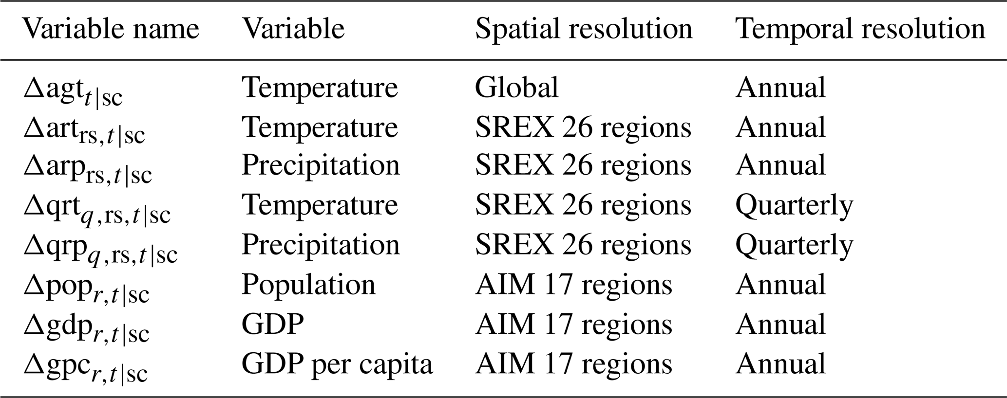
When inputting climate conditions into the emulators, the dimension of the data should be reduced. One typical way to do this is to spatially and temporally aggregate the high-resolution original data. For climate data, the most parsimonious choice involves using the global mean temperature, but this method cannot represent regional and seasonal characteristics of climate conditions. Precipitation also plays an important role for some specific sectors (e.g. hydropower generation capacity, fluvial flooding). We prepared several kinds of input data with different spatial and temporal resolutions by aggregating daily gridded near surface temperature and precipitation data generated by GCMs in CMIP5 (Taylor et al., 2011). First, the spatial resolution of the gridded GCM output data was downscaled to 0.5×0.5∘ by bilinear interpolation. We denote this downscaled gridded temperature as tt|sc(g,d) and precipitation as pt|sc(g,d), where g denotes grid and d denotes day of the year. We calculate annual global mean temperature, annual regional mean temperature and precipitation, and quarterly regional mean temperature and precipitation as follows.
Here, is the number of days in year t, and is the number of days belonging to quarter of a year q. Quarters are grouped following the calendar year, namely, January–February–March, April–May–June, July–August–September, and October–November–December. Coefficient wg is a weight which is proportional to the area of the grid g. Regions are indicated by the subscript rs. Note that rs is based on the classification of SREX's 26 regions defined in IPCC (2012) and different from r (Table S2 in the Supplement). While our interest is estimating the economic impacts in each of AIM's 17 regions represented by r, each such region contains different climate zones because r is classified from the viewpoint of economic modelling rather than climatic and geographic conditions. Thus, to incorporate heterogeneity in climate conditions within an AIM region, we use rs instead of r to define climate variables.
For socioeconomic variables, values are based on the SSP scenarios (Kc and Lutz, 2017; Dellink et al., 2017). Based on the population (popt|sc(c)) and GDP (gdpt|sc(c)) in country c in year t under a given scenario sc, regional population, GDP, and GDP per capita are calculated as follows. GDP is measured in USD (2005) based on the market exchange rate.
When inputting variables to the emulators, it is desirable that their values be within a limited range to ensure the stability of numerical computation. Effects of biases in GCMs should also be alleviated. For this purpose, we used the relative changes of these variables as inputs to the emulators. For temperature, changes were defined by the difference from the base-period (1991–2010) values. For the other variables, changes were defined by a log ratio to the base-period or base-year (2005) values (Table 2).
Table 2Candidate input variables. Socioeconomic variables are defined for AIM's 17 regions, while climatic variables are defined for SREX's 26 regions.
2.4 Comparison
As explained in Sect. 2.3, we have various types of emulators (functional forms) and candidate input variables. We conducted comparisons under selected practically relevant conditions among the possible combinations.
2.4.1 Comparison 1
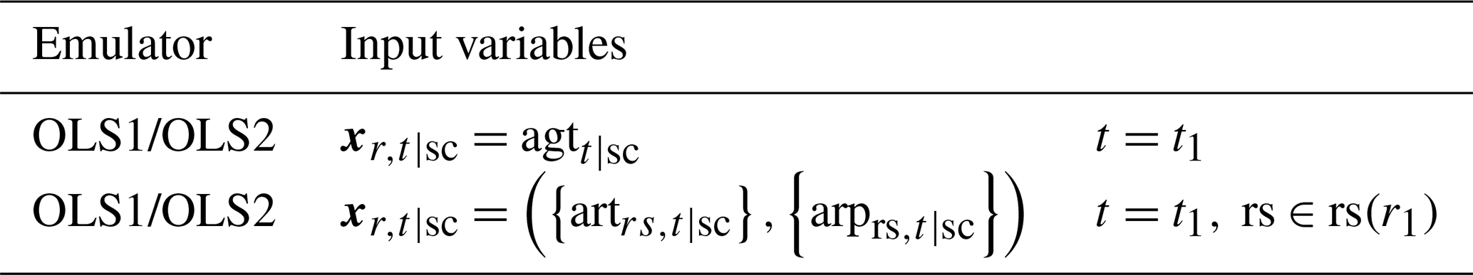
We quantified the performance of the very simple damage functions (OLS1 and OLS2), which only consider the global mean temperature, and compared the performance when regional climate conditions were considered (Table 3). Here, rs(r) represents a set of SREX regions corresponding to an AIM region r (Table S3 in the Supplement).
Table 3Models and input variables in comparison 1. Input variables are used to emulate the economic impact in year t1 in region r1 for each sector.
2.4.2 Comparison 2
We investigated the effects of considering socioeconomic conditions. It is also expected that there are interactions between climate conditions and socioeconomic conditions. To identify whether such interactions can be expressed by a simple method, we included product terms in OLS2i (Table 4).
Table 4Models and input variables in comparison 2. Input variables are variables used to emulate the economic impact in year t1 in region r1 for each sector.
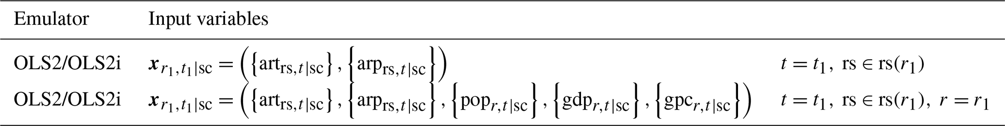
Table 5Models and input variables in comparison 3. Input variables are variables used to emulate the economic impact in year t1 in region r1 for each sector.

Table 6Models and input variables in comparison 4. Input variables are used to emulate the economic impact in year t1 in region r1 for each sector.
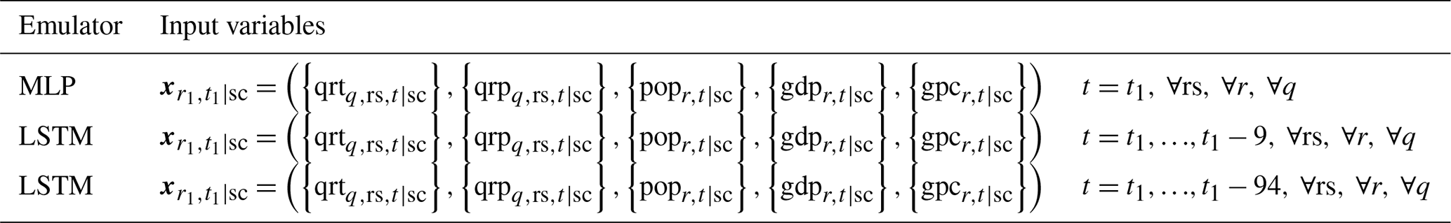
2.4.3 Comparison 3
In comparisons 1 and 2, relatively simple functional forms and temporally coarsely aggregated (annual) climate variables are used. Such an aggregation possibly causes loss of information. For example, crop models consider crop calendars, and thus the temperature changes in growing and non-growing seasons have different effects on their original simulation results. Regarding the economic impacts, climatic and socioeconomic conditions of the non-target regions can also affect the target region through, for example, trade in the international market, which is simulated by the AIM/Hub model. To investigate these possibilities, seasonal climate variables, climate variables of non-target regions, and socioeconomic variables of non-target regions were included as input variables. Moreover, when the number of input variables becomes large, more complex functional forms may be more suitable. Thus, we tested OLS2 and MLP using these variables (Table 5).
2.4.4 Comparison 4
In the previous comparisons, only simultaneous data were used; that is, when emulating the economic impacts in year t, climate and socioeconomic conditions in year t are used. Cumulative or carry-over effects can also exist in the simulated impacts. Therefore, including climate and socioeconomic conditions in past years as the input to the emulator can also contribute to better reproduce the results of the economic simulation. To evaluate the effects of inclusion of information in past years, we tested the performance of artificial neural networks which can consider time-series information (LSTM) with time-series data of different length (10-year data to capture relatively short-period effects and 95-year data which can capture the entire simulation period as shown in Table 6).
2.5 Evaluation
2.5.1 Evaluation procedure metrics
Parameters in the emulators are optimized based on the simulation results. If, however, we simply optimized these parameters based on the existing data (simulation results) and evaluated them by the same data, the performance of the emulators might be overestimated compared to the situation in which new data are input to the emulators. This phenomenon is known as overfitting or overlearning. To avoid the effects of overfitting, we use the cross-validation strategy. We have simulation results for 100 scenarios (), and each scenario has 95 (2006–2100) data points. We divide the 100 scenario results into 4 groups randomly. Three-quarters of the data were used to optimize parameters in the emulators (training), and prediction values were obtained for the remaining one-quarter of the data (test). This procedure was repeated four times by changing the training and test data, and then we got the results of emulation for all scenarios. That is, 4-fold cross-validation was performed.
In some situations, we want to emulate impacts under scenarios which are drastically different from the scenarios which are used to develop (or train) the emulators. In order to evaluate the performance of the emulators under such situations, we also conducted cross-validation by GCM and RCP. Cross-validation by GCM means that the emulators are trained by the simulation results of four GCMs () and tested by the results of the remaining one GCM (). Cross-validation by RCP mean that the emulators are trained by the simulation results of three RCPs () and tested by the results of the remaining one RCP ().
Optimization of the parameters (training) and prediction (test) of OLS-based emulators were conducted using the lm function in R 3.4.3 (R Core Team, 2017). ANN-based emulators were trained and tested using the Keras library (Chollet, 2015) in Python 3.7.3. The Windows operating system (OS) was used in all cases.
2.5.2 Evaluation metrics
The performance of the emulators was evaluated based on the agreement between the results of the simulations and the emulations. By a chosen emulator, we obtain the values of emulated economic impacts . We also have the values of the corresponding original simulated economic impact . We measured the agreement between and by correlation coefficient (r), root mean squared error (RMSE), ratio of RMSE to standard deviation (RSR), and systematic error (bias). These metrics were calculated for each sector and region.
The computational cost of the emulators was assessed by the number of required input data, the number of parameters in a model, model object size (memory size required to load a model), prediction time, and training time. This was measured on a PC (CPU: Intel Core i7–8700K (3.70 GHz, 6 cores/12 threads); RAM: 32 GB; OS: Windows 10 Pro). While the lm function in R was used for OLS-based emulators in the development, they were transplanted to Python for the assessment of computational cost. Thus, both OLS-based emulators and ANN-based emulators were assessed under equal conditions.
We report results for r in the main text since the three metrics (r, RMSE, and RSR) varied almost parallelly, and systematic errors (biases) were nearly negligible for all conditions. Summarized results beyond r (RMSE, RSR, and bias) are available in Tables S4 to S13 in the Supplement, and individual values for all sectors and regions are available as electronic supplementary material. A higher value of r (i.e. r closer to 1) indicates that results of the emulation are similar to those of the simulation when the biases are negligible. The value of r also indicates how well the variation in the simulation results is reproduced by the emulation (square of r is equal to the coefficient of determination or the proportion of explained variance).

Figure 2Performance of emulations in comparison 1. Correlation coefficients between simulation results and emulation results are shown. Bars and edges of boxes represent medians and first/third-quantile values among 17 regional results. The ends of the whiskers show the minimum and maximum values, while outliers are denoted by dots if they exist.
Figure 2 is the results of comparison 1. While there is a large variation in the performance of the emulations for individual sectors, the performance for the aggregated economic impacts is relatively good on average even if they only consider global mean temperature rise. This implies that using simple damage functions can be useful to grasp the rough picture of economic impacts of climate change. On the other hand, when we focus on more minute components, a more elaborate method is required. The effects of including regional climate conditions are distinct in the economic impacts of thermal power generation and fluvial flooding, whose impacts are strongly affected by local precipitation and river flows.

Figure 3Performance of emulations in comparison 2. Correlation coefficients between simulation results and emulation results are shown.
By incorporating socioeconomic variables as inputs to the emulators, there were significant improvements in the performance of the emulations (Fig. 3). The impacts of climate change are determined not only by hazards (climate conditions) but also by exposure and vulnerability (socioeconomic conditions) (IPCC, 2014). Most current-generation simulations of economic impacts, including the simulations used in this study, take socioeconomic aspects into account. Thus, it is not surprising that emulators could better reproduce the results of simulations by taking socioeconomic variables into account. Note that there is very little improvement in the results with respect to river flooding impacts. This is mainly because the same proportion of the population and GDP distribution data were used in the simulation of the impacts of fluvial flooding across SSPs due to data availability (Takakura et al., 2019), and the simulated economic impacts (percentage of GDP) were very similar regardless of the socioeconomic conditions.

Figure 4Performance of emulations in comparison 3. Correlation coefficients between simulation results and emulation results are shown. CA(1) denotes that climate variables for all regions (including non-target region) are used. CS(1) denotes that seasonal climate variables are used. SA(1) denotes that socioeconomic variables for all regions (including non-target region) are used.
Inputting more detailed information improves the performance of the emulations. These improvements were more pronounced when more complex functional forms (MLP) were used. The performance of MLP was comparable to or worse than that of OLS2 when courser input variables were used (leftmost plots in each panel in Fig. 4), whereas MLP performed better when finer input variables were used (rightmost plots) in most cases. The relative importance of variables differs depending on the modelled sectors. For example, for the agricultural productivity and undernourishment sectors, the inclusion of socioeconomic variables in non-target regions contributed to the improvement in performance. The performance for the fluvial flooding sector jumps when seasonal climate variables and climate variables in non-target regions are used with MLPs. This is probably due to the result of “leakage” (discussed later).
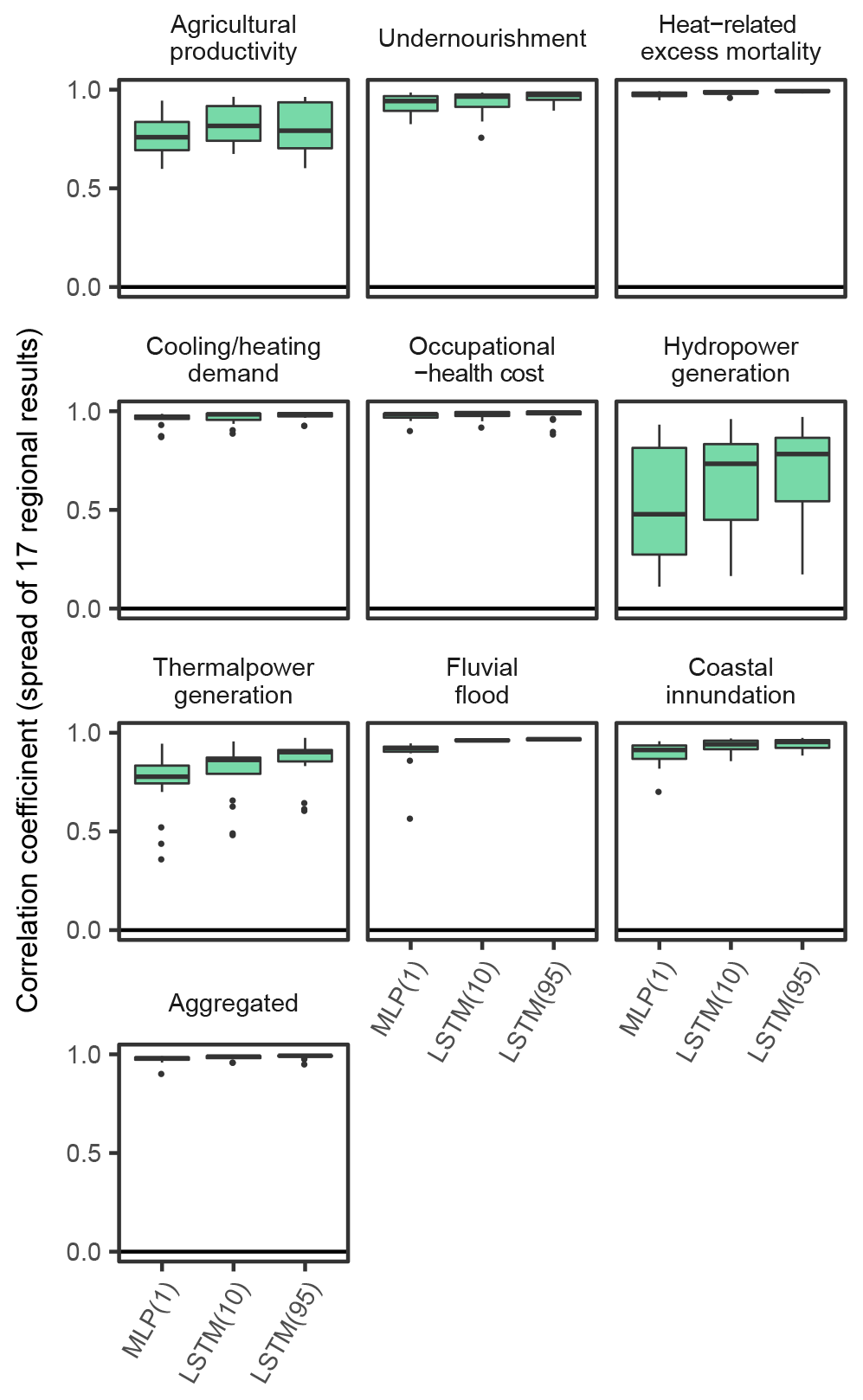
Figure 5Performance of emulations in comparison 4. Correlation coefficients between simulation results and emulation results are shown. MLP(1) denotes that MLPs are used as the emulators and that only climatic and socioeconomic variables for the target year are used. LSTM(10) and LSTM(95) denote that LSTMs are used as the emulators and that the climatic and socioeconomic variables for 10 and 95 years are used, respectively.
Consideration of time-series input variables had positive effects for almost all sectors (Fig. 5), but it had greatest effects in the hydropower generation sector (the median r improves from 0.48 to 0.78). This was mainly because LSTM could reproduce the pre-processing of bio/physical impact simulations before inputting to the economic models. For example, in the simulation of the hydropower generation sector, calculated physical impacts (theoretical hydropower potential) were averaged for every 20 years, and then temporal linear interpolation was applied because this study focused on long-term potential changes due to climate change rather than year-by-year variations (Zhou et al., 2018b). Temporal moving averaging of biological impacts (yields) was also used in the simulations of agricultural productivity and undernourishment. When the original simulations are conducted using these temporally rounded input data, year-by-year input data do not reproduce the original simulation results well. These effects are more obvious when comparing the time-series results of emulation (for example, see Fig. 10), and the results played out just like a low-pass filter had been in place.
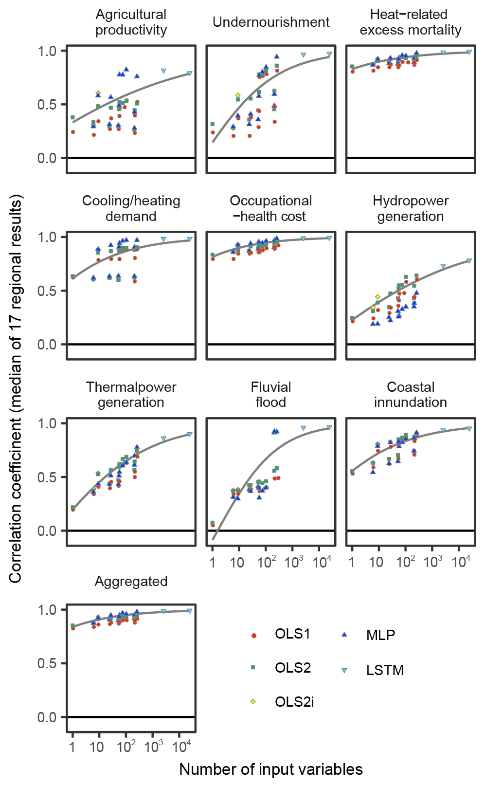
Figure 6Relationship between number of input variables and performance of emulators. Medians of 17 regional results are plotted as points. Fitted curves are produced for the frontiers (Pareto optimal corresponding to each number of input variables) by beta regression. When time-series input data are used, the number of input variables is multiplied by the length of the time series.
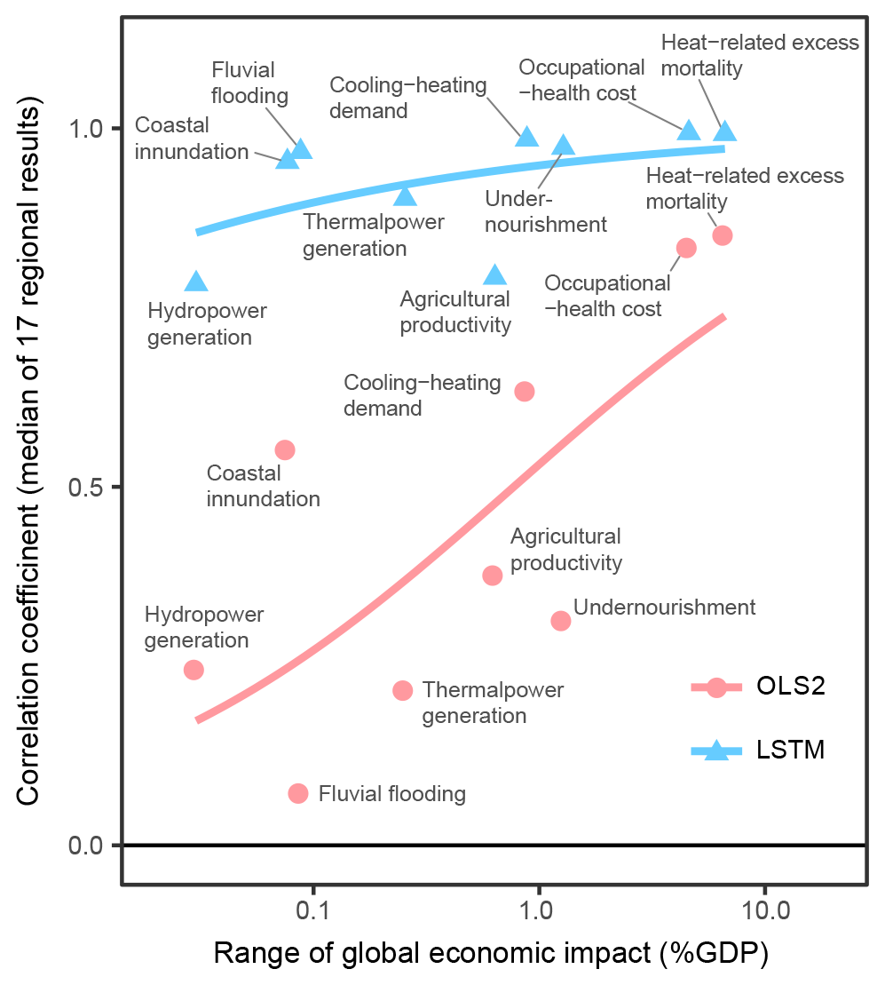
Figure 7Relationship between range of economic impacts (global) and performance of emulators. Each point represents a sector, and the median of 17 regional results is plotted as the y axis value. Fitted curves are produced by beta regression. OLS2 uses only the global mean temperature as the input variable, and LSTM uses all the prepared input variables for 95 years.
In general, the more explanatory variables and the more complex functional forms we use, the better the emulators reproduce the results of the simulations. While this tendency is common for all sectors, there are substantial differences in performance between sectors (Fig. 6). This means some sectors' economic impacts are relatively easy to emulate, but others are more difficult even if the complex techniques are used. There were correlations between impact magnitudes and the performance of the emulators (Fig. 7). That means larger impacts tend to be easier to emulate, and consequently aggregated impacts are also relatively easy to emulate.
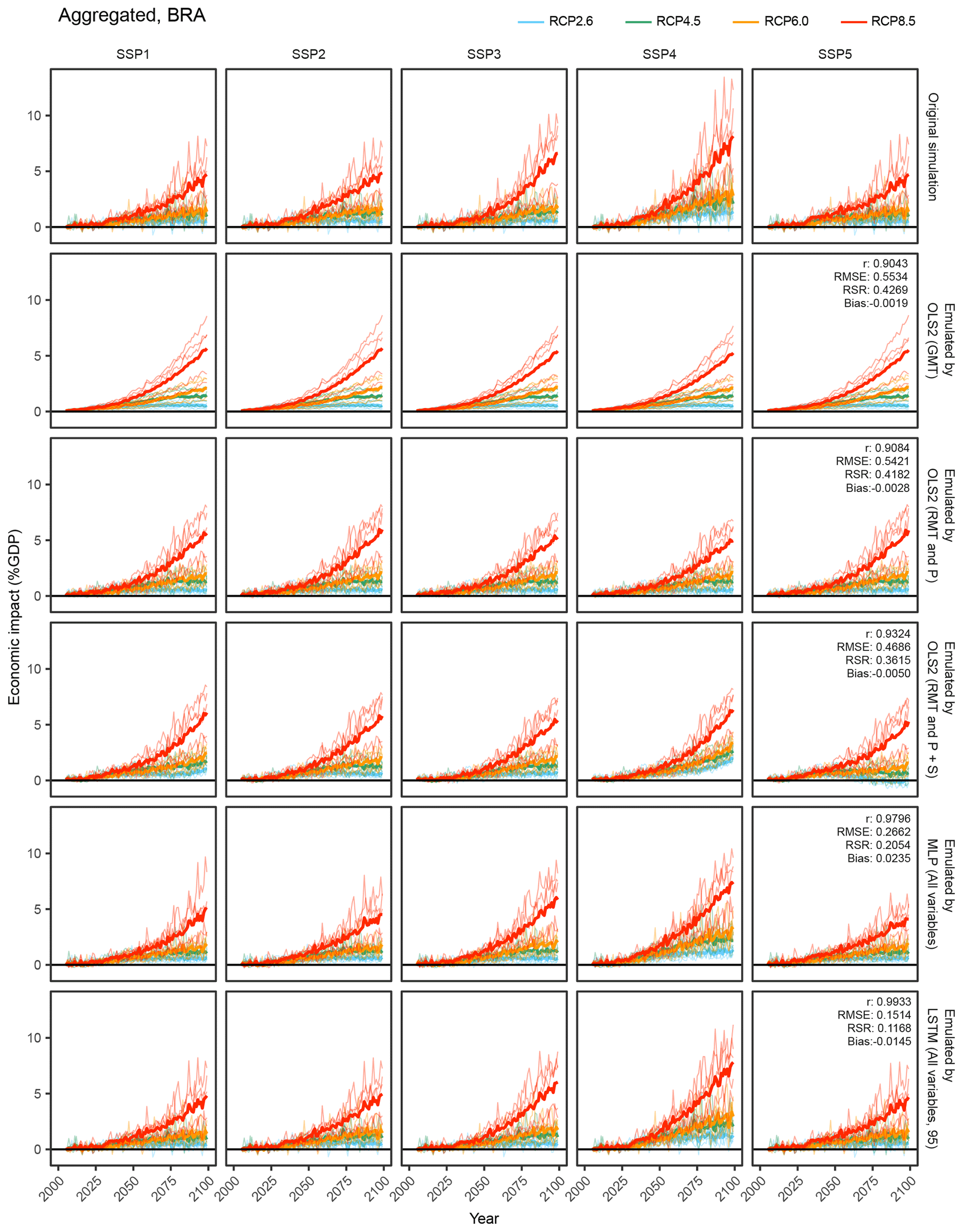
Figure 8Time-series results of the simulation and emulations for aggregated economic impacts in the Brazil region. OLS2 (GMT): OLS2 with global mean temperature. OLS2 (RMT and P): OLS2 with regional mean temperature and precipitation. OLS2 (RMT and P+S): OLS2 with regional mean temperature precipitation and socioeconomic variables. MLP (All variables): MLP with all the input variables. LSTM (All variables, 95): LSTM with all the input variables for 95 years. Thin lines represent individual GCM results, and bold lines represent average of five GCMs.
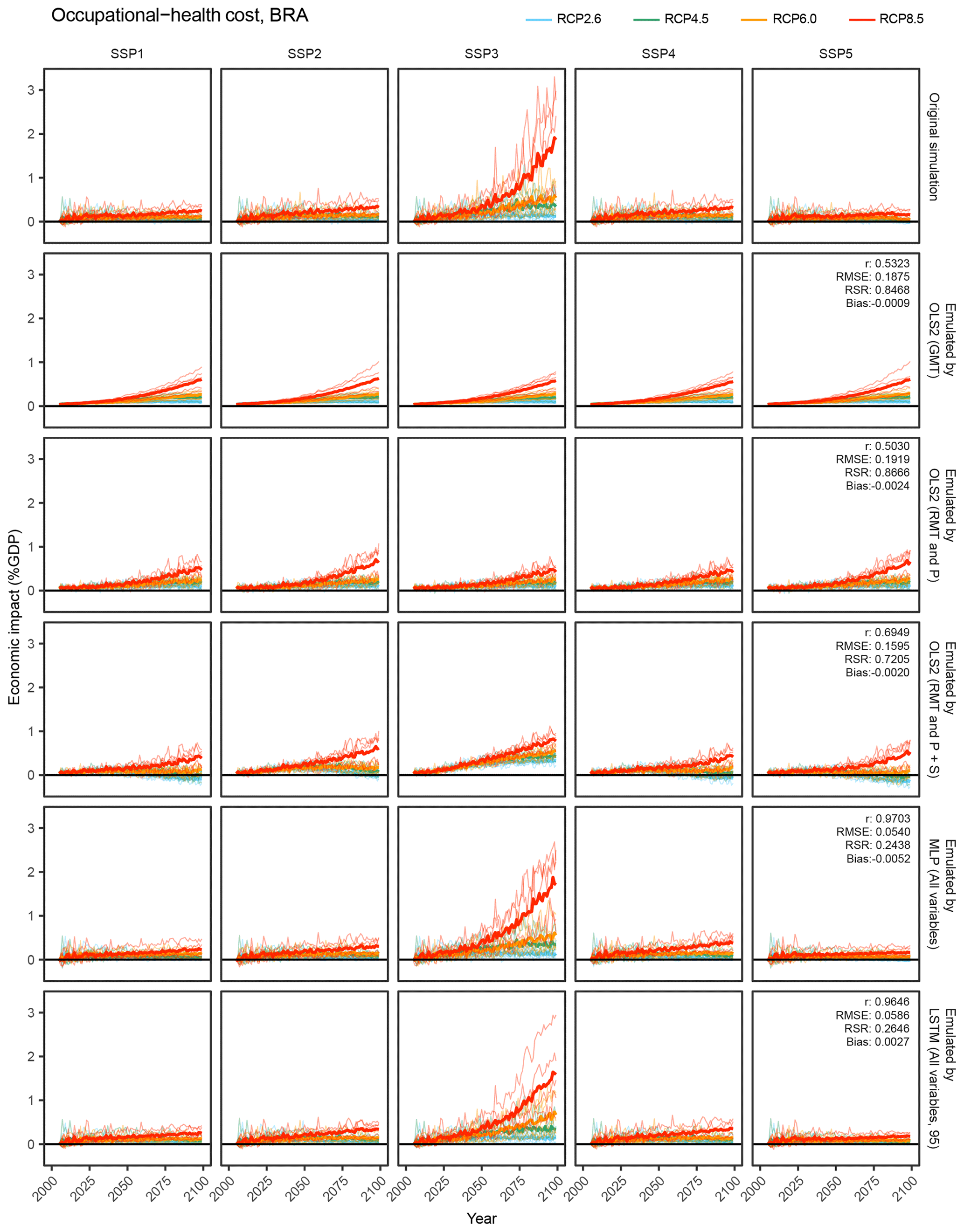
Figure 9Time-series results of the simulation and emulations for the occupational-health cost sector in the Brazil region. OLS2 (GMT): OLS2 with global mean temperature. OLS2 (RMT and P): OLS2 with regional mean temperature and precipitation. OLS2 (RMT and P+S): OLS2 with regional mean temperature precipitation and socioeconomic variables. MLP (All variables): MLP with all the input variables. LSTM (All variables, 95): LSTM with all the input variables for 95 years. Thin lines represent individual GCM results, and bold lines represent average of five GCMs.
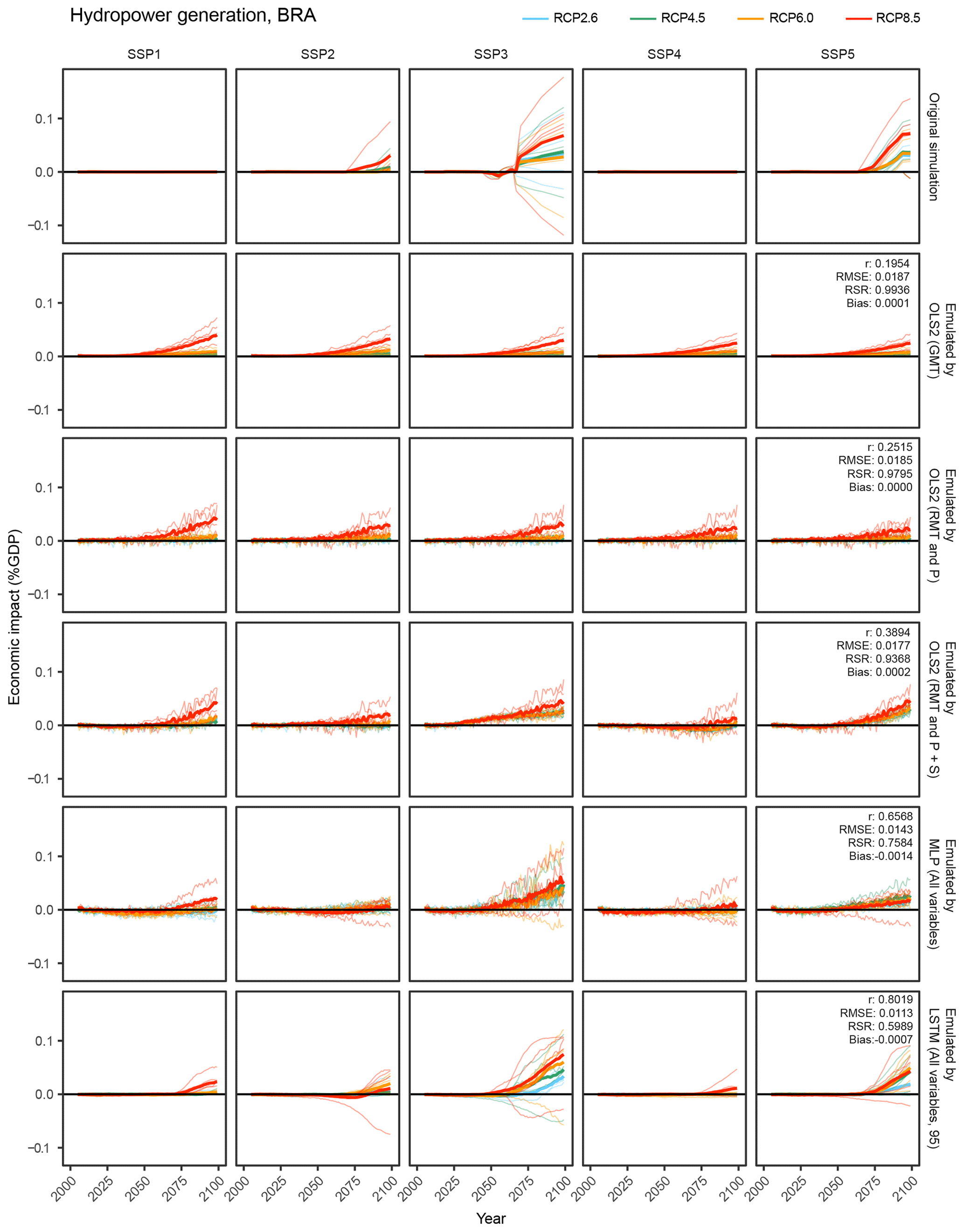
Figure 10Time-series results of the simulation and emulations for the hydropower generation sector in the Brazil region. OLS2 (GMT): OLS2 with global mean temperature. OLS2 (RMT and P): OLS2 with regional mean temperature and precipitation. OLS2 (RMT and P+S): OLS2 with regional mean temperature precipitation and socioeconomic variables. MLP (All variables): MLP with all the input variables. LSTM (All variables, 95): LSTM with all the input variables for 95 years. Thin lines represent individual GCM results, and bold lines represent average of five GCMs.
As illustrative examples, we explore simulated and emulated results for chosen sectors in “Brazil” (Figs. 8, 9, and 10). The top row in each figure shows the time series of simulated economic impacts for each scenario, and the remaining rows show corresponding emulated economic impacts by different emulators. For aggregated economic impacts, general tendencies could be reproduced even by simple emulators, while complex emulators considering socioeconomic conditions could better represent subtle differences among SSPs (Fig. 8). For occupational-health cost sector and hydropower generation sector impacts, obvious differences among SSPs in the simulation results could not be reproduced by simple emulators, but ANN-based complex emulators could reproduce the general tendencies (Figs. 9 and 10). For the hydropower generation sector, even the most complex emulator failed to reproduce some characteristics of the simulation results; that is, the emulator erroneously predicted discernible economic impacts under SSP1 and SSP4.
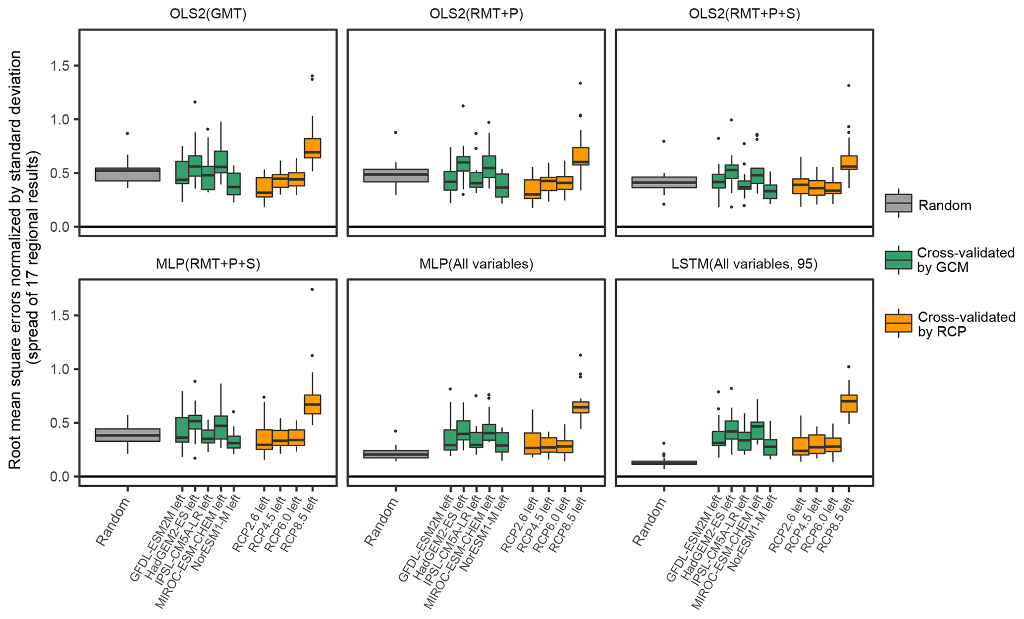
Figure 11Performance of emulations of the aggregated impacts under different cross-validation procedures. Root mean squared errors (normalized by pooled standard deviation) between simulation results and emulation results are shown. Unlike the correlation coefficient, a higher value means a larger error. Random means training and test scenarios are selected randomly. For example, “GFDL-ESM2M left” denotes that the emulators are trained by the results of HadGEM2-ES, IPSL-CM5A-LR, MIROC-ESM-CHEM, and NorESM1-M and then tested by the results of GFDL-ESM2M. Similarly, for example, “RCP2.6 left” denotes that the emulators are trained by the results of RCP4.5, RCP6.0, and RCP8.5 and then tested by the results of RCP2.6. OLS2 (GMT): OLS2 with global mean temperature. OLS2 (RMT+P): OLS2 with regional mean temperature and precipitation. OLS2 (): OLS2 with regional mean temperature precipitation and socioeconomic variables. MLP (): MLP with regional mean temperature precipitation and socioeconomic variables. MLP (All variables): MLP with all the input variables. LSTM (All variables, 95): LSTM with all the input variables for 95 years.
The performance of emulation can vary depending on how the training and test data are chosen. The results shown above are based on cross-validation with randomly selected scenarios for training and testing. Figure 11 shows the comparison of the performance between different cross-validation procedures for the aggregated impacts as an example. Here, the performance is shown by the RMSE normalized by the pooled standard deviation (RSR), not by the correlation coefficient, because the standard deviation of each test data formulation, which affects the value of the correlation coefficient, differs across the selected GCMs or RCPs. Summarized results for each sector and indices beyond RSR (r, RMSE, and bias) are available in Tables S14 to S33 in the Supplement. When the emulators were trained excluding the results of RCP8.5 (the highest emission pathway) and then tested by the results of RCP8.5 (RCP8.5 left condition), the performance was apparently worse compared to the other conditions. Except for RCP8.5 left condition, the performance was reasonably similar across conditions when simpler models and input data were used. When complex models and finer input variables were used, the performance was worse when cross-validated by GCM or cross-validated by RCP compared to the random cross-validation.
Table 7Computational cost of the developed emulators. Medians (minimum, maximum) of 17 regional, 9 sectoral, and aggregated impact results are shown. OLS-based models and ANN-based models were implemented by the statsmodels library and Keras library in Python, respectively. OLS2 (): OLS2 with regional mean temperature precipitation and socioeconomic variables. MLP (): MLP with regional mean temperature precipitation and socioeconomic variables. MLP (All variables): MLP with all the input variables. LSTM (All variables, 95): LSTM with all the input variables for 95 years.
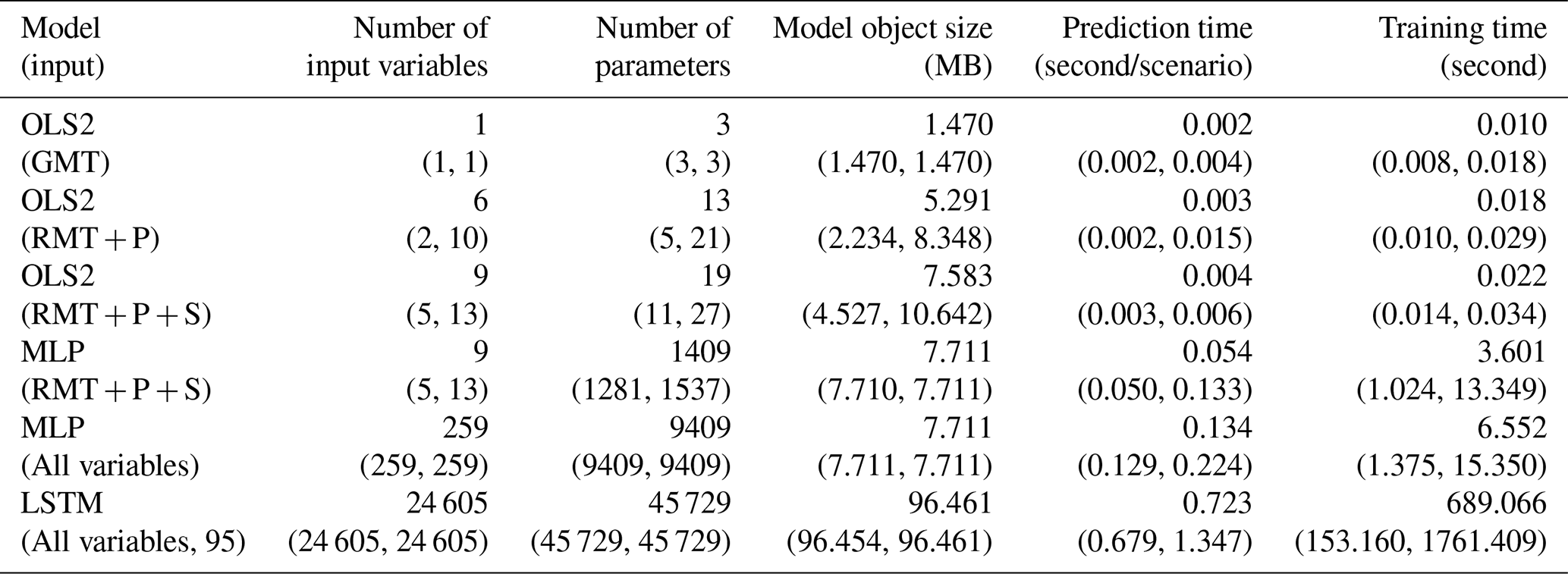
The computational cost of the developed emulators was sufficiently small in the prediction phase, while training requires some time for ANN-based emulators. Table 7 shows the computational cost for selected conditions. Even if the most complex emulators are used, they require only 723 (679 to 1347) ms for the calculation of the economic impact for a century. From the viewpoint of computation time required for the prediction, both the OLS-based and ANN-based models can meet the requirement of the emulators. However, it should be noted that the time required to prepare the input variables is not included in this assessment, and it depends on the situations.
In this study, we developed various kinds of emulators and systematically evaluated their performance. We explored differences in emulator performance among sectors and the relationship between model complexity and performance. The aggregated economic impact was relatively easily emulated even by simple emulators with limited input variables. The dominant contributors of aggregated impact were the heat-related excess mortality and occupational-health cost sectors (Takakura et al., 2019) as also shown in Sect. S2 in the Supplement, and the economic impacts of these two sectors were also relatively easily emulated. There were clear relationships between temperature rise and the simulated impacts in these two sectors (Honda et al., 2014; Takakura et al., 2017), and almost all regions were impacted in the same direction. Moreover, where impacts were large, emulator performance tended to be better as shown in Fig. 7. Temperature-dependent impacts tend to be large and easy to emulate, while precipitation-dependent impacts tend to be small and difficult to emulate. Although it is not clear whether this correlation reflects a causal relationship or is just a coincidence, these characteristics contributed to the higher performance of emulations of aggregated impacts particularly when simple functional forms were used. If we only focus on the aggregated economic impacts of climate change, a simple damage function which only leverages global mean temperature is worth using provided that we regard the original simulation results as valid. On the other hand, some sectors' and regions' impacts were difficult to emulate by simple emulators, and consideration of more input variables and more complex functional forms could improve the performance. Therefore, if we focus on sectoral or regional issues (e.g. inequality among regions or sectors), conventional simple damage functions may not be adequate tools and ANN-based or other complex techniques may be necessary.
For the agricultural productivity and undernourishment sectors, the performance of the emulations was low unless socioeconomic conditions of non-target regions were incorporated. Since comparative advantages (or disadvantages) in the international food market and global food demands play important roles in simulations of the impacts in these sectors, it is reasonable that non-target regional information contributed to improve the performance of the emulations. Such beyond-the-border effects have not been considered in previous studies using damage functions or emulators, but our results shed light on the importance of this factor. It is also noteworthy that these improvements were more distinct when MLPs, which can represent complex interactions among variables, were used as the emulators.
In terms of the results for the fluvial flooding sector, inclusion of non-target regions' quarterly climate variables with MLP caused a drastic jump in the performance of the emulators. This is puzzling because in the simulation of the impacts of fluvial flooding, effects of international trading are not considered explicitly (Kinoshita et al., 2018). We suspect this is caused by the leakage because of the characteristics of the simulation data used in this study. In the field of statistical machine learning, the word leakage means that models have access to some information on the characteristics of the test dataset even if the test and training datasets are separated (Kaufman et al., 2011). In this study, we separated the dataset into training and test datasets depending on the scenarios. When a certain scenario (for example, SSP1-RCP2.6-HadGEM2-ES) is used in the test dataset, it is not included in the training dataset. By doing this, we can evaluate how the trained emulators will work when a new unknown scenario is given. However, in the case of fluvial flooding, the simulated impacts expressed by percentage of GDP are very similar among SSPs (Takakura et al., 2019). For example, the simulated impacts (percentage of GDP) in SSP1-RCP2.6-HadGEM2-ES are almost identical to those in SSP2-RCP2.6-HadGEM2-ES, SSP3-RCP2.6-HadGEM2-ES, SSP4-RCP2.6-HadGEM2-ES, and SSP5-RCP2.6-HadGEM2-ES, and some of these datasets are included in the training dataset. In such a situation, overfitting can result in apparently high performance in the cross-validation even if its actual ability for a new input dataset is low. Therefore, apparently high performance in the fluvial flood sector should be interpreted with caution.
In the sectors of hydropower generation and thermal power generation, even using the complex emulators with finer input variables, the attained performance remained relatively low. This implies that information required to reproduce the simulation results is missing from the input data. In the AIM/Hub model, there are SSP-dependent assumptions other than population and GDP, particularly related to energy policies (Fujimori et al., 2017). These policies depend on the narratives of the SSP storylines, not just quantitative socioeconomic information such as population or GDP. In addition, in the AIM/Hub model, adoption of power generation technology is decided by a discrete-choice model (Fujimori et al., 2014). Thus, the degree of reliance on a certain kind of power generation can also be discrete or non-continuous depending on the SSP-dependent assumptions in the AIM/Hub model. For example, a certain region does not rely on the hydropower generation at all in some situations, but once the hydropower generation technology becomes economically competitive compared to other power generation technologies, hydropower generation plants will be installed in the model. In the former situation, changes in the hydropower generation capacity do not affect the economy at all, but they do in the latter situation. This difference cannot be predicted by the emulators, since they cannot be represented only by climate conditions, GDP, and population.
To improve the performance of the economic impact emulations, should we construct more complex emulators and consider more information? For example, in power generation sectors, model-specific assumptions regarding the energy system could be used as additional input variables and this might improve the emulation performance. If a sufficient number of simulation results are available, this strategy may work. An alternative approach is refraining from reproducing the complex behaviour of the energy system in the simulation model by an emulator and partly using the original simulation model. For example, in simulations of the impacts of hydropower generation and thermal power generation, bio/physical impacts (theoretical hydropower potential and river flow) are simulated by a global hydrological model, whose computational cost is high (around 15 to 20 h for one scenario), while the economic impacts are simulated by an economic model, whose computational cost is relatively low (around 1.5 h for one scenario) compared to that of the hydrological model. Therefore, if we can only emulate bio/physical impacts, the computational cost of economic impact estimation can be reduced even if we use the original simulation model for the economic part. Such model separations will become important particularly if we focus, for example, on interactions among different sectors (Harrison et al., 2016). Another possibility is constructing SSP-specific emulators. In this study, since we aimed to explore new socioeconomic pathways (e.g. intermediate pathway between SSP1 and SSP2), one common emulator was constructed for different socioeconomic pathways. On the other hand, if we fix the socioeconomic pathways to consider, it is possible to incorporate SSP-specific assumptions into the emulators by separating the models by SSPs. This option could be pursued depending on the purpose of the studies.
Even without introducing overly complex models or considering excessively specific information, there are several techniques which may improve the performance of emulation. For example, variable selection is a widely used technique pursuant of developing parsimonious models and avoiding overfitting. We tested the simple step-wise variable selection based on Akaike's information criterion, which can easily be applied to an OLS-based technique, and the results are shown in Sect. S3 in the Supplement. Optimization of the hyperparameters – e.g. the number of units, the number of hidden layers, and the batch size for training in ANN – can also be effective. In addition to optimizing or modifying the models used in this study, other kind of models – such as support vector regression, random forest regression, and k-nearest neighbours regression – may also be effective. If we adopt techniques like Gaussian process regression, uncertainty of the predicted value can also be assessed. While we did not investigate these techniques in this study, this represents an important direction for future research.
While there is substantial room for improvement, the emulators developed in this study can be used as tools to explore various other future scenarios with limited computational and implementation cost. Technically, applying ANN-based techniques to economic impact emulation is one of the novelties of this study, and we have demonstrated that these techniques can improve the performance of the emulations. However, we do not claim researchers should always use ANN-based (or similar statistically complex) techniques in economic impact emulations. There is a non-negligible trade-off between model complexity and performance. While computational cost of emulation is small in the calculation (prediction) phase as shown in Table 7, even by the most complex emulator used in this study, the availability of input variables is context-specific. For example, the cost of preparing or generating sub-yearly regional climate variables should also be considered. We disclose the source code for the OLS-based and ANN-based emulators developed herein. Sector-specific skills and knowledge are not necessarily needed to use this code, and thus the implementation cost is much smaller than that of the original simulation models, particularly if the pre-trained models are used. Nevertheless, transplanting the ANN-based emulators to other modelling languages, if necessary, is not always a trivial task, because of the required software libraries. On the other hand, it is much easier to transplant OLS-based emulators in any modelling language because they only require arithmetic multiplication and addition.
While sector-specific skills and knowledge are not always necessary to use the developed emulators, users should be aware of the statistical context of the emulators and evaluation results. Firstly, cross-validation is a powerful tool for evaluating the emulators' performance without the influence of overfitting, and we can rely on the results of cross-validation to choose adequate models in most cases. However, leakage can pass the cross-validation test unlike simple overfitting. While there is no perfect solution to detect the existence of leakage, it can be effective to think about the actual situation in which the developed emulators will be used. For example, if the emulators will be used to estimate economic impacts under different RCPs or substantially different emission pathways, which are not included in the training data, cross-validation by RCPs can be effective to estimate the actual performance of the emulators in that situation. Suspected leakage shown in Fig. 4 can be detected by this strategy (Sect. S4 in the Supplement). Secondly, regression models are not good at extrapolation, as shown in RCP8.5 left condition in Fig. 11. Fortunately, RCP8.5 left condition is a hypothetical situation only for the purpose of the evaluation. In the actual situations in which the emulators will be used, the simulation results under RCP8.5 are included in the training data, and emission pathways higher than RCP8.5 are nearly impossible considering the current world situation (Hausfather and Peters, 2020). Therefore, as for the emission pathway, the problem of extrapolation will not be a serious issue in practical terms, but we should be aware of whether an emulated scenario is inside or outside the range of the original simulations. Thirdly, overfitting should be avoided as a general rule, but some sort of overfitting can be allowed depending on the purpose of the studies. For example, constructing SSP-specific emulators is possible as discussed above. These emulators overfit to the corresponding SSPs (socioeconomic pathways) and thus will not work well under different socioeconomic pathways. On the other hand, as long as the purpose of the emulation is to explore future scenarios other than socioeconomic pathways, overfitting to the SSPs will not be a problem. Such judgements may be difficult. In general, however, unwanted and unexpected characteristics of statistical models tend to emerge when more complex models are used. Therefore, it is conservative, but can be safer, to choose a simpler model if it meets the requirement of the studies when the users are not confident about the model characteristics.
Both simple and complex emulators have advantages and disadvantages. We cannot conclude which emulator is the “best” one, because it depends on the purpose and situation, but we can give a general guideline to choose a suitable emulator based on the results of this study. This is the fact that simple emulators are effective for approximating global general tendencies, but complex emulators are necessary if the focus is regional or sectoral heterogeneity. Through a systematic comparison of different emulators, ranging from very parsimonious through to complex alternatives, the findings of this study can help researchers choose and implement the most suitable emulators for their purposes and situations.
We used the results of simulations as the ground truth, and the emulators were optimized to reproduce the results of the simulations. While we used state-of-the-art simulation results (Takakura et al., 2019), the simulations themselves contain uncertainties and inaccuracies. Thus, even if the emulators could reproduce the results of the simulations, this would not necessarily mean the economic impacts estimated by the emulators are accurate.
In this study, we assumed that climate data from GCMs were given and representative climate variables could be calculated by aggregating (or upscaling) them. On the other hand, particularly when the emulator is used as a component of a typical integrated assessment model, climate data are calculated by a simple climate model, and only the global mean temperature is available. In such a situation, downscaling is necessary if the emulator requires regional or seasonal climate variables. This is possible using, for example, a pattern scaling technique (Herger et al., 2015; Osborn et al., 2016). In this case, the overall performance of the emulation should be evaluated including this pre-processing.
We should also consider the division of roles between models. In this study, the emulators played the roles of both bio/physical impact models and economic models. As discussed above, it can be difficult to incorporate the assumptions used in the economic models into the emulators. To avoid such difficulties, it may be better for emulators to focus on bio/physical impacts, with the economic impacts being calculated by an appropriate economic model. In general, the computational costs of economic models are lower compared to those of bio/physical impact models, and thus it is prudent to consider this option. It may also be desirable from the viewpoint of representing interactions among sectors, but more investigations, model developments, and validations are needed to model complex interactions. The optimal configuration of the model cascade should be decided considering prediction accuracy, computational cost, and the purpose of studies.
Code and data to reproduce the results in this paper are available at https://doi.org/10.5281/zenodo.4692496 (Takakura, 2021). There are two directories in the repository. The directory named RTU contains ready-to-use code and sample data for users of the developed emulators. The directory named REPRODUCTION contains code and data that are required to reproduce the results reported in this paper.
The supplement related to this article is available online at: https://doi.org/10.5194/gmd-14-3121-2021-supplement.
JT conducted the formal analysis and prepared the original draft. JT, SF, KT, NH, TH, YuHi, YaHo, TI, CP, and MT provided the resources. YaHi supervised the study. All authors reviewed and/or edited the manuscript.
Until February 2016, JT was employed by Toshiba Corporation, whose business is related to hydropower and thermal power generation. The other authors declare no competing interests.
This research was supported by the Environment Research and Technology Development Fund (JPMEERF15S11400 and JPMEERF20202002) of the Environmental Restoration and Conservation Agency of Japan.
This paper was edited by Rohitash Chandra and reviewed by two anonymous referees.
Burke, M., Hsiang, S. M., and Miguel, E.: Global non-linear effect of temperature on economic production, Nature, 527, 235, https://doi.org/10.1038/nature15725, 2015.
Castelletti, A., Galelli, S., Ratto, M., Soncini-Sessa, R., and Young, P. C.: A general framework for Dynamic Emulation Modelling in environmental problems, Environ. Modell. Softw., 34, 5–18, https://doi.org/10.1016/j.envsoft.2012.01.002, 2012.
Chollet, F.: Keras, https://github.com/fchollet/keras (last access: 21 July 2019), 2015.
Ciscar, J.-C., Iglesias, A., Feyen, L., Szabó, L., Van Regemorter, D., Amelung, B., Nicholls, R., Watkiss, P., Christensen, O. B., Dankers, R., Garrote, L., Goodess, C. M., Hunt, A., Moreno, A., Richards, J., and Soria, A.: Physical and economic consequences of climate change in Europe, P. Natl. Acad. Sci., 108, 2678, https://doi.org/10.1073/pnas.1011612108, 2011.
Cybenko, G.: Approximation by superpositions of a sigmoidal function, Mathematics of Control, Signals and Systems, 2, 303–314, https://doi.org/10.1007/BF02551274, 1989.
Dellink, R., Chateau, J., Lanzi, E., and Magné, B.: Long-term economic growth projections in the Shared Socioeconomic Pathways, Global Environ. Chang., 42, 200–214, https://doi.org/10.1016/j.gloenvcha.2015.06.004, 2017.
Diaz, D. and Moore, F.: Quantifying the economic risks of climate change, Nat. Clim. Change, 7, 774–782, https://doi.org/10.1038/nclimate3411, 2017.
Fujimori, S., Masui, T., and Matsuoka, Y.: AIM/CGE [basic] manual, Discussion Paper Series, Center for Social and Environmental Systems Research, NIES, 2012.
Fujimori, S., Masui, T., and Matsuoka, Y.: Development of a global computable general equilibrium model coupled with detailed energy end-use technology, Appl. Energ., 128, 296–306, https://doi.org/10.1016/j.apenergy.2014.04.074, 2014.
Fujimori, S., Hasegawa, T., Masui, T., Takahashi, K., Herran, D. S., Dai, H., Hijioka, Y., and Kainuma, M.: SSP3: AIM implementation of Shared Socioeconomic Pathways, Global Environ. Chang., 42, 268–283, https://doi.org/10.1016/j.gloenvcha.2016.06.009, 2017.
Fujimori, S., Iizumi, T., Hasegawa, T., Takakura, J., Takahashi, K., and Hijioka, Y.: Macroeconomic Impacts of Climate Change Driven by Changes in Crop Yields, Sustainability, 10, 3673, https://doi.org/10.3390/su10103673, 2018.
Goodfellow, I., Bengio, Y., and Courville, A.: Deep learning, MIT press, Cambridge, MA, USA, 2016.
Harrison, P. A., Holman, I. P., Cojocaru, G., Kok, K., Kontogianni, A., Metzger, M. J., and Gramberger, M.: Combining qualitative and quantitative understanding for exploring cross-sectoral climate change impacts, adaptation and vulnerability in Europe, Reg. Environ. Change, 13, 761–780, https://doi.org/10.1007/s10113-012-0361-y, 2013.
Harrison, P. A., Dunford, R. W., Holman, I. P., and Rounsevell, M. D. A.: Climate change impact modelling needs to include cross-sectoral interactions, Nat. Clim. Change, 6, 885, https://doi.org/10.1038/nclimate3039, 2016.
Hasegawa, T., Fujimori, S., Takahashi, K., Yokohata, T., and Masui, T.: Economic implications of climate change impacts on human health through undernourishment, Climatic Change, 136, 189–202, https://doi.org/10.1007/s10584-016-1606-4, 2016a.
Hasegawa, T., Park, C., Fujimori, S., Takahashi, K., Hijioka, Y., and Masui, T.: Quantifying the economic impact of changes in energy demand for space heating and cooling systems under varying climatic scenarios, Palgrave Communications, 2, 16013, https://doi.org/10.1057/palcomms.2016.13, 2016b.
Hausfather, Z. and Peters, G. P.: Emissions – the `business as usual' story is misleading, Nature, 577, 618–620, 2020.
Hempel, S., Frieler, K., Warszawski, L., Schewe, J., and Piontek, F.: A trend-preserving bias correction – the ISI-MIP approach, Earth Syst. Dynam., 4, 219–236, https://doi.org/10.5194/esd-4-219-2013, 2013.
Herger, N., Sanderson, B. M., and Knutti, R.: Improved pattern scaling approaches for the use in climate impact studies, Geophys. Res. Lett., 42, 3486–3494, https://doi.org/10.1002/2015GL063569, 2015.
Honda, Y., Kondo, M., McGregor, G., Kim, H., Guo, Y. L., Hijioka, Y., Yoshikawa, M., Oka, K., Takano, S., Hales, S., and Kovats, R. S.: Heat-related mortality risk model for climate change impact projection, Environ. Health Prev., 19, 56–63, https://doi.org/10.1007/s12199-013-0354-6, 2014.
Howard, P. H. and Sterner, T.: Few and Not So Far Between: A Meta-analysis of Climate Damage Estimates, Environ. Resour. Econ., 68, 197–225, https://doi.org/10.1007/s10640-017-0166-z, 2017.
Iizumi, T., Furuya, J., Shen, Z., Kim, W., Okada, M., Fujimori, S., Hasegawa, T., and Nishimori, M.: Responses of crop yield growth to global temperature and socioeconomic changes, Sci. Rep., 7, 7800, https://doi.org/10.1038/s41598-017-08214-4, 2017.
IPCC: Managing the Risks of Extreme Events and Disasters to Advance Climate Change Adaptation. A Special Report of Working Groups I and II of the Intergovernmental Panel on Climate Change, Cambridge University Press, Cambridge, UK, and New York, NY, USA, 2012.
IPCC: Climate Change 2014: Impacts, Adaptation, and Vulnerability. Contribution of Working Group II to the Fifth Assessment Report of the Intergovernmental Panel on Climate Change, Cambridge University Press, Cambridge, UK and New York, NY, USA, 2014.
Kaufman, S., Rosset, S., and Perlich, C.: Leakage in data mining: formulation, detection, and avoidance, Proceedings of the 17th ACM SIGKDD international conference on Knowledge discovery and data mining, San Diego, California, USA, 21–24 August 2011, 556–563, https://doi.org/10.1145/2020408.2020496, 2011.
Kc, S. and Lutz, W.: The human core of the shared socioeconomic pathways: Population scenarios by age, sex and level of education for all countries to 2100, Global Environ. Chang., 42, 181–192, https://doi.org/10.1016/j.gloenvcha.2014.06.004, 2017.
Riahi, K., Bertram, C., Huppmann, D., Rogelj, J., Bosetti, V., Cabardos, A.-M., Deppermann, A., Drouet, L., Frank, S., Fricko, O., Fujimori, S., Harmsen, M., Hasegawa, T., Krey, V., Luderer, G., Paroussos, L., Schaeffer, R., Weitzel, M., van der Zwaan, B., Vrontisi, Z., Dalla Longa, F., Després, J., Fosse, F., Fragkiadakis, K., Gusti, M., Humpenöder, F., Keramidas, K., Kishimoto, P., Kriegler, E., Meinshausen, M., Nogueira, L. P., Oshiro, K., Popp, A., Rochedo, P., Unlu, G., van Ruijven, B., Takakura, J., Tavoni, M., van Vuuren, D., and Zakeri, B.: Long-term economic benefits of stabilizing warming without overshoot – the ENGAGE model intercomparison, Nature Portfolio [preprint], https://doi.org/10.21203/rs.3.rs-127847/v1, 2021.
Kinoshita, Y., Tanoue, M., Watanabe, S., and Hirabayashi, Y.: Quantifying the effect of autonomous adaptation to global river flood projections: application to future flood risk assessments, Environ. Res. Lett., 13, 014006, 2018.
Matsumoto, K.: Climate change impacts on socioeconomic activities through labor productivity changes considering interactions between socioeconomic and climate systems, J. Clean. Prod., 216, 528–541, https://doi.org/10.1016/j.jclepro.2018.12.127, 2019.
Mitchell, D., AchutaRao, K., Allen, M., Bethke, I., Beyerle, U., Ciavarella, A., Forster, P. M., Fuglestvedt, J., Gillett, N., Haustein, K., Ingram, W., Iversen, T., Kharin, V., Klingaman, N., Massey, N., Fischer, E., Schleussner, C.-F., Scinocca, J., Seland, Ø., Shiogama, H., Shuckburgh, E., Sparrow, S., Stone, D., Uhe, P., Wallom, D., Wehner, M., and Zaaboul, R.: Half a degree additional warming, prognosis and projected impacts (HAPPI): background and experimental design, Geosci. Model Dev., 10, 571–583, https://doi.org/10.5194/gmd-10-571-2017, 2017.
Mizuta, R., Murata, A., Ishii, M., Shiogama, H., Hibino, K., Mori, N., Arakawa, O., Imada, Y., Yoshida, K., Aoyagi, T., Kawase, H., Mori, M., Okada, Y., Shimura, T., Nagatomo, T., Ikeda, M., Endo, H., Nosaka, M., Arai, M., Takahashi, C., Tanaka, K., Takemi, T., Tachikawa, Y., Temur, K., Kamae, Y., Watanabe, M., Sasaki, H., Kitoh, A., Takayabu, I., Nakakita, E., and Kimoto, M.: Over 5,000 Years of Ensemble Future Climate Simulations by 60 km Global and 20 km Regional Atmospheric Models, B. Am. Meteorol. Soc., 98, 1383–1398, https://doi.org/10.1175/BAMS-D-16-0099.1, 2017.
Nordhaus, W. D.: Revisiting the social cost of carbon, P. Natl. Acad. Sci., 114, 1518–1523, https://doi.org/10.1073/pnas.1609244114, 2017.
OECD: Mortality Risk Valuation in Environment, Health and Transport Policies, OECD Publishing, https://doi.org/10.1787/9789264130807-en, 2012.
Osborn, T. J., Wallace, C. J., Harris, I. C., and Melvin, T. M.: Pattern scaling using ClimGen: monthly-resolution future climate scenarios including changes in the variability of precipitation, Climatic Change, 134, 353–369, https://doi.org/10.1007/s10584-015-1509-9, 2016.
Oyebamiji, O. K., Edwards, N. R., Holden, P. B., Garthwaite, P. H., Schaphoff, S., and Gerten, D.: Emulating global climate change impacts on crop yields, Stat. Model., 15, 499–525, https://doi.org/10.1177/1471082X14568248, 2015.
Park, C., Fujimori, S., Hasegawa, T., Takakura, J., Takahashi, K., and Hijioka, Y.: Avoided economic impacts of energy demand changes by 1.5 and 2 ∘C climate stabilization, Environ. Res. Lett., 13, 045010, https://doi.org/10.1088/1748-9326/aab724, 2018.
R Core Team: R: A Language and Environment for Statistical Computing, R Foundation for Statistical Computing, 2017.
Schnorbus, M. A. and Cannon, A. J.: Statistical emulation of streamflow projections from a distributed hydrological model: Application to CMIP3 and CMIP5 climate projections for British Columbia, Canada, Water Resour. Res., 50, 8907–8926, https://doi.org/10.1002/2014WR015279, 2014.
Stern, N.: The Economics of Climate Change: The Stern Review, Cambridge University Press, Cambridge, UK, 2006.
Takakura, J.: Code and data for the paper “Reproducing complex simulations of economic impacts of climate change with lower-cost emulators” (Version 2.0), Zenodo, https://doi.org/10.5281/zenodo.4692496, 2021.
Takakura, J., Fujimori, S., Takahashi, K., Hijioka, Y., Hasegawa, T., Honda, Y., and Masui, T.: Cost of preventing workplace heat-related illness through worker breaks and the benefit of climate-change mitigation, Environ. Res. Lett., 12, 064010, https://doi.org/10.1088/1748-9326/aa72cc, 2017.
Takakura, J., Fujimori, S., Hanasaki, N., Hasegawa, T., Hirabayashi, Y., Honda, Y., Iizumi, T., Kumano, N., Park, C., Shen, Z., Takahashi, K., Tamura, M., Tanoue, M., Tsuchida, K., Yokoki, H., Zhou, Q., Oki, T., and Hijioka, Y.: Dependence of economic impacts of climate change on anthropogenically directed pathways, Nat. Clim. Change, 9, 737–741, https://doi.org/10.1038/s41558-019-0578-6, 2019.
Tamura, M., Kumano, N., Yotsukuri, M., and Yokoki, H.: Global assessment of the effectiveness of adaptation in coastal areas based on RCP/SSP scenarios, Climatic Change, 152, 363–377, https://doi.org/10.1007/s10584-018-2356-2, 2019.
Taylor, K. E., Stouffer, R. J., and Meehl, G. A.: An Overview of CMIP5 and the Experiment Design, B. Am. Meteorol. Soc., 93, 485–498, https://doi.org/10.1175/BAMS-D-11-00094.1, 2011.
Tol, R. S. J.: Estimates of the Damage Costs of Climate Change. Part 1: Benchmark Estimates, Environ. Resour. Econ., 21, 47–73, https://doi.org/10.1023/A:1014500930521, 2002.
van Vuuren, D. P., Edmonds, J., Kainuma, M., Riahi, K., Thomson, A., Hibbard, K., Hurtt, G. C., Kram, T., Krey, V., Lamarque, J.-F., Masui, T., Meinshausen, M., Nakicenovic, N., Smith, S. J., and Rose, S. K.: The representative concentration pathways: an overview, Climatic Change, 109, 5, https://doi.org/10.1007/s10584-011-0148-z, 2011.
van Vuuren, D. P., Kriegler, E., O’Neill, B. C., Ebi, K. L., Riahi, K., Carter, T. R., Edmonds, J., Hallegatte, S., Kram, T., Mathur, R., and Winkler, H.: A new scenario framework for Climate Change Research: scenario matrix architecture, Climatic Change, 122, 373–386, https://doi.org/10.1007/s10584-013-0906-1, 2013.
Waldhoff, S., Anthoff, D., Rose, S., and Tol, R. S. J.: The Marginal Damage Costs of Different Greenhouse Gases: An Application of FUND, Economics: The Open-Access, Open-Assessment E-Journal, 8, 1–33, https://doi.org/10.5018/economics-ejournal.ja.2014-31, 2014.
Weyant, J.: Some Contributions of Integrated Assessment Models of Global Climate Change, Rev. Env. Econ. Policy, 11, 115–137, https://doi.org/10.1093/reep/rew018, 2017.
Yokohata, T., Kinoshita, T., Sakurai, G., Pokhrel, Y., Ito, A., Okada, M., Satoh, Y., Kato, E., Nitta, T., Fujimori, S., Felfelani, F., Masaki, Y., Iizumi, T., Nishimori, M., Hanasaki, N., Takahashi, K., Yamagata, Y., and Emori, S.: MIROC-INTEG-LAND version 1: a global biogeochemical land surface model with human water management, crop growth, and land-use change, Geosci. Model Dev., 13, 4713–4747, https://doi.org/10.5194/gmd-13-4713-2020, 2020.
Zhou, Q., Hanasaki, N., and Fujimori, S.: Economic Consequences of Cooling Water Insufficiency in the Thermal Power Sector under Climate Change Scenarios, Energies, 11, 2686, https://doi.org/10.3390/en11102686, 2018a.
Zhou, Q., Hanasaki, N., Fujimori, S., Masaki, Y., and Hijioka, Y.: Economic consequences of global climate change and mitigation on future hydropower generation, Climatic Change, 147, 77–90, https://doi.org/10.1007/s10584-017-2131-9, 2018b.
Zhou, Q., Hanasaki, N., Fujimori, S., Yoshikawa, S., Kanae, S., and Okadera, T.: Cooling Water Sufficiency in a Warming World: Projection Using an Integrated Assessment Model and a Global Hydrological Model, Water, 10, 872, https://doi.org/10.3390/w10070872, 2018c.