BCC-CSM2-HR: a high-resolution version of the Beijing Climate Center Climate System Model

BCC-CSM2-HR is a high-resolution version of the Beijing Climate Center (BCC) Climate System Model (T266 in the atmosphere and $\mathrm{1}/\mathrm{4}$^∘ latitude × $\mathrm{1}/\mathrm{4}$^∘ longitude in the ocean). Its development is on the basis of the medium-resolution version BCC-CSM2-MR (T106 in the atmosphere and 1^∘ latitude × 1^∘ longitude in the ocean) which is the baseline for BCC participation in the Coupled Model Intercomparison Project Phase 6 (CMIP6). This study documents the high-resolution model, highlights major improvements in the representation of atmospheric dynamical core and physical processes. BCC-CSM2-HR is evaluated for historical climate simulations from 1950 to 2014, performed under CMIP6-prescribed historical forcing, in comparison with its previous medium-resolution version BCC-CSM2-MR. Observed global warming trends of surface air temperature from 1950 to 2014 are well captured by both BCC-CSM2-MR and BCC-CSM2-HR. Present-day basic atmospheric mean states during the period from 1995 to 2014 are then evaluated at global scale, followed by an assessment on climate variabilities in the tropics including the tropical cyclones (TCs), the El Niño–Southern Oscillation (ENSO), the Madden–Julian Oscillation (MJO), and the quasi-biennial oscillation (QBO) in the stratosphere. It is shown that BCC-CSM2-HR represents the global energy balance well and can realistically reproduce the main patterns of atmospheric temperature and wind, precipitation, land surface air temperature, and sea surface temperature (SST). It also improves the spatial patterns of sea ice and associated seasonal variations in both hemispheres. The bias of the double intertropical convergence zone (ITCZ), obvious in BCC-CSM2-MR, almost disappears in BCC-CSM2-HR. TC activity in the tropics is increased with resolution enhanced. The cycle of ENSO, the eastward propagative feature and convection intensity of MJO, and the downward propagation of QBO in BCC-CSM2-HR are all in a better agreement with observations than their counterparts in BCC-CSM2-MR. Some imperfections are, however, noted in BCC-CSM2-HR, such as the excessive cloudiness in the eastern basin of the tropical Pacific with cold SST biases and the insufficient number of tropical cyclones in the North Atlantic.

1 Introduction

Accurately modelling climate and weather is a major challenge for the scientific community and needs high spatial resolution. However, many climate models, such as those involved in the Coupled Model Intercomparison Project Phase 5 (CMIP5, Taylor et al., 2012) and the more recent CMIP6 (Eyring et al., 2016), still use a spatial resolution of hundreds of kilometres (Flato et al., 2013). This nominal resolution is suitable for global-scale applications that run simulations for centuries into the future but fails to capture small-scale phenomena and features that influence local or regional weather and climate events. This resolution is fine enough to simulate mid-latitude weather systems which evolve in thousands of kilometres, but insufficient to describe convective cloud systems that rarely extend beyond a few tens of kilometres. The study of Strachan et al. (2013) showed that while the average tropical cyclone number can be well simulated at a resolution of around 130 km, grids finer than 60 km are needed to properly simulate the inter-annual variability of cyclone counts. Higher horizontal resolutions (e.g. 50 km) can further improve the simulated climatology of tropical cyclones (e.g. Oouchi et al., 2006; Zhao et al., 2009; Murakami et al., 2012; Manganello et al., 2012; Bacmeister et al., 2014; Wehner et al., 2015; Reed et al., 2015; Zarzycki et al., 2016). Growing evidence shows that high-resolution models (50 km or finer in the atmosphere) can reproduce the observed intensity of extreme precipitation (Wehner et al., 2010; Endo et al., 2012; Sakamoto et al., 2012). Some phenomena are sensitive to increasing resolution such as ocean mixing (Small et al., 2015), diurnal cycles of precipitation (Sato et al., 2009; Birch et al., 2014; Vellinga et al., 2016), the quasi-biennial oscillation QBO; Hertwig et al., 2015), the Madden–Julian Oscillation (MJO; Peatman et al., 2015), and monsoons (Sperber et al., 1994; Lal et al., 1997; Martin, 1999; Yao et al., 2017; Zhang et al., 2018). Some small-scale processes associated with mid-latitude storms and tropical cyclones as well as ocean eddies also feed back on the simulated large-scale circulation, climate variability, and extremes (Smith et al., 2000; Masumoto et al., 2004; Mizuta et al., 2006; Shaffrey et al., 2009; Masson et al., 2012; Doi et al., 2012; Rackow et al., 2016). Many studies (e.g. Ohfuchi et al., 2004; Zhao et al., 2009; Walsh et al., 2012; Bell et al., 2013; Strachan et al., 2013; Kinter et al., 2013; Demory et al., 2014; Schiemann et al., 2014; Small et al., 2014; Shaevitz et al., 2014; Hertwig et al., 2015; Murakami et al., 2015; Roberts et al., 2016; Hewitt et al., 2016; Roberts et al., 2018, 2019) show that enhanced horizontal resolution in atmospheric and ocean models has many beneficial impacts on model performance and helps to reduce model systematic biases.

High-resolution climate system modelling becomes a key activity within the climate research community, although increasing model resolution needs considerable computational resources. In 2004, the first high-resolution global climate model produced its first simulations using the Japanese Earth Simulator (Ohfuchi et al., 2004; Masumoto et al., 2004). In the present day, performing high-resolution climate simulations with model grids smaller than 50 km in the atmosphere and 0.25^∘ in the ocean is still a very costly effort, but a growing number of research centres can do it (e.g. Shaffrey et al., 2009; Delworth et al., 2012; Mizielinski et al., 2014; Bacmeister et al., 2014; Satoh et al., 2014; Roberts et al., 2018; Zhou et al., 2020). The High Resolution Model Intercomparison Project (HighResMIP, Haarsma et al., 2016) is a CMIP6-endorsed MIP (Model Intercomparison Project), which aimed to investigate the impact of model resolution on climate simulation fidelity and systematic model biases.

As a major climate modelling centre in China (Wu et al., 2010, 2013, 2014, 2019b, 2020a; Xin et al., 2013, 2019; Li et al., 2019; Lu et al., 2020a, b), Beijing Climate Center (BCC), China Meteorological Administration, also put important efforts into developing high-resolution fully coupled Beijing Climate Center Climate System Model (BCC-CSM-HR) (Yu et al., 2016). The currently released version (BCC-CSM2-HR, Table 1) is one of the three BCC model versions (Wu et al., 2019b) involved in CMIP6 to run HighResMIP experiments. It is now in its pre-operational phase to become the next-generation Beijing Climate Center Climate Prediction System to produce forecasts at leading times of 2 weeks to 1 year. The purpose of this paper is to evaluate its performance by comparing it with the medium-resolution version (BCC-CSM2-MR, Wu et al., 2019b). In particular, we assess their performance to simulate large-scale mean climate and some important phenomena such as the ITCZ, tropical cyclones (TCs), MJO, and QBO which are expected to be improved with enhanced resolution. A relevant description of BCC-CSM2-HR is shown in Sect. 2, and the experiment design is shown in Sect. 3. The main results of model performance are presented in Sect. 4.

Table 1 Constituents and configurations of BCC-CSM2-MR and BCC-CSM2-HR.

2 Model description at high-resolution configuration

Due to the diversity of research and operational needs in BCC, a basic rule that we imposed on ourselves in the development of BCC-CSMs (Wu et al., 2019b) is the construction of a traceable hierarchy of model versions running from a coarse grid (T42, approximately 280 km) to a medium grid (T106, approximately 110 km × 110 km), and to a fine grid (T266, around 45 km × 45 km). Actually, we fulfilled our target with an achievement to deliver all of these model versions. All of them are fully coupled models with four components (atmosphere, ocean, land, and sea ice) interacting with each other (Wu et al., 2013, 2019b, 2020a). They are physically coupled through fluxes of momentum, energy, and water at their interfaces. The ocean–atmosphere coupling frequency is 30 min, which is sufficient to account for the diurnal cycle. As shown in Table 1, the medium resolution of BCC-CSM2-MR is at T106 for the atmosphere and has 46 layers with its model lid at 1.459 hPa. The resolution of the global ocean is of 1^∘ latitude × 1^∘ longitude on average, but $\mathrm{1}/\mathrm{3}$^∘ latitude × 1^∘ longitude for the tropical oceans. BCC-CSM2-MR was described in detail in Wu et al. (2019b). The atmosphere resolution of BCC-CSM2-HR is T266 on the globe and has 56 layers with the top layer at 0.156 hPa (Fig. 1) and model lid at 0.092 hPa (Table 1). The ocean and sea-ice resolution in BCC-CSM2-HR is $\mathrm{1}/\mathrm{4}$^∘ latitude × $\mathrm{1}/\mathrm{4}$^∘ longitude and has 40 layers in depth. Compared to BCC-CSM2-MR, BCC-CSM2-HR is updated for its dynamical core and model physics in the atmospheric component (Table 1). The ocean and sea-ice components are also updated from Modular Ocean Model version 4 (MOM4) and Sea Ice Simulator version 4 (SIS4) in BCC-CSM2-MR to their version 5 (MOM5 and SIS5), respectively. The land component in the two versions of BCC-CSMs is the Beijing Climate Center Atmosphere-Vegetation Interaction Model version 2 (BCC-AVIM2, Li et al., 2019).

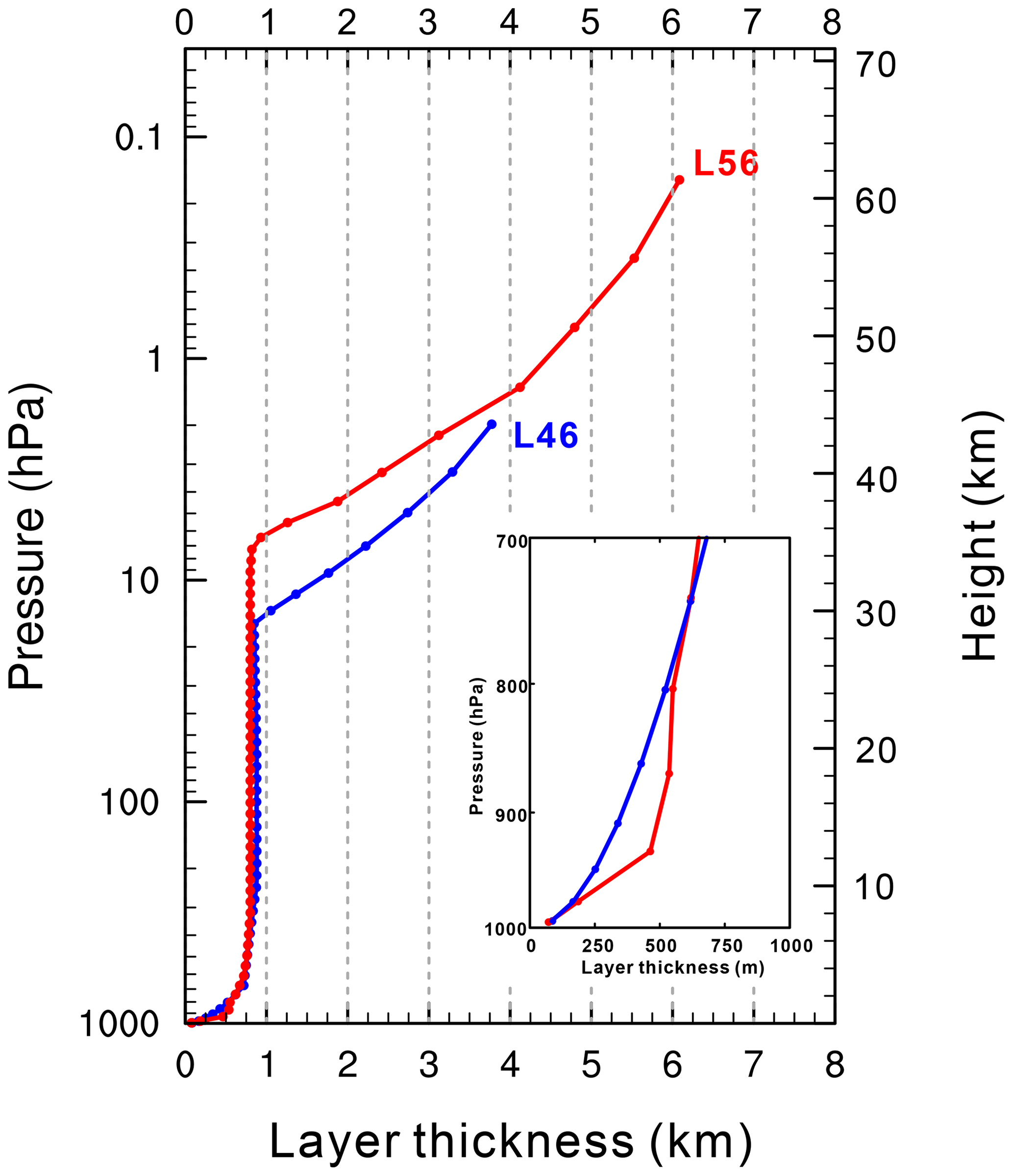
Figure 1 The profiles of layer thickness against height for 46 vertical layers in BCC-CSM2-MR (blue) and 56 vertical layers in BCC-CSM2-HR (red).

2.1 Atmosphere model

The atmospheric component of BCC-CSM2-MR is Beijing Climate Center Atmospheric General Circulation Model version 3 (BCC-AGCM3) at medium resolution (BCC-AGCM3-MR), with details being described in Wu et al. (2019b) and in a series of relevant publications (Wu et al., 2008, 2010; Wu, 2012; Wu et al., 2013; Lu et al., 2013; Wu et al., 2019a; Lu et al., 2020a; Wu et al., 2020a). The dynamical core in BCC-AGCM3-MR uses the spectral framework as described in Wu et al. (2008), in which an explicit time difference scheme is applied to vorticity equations, semi-implicit time difference schemes for divergence, temperature, and surface pressure equations, and a semi-Lagrangian tracer transport scheme is used for water vapour, liquid cloud water, and ice cloud water. The main model physics in BCC-AGCM3-MR was described in Wu et al. (2019b), which includes the modified scheme of deep convection suggested by Wu (2012), a new diagnostic scheme of cloud amount (Wu et al., 2019b), the shallow convection transport scheme of Hack (1994), the stratiform cloud microphysics following the framework of non-convective cloud processes in NCAR Community Atmosphere Model version 3 (CAM3, Collins et al., 2004) but with a different treatment for indirect effects of aerosols affecting clouds and precipitation, the radiative transfer parameterization that was originally implemented in CAM3, a modified boundary layer turbulence parameterization based on the eddy diffusivity approach (Holtslag and Boville, 1993), and a treatment of gravity waves that are generated by a variety of sources related to orography and convection (Lu et al., 2020a).

The atmospheric component in BCC-CSM2-HR is the newly developed version of BCC-AGCM3 with high resolution (BCC-AGCM3-HR). The main differences between BCC-AGCM3-HR and BCC-AGCM3-MR are listed in Table 1 and detailed in the following sub-sections. Actually, the high-resolution atmospheric component has incorporated a spatially varying divergence damping scheme, amelioration of Wu's deep convective scheme (Wu, 2012), and an integrated consideration for shallow convection and boundary layer processes.

2.1.1 Spatially varying divergence damping

The performance of a climate model is largely determined by complex motions at different spatio-temporal scales and interactions between them. Subgrid-scale motions are generally caused by high-frequency waves, and they can exert impacts on the computational stability, especially for a high-resolution model. Horizontal divergence damping is often needed to control numerical noise in weather forecast models and for numerical stability reasons (Dey, 1978; Bates et al., 1993; Whitehead et al., 2011).

In BCC-AGCM3-HR, second-order and fourth-order horizontal Laplacians (∇² and ∇⁴) are used to realize the damping operation on the divergence field D:

$$\begin{array}{}\text{(1)}& {\displaystyle \frac{\partial D}{\partial t}}=\mathrm{\dots }+k_{\mathrm{2}}{\mathrm{\nabla }}^{\mathrm{2}}D\end{array}$$

and

$$\begin{array}{}\text{(2)}& {\displaystyle \frac{\partial D}{\partial t}}=\mathrm{\dots }-k_{\mathrm{4}}{\mathrm{\nabla }}^{\mathrm{4}}D,\end{array}$$

where k₂ and k₄ express the damping coefficients for the second-order and fourth-order dissipation operators, respectively. They are generally set as constant parameters. The second-order damping is used for the top three layers and the fourth-order damping for other layers.

Whitehead et al. (2011) proposed a horizontal divergence damping scheme that works on a latitude–longitude grid by using a linear von Neumann analysis. Here, we extended their idea to the spectral dynamical core in our high-resolution model BCC-AGCM3-HR, and we use a second-order horizontal damping operator with a spatially varying damping coefficient. In order to express the grid spacing dependence of the dissipation, an additional term is introduced in Eqs. (1) and (2) as follows:

$$\begin{array}{}\text{(3)}& {\displaystyle \frac{\partial D}{\partial t}}=\mathrm{\dots }+k_{\mathrm{2}}{\mathrm{\nabla }}^{\mathrm{2}}D+k_v{\mathrm{\nabla }}^{\mathrm{2}}D\end{array}$$

and

$$\begin{array}{}\text{(4)}& {\displaystyle \frac{\partial D}{\partial t}}=\mathrm{\dots }-k_{\mathrm{4}}{\mathrm{\nabla }}^{\mathrm{4}}D+k_v{\mathrm{\nabla }}^{\mathrm{2}}D,\end{array}$$

where

$$\begin{array}{}\text{(5)}& k_v=C_s{\displaystyle \frac{\left[A_{\mathrm{E}}\mathrm{\Delta }\mathrm{\varnothing }\right]\cdot \left[A_{\mathrm{E}}\mathrm{\Delta }\mathit{\lambda }\right]}{\mathrm{\Delta }t}}.\end{array}$$

k_v is dependent on the time step Δt and grid spacing. A_E in Eq. (5) is the radius of the Earth. Δ∅ and Δλ stand for the latitudinal and longitudinal mesh sizes, respectively. The parameter C_s is designed to depend on vertical position as

$$\begin{array}{}\text{(6)}& C_s=C_{s\mathrm{0}}\max \langle \mathrm{1},\mathrm{8}\left\{\mathrm{1}+\tanh \left[\ln \left({\displaystyle \frac{p_{\mathrm{top}}}{p_k}}\right)\right]\right\}\rangle ,\end{array}$$

where C_s0 is a constant and related to model resolution, and p_top and p_k are the pressures at the top and the kth layers of the model, respectively. Equation (6) provides a rather flat vertical profile until the final two to three model levels, where the damping coefficient is increased rapidly by up to a factor of 8 (Whitehead et al., 2011). This dependence introduces a diffusive sponge layer near the model top to absorb rather than reflect outgoing gravity waves (Whitehead et al., 2011). Equation (5) implies the damping coefficient increases with latitude for BCC-AGCMs spectral grid. This spatially varying damping scheme can improve the atmospheric temperature simulation in the stratosphere, especially at polar areas of both hemispheres, which is possibly due to the more efficient damping of small-scale meridional waves as Whitehead et al. (2011) pointed out.

2.1.2 Deep convection

In BCC-AGCM3-MR, as well as in BCC-AGCM3-HR, a modified scheme of the deep cumulus convection developed by Wu (2012) is used (Wu et al., 2019b). It is characterized by the following points:

1. Deep convection is initiated at the level of maximum moist static energy above the boundary layer, and convection is triggered only when the boundary layer is unstable or there exists updraft velocity in the environment at the lifting level of convective cloud, and simultaneously there is positive convective available potential energy (CAPE).

2. A bulk cloud model is used to calculate the convective updraft with consideration of budgets for mass, dry static energy, moisture, cloud liquid water, and momentum, and the entrainment or detrainment amount for the updraft cloud parcel is determined according to the increase or decrease in updraft parcel mass with altitude.

3. The convective downdraft is assumed to be saturated and originated from the level of minimum environmental saturated equivalent potential temperature within the updraft cloud.

4. The closure scheme determines the mass flux at the base of convective cloud and depends on the decrease or increase in CAPE resulting from large-scale processes.

Along with increasing resolution in BCC-AGCM3-HR, the detrained cloud water can be transported to its adjacent grid boxes, which is accomplished in the dynamical core. Part of the horizontally transported cloud water is permitted to be transferred downward to the lower troposphere, and the amount of downward transferred water vapour is determined by the horizontally transported convective cloud water increment with time. These modifications of the deep convection scheme only in BCC-CSM2-HR are found to be in favour of improving the simulation of eastward propagation of MJO in the tropics, and their details will be presented in another paper.

2.1.3 Boundary layer turbulence

BCC-AGCM3-HR employs the University of Washington Moist Turbulence (UWMT) scheme as proposed in Bretherton and Park (2009) to replace the dry turbulence scheme of Holtslag and Boville (1993). The latter was used in BCC-AGCM3-MR. In UWMT, the first-order K diffusion is used to represent all turbulence values, by which the turbulent fluxes of a variable χ are written as

$$\begin{array}{}\text{(7)}& \stackrel{\mathrm{‾}}{w^{\prime }{\mathit{\chi }}^{\prime }}=-K_{\mathit{\chi }}{\displaystyle \frac{\partial \mathit{\chi }}{\partial z}}.\end{array}$$

The eddy diffusivity, Kχ, is calculated based on the turbulent kinetic energy e and proportional to the stability-corrected length scale L, given by

$$\begin{array}{}\text{(8)}& K_{\mathit{\chi }}=L\sqrt{e}.\end{array}$$

In the case of an entrainment layer at the top of convective boundary layers (BLs), the diffusivity is parameterized with

$$\begin{array}{}\text{(9)}& K_{\mathit{\chi }}=w_{\mathrm{e}}\mathrm{\Delta }{z}_{\mathrm{e}},\end{array}$$

where Δz_e is the thickness of the entrainment layer, and w_e is the entrainment rate which uses the expression in Nicholls and Turton (1986):

$$\begin{array}{}\text{(10)}& w_{\mathrm{e}}=A{\displaystyle \frac{w_{\ast }^{\mathrm{3}}}{\left(g{\mathrm{\Delta }}^{\mathrm{E}}{s}_{\mathrm{vl}}/s_{\mathrm{vl}}\right)\left(z_{\mathrm{t}}-z_{\mathrm{b}}\right)}}.\end{array}$$

Here, w_∗ is the convective velocity, z_t and z_b are the top and bottom heights of the entrainment layer, Δ^E denotes a jump across the entrainment layer, and s_vl is the liquid virtual static energy. A is a nondimensional entrainment efficiency, which is affected by evaporative cooling of mixtures of cloud-top and above-inversion air.

Compared to that of dry convective BLs over land, which is mainly forced by the surface heating, the structure of marine stratocumulus-topped BLs depends strongly on a dominant turbulence-generating mechanism resulting from both evaporative and radiative cooling at cloud top. The UWMT scheme aims to provide a more physical and realistic treatment of marine stratocumulus-topped BLs, and it has been demonstrated that the observed patterns of low-cloud amount with maxima in the subtropical stratocumulus decks can be well reproduced by UWMT in the Community Atmosphere Model (Park and Bretherton, 2009). The implementation of the UWMT scheme in BCC-AGCM3-HR aims to improve the simulation of the low-level clouds over subtropical eastern oceans, and these improvements are found to be critical to reducing the double-ITCZ bias of precipitation (Lu et al., 2020b).

2.1.4 Shallow convection

BCC-AGCM3-HR basically inherits the shallow convection parameterization used in BCC-AGCM3-MR, which is a stability-dependent mass-flux representation of moist convective processes with the use of a simple bulk three-level cloud model, as in Hack (1994). Specifically, in a vertically discrete model atmosphere where the level index k decreases upward and considering the case where layers k and k+1 are moist and adiabatically unstable, the Hack scheme assumes the existence of a non-entraining convective element with roots in level k+1, condensation and rain-out processes in level k, and limited detrainment in level k−1. By repeated application of this procedure from the bottom of the model to the top, the thermodynamic structure is locally stabilized.

The Hack shallow cumulus scheme can also be active in moist turbulent mixing, such as stratocumulus entrainment, which has different physical characteristics than cumulus convection. Shallow cumulus is usually regarded as a decoupled BL regime in which the vertical mixing processes do not achieve a single well-mixed layer, while the stratocumulus regime represents a well-mixed BL up to cloud top. The decoupling criterion to distinguish between the two regimes is of great importance for simulating the stratocumulus-to-cumulus transition (Bretherton and Wyant, 1997; Wood and Bretherton, 2004). A number of these decoupling criteria have been explored, such as static stability (Klein and Hartmann, 1993) and the buoyancy flux integral ratio (Turton and Nicholls, 1987). In light of its robustness, the stability criterion with a threshold of 17.5 K is introduced into the Hack scheme. The lower tropospheric stability (LTS) is defined as

$$\begin{array}{}\text{(11)}& \mathrm{LTS}={\mathit{\theta }}_{\mathrm{700}\mathrm{hPa}}-{\mathit{\theta }}_{\mathrm{sfc}},\end{array}$$

where θ_700 hPa and θ_sfc are potential temperatures at 700 hPa and at surface, respectively. In BCC-CSM2-HR, the modified Hack scheme is activated only in the decoupled BL regimes with LTS <17.5 K below 700 hPa to remove adiabatically moist instability, and the original Hack scheme (Hack, 1993) is still retained above 700 hPa to remove any local instability as long as the two adjacent model layers are moist and adiabatically unstable. This modification to the triggering of shallow convection is found to be very useful to improve the simulation of the ITCZ precipitation (Lu et al., 2020b).

2.2 Land surface model

BCC-AVIM2 is a comprehensive land surface model developed and maintained in BCC. Its previous version BCC-AVIM1 was used as the land component in BCC-CSM1.1m participating in CMIP5 (Wu et al., 2013), which includes major land surface biophysical processes treated similarly to in the Community Land Model version 3.0 (CLM3, Oleson et al., 2004) developed at the National Center for Atmospheric Research (NCAR) as well as plant physiological processes (Ji, 1995; Ji et al., 2008), with 10 layers for soil and up to 5 layers for snow. The land component in BCC-CSM2-MR and BCC-CSM2-HR is BCC-AVIM version 2 (Li et al., 2019). Updates in BCC-AVIM2 from its precedent version BCC-AVIM1 include a replacement of the water-only lake module by the common land model lake module (CoLM-lake) with a more realistic snow–ice–water–soil framework, a parameterization scheme for rice paddies added in the vegetation module, renewed parameterizations of snow cover fraction and snow surface albedo to accommodate the varied snow ageing effect during different stages of a snow season, a revised parameterization to calculate the threshold temperature to initiate freeze (thaw) of soil water (ice) rather than being fixed at 0 ^∘C in BCC-AVIM1, a prognostic phenology scheme for vegetation growth instead of empirically prescribed dates for leaf onset and fall, and a renewed scheme to depict solar radiation transfer through the vegetation canopy. Details of the updates are given in Li et al. (2019). BCC-AVIM2 is implemented in BCC-CSM2-MR and is identical to what is implemented in BCC-CSM2-HR, except for horizontal resolution (same as in their atmosphere component) and the corresponding sub-grid surface classification.

2.3 Ocean and sea-ice models

The ocean component of BCC-CSM2-MR is MOM4-L40, developed by the Geophysical Fluid Dynamics Laboratory (GFDL; Griffies et al., 2005). It has a nominal resolution of $\mathrm{1}{}^{\circ }\times \mathrm{1}{}^{\circ }$ with a tri-pole grid, and the actual resolution is from $\mathrm{1}/\mathrm{3}$^∘ latitude between 10^∘ S and 10^∘ N to 1^∘ at 60^∘ latitude. There are 40 levels in the vertical. More details of its implementation can be found in Wu et al. (2019b).

The ocean component of BCC-CSM2-HR is MOM5, also developed by GFDL (Griffies, 2012). The model is based on the hydrostatic primitive equations and uses the Boussinesq approximation. The model uses Arakawa B grid in the horizontal, with a globally uniform 0.25^∘ resolution. The quasi-horizontal rescaled height coordinate, namely the z^* vertical coordinate, is employed to enhance flexibility of model applications, which allows for the free surface to fluctuate to values as large as the local ocean depth. There are 50 levels in the vertical, with a resolution of 10 m in the upper ocean and 367 m at the bottom. The tracer advection scheme used in both the horizontal and vertical is the multi-dimensional piecewise parabolic method (MDPPM, Marshall et al., 1997), which is of higher order and more accurate (less dissipative).

MOM5 has a complete set of physical processes with advanced parameterization schemes. The effect of mesoscale eddies through the neutral diffusion scheme of Griffies et al. (1998) is not included in this work. The K-profile parameterization (KPP) is used to parameterize ocean surface boundary layer processes (Large et al., 1994). MOM5 uses the optical scheme of Manizza et al. (2005) to define the light attenuation exponentials. SeaWiFS chlorophyll a monthly climatology is used in the calculation of the attenuation of shortwave radiation entering the ocean layers with a maximum depth set at 200 m. The re-stratification effect of sub-mesoscale eddies in the ocean surface mixed layer are parameterized with the sub-mesoscale scheme of Fox-Kemper et al. (2008, 2011).

The sea-ice component of BCC-CSM2-HR and BCC-CSM2-MR is SIS4 (Winton, 2000) and SIS5 (Delworth et al., 2006), respectively, both developed by GFDL. Both SIS4 and SIS5 are the sea-ice component of MOM4 and MOM5, respectively, and have three vertical layers including one snow cover and two ice layers of equal thickness. They operate on the same oceanic grid of MOM4 in BCC-CSM2-MR and MOM5 in BCC-CSM2-HR, respectively. There are up to five categories of sea ice on each model grid for SIS4 and SI5 according to the thickness of sea ice, and the mutual transformation from one category to another are taken into account under thermodynamic conditions. Both SIS4 and SIS5 employ the scheme of Semtner (1976) for the vertical thermodynamics and contains full dynamics with internal ice forces calculated using an elastic–viscous–plastic rheology.

3 Experimental design and data used

3.1 Historical simulation

The principal simulation to be analysed is the CMIP6 historical run (hereafter referred to as historical) with prescribed forcings from 1850 to 2014 for BCC-CSM2-MR and from 1950 to 2014 for BCC-CSM2-HR. All historical forcings are from the CMIP6-recommended data (https://esgf-node.llnl.gov/search/input4mips/, last access: 1 April 2018) including (1) greenhouse gases concentrations such as CO₂, N₂O, CH₄, CFC11, and CFC12 with zonal-mean values and updated monthly; (2) annual means of total solar irradiance derived from the CMIP6 solar forcing; (3) stratospheric aerosols from volcanoes; (4) CMIP6-recommended tropospheric aerosol optical properties due to anthropogenic emissions that are formulated in terms of nine spatial plumes associated with different major anthropogenic source regions using version 2 of the Max Planck Institute Aerosol Climatology Simple Plume model (MACv2-SP, Stevens et al., 2017); (5) time-varying gridded ozone concentrations; and (6) yearly global gridded land-use forcing. In addition, aerosol masses based on CMIP5 (Taylor et al., 2012) are also used for the on-line calculation of cloud droplet effective radius in our models.

The historical simulation of BCC-CSM2-MR follows the requirement of CMIP6, with the preindustrial initial state obtained after a 500-year piControl simulation. It covers the whole period from 1850 to 2014 (Wu et al., 2019b). The simulation of BCC-CSM2-HR covers a shorter historical period from 1950 to 2014. Its initial state is the final state from a 50-year control simulation with fixed historical forcing of the year 1950, following the HighResMIP protocol. The control run itself is initiated from the states of individual components with their uncoupled mode. That is, the states of atmosphere and land are obtained from a 10-year AMIP run forced with monthly climatology of sea surface temperature (SST) and sea-ice concentration, while the states of ocean (MOM5) and sea ice (SIS5) are derived from a 1000-year forced run with a repeating annual cycle of monthly climatology of atmospheric state from the Coordinated Ocean-Ice Reference Experiment (CORE) dataset version 2 (Danabasoglu et al., 2014).

3.2 Data used for evaluations

We choose the same period of 1950–2014 from both BCC-CSM2-MR and BCC-CSM2-HR historical simulations to evaluate their performance against observation-based or reanalysis data.

The 1950–2014 monthly global 1^∘ × 1^∘ gridded surface temperature from the Hadley Centre–Climatic Research Unit (HadCRUT version 4.6.0.0, available at https://www.metoffice.gov.uk/hadobs/hadcrut4/, last access: 1 May 2019) is used to evaluate the global warming trend from BCC-CSM2-MR and BCC-CSM2-HR. HadCRUT (Morice et al., 2012) is a dataset combining land surface air temperature from the Climatic Research Unit (CRUTEM) and Hadley Centre Sea Ice and Sea Surface Temperature (HadISST). CRUTEM is derived from air temperatures near the land surface recorded at weather stations across the globe (Harris and Jones, 2017). HadISST contains global 1^∘ × 1^∘ sea-ice concentration and SST, including in situ measurements from ships and buoys (Rayner et al., 2003).

For the evaluation of present-day mean climate over the globe and major climate variabilities in the tropics, we choose the recent past 20 years of 1995–2014 as our reference period, which will be observed as close as possible for observation-based or reanalysis data, described as follows.

The 2001–2014 monthly global $\mathrm{1}{}^{\circ }\times \mathrm{1}{}^{\circ }$ gridded net radiations at the top of the atmosphere (TOA) from CERES-EBAF version 4.1 products (Loeb et al., 2018; available at https://asdc.larc.nasa.gov/project/CERES/CERES_EBAF_Edition4.1, last access: 1 May 2020) are used to evaluate the global energy budget in models. CERES-EBAF data are derived on the basis of satellite observation from CERES (Clouds and Earth's Radiant Energy System) and synthesized with EBAF (Energy Balanced and Filled) data. Satellite observation is a direct monitoring of the net radiation at TOA, and a primary source of data for estimating Earth's energy balance (Wielicki et al., 1996).

The 1995–2014 monthly global 0.25^∘ × 0.25^∘ gridded atmospheric temperature and wind from the fifth generation of ECMWF (the European Centre for Medium-Range Weather Forecasts) atmospheric reanalyses (ERA5, Hersbach and Dee, 2016) and the climatological data of global zonal mean temperature and wind above the 1 hPa level to 0.1 hPa at 5^∘ latitude interval from the COSPAR (Committee on Space Research) International Reference Atmosphere (CIRA86) are used to evaluate the vertical structure of atmospheric temperature and wind. The 1995–2014 monthly global gridded wind data from ERA5 are also used to evaluate the quasi-biennial oscillation (QBO) of the equatorial zonal wind between easterlies and westerlies in the tropical stratosphere. CIRA-86 (available at https://catalogue.ceda.ac.uk/uuid/4996e5b2f53ce0b1f2072adadaeda262, last access: 1 May 2020) includes a global climatology of zonal atmospheric temperature and velocity extending from pole to pole on a 5^∘ latitude grid and approximately 0–120 km at 2 km vertical resolution. It is derived from a combination of satellite, radiosonde, and ground-based measurements (Fleming et al., 1990).

The 1995–2014 monthly global observed precipitation at 2.5^∘ resolution is taken from the Global Precipitation Climatology Project (GPCP version 2.2; Adler et al., 2003) dataset and used to evaluate the global distribution of precipitation climatology.

The 2001–2014 quasi-global (60^∘ N–60^∘ S) 0.1^∘ × 0.1^∘ gridded half-hourly precipitation estimates of Global Precipitation Measurement (GPM) Integrated Multi-satellitE Retrievals for GPM (IMERG) products (available at https://gpm1.gesdisc.eosdis.nasa.gov/data/GPM_L3/GPM_3IMERGHH.06/, last access: 1 May 2020) are used to derive 3-hourly data and then to evaluate the spectrum of precipitation intensity. IMERG uses inter-calibrated estimates from the international constellation of precipitation-relevant satellites and other data sources, including surface precipitation gauge analyses (Huffman et al., 2019).

Two datasets (CRUTEM and HadISST) of the 1995–2014 monthly global 1^∘ × 1^∘ gridded surface temperature for the land (Jones et al., 2012) and ocean (Rayner et al., 2003) and gridded sea-ice concentration are used to evaluate the model biases of land and ocean temperatures as well as sea-ice cover. For the assessment of the ENSO cycle variation, a longer period of 1950–2014 is used from the global monthly HadISST dataset.

The 1995 to 2014 daily global 0.25^∘ × 0.25^∘ wind from ERA5, daily global 2.5^∘ × 2.5^∘ outgoing longwave radiation (OLR) from NOAA (Liebmann and Smith, 1996), and daily global 2.5^∘ × 2.5^∘ precipitation from GPCP (Adler et al., 2003) are used to diagnose the Madden–Julian Oscillation (MJO), which is the dominant mode of sub-seasonal variability in the tropical troposphere (Madden and Julian, 1971). All the data firstly undergo the 20–100 d band-pass filter. An analysis of multivariate empirical orthogonal functions (EOFs) and principal components (PCs) is then performed on intra-seasonal OLR, 850, and 200 hPa zonal wind anomalies averaged over 10^∘ S–10^∘ N. Eight MJO phases defined by the inverse tangent of the ratio of PC2 to PC1 as in Wheeler and Hendon (2004) are also reconstructed.

The 1995–2014 6-hourly tropical cyclone observations from International Best Track Archive for Climate Stewardship (IBTrACS; Knapp et al., 2010) provide information of all tropical cyclones, including latitude–longitude position, minimum central pressure, and maximum sustained winds (instantaneous values) at a time frequency of every 6 h. We use the multiple criteria reported by Murakami (2014) to detect TCs with 6-hourly outputs from models (instantaneous values from BCC-CSM2-HR, but accumulated values from BCC-CSM2-MR). (1) The maximum of relative vorticity of a TC-like vortex at 850 hPa exceeds 15 × 10⁻⁵ s⁻¹ (a threshold that can vary from 1 × 10⁻⁵ to 15 × 10⁻⁵ s⁻¹ as a function of resolution (Murakami, 2014). (2) The warm-core above the TC-like vortex, which is presented as the sum of the air temperature deviations (subtracting the maximum temperature from the mean temperature within the TC-like vortex centre for an area of 10^∘ × 10^∘) at 300, 500 and 700 hPa, exceeds 0.8 K, a threshold falling in the range 0.6–1.0 K that is recommended in Murakami (2014). (3) the maximum wind speed at 850 hPa is higher than that at 300 hPa. (4) The maximum wind speed at 10 m within the TC-like vortex centre for an area of 3^∘ × 3^∘ grid is higher than 10 m s⁻¹. (5) The genesis position of the TC-like vortex is over the ocean. (6) The duration of the TC-like vortex that satisfied above conditions exceeds 48 h.

4 Results

Data analysis and visualization are generally on the original or native grid of observation and models. An exception is the assessment of models' biases in contrast to observation. In this case, simulations are re-gridded onto the grid of corresponding observation.

4.1 Global mean surface air temperature variations from 1950 to 2014

The historical simulation from 1950 to 2014 allows us to evaluate the ability of models to reproduce the global warming of near-surface temperature. Figure 2 presents global-mean surface air temperature evolutions for HadCRUT4 data and the two BCC models, in which the climatological mean is calculated for the reference period 1961–1990 and removed from the time series to better reveal long-term trends. The interannual variability of both simulations is qualitatively comparable to that observed, and the correlation coefficients reach 0.84 in both models. A remarkable feature in Fig. 2 is the presence of a global warming hiatus or pause for the period from 1998 to 2013 when the observed global surface air temperature warming slowed down. It is interesting that both models reproduce a hiatus, from 2002 to 2010 in BCC-CSM2-MR and from 2004 to 2012 in BCC-CSM2-HR. This warming hiatus is a hot topic (e.g. Fyfe et al., 2016; Medhaug et al., 2017; Wu et al., 2019a), largely debated in the scientific research community. The reason why the BCC models simulate the recent global warming hiatus is beyond the scope of this paper and will be explored in other works.

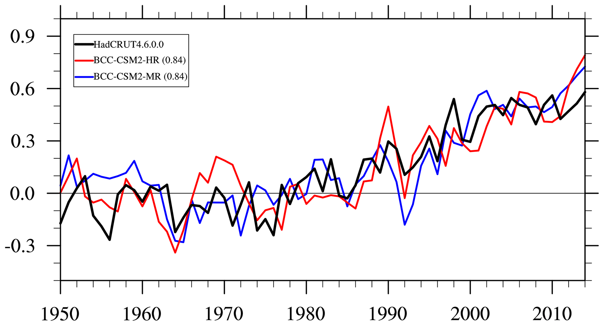
Figure 2 Time series of anomalies in the global mean surface air temperature from 1950 to 2014. The reference climate to deduce anomalies is for each individual curve from 1961 to 1990. The numbers in the parentheses denote the correlation coefficient of 11-year smoothed simulations with HadCRUT4.6.0.0 (Morice et al., 2012) observations.

4.2 Global energy budget

It is to be noted that only the period 2001–2014 is available for CERES-EBAF. For the consistency of comparison, we also shortened data from models and kept the same time interval as in CERES-EBAF. As shown in Table 2, the globally averaged TOA net energy is 2.12 ± 0.40 W m⁻² in BCC-CSM2-MR and 1.51 ± 0.57 W m⁻² in BCC-CSM2-HR for the same period from 2001 to 2014. The energy equilibrium of the whole Earth system in BCC-CSM2-HR is slightly improved. The TOA shortwave and longwave components for clear sky in BCC-CSM2-HR are also much closer to CERES-EBAF than in BCC-CSM2-MR. We noted that the TOA shortwave and longwave components for all sky in BCC-CSM2-HR are lower than CERES-EBAF data and are not improved from BCC-CSM2-MR. This is related to cloud radiative forcing. Clouds constitute a major modulator of the radiative transfer in the atmosphere, and their radiative properties exert strong impacts on the equilibrium and variation of the radiative budget at TOA. The globally averaged shortwave cloud radiative forcing in BCC-CSM2-HR is slightly stronger than that in CERES-EBAF (−47.16 ± 0.24 W m⁻²), about 3 W m⁻² of the cooling effect, and the globally averaged longwave cloud radiative forcing in BCC-CSM2-HR is also stronger than the CERES-EBAF data (25.99 ± 0.25 W m⁻²) near 2 W m⁻² of warming effect (biases). The globally averaged shortwave and longwave cloud radiative forcing in BCC-CSM2-MR are much closer to CERES-EBAF.

Table 2 Energy balance and cloud radiative forcing at the top of the atmosphere (TOA) in the models in contrast to CERES-EBAF observations. Units: W m⁻².

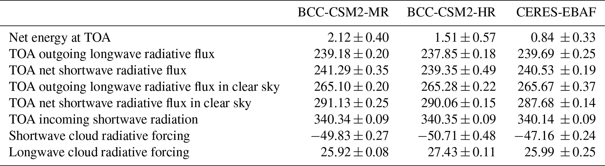
Notes: mean value and standard deviation are calculated from 2001–2014 yearly global means of the simulations for BCC-CSM2-MR, BCC-CSM2-HR, and the CERES-EBAF Ed4.1 dataset.

The obvious biases of the model in contrast to CERES-EBAF are mainly located at the mid-latitudes and subtropics. Figure 3 shows the annual and zonal mean of shortwave, longwave, and net cloud radiative forcing for the two model versions and observations. The longwave and net cloud radiative forcing are overall consistent with CERES-EBAF at most latitudes. In the mid-latitudes of both the hemispheres, the shortwave cloud radiative forcing from BCC-CSM2-HR is much closer to CERES-EBAF than that from BCC-CSM2-MR. But at low latitudes between 30^∘ S and 30^∘ N, BCC-CSM2-HR simulates excessive cloud shortwave radiative forcing which mainly comes from evident biases over the eastern tropical Pacific and tropical Atlantic oceans (Fig. 4). These biases are possibly attributable to new treatments for boundary layer processes.

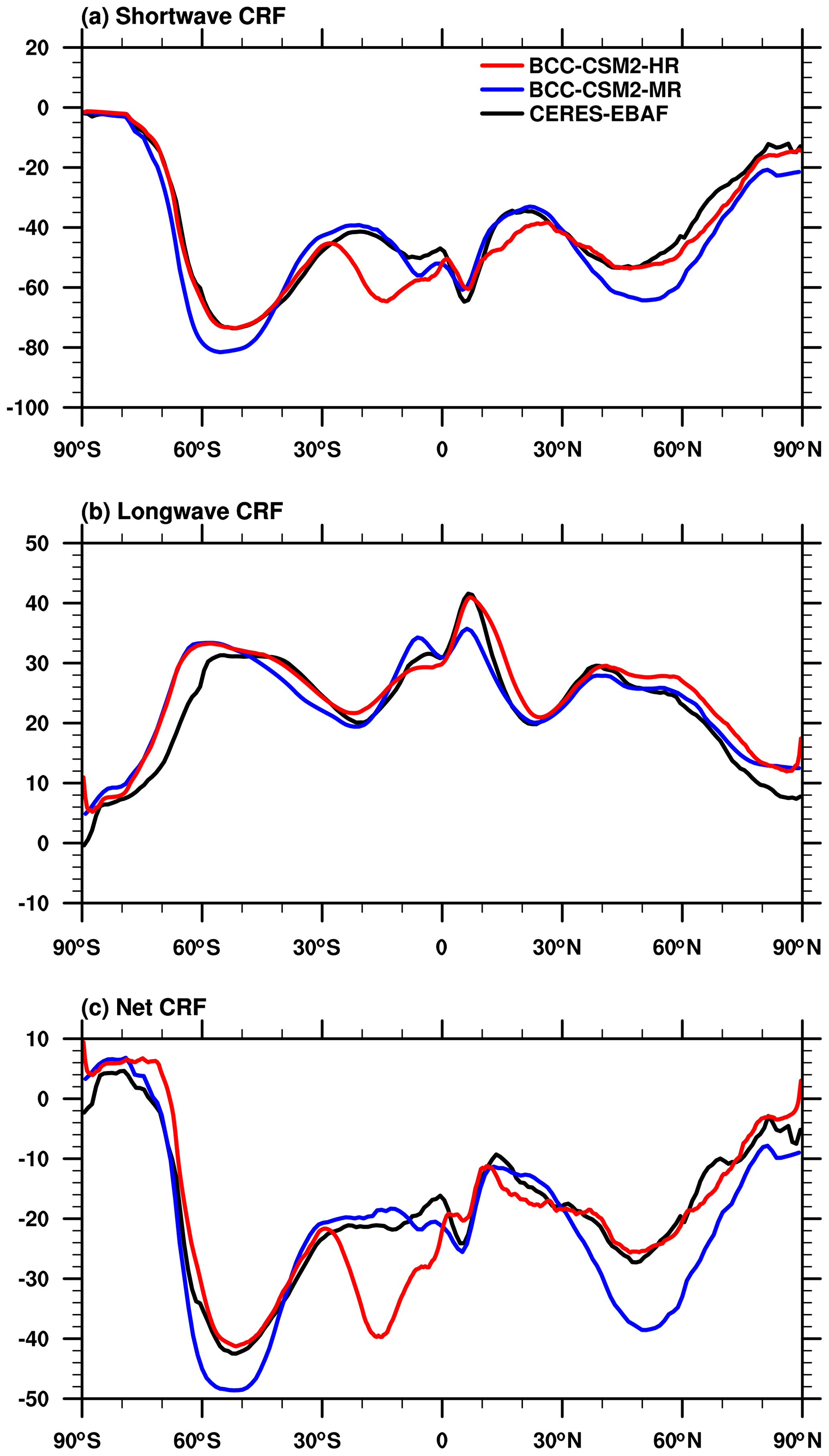
Figure 3 Zonal averages of (a) shortwave, (b) longwave, and (c) net cloud radiative forcing (CRF, in W m⁻²) for the historical simulations (2001–2014) of BCC-CSM2-MR (blue lines) and BCC-CSM2-HR (red lines), compared to the 2001–2014 CERES-EBAF observations (black lines).

Figure 4 The 2001–2014 averaged annual-mean shortwave cloud radiative forcing for (a) the CERES-EBAF observations, the historical simulations from (b) BCC-CSM2-MR and (c) BCC-CSM2-HR and their biases (d, e) against CERES-EBAF data. Units: W m⁻².

4.3 Present-day mean climate

4.3.1 Vertical structure of the atmospheric temperature and wind

Figure 5 presents zonally averaged vertical profiles of air temperature and zonal wind for December–January–February (DJF) and June–July–August (JJA) as simulated by BCC-CSM2-MR and BCC-CSM2-HR, in contrast to the ERA5 reanalysis below the 1 hPa level (Hersbach and Dee, 2016) and climatological values above the 1 hPa level from CIRA86 (Fleming et al., 1990). The observed vertical profile of atmospheric temperature shows a clear structure of stratification, with an evident seasonal transition. In DJF, it is characterized as cool layers over broader latitudes spanning the transition from troposphere to stratosphere over the Northern Hemisphere, and warm layers spanning from the top of the stratosphere to the mesosphere over the Southern Hemisphere. Those different vertical structures in both hemispheres during DJF are almost reversed in JJA. BCC-CSM2-HR is capable of capturing the structure of the upper stratosphere and the transition to mesosphere while BCC-CSM2-MR cannot.

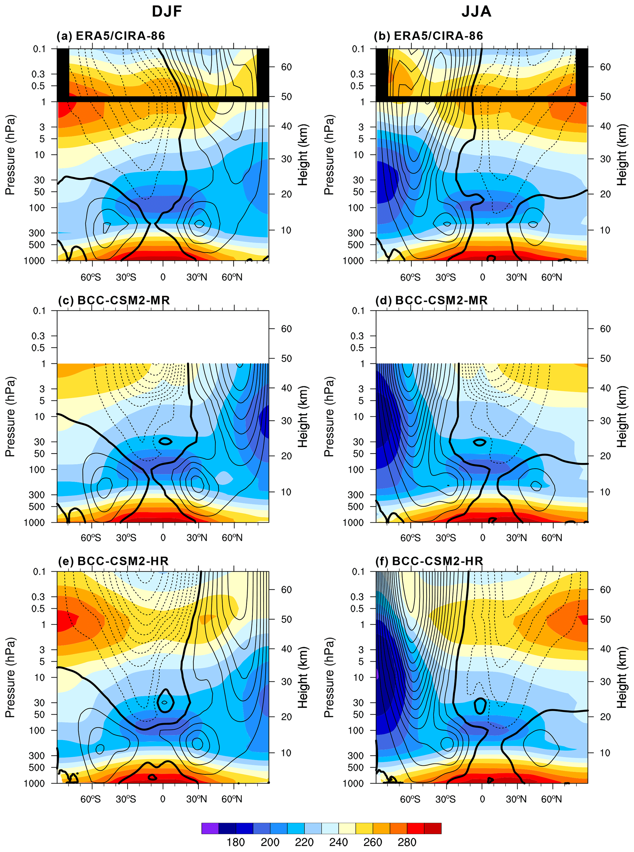
Figure 5 The zonal means of temperature (colours; K) and zonal wind (contours; m s⁻¹) averaged for December–January–February (a, c, e) and June–July–August (b, d, f) from 1995 to 2014 for (a, b) ERA5/CIRA86, (c, d) BCC-CSM2-MR, and (e, f) BCC-CSM2-HR. Positive (negative) zonal winds are plotted with solid (dashed) lines with a contour interval of 10 m s⁻¹. Thick contour lines denote zero zonal wind speed. In (a) and (b), the values above 1 hPa from the COSPAR International Reference Atmosphere (CIRA86, Fleming et al., 1990) and below 1 hPa from the ERA5 reanalysis.

Figure 6 shows biases of the zonally averaged annual air temperature, relative to ERA5. Only model data from 5 to 1000 hPa are evaluated as there are spare station-based observations above 5 hPa and it is generally recognized that most of the stations do not reach their best-practice altitude of 5 hPa (https://gcos.wmo.int/en/atmospheric-observation-panel-climate, last access: 1 May 2020). Temperature biases in the lower to middle troposphere are relatively small, about −2 to 2 K in BCC-CSM2-MR and −1 to 1 K in BCC-CSM2-HR at most latitudes, except in the southern polar region where temperature below 700 hPa are extrapolated values for ERA5 observation and models. The two models BCC-CSM2-MR and BCC-CSM2-HR have a cold bias of air temperature that appears near the tropopause and extends to the stratosphere in the subpolar and polar regions. There is also a thicker layer of warm biases in the lower stratosphere over the tropics and mid-latitudes. Those temperature biases are not really reduced in BCC-CSM2-HR with a higher horizontal resolution. The cold bias in the troposphere was also reported in many CMIP5 models (see Charlton-Perez et al., 2013; Tian et al., 2013),

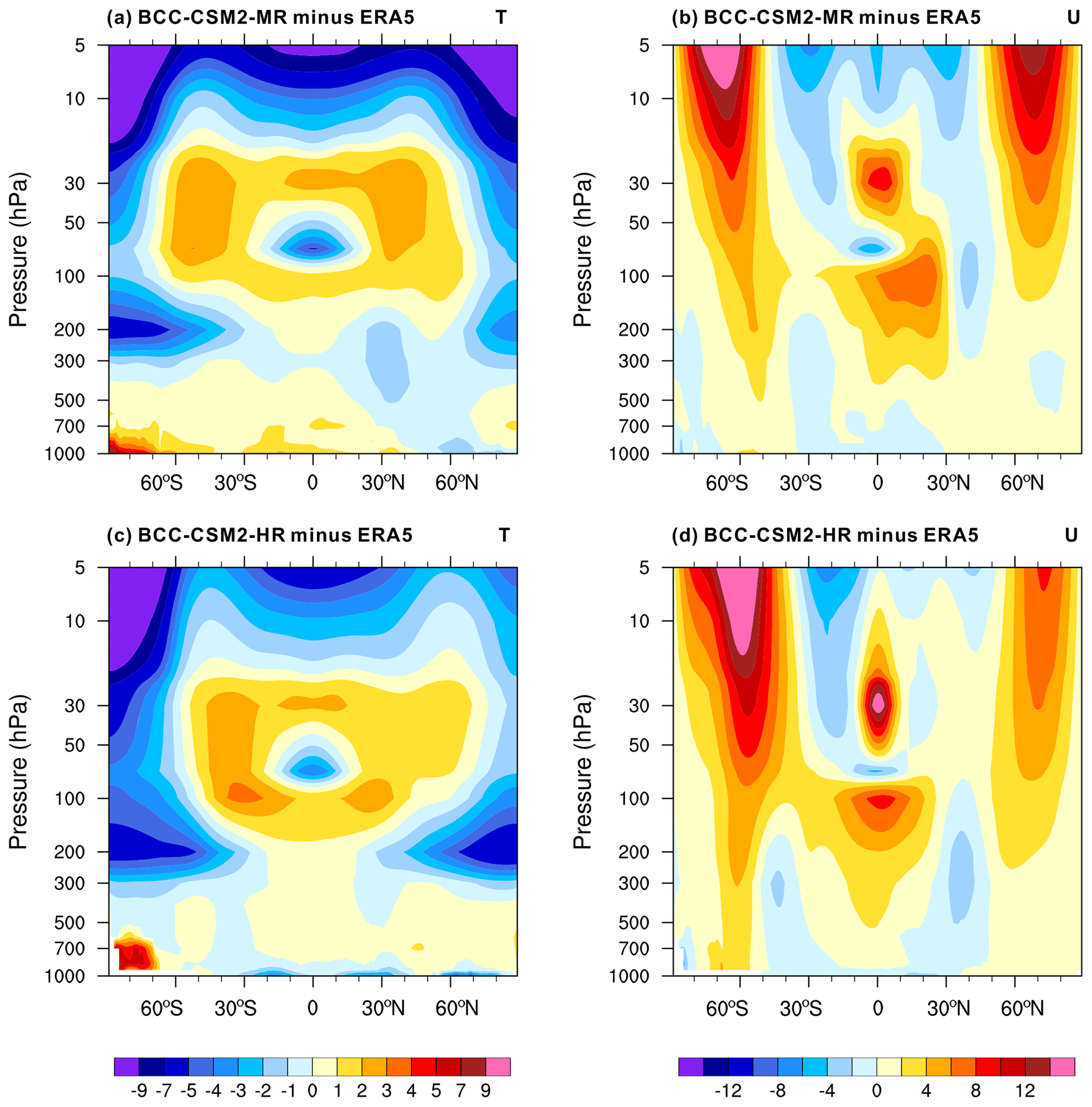
Figure 6 Zonally averaged annual mean temperature biases (a, c, in K) and zonal wind biases (b, d, in m s⁻¹) averaged for the period from 1995 to 2014 for (a, b) BCC-CSM2-MR and (c, d) BCC-CSM2-HR, with respect to the ERA5 reanalysis data.

As shown in Fig. 5, the basic pattern of vertical structures of westerly and easterly zones and their changes in DJF and JJA are generally well simulated by BCC-CSM2-MR and BCC-CSM2-HR. Both models have westerly wind biases of annual means that are located in the upper troposphere and stratosphere near 60^∘ S and 60^∘ N (Fig. 6b and d) and reflect the meridional structure of temperature biases (Fig. 6a and c) in accordance with the temperature–wind relationship.

4.3.2 Precipitation

Figure 7 shows the spatial distribution of DJF and JJA mean precipitation for BCC-CSM2-MR and BCC-CSM2-HR, compared to GPCP data. The two versions of BCC-CSMs were both able to reproduce the global observed precipitation patterns, and there is an evident improvement in the high-resolution model (BCC-CSM2-HR). Improvements are particularly clear in the Pacific, Indian, and Atlantic oceans. The double-ITCZ issue is one of the most significant biases that persists in many climate models (e.g. Hwang and Frierson, 2013; Li and Xie, 2014). It exists in BCC-CSM2-MR, with excessive precipitation in the South Pacific Convergence Zone (SPCZ). This bias almost disappears in BCC-CSM2-HR. As shown in Fig. 8, there is too much precipitation along the southern intertropical convergence zone (ITCZ) in BCC-CSM2-MR, which is mainly caused by excessive precipitation in the southern intertropical zone in DJF. This systematic bias is evidently reduced in BCC-CSM2-HR, especially with weakened precipitation in the South Pacific Convergence Zone (SPCZ). The improvement of SPCZ precipitation in BCC-CSM2-HR might be attributed to the implementation of the UWMT scheme which improved the simulation of low-level clouds over the tropical eastern South Pacific (Lu et al., 2020b) and reduced warm biases there (Fig. 10c). But the intensity of precipitation in the northern intertropical convergence zone in BCC-CSM2-HR is stronger than that from GPCP, which is partly attributed to the excessive precipitation in the tropical oceans, especially in the eastern tropical North Pacific (Fig. 7e). A strong negative bias of JJA precipitation over the Amazon region exists in the two models. In Fig. 7f, we also noted that the amount of JJA precipitation in the east of the Philippines and near the Pacific warm pool is worsened, since it is smaller in BCC-CSM2-HR than in BCC-CSM2-MR and GPCP data. This bias of lacking precipitation in BCC-CSM2-HR may partly be caused by a cold-SST bias over the western Pacific warm pool (Fig. 10c).

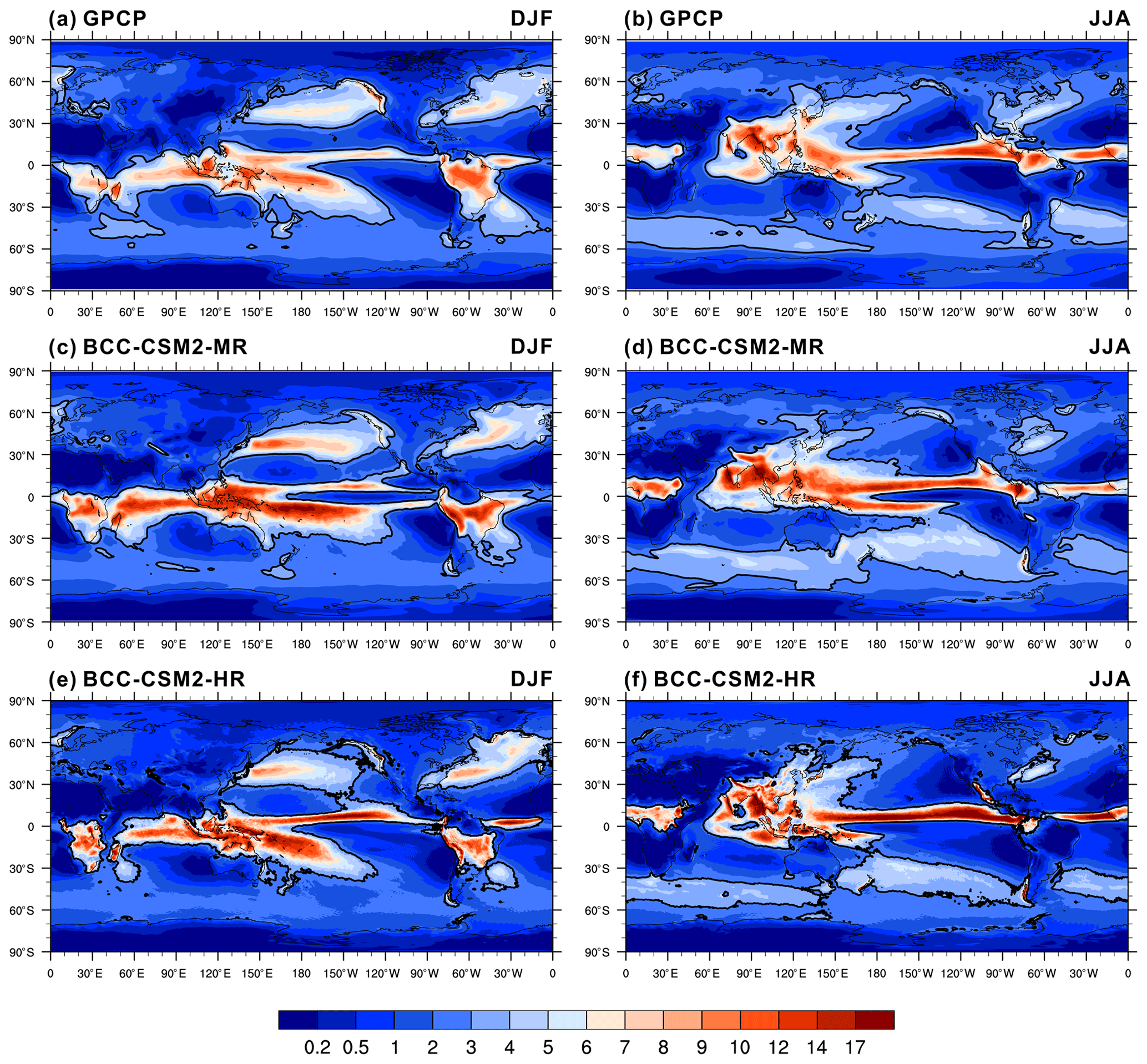
Figure 7 The 1995–2014 averaged mean precipitation rate of December–January–February (a, c, e) and June–July–August (b, d, f) for (a, b) GPCP observations, (c, d) BCC-CSM2-MR, and (e, f) BCC-CSM2-HR. Units: mm d⁻¹. The 3 mm d⁻¹ contour line is in bold as a reference to facilitate the visual inspection.

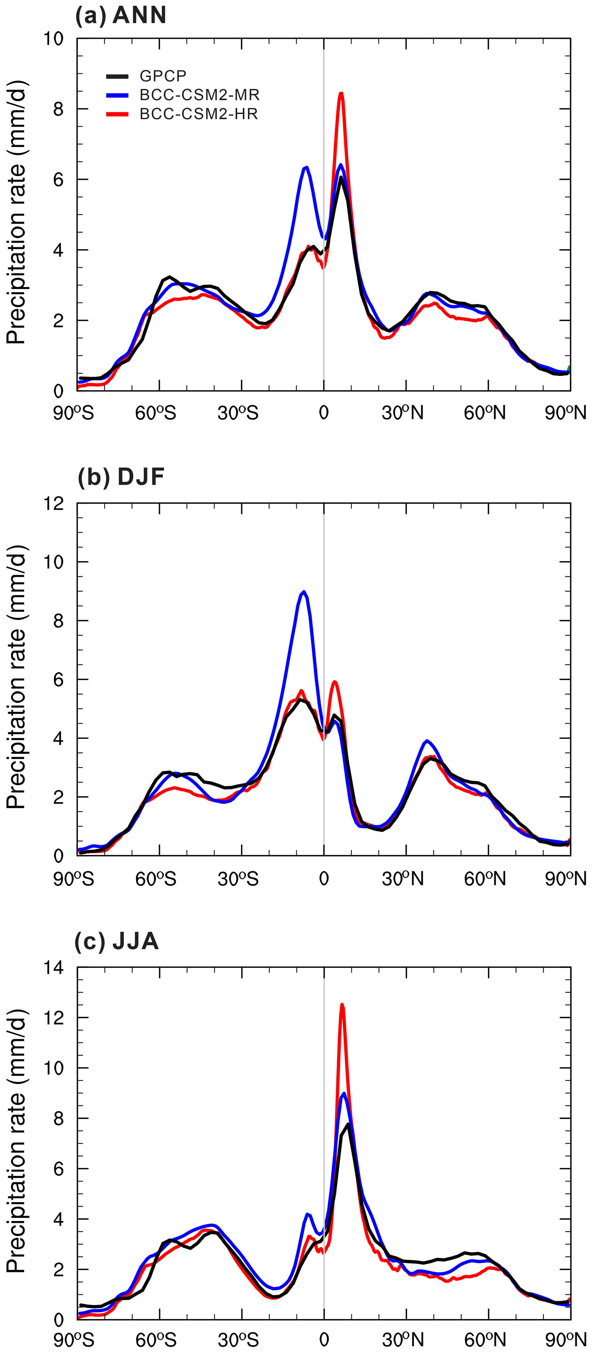
Figure 8 The 1995–2014 averaged zonal mean precipitation rate (mm d⁻¹) for (a) the annual mean, (b) December–January–February, and (c) June–July–August. The solid black lines denote GPCP data, and the colour lines show BCC-CSM2-MR (blue) and BCC-CSM2-HR (red) simulations. Units: mm d⁻¹.

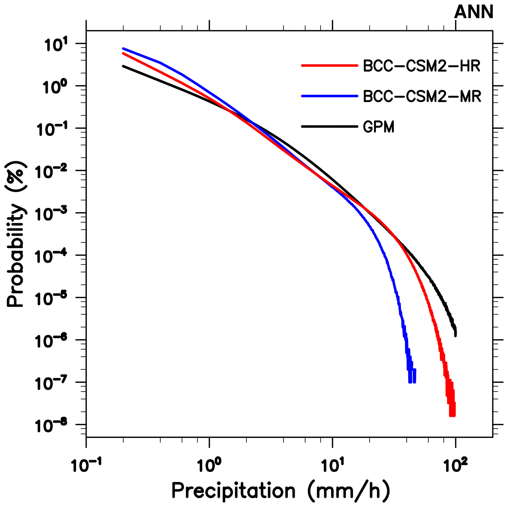
Figure 9 The probability density of 3-hourly precipitation between 40^∘ S and 40^∘ N and during the period from 2001 to 2014, as a function of precipitation intensity with intervals of 1 mm h⁻¹, for IMERG precipitation (black line), BCC-CSM2-MR (blue line), and BCC-CSM2-HR (red line). The two simulations were re-gridded to the grid of IMERG before processing.

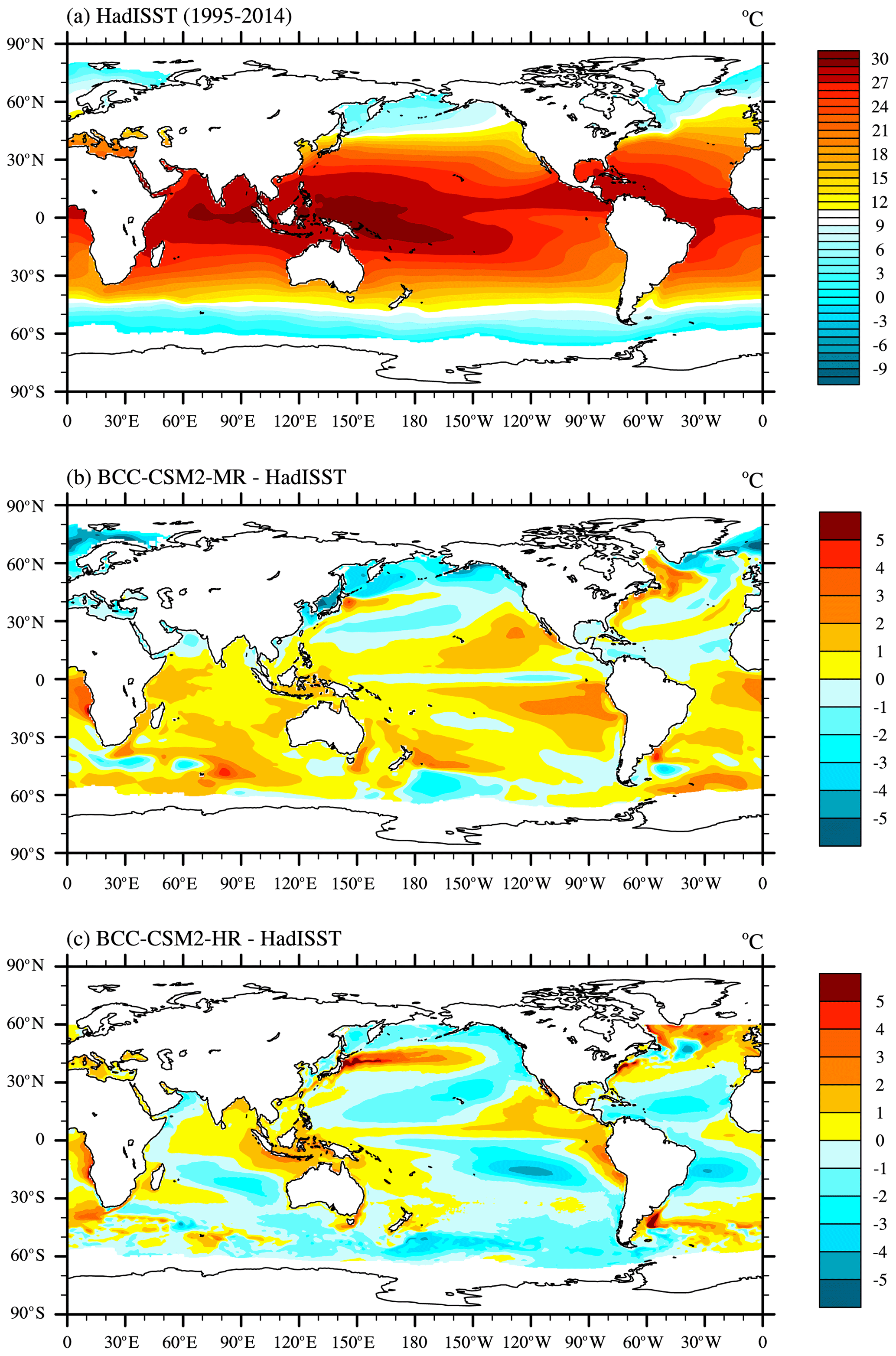
Figure 10 The global distributions of the 1995–2014 annual mean sea surface temperature for (a) the observations from HadISST, and the simulation biases in (b) BCC-CSM2-MR and (c) BCC-CSM2-HR.

Figure 9 shows the probability density of 3-hourly precipitation between 40^∘ S and 40^∘ N as a function of precipitation intensity with intervals of 1 mm h⁻¹. The frequency of light rainfall events, smaller than 1 mm h⁻¹, in BCC-CSM2-MR is higher than in IMERG. But strong precipitation events exceeding 10 mm h⁻¹ are clearly insufficient. This is a common bias in many global climate models, raising concerns for any studies on precipitation extremes. Compared to BCC-CSM2-MR, BCC-CSM2-HR with resolution increased shows substantial improvements for its precipitation spectrum: reduced light rainfall and enhanced heavy rainfall events. The spectral distribution of precipitation in BCC-CSM2-HR is much closer to IMERG.

4.3.3 SST

Figure 10 shows a spatial-distribution map of the 1995–2014 annual mean SST for HadISST and the biases for BCC-CSM2-MR and BCC-CSM2-HR relative to HadISST. BCC-CSM2-MR is generally warmer, while BCC-CSM2-HR is colder than what was observed. A warm SST bias in BCC-CSM2-MR spreads throughout most oceans, except the North Pacific and North Atlantic. Such warm biases do not appear in BCC-CSM2-HR, and the cold SST biases in the eastern subtropical South Pacific are possibly attributable to excessive clouds there, also manifested by strong cloud shortwave radiative forcing (Fig. 4e). The warm biases in the eastern tropical ocean basins in BCC-CSM2-MR are associated with a deficit of stratiform low-level clouds, a common and systematic bias for many climate models (Richter, 2015). The cold biases there in BCC-CSM2-HR, similarly, are associated with too much low cloud, except over the tropical North Pacific. We also noted a belt of warm SST biases in the Kuroshio extension and in the North Atlantic in both models (Fig. 10b and c), especially in the high-resolution model. This bias may be partly a result of the coarse resolution of HadISST data used, as SST near the Kuroshio shows strong temperature gradients with filamentous structures (Shi and Wang, 2020).

4.3.4 Land–surface air temperature

Figure 11 shows the simulation biases of annual mean land–surface air temperature from BCC-CSM2-MR and BCC-CSM2-HR. The near-surface air temperature over land in BCC-CSM2-MR is generally colder than that in the CRUTEM observations, particularly exhibiting severe cold biases in northern Europe. As there are no physical (but only resolution) changes in the land modelling component in the two models, the systematic biases of near-surface air temperature over land are very similar to each other. Increasing atmospheric resolution in BCC-CSM2-HR does not seem to show amelioration, and the surface air temperatures in BCC-CSM2-HR exhibit rather similar patterns to those in BCC-CSM2-MR with biases of −2 to 2 K in most land regions between 50^∘ N and 50^∘ S compared to CRU data.

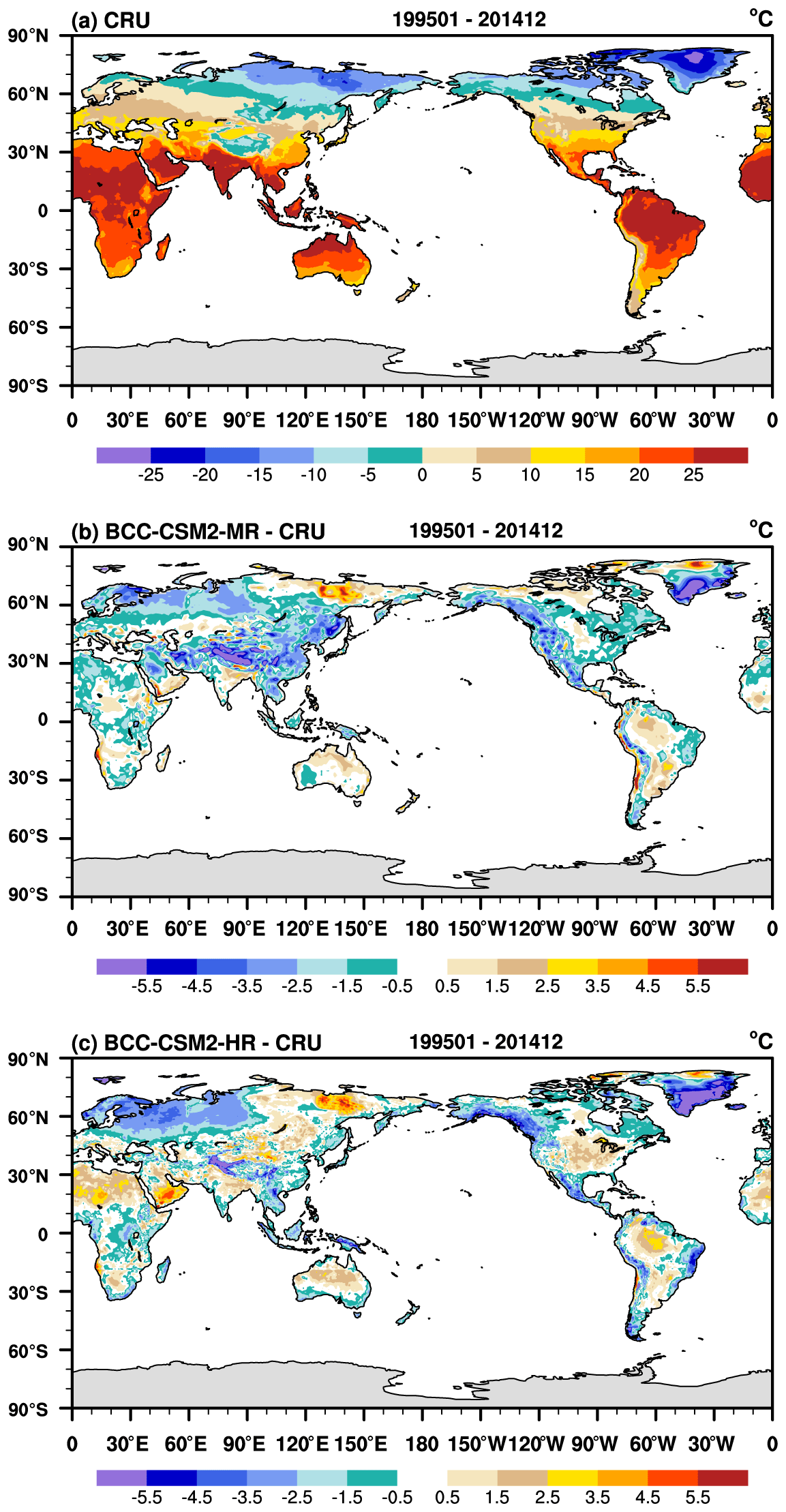
Figure 11 The 1995–2014 averaged global land–surface air temperature for (a) CRUTEM observations, and simulation biases in (b) BCC-CSM2-MR and (c) BCC-CSM2-HR.

4.3.5 Sea ice

Figure 12 shows the annual mean sea-ice concentration simulated by BCC-CSM2-MR and BCC-CSM2-HR over the period 1995–2014, compared to HadISST observation data. The simulated geographic distribution of sea ice in the Arctic is overall realistic, except that the sea-ice concentration in the Atlantic is slightly overestimated in both models. This overestimation of sea ice possibly has a consequence for the severe cold biases of surface air temperature in northern Europe (Fig. 11). In the Antarctic, sea-ice concentration simulated by BCC-CSM2-MR is smaller than that in HadISST data, especially from 60^∘ W to 60^∘ E in the subpolar region where the simulated SST is warmer compared to HadISST data (Fig. 10b). Those deficiencies in BCC-CSM2-MR (Fig. 12e) are largely reduced in BCC-CSM2-HR (Fig. 12f).

Figure 12 The spatial distribution of annual mean sea-ice concentration from BCC-CSM2-MR and BCC-CSM2-HR in contrast to the observations from the Hadley Centre Sea Ice dataset from 1995 to 2014.

Figure 13 shows the monthly sea-ice covers for the Arctic and Antarctic from BCC-CSM2-MR and BCC-CSM2-HR. HadISST observations show that the Arctic sea-ice cover reaches a minimum extent of 6.9 × 10⁶ km² in September and rises to a maximum extent of 16.0 × 10⁶ km² in March, and the Antarctic sea-ice cover reaches a minimum extent in February and a maximum extent in September. The seasonal cycle amplitude and phase of sea-ice area are well captured by the two models, and their biases are mostly smaller than 1 × 10⁶ km² compared to HadISST observations. We note that the extents of the Arctic sea ice for each month in BCC-CSM2-MR are slightly but systematically smaller than HadISST, and in the Antarctic are smaller in February and March but larger in other months than HadISST. BCC-CSM2-HR slightly overestimated sea-ice concentration by about 1 × 10⁶ km² in both hemispheres with reference to HadISST.

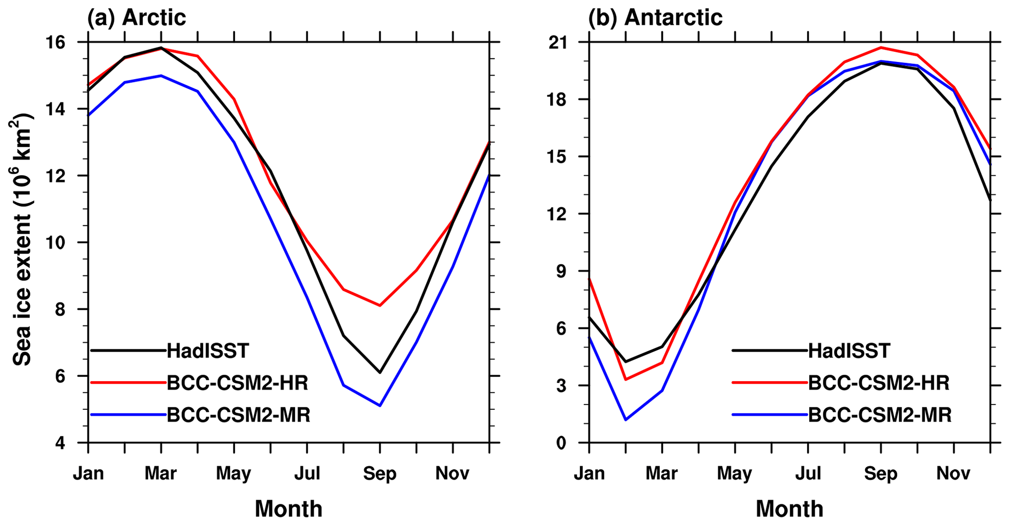
Figure 13 The mean (1995–2014) seasonal cycle of sea-ice extent (with a sea-ice concentration of at least 15 %) in (a) the Northern Hemisphere and (b) the Southern Hemisphere for the observations from the Hadley Centre Sea Ice and Sea Surface Temperature dataset (black lines) and the simulations from BCC-CSM2-MR (blue lines) and BCC-CSM2-HR (red lines).

4.4 Variabilities in the tropics

The tropical cyclone (TC), also known as typhoon or hurricane, is among the most destructive weather phenomena. The Madden–Julian Oscillation (MJO) is the dominant mode of sub-seasonal variability in the tropical troposphere (Madden and Julian, 1971), and the quasi-biennial oscillation (QBO) is a quasi-periodic oscillation of the equatorial zonal wind between easterlies and westerlies in the tropical stratosphere. TC, MJO, and QBO are very important variabilities in the tropics, with consequences for global weather and climate.

4.4.1 Tropical cyclones

In Fig. 14, we evaluate the average TC frequency over 20 years (1995–2014) from BCC-CSM2-MR and BCC-CSM2-HR, in contrast to the climatology of 1995–2014 observations from International Best Track Archive for Climate Stewardship (IBTrACS; Knapp et al., 2010). It is clear that TC activity is increased with resolution enhanced. The averaged total global TC numbers per year are 49.6 in BCC-CSM2-MR and 94.4 in BCC-CSM2-HR, and the global TC numbers in BCC-CSM2-HR are much closer to the IBTrACS observation (90.2). The global TC number is slightly influenced by the threshold (15 × 10⁻⁵ s⁻¹ in Fig. 14) of relative vorticity at 850 hPa used to detect TC. If this threshold gets looser to 5 × 10⁻⁵ s⁻¹, the averaged total global TC numbers per year in BCC-CSM2-MR and BCC-CSM2-HR would enhance to 55.9 and 101.5 (not shown), respectively. The low TC number in BCC-CSM2-MR is furthermore explained by the fact that its 6-hourly data used to detect TC are averaged values in the 6 h interval, while instantaneous values would be more appropriate as in IBTrACS and BCC-CSM2-HR. Spatially, BCC-CSM2-HR generates excess TC activity in the eastern North Pacific, northern Indian Ocean, and Southern Hemisphere. But both models severely underestimate TC activity in the North Atlantic and in the Caribbean Sea. The general overestimation of TC activity in the eastern North Pacific and the opposite in the North Atlantic in BCC-CSM2-HR may be related to the warmer SST in the eastern tropical North Pacific and colder SST in the tropical Atlantic in contrast to HadISST data (Fig. 10c), but other factors such as the entrainment in the parameterization of convection (Zhao et al., 2012) and air–sea coupling (Li and Sriver, 2018) may also have an influence. The study of Li and Sriver (2018) showed that ocean coupling influences simulated TC frequency, geographical distributions, and storm intensity, and TC tracks are relatively sparse in the coupled simulations compared to un-coupled simulations.

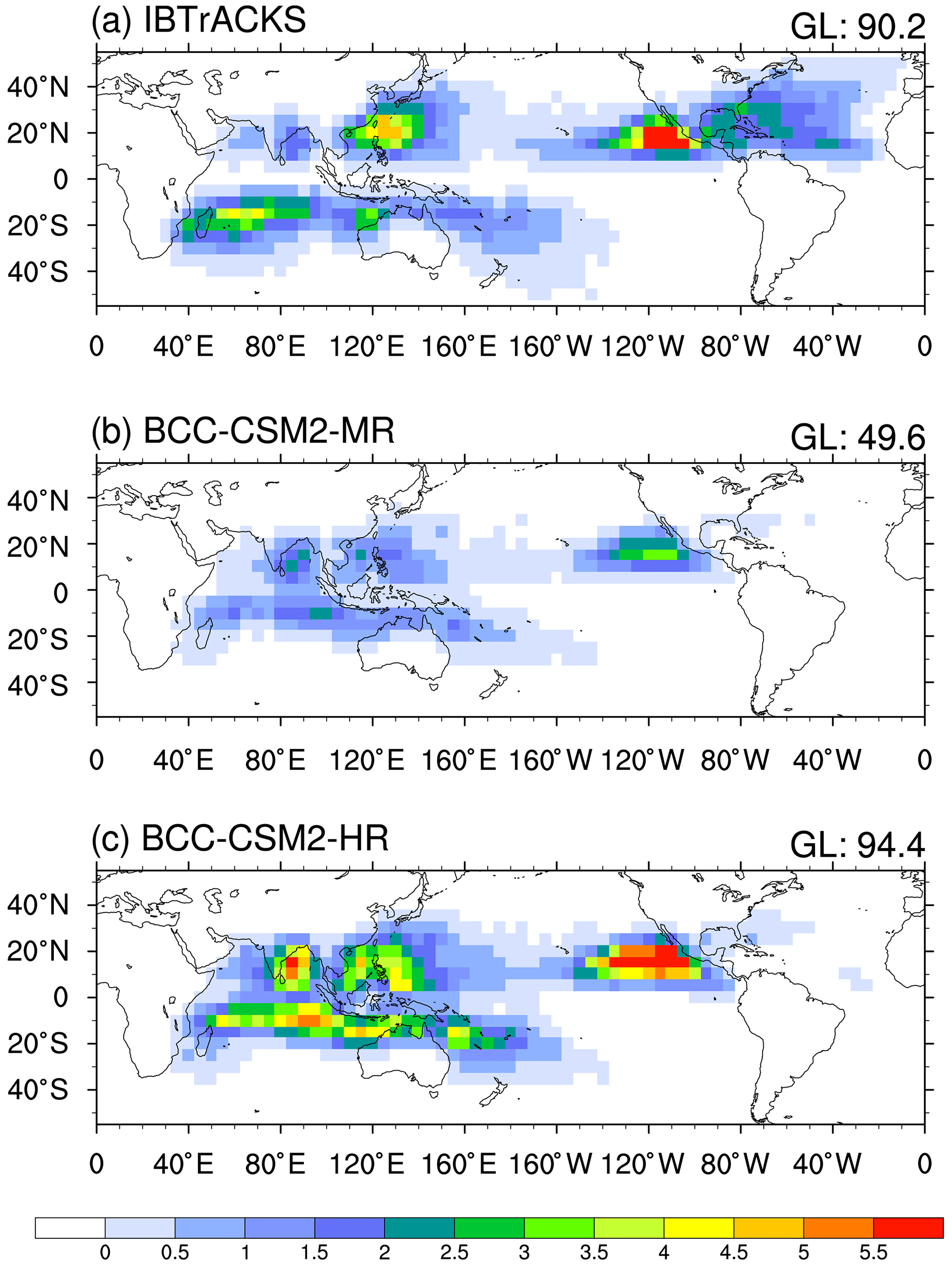
Figure 14 The global distribution of tropical cyclone (TC) densities (number per year) averaged for the period of 1995–2014 from (a) the IBTrACS_wmo observations, and the simulations of (b) BCC-CSM2-MR and (c) BCC-CSM2-HR. The value in the upper-right corner denotes the total number of global TCs on 5^∘ × 5^∘ grid box.

Figure 15 shows the maximum surface wind speed versus minimum sea level pressure for the tropical cyclones that are derived from the 1995–2014 IBTrACS observation (black dots and line) and simulations of BCC-CSM2-MR and BCC-CSM2-HR. Here, the maximum surface wind speed (minimum sea level pressure) of a given TC was defined as the instantaneous maximum (minimum) of the 6 h interval in IBTrACS and BCC-CSM2-HR, but the averaged value in BCC-CSM2-MR for wind speed at 10 m (sea level pressure). Instantaneous values of wind speed and sea level pressure were not recorded as output in BCC-CSM2-MR. Maximum wind speeds for TC lifetime in BCC-CSM2-MR are consistently weaker than BCC-CSM2-HR and IBTrACS, which is understandable given the coarser resolution. BCC-CSM2-MR cannot capture strong storms, and maximum wind speeds at 10 m only reach 30 m s⁻¹. BCC-CSM2-HR, as expected, can reproduce those strong TCs for which minimum pressure of TC lifetime may reach 960 hPa and maximum wind speed at 10 m may reach 50 m s⁻¹. The fitting line of maximum wind speeds with minimum centre pressures in BCC-CSM2-HR almost matches that from IBTrACS observation (Fig. 15). The BCC-CSM2-HR simulations demonstrate, just as previous studies have shown (e.g. Murakami et al., 2012; Sugi et al., 2017; Vecchi et al., 2019), that the maximum wind speed of TC simulated by a model with approximately 50 km resolution can reach up to 50–60 m s⁻¹.

Figure 15 Maximum surface wind speed (m s⁻¹) versus minimum sea level pressure (hPa) for tropical cyclones from 6-hourly data for 1995–2014 IBTrACS observation (black dots and fitting line), and simulations from BCC-CSM2-HR (red dots and fitting line) and BCC-CSM2-MR (blue dots and fitting line). Each dot denotes the maximum surface wind speed and its corresponding minimum sea level pressure for a tropical cyclone during its lifetime.

4.4.2 Madden–Julian Oscillation

MJO is the dominant mode of sub-seasonal variability in the tropical troposphere (Madden and Julian, 1971) and characterized by eastward propagation of deep convective structures along the Equator with an average phase speed of around 5 m s⁻¹ at the intraseasonal timescale of 20–100 d (Wheeler and Kiladis, 1999). MJO generally forms over the Indian Ocean, strengthens over the Pacific Ocean, and weakens due to interaction with South America and cooler eastern Pacific SSTs (Madden and Julian, 1971). Figure 16 gives the time-lag–longitude evolution of 10^∘ S–10^∘ N-averaged intraseasonal precipitation anomalies in panels (a)–(c) and time-lag–longitude evolution of 80–100^∘ E-averaged intraseasonal precipitation anomalies correlated against the precipitation over the equatorial eastern Indian Ocean in panels (d)–(f). Both versions of BCC-CSMs reasonably reproduce the eastward propagating feature of convection from the Indian Ocean across the Maritime Continent to the Pacific (Fig. 16b and c), as well as the apparent poleward propagations from the equatorial Indian Ocean into the Northern Hemisphere and the Southern Hemisphere (Fig. 16e and f). The signal of northward propagation is more evident in BCC-CSM2-HR than in BCC-CSM2-MR. The average phase speed of eastward propagation of deep convection in BCC-CSM2-HR is much closer to GPCP data, denoted by the dashed line in Fig. 16c. Figure 16b shows that the eastward propagation of deep convection in BCC-CSM2-MR is too fast, compared to GPCP data.

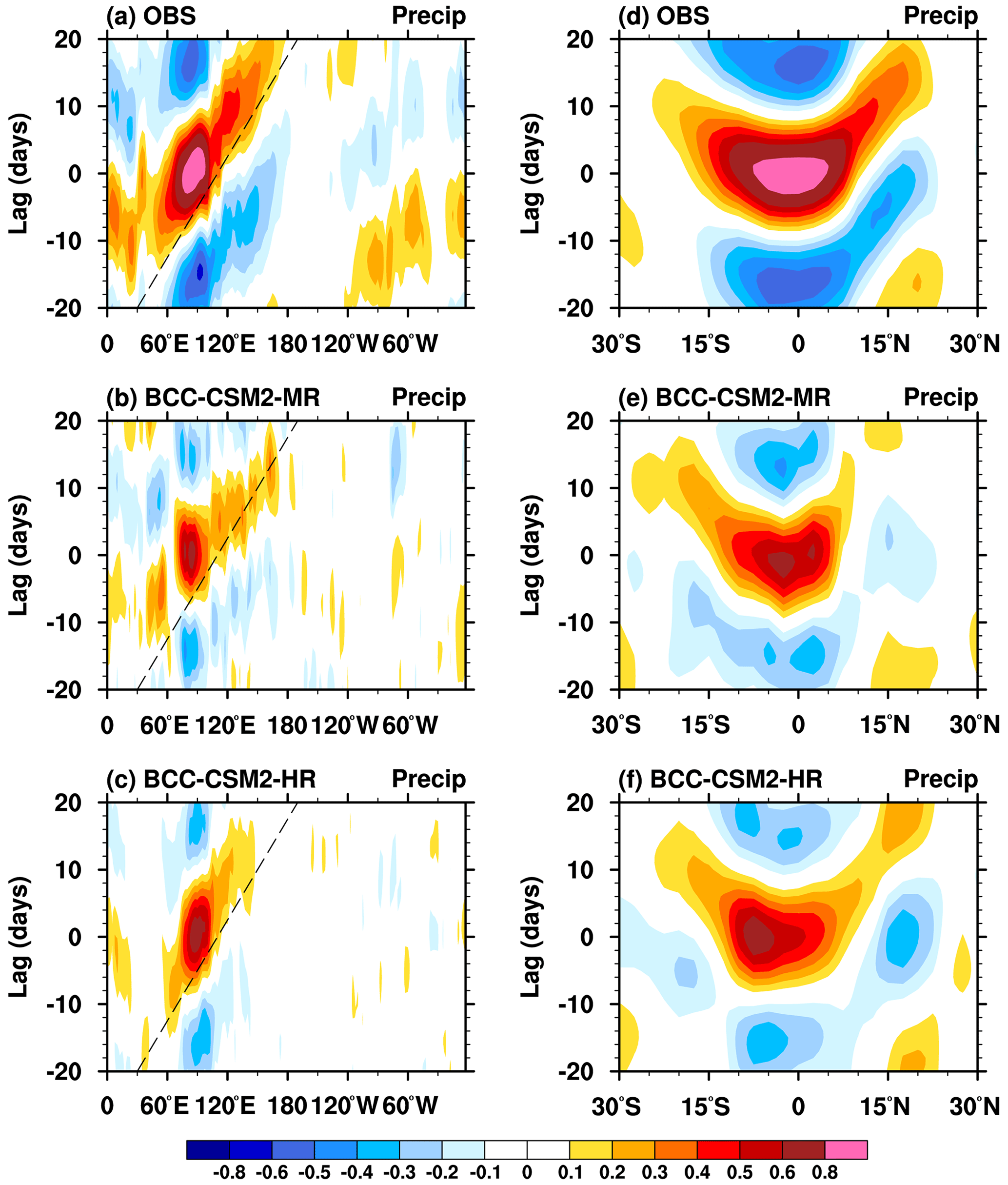
Figure 16 (a, b, c) Longitude–time evolution of lagged correlation coefficient for the 20–100 d band-pass-filtered precipitation anomaly (averaged over 10^∘ S–10^∘ N) against regionally averaged precipitation over the equatorial eastern Indian Ocean (80–100^∘ E, 10^∘ S–10^∘ N). (c, d, e) Same as the left panels, but for the latitude–time evolution of lagged correlation coefficients for filtered precipitation anomaly (averaged over 80–100^∘ E) against the regionally averaged precipitation over the equatorial eastern Indian Ocean. Dashed lines in each panel denote the 5 m s⁻¹ eastward propagation speed. The observations in (a) and (b) are derived from GPCP data and the simulations are from (c, d) BCC-CSM2-MR, and (e, f) BCC-CSM2-HR for the period from 1995 to 2014.

MJO activity can be generally featured by a life cycle of eight phases (Wheeler and Hendon, 2004). Intensity of outgoing longwave radiation (OLR) is often used for this purpose to represent the activity of convection. Figure 17 shows the MJO phase–latitude diagram of composited outgoing longwave radiation (OLR) and 850 hPa zonal wind anomalies averaged over 10^∘ S–10^∘ N. In observations, MJO convection initiated from Africa and the western Indian Ocean at phases 1–2, propagates eastward from the Indian Ocean across the Maritime Continent to the western Pacific at phases 3–6, and finally disappears in the western hemisphere at phases 7–8. BCC-CSM2-MR generally captures the evolution of convection with MJO phases but shows faster propagative speed and apparently underestimates the intensity compared to the observation. In contrast, BCC-CSM2-HR shows an obviously improved MJO phase transition and convection intensity.

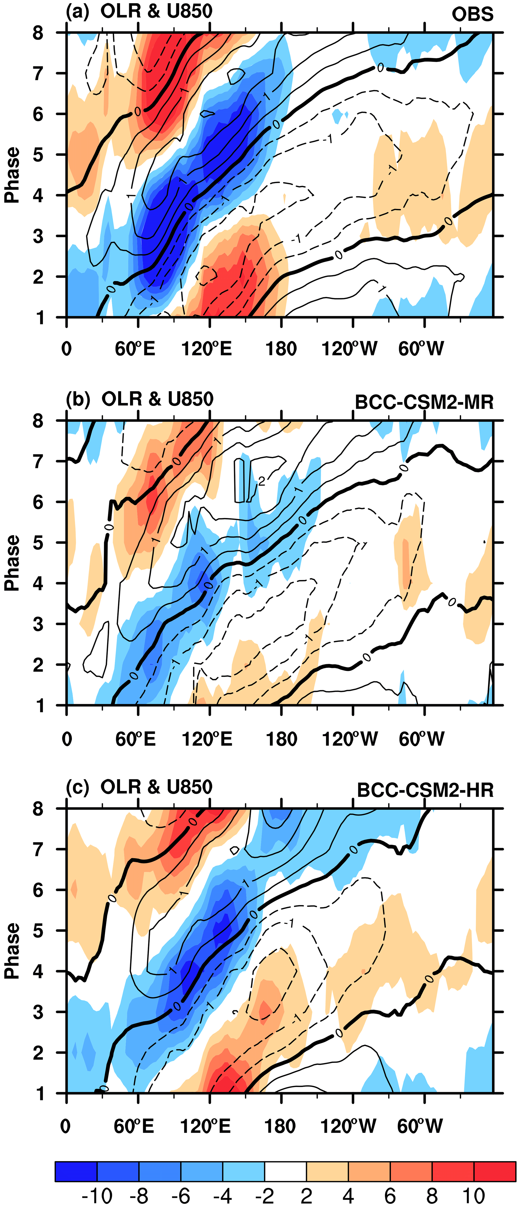
Figure 17 Hovmøller diagrams of MJO phase-composited OLR (shaded) and 850 hPa zonal wind anomalies (contour lines) averaged between 10^∘ S and 10^∘ N from (a) ERA5 wind and NOAA OLR reanalyses, (b) BCC-CSM2-MR, and (c) BCC-CSM2-HR simulations for the period from 1995 to 2014. The MJO phase is defined by the two principal components corresponding to leading multivariate EOFs of OLR, 850 and 200 hPa zonal wind anomalies as in Wheeler and Hendon (2004).

4.4.3 The stratospheric quasi-biennial oscillation

The alternative oscillation between westerly and easterly winds in the tropical stratosphere constitutes the characteristic feature of the quasi-biennial oscillation (QBO). A good simulation of QBO still remains a challenge nowadays for all state-of-the-art climate models. In a recent work, Kim et al. (2020) showed that only half (15 out of 30) of the CMIP6 models can internally generate QBO (BCC-CSM2-MR was in the good half). We should, however, recognize that there was huge progress in CMIP6, since in CMIP5 only five models (about 10 % of the total) were able to simulate a realistic QBO (Schenzinger et al., 2017).

To evaluate model performance in simulating the QBO, the time–height cross sections of the tropical zonal winds averaged from 5^∘ S to 5^∘ N for BCC-CSM2-MR and BCC-CSM2-HR are compared to the ERA5 reanalysis. As shown in Fig. 18, ERA5 shows alternative westerlies and easterlies in the lower stratosphere with a mean periodicity of about 28 months. The two BCC models are both able to generate a reasonable QBO, and the observed asymmetry with the easterlies being stronger than the westerlies is also well reproduced. The general performance of QBO in BCC-CSM2-MR was evaluated in Wu et al. (2019b). A detailed assessment of the underlying mechanism involving wave dynamics and the associated forcing to drive QBO is presented in Lu et al. (2020a). The simulated QBO has stronger amplitudes in BCC-CSM2-HR than in BCC-CSM2-MR. As the horizontal resolution and physics package are changed from BCC-CSM2-MR to BCC-CSM2-HR, the parameterized convective gravity wave forcing for QBO could be potentially enhanced in BCC-CSM2-HR. On the other hand, changes in the convective cumulus parameterization can also affect the simulation of the resolved convectively coupled equatorial waves (i.e. the Kelvin wave) driving the QBO and lead to stronger QBO amplitudes in BCC-CSM2-HR.

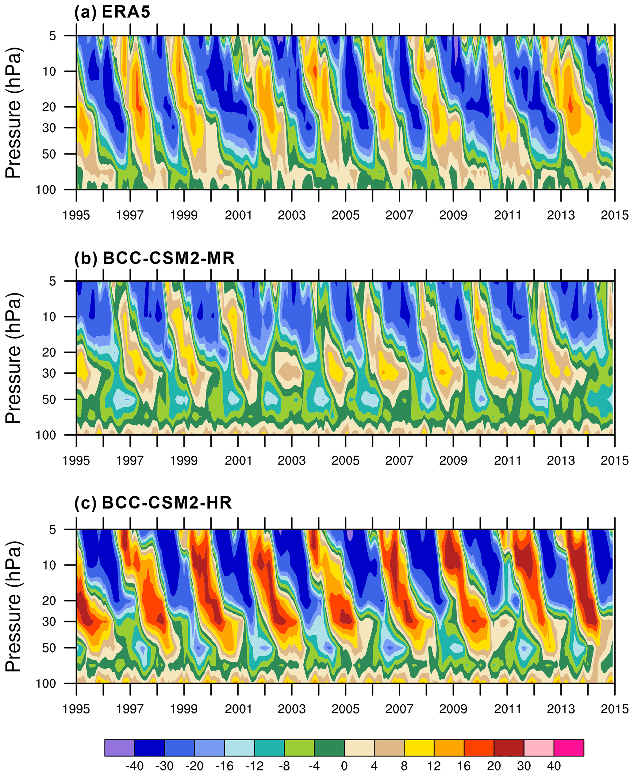
Figure 18 Tropical zonal winds (m s⁻¹) between 5^∘ S and 5^∘ N in the lower stratosphere for (a) ERA5 reanalysis, (b) BCC-CSM2-MR, and (c) BCC-CSM2-HR during the period from 1995 to 2014.

In the two BCC models, the downward propagation of QBO occurs in a regular manner but does not sufficiently penetrate to low altitudes below 50 hPa. The vertical resolution is similar below ∼ 10 hPa in both BCC-CSM2-MR and BCC-CSM2-HR (Fig. 1). A further downward propagation to lower altitudes can be expected by increasing the vertical resolution finer than 500 m to adequately resolve the wave-mean flow interaction in the upper troposphere and lower stratosphere (Geller et al., 2016; Garcia and Richter 2019).

4.4.4 Niño3.4 SST variability 

Figure 19 presents time series of the monthly Niño3.4 SST (5^∘ N–5^∘ S, 170–120^∘ W) anomalies from BCC-CSM2-MR and BCC-CSM2-HR, with reference to HadISST data from 1950 to 2014. The amplitude of interannual variation of the Niño3.4 index in BCC-CSM2-HR and BCC-CSM2-MR are both stronger than in HadISST. Those strong amplitudes may partly come from the slight warming trends in both models. The power spectrum analysis of the Niño3.4 index from the HadISST observations shows significant peaks at 4–6 and 2–3 years. The periodicity of the ENSO cycle in BCC-CSM2-MR is mainly at 2–3 years. It is prolonged to 3–6 years in BCC-CSM2-HR. As in Fig. 19h, the Niño3.4 SST variability from HadISST data reaches its maximum in the period from November to January. The phase locking (i.e. the preferred timing in the year for the peak of ENSO) simulated by BCC-CSM2-MR occurs in autumn. The simulated ENSO phase locking in BCC-CSM2-HR is partly improved, since ENSO events tend to reach their maximum toward winter.

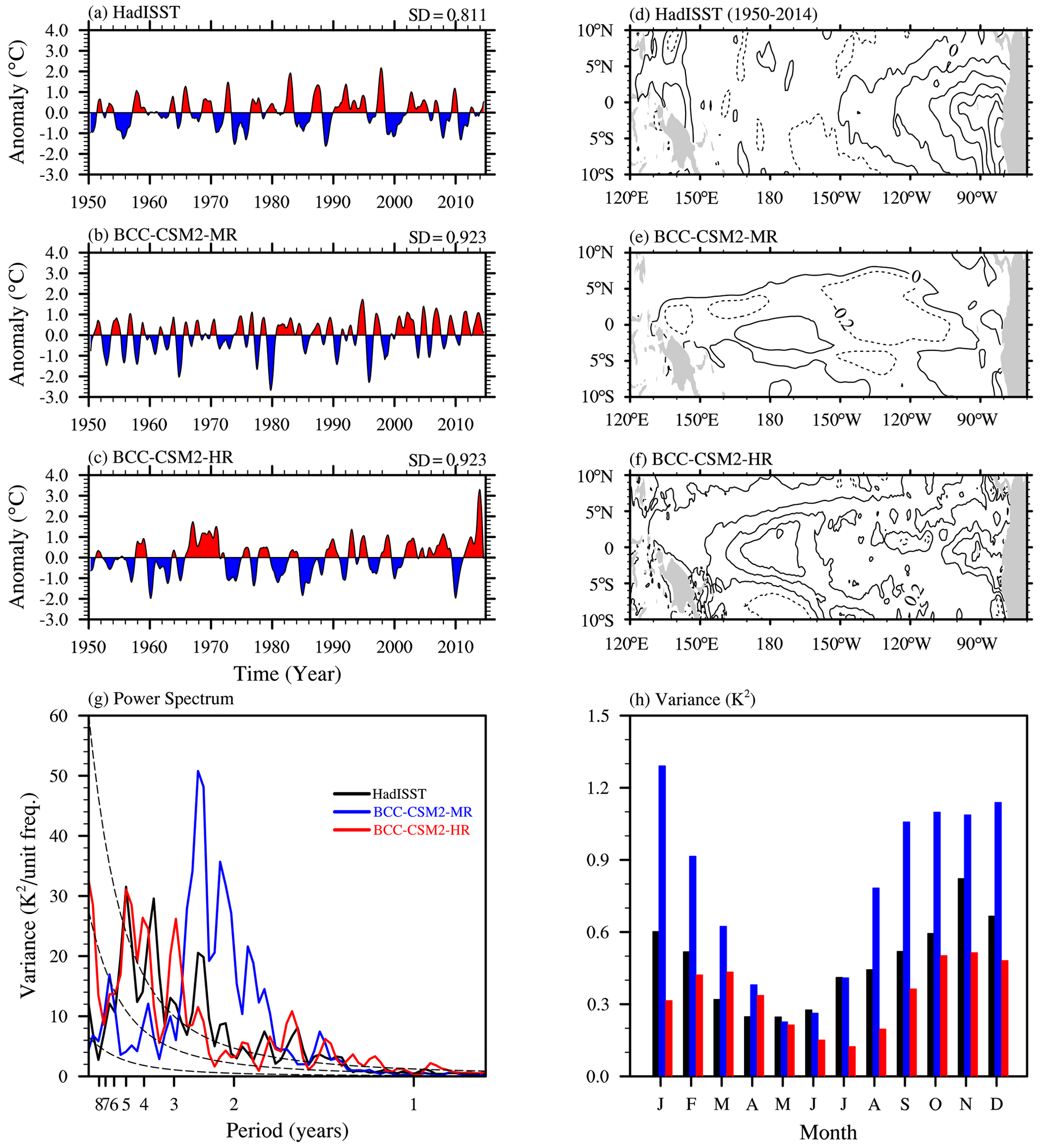
Figure 19 The time series of monthly Niño3.4 SST (5^∘ N–5^∘ S, 170–120^∘ W) anomalies and spatial distribution of their skewness for (a, d) HadISST observation, (b, e) BCC-CSM2-MR, and (c, f) BCC-CSM2-HR during the period 1950–2014. Panels (g) and (h) show their power spectrums and variances, respectively, and the black, blue, and red solid lines denote the results from HadISST, BCC-CSM2-MR, and BCC-CSM2-HR.

Recent studies of Hayashi et al. (2020) showed that the ability to simulate the asymmetry between warm (El Niño) and cold (La Niña) phases as recorded in observations is still very poor for most CMIP5 and CMIP6 models. This imperfection also exists in both BCC-CSM2-HR and BCC-CSM2-MR. The asymmetry in SST anomalies is often measured by the normalized third statistical moment, i.e. skewness (Burgers and Stephenson, 1999). Figure 19d–f show spatial maps of the skewness of monthly SST anomalies (SSTA) in the tropical Pacific that are calculated following the methodology in Burgers and Stephenson (1999). In the eastern Pacific, the ENSO signal from HadISST data is the strongest and the observed SSTA skewness is highly positive (Fig. 19d) due to the presence of extreme El Niño events and absence of extreme La Niña events. The skewness values of SSTA in both models (Fig. 19e and f) are underestimated in contrast to HadISST observation, and the area of positive skewness in the eastern tropical Pacific from BCC-CSM2-HR simulations is much closer to HadISST data.

Figure 20 presents the spatial patterns of correlation coefficients between the Niño3.4 index and the corresponding global SST anomalies from 1950 to 2014 for the HadISST observation and the two BCC models. Both BCC-CSM2-HR and BCC-CSM2-MR simulate a positive correlation structure over the equatorial region of the central and eastern Pacific, which is consistent with the analysis from HadISST despite an over-extension into the western Pacific. The HadISST data show clearly that the zone of positive correlation of SST with the Niño3.4 index in the equatorial eastern Pacific expands to the extra-tropics. Especially along the eastern border of the Pacific, the areas of high values of positive correlations in BCC-CSM2-HR are larger than BCC-CSM2-MR, and much closer to HadISST. Compared to BCC-CSM2-MR, BCC-CSM2-HR improves the simulation in the equatorial Indian Ocean and the eastern tropical Atlantic where there are also remarkable areas of positive correlation. We also note that areas of negative correlation of SST with the Niño3.4 index in the western equatorial Pacific extend to the South and North Pacific in HadISST, which is clearer in BCC-CSM2-HR than in BCC-CSM2-MR.

Figure 20 Correlation coefficients between SST and the Niño3.4 index from 1950 to 2014 for (a) HadISST data, (b) BCC-CSM2-MR, and (c) BCC-CSM2-HR. Contour intervals are 0.2. Values significant at the 99 % level using a Student's t test are stippled.

5 Conclusions and discussions

This paper was devoted to the presentation of the high-resolution version BCC-CSM2-HR and to the description of its climate simulation performance. We focused on its updates and differential characteristics from its predecessor, the medium-resolution version BCC-CSM2-MR. BCC-CSM2-HR is our model version participating in HighResMIP, while BCC-CSM2-MR is our basic model version participating in other CMIP6-endorsed MIPs (Wu et al., 2019b; Xin et al., 2019).

The atmosphere resolution is increased from T106L46 in BCC-CSM2-MR to T266L56 in BCC-CSM2-HR, and the ocean resolution from $\mathrm{1}{}^{\circ }\times \mathrm{1}{}^{\circ }$ to $\mathrm{1}/\mathrm{4}{}^{\circ }\times \mathrm{1}/\mathrm{4}{}^{\circ }$. A few novel developments were implemented in BCC-CSM2-HR for both the dynamical core and model physics in the atmospheric component: first, a spatially varying damping for the divergence field was used to improve the atmospheric temperature simulation in the stratosphere at polar areas – it helps to control high-frequency noise in the stratosphere and above; second, the deep cumulus convection scheme originally described in Wu (2012) was further ameliorated to allow detrained cloud water be transported to adjacent grids and downward to lower troposphere; third, we modified the relevant schemes for the boundary layer turbulence and shallow cumulus convection to improve the simulation of ITCZ precipitation; fourth, the UWMT scheme is used to improve the simulation of low-level clouds over eastern basins of subtropical oceans. The land model configuration in BCC-CSM2-HR is the same as in BCC-CSM2-MR. Major land surface biophysical and plant physiological processes of BCC-AVIM2 implemented in BCC-CSM2-MR and BCC-CSM2-HR were kept the same, and the only differences are in the sub-grid surface classification. The ocean component of BCC-CSM2-HR is upgraded from MOM4 in BCC-CSM2-MR to MOM5. The sea-ice component is also updated from SIS4 to SIS5.

For the sake of a rigorous comparison, historical simulations with fully coupled BCC-CSM2-MR and BCC-CSM2-HR are analysed over a 65-year period from 1950 to 2014. The long-term trends of 1950–2014 globally averaged annual-mean surface air temperature from both BCC-CSM2-MR and BCC-CSM2-HR are highly correlated to HadCRUT4 observation. The global warming in the latter half of the 20th century is well simulated, and the observed global warming hiatus or slowdown in the period from 1998 to 2013 is generally captured by both model versions.

We compared the 1995–2014 basic climate features in relation to atmospheric temperature, circulation, precipitation, surface temperature, and sea ice between the two simulations and we evaluated them against observation-based and reanalysis data. With contrast to the medium-resolution BCC-CSM2-MR, the high-resolution BCC-CSM2-HR has slightly improved energy equilibrium for the whole Earth system. The global mean TOA net energy balance is about 1.51 W m⁻² in BCC-CSM2-HR for the period from 1995 to 2014, showing an evident improvement compared to 2.12 W m⁻² in BCC-CSM2-MR. The longwave and net cloud radiative forcing are overall consistent with CERES-EBAF at most latitudes, but excessive cloud radiative forcing for shortwave radiation is found over the eastern tropical Pacific and tropical Atlantic in BCC-CSM2-HR. Temperature biases in the low- to mid-troposphere below 300 hPa in BCC-CSM2-HR are relatively small, within the range of −1 to 1 K. Both versions of BCC-CSMs have a cold air temperature bias that appears above 250 hPa in the subpolar and polar region, and a warm bias in the upper stratosphere at the mid-latitudes, which caused westerly wind biases in the upper troposphere and in the stratosphere. Although those prominent systematic biases in temperature and wind seem relatively insensitive to changes in atmospheric resolution, the ability to capture the winter-to-summer seasonal transition in the vertical structure of temperature and wind in the upper stratosphere is strengthened in BCC-CSM2-HR.

The two versions of BCC-CSM were both able to reproduce the observed global precipitation patterns, and there is a remarkable improvement in precipitation centres over the Pacific, Indian, and Atlantic oceans in the high-resolution model. The double-ITCZ biases in BCC-CSM2-MR are reduced in BCC-CSM2-HR, and excessive precipitation in the South Pacific Convergence Zone is also strongly reduced in BCC-CSM2-HR. The climatological SST in BCC-CSM2-HR, relative to the observation-based HadISST data, shows cold but reduced biases compared to BCC-CSM2-MR. Such SST cold biases are partly attributable to different ocean components, MOM4 in BCC-CSM2-MR and MOM5 in BCC-CSM2-HR. The seasonal cycles of amplitude and phase of sea ice in both hemispheres are generally well captured in BCC-CSM2-HR, but with a small excess all year round in the Northern Hemisphere, especially in the Atlantic.

We also conducted an assessment on a few important phenomena of the tropical climate, such as TC (tropical cyclone), MJO (Madden–Julian oscillation), QBO (quasi-biennial oscillation), and ENSO (El Niño–Southern Oscillation). The averaged total number of global TC in BCC-CSM2-HR is a bit larger than in IBTrACS observation. BCC-CSM2-HR can simulate main TC activities in the eastern North Pacific, Northern Indian, and in the Southern Hemisphere but misses the TC activities in the North Atlantic. BCC-CSM2-HR is able to capture a realistic MJO signal including the eastward-propagating behaviour of MJO and its phase speed. The QBO-related alternative westerlies and easterlies in the tropical lower stratosphere with a mean periodicity of about 28 months are well simulated. The weakness in downward propagation of the simulated QBO (insufficient penetration of the signal to low altitudes) in BCC-CSM2-MR is slightly improved in BCC-CSM2-HR. Main features of the ENSO cycle such as the periodicity and phase locking are captured by BCC-CSM2-HR although its main ENSO periodicity of 3–6 years is still shorter compared to HadISST observations.

Our work shows that enhancing resolution does not noticeably improve climate mean state, and deterioration is even possible. For example, the decrease in JJA precipitation over the warm pool in our high-resolution model is still an important issue which certainly deserves further investigations with multiple models and simulations. Actually, other studies also reported similar issues. Haarsma et al. (2020) shows that increasing resolution in the EC-Earth model deteriorated the wet bias over the western Pacific warm pool. Bacmeister et al. (2014) analysed the high-resolution climate simulations performed with the Community Atmosphere Model (CAM) and showed that dry bias over the same region with enhanced resolution. Over the western Pacific warm pool, the atmospheric circulation and precipitation undergoes not only the impact of tropical variations such as MJO and TC, but also strong regional air–sea coupling.

We finally should note that there exist some systematic biases in our high-resolution model, such as the excessive cloud radiative forcing for shortwave radiation over the eastern tropical Pacific, cold biases in the near-surface temperature over northern Europe and over the tropical Atlantic, and insufficient TC activities over the North Atlantic and the Caribbean Sea. These are all important issues motivating us to develop and implement more physically based parameterizations in our future work. For the lack of sufficient TC activities in the North Atlantic, it seems that this bias also exists in other models (e.g. Bell et al., 2013; Strachan et al., 2013; Small et al., 2014) and still remains a challenging issue for the climate modelling community. A recent study reported by Davis (2018) showed that models with horizontal grid spacing of $\mathrm{1}/\mathrm{4}$^∘ or coarser could not produce a realistic number of category 4 and 5 storms in the tropical Atlantic. The spatial resolution even in our current high-resolution model seems too coarse.