the Creative Commons Attribution 4.0 License.
the Creative Commons Attribution 4.0 License.
 | 07 May 2021
Assessment of numerical schemes for transient, finite-element ice flow models using ISSM v4.18
Thiago Dias dos Santos
Mathieu Morlighem
Hélène Seroussi
Time-dependent simulations of ice sheets require two equations to be solved: the mass transport equation, derived from the conservation of mass, and the stress balance equation, derived from the conservation of momentum. The mass transport equation controls the advection of ice from the interior of the ice sheet towards its periphery, thereby changing its geometry. Because it is based on an advection equation, a stabilization scheme needs to be employed when solved using the finite-element method. Several stabilization schemes exist in the finite-element method framework, but their respective accuracy and robustness have not yet been systematically assessed for glaciological applications. Here, we compare classical schemes used in the context of the finite-element method: (i) artificial diffusion, (ii) streamline upwinding, (iii) streamline upwind Petrov–Galerkin, (iv) discontinuous Galerkin, and (v) flux-corrected transport. We also look at the stress balance equation, which is responsible for computing the ice velocity that “advects” the ice downstream. To improve the velocity computation accuracy, the ice-sheet modeling community employs several sub-element parameterizations of physical processes at the grounding line, the point where the grounded ice starts to float onto the ocean. Here, we introduce a new sub-element parameterization for the driving stress, the force that drives the ice-sheet flow. We analyze the response of each stabilization scheme by running transient simulations forced by ice-shelf basal melt. The simulations are based on an idealized ice-sheet geometry for which there is no influence of bedrock topography. We also perform transient simulations of the Amundsen Sea Embayment, West Antarctica, where real bedrock and surface elevations are employed. In both idealized and real ice-sheet experiments, stabilization schemes based on artificial diffusion lead systematically to a bias towards more mass loss in comparison to the other schemes and therefore should be avoided or employed with a sufficiently high mesh resolution in the vicinity of the grounding line. We also run diagnostic simulations to assess the accuracy of the driving stress parameterization, which, in combination with an adequate parameterization for basal stress, provides improved numerical convergence in ice speed computations and more accurate results.
- Article
(9141 KB) - Full-text XML
-
Supplement
(8766 KB) - BibTeX
- EndNote


Numerical modeling is routinely used to understand the past and future behavior of the ice sheets in response to the evolution of the climate (e.g., Ritz et al., 2015; DeConto and Pollard, 2016; Aschwanden et al., 2019; Goelzer et al., 2020; Seroussi et al., 2020). As is always the case with numerical models, one needs to minimize biases, numerical artifacts, or poor numerical convergence due to the choice of numerical scheme. It is therefore critical for the numerical solution to converge to the “true solution” regardless of the numerical scheme employed, and that the model is not overly sensitive to the mesh resolution (e.g., Szabó and Babuška, 1991, p. 4). One of the governing equations in ice-sheet numerical modeling is the mass transport equation, an advection equation derived from the conservation of mass that prescribes the evolution of the ice-sheet geometry (e.g., Cuffey and Paterson, 2010, p. 333). Another governing equation is the stress balance equation, a set of equations that describes the ice velocity over the entire ice sheet. This velocity field is used to “advect” the ice mass over time. These governing equations are often solved using numerical methods such as the finite-element method (FEM), widely employed in the ice-sheet modeling community (e.g., Larour et al., 2012; Gagliardini et al., 2013; Gudmundsson, 2020). As with any numerical method, several schemes exist to solve these equations within FEM in order to achieve stability, accuracy, and low computational cost, the desired properties of any numerical method (see, for example, Szabó and Babuška, 1991, Chapter 1).
It is well known that the discretization of advection-dominated equations by the traditional finite-element method leads to numerical instabilities and spurious oscillations (e.g., John et al., 2018). The mass transport equation therefore needs to be stabilized when solved using FEM. The choice of an adequate stabilization scheme is crucial to simulate the main characteristics of ice-sheet dynamics without introducing numerical artifacts in the solution, such as oscillations, non-physical diffusion, or poor numerical convergence (see, e.g., John and Schmeyer, 2008). While some stabilization techniques may have good properties for some specific applications, they may not be appropriate for others.
The finite-element method's literature presents a large number of stabilization schemes, with different levels of complexity and accuracy (Codina, 1998; Franca et al., 2006; John and Schmeyer, 2008). The simplest schemes are based on adding an artificial diffusive-type term, turning the advection equation into an advection–diffusion equation (LeVeque, 1992, p. 118). This approach is equivalent to the upwind differencing employed in the finite-difference method (Kelly et al., 1980; Selmin, 1993). While this method leads to a more stable formulation, the downside is the reduced accuracy especially in regions where the solution is not smooth or presents steep gradients (Brooks and Hughes, 1982; Donea, 1984b). Other schemes are based on counterbalancing the terms in the finite-element formulation, such that the numerical diffusion vanishes (Brooks and Hughes, 1982). A popular method is the streamline upwind Petrov–Galerkin (SUPG), but the accuracy and stability of this scheme rely on the definition of the stabilization parameter, which is problem-dependent (Almeida and Silva, 1997; Codina, 2000; Knopp et al., 2002; Bochev et al., 2004; John and Schmeyer, 2008; Burman, 2010). Alternatively, a discontinuous Galerkin (DG) formulation, a finite-volume-inspired scheme, produces accurate results in advection-dominated flows (Cockburn, 1998, 1999). However, its implementation requires specific data structures to handle (computational) nodes and (geometric) vertices of the mesh (e.g., Calle et al., 2005; Devloo et al., 2007). Also, the increased number of degrees of freedom introduced by this method may reduce the computational performance. Most recently, finite-element-oriented flux-correction schemes have been proposed as a promising alternative (Kuzmin and Turek, 2002; Kuzmin et al., 2003). These schemes manipulate the discretized algebraic system in order to add anti-diffusive terms without compromising numerical stability. All the schemes described above have been applied to a number of physical problems (e.g., Reed and Hill, 1973; Jameson, 1995; John and Schmeyer, 2008; Ngo et al., 2015; Watanabe and Kolditz, 2015; Diddens, 2017; Hansen et al., 2019). However, the performance of these schemes has not been evaluated in a systematic way for ice-sheet simulations.
The stress balance is another critical component of transient models. For simplified stress balance equations, such as the shallow shelf approximation (MacAyeal, 1989) or Blatter–Pattyn's higher-order models (Blatter, 1995), the right-hand side is a function of the ice surface gradient (Cuffey and Paterson, 2010, p. 295). Usually, in finite-element-based ice-sheet models, gradients are assumed to be continuous within each element. This is a reasonable assumption for most of the ice-sheet domain, except at the grounding line, the point where ice detaches from the underlying bedrock and starts to float over the ocean. From a numerical simulation point of view, the grounding line represents a discontinuity of several physical processes (e.g., basal friction, basal melt), and the accuracy of its dynamics requires a fine mesh resolution (Durand et al., 2009; Pattyn et al., 2012, 2013; Cornford et al., 2013). Sub-element parameterizations of such physical processes are commonly employed to improve numerical convergence of the ice velocity computation (Seroussi et al., 2014a; Feldmann et al., 2014; Cornford et al., 2016; Seroussi and Morlighem, 2018). In most basal friction parameterizations, for instance, the grounding line is free to evolve within the elements. Generally, in such a situation, the models assume the ice thickness to be continuous at the grounding line1. This assumption implies that, for the grounded part of the element crossed by the grounding line, the ice surface is a function of both bedrock elevation and ice thickness, while, for the floating part, the ice surface is obtained by the hydrostatic floatation only, which only depends on the ice thickness. This makes the gradient of the ice surface and the resulting driving stress discontinuous within the elements containing the grounding line. While there exist comparison studies for basal friction and basal melt parameterizations (e.g., Seroussi et al., 2014a; Seroussi and Morlighem, 2018), little attention has been given to the sub-element parameterization of the driving stress in the context of the finite-element method. To the best of our knowledge, only studies based on finite-volume and finite-difference methods use driving stress parameterizations (Cornford et al., 2013; Feldmann et al., 2014).
In this context, the present paper aims to (i) assess the response of different stabilization schemes in transient simulations subject to ice-shelf basal melt and changes in basal friction, and (ii) develop and assess a sub-element parameterization for the driving stress. The numerical experiments are based on the Marine Ice Sheet Model Intercomparison Project for plan-view models (MISMIP3d) setup (Pattyn et al., 2013), a simple idealized ice-sheet geometry. Additional experiments are presented for the Amundsen Sea Embayment (ASE) of the West Antarctic Ice Sheet (WAIS), which includes the Pine Island and Thwaites glaciers. We use the Ice-sheet and Sea-level System Model (ISSM) to perform all the numerical experiments. In Sects. 2 and 3, we describe the technical details of the stabilization schemes and driving stress parameterization, respectively, and in Sect. 4 we present the numerical setup of experiments used to test them. The results are shown in Sect. 5, followed by discussions in Sect. 6 and final remarks in Sect. 7.
2.1 Mass transport equation
The evolution of the ice thickness is described by an advection equation with source terms on the right-hand side:
where is the depth-averaged ice velocity in the horizontal plane, the surface mass balance (positive for accumulation), and the basal melt (positive for ablation). The velocity field is a function of the ice geometry and therefore of the ice thickness H. Note that both surface mass balance and basal melt may depend on the surface elevation and ice-shelf depth, respectively. All these dependencies make Eq. (1) a non-linear advection equation. For the sake of simplicity, we keep as a constant in all transient simulations. The description of is given in Sect. 4.1 (see Eq. 41).
The weak formulation of Eq. (1) is
where ℋ=ℋ(Ω) is a space of admissible functions for the model domain Ω, and ψ is called a test or weight function. We seek a solution H∈ℋ such that the weak form (Eq. 2) is satisfied. In the traditional finite-element method, both H and ψ belong to the same set of functions ℋ. It is known that in this approach Eq. (2) generates potentially large, spurious oscillations if not properly stabilized or if the mesh size is not excessively small (see, for example, Brooks and Hughes, 1982).
The weak form (Eq. 2) (and its alternative stabilized forms) requires approximating functions in ℋ with non-trivial first-order derivatives. In this sense, we employ subspace ℋ1⊂ℋ whose functions (and their first derivatives) are square integrable. For discretization purposes, we use P1 Lagrange functions and Delaunay-based triangulation.
2.2 Artificial diffusion and streamline upwinding
In general, stabilization schemes may be seen as a consistent way of adding terms to Eq. (1) (or Eq. 2) in order to transform it into a more stable formulation. In the artificial diffusion (ArtDiff; MacAyeal, 1997, p. 172) and streamline upwinding (Streamline; Hughes and Brooks, 1979; Kelly et al., 1980) schemes, the resulting mass transport equation is
where 𝓓 is a second-order tensor, known as the diffusive tensor. In the artificial diffusion scheme, the tensor is defined as (MacAyeal, 1997, p. 172)
where h is the characteristic size of the element, and vx and vy are the horizontal components of the (depth-averaged) ice velocity. In the streamline upwinding method, the tensor is defined in such a way that the artificial diffusion is added only along streamlines and not in cross flows. In this sense, the tensor 𝓓 is defined as (Hughes and Brooks, 1979; Kelly et al., 1980; Brooks and Hughes, 1982)
where is the Euclidean norm. The resulting weak formulation of Eq. (3), after integrating the diffusive term by parts, is
Both schemes are interpreted as an upwind-equivalent scheme employed in the finite-difference method (Kelly et al., 1980; Selmin, 1993), sharing therefore similar characteristics such as a first-order accuracy and large numerical dissipation (de Vahl Davis and Mallinson, 1976; Gresho and Lee, 1979). However, the resulting formulation is very stable, which made them popular in glaciology (e.g., MacAyeal, 1997, p. 172). Artificial diffusion was the default scheme employed in ISSM. The low accuracy of such schemes leads to the development of alternative methods with higher accuracy, such as the streamline upwind Petrov–Galerkin.
2.3 Streamline upwind Petrov–Galerkin
In the SUPG scheme (Brooks and Hughes, 1982), the diffusive or upwind term is not added directly into Eq. (1). Instead, the upwind effect is achieved by adding the upwinding term into the test function ψ (Christie et al., 1976; Heinrich et al., 1977). This procedure, where the solution and test functions belong to different spaces, is commonly called Petrov–Galerkin method (see, e.g., Griffiths and Lorenz, 1978; Brooks and Hughes, 1982). The modified test functions are generally defined as (Brooks and Hughes, 1982)
where τ is a stabilization coefficient, defined below. Using the modified test functions , the resulting weak formulation of Eq. (1) is written as
The most common definition of the stabilization term τ is given by (Franca et al., 2006)
with
where Pe is the Péclet number of element e, and κ is known as the diffusion coefficient. The diffusion coefficient κ is not explicitly defined in Eq. (1). For fast ice streams where the flow is dominated by basal sliding rather than internal deformation2, an alternative is to assume the asymptotic limit of the term within parentheses in Eq. (9) when κ and consequently Pe go to infinity. With this assumption, the stabilization coefficient is approximated by
An alternative to defining τ is to replace the Péclet number by the Courant–Friedrichs–Lewy (CFL) number Ce in Eq. (9) (Gudmundsson, 2020, p. 19, 20), i.e.,
with
where Δt is the simulation time step. The motivation behind this approach is the equivalence between the SUPG and Taylor–Galerkin methods in transient problems (see, e.g., Donea, 1984a; Donea et al., 1984; Codina, 1998; Blank et al., 1999; Akin and Tezduyar, 2004; Kuzmin, 2010, p. 73). For Ce≪1, which is basically true in ice-sheet simulations3, the term within parentheses in Eq. (12) is approximately (Gudmundsson, 2020, p. 20). Therefore, for low CFL numbers, we can approximate Eq. (12) by
In ISSM, we implement τ as given by Eq. (11), i.e., τ=τ1. This definition is also employed in Elmer/Ice, a popular FEM-based ice-sheet model (Gagliardini et al., 2013). However, for some simulations performed here, we use the approximation given by Eq. (14) (τ=τ2), as implemented in Úa (Gudmundsson, 2020), another popular ice-sheet model.
2.4 Discontinuous Galerkin
Strictly speaking, DG is not exactly a stabilization scheme in the sense of adding upwinding terms to Eq. (1) or to the space of test functions ψ. It is a variant of the traditional continuous Galerkin method, in which the functions approximating the solution are discontinuous across elements' edges. This adds the advantage of local conservation with typical FEM characteristics such as the ease of dealing with non-structured meshes, complex domains, and boundary conditions, and hp adaptivity (Cockburn, 1998; Kuzmin, 2010, p. 84). With appropriate definition of the numerical inter-element fluxes, the resulting formulation is known to be stable in advection-dominated problems (e.g., Brezzi et al., 2004). It was originally developed for the neutron transport simulation (Reed and Hill, 1973), and since then DG has been applied to other fields, including elliptic-type equations (e.g., Babuška et al., 1999; Brezzi et al., 2000; Arnold et al., 2002). A more complete history and an overview of the vast application fields of DG can be found in Cockburn (1998, 2003).
In DG, the weak formulation is written in an element-wise fashion, and the advection operator is integrated by parts such that Eq. (2) is rewritten as
where Ωe∈Ω is the domain of element e, Se is the boundary of Ωe, ℋ is built on the element's domain (i.e., ℋ=ℋ(Ωe)), and n is a unit vector pointing outward along the boundary Se. The stabilized version of Eq. (15) comes from the definition of the numerical flux () in the second integral on the left-hand side. In ISSM, an upwinding numerical flux is employed such that Eq. (15) is rewritten as (Brezzi et al., 2004)
where is the upwinding numerical flux.
As seen in Sect. 2.6, the time-derivative discretization of Eq. (16) in ISSM relies on a backward Euler scheme, which differs from the popular Runge–Kutta discontinuous Galerkin (RKDG; Cockburn and Shu, 1991; Cockburn, 1998, 2003), an explicit time projection scheme that is known for its stability (as long as ) and allows full parallelization since the resulting mass matrix is block diagonal. The DG implementation in ISSM was conceived to be an alternative to other stabilization schemes without enforcing large changes in an existing code. Therefore, we do not expect to achieve the same benefits as RKDG (and similar schemes) in our simulations. The Elmer/Ice model (Gagliardini et al., 2013) adopts a time discretization similar to the implementation of ISSM.
2.5 Flux-corrected transport
The flux-corrected transport (FCT) scheme operates in the resulting algebraic system of the traditional Galerkin discretization (i.e., Eq. 2) instead of modifying its weak form or the approximation/trial spaces. The scheme was developed to solve the continuity equation for compressible fluids in a finite-difference framework (Boris and Book, 1973), and it was extended to FEM by Löhner et al. (1987) and most recently by Kuzmin and Turek (2002) and Kuzmin et al. (2003). The latter is also named as FEM-FCT in the literature. The FEM-FCT scheme seems to be stable even in the presence of steep gradients and discontinuities (e.g., John and Schmeyer, 2008). For simplicity, we refer to the FEM-FCT scheme as FCT. This scheme can be described as a hybrid method combining a higher-order (but potentially oscillatory) scheme and a lower-order diffusive (not oscillatory) scheme. In regions where the solution is smooth, the higher-order scheme is applied, while the lower-order scheme is applied where necessary (e.g., steep gradient regions). However, this scheme adds just enough flux into the “low-order region” from the high-order (a.k.a. anti-diffusive) region to maintain its accuracy without inducing oscillations.
The scheme modifies the discrete form of Eq. (2) by employing a generic finite-difference scheme for the time derivative, i.e.,
where Δt is the time step, MC is the mass matrix4, K is the advection matrix, and F is the forcing vector. The superscripts n+1 and n indicate the next and current steps, and the fractional weight θ stands for the backward Euler scheme if θ=1 and for Crank–Nicolson if . As explained in Sect. 2.6, the load vector F as well as the velocity field in K are defined in step n. To simplify the notation, we drop the superscripts of these variables in this section.
The first step consists of turning Eq. (17) into a stable, low-order algebraic system. This is achieved by replacing the consistent mass matrix MC by a lumped mass matrix ML and the advection matrix K by a matrix L:
where N is the total number of degrees of freedom. The matrix L is defined as
where D={dij} represents an artificial diffusion with elements defined as (Kuzmin and Turek, 2002)
where kij are the elements of matrix K (={kij}). By construction, the matrix L does not contain any positive off-diagonal elements. The resulting stable, low-order system of equations is
Compared to the original system (Eq. 17), the modified system (Eq. 21) creates large numerical diffusion that prevents spurious oscillations. By doing so, however, it also reduces the accuracy of solution Hn+1.
In order to improve the accuracy of the solution while still preventing spurious oscillations, the second step of the scheme consists in adding an anti-diffusive term to the right-hand side of Eq. (21):
where F* is a vector whose elements are defined as
In Eq. (23), are weights to be defined appropriately (see below and Appendix A), and R={rij} is based on the residual vector R between Eqs. (21) and (17):
The residual vector R can be decomposed as (see, e.g., Kuzmin, 2009)
where rij represents the raw anti-diffusive flux from node j into node i. Using Eqs. (18) and (20), rij can be written as (John and Schmeyer, 2008)
Note that rij depends on the solution Hn+1. Roughly speaking, there are two approaches to proceed with Eq. (26): (i) a non-linear algorithm and (ii) a linear algorithm. Here, we describe the latter (Kuzmin, 2009), which is currently implemented in ISSM. Further details of both approaches can be found in John and Schmeyer (2008) or in Kuzmin (2009).
In the linear FCT algorithm, the solution Hn+1 in Eq. (26) is replaced by the solution HL obtained in the low-order system (Eq. 21), i.e.,
In ISSM, the Crank–Nicolson scheme (i.e., ) is used in Eq. (27), and the raw anti-diffusive flux (Eq. 26) is replaced by an alternative form (Kuzmin, 2009):
where is an approximation of the time derivative . This approximation is computed using Richardson's iteration:
with . The convergence of Eq. (29) usually takes one to five iterations (Kuzmin, 2009).
Once the anti-diffusive flux is obtained by Eq. (28) using Eqs. (27) and (29), the last step is to compute the solution Hn+1. In this linearized FCT version, the solution Hn+1 is explicitly obtained by solving (Kuzmin, 2009)
where F* is obtained by Eq. (23) with rij computed by Eq. (28). The weights αij are obtained using the so-called Zalesak algorithm (Zalesak, 1979). Appendix A presents the algorithm as implemented in ISSM.
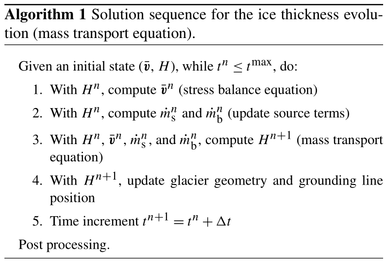
2.6 Time discretization of the mass transport equation
We employ a semi-implicit finite-difference time-stepping scheme to solve the temporal evolution of the ice thickness. This scheme involves a backward Euler method5 for the time derivative in Eq. (1), but the other variables (velocity, surface mass balance, and basal melting) are based on the previous time step. To illustrate this scheme, we apply this time-derivative discretization in Eq. (6), as follows:
where Δt is the time step, and superscripts n and n+1 indicate the
current and next simulation steps,
respectively. Algorithm 1 presents the
solution sequence employed for the mass transport computation.
The position of the grounding line in non-full Stokes models is generally tracked with a level set condition based on a floatation criterion (Seroussi et al., 2014a). This level set can be located anywhere in an element, so it does not necessarily coincide with elements' edges:
where H is the ice thickness, ρ and ρw are ice and ocean densities, respectively, and r is the bedrock elevation (negative if below sea level). The ice is grounded if φ>0; otherwise, it is floating. The grounding line is implicitly defined where φ=0. In the element e containing the grounding line, the ice surface, s, is recovered as follows:
The second condition in Eq. (33) guarantees the continuity of the ice surface at the grounding line. However, its gradient is discontinuous within the element: in the grounded part (i.e., φ>0), the surface gradient is a function of both thickness and bedrock elevation, whereas in the floating part (φ<0), it is proportional to the thickness gradient only. The driving stress is therefore also discontinuous in elements partially floating and partially grounded, and we propose to use a sub-element driving stress parameterization to account for this discontinuity. A similar approach to subgrid cells was proposed (Cornford et al., 2013; Feldmann et al., 2014) based on finite-volume or finite-difference methods by applying one-sided differences to compute surface gradients on each side of the grounding line.
The driving stress parameterization is based on recovering the ice surface, and consequently its gradient, on the element e containing the grounding line. We divide the element domain Ωe in two subdomains: and that are the grounded and floating parts of the element, respectively (i.e., and ). We then perform the numerical integration of the driving stress on these two subdomains, i.e.,
where Fe is the element load vector, Ae is a matrix representing the rest of components of the driving stress and element basis functions6, and ∇s is evaluated according to the recovered ice surface (Eq. 33). For comparison purposes, we named the proposed driving stress parameterization SED2 (sub-element driving stress 2), since the approach here is similar to the basal friction parameterization SEP2 developed by Seroussi et al. (2014a). The non-parameterized case, i.e., when the ice surface is evaluated on the elements' vertices and then linearly interpolated elsewhere within the elements, regardless of the grounding line position, is referred to as no driving stress parameterization (NSED). Mathematically, the ice surface in the NSED scheme is defined as over Ωe, and the resulting driving stress is proportional to ∇H.
4.1 MISMIP3d – numerical setup
In this section, we describe the idealized geometry experiments used to evaluate the stabilization schemes and the proposed driving stress parameterization. For the latter, we employ different parameterization schemes for basal friction. The list of all the schemes tested is summarized in Table 1.
(Seroussi et al., 2014a)(Seroussi et al., 2014a)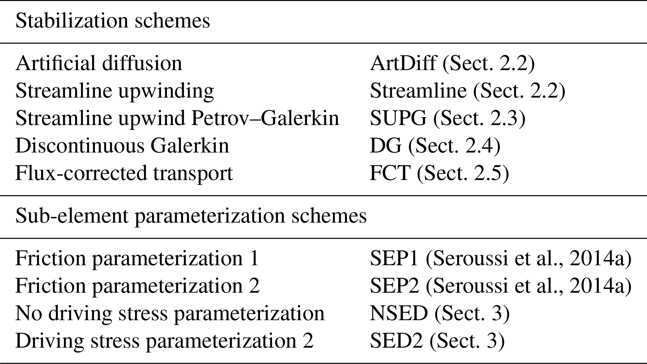
The numerical experiments are based on the MISMIP3d setup (Pattyn et al., 2013). The ice-sheet flows along the x axis in an 800×50 km2 rectangular domain entirely filled with ice. For the ice divide, x=0, we set vx=0. A free-slip condition is applied to the lateral boundaries of the domain, i.e., vy=0 for y=0 and y=50 km. The calving front is fixed in time and located at x=800 km, where we apply a Neumann boundary condition based on ocean water pressure. We employ a Weertman-type friction law given by
where τb is the basal friction, C is the friction coefficient, vb is the basal velocity, and m is the sliding law exponent. The bed elevation is defined as
where r(x,y) is the bedrock elevation (in meters; negative if below sea level), and x∈[0 800] is the x coordinate in kilometers. All experiments start from the same initial geometry, defined by the following ice thickness profile:
where H is the ice thickness, is the accumulation rate, xgl is the grounding line position (x axis), n is the Glen law exponent, Hgl and vgl are the ice thickness and the ice velocity (x direction) at the grounding line, respectively, defined as
and 𝒜 is defined by
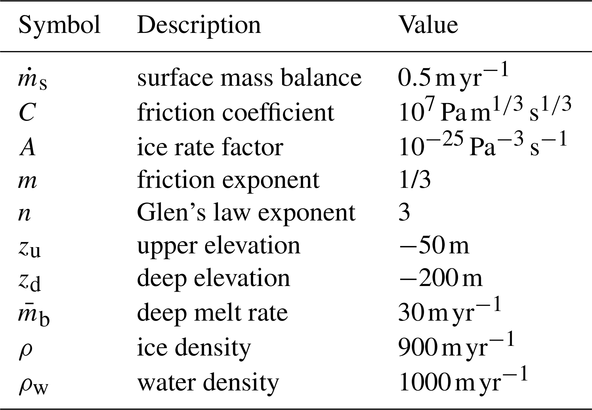
where A is the Glen law rate factor. The parameters used in all experiments are summarized in Table 2. In Eq. (37), the thickness expression for x<xgl is the steady-state profile of a 1-D ice sheet considering uniform accumulation rate and negligible longitudinal stresses (Schoof, 2007a). The x≥xgl case is the steady-state profile of an unconfined 1-D ice shelf under a uniform accumulation rate. Note that the initial thickness profile defined by Eq. (37) is a function of the grounding line position, xgl.
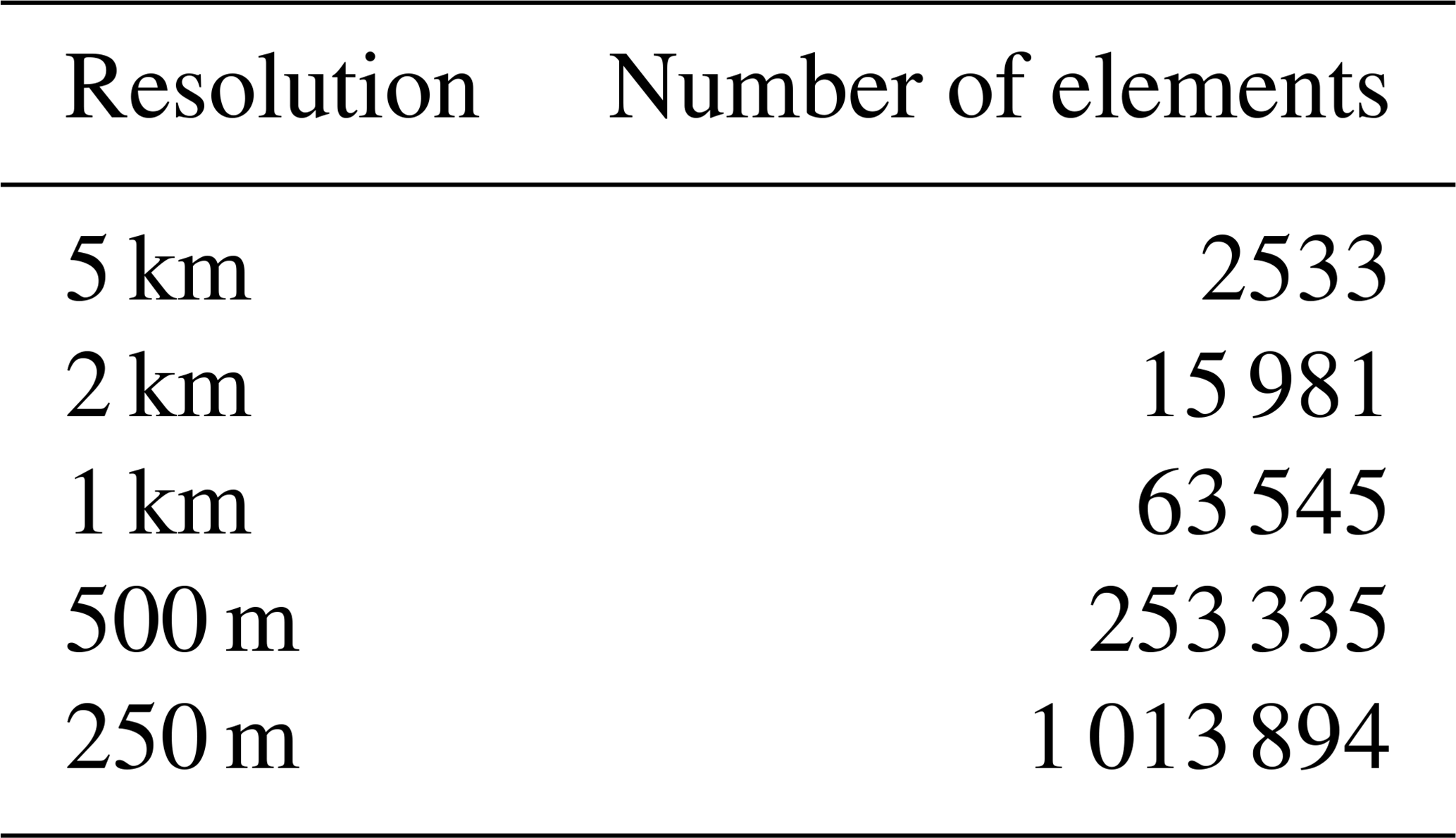
We define the initial grounding line position to be close to its steady-state position. According to boundary layer (Schoof, 2007a) and numerical convergence analyses employing SSA (Seroussi et al., 2014a), the grounding line should be located at x≃600 km. We therefore set xgl=600 km. Note that this steady-state grounding line position only applies to SSA models; other stress balance models (full Stokes, Blatter–Pattyn, L1L2, etc.) produce steady-state positions upstream of 600 km (Pattyn et al., 2013). The ice thickness as defined by Eq. (37) is not an exact steady-state profile but represents a slightly perturbed profile used to initialize all the experiments. The numerical models rely on unstructured triangular meshes (see some examples in Appendix B), and the mesh resolutions (and respective number of elements) chosen for the numerical convergence experiments are shown in Table 3. The analytical thickness (Eq. 37) is interpolated onto each vertex of the mesh, and the floatation criterion is applied to generate both surface and base profiles of the ice sheet. To enforce the same initial position of the grounding line (xgl) in the models, we employ a friction level set defined according to a distance-based function:
where φgr is the initial friction level set (positive if ice is grounded, and therefore friction is applied). The level set is evaluated at all elements' vertices.
The numerical experiments are divided in two sets of analyses: (i) diagnostic analysis and (ii) prognostic analysis. The diagnostic analysis consists of solving the stress balance equations under different sets of sub-element parameterization schemes (driving stress and basal friction; Table 1), with different mesh resolutions (Table 3). Here, we compare the ice speeds calculated by each set of sub-element parameterization schemes and mesh resolutions. We employ the two-dimensional SSA (MacAyeal, 1989) to compute the velocity field. The SSA equations are solved using Picard iterations and each linear system is solved using an iterative linear solver (conjugate gradient). The ice-sheet geometry is given by Eq. (37), with grounding line position defined by Eq. (40). The aim of the prognostic analysis is to solve the mass transport equation and compare the transient response using different stabilization schemes (Table 1). The transient simulations start from the same initial condition (Eq. 37) and grounding line position (Eq. 40) and run forward in time for 100 years under the same accumulation rate (; Table 2) under three different scenarios of external forcings: (i) no external forcing, (ii) basal melt under the ice shelf, and (iii) changes in basal friction. The first experiment (no external forcing) aims to analyze the models' adjustments under no external perturbation. In the second experiment, basal melt is applied at the base of the ice shelf in order to thin it, generating a large change in ice thickness close to the grounding line. Here, the basal melt is applied on (a) only fully floating elements and (b) fully and partially floating elements. It is important to note that applying melt on partly floating elements is not suitable for realistic marine ice-sheet simulations (see discussion in Seroussi and Morlighem, 2018), and we only assess the implications of using different stabilization schemes. In (a), no grounding line retreat is expected, since no buttressing effect is present in the initial condition (unconfined ice shelf). In (b), the grounding line is expected to retreat because part of the melt rate is applied on the first grounded vertices (Seroussi and Morlighem, 2018). The basal melt is defined below (see Eq. 41). The last experiment (friction perturbation) is based on the MISMIP3d perturbation phase, as a non-symmetric change in the basal friction coefficient is introduced. The goal of this experiment is not to assess grounding line reversibility, as proposed in the original MISMIP3d benchmark, but instead to assess the general migration of the grounding line (and resulting mass loss) for each stabilization scheme and different mesh resolution.
The basal melt applied in the second set of experiments is defined as follows (Seroussi and Morlighem, 2018):
where is the depth-dependent basal melting in m yr−1 (positive if melting), zb, in meters, is the vertical coordinate of the ice-shelf base (negative if below sea level), is the maximum melt rate for vertical coordinates equal to or lower than zd. We use m yr−1, m, and m, unless otherwise specified.
In all prognostic experiments, the grounding line is free to migrate, and its position over the simulation time is updated according to a hydrostatic floatation criterion, following Eq. (32): ice is floating (grounded) if the thickness, H, is lower (higher) than the floatation height, . The grounding line position is defined where H=Hf.
Table 2Constants and parameters used along the numerical experiments.
4.2 Amundsen Sea Embayment – numerical setup
In order to quantify the performance of the stabilization schemes with real ice-sheet geometries and numerical setups, we run transient simulations (prognostic analyses) of the ASE, which includes the fastest glaciers of WAIS. The glaciers in the ASE are subject to high ocean-induced melt rates and are prone to the marine ice-sheet instability (MISI), a positive feedback of grounding line retreat and increased ice discharge sustained by a retrograde bedrock slope (Weertman, 1974; Schoof, 2007b; Gudmundsson et al., 2012). Ice-shelf buttressing is present for most glaciers in the ASE, which helps stabilize the grounding line on retrograde slopes, reducing the possibility of MISI (Dupont and Alley, 2005; Goldberg et al., 2009; Docquier et al., 2014; Gudmundsson et al., 2019; Martin et al., 2019). Therefore, ice-shelf thinning plays an important role in the dynamics of this sector, and it is important to assess the impact of different stabilization schemes on the response of ASE due to ocean-induced melt and resulting sea-level-rise contribution.
Our ASE domain includes Pine Island, Thwaites, and neighboring glaciers (Haynes, Pope, Smith, and Kohler glaciers). We use BedMachine Antarctica v1 (Morlighem et al., 2020) to build the digital elevation model and interferometric synthetic aperture radar (InSAR)-derived surface velocities (Mouginot et al., 2019a) to infer basal friction coefficient and ice rheology using control algorithms (Morlighem et al., 2010, 2013). We generate the mesh based on an interpolation error estimate of the observed ice velocity and on the distance to the grounding line: a mesh resolution equal to 1 km is employed in the vicinity of the grounding lines, while coarser resolution (up to 16 km) is employed for the rest of the grounded ice. The mesh contains 261 375 elements and 131 087 vertices. Note that this is a typical numerical setup employed in many of ice-sheet studies (e.g., Favier et al., 2014; Joughin et al., 2014; Seroussi et al., 2014b; Cornford et al., 2015). Details of the model setup and initialization are described in Barnes et al. (2020).
For this setup, we perform only transient simulations with different stabilization schemes. All simulations start from the same initial condition and are forced by a constant surface mass balance obtained from the regional climate model (RACMO v2.3, Van Wessem et al., 2014) and the parameterized basal melt defined by Eq. (41). Here, the parameters in Eq. (41) are based on ice–ocean simulations (Seroussi et al., 2017; Nakayama et al., 2019): zu=0 and m. We run two basal melt scenarios based on different values of . For the first scenario, we set m yr−1 and, for the second one, m yr−1. Melt is applied only on fully floating elements. We chose the combination SEP1 + NSED as a set of parameterization schemes for basal friction and driving stress, respectively. The densities of ice and ocean are set to 917 and 1027 kg m−3, respectively. We run forward in time for 50 years with a fixed time step equal to one-eighth of a year. Like the other experiments performed here, the ice flow is computed by the SSA equations (MacAyeal, 1989).
5.1 MISMIP3d – diagnostic analysis
To compare the ice speed from different sets of sub-element parameterizations, we compute the speed from a reference model. The reference model is based on a triangular structured conforming mesh with resolution of 50 m. This structured conforming mesh is constructed in such a way that the elements' edges (around the grounding line) match perfectly the grounding line position (xgl=600 km; see Sect. 4.1; see also examples of structured meshes in Appendix B), and therefore no error related to driving stress and basal friction modeling is introduced in the stress balance computation in this reference model. We compare the speeds using two norms, the L2 norm and L∞ norm, defined as follows:
where is the absolute value of the ice speed, h and r refer to the mesh resolution and reference model, respectively. To evaluate the norms, the results from all models are interpolated onto a finer regular grid (25 m resolution), and the speed differences () are calculated on each vertex i of that grid. For the error convergence comparison, we also run models with structured meshes (conforming to xgl=600 km) considering the mesh resolutions shown in Table 3 (see examples in Appendix B). We refer to the speeds obtained by these conforming-mesh-based models as the reference speeds.

Figure 1Ice speeds obtained by the diagnostic analysis along a flow line (y=25 km) and around the grounding line (x=600 km, dashed line) for different mesh resolutions: 5000, 2000, 1000, and 500 m. All sets of sub-element parameterizations are shown: SEP1 + NSED, SEP2 + NSED, SEP1 + SED2, and SEP2 + SED2. The speed from the 50 m resolution structured conforming mesh (reference model) is also shown (reference, dotted line).
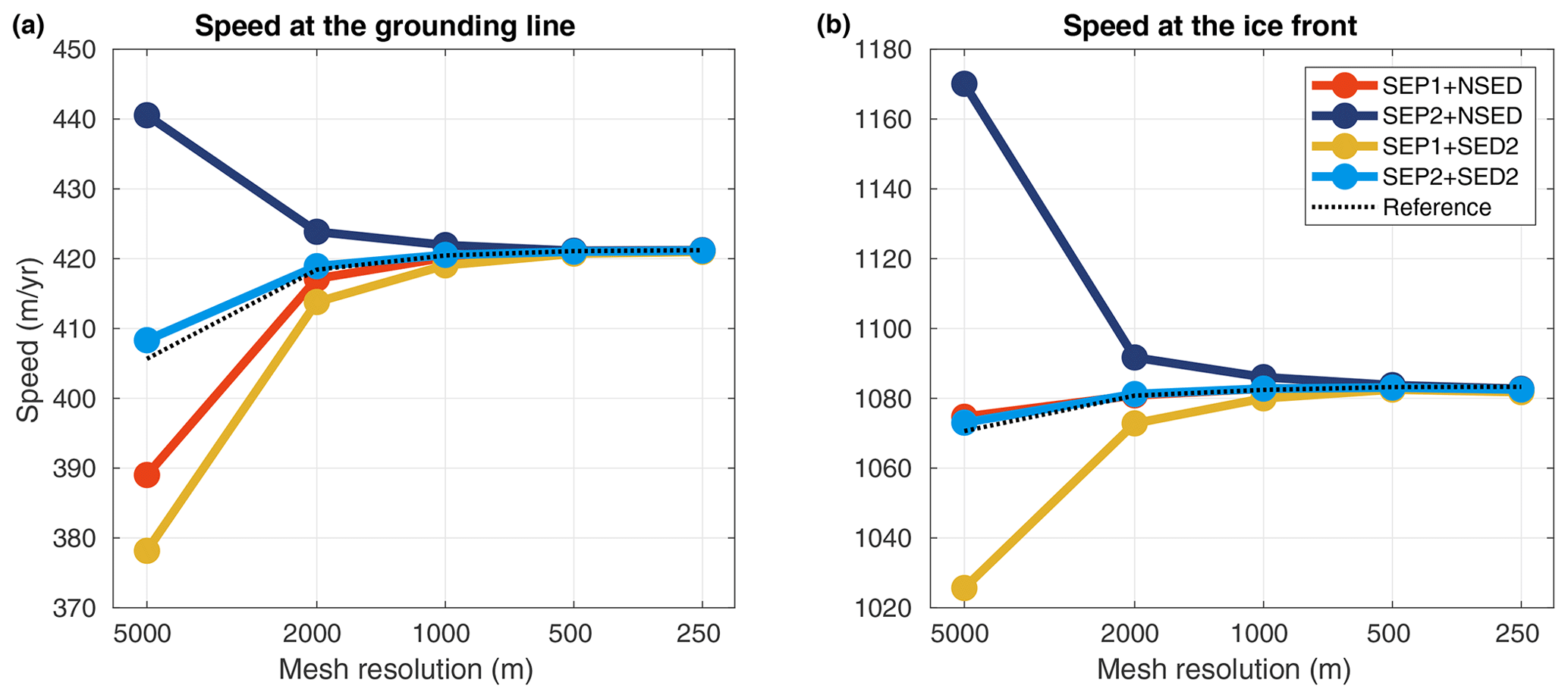
Figure 2Convergence of the ice speed at the grounding line (x=600 km, a) and at the ice front (x=800 km, b) obtained in the diagnostic analysis. All sets of sub-element parameterizations are shown: SEP1 + NSED, SEP2 + NSED, SEP1 + SED2, and SEP2 + SED2. Reference speeds from structured conforming-mesh-based models are also displayed (reference, dotted line).
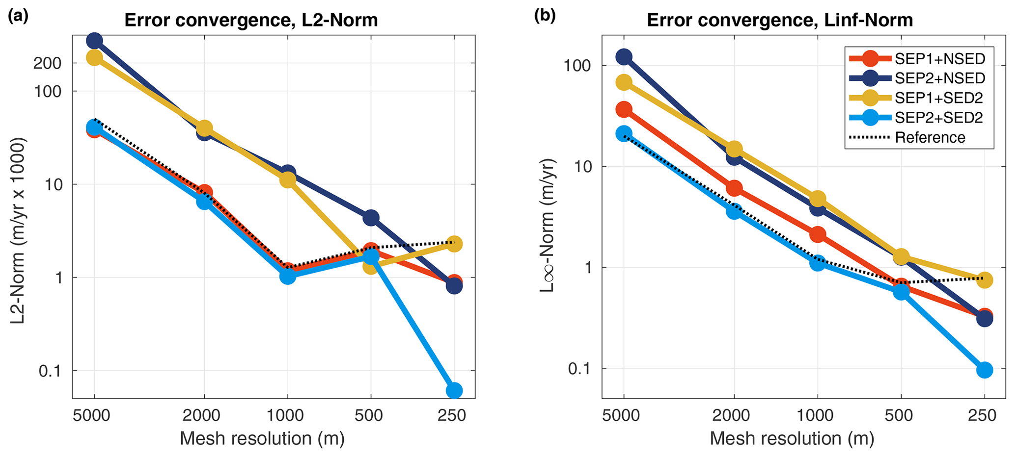
Figure 3Error convergence of the ice speed for the diagnostic analysis in L2 norm (a) and L∞ norm (b). All sets of sub-element parameterizations are shown: SEP1 + NSED, SEP2 + NSED, SEP1 + SED2, and SEP2 + SED2. The error convergence from structured conforming-mesh-based models is also shown (reference, dotted line).
Upstream of the grounding line, all sets of parameterizations “approach” the reference speed () for mesh resolutions finer than or equal to 1 km (Fig. 1). In the downstream part (floating ice), a 500 m mesh resolution or finer is required for all models to reach speeds at the grounding line and ice front similar to the reference model (Figs. 1 and 2). Overall, the errors in speed from models employing SEP1 + NSED and SEP2 + SED2 are closer to the ones obtained from structured conforming meshes (dotted line in Fig. 3). In other words, the convergence of sets SEP1 + NSED and SEP2 + SED2 is similar to the convergence of conforming-mesh-based models. The other combinations, SEP1 + SED2 and SEP2 + NSED, present relatively higher error levels in both norms (Fig. 3) for mesh resolutions coarser than 500 m.
5.2 MISMIP3d – prognostic analysis
We compare the transient results using the volume above floatation changes (ΔVAF) generated by each model and mesh resolution. The changes in VAF over time, t, are calculated as follows:
where h refers to mesh resolution and t0 is the initial time of the transient simulations. For some simulations, we also compare the grounding line positions at the end of the experiments. Based on the diagnostic analysis (Sect. 5.1), we employ the following sets of parameterizations in all transient simulations: SEP1 + NSED and SEP2 + SED2. We also compute the relative error in ΔVAFh obtained at the end of the experiments for a mesh resolution h, defined as
where 2h indicates the next coarser mesh resolution. We use similar quantities to compute the relative error in grounding line position at the end of the experiments, replacing ΔVAF by the grounding line position, GLpos, in Eq. (45).
5.2.1 No external forcing experiment
Since the initial ice-sheet profile (Eq. 37) is not exactly in steady state, some changes in VAF are expected to occur along the transient simulation due to grounding line adjustments (Fig. 4). In this control experiment, for mesh resolutions equal to or finer than 2 km, all stabilization schemes produce similar evolution of ΔVAF for both sets of parameterizations (Fig. 5). At the end of the experiment (t=100 years), all models produce a VAF loss equal to 116±4 Gt (Fig. 6). As shown in Fig. 6, the stabilization schemes generate different convergence curves of relative errors (except for streamline upwinding and artificial diffusion), but all show a decrease in error as the resolution increases, as expected. For a mesh resolution equal to 250 m, the relative errors for all stabilization schemes and sub-element parameterizations are below 5 % (Fig. 6).

Figure 4No external forcing experiment: ice surface and ice base at the end of the experiment (t=100 years) for different stabilization schemes (see legend). Two sets of parameterizations are employed: SEP1 + NSED (a) and SEP2 + SED2 (b). The dotted black line is the initial ice-sheet geometry, defined by Eq. (37). Here, the mesh resolution is equal to 500 m.
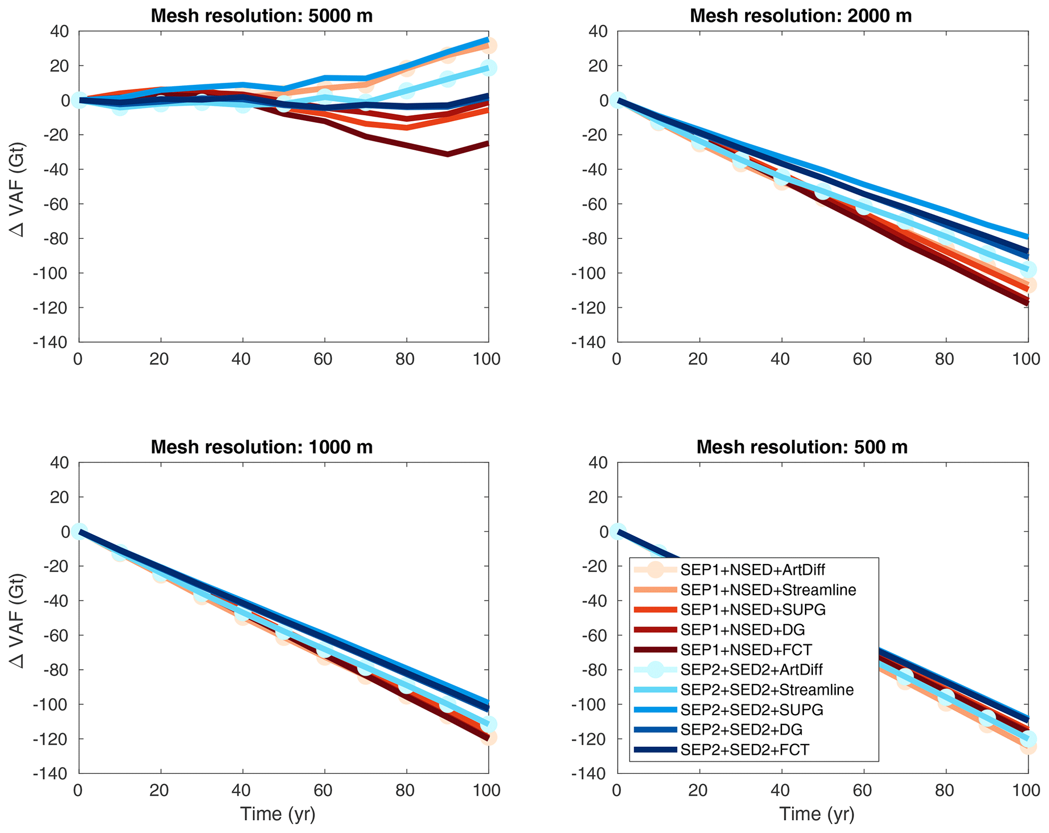
Figure 5No external forcing experiment: evolution of volume above floatation change (ΔVAF) for different mesh resolutions and stabilization schemes (see legend). Two sets of parameterizations are employed: SEP1 + NSED and SEP2 + SED2.
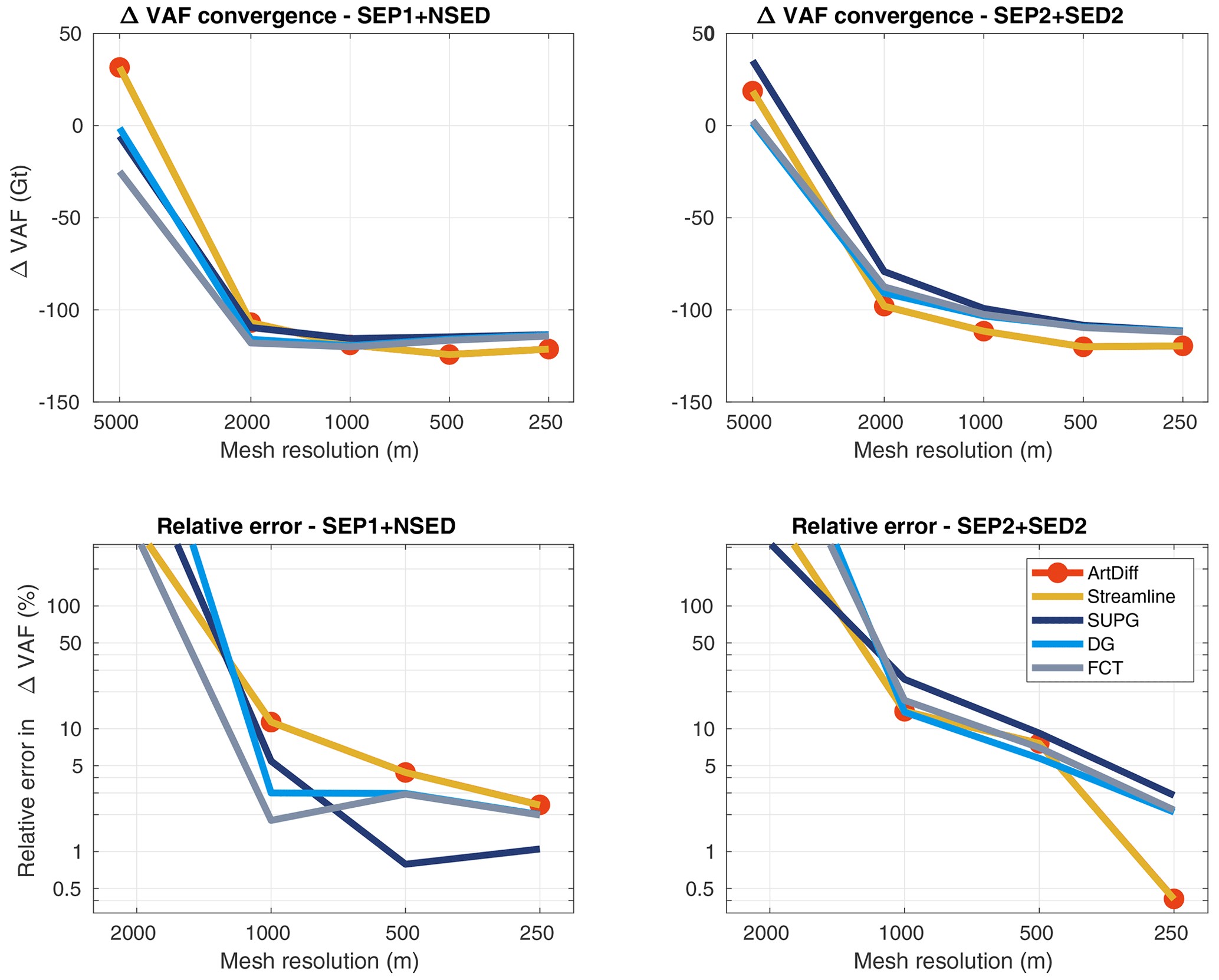
Figure 6No external forcing experiment: convergence of ΔVAF at the end of the experiment (t=100 years) for different stabilization schemes (see legend). Two sets of parameterizations are employed: SEP1 + NSED (left panels) and SEP2 + SED2 (right panels). The relative errors are computed using Eq. (45).
5.2.2 Basal melt experiment
In the setup where basal melt is applied only to fully floating elements (i.e., no melt on partly floating elements), models using artificial diffusion and streamline upwinding schemes produce almost 4 times the VAF losses observed in the control experiment (Fig. 7). At the end of the experiment, t=100 years, and for a mesh resolution equal to 500 m, the expected ΔVAF is Gt (see Sect. 5.2.1). A comparable amount of mass loss is obtained with models employing SUPG and discontinuous Galerkin. However, using artificial diffusion and streamline upwinding, the resulting ΔVAF is Gt, while with FCT, the ΔVAF reaches Gt (Fig. 8). The grounding line positions at the end of this basal melt experiment are expected to be close to the ones obtained with the control experiment (no external forcing). This is virtually achieved by models running with SUPG and discontinuous Galerkin, as illustrated on the left panel of Fig. 9. The grounding lines obtained from models employing artificial diffusion and streamline upwinding and even FCT have retreated further inland, resulting in an overestimated mass loss in comparison to SUPG and discontinuous Galerkin (Fig. 9). Both sets of sub-element parameterizations (SEP1 + NSED and SEP2 + SED2) lead to similar ΔVAF “convergence” for all stabilization schemes, although the convergence errors differ among them (Fig. 8). Only SUPG shows a decrease in relative error with mesh resolution, reaching error levels smaller than 10 % for a 250 m mesh resolution. Note that, in Fig. 8, artificial diffusion and streamline upwinding present relatively smaller errors in comparison to the others schemes (mainly DG and FCT), but the errors produced by these schemes do not decrease with mesh resolution and seem to be far from convergence, even for a mesh resolution of 250 m.
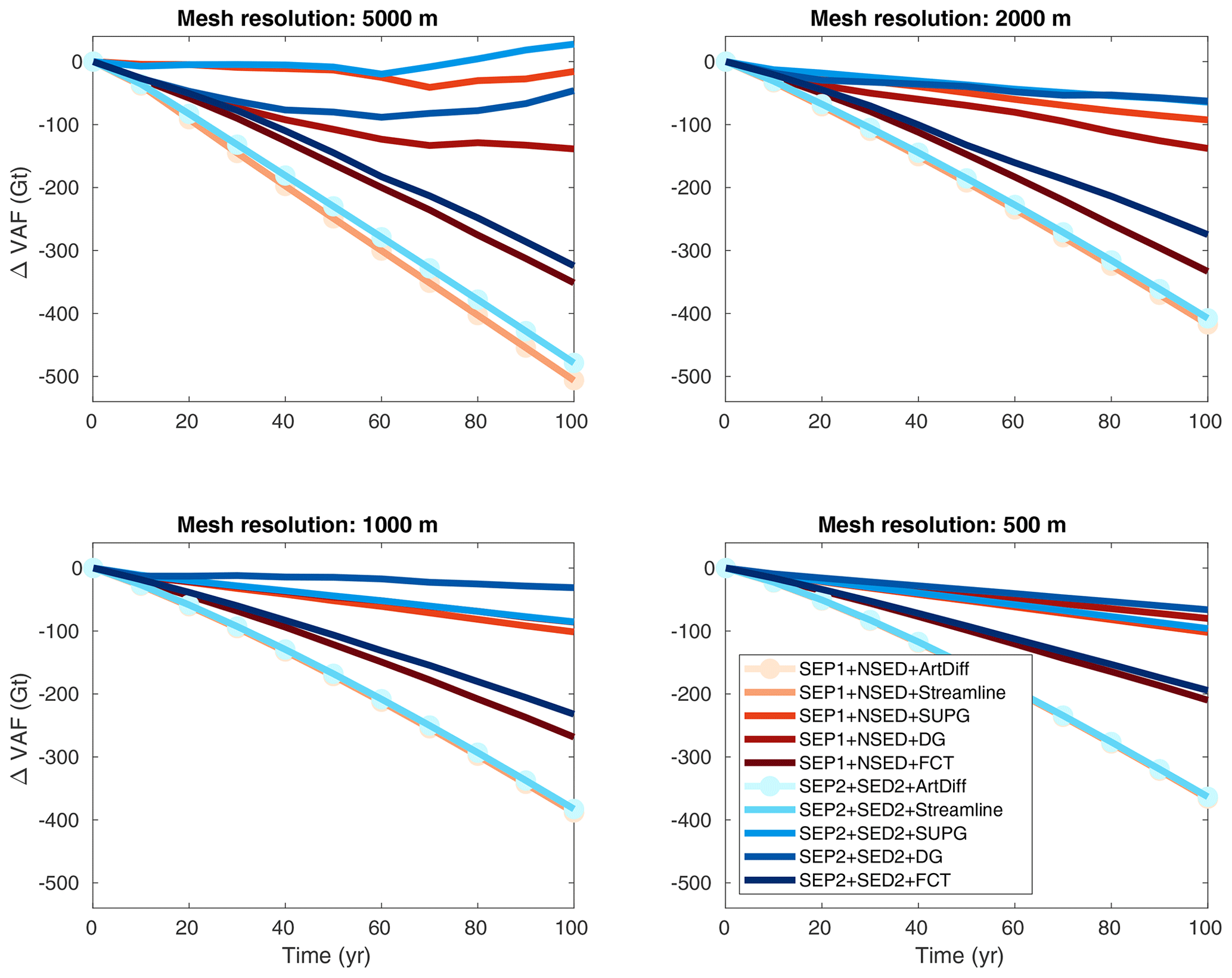
Figure 7Basal melt experiment (no melt on partly floating elements): evolution of ΔVAF for different mesh resolutions and stabilization schemes (see legend). Two sets of sub-element parameterizations are employed: SEP1 + NSED and SEP2 + SED2.
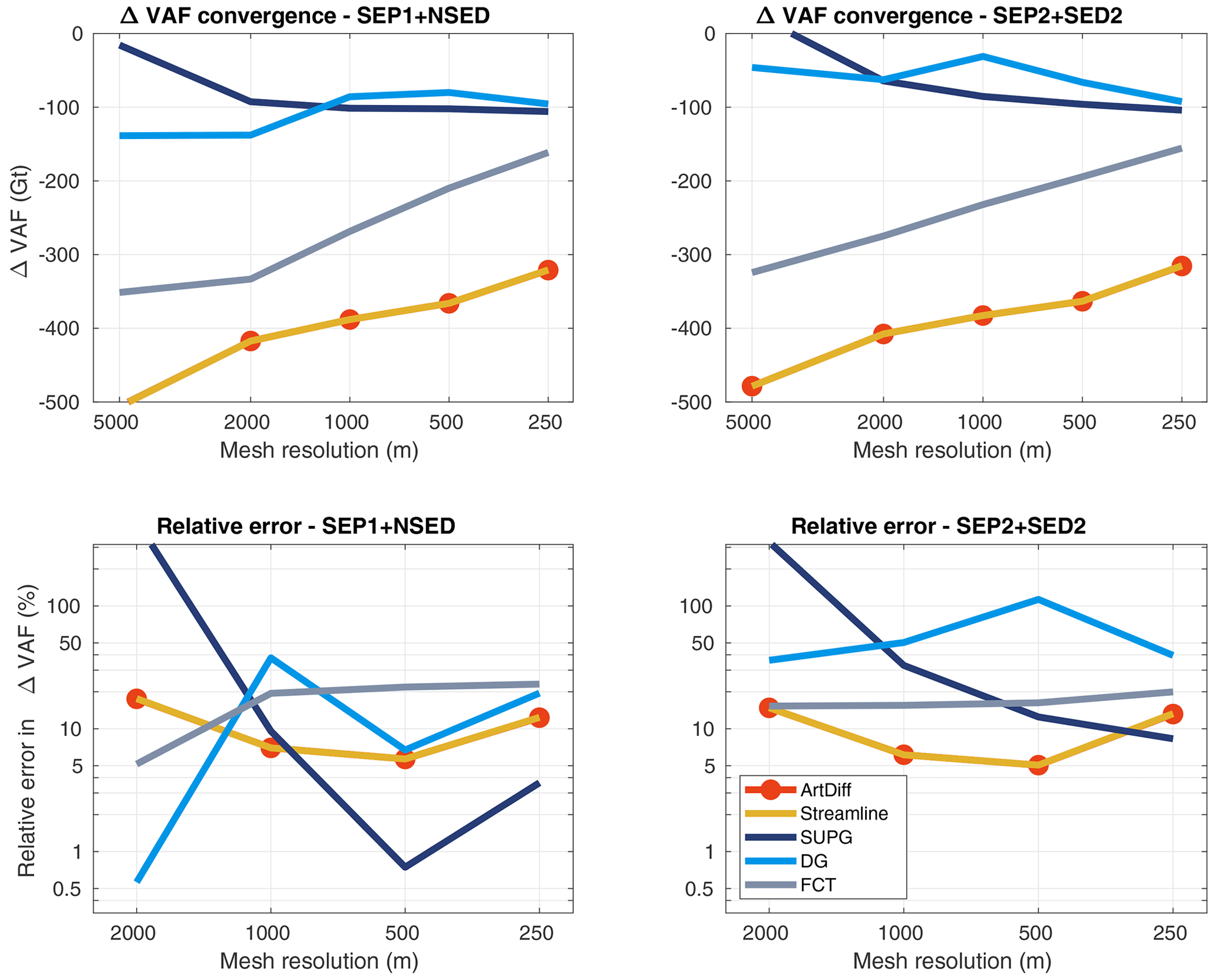
Figure 8Basal melt experiment (no melt on partly floating elements): convergence of ΔVAF at the end of the experiment (t=100 years) for different stabilization schemes (see legend). Two sets of sub-element parameterizations are employed: SEP1 + NSED (left panels) and SEP2 + SED2 (right panels). The relative errors are computed using Eq. (45).
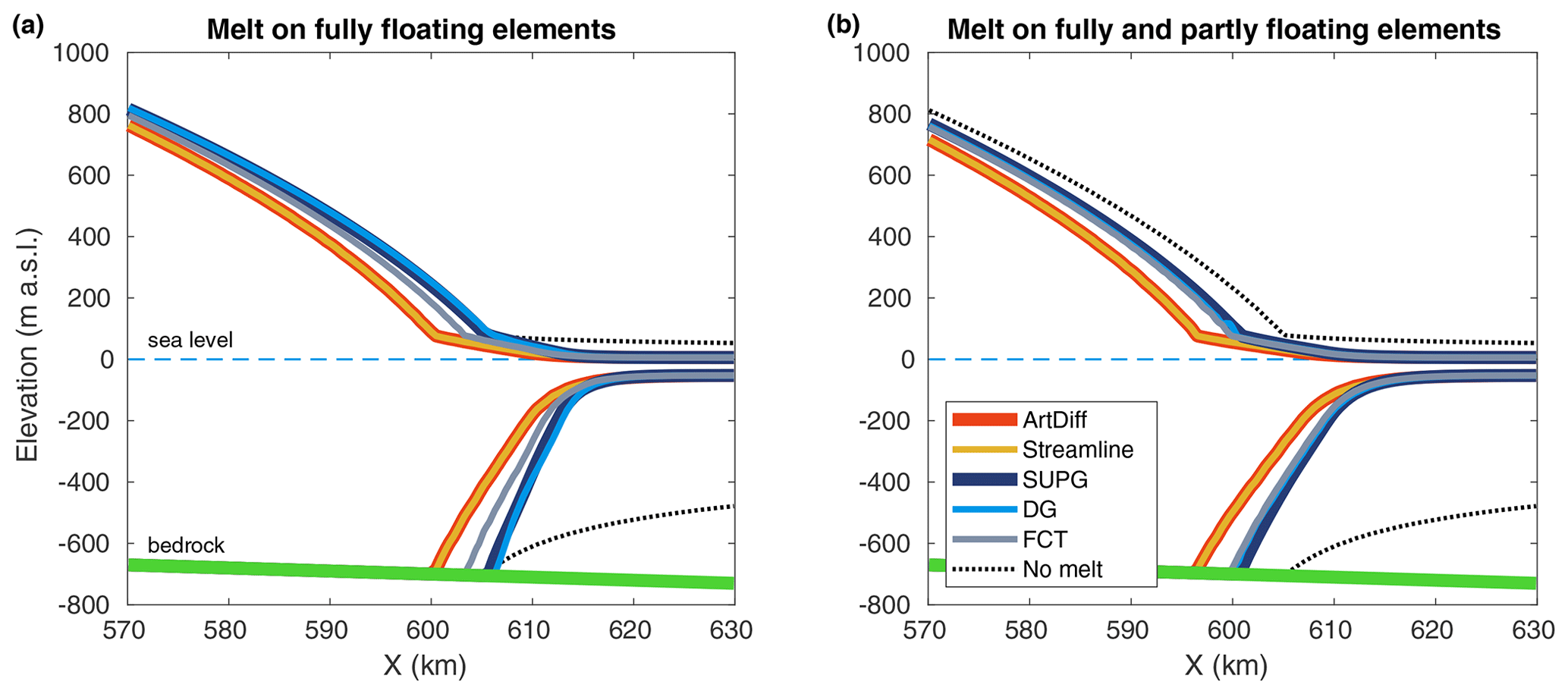
Figure 9Basal melt experiment: ice surface and ice base at the end of the experiment (t=100 years) for different stabilization schemes (see legend). (a) No melt on partly floating elements. (b) Melt on fully and partly floating elements. The dotted black line is the profile obtained with no basal melt applied (no external forcing experiment; Sect. 5.2.1 and Fig. 4). Here, the set of parameterizations is SEP1 + NSED, and the mesh resolution is equal to 500 m.
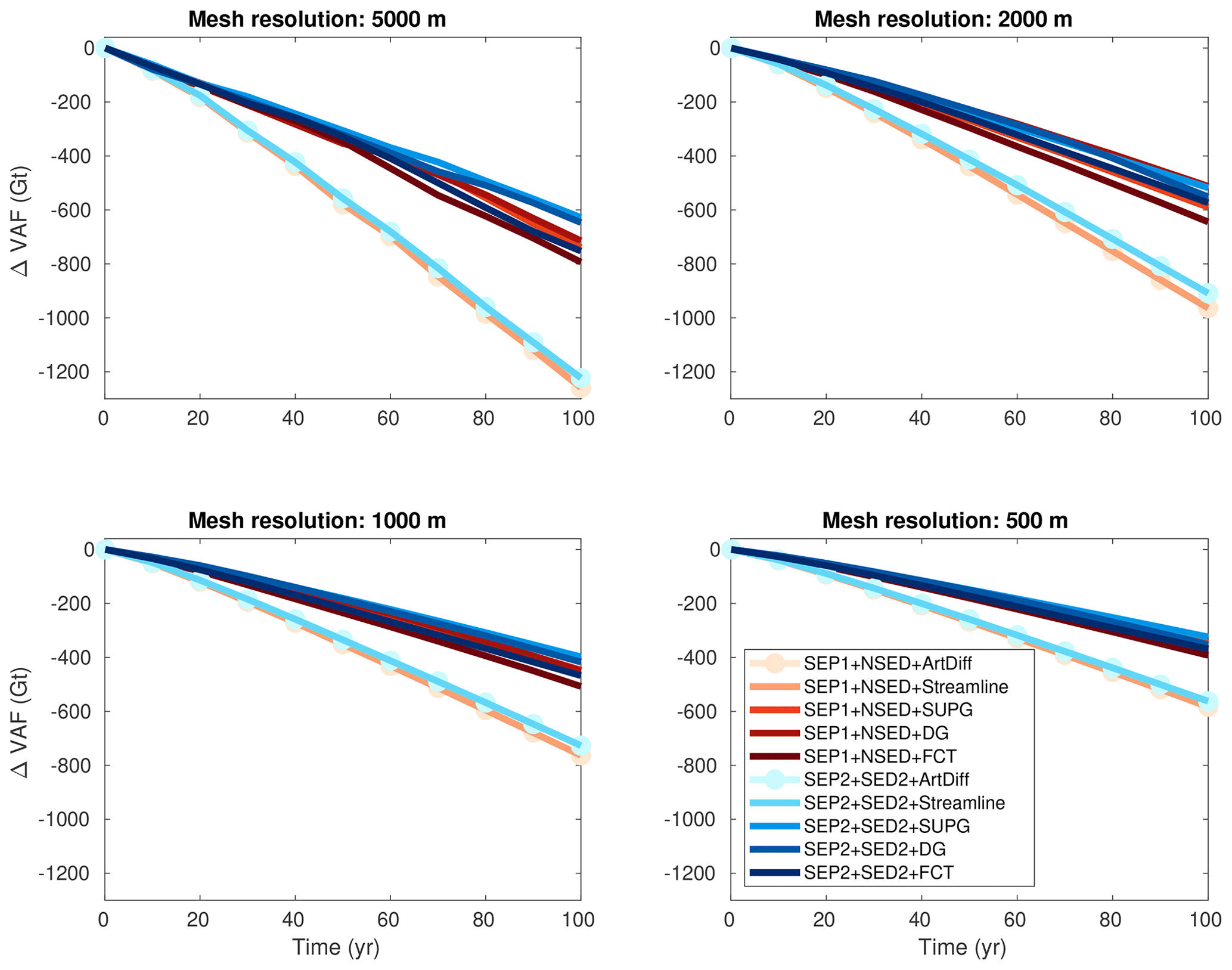
Figure 10Basal melt experiment (melt on partly floating elements): evolution of ΔVAF for different mesh resolutions and stabilization schemes (see legend). Two sets of sub-element parameterizations are employed: SEP1 + NSED and SEP2 + SED2.
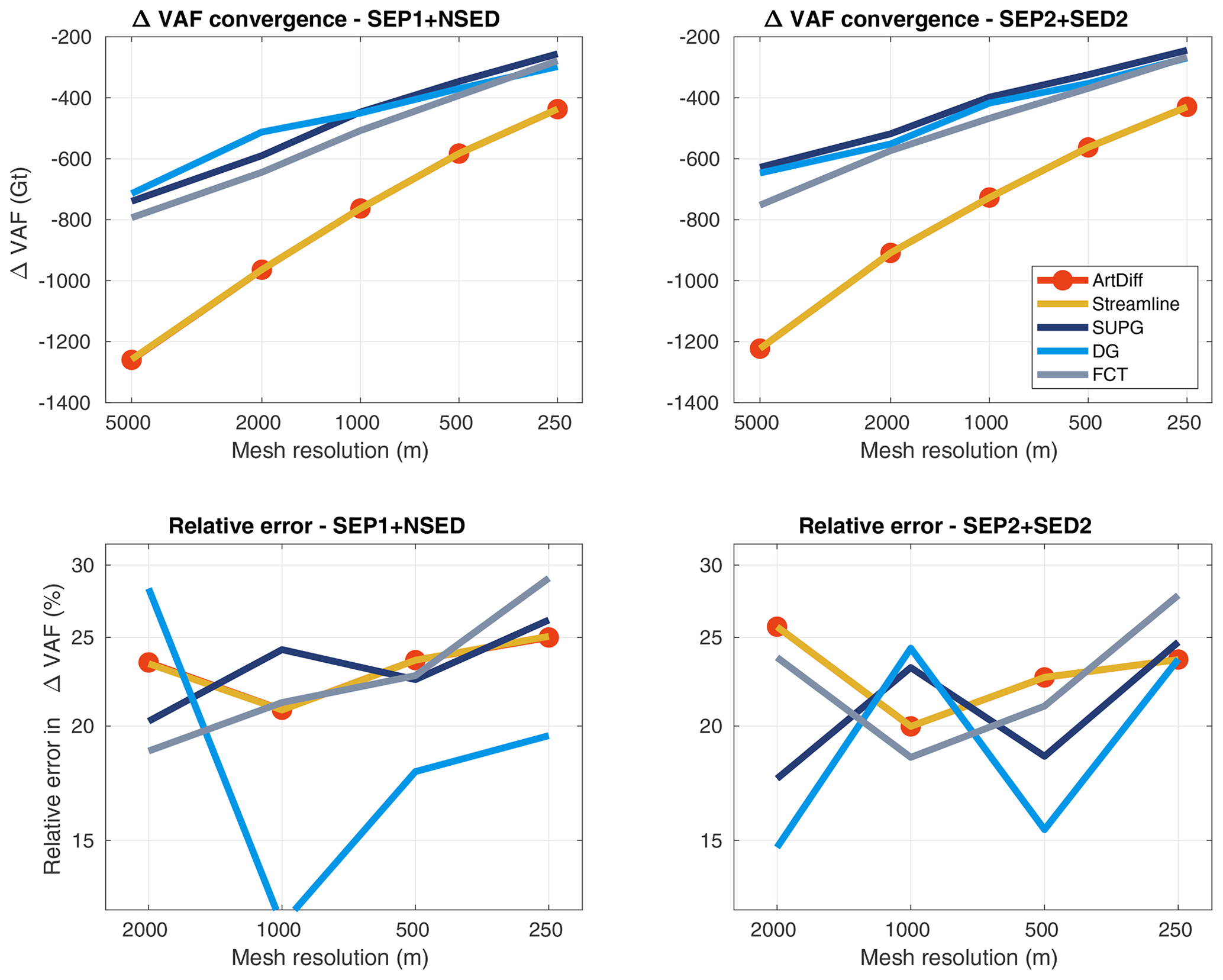
Figure 11Basal melt experiment (melt on partly floating elements): convergence of ΔVAF at the end of the experiment (t=100 years) for different stabilization schemes (see legend). Two sets of sub-element parameterizations are employed: SEP1 + NSED (left panels) and SEP2 + SED2 (right panels). The relative errors are computed using Eq. (45).
When some basal melt is also applied to partly floating elements, all models generate VAF losses higher than those generated with the previous basal melt setup (Fig. 10), as expected (Seroussi and Morlighem, 2018). Models employing artificial diffusion and streamline upwinding schemes produce almost twice the change in VAF compared to models using SUPG and discontinuous Galerkin. In this setup, FCT tends to perform as well as SUPG and discontinuous Galerkin as the mesh resolution becomes finer (Figs. 10 and 11). The grounding lines obtained with artificial diffusion and streamline upwinding schemes evolve upstream of the grounding lines computed with the SUPG, discontinuous Galerkin, and FCT schemes (Fig. 9b). The sensitivity to mesh resolution is higher for models using artificial diffusion and streamline upwinding: VAF losses vary from 400 to 1300 Gt for the range of mesh resolutions used in this study, 250 to 5000 m (Fig. 11). For models employing SUPG, discontinuous Galerkin, and FCT, VAF losses vary from about 200 to 800 Gt for the same range of mesh resolutions. In this melt setup, a mesh resolution equal to 250 m is not enough to achieve relatively small errors in VAF changes: the relative errors for this mesh resolution vary from 20 % to 30 %, depending on the stabilization scheme used, and they do not seem to have entered the asymptotic region (Fig. 11). Both sets of sub-element parameterizations, SEP1 + NSED and SEP2 + SED2, generate virtually the same ΔVAF convergence for all stabilization schemes (see Fig. 11).
5.2.3 Friction perturbation experiment
Virtually all stabilization schemes produce the same ΔVAF evolution for both sets of sub-element parameterizations (Fig. 12). The amount of mass loss at the end of the experiment varies with mesh resolution: from 1300 to 1600 Gt for the range of mesh resolutions considered here, 5000 to 250 m. Using the SUPG, discontinuous Galerkin, and FCT schemes, the models produce slightly less mass loss than artificial diffusion and streamline upwinding, ∼40 Gt (Fig. 13). Both sets of parameterizations generate similar ΔVAF convergence for all stabilization schemes (Fig. 13). For mesh resolutions equal to or finer than 1 km, the relative errors decrease to values below 5 %, reaching ∼0.5 % for a resolution of 250 m. The positions of the grounding line along the lateral boundaries (i.e., y=0 and y=50 km) reach 618 and 600.3 km, respectively, for mesh resolutions finer than 1 km (Fig. 14). For these mesh resolutions, the relative errors are smaller than 0.1 % (Fig. 15).

Figure 12Basal friction perturbation experiment: evolution of ΔVAF for different mesh resolutions and stabilization schemes (see legend). Two sets of sub-element parameterizations are employed: SEP1 + NSED and SEP2 + SED2.
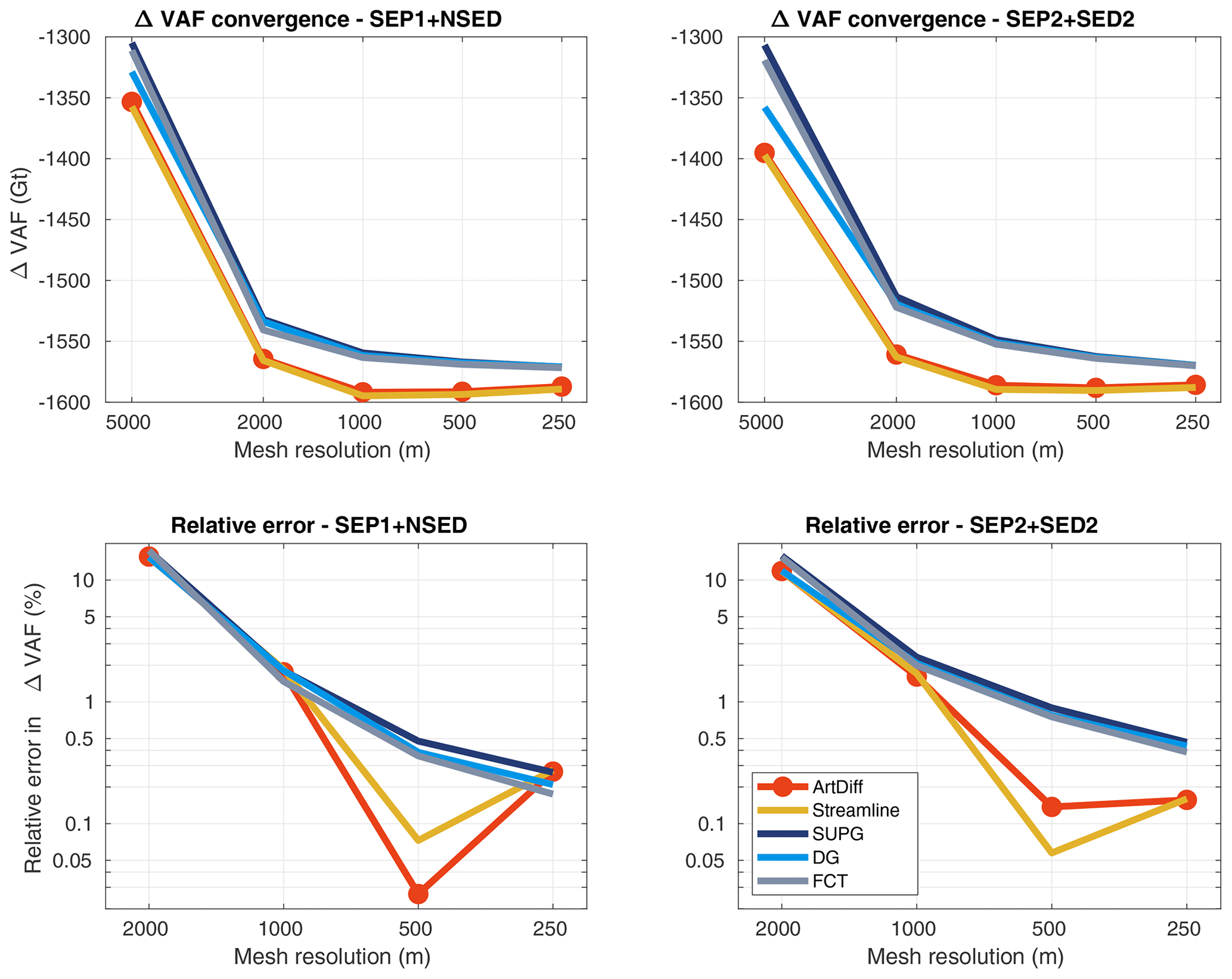
Figure 13Basal friction perturbation experiment: convergence of ΔVAF at the end of the experiment (t=100 years) for different stabilization schemes (see legend). Two sets of sub-element parameterizations are employed: SEP1 + NSED (left panels) and SEP2 + SED2 (right panels). The relative errors are computed using Eq. (45).
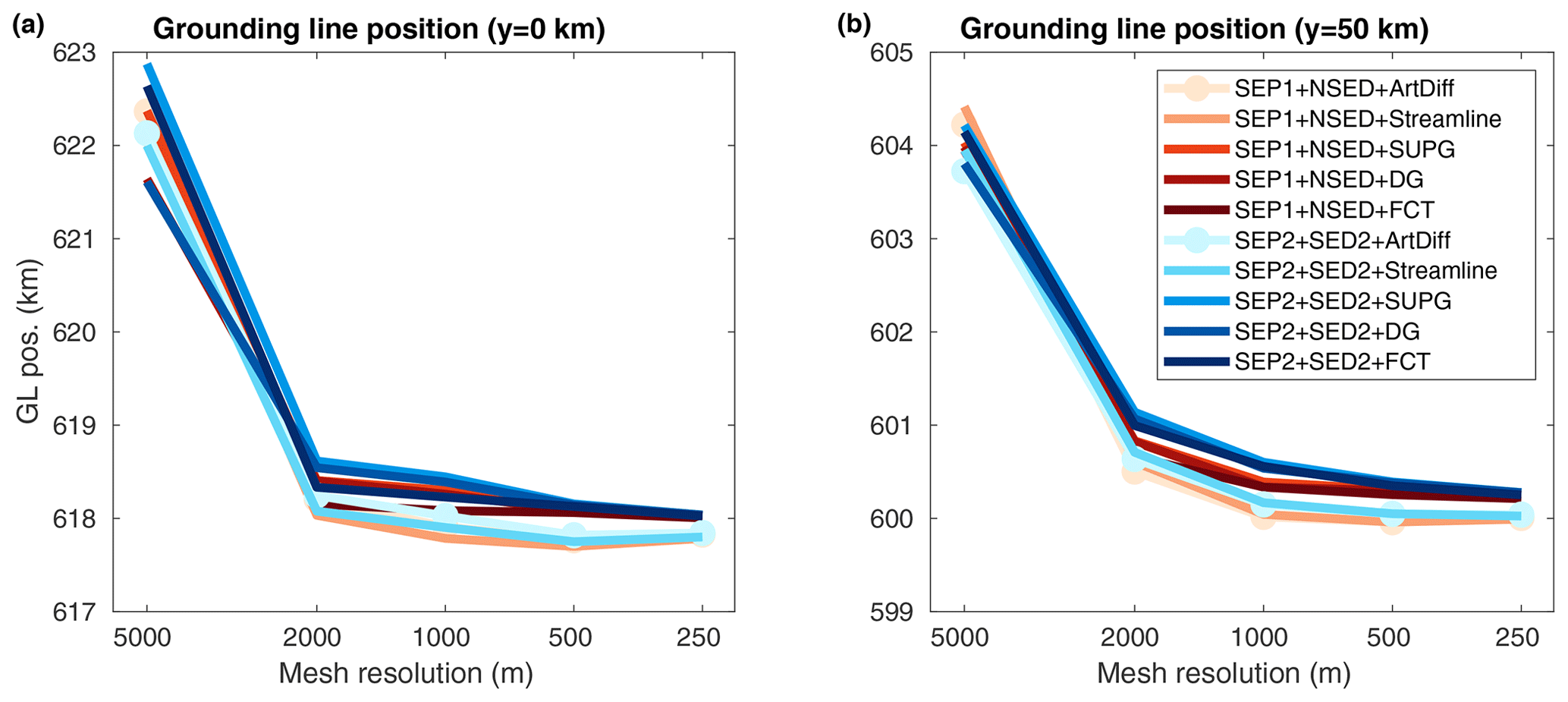
Figure 14Basal friction perturbation experiment: convergence of grounding line positions at the end of the experiment (t=100 years) for y=0 (a) and y=50 km (b). Different stabilization schemes and two sets of sub-element parameterizations are employed (see legend).
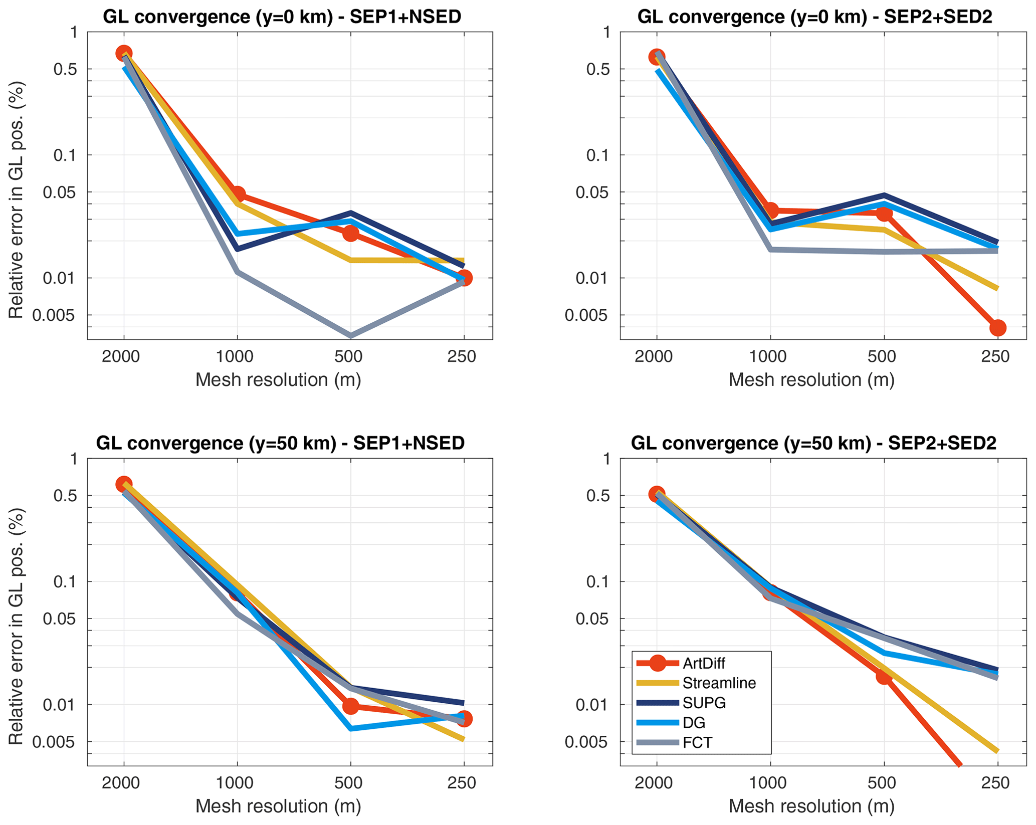
Figure 15Basal friction perturbation experiment: convergence of grounding line positions (relative errors) at the end of the experiment (t=100 years) for y=0 (top panels) and y=50 km (bottom panels) and for different stabilization schemes (see legend). Two sets of sub-element parameterizations are employed: SEP1 + NSED (left panels) and SEP2 + SED2 (right panels). The relative errors are computed using Eq. (45) and replacing ΔVAF by the grounding line position.
5.3 Amundsen Sea Embayment – prognostic analysis
To evaluate the performance of the stabilization schemes in real ice-sheet simulations (i.e., the ASE setup), we compare the VAF changes obtained with transient simulations employing the five schemes considered in this work. For the SUPG scheme, we chose the stability parameter as defined by Eq. (14). Models running with the other definition (i.e., Eq. 11) present spurious oscillations in this experiment. The two major glaciers in ASE, i.e., the Thwaites and Pine Island (PIG) glaciers, may respond differently to ocean-induced melt: Pine Island presents a more confined ice shelf compared to Thwaites. Therefore, we also compute the changes in VAF for these two glaciers.
In the experiment forced by the first basal melt scenario (i.e., m yr−1), the VAF loss after 50 years varies from 3200 to 2800 Gt for Thwaites and from 1900 to 1700 for Pine Island (Fig. 16, upper panels). In both glaciers, the artificial diffusion scheme overestimates the amount of VAF loss up to 10 % in comparison to the SUPG scheme. Discontinuous Galerkin and SUPG produce a smaller change in VAF, while streamline upwinding and FCT lies in between.
Under a higher basal melt scenario ( m yr−1), the VAF losses vary from 4400 to 3900 Gt and from 5100 to 3500 Gt for Thwaites and Pine Island, respectively (Fig. 16, lower panels). For Thwaites, the streamline upwinding scheme produces less mass loss during the entire simulation time, while artificial diffusion and FCT generate the highest amount of mass losses. The effect of the artificial damping is more pronounced in Pine Island: at the end of the experiment, the artificial diffusion scheme leads to ∼50 % more VAF loss compared to SUPG, the scheme that produces the lowest change in VAF for PIG. Discontinuous Galerkin generates spurious oscillations in ice thickness for this experimental setup, and therefore it is not shown in Fig. 16.
Considering the entire ASE domain, in simulations forced by a low melt rate ( m yr−1), the model running with artificial diffusion overestimates by 10 % the VAF loss in comparison to the one employing SUPG (Fig. 17). Under a higher rate of basal melt ( m yr−1), the VAF loss of ASE is overestimated by about 20 % in the same artificial diffusion–SUPG rate comparison (see Fig. 17). Streamline upwinding and FCT present similar responses for both melt scenarios: these schemes generate less VAF losses in comparison to artificial diffusion. This difference is more pronounced in the experiment forced by 200 m yr−1 of melt rate.

Figure 16ΔVAF along transient simulations for Thwaites (left panels) and Pine Island (PIG, right panels) glaciers. The transient simulations are forced by two different basal melt rate scenarios: 50 m yr−1 (upper panels) and 200 m yr−1 (lower panels). The basal melt is applied only on fully floating elements, and the parameterization schemes for basal friction and driving stress are SEP1 and NSED, respectively.
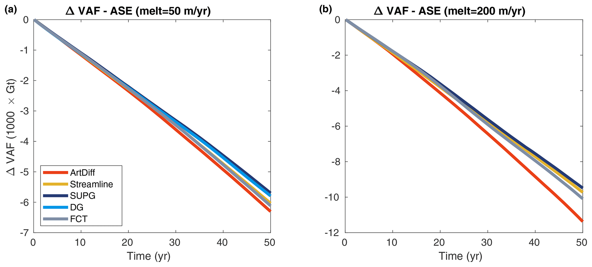
Figure 17ΔVAF along transient simulations for the Amundsen Sea Embayment (ASE) domain. The transient simulations are forced by two different basal melt rate scenarios: 50 m yr−1 (a) and 200 m yr−1 (b). The basal melt is applied only on fully floating elements, and the parameterization schemes for basal friction and driving stress are SEP1 and NSED, respectively.
The diagnostic analysis using the analytical ice-sheet profile (Sect. 5.1) shows that the convergence of ice speeds depends on the set of parameterizations chosen. The convergence curve associated with the new driving stress parameterization (SED2) is similar to the ones of structured conforming meshes when combined with the parameterization SEP2 for basal friction. Specifically, considering an a priori error estimate of khβ, where k and β are constants, k is independent of h, β depends on the polynomial order of elements and smoothness of the solution (Szabó and Babuška, 1991, p. 61, 62), employing SEP2 + SED2 reduces the value of k to a value closer to the ones produced by structured conforming meshes (see SEP2 + SED2 and SEP2 + NSED in Fig. 3). The same is observed for SEP1 + NSED in comparison to SEP1 + SED2. Overall, models employing SEP1 + NSED and SEP2 + SED2 achieve relatively low levels of errors with mesh resolutions at least 4 times coarser in comparison to the other schemes, SEP1 + SED2 and SEP2 + NSED (see Fig. 3). These results suggest that improved convergence (i.e., smaller k) is achieved by discretizing consistently the friction coefficient and driving stress, i.e., by employing SEP1 + NSED or SEP2 + SED2. This is consistent with previous studies based on finite-volume and finite-difference methods (Cornford et al., 2013; Feldmann et al., 2014), where one-sided differences were employed on each side of the grounding line to compute surface gradients and basal friction. The driving stress and basal friction should be equally balanced (i.e., discretized) at the grounding line to improve the accuracy of the ice velocity as well as the dynamics of the grounding line (Cornford et al., 2013; Feldmann et al., 2014). The error norms for fine mesh resolutions (500 m or finer) shown in Fig. 3 are probably impacted by our iterative solver. However, note that the errors for these mesh resolutions are below 1 m yr−1 in the L∞ norm, or m s−1, which is the same order of magnitude as our solver tolerance and machine precision.
Table 4Steady-state GL positions for the MISMIP3d setup using different sub-element parameterization schemes. GL positions for SEP1 + NSED and SEP2 + NSED are extracted from Seroussi et al. (2014a). We employ the same numerical setup as described in Seroussi et al. (2014a). The estimated GL position from BLT is also included (Schoof, 2007b).
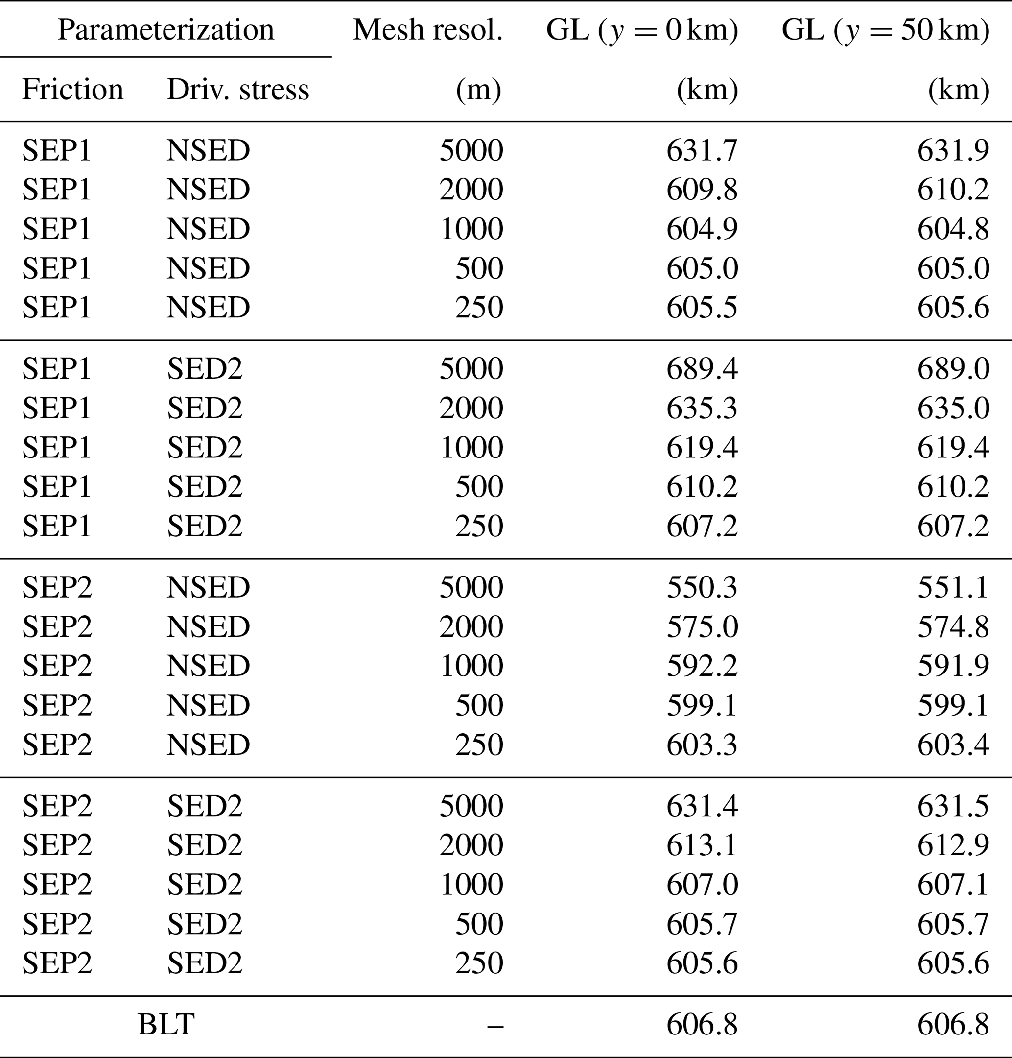
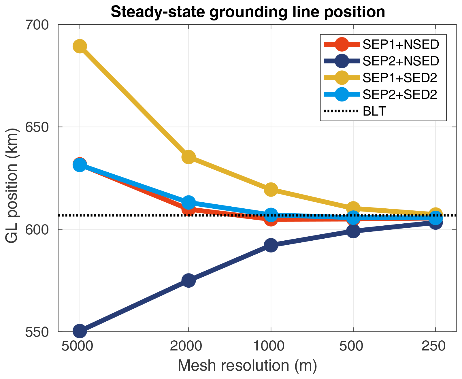
Figure 18Convergence of steady-state grounding line (GL) positions (y=0 km) for the MISMIP3d setup. Different sets of sub-element parameterizations are tested: SEP1 + NSED, SEP2 + NSED, SEP1 + SED2, and SEP2 + SED2. The dotted line is the grounding position from the boundary layer theory (BLT) (Schoof, 2007b).
Employing an analytical expression of ice geometry based on a predefined grounding line position allows the setup of reference models (i.e., models whose mesh captures the exact position of the grounding line), in which no errors due to parameterization schemes are introduced during the stress balance solution (diagnostic analysis). Therefore, using the reference setup improves the confidence of this analysis. Comparing grounding line positions at steady state is another approach (Table 4 and Fig. 18) where the boundary layer theory (BLT) provides an estimated position of the steady grounding line. The steady-state comparison shows that 1 km mesh resolution is enough for models using SEP1 + NSED and SEP2 + SED2 to achieve the grounding line position predicted by the BLT, within a tolerance of 0.5 %, while models employing other schemes (SEP1 + SED2 and SEP2 + NSED) need finer mesh resolution (at least 16 times more elements to generate a 250 m resolution mesh) to achieve the BLT prediction with the same tolerance. This corroborates the conclusions obtained with the diagnostic analysis in Sect. 5.1.
The prognostic analysis performed with the MISMIP3d-type geometry shows that the numerical damping produced by the artificial diffusion and streamline upwinding schemes impacts the accuracy of grounding line dynamics mainly in simulations when large ΔH appear at its vicinity, such as the ice-shelf melt experiments. These two schemes generate the same stabilization term in the x-direction flow performed in this numerical setup (see Sect. 2.2). The numerical damping induces a positive feedback of mass loss: the grounded ice upstream of the grounding line thins due to the (artificial) damping and starts to unground; once it is floating, it is subject to basal melt, which induces further thinning inland. For melt-induced experiments, where some melt is also applied to partly floating elements, models running with artificial diffusion and streamline upwinding overestimate mass loss in comparison to models running with other schemes (SUPG, DG, and FCT). Note, however, that applying melt on partly floating elements leads to high levels of errors for all the stabilization schemes and mesh resolutions used in this study and therefore is not a suitable approach. The basal friction perturbation experiment (Sect. 5.2.3) shows that, for a given mesh resolution, the relative errors in ΔVAF are at least 1 order of magnitude higher than the errors in grounding line position (see Figs. 13 and 15). For instance, the grounding line position has an error of 1 % for a 2 km mesh, while the corresponding error in ΔVAF is higher than 10 %. Small changes in grounding line position can therefore lead to large differences in ΔVAF. This suggests that ΔVAF should be used as a metric of numerical convergence in ice-sheet model intercomparison projects. The MISMIP3d setup used in this analysis is suitable because (1) there is no buttressing effect involved in these basal melt experiments, and therefore the grounding line dynamics is expected to be independent of ice-shelf basal melt; (2) the bedrock is the same for all mesh resolutions, which eliminates the source of errors related to bedrock resolution (Durand et al., 2011); (3) it allows the definition of an analytical ice-sheet profile and guarantees the same initial condition for all models independently of the mesh resolution or stabilization schemes. These numerical characteristics therefore eliminate the influence of several sources of errors, allowing the analysis to focus only on the response to the stabilization schemes.
For the prognostic analysis performed with real glaciers in West Antarctica (Sect. 5.3), streamline upwinding performs as well as the FCT scheme, which may be explained by the “anisotropic balancing dissipation” of the stabilization term (Kelly et al., 1980; Brooks and Hughes, 1982) (Sect. 2.2) that has prevented numerical damping over transverse flows. Interestingly, streamline upwinding generates less mass loss in comparison to SUPG for the Thwaites Glacier in the high-melt-rate scenario (Fig. 16). We attribute this to the low performance of the stabilization parameter (τ) in this simulation. In this same melt scenario, the mass loss of PIG is clearly overestimated using artificial diffusion, which is likely associated with the positive feedback explained above: the grounding line of PIG retreats several kilometers more using ArtDiff compared to the other schemes. For the entire ASE domain considered here, SUPG, FCT, and streamline upwinding yield similar VAF evolution within a difference of ∼5 % in the high-melt experiment. Discontinuous Galerkin has similar performance to SUPG, at least for the lower-basal-melt scenario. However, producing spurious oscillations in ice thickness in the second melt experiment highlights that the DG scheme as implemented in ISSM may be not completely robust.
The choice of the stabilization scheme relies on the balance between stability, accuracy, computational cost, and implementation effort. Yet, the “best” choice could be never reached (e.g., John et al., 2018). Artificial diffusion provides stability to numerical solutions, even in the presence of strong discontinuities and shocks (which is not the case in ice-sheet dynamics). But at the same time, it excessively smooths the solution for large ΔH, which impacts the results. For simulations with large buttressing effect, as is the case for the Pine Island and Thwaites glaciers, numerical damping could artificially “enhance” the marine ice-sheet instability feedback existing for retrograde bedrock slopes and, consequently, overestimate mass loss in ocean-induced melt simulations. Note that numerical damping does not always lead to grounding line retreat, but it can also prevent its advance. High mesh resolution could be employed to decrease the diffusion effects, but it comes at a higher computational cost. Adaptive mesh refinement could be an alternative in this case, although it is not available in all ice-sheet models. Discontinuous Galerkin and SUPG may generate spurious oscillations in idealized experiments where discontinuities are present (e.g., John and Schmeyer, 2008), and in real ice-sheet simulations, as observed here for ASE experiments. The performance and stability of SUPG clearly rely on the definition of the stabilization parameter τ, and the numerical issues and results observed here for the ASE simulations indicate that the definitions of τ as given by Eqs. (11) and (14) are not totally robust and optimized for real ice-sheet simulations, at least for the SUPG as currently implemented in ISSM. FCT presents better results on idealized cases (John and Schmeyer, 2008), but some excessive VAF loss is observed in some experiments performed here (e.g., Fig. 7). Besides that, this scheme performs as well as the streamline upwinding in the two basal melt scenarios using the ASE setup.
Apart from differences observed in terms of accuracy (i.e., VAF change), the remaining differences between the stabilization schemes used here are their numerical implementations and computational costs. The implementation of the artificial diffusion, streamline upwinding, and SUPG is straightforward in most of ice-sheet FEM-based models. However, the definition of the stability coefficient for SUPG (Eq. 7) is problem dependent, and possibly, its optimum value may remain unclear in many real ice-sheet simulations. Discontinuous Galerkin requires specific coding of data structures, at the minimum requiring information on elements' neighbors, and significant implementation effort to compute the integrals along elements' edges. Also, the number of degrees of freedom in comparison to other schemes is considerably increased (up to a factor of 6 for triangular P1 Lagrange elements), which impacts the computational cost when the backward Euler approach is used, as is the case in ISSM. An alternative would be an explicit approach (Runge–Kutta discontinuous Galerkin): in this case, the solution using the DG scheme would be completely parallel (e.g., Cockburn, 2003). While this would improve the computational cost, there are more stringent restrictions on the CFL time step. The FCT scheme requires operations on global matrices and vectors. While this is straightforward in codes relying on shared memory (e.g., one process, multiple threads), these operations require additional CPU communications in codes based on distributed memory (e.g., Message Passing Interface), potentially translating into a larger computation time. Finally, we note that the current ISSM implementations of the stabilization schemes presented here are based on the classical literature of FEM, where the numerical analyses of such schemes are carried out in idealized problems. There is still room for development of stabilization schemes and improved numerical accuracy, stability, and computational performance in the specific field of ice-sheet modeling; most stabilization schemes were designed to handle the presence of shocks and strong discontinuities, which are mostly absent from this field.
The convergence error of ice speed depends on the combination of parameterizations chosen for basal friction and driving stress. Given that the a priori error estimate is khβ (h is the mesh resolution), the sub-element parameterization for driving stress proposed here (SED2) presents smaller values of k when combined with a similar approach for basal friction (SEP2). In models employing the SEP1 basal friction parameterization, a smaller k is achieved with no driving stress parameterization (NSED). As already suggested by previous simulations based on finite-volume or finite-difference methods, in order to achieve improved numerical convergence (i.e., smaller values of k) for a given computational cost, the discretization of the basal friction should match the discretization of the driving stress; the following combinations of sub-element parameterizations therefore provide the best results: SEP1 + NSED and SEP2 + SED2. In all transient simulations performed here for both idealized and real ice-sheet configurations, models relying on artificial diffusion generate the largest amount of mass loss in comparison to models running with the other schemes. SUPG and discontinuous Galerkin produce the expected grounding line dynamics for the idealized case (e.g., MISMIP3d-type setup). For the ASE experiments, these two schemes produce less mass loss than the others ones, although some spurious oscillations are observed, which compromised the results. By design, the streamline upwinding has the same behavior as artificial diffusion in the idealized case (x-direction flow). However, in the real ice-sheet simulations (ASE setup), streamline upwinding performs as well as the flux-corrected transport scheme. Based on the numerical tests performed here and the ease of implementation, SUPG seems a preferred scheme, although careful attention shall be given to the definition of the stabilization parameter, which may be problem dependent. A second choice would be the streamline upwinding scheme, as long as a high-enough mesh resolution is employed around the discontinuities (e.g., grounding line). The development of new stabilization schemes and/or improvements of existing ones in FEM remains an active field of research. Nevertheless, since most theoretical studies and convergence analyses involve, in general, smooth data and regular boundaries, the conclusions drawn from these studies may not necessarily hold for real cases, such as the Amundsen Sea Embayment simulation performed here. This highlights the importance of testing future stabilization schemes with real geometries and external forcing. In general, most stabilization schemes were developed in the context of compressible flow, where shocks and strong discontinuities appear, which is not the case of ice-sheet modeling, opening new development opportunities for this specific field.
Six examples of structured and unstructured meshes are shown in Fig. B1. We use the package Triangle (Shewchuk, 1996) to generate the unstructured meshes.
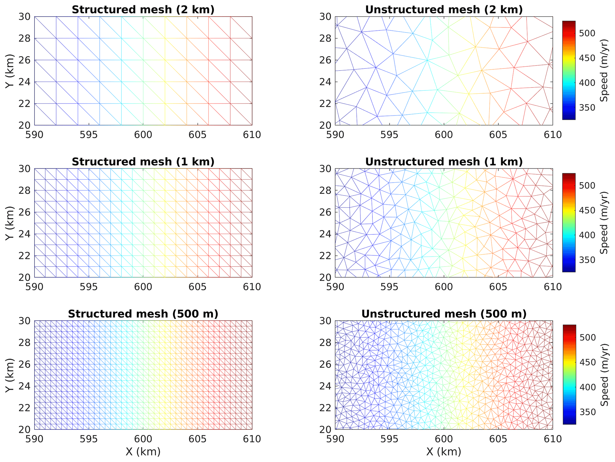
Figure B1Examples of meshes employed in this work. Left panels are structured conforming meshes, and right panels the unstructured meshes. Three mesh resolutions are shown: 2, 1, and 0.5 km. The color maps are the ice speeds obtained in the diagnostic analysis (Sect. 5.1) considering the grounding line at x=600 km. Note that the structured meshes are conforming to the grounding line; i.e., they are generated such that the elements' edges match the grounding line position (in this case, xgl=600 km). Sub-element parameterizations SEP1 + NSED are employed in the unstructured meshes to computed the ice speeds presented here.
The numerical schemes evaluated here are currently implemented in the ISSM. The code can be downloaded, compiled, and executed following the instructions available on the ISSM website: https://issm.jpl.nasa.gov/download (last access: 20 November 2020). The public SVN repository for the ISSM code can also be found directly at https://issm.ess.uci.edu/svn/issm/issm/trunk (Larour et al., 2020) and downloaded using username “anon” and password “anon”. The version of the code for this study, corresponding to ISSM release 4.18, is SVN version tag number 25833. The documentation of the code version used here is available at https://issm.jpl.nasa.gov/documentation/ (last access: 20 November 2020).
All data sets used in the prognostic analysis of the Amundsen Sea Embayment, Sects. 4.2 and 5.3, are freely available in the public domain and are referenced in the text. BedMachine Antarctica v1 is available at the National Snow and Ice Data Center (NSIDC), Boulder, CO, https://doi.org/10.5067/C2GFER6PTOS4 (Morlighem, 2019). The InSAR-derived surface velocity is available at the NSIDC, Boulder, CO, https://doi.org/10.5067/PZ3NJ5RXRH10 (Mouginot et al., 2019b).
The supplement related to this article is available online at: https://doi.org/10.5194/gmd-14-2545-2021-supplement.
MM and HS implemented some stabilization schemes in ISSM. TDS implemented the driving stress parameterization and stabilization SUPG. TDS designed the experimental setup and performed the simulations. TDS, MM, and HS led the analysis of the results. TDS led the initial writing of the paper. All authors contributed to writing the final version of the paper.
The authors declare that they have no conflict of interest.
This work is from the PROPHET project, a component of the International Thwaites Glacier Collaboration (ITGC). Support comes from the National Science Foundation. This is ITGC contribution no. ITGC-022. Hélène Seroussi is funded by grants from the NASA Cryospheric Sciences Program. We thank the editor, Steven Phipps, and the two reviewers, Stephen Cornford and Daniel Martin, for their positive and constructive comments, which improved the clarity of the manuscript.
This research has been supported by the National Science Foundation (grant no. 1739031).
This paper was edited by Steven Phipps and reviewed by Stephen Cornford and Daniel Martin.
Akin, J. and Tezduyar, T. E.: Calculation of the advective limit of the SUPG stabilization parameter for linear and higher-order elements, Comput. Method. Appl. M., 193, 1909–1922, https://doi.org/10.1016/j.cma.2003.12.050, 2004. a
Almeida, R. C. and Silva, R. S.: A stable Petrov–Galerkin method for convection-dominated problems, Comput. Method. Appl. M., 140, 291–304, https://doi.org/10.1016/S0045-7825(96)01108-5, 1997. a
Arnold, D. N., Brezzi, F., Cockburn, B., and Marini, L. D.: Unified Analysis of Discontinuous Galerkin Methods for Elliptic Problems, SIAM J. Numer. Anal., 39, 1749–1779, https://doi.org/10.1137/S0036142901384162, 2002. a
Aschwanden, A., Fahnestock, M. A., Truffer, M., Brinkerhoff, D. J., Hock, R., Khroulev, C., Mottram, R., and Khan, S. A.: Contribution of the Greenland Ice Sheet to sea level over the next millennium, Science Advances, 5, eaav9396, https://doi.org/10.1126/sciadv.aav9396, 2019. a
Babuška, I., Baumann, C., and Oden, J.: A discontinuous hp finite element method for diffusion problems: 1-D analysis, Comput. Math. Appl., 37, 103–122, https://doi.org/10.1016/S0898-1221(99)00117-0, 1999. a
Barnes, J. M., dos Santos, T. D., Goldberg, D., Gudmundsson, G. H., Morlighem, M., and De Rydt, J.: The transferability of adjoint inversion products between different ice flow models, The Cryosphere Discuss. [preprint], https://doi.org/10.5194/tc-2020-235, in review, 2020. a
Blank, H., Rudgyard, M., and Wathen, A.: Stabilised finite element methods for steady incompressible flow, Comput. Method. Appl. M., 174, 91–105, https://doi.org/10.1016/S0045-7825(98)00279-5, 1999. a
Blatter, H.: Velocity and stress-fields in grounded glaciers: A simple algorithm for including deviatoric stress gradients, J. Glaciol., 41, 333–344, 1995. a
Bochev, P. B., Gunzburger, M. D., and Shadid, J. N.: Stability of the SUPG finite element method for transient advection–diffusion problems, Comput. Method. Appl. M., 193, 2301–2323, https://doi.org/10.1016/j.cma.2004.01.026, 2004. a
Boris, J. P. and Book, D. L.: Flux-corrected transport. I. SHASTA, a fluid transport algorithm that works, J. Comput. Phys., 11, 38–69, https://doi.org/10.1016/0021-9991(73)90147-2, 1973. a
Brezzi, F., Manzini, G., Marini, D., Pietra, P., and Russo, A.: Discontinuous Galerkin approximations for elliptic problems, Numer. Meth. Part. D. E., 16, 365–378, https://doi.org/10.1002/1098-2426(200007)16:4<365::AID-NUM2>3.0.CO;2-Y, 2000. a
Brezzi, F., Marini, L. D., and Süli, E.: Discontinuous Galerkin methods for first-order hyperbolic problems, Math. Mod. Meth. Appl. S., 14, 1893–1903, https://doi.org/10.1142/S0218202504003866, 2004. a, b
Brooks, A. N. and Hughes, T. J.: Streamline upwind/Petrov–Galerkin formulations for convection dominated flows with particular emphasis on the incompressible Navier–Stokes equations, Comput. Method. Appl. M., 32, 199–259, https://doi.org/10.1016/0045-7825(82)90071-8, 1982. a, b, c, d, e, f, g, h
Burman, E.: Consistent SUPG-method for transient transport problems: Stability and convergence, Comput. Method. Appl. M., 199, 1114–1123, https://doi.org/10.1016/j.cma.2009.11.023, 2010. a
Calle, J. L., Devloo, P. R., and Gomes, S. M.: Stabilized discontinuous Galerkin method for hyperbolic equations, Comput. Method. Appl. M., 194, 1861–1874, https://doi.org/10.1016/j.cma.2004.06.036, 2005. a
Christie, I., Griffiths, D. F., Mitchell, A. R., and Zienkiewicz, O. C.: Finite element methods for second order differential equations with significant first derivatives, Int. J. Numer. Meth. Eng., 10, 1389–1396, https://doi.org/10.1002/nme.1620100617, 1976. a
Cockburn, B.: An introduction to the Discontinuous Galerkin method for convection-dominated problems, Springer, Berlin, Heidelberg, Germany, 150–268, https://doi.org/10.1007/BFb0096353, 1998. a, b, c, d
Cockburn, B.: Discontinuous Galerkin Methods for Convection-Dominated Problems, Springer, Berlin, Heidelberg, Germany, 69–224, https://doi.org/10.1007/978-3-662-03882-6_2, 1999. a
Cockburn, B.: Discontinuous Galerkin methods, ZAMM-Z. Angew. Math. Me., 83, 731–754, https://doi.org/10.1002/zamm.200310088, 2003. a, b, c
Cockburn, B. and Shu, C.-W.: The Runge–Kutta local projection P1-discontinuous-Galerkin finite element method for scalar conservation laws, ESAIM: M2AN, 25, 337–361, https://doi.org/10.1051/m2an/1991250303371, 1991. a
Codina, R.: Comparison of some finite element methods for solving the diffusion-convection-reaction equation, Comput. Method. Appl. M., 156, 185–210, https://doi.org/10.1016/S0045-7825(97)00206-5, 1998. a, b
Codina, R.: On stabilized finite element methods for linear systems of convection–diffusion-reaction equations, Comput. Method. Appl. M., 188, 61–82, https://doi.org/10.1016/S0045-7825(00)00177-8, 2000. a
Cornford, S. L., Martin, D. F., Graves, D. T., Ranken, D. F., Brocq, A. M. L., Gladstone, R. M., Payne, A. J., Ng, E. G., and Lipscomb, W. H.: Adaptive mesh, finite volume modeling of marine ice sheets, J. Comput. Phys., 232, 529–549, https://doi.org/10.1016/j.jcp.2012.08.037, 2013. a, b, c, d, e
Cornford, S. L., Martin, D. F., Payne, A. J., Ng, E. G., Le Brocq, A. M., Gladstone, R. M., Edwards, T. L., Shannon, S. R., Agosta, C., van den Broeke, M. R., Hellmer, H. H., Krinner, G., Ligtenberg, S. R. M., Timmermann, R., and Vaughan, D. G.: Century-scale simulations of the response of the West Antarctic Ice Sheet to a warming climate, The Cryosphere, 9, 1579–1600, https://doi.org/10.5194/tc-9-1579-2015, 2015. a
Cornford, S. L., Martin, D. F., Lee, V., Payne, A. J., and Ng, E. G.: Adaptive mesh refinement versus subgrid friction interpolation in simulations of Antarctic ice dynamics, Ann. Glaciol., 57, 1–9, https://doi.org/10.1017/aog.2016.13, 2016. a
Cuffey, K. and Paterson, W. S. B.: The Physics of Glaciers, 4th edn., Elsevier, Oxford, 2010. a, b
de Vahl Davis, G. and Mallinson, G.: An evaluation of upwind and central difference approximations by a study of recirculating flow, Comput. Fluids, 4, 29–43, https://doi.org/10.1016/0045-7930(76)90010-4, 1976. a
DeConto, R. M. and Pollard, D.: Contribution of Antarctica to past and future sea-level rise, Nature, 531, 591–597, https://doi.org/10.1038/nature17145, 2016. a
Devloo, P., Forti, T., and Gomes, S.: A combined continuous-discontinuous finite element method for convection-diffusion problems, Lat. Am. J. Solids Stru., 4, 229–246, 2007. a
Diddens, C.: Detailed finite element method modeling of evaporating multi-component droplets, J. Comput. Phys., 340, 670–687, https://doi.org/10.1016/j.jcp.2017.03.049, 2017. a
Docquier, D., Pollard, D., and Pattyn, F.: Thwaites Glacier grounding-line retreat: influence of width and buttressing parameterizations, J. Glaciol., 60, 305–313, https://doi.org/10.3189/2014JoG13J117, 2014. a
Donea, J.: A Taylor–Galerkin method for convective transport problems, Int. J. Numer. Meth. Eng., 20, 101–119, https://doi.org/10.1002/nme.1620200108, 1984a. a
Donea, J.: Recent advances in computational methods for steady and transient transport problems, Nuclear Engineering and Design, 80, 141–162, https://doi.org/10.1016/0029-5493(84)90163-8, 1984b. a
Donea, J., Giuliani, S., Laval, H., and Quartapelle, L.: Time-accurate solution of advection-diffusion problems by finite elements, Comput. Method. Appl. M., 45, 123–145, https://doi.org/10.1016/0045-7825(84)90153-1, 1984. a
Dupont, T. K. and Alley, R. B.: Assessment of the importance of ice-shelf buttressing to ice-sheet flow, Geophys. Res. Lett., 32, L04503, https://doi.org/10.1029/2004GL022024, 2005. a
Durand, G., Gagliardini, O., Zwinger, T., Le Meur, E., and Hindmarsh, R. C. A.: Full Stokes modeling of marine ice sheets: influence of the grid size, Ann. Glaciol., 50, 109–114, https://doi.org/10.3189/172756409789624283, 2009. a
Durand, G., Gagliardini, O., Favier, L., Zwinger, T., and Le Meur, E.: Impact of bedrock description on modeling ice sheet dynamics, Geophys. Res. Lett., 38, 1–6, https://doi.org/10.1029/2011GL048892, 2011. a
Favier, L., Durand, G., Cornford, S. L., Gudmundsson, G. H., Gagliardini, O., Gillet-Chaulet, F., Zwinger, T., Payne, A. J., and Le Brocq, A. M.: Retreat of Pine Island Glacier controlled by marine ice-sheet instability, Nat. Clim. Change, 4, 117–121, https://doi.org/10.1038/nclimate2094, 2014. a
Feldmann, J., Albrecht, T., Khroulev, C., Pattyn, F., and Levermann, A.: Resolution-dependent performance of grounding line motion in a shallow model compared with a full-Stokes model according to the MISMIP3d intercomparison, J. Glaciol., 60, 353–360, https://doi.org/10.3189/2014JoG13J093, 2014. a, b, c, d, e
Franca, L. P., Hauke, G., and Masud, A.: Revisiting stabilized finite element methods for the advective–diffusive equation, Comput. Method. Appl. M., 195, 1560–1572, https://doi.org/10.1016/j.cma.2005.05.028, 2006. a, b
Gagliardini, O., Zwinger, T., Gillet-Chaulet, F., Durand, G., Favier, L., de Fleurian, B., Greve, R., Malinen, M., Martín, C., Råback, P., Ruokolainen, J., Sacchettini, M., Schäfer, M., Seddik, H., and Thies, J.: Capabilities and performance of Elmer/Ice, a new-generation ice sheet model, Geosci. Model Dev., 6, 1299–1318, https://doi.org/10.5194/gmd-6-1299-2013, 2013. a, b, c
Goelzer, H., Nowicki, S., Payne, A., Larour, E., Seroussi, H., Lipscomb, W. H., Gregory, J., Abe-Ouchi, A., Shepherd, A., Simon, E., Agosta, C., Alexander, P., Aschwanden, A., Barthel, A., Calov, R., Chambers, C., Choi, Y., Cuzzone, J., Dumas, C., Edwards, T., Felikson, D., Fettweis, X., Golledge, N. R., Greve, R., Humbert, A., Huybrechts, P., Le clec'h, S., Lee, V., Leguy, G., Little, C., Lowry, D. P., Morlighem, M., Nias, I., Quiquet, A., Rückamp, M., Schlegel, N.-J., Slater, D. A., Smith, R. S., Straneo, F., Tarasov, L., van de Wal, R., and van den Broeke, M.: The future sea-level contribution of the Greenland ice sheet: a multi-model ensemble study of ISMIP6, The Cryosphere, 14, 3071–3096, https://doi.org/10.5194/tc-14-3071-2020, 2020. a
Goldberg, D., Holland, D. M., and Schoof, C.: Grounding line movement and ice shelf buttressing in marine ice sheets, J. Geophys. Res.-Earth, 114, 1–23, https://doi.org/10.1029/2008JF001227, 2009. a
Gresho, P. M. and Lee, R. L.: Don't suppress the wiggles – they're telling you something, Tech. rep., United States, uCRL–82979, available at: http://inis.iaea.org/search/search.aspx?orig_q=RN:11526189 (last access: 25 November 2020), 1979. a
Greve, R. and Blatter, H.: Dynamics of Ice Sheets and Glaciers, Advances in Geophysical and Environmental Mechanics and Mathematics, 1st Edn., Springer, Berlin, Heidelberg, Germany, 2009. a
Griffiths, D. and Lorenz, J.: An analysis of the petrov – galerkin finite element method, Comput. Method. Appl. M., 14, 39–64, https://doi.org/10.1016/0045-7825(78)90012-9, 1978. a
Gudmundsson, G. H.: GHilmarG/UaSource: Ua2019b (Version v2019b), Zenodo [code], https://doi.org/10.5281/zenodo.3706623, 2020. a, b, c, d
Gudmundsson, G. H., Krug, J., Durand, G., Favier, L., and Gagliardini, O.: The stability of grounding lines on retrograde slopes, The Cryosphere, 6, 1497–1505, https://doi.org/10.5194/tc-6-1497-2012, 2012. a
Gudmundsson, G. H., Paolo, F. S., Adusumilli, S., and Fricker, H. A.: Instantaneous Antarctic ice sheet mass loss driven by thinning ice shelves, Geophys. Res. Lett., 46, 13903–13909, https://doi.org/10.1029/2019GL085027, 2019. a
Hansen, K. B., Arzani, A., and Shadden, S. C.: Finite element modeling of near-wall mass transport in cardiovascular flows, Int. J. Numer. Meth. Bio., 35, e3148, https://doi.org/10.1002/cnm.3148, e3148 cnm.3148, 2019. a
Heinrich, J. C., Huyakorn, P. S., Zienkiewicz, O. C., and Mitchell, A. R.: An `upwind' finite element scheme for two-dimensional convective transport equation, Int. J. Numer. Meth. Eng., 11, 131–143, https://doi.org/10.1002/nme.1620110113, 1977. a
Hughes, T. and Brooks, A. N.: Multidimensional Upwind Scheme with no Crosswind Diffusion, in: Finite Element Methods for Convection Dominated Flows, edited by: Hughes, T. J. R., vol. 34, 19–35, ASME, New York, 1979. a, b
Jameson, A.: Analysis and design of numerical schemes for gas dynamics, 1: Artificial diffusion, upwind biasing, limiters and their effect on accuracy and multigrid convergence, Int. J. Comput. Fluid D., 4, 171–218, https://doi.org/10.1080/10618569508904524, 1995. a
John, V. and Schmeyer, E.: Finite element methods for time-dependent convection–diffusion–reaction equations with small diffusion, Comput. Method. Appl. M., 198, 475–494, https://doi.org/10.1016/j.cma.2008.08.016, 2008. a, b, c, d, e, f, g, h, i, j
John, V., Knobloch, P., and Novo, J.: Finite elements for scalar convection-dominated equations and incompressible flow problems: a never ending story?, Comput. Visual. Sci., 19, 47–63, https://doi.org/10.1007/s00791-018-0290-5, 2018. a, b
Joughin, I., Smith, B. E., and Medley, B.: Marine Ice Sheet Collapse Potentially Under Way for the Thwaites Glacier Basin, West Antarctica, Science, 344, 735–738, https://doi.org/10.1126/science.1249055, 2014. a
Kelly, D. W., Nakazawa, S., Zienkiewicz, O. C., and Heinrich, J. C.: A note on upwinding and anisotropic balancing dissipation in finite element approximations to convective diffusion problems, Int. J. Numer. Meth. Eng., 15, 1705–1711, https://doi.org/10.1002/nme.1620151111, 1980. a, b, c, d, e
Knopp, T., Lube, G., and Rapin, G.: Stabilized finite element methods with shock capturing for advection–diffusion problems, Comput. Method. Appl. M., 191, 2997–3013, https://doi.org/10.1016/S0045-7825(02)00222-0, 2002. a
Kuzmin, D.: Explicit and implicit FEM-FCT algorithms with flux linearization, J. Comput. Phys., 228, 2517–2534, https://doi.org/10.1016/j.jcp.2008.12.011, 2009. a, b, c, d, e, f, g
Kuzmin, D.: A Guide to Numerical Methods for Transport Equations, available at: http://www.mathematik.uni-dortmund.de/~kuzmin/cfdbook.html (last access: 25 November 2020), 2010. a, b
Kuzmin, D. and Turek, S.: Flux Correction Tools for Finite Elements, J. Comput. Phys., 175, 525–558, https://doi.org/10.1006/jcph.2001.6955, 2002. a, b, c
Kuzmin, D., Möller, M., and Turek, S.: Multidimensional FEM-FCT schemes for arbitrary time stepping, Int. J. Numer. Meth. Fl., 42, 265–295, https://doi.org/10.1002/fld.493, 2003. a, b
Larour, E., Seroussi, H., Morlighem, M., and Rignot, E.: Continental scale, high order, high spatial resolution, ice sheet modeling using the Ice Sheet System Model (ISSM), J. Geophys. Res.-Earth, 117, 1–20, https://doi.org/10.1029/2011JF002140, 2012. a
Larour, E., Morlighem, M., and Seroussi, H.: Ice-Sheet and Sea-Level System Model, svn repository, available at: https://issm.ess.uci.edu/svn/issm/issm/trunk (last access: 20 November 2020), 2020. a
LeVeque, R. J.: Numerical Methods for Conservation Laws, Lectures in mathematics ETH Zürich, 2nd edn., Birkhäuser, Basel, 1992. a
Löhner, R., Morgan, K., Peraire, J., and Vahdati, M.: Finite element flux-corrected transport (FEM–FCT) for the euler and Navier–Stokes equations, Int. J. Numer. Meth. Fl., 7, 1093–1109, https://doi.org/10.1002/fld.1650071007, 1987. a
MacAyeal, D.: Large-scale ice flow over a viscous basal sediment: Theory and application to ice stream B, Antarctica, J. Geophys. Res.-Sol. Ea., 94, 4071–4087, https://doi.org/10.1029/JB094iB04p04071, 1989. a, b, c, d
MacAyeal, D. R.: EISMINT: Lessons in Ice-Sheet Modeling, available at: http://geosci.uchicago.edu/pdfs/macayeal/lessons.pdf, (last access: 25 November 2020), 1997. a, b, c
Martin, D. F., Cornford, S. L., and Payne, A. J.: Millennial-Scale Vulnerability of the Antarctic Ice Sheet to Regional Ice Shelf Collapse, Geophys. Res. Lett., 46, 1467–1475, https://doi.org/10.1029/2018GL081229, 2019. a
Möller, M., Kuzmin, D., and Turek, S.: Implicit Flux-Corrected Transport Algorithm for Finite Element Simulation of the Compressible Euler Equations, Springer, Berlin, Heidelberg, Germany, 325–354, https://doi.org/10.1007/978-3-642-18560-1_20, 2004. a
Morlighem, M.: MEaSUREs BedMachine Antarctica, Version 1, NASA National Snow and Ice Data Center Distributed Active Archive Center, https://doi.org/10.5067/C2GFER6PTOS4, 2019. a
Morlighem, M., Rignot, E., Seroussi, H., Larour, E., Ben Dhia, H., and Aubry, D.: Spatial patterns of basal drag inferred using control methods from a full-Stokes and simpler models for Pine Island Glacier, West Antarctica, Geophys. Res. Lett., 37, 1–6, https://doi.org/10.1029/2010GL043853, 2010. a
Morlighem, M., Seroussi, H., Larour, E., and Rignot, E.: Inversion of basal friction in Antarctica using exact and incomplete adjoints of a higher-order model, J. Geophys. Res.-Earth, 118, 1746–1753, 2013. a
Morlighem, M., Rignot, E., Binder, T., Blankenship, D., Drews, R., Eagles, G., Eisen, O., Ferraccioli, F., Forsberg, R., Fretwell, P., Goel, V., Greenbaum, J. S., Gudmundsson, H., Guo, J., Helm, V., Hofstede, C., Howat, I., Humbert, A., Jokat, W., Karlsson, N. B., Lee, W. S., Matsuoka, K., Millan, R., Mouginot, J., Paden, J., Pattyn, F., Roberts, J., Rosier, S., Ruppel, A., Seroussi, H., Smith, E. C., Steinhage, D., Sun, B., Broeke, M. R. v. d., Ommen, T. D. v., Wessem, M. v., and Young, D. A.: Deep glacial troughs and stabilizing ridges unveiled beneath the margins of the Antarctic ice sheet, Nat. Geosci., 13, 132–137, https://doi.org/10.1038/s41561-019-0510-8, 2020. a
Mouginot, J., Rignot, E., and Scheuchl, B.: Continent-Wide, Interferometric SAR Phase, Mapping of Antarctic Ice Velocity, Geophys. Res. Lett., 46, 9710–9718, https://doi.org/10.1029/2019GL083826, 2019a. a
Mouginot, J., Rignot, E., and Scheuchl, B.: MEaSUREs Phase-Based Antarctica Ice Velocity Map, Version 1, NASA National Snow and Ice Data Center Distributed Active Archive Center, https://doi.org/10.5067/PZ3NJ5RXRH10, 2019b. a
Nakayama, Y., Manucharyan, G., Zhang, H., Dutrieux, P., Torres, H. S., Klein, P., Seroussi, H., Schodlok, M., Rignot, E., and Menemenlis, D.: Pathways of ocean heat towards Pine Island and Thwaites grounding lines, Sci. Rep.-UK, 9, 16649, https://doi.org/10.1038/s41598-019-53190-6, 2019. a
Ngo, A., Bastian, P., and Ippisch, O.: Numerical solution of steady-state groundwater flow and solute transport problems: Discontinuous Galerkin based methods compared to the Streamline Diffusion approach, Comput. Method. Appl. M., 294, 331–358, https://doi.org/10.1016/j.cma.2015.06.008, 2015. a
Pattyn, F., Schoof, C., Perichon, L., Hindmarsh, R. C. A., Bueler, E., de Fleurian, B., Durand, G., Gagliardini, O., Gladstone, R., Goldberg, D., Gudmundsson, G. H., Huybrechts, P., Lee, V., Nick, F. M., Payne, A. J., Pollard, D., Rybak, O., Saito, F., and Vieli, A.: Results of the Marine Ice Sheet Model Intercomparison Project, MISMIP, The Cryosphere, 6, 573–588, https://doi.org/10.5194/tc-6-573-2012, 2012. a
Pattyn, F., Perichon, L., Durand, G., Favier, L., Gagliardini, O., Hindmarsh, R. C. A., Zwinger, T., Albrecht, T., Cornford, S., Docquier, D., Fürst, J. J., Goldberg, D., Gudmundsson, G. H., Humbert, A., Hütten, M., Huybrechts, P., Jouvet, G., Kleiner, T., Larour, E., Martin, D., Morlighem, M., Payne, A. J., Pollard, D., Rückamp, M., Rybak, O., Seroussi, H., Thoma, M., and Wilkens, N.: Grounding-line migration in plan-view marine ice-sheet models: results of the ice2sea MISMIP3d intercomparison, J. Glaciol., 59, 410–422, https://doi.org/10.3189/2013JoG12J129, 2013. a, b, c, d
Reed, W. H. and Hill, T. R.: Triangular mesh methods for the neutron transport equation. Technical Report LA-UR-73-479, Los Alamos Scientific Laboratory, Los Alamos, USA, 1973. a, b
Ritz, C., Edwards, T. L., Durand, G., Payne, A. J., Peyaud, V., and Hindmarsh, R. C. A.: Potential sea-level rise from Antarctic Ice-Sheet instability constrained by observations, Nature, 528, 115–118, https://doi.org/10.1038/nature16147, https://doi.org/10.1038/nature16147, 2015. a
Schoof, C.: Marine ice-sheet dynamics. Part 1. The case of rapid sliding, J. Fluid Mech., 573, 27–55, https://doi.org/10.1017/S0022112006003570, 2007a. a, b
Schoof, C.: Ice sheet grounding line dynamics: Steady states, stability, and hysteresis, J. Geophys. Res.-Earth, 112, 1–19, https://doi.org/10.1029/2006JF000664, 2007b. a, b, c
Selmin, V.: The node-centred finite volume approach: Bridge between finite differences and finite elements, Comput. Method. Appl. M., 102, 107–138, https://doi.org/10.1016/0045-7825(93)90143-L, 1993. a, b
Seroussi, H. and Morlighem, M.: Representation of basal melting at the grounding line in ice flow models, The Cryosphere, 12, 3085–3096, https://doi.org/10.5194/tc-12-3085-2018, 2018. a, b, c, d, e, f
Seroussi, H., Morlighem, M., Larour, E., Rignot, E., and Khazendar, A.: Hydrostatic grounding line parameterization in ice sheet models, The Cryosphere, 8, 2075–2087, https://doi.org/10.5194/tc-8-2075-2014, 2014a. a, b, c, d, e, f, g, h, i
Seroussi, H., Morlighem, M., Rignot, E., Mouginot, J., Larour, E., Schodlok, M., and Khazendar, A.: Sensitivity of the dynamics of Pine Island Glacier, West Antarctica, to climate forcing for the next 50 years, The Cryosphere, 8, 1699–1710, https://doi.org/10.5194/tc-8-1699-2014, 2014b. a
Seroussi, H., Nakayama, Y., Larour, E., Menemenlis, D., Morlighem, M., Rignot, E., and Khazendar, A.: Continued retreat of Thwaites Glacier, West Antarctica, controlled by bed topography and ocean circulation, Geophys. Res. Lett., 44, 6191–6199, https://doi.org/10.1002/2017GL072910, 2017. a
Seroussi, H., Nowicki, S., Payne, A. J., Goelzer, H., Lipscomb, W. H., Abe-Ouchi, A., Agosta, C., Albrecht, T., Asay-Davis, X., Barthel, A., Calov, R., Cullather, R., Dumas, C., Galton-Fenzi, B. K., Gladstone, R., Golledge, N. R., Gregory, J. M., Greve, R., Hattermann, T., Hoffman, M. J., Humbert, A., Huybrechts, P., Jourdain, N. C., Kleiner, T., Larour, E., Leguy, G. R., Lowry, D. P., Little, C. M., Morlighem, M., Pattyn, F., Pelle, T., Price, S. F., Quiquet, A., Reese, R., Schlegel, N.-J., Shepherd, A., Simon, E., Smith, R. S., Straneo, F., Sun, S., Trusel, L. D., Van Breedam, J., van de Wal, R. S. W., Winkelmann, R., Zhao, C., Zhang, T., and Zwinger, T.: ISMIP6 Antarctica: a multi-model ensemble of the Antarctic ice sheet evolution over the 21st century, The Cryosphere, 14, 3033–3070, https://doi.org/10.5194/tc-14-3033-2020, 2020. a
Shewchuk, J. R.: Triangle: Engineering a 2D Quality Mesh Generator and Delaunay Triangulator, in: Applied Computational Geometry: Towards Geometric Engineering, edited by: Lin, M. C. and Manocha, D., vol. 1148 of Lecture Notes in Computer Science, Springer, 203–222, 1996. a
Szabó, B. and Babuška, I.: Finite Element Analysis, John Wiley and Sons, USA, 1991. a, b, c
Van Wessem, J., Reijmer, C., Morlighem, M., Mouginot, J., Rignot, E., Medley, B., Joughin, I., Wouters, B., Depoorter, M., Bamber, J., Lenaerts, J. T. M., Van De Berg, W. J., Van Den Broeke, M. R., and Van Meijgaard, E.: Improved representation of East Antarctic surface mass balance in a regional atmospheric climate model, J. Glaciol., 60, 761–770, https://doi.org/10.3189/2014JoG14J051, 2014. a
Watanabe, N. and Kolditz, O.: Numerical stability analysis of two-dimensional solute transport along a discrete fracture in a porous rock matrix, Water Resour. Res., 51, 5855–5868, https://doi.org/10.1002/2015WR017164, 2015. a
Weertman, J.: Stability of the junction of an ice sheet and an ice shelf, J. Glaciol., 13, 3–11, https://doi.org/10.3189/S0022143000023327, 1974. a
Zalesak, S. T.: Fully multidimensional flux-corrected transport algorithms for fluids, J. Comput. Phys., 31, 335–362, https://doi.org/10.1016/0021-9991(79)90051-2, 1979. a, b
This is a consequence of the finite-element discretization, since such models employ continuous shape functions to approximate the ice thickness.
In ice flows dominated by internal deformation rather than basal sliding, the velocity field may be described by the shallow ice approximation. Within this approximation, the thickness equation turns into a (non-linear) diffusion equation (see Greve and Blatter, 2009, p. 82), which does not require any stabilization scheme.
In 2-D, it is common to bound the CFL by one-half over the entire domain and simulation period.
It is also named as consistent mass matrix, since it contains all terms from the FEM discretization.
For FCT, a Crank–Nicolson method is employed for H, but , , and are defined in time step n.
For shallow shelf approximation (SSA; MacAyeal, 1989) equations, Ae=ρgHΘe, where g is the gravitational acceleration and Θe is a matrix of element basis functions.
We note that and are the maximum and minimum values of the low-order solution HL over the patch of elements sharing node i, respectively.
- Abstract
- Introduction
- Mass transport equation and stabilization schemes
- Sub-element parameterization of driving stress
- Numerical experiments
- Results
- Discussion
- Final remarks
- Appendix A: Zalesak's algorithm
- Appendix B: Example of meshes
- Code availability
- Data availability
- Author contributions
- Competing interests
- Acknowledgements
- Financial support
- Review statement
- References
- Supplement