The Environment and Climate Change Canada Carbon Assimilation System (EC-CAS v1.0): demonstration with simulated CO observations

In this study, we present the development of a new coupled weather and carbon monoxide (CO) data assimilation system based on the Environment and Climate Change Canada (ECCC) operational ensemble Kalman filter (EnKF). The estimated meteorological state is augmented to include CO. Variable localization is used to prevent the direct update of meteorology by the observations of the constituents and vice versa. Physical localization is used to damp spurious analysis increments far from a given observation. Perturbed surface flux fields are used to account for the uncertainty in CO due to errors in the surface fluxes. The system is demonstrated for the estimation of three-dimensional CO states using simulated observations from a variety of networks. First, a hypothetically dense, uniformly distributed observation network is used to demonstrate that the system is working. More realistic observation networks, based on surface hourly observations, and space-based observations provide a demonstration of the complementarity of the different networks and further confirm the reasonable behavior of the coupled assimilation system. Having demonstrated the ability to estimate CO distributions, this system will be extended to estimate surface fluxes in the future.

1 Introduction

Environment and Climate Change Canada (ECCC) operates a greenhouse gas (GHG) measurement network that has seen rapid expansion during the past decade. ECCC also possesses a GHG inventory reporting division. As required by United Nations Framework Convention on Climate Change (UNFCCC) commitments, Canadian emissions are quantified and reported using bottom-up methods (NIR, 2019, http://www.publications.gc.ca/site/eng/9.506002/publication.html, last access: 28 April 2021). In order to assess the national impact of mitigation efforts, knowledge of the natural sources and sinks is also needed. The challenge is that there are huge uncertainties in the natural carbon budget for Canada. For example, Crowell et al. (2019) found a range of uncertainty estimates of boreal North American (which is primarily Canada and Alaska) surface fluxes from 480 to 700 TgC yr⁻¹ for an ensemble of inversion results for 2015 and 2016. This uncertainty in the biospheric uptake is comparable to the estimate of anthropogenic emissions (568 and 559 TgC yr⁻¹ for 2015 and 2016, respectively) for Canada (NIR, 2019). In addition, much is unknown about the fate of carbon stored in the permafrost under a warming climate (Voigt et al., 2019), and this will have implications for the global as well as the Canadian carbon budget. Thus, ECCC has a need to better understand and quantify GHG sources and sinks on the national scale. The ECCC Carbon Assimilation System (EC-CAS) was proposed to address this requirement using the available tools, namely operational atmospheric modeling and assimilation systems. The eventual goal of EC-CAS is to characterize carbon dioxide (CO₂), CO and methane (CH₄) distributions and surface fluxes both globally and over Canada with a focus on the natural carbon cycle. An important aspect of the impact of climate change on boreal forests is the influence of wildfires on the carbon balance in these regions. Over the past several decades there has been an increase in the frequency of wildfires, and this trend is expected to continue (Abatzoglou and Williams, 2016; Flannigan et al., 2009), which will have a significant impact on the Canadian carbon budget and on the Canadian economy. In addition, as a combustion tracer, observations of CO can provide constraints on CO₂ emissions from fires and help discriminate between combustion-related CO₂ fluxes and fluxes from terrestrial biosphere (Palmer et al., 2003; Wang et al., 2009; van der Laan‐Luijkx et al., 2015). It is for this reason that EC-CAS also includes CO alongside the greenhouse gases CO₂ and CH₄. EC-CAS will be a significant undertaking, and only the very first step toward this system is described here, namely the estimation of three-dimensional CO distributions. Of the three species of interest, we chose to start with CO because of its shorter lifetime of about 2 months. Thus, the computational cost to test the new system could be minimized.

Carbon monoxide (CO) plays a role in both tropospheric chemistry and in climate. In terms of air quality, CO is an important precursor of tropospheric ozone, but it is also a by-product of incomplete combustion and, thus, correlates well with anthropogenic sources of greenhouse gases from fossil fuel and biofuel burning and from forest fires. CO has a lifetime of 1–2 months which is between the air quality and climate timescales; thus, data assimilation systems (DAS) that assimilate CO can focus on either the air quality or the climate problem. Tropospheric atmospheric composition prediction concerns short timescales (forecasts up to 5 d), whereas climate problems concern the estimation of surface fluxes over months to years. Data assimilation systems, whose primary objective is to better understand and predict tropospheric pollution, typically use a coupled weather and chemistry model with short assimilation windows (e.g., 12 h) to initiate short forecasts. The CO observations are used to estimate CO initial states for the forecasts with either an ensemble Kalman filter (EnKF) (Barré et al., 2015; Miyazaki et al., 2012) or a 4-D variational (4D-Var) approach (Inness et al., 2019, 2015). The chemistry model typically includes the numerous gas phase and aerosol reactions relevant for air quality. On the other hand, systems focused on the influence of CO on climate are typically “inversion systems” wherein observations of CO concentrations are used to estimate CO surface fluxes. Here, again, both ensemble (Miyazaki et al., 2015, 2012) and variational (Jiang et al., 2017, 2015a, b, 2013, 2011; Fortems-Cheiney et al., 2011) approaches have been used. Typically a chemistry transport model (CTM) driven by offline meteorological analyses is used. Simplified chemistry models with monthly hydroxide (OH) fields (Yin et al., 2015; Fortems-Cheiney et al., 2011; Jiang et al., 2017, 2015a, b, 2013, 2011) or full tropospheric chemistry models (Miyazaki et al., 2015, 2012) may be used.

EC-CAS v1.0 adapts the operational ensemble Kalman filter (EnKF) (Houtekamer et al., 2014) to perform a coupled meteorology and CO state estimation as in Barré et al. (2015) and Gaubert et al. (2016). With this choice, EC-CAS v1.0 can directly simulate and account for all components of transport error (i.e., errors arising from model formulation, meteorological state and constituent initial conditions) as well as observation and surface flux errors; see Polavarapu et al. (2016) for a detailed discussion of transport errors. EC-CAS will also be able to handle the vast quantities of observations that are anticipated, as, currently, roughly 10⁶ observations are already assimilated every day for weather forecasts.

In the present paper, we introduce the first version of EC-CAS to demonstrate the extension of the ensemble Kalman filter (Houtekamer et al., 2014) to estimate CO atmospheric distributions. To demonstrate that the system is working, three-dimensional CO fields are estimated by assimilating observations from four different networks. The outline of the paper is as follows: Sect. 2 describes the various components of EC-CAS system; Sect. 3 presents the experimental design; Sect. 4 describes the data assimilation (DA) experiments and their results; and Sect. 5 presents the conclusions of this work and delineates planned future developments of EC-CAS.

2 System description and development

2.1 EC-CAS

The EC-CAS system consists of a coupled weather and constituent transport model as the forecast model and an ensemble Kalman filter (EnKF) as the data assimilation technique. Figure 1 shows a schematic overview of EC-CAS. A number (N=64) of 6 h model forecasts are simultaneously integrated from N meteorological and CO initial conditions with forcing from N perturbed CO surface fluxes. The spread of 6 h ensemble forecasts about their mean is used at each data assimilation (DA) cycle to define the forecast error covariance. The EnKF is used to optimally combine the forecast fields with the observations using both the forecast and observation error covariance matrices to produce the analysis ensemble at each DA cycle. Here, the optimality refers to the fact that the solution minimizes the analysis error variance if the uncertainty estimates of the observations (including representation errors) and the ensemble mean forecast as represented by their corresponding error covariance matrices are correctly specified and if errors are Gaussian. Thus, a key component in the analysis step is the forecast error uncertainty estimate which is estimated by the N ensemble forecasts in this algorithm. This permits a temporally evolving and flow dependent specification of forecast errors.

2.2 The forecast model

The forecast model used in EC-CAS is called GEM-MACH-GHG (Polavarapu et al., 2016; Neish et al., 2019). This model is a variant of GEM (Global Environmental Multiscale), the ECCC operational weather forecast model (Côté et al., 1998a, b; Girard et al., 2014) that was developed for the simulation of greenhouse gases. A detailed description of the GEM-MACH-GHG model is found in Polavarapu et al. (2016), so only a few salient points are mentioned here along with recent model updates. Compared with the operational global weather forecast model, GEM-MACH-GHG uses a lower resolution with 0.9^∘ grid spacing in both latitude and longitude but the same 80 vertical levels from the surface to 0.1 hPa. The vertical coordinate is a type of hybrid terrain-following coordinate (Girard et al., 2014). The advection scheme uses a semi-Lagrangian approach for both meteorology and tracers. Modifications were implemented to conserve tracer mass on the global scale (see Polavarapu et al., 2016). This included defining tracer variables as dry mole fractions. In addition, tracers are transported through the Kain–Fritsch deep convection scheme (Kain and Fritsch, 1990; Kain, 2004) but not through a shallow convection scheme. The boundary layer scheme uses a prognostic turbulent kinetic energy (TKE) equation to specify the thermal eddy diffusivity (see McTaggart-Cowan and Zadra, 2015). In Polavarapu et al. (2016, 2018), it was necessary to impose a minimum diffusivity of 10 m² s⁻¹ in the boundary layer. However, recent model improvements enabled the minimum diffusivity to be lowered to 1 m² s⁻¹, as in Kim et al. (2020).

An operational air quality forecast model based on GEM is used to produce 48 h forecasts of the air quality health index on a limited area domain covering most of North America. This model is called GEM-MACH (Anselmo et al., 2010; Gong et al., 2015; Pavlovic et al., 2016), and it employs moderately detailed parameterizations of tropospheric chemistry using 42 gas-phase species, 20 aqueous-phase species and nine aerosol chemical components. In contrast, GEM-MACH-GHG uses simple parameterized chemistry for CH₄ and CO, while CO₂ is treated as a passive tracer. Thus, GEM-MACH-GHG could be used for multiyear simulations and surface flux estimations of long-lived constituents with an EnKF. The computational expense of complete chemistry would be prohibitive and difficult to justify for a system focused on carbon fluxes. However, other model processes from GEM-MACH are used in GEM-MACH-GHG, namely the vertical diffusion and emissions injection. In GEM-MACH-GHG, the methane (CH₄) parameterization involves a single loss rate with a monthly [OH] climatology. The rate constant is specified following the JPL (2011) formulation for the bimolecular reaction for methane (see their pages 1–12). The parameterized chemistry model used for CO is identical to that used in GEOS-Chem (http://geos-chem.org, last access: 28 April 2021) in that CO destruction is parameterized following JPL (2011). The same [OH] climatology is used for CH₄ and CO. Specifically, the [OH] monthly climatology is from Spivakovsky et al. (2000) and is regridded to the GEM-MACH-GHG grid. The production of CO from CH₄ is computed assuming each methane molecule destroyed becomes a CO molecule.

For the CH₄ simulation, the surface fluxes were obtained from CarbonTracker-CH₄ (CT-CH₄; Bruhwiler et al., 2014). As CT-CH₄ surface fluxes are available from 2000 to 2010, the last 5-year mean (2006–2010) fluxes were used for the 2015 EC-CAS simulation. The initial condition (IC) for CH₄ for 1 January 2015 was approximated with the CH₄ atmospheric mole fractions from CT-CH₄ at the end of 2010 as well as a globally uniform offset to account for the increase in CH₄ from 2010 to 2015 (30 ppb, estimated based on the difference from observations at the South Pole). Even though the initial condition is not correct, the impact of the errors in the CH₄ initial condition (the synoptic spatial patterns) dissipates within weeks. These prescribed CH₄ surface fluxes and initial conditions appear reasonable, as the model-simulated CH₄ compares well with surface observations.

To define the CO initial state, an inversion constrained by space-based observations from the MOPITT (Measurement of Pollution in the Troposphere) instrument v7J (Drummond, 1992) was performed with GEOS-Chem on a $\mathrm{4}{}^{\circ }\times \mathrm{5}{}^{\circ }$ grid. The CO combustion emissions are from the Hemispheric Transport of Air Pollutants (http://www.htap.org, last access: 28 April 2021) (Janssens-Maenhout et al., 2015). Biogenic emissions of isoprene, methanol, acetone and monoterpenes are from a GEM-MACH simulation, with an assumed yield of CO from the oxidation of these hydrocarbons that is based on the GEOS-Chem CO-only simulation employed in Kopacz et al. (2010) and Jiang et al. (2011, 2015a, 2017). The monthly CO posterior surface fluxes obtained for December 2014 and throughout 2015 were used in EC-CAS EnKF cycles. As GEOS-Chem is widely used for the assimilation of MOPITT CO data, we use a posterior CO distribution from GEOS-Chem for 1 December 2014 at 18:00:00 UTC as the initial state on 27 December 2014 at 18:00:00 UTC.

2.3 The ensemble Kalman filter used for weather forecasting

ECCC has been developing an ensemble Kalman filter (EnKF) for medium-range weather prediction since the mid 1990s (Houtekamer et al., 1996). In 2005, ECCC became the first to implement an EnKF for operational global weather forecasting (Houtekamer and Mitchell, 2005). As an operational system, the ECCC EnKF is constantly evolving and improving. However, in order to implement the extensions for CO assimilation described in this article, it was necessary to freeze a version. Thus, our EnKF branches off from the Global Ensemble Prediction System (GEPS) version 4.1.1 that was implemented operationally on 15 December 2015 and described in Houtekamer et al. (2014). The history of changes to the operational GEPS is available at https://eccc-msc.github.io/open-data/msc-data/nwp_geps/readme_geps_en/ (last access: 28 April 2021). The history is also discussed in Houtekamer et al. (2014). The current operational version is described in Houtekamer et al. (2019).

There are multiple ways to formulate an EnKF. The GEPS algorithm uses a so-called stochastic formulation (Lawson and Hansen, 2004) in which each ensemble member assimilates a different set of observations. The observation sets are obtained by perturbing the actual observations with realizations from the prescribed observation error covariance matrix. This formulation may have an advantage when dealing with nonlinear error growth (Lawson and Hansen, 2004). Although the EnKF equations have been defined numerous times before, we present the equations here as some readers may be more familiar with CTM applications.

The Kalman filter equation (Ghil et al., 1981; Cohn and Parrish, 1991) at a particular DA cycle at time t is given by

$$\begin{array}{}\text{(1)}& \begin{array}{rl}{\mathit{x}}^{\mathrm{a}}\left(t\right)& ={\mathit{x}}^{\mathrm{f}}\left(t\right)+{\mathbf{P}}^{\mathrm{f}}\left(t\right){\mathbf{H}}^T\left(t\right)\left[\mathbf{H}\right(t\left){\mathbf{P}}^{\mathrm{f}}\right(t\left){\mathbf{H}}^T\right(t)+\mathbf{R}(t){]}^{-\mathrm{1}}\\ & \left({\mathit{y}}^{\mathrm{o}}\right(t)-\mathbf{H}(t\left){\mathit{x}}^{\mathrm{f}}\right(t\left)\right),\end{array}\end{array}$$

where x^f is the forecast field produced by a 6 h forecast of GEM-MACH, x^a is the analysis produced by combining the information content in the forecast fields and the observations, H is the observation operator that maps the model state to the observation space, P^f(t) is the forecast error covariance matrix, y^o is the observation vector of dimension m and matrix R of dimension m×m represents the error in y^o. In Eq. (1), x^f and x^a are state vectors of dimension $d=\mathrm{400}\times \mathrm{200}\times (\mathrm{80}\times \mathrm{4}+\mathrm{2})$. The dimensionality of the model grid is 400×200. The number of vertical levels is 80. There are four three-dimensional meteorological variables, namely temperature, two horizontal components of winds and the natural logarithm of specific humidity. In addition, the state vector includes the two-dimensional fields of surface pressure and radiative temperature at the surface. With the ensemble approach, the forecast error covariance, P^f(t) need not be computed explicitly. Instead, the terms in Eq. (1) involving P^f(t) are computed as follows:

$$\begin{array}{}\text{(2)}& {\displaystyle }{\mathbf{P}}^{\mathrm{f}}{\mathbf{H}}^T={\displaystyle \frac{\mathrm{1}}{(N-\mathrm{1})}}\sum _{i=\mathrm{1}}^N({\mathit{x}}_i^{\mathrm{f}}-\stackrel{\mathrm{‾}}{{\mathit{x}}^{\mathrm{f}}})(\mathbf{H}{\mathit{x}}_i^{\mathrm{f}}-\stackrel{\mathrm{‾}}{\mathbf{H}{\mathit{x}}^{\mathrm{f}}}{)}^T\text{(3)}& {\displaystyle }{\mathbf{HP}}^{\mathrm{f}}{\mathbf{H}}^T={\displaystyle \frac{\mathrm{1}}{(N-\mathrm{1})}}\sum _{i=\mathrm{1}}^N(\mathbf{H}{\mathit{x}}_i^{\mathrm{f}}-\stackrel{\mathrm{‾}}{\mathbf{H}{\mathit{x}}^{\mathrm{f}}})(\mathbf{H}{\mathit{x}}_i^{\mathrm{f}}-\stackrel{\mathrm{‾}}{\mathbf{H}{\mathit{x}}^{\mathrm{f}}}{)}^T,\end{array}$$

where $\stackrel{\mathrm{‾}}{{\mathit{x}}^{\mathrm{f}}}$ and $\stackrel{\mathrm{‾}}{\mathbf{H}{\mathit{x}}^{\mathrm{f}}}$ are the ensemble means. The t in parentheses is dropped for readability. The summation is over the ensemble members.

The quantity

$$\begin{array}{}\text{(4)}& \mathbf{K}\left(t\right)={\mathbf{P}}^{\mathrm{f}}{\mathbf{H}}^T[{\mathbf{HP}}^{\mathrm{f}}{\mathbf{H}}^T+\mathbf{R}{]}^{-\mathrm{1}}\end{array}$$

in Eq. (1) is known as the Kalman gain, where the t in parentheses for quantities on the right side is dropped for readability. (HP^fH^T+R) can be a huge matrix (order ≈10⁶) (Houtekamer et al., 2019), and its inversion is computationally onerous. This problem is circumvented by solving this equation sequentially (Cohn and Parrish, 1991; Anderson, 2001; Houtekamer and Mitchell, 2001). In sequential processing, the total number of observations m is subdivided into N_b subsets, known as batches, containing, at most, p observations each.

The assimilation then proceeds as follows:

$$\begin{array}{ll}{\displaystyle }& {\displaystyle }{\mathit{x}}_{\mathrm{1}}^{\mathrm{a}}\left(t\right)={\mathit{x}}^{\mathrm{f}}\left(t\right)+{\mathbf{P}}^{\mathrm{f}}{\mathbf{H}}_{\mathrm{1}}^T[{\mathbf{H}}_{\mathrm{1}}{\mathbf{P}}^{\mathrm{f}}{\mathbf{H}}_{\mathrm{1}}^T+{\mathbf{R}}_{\mathrm{1}}{]}^{-\mathrm{1}}({\mathit{y}}_{\mathrm{1}}^{\mathrm{o}}-{\mathbf{H}}_{\mathrm{1}}{\mathit{x}}^{\mathrm{f}})\\ {\displaystyle }& {\displaystyle }\mathrm{Pass}\mathrm{1}\\ {\displaystyle }& {\displaystyle }{\mathit{x}}_{\mathrm{2}}^{\mathrm{a}}\left(t\right)={\mathit{x}}_{\mathrm{1}}^{\mathrm{a}}\left(t\right)+{\mathbf{P}}^{\mathrm{f}}{\mathbf{H}}_{\mathrm{2}}^T[{\mathbf{H}}_{\mathrm{2}}{\mathbf{P}}^{\mathrm{f}}{\mathbf{H}}_{\mathrm{2}}^T+{\mathbf{R}}_{\mathrm{2}}{]}^{-\mathrm{1}}({\mathit{y}}_{\mathrm{2}}^{\mathrm{o}}-{\mathbf{H}}_{\mathrm{2}}{\mathit{x}}_{\mathrm{1}}^{\mathrm{a}})\\ {\displaystyle }& {\displaystyle }\mathrm{Pass}\mathrm{2}\\ {\displaystyle }& {\displaystyle }\mathrm{⋮}\\ {\displaystyle }& {\displaystyle }{\mathit{x}}_{N_{\mathrm{b}}}^{\mathrm{a}}\left(t\right)={\mathit{x}}_{N_{\mathrm{b}}-\mathrm{1}}^{\mathrm{a}}\left(t\right)+{\mathbf{P}}^{\mathrm{f}}{\mathbf{H}}_{N_{\mathrm{b}}}^T[{\mathbf{H}}_{N_{\mathrm{b}}}{\mathbf{P}}^{\mathrm{f}}{\mathbf{H}}_{N_{\mathrm{b}}}^T+{\mathbf{R}}_{N_{\mathrm{b}}}{]}^{-\mathrm{1}}\\ {\displaystyle }& {\displaystyle }({\mathit{y}}_{N_{\mathrm{b}}}^{\mathrm{o}}-{\mathbf{H}}_{N_{\mathrm{b}}}{\mathit{x}}_{N_{\mathrm{b}}-\mathrm{1}}^{\mathrm{a}})\mathrm{Pass}{N}_{\mathrm{b}}.\end{array}$$

The subscripts $\mathrm{1},\mathrm{2},\mathrm{\dots },N_{\mathrm{b}}$ represent the pass numbers. ${\mathit{x}}_{N_{\mathrm{b}}}^{\mathrm{a}}\left(t\right)$ is the updated state (as if all of the observations were processed simultaneously). The analysis from a given pass is used as the forecast field in the next pass. At each pass, 600 observations are assimilated at most.

Although the covariance estimate P^f obtained from the ensemble is state dependent, owing to the small size of the ensemble, this estimate is noisy. This is remedied by the use of physical localization. The Kalman gain in Eq. (4) is modified as follows:

$$\begin{array}{}\text{(5)}& \mathbf{K}\left(t\right)=({\mathit{\rho }}_{\mathrm{m}}\circ ({\mathbf{P}}^{\mathrm{f}}{\mathbf{H}}^T\left)\right)[{\mathit{\rho }}_{\mathrm{o}}\circ ({\mathbf{HP}}^{\mathrm{f}}{\mathbf{H}}^T)+\mathbf{R}{]}^{-\mathrm{1}},\end{array}$$

where ρ_m and ρ_o constitute the physical localization in the model space and observation space, respectively, and ∘ denotes the Hadamard product. These matrices contain weights that smoothly decrease towards zero as the distance from the observation increases. The localization in the model space (ρ_m) requires the distance between observations and model coordinates, whereas the localization in the observation space (ρ_o) requires the distance between observations (Houtekamer et al., 2016). The covariances in P^fH^T are multiplied elementwise by ρ_m. Similarly, the covariances in HP^fH^T are multiplied elementwise by ρ_o. The ensemble size is typically much smaller than the dimensionality of the model. For example, in this work the ensemble size is 64 while the model dimensionality is ≈10⁷. Consequently, the correlation estimate calculated from the ensemble can be spurious. Localization is designed to ameliorate this problem of spurious correlations (Hamill et al., 2001). The rate of the weight decrease is dictated by the Gaspari–Cohn function (Gaspari and Cohn, 1999; Houtekamer and Mitchell, 2001). The localization radii for meteorological variables are the same as those given in Table 3 of Houtekamer et al. (2014). The batches of observations are created within four vertical layers, and the localization radius increases with the height of the layer, ranging from 2100 km for the lowest layer (1050–400 hPa) to 3000 km for the highest layer (14–2 hPa).

To simulate model errors, the GEPS 4.1.1 uses different model parameters for different forecast ensemble members. These parameters are associated with the most uncertain parameterized physical processes such as boundary layer turbulence and deep convection (Table S1). Each ensemble member is assigned a unique combination of optional values. The GEPS 4.1.1 also uses an additive homogeneous, isotropic climatological error produced using the so-called NMC method (Parrish and Derber, 1992; Bannister, 2008) for additional model error simulation (Houtekamer et al., 2019).

Some features of later implementations of GEPS were also incorporated in EC-CAS. During the forecasting step, an incremental analysis updating (IAU) scheme (Bloom et al., 1996; Houtekamer et al., 2019) from GEPS 5.0.0 is applied to control high-frequency waves generated by analysis insertion during the ensemble forecasts. GEPS 5.0.0 is detailed at the Meteorological Service of Canada Open Data website (https://eccc-msc.github.io/open-data/msc-data/nwp_geps/changelog_geps_en/, last access: 28 April 2021).

A few more changes were made specifically for EC-CAS. First, the horizontal resolution was coarsened to 0.9^∘ (400×200 grid points in a uniformly spaced latitude–longitude grid). Second, the number of ensemble members was reduced from 256 to 64. Third, satellite radiances were removed from the types of meteorological data to be assimilated. Thus, EC-CAS assimilates radiosonde, surface (from ships and land sites), aircraft, scatterometer, cloud-drift winds and GPS radio occultation (GPS-RO) observations. The first two changes were needed for computational efficiency during model development and testing. The impact of all three changes is shown in Sect. S1 of the Supplement. Figures S1 to S4 compare the statistics (bias and standard deviation) of observation minus model differences for radiosondes at 00:00 and 12:00 UTC for zonal wind, meridional wind, temperature and dew point depression. As expected, our system has degraded performance relative to the full system, most notably for the error standard deviation for wind components. Other EnKF systems for CO data assimilation use 30 members (Gaubert et al., 2016; Barré et al., 2015; Miyazaki et al., 2015). Increases in ensemble size are envisioned in the future. The reason for not assimilating satellite radiances is evident from Figs. S5 and S6. Scores for wind components and temperature in the stratosphere are actually better without these observations. Radiance assimilation is challenging in the stratosphere due to a combination of factors: the covariance localization in a region with a long horizontal correlation length, dense observations and the use of a sequential algorithm (Houtekamer et al., 2016). Although moisture in the troposphere is degraded without radiance assimilation, we preferred to retain the improved performance of the wind fields, particularly in the tropics (Fig. S6). Interestingly, the CO EnKF systems of Barré et al. (2015) and Gaubert et al. (2016) also do not assimilate satellite radiance measurements.

2.4 EnKF extensions for CO data assimilation

The state vector discussed in Sect. 2.3 is augmented to include the CO field. Variable localization (Kang et al., 2011) is implemented in the EnKF code by modifying Eq. (5) as follows:

$$\begin{array}{}\text{(6)}& \mathbf{K}\left(t\right)=({\mathit{\rho }}_{\mathrm{m}}^{\mathrm{v}}\circ {\mathit{\rho }}_{\mathrm{m}}\circ ({\mathbf{P}}^{\mathrm{f}}{\mathbf{H}}^T\left)\right)[{\mathit{\rho }}_{\mathrm{o}}^{\mathrm{v}}\circ {\mathit{\rho }}_{\mathrm{o}}\circ ({\mathbf{HP}}^{\mathrm{f}}{\mathbf{H}}^T)+\mathbf{R}{]}^{-\mathrm{1}}.\end{array}$$

Each element of ${\mathit{\rho }}_{\mathrm{m}}^{\mathrm{v}}$ and ${\mathit{\rho }}_{\mathrm{o}}^{\mathrm{v}}$ is either one or zero. Unlike the physical localization matrices, the elements of variable localization matrices are not distance dependent; they are rather variable type dependent. A given element is one if the row and column variable is of the same type and is zero otherwise. The (i,j)th element of ${\mathit{\rho }}_{\mathrm{m}}^{\mathrm{v}}$ and ${\mathit{\rho }}_{\mathrm{o}}^{\mathrm{v}}$ is set to one if the user desires an observation of the jth variable to impact the update of the ith variable. Setting the (i,j)th element to zero ensures that the observation of the jth variable does not contribute to the update of the ith variable. For example, if both the row and column of HP^fH^T correspond to a CO observation, the respective element of ${\mathit{\rho }}_{\mathrm{o}}^{\mathrm{v}}$ is set to one. In our initial implementation of EC-CAS, presented in this work, variable localization is implemented such that meteorological observations do not directly update CO state and CO observations do not update the meteorological state as in Inness et al. (2015), Barré et al. (2015) and Gaubert et al. (2016). As Miyazaki et al. (2011) and Kang et al. (2011) show that CO₂ updates through wind observations are beneficial, this issue will be considered in future EC-CAS developments. It is worth noting that it is still possible for the CO state to indirectly improve due to the assimilation of wind observations. This can occur because improvement in winds due to meteorological observations leads to an improvement in the spatial distribution of CO. An important tuning parameter of the EnKF is the localization radius. Various localization radii for CO forecast error covariances were tried. Values of 2000 km in the horizontal and 4 km in the vertical gave the best results. The EnKF code with the extensions developed here is available in Khade et al. (2020).

3 Experimental design

The current paper describes the experiments run for the development and testing of the state estimation of CO using simulated observations. The ultimate goal is to develop a system that ingests real GHG observations. However, testing of the system using simulated observations is an important milestone. It not only demonstrates that the system is working properly but also illustrates and defines errors achievable in the best-case scenario (under idealized conditions). In this work, we use simulated CO observations which are unbiased and have uncorrelated errors.

The experiments in this work are run from 27 December 2014 at 18:00:00 UTC to 28 February 2015 at 00:00:00 UTC. At cold start, 65 perturbations of meteorological variables are drawn from the same climatological (static) covariance matrix that was used to generate additive model error. These 65 perturbations are added to the meteorological base state valid at 27 December 2014 at 18:00:00 UTC. This produces 65 ensemble members for the meteorological variables. Out of the 65 ensemble members the 65th ensemble member is designated as the “truth”. The remaining 64 ensemble members are used for the EnKF estimation experiment. With this approach, the truth member is a plausible member of the ensemble having been generated from the same probability density function. The meteorological observations are drawn from the trajectory of the truth at 00:00, 06:00, 12:00 and 18:00 Z every day, at which time DA is carried out. The observation networks used in this work are described in Sect. 3.2. An important facet of this work is accounting for surface flux error in the CO estimate. This is accomplished through the use of an ensemble of surface fluxes.

3.1 Surface flux perturbation

The error in surface flux is an important source of error in the CO estimate. This is especially true close to the surface. For example, biases in CO analyses near the surface in polluted urban areas were attributed to surface emissions errors (Inness et al., 2013). Here, surface flux error is simulated using perturbed surface flux fields. The posterior of the 4D-Var-based GEOS-Chem inversion constrained by MOPITT observations is used in this work as the truth. These posterior surface flux fields are constant over a period of 1 month (see Fig. 2).

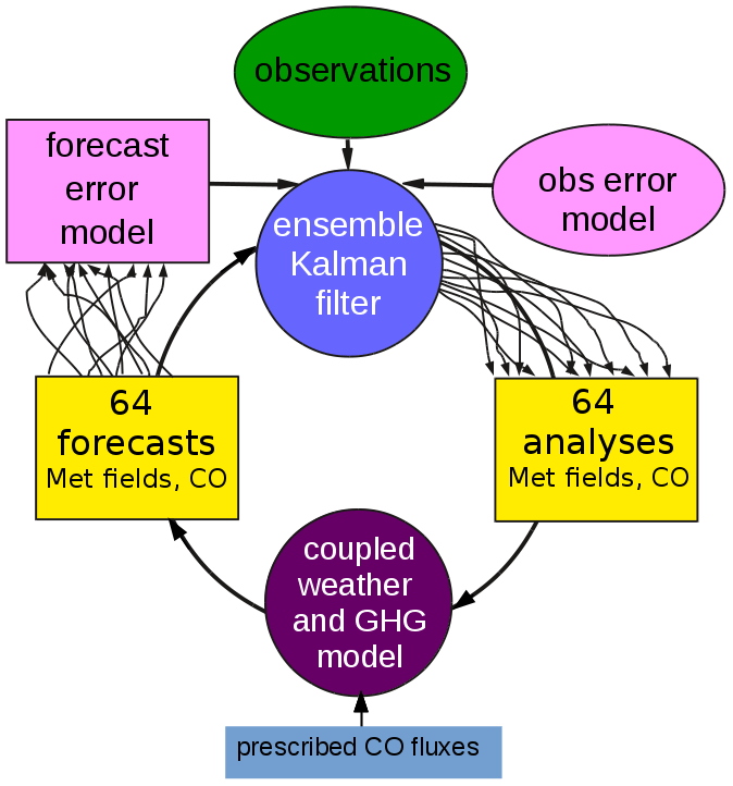
Figure 1 Schematic overview of EC-CAS v1.0. There is an ensemble of 64 prescribed CO surface fluxes. In EC-CAS v1.0, surface flux fields are not estimated; instead, the perturbed flux field is used to account for uncertainty in CO due to error in the surface flux. The 64-member forecast ensemble is used along with the observations, and the statistics of observation errors are used as input for the EnKF. The 64 analyses of meteorology and CO generated by the EnKF are used as initial conditions for the next 6 h forecast. This cycle repeats every 6 h.

The surface flux ensemble (64 members) is generated using a spectral algorithm (see Appendix A of Mitchell and Houtekamer, 2000). The surface flux perturbations are generated such that they are spatially correlated over a distance (half width) of 1000 km. The standard deviation of the spread is set to 40 % of the value of the true surface flux as in Barré et al. (2015). The true surface flux field is used by the 65th ensemble member, which generates the truth trajectory. Two sets of 64 surface flux ensemble members are generated: one for January and February 2015, respectively. Each member of the surface flux ensemble is used with a distinct member of the meteorology ensemble.

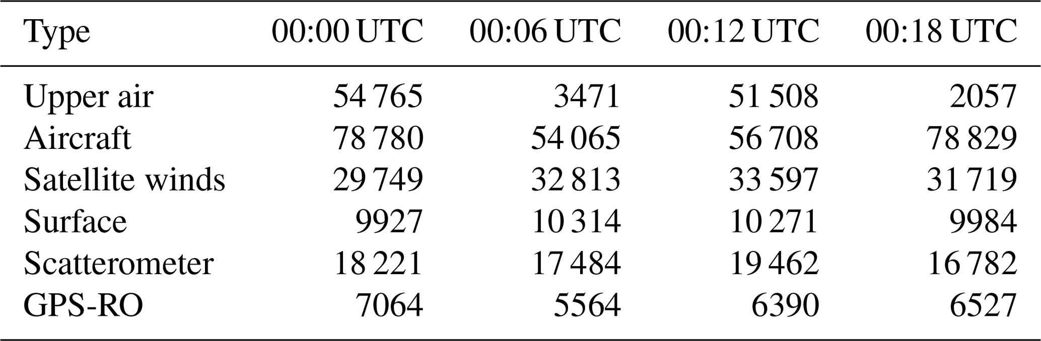
Table 1 Columns shows the typical number of meteorological observations assimilated in each 6 h DA cycle.

Table 2 CO observation networks used in this work.

3.2 Observation networks

The families of meteorological observations used in this work are summarized in Table 1. The location and times of these observations are real, although the observation values are simulated. These meteorological observations are assimilated in all of the experiments presented in this work. The EnKF is tested with five different CO observational networks. These are summarized in Table 2. The first network – HYPNET – is a hypothetical network. It has spatially dense coverage of in situ observations. In this network the observations are located every 1000 km on three planes: 1, 5 and 9 km. These heights are with respect to the local topography. The globally averaged topography is 376 m. Therefore, the heights of these planes with respect to mean sea level are roughly 1.376, 5.376 and 9.376 km. The locations of observations are shown in Fig. 3a.

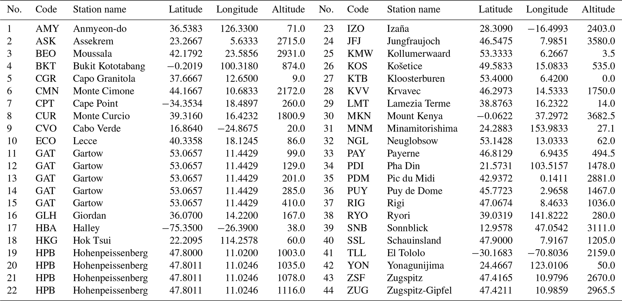
The ECCC surface network (Worthy et al., 2005) consists of 17 observing stations in Canada (see Fig. 3c, d and Table A1). These stations provide measurements at an hourly frequency. Although the ECCC network has expanded rapidly in the past decade to 25 sites in 2020, only the 17 sites providing hourly measurements in 2015 are simulated here. GAW is an acronym of Global Atmospheric Watch (https://gaw.kishou.go.jp, last access: 28 April 2021). The 44 stations from the GAW network used in the current work are shown in Fig. 3c and are listed in Table A2. These stations observe at an hourly frequency. The NOAA surface observation network consists of 69 flasks (see Fig. 3b). The observations from these flasks are temporally sparse, averaging approximately one per week.

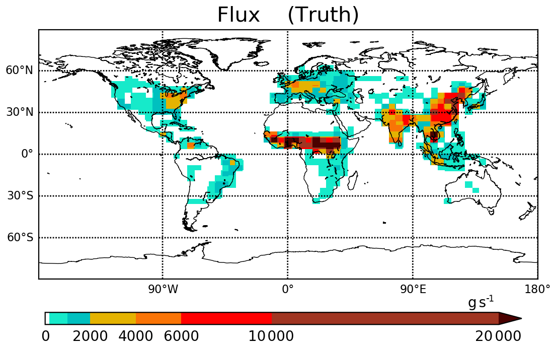
Figure 2 The true CO surface flux field for January 2015.

Figure 3 In each panel, topography is shown using color (see color scale). (a) HYPNET exists at 1, 5 and 9 km. At each of these levels, the observations are located 1000 km apart in the horizontal. There are 622 observation locations at each height and a total of $\mathrm{622}\times \mathrm{3}=\mathrm{1866}$ observations every 6 h. (b) The locations of flask observations from the NOAA network. (c) The GAW and ECCC station locations. (d) The ECCC station locations, which are also shown in the inset of panel (c).

MOPITT (Measurement of Pollution in the Troposphere) (Drummond, 1992) is an instrument onboard the Terra NASA Earth Observation Satellite (EOS) that was launched in December 1999. MOPITT is an important component of the global CO observing system because it measures spectra in both the near-infrared and thermal infrared ranges; thus, its retrieved profiles are sensitive to CO in the lower troposphere during daytime over land, where the flux signal from surface emissions is most readily detected. As a result of this sensitivity to lower tropospheric CO and due to the long observational record, MOPITT data are widely used for inverse modeling of CO emissions and for air quality studies (Arellano and Hess, 2006; Fortems-Cheiney et al., 2011; Barré et al., 2015; Jiang et al., 2015a; Yin et al., 2015; Mizzi et al., 2016; Inness et al., 2019; Gaubert et al., 2020; Miyazaki et al., 2020). It has a nadir footprint of 22 km ×22 km and a 612 km cross-track scanning swath, with an orbit that repeats every 3 d. We used V7J MOPITT data with locations thinned to one observation per grid box. The coverage on a particular day is shown in Fig. 4. The retrieved profiles are reported on a on 10-layer vertical grid, namely surface, 900, 800, … 100 hPa. The MOPITT retrievals y^obs can be described as follows:

$$\begin{array}{}\text{(7)}& {\mathit{y}}^{\mathrm{obs}}={\mathit{y}}^{\mathrm{pr}}+\mathbf{A}({\mathit{x}}^{\mathrm{truth}}-{\mathit{y}}^{\mathrm{pr}}),\end{array}$$

where x^truth is the true atmospheric profile; A is the MOPITT averaging kernel, which reflects the sensitivity of the retrieval to the true state; and y^pr is the a priori profile used in the retrieval. To generate the pseudo MOPITT data, we sample the 65th ensemble model at the locations and times of real MOPITT data, interpolate the profiles to the MOPITT grid, and then apply Eq. (7), with x^truth given by the CO profile from the 65th ensemble member. As a result of the smoothing influence of the retrieval on x^truth, the observations operator for MOPITT must also account for this influence. Consequently, the observation operator is analogous to Eq. (7) and is given by

$$\begin{array}{}\text{(8)}& \mathbf{H}\mathit{x}={\mathit{y}}^{\mathrm{pr}}+\mathbf{A}({\mathit{x}}^{\mathrm{gem}}-{\mathit{y}}^{\mathrm{pr}}),\end{array}$$

where x^gem is the model profile interpolated to the MOPITT vertical grid.

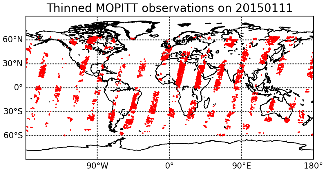
Figure 4 An example of the distribution of MOPITT satellite observations. Thinned MOPITT orbits on 11 January 2015 at 00:00:00 UTC are shown.

In the HYPNET, GAW, ECCC and NOAA networks, the observation operator is an interpolation operator. The HYPNET, GAW, ECCC and NOAA network are temporally static, whereas the MOPITT-like observations change locations depending on the particular DA cycle. The observation errors are set to 10 % of the observation values for all networks in our work. The validation of the MOPITT V7J data by Deeter et al. (2017) found that the standard deviation of the retrieved profiles, relative to independent in situ data varied between 10 % and 16 %. As a result, for the synthetic data generated here, we chose a uniform 10 % observation error.

In summary, five different observation networks are simulated out of which four have a significant impact on the CO estimation error. The idealistic aspects of the design include using simulated (unbiased) observations and ensuring that the truth is consistent with the prior distribution. With these simplifications and a uniformly dense observation network such as HYPNET, we can check that our code is correctly implemented. The estimation errors are obtained from a best-case scenario; therefore, it is expected that higher magnitudes of errors will be obtained with real observations. The benefit of testing EC-CAS with more realistic networks like ECCC, GAW and MOPITT is that it provides a qualitative sense of whether the system is behaving properly, as one can predict how networks with data gaps may behave relative to the uniformly dense network. It should be noted that although the observations are simulated here, we are not performing observing system simulation experiments (OSSEs) (see https://community.wmo.int/wwrp-publications (last access: 28 April 2021) for a discussion of designing OSSEs). OSSEs (Prive et al., 2018) are used to compare the results obtained with different observing systems and require careful configuration and tuning of assimilation system parameters so that conclusions might be quantitatively reasonable.

4 Results

This section discusses the improvement in the CO state due to the assimilation of HYPNET, surface observations and MOPITT-like retrievals, in four separate experiments. The four CO data assimilation experiments are denoted by EXP_HYP, EXP_GAW, EXP_NOAA and EXP_MOP. The EXP_GAW experiment assimilates the GAW and ECCC surface observations, whereas the EXP_NOAA experiment assimilates the NOAA and ECCC surface observations. The improvement is defined with respect to a control experiment, which is referred to as EXP_CNTRL. The control experiment (EXP_CNTRL) assimilates simulated meteorological observations (see Table 1) but does not assimilate simulated CO observations. The CO data assimilation experiments assimilate the same meteorological observations as assimilated by the EXP_CNTRL experiment in addition to their CO observations. The results of the EXP_CNTRL experiment are discussed in Sect. 4.1. Section 4.2 illustrates the role of dynamically changing spatial correlations in an EnKF update. The results of the four CO data assimilation experiments are described in Sect. 4.3.

4.1 Control experiment

Before delving into results of the CO data assimilation, it is important to examine the results of assimilating the meteorological variables. CO is advected by the winds; hence, it is critical to ensure that the assimilation of meteorological observations is working well. Figure 5a shows the time series of global mean temperature forecast and analysis root mean square error (RMSE) from 27 December 2014 at 18:00:00 UTC to 28 February 2015 at 00:00:00 UTC from the EXP_CNTRL experiment; see Sect. S2 of the Supplement for mathematical details of the global mean computation. The RMSE is calculated based on the error between the ensemble mean and the truth which is available at every grid point. As observations are assimilated, the RMSE decreases and stabilizes to 0.5 ^∘C in about 7 d. The RMSE of forecasts and analyses of horizontal wind components and moisture stabilize at similar rates to that of temperature (Fig. 5).

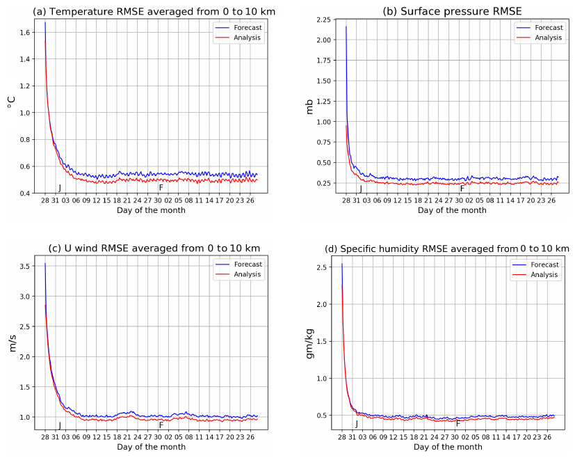
Figure 5 The time series of the RMSE of meteorological variables from the EXP_CNTRL are shown. J and F, marked on the x axis, indicate the start of January and February, respectively. The analyses is shown in red, and the forecast RMSE is shown in blue.

Figure 6 In each panel, column means (0–5 km) averaged from 10 January 2015 at 18:00:00 UTC to 28 February 2015 at 00:00:00 UTC are shown: (a) CO ensemble mean of the control experiment; (b) CO ensemble spread of the control experiment; (c) RMSE of the control experiment; and (d) RMSE of the EXP_HYP experiment.

The column mean of the ensemble mean of CO averaged over the 7-week assimilation period is shown in Fig. 6a. The values of CO are clearly higher in regions of high surface flux (see Fig. 2). The CO from central Africa is advected to the equatorial Atlantic by the easterly winds. Figure 6b shows the ensemble spread of the CO analysis which is estimated by the standard deviation about the analysis mean. This quantifies the expected error from the EnKF in the CO mean. The spread in the CO ensemble at any grid point is due to perturbations in the surface flux and spread in the winds. Figure 6c shows the CO analysis RMSE which quantifies the actual error between the ensemble mean and truth. Clearly, comparing Fig. 6a and c, the RMSE is higher in regions with higher CO values. As noted earlier, the regions with high CO correspond to regions of large surface flux. The similarity of the spatial pattern of the CO ensemble spread (Fig. 6b) and the RMSE (Fig. 6c) and its comparable strength is encouraging because it indicates that the DA system is simulating the actual error well with 64 ensemble members.

The forecast and analysis RMSE are identical because CO observations are not assimilated in the EXP_CNTRL experiment. The time series of RMSE over the analysis period is shown by the blue curve in Fig. 7a. The RMSE in January 2015 stabilizes to about 19 ppb. The surface flux field changes in February 2015 and, hence, the RMSE enters a different regime starting on ∼ 1 February 2015. The RMSE of the control experiment is a baseline against which the RMSE values from CO data assimilations are compared.

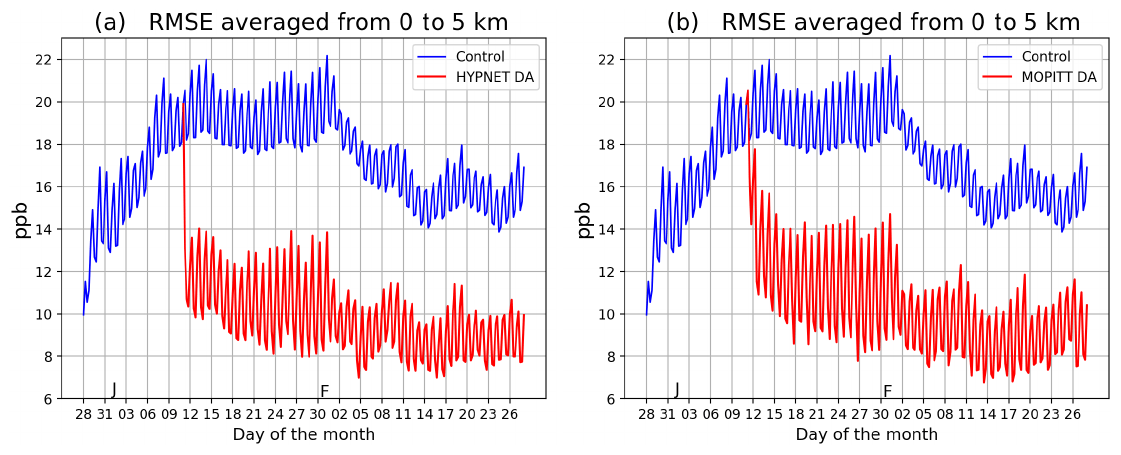
Figure 7 Column (0–5 km) mean RMSE of CO analyses from various experiments: (a) the control, EXP_CNTRL (blue curve), and the DA experiment assimilating HYPNET observations, EXP_HYP (red curve); and (b) the control, EXP_CNTRL (blue curve), and the DA experiment assimilating MOPITT-like observations, EXP_MOP (red curve). The blue curves in panels (a) and (b) are identical. J and F, marked on the x axis, indicate the start of January and February, respectively. The 24 h oscillations in the curves are meteorology induced.

4.2 Role of estimated correlations

The correlations estimated using the forecast ensemble play a key role in spreading the information from a given CO observation to other grid points for any observational network. The correlation estimate changes dynamically depending on the surface flux perturbations and winds. This state dependence of the sample correlation is an important characteristic of ensemble-based filters. The role of the sample correlation and physical localization is illustrated for an observation located at Toronto.

Figure 8 shows the spatial correlation structure for the Toronto location at two different times from EXP_CNTRL. In Eq. (1), the term (y^o(t)−H(t)x^f(t)) is the “innovation”. This quantity is in observational space and is, thus, a scalar for the case of a single observation located in Toronto. The sample correlation P^f(t)H^T(t) is used to map the innovation into model space. This is the correlation between the ensemble of x^f(t) and H(t)x^f(t). For simplicity, we take the nearest grid point to Toronto as its actual location so that H(t) is a row vector of zeros with one at the index corresponding to the Toronto grid point. The innovation in CO at the Toronto grid point updates the CO at all the other grid points in proportion to the correlation as estimated by the forecast ensemble. The regions of high correlation change significantly from 15 January 2015 at 06:00:00 UTC to 22 January 2015 at 12:00:00 UTC. Consequently, the impact of the CO observation at Toronto on other grid points is different on 15 January 2015 at 06:00:00 UTC and 22 January 2015 at 12:00:00 UTC. In theory (that is, given an infinite ensemble size), a given CO observation should update the CO estimate at all other grid points globally. However, with a small ensemble size, spurious correlations develop and, hence, physical localization is required so that a given CO observation updates the CO state only within a limited region defined by the horizontal localization radius (hlr) and vertical localization radius (vlr) (see Sect. 2.4). The red circle in Fig. 8 has radius of hlr =2000 km. The Gaspari–Cohn function (Houtekamer and Mitchell, 1998) used for physical localization has its maximum in Toronto and decays moving away from the observation's location. This function is used as a weight to modulate the correlation values. As a result, the impact of the observation decays with distance from the observation. Distance-dependent localization assumes that the sample correlation given by the ensemble is less trustworthy (more likely to be spurious) as one moves further away from the observation. As noted in Sect. 2.4, variable localization ensures that CO observations do not update meteorological variables. Therefore, the estimates of meteorological variables are the same in all of the experiments.

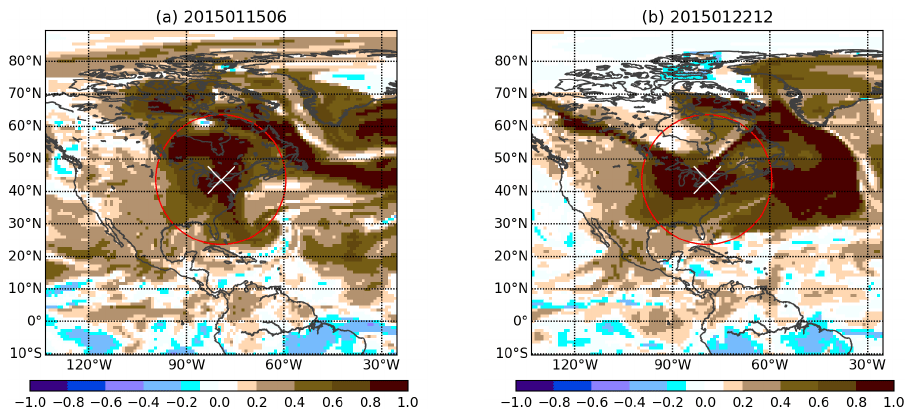
Figure 8 The spatial correlation of CO between Toronto (shown by the white cross) and other locations in the horizontal plane defined by the lowest model level. The red circle – representing a 2000 km radius – shows the horizontal localization. The correlation is estimated using the 64 forecast ensemble members.

4.3 CO DA experiments

The EXP_HYP experiment assimilates HYPNET observations (see Sect. 3.2) in addition to the same meteorological observations assimilated in the EXP_CNTRL experiment. The HYPNET observations are assimilated starting on 10 January 2015 at 18:00:00 UTC after a spin-up from 27 December 2014 at 18:00:00 UTC to 10 January 2015 at 18:00:00 UTC. This spin-up period allows time for the meteorological assimilation to stabilize (Fig. 5) before the CO data assimilation begins. This spin-up also helps the development of correlations within the CO field.

Figure 6d shows the column-averaged CO RMSE for the EXP_HYP experiment. Compared with the RMSE for the EXP_CNTRL experiment, the RMSE decreases substantially because HYPNET observations effectively constrain the CO state. The time series of RMSE for the EXP_HYP experiment is shown by the red curve in Fig. 7a. The blue and red curves overlap from 27 December 2014 at 18:00:00 UTC to 10 January 2015 at 18:00:00 UTC during the spin-up period. As soon as CO observations are assimilated starting on 10 January 2015 at 18:00:00 UTC, the RMSE decreases. The reduction in the RMSE due to the assimilation of HYPNET observations is ∼7 ppb. This reduction is defined as the “benefit”:

$$\begin{array}{}\text{(9)}& \mathrm{benefit}=\mathrm{RMSE}\left(\mathrm{control}\right)-\mathrm{RMSE}\left(\mathrm{DA}\right).\end{array}$$

The relative benefit is defined as

$$\begin{array}{}\text{(10)}& \mathrm{relative}\mathrm{\_}\mathrm{benefit}=\mathrm{100}\times {\displaystyle \frac{\mathrm{benefit}}{\mathrm{RMSE}\left(\mathrm{control}\right)}}.\end{array}$$

The second term in Eq. (9) is the RMSE of the experiment which assimilates CO observations. As the EXP_CNTRL experiment does not assimilate CO observations, the benefit measures the value of assimilating CO observations from a particular network. This metric quantifies the extent to which CO observations constrain the CO state. Figure 9a shows the spatial structure of the benefit in the EXP_HYP experiment. This figure is basically the difference between Fig. 6c and d. The benefit is positive in most parts of the globe except in parts of Tibet and eastern China. A negative benefit value means that the assimilation of CO observations increased the RMSE compared with the EXP_CNTRL experiment. Negative values can occur because of the statistical nature of data assimilation. However, if the data assimilation system is well tuned, such regions of negative benefits should be few and small, as seen here. By comparing the spatial structure of the RMSE in Fig. 6c and the benefit in Fig. 9a, it is clear that the benefit is proportional to the RMSE. This makes sense because where the RMSE is large, the observations have a larger scope for improving the CO state estimate. The mean relative benefit (Eq. 10) in this experiment is 41 %. This means that the assimilation of HYPNET observations decreases the control RMSE by 41 %.

Figure 9 Column (0–5 km) mean benefit averaged from 10 January 2015 at 18:00:00 UTC to 28 February 2015 at 00:00:00 UTC. In panel (a), the marked boxes show the domains of North America, South America, Europe, Africa, South Asia and East Asia. These domains are used in Fig. 11. Note that all of the domains contain both ocean and land. The South American domain includes a large part of the Pacific Ocean.

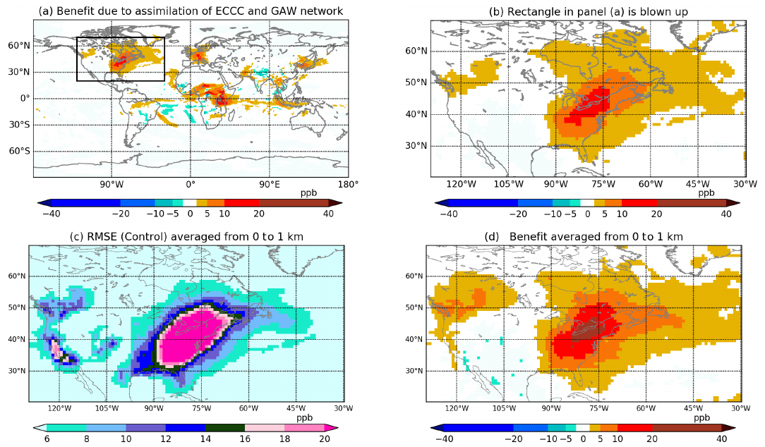
Figure 10 In all panels, the averages from 10 January 2015 at 18:00:00 UTC to 28 February 2015 at 00:00:00 UTC are shown: (a) column (0–5 km) mean benefit from EXP_GAW; (b) the North American domain from panel (a); (c) column (0–1 km) mean RMSE from EXP_CNTRL; and (d) column (0–1 km) mean benefit from EXP_GAW.

The time series of the RMSE from the EXP_MOP experiment is shown by the red curve in Fig. 7b. The similarity of the amplitudes (about 9 ppb) of the red curves in Fig. 7a and b indicates, surprisingly, that the global benefit of MOPITT-like data is only a little worse than that due to the hypothetically dense in situ network (HYPNET). However, in our experiments, the observations are unbiased and the observation operator is perfect. The spatial structure of the benefit due to the assimilation of MOPITT-like retrievals (EXP_MOP) is shown in Fig. 9b. By comparing Fig. 9a and b, it is evident that the benefit due to the assimilation of HYPNET observations and MOPITT-like retrievals is also comparable in the column mean, in spite of the different spatiotemporal distribution of observations. The mean relative benefit due to the assimilation of MOPITT-like retrievals is 38 % whereas that due to assimilation of HYPNET is 41 %.

Figure 10a shows the benefit of the EXP_GAW experiment. Both the GAW and ECCC networks are assimilated in this experiment. The combined network is temporally dense with observations every hour but is spatially sparse except in Canada and western Europe (Fig. 3c, d). The relative benefit in this experiment is 8 %. Figure 10b shows the benefit over North America averaged from 0 to 5 km. All of the ECCC stations are located in the bottom 1 km. Figure 10d shows the benefit over North America averaged from 0 to 1 km. The bulk of the benefit is in the eastern part of this domain, although the ECCC stations are located both in eastern and western Canada. The area of highest benefit of about 10–40 ppb is centered on ECCC stations located in Ontario. Even though no stations are located in the USA in this experiment, the benefit of observations in Ontario reaches as far as Florida, spreading throughout eastern USA. This is because of the flow-dependent spatial correlation between locations of observations in Ontario and the eastern part of USA, which is evident in Fig. 8, as well as subsequent downstream transport during the forecast step. The western part of Canada has a weak benefit in spite of having several observation sites in this region. This is because the RMSE in the western region is substantially lower than that in the eastern region (see Fig. 10c). Thus, there is little scope for the observations to improve upon the control RMSE. The relative benefit over North America is 38 %.

Figure 10a shows that the assimilation of GAW observations results in significant benefit over Europe and parts of central Africa. The benefit in Europe is due to the high spatial density of GAW stations there. However, with only five stations in Africa, a benefit of 5–20 ppb in central Africa is produced. Some benefit is also seen over northeastern China and Malaysia due to GAW stations located in these regions.

The last experiment, EXP_NOAA, assimilates data from the NOAA flask stations in addition to those from the ECCC surface stations. It is seen (figure not shown) that the benefit over Canada is the same as that seen in EXP_GAW. However, globally, the NOAA flask stations do not result in any significant benefit over any other region. This is because the flask observations are available, on average, only once a week. This experiment is not discussed further in this work.

Figure 11 Profiles of the benefit and control RMSE averaged over different domains. In each panel, the black curve shows the control RMSE scaled down by a factor of 3. The colored curves show the benefits due to the assimilation of three different observational networks (EXP_HYP, EXP_MOP and EXP_GAW). Panel (a) shows the globally averaged profiles. The other panels show profiles averaged over the domains shown in Fig. 9a. The limits on the x axis are different in each panel.

In the case of the assimilation of HYPNET and MOPITT-like observations (Fig. 9a, b), many parts of the Atlantic, Pacific, Indian and other oceans show significant benefit. The CO surface flux over oceans is practically zero compared with that on land. The HYPNET and MOPITT-like observations over oceans contribute to the benefit over oceans. However, the improvement of the CO state over land also contributes to the benefit over oceans. For example, any improvement in the CO state over central Africa improves the state over tropical Atlantic ocean due to the downwind transport.

In the discussion so far, the horizontal and temporal structure of benefit was explored. Figure 11 examines the vertical structure of benefit. Figure 11a shows the globally averaged profile of the control RMSE and benefits from the three CO DA experiments. The average RMSE of the control experiment (EXP_CNTRL) peaks close to the surface with a value of 21 ppb. The average benefit in the bottom 4 km is ∼7 ppb in the EXP_HYP and EXP_MOP experiments. Comparing the shapes of the blue and red curve to the black curve, the benefit is proportional to the control RMSE except in the bottom ∼1 km. The shape of the benefit profile is dictated both by the shape of the control RMSE and the location of observations in the particular network. The EXP_HYP profile shows a local peak at 1 km. This is because HYPNET observations are located at 1 km. HYPNET observations are also located at 5 km. However, the control RMSE decreases by a factor of 2 from 1 to 5 km; consequently, the benefit also decreases. The peak in the blue profile at ∼3 km is due to a combination of RMSE values and information content in the MOPITT-like retrievals.

The profiles averaged over Africa (Fig. 11b) have similar shapes to those in Fig. 11a. This is because both the RMSE and benefit in Africa are high compared with other parts of the globe (see Figs. 6c and 9). Hence, the global average is dominated by values over Africa. The average height of the GAW observations is 2.2 km. The benefit in the EXP_GAW experiment has a peak value of ∼4 ppb at 3.5 km. This is because the GAW station located at Mount Kenya (0.06^∘ S, 37.29^∘ E) has an altitude of 3678 m. Additionally the site at Assekrem, Algeria (23.26^∘ N, 5.63^∘ E), is situated at an altitude of 2715 m. The EnKF spreads the information content from these observations to the surrounding regions through the flow-dependent covariances used in the analysis step and through downstream transport in the forecast step.

The profiles for North America are shown in Fig. 11c. The average height of the ECCC observations is 0.38 km. The benefit due to the ECCC observations close to the surface is ∼4.1 ppb. The benefit due to the assimilation of ECCC observations decreases monotonically with height because the RMSE decreases monotonically and also because the ECCC observations cannot constrain the CO state beyond the vertical localization radius. The average height of stations in eastern Canada is 0.212 km. These stations make a major contribution to the benefit over North America. Temporally HYPNET observes every 6 h, whereas ECCC stations observe every hour. Both the higher temporal frequency and the lower altitude contribute to the higher benefit close to the surface in case of the ECCC observations compared with HYPNET observations, which are located at about 1 km.

Figure 11d shows the profiles for Europe. The average height of the GAW observations is 1.13 km. In the case of the GAW network, the benefit is 5.9 ppb close to the surface. As in the case of North America, the better performance of GAW stations in the bottom 500 m is a due to both the lower altitude of the stations and the higher temporal frequency of observations compared with the HYPNET.

It is evident that the spatiotemporal structure of the benefit is similar between HYPNET and MOPITT, both horizontally and vertically. This suggests that, in the idealistic setting of unbiased observations and precisely known observation and model error covariances, the performance of MOPITT-like retrievals is similar to in situ observations. It should be noted that MOPITT-like observations are spatially more dense than our HYPNET observation network. HYPNET has information at three vertical levels, whereas MOPITT has an information content with 1 or 2 degrees of freedom (Deeter et al., 2012) so that limited vertical information is provided by the two networks.

5 Conclusions and further work

A new atmospheric composition data assimilation system based on an operational weather forecast model (EC-CAS v1.0) was developed and validated for the estimation of the three-dimensional state of CO using simulated observations from the HYPNET, ECCC, GAW and MOPITT networks. The spread in CO is obtained by perturbing the winds, surface flux fields and physics parameterizations. The CO spread approximately matches the RMSE, suggesting that an ensemble size of 64 is acceptable for CO estimation. However, these conclusions are based on the assimilation of simulated observations which are unbiased.

These experiments lead to a qualitative understanding of the decrease in RMSE due to the assimilation of observed CO from realistic networks. With all of the networks, it is seen that the benefit due to the assimilation of CO observations is proportional to the CO RMSE. Another factor that controls the pattern of the benefit is the location of observations; for example, the GAW network has only one station in central Africa, and the observations from this station are able to effectively constrain the CO state within 2000 km, which is the localization radius used in these experiments. The benefit is the highest in the plane at which this observation is located. The CO state close to the surface is better constrained by observations in the lowermost 500 m than observations at 1 km. This is suggested by the results in North America and Europe. The CO state over the ocean is constrained due to the improvement of the CO state over surface-flux-rich land regions which is transported downstream during the forecast and also due to the assimilation of observations over the oceans. In the case of MOPITT-like data assimilation, the benefit in central Africa (which is the region with the strongest surface flux) ranges from 10 to over 40 ppb. The downwind transport results in a benefit of 5 to 40 ppb over the tropical Atlantic. The benefits over southern and eastern Asia range from 2 to 20 ppb. These quantitative findings are expected to change when real observations are assimilated. Biases in observations and correlations in the observational errors along with model errors that are unaccounted for make the assimilation of real observations more challenging; thus, the error reductions are expected to be smaller.

This work has presented only the very first step in the development of EC-CAS. There are many further stages of development because the goal of EC-CAS is to estimate the three-dimensional fields of CO, CO₂ and CH₄ and their surface fluxes along with meteorological fields by assimilating all available observations of meteorological variables and chemical species using an ensemble smoother. These include both in situ and remotely sensed measurements. The immediate next step is to modify EC-CAS 1.0 to allow the update of the CO surface flux by CO observations, as we demonstrated here that the CO state estimation is working well. After the ability to estimate surface fluxes is demonstrated, EC-CAS will be tested for the estimation of CO and CO₂ three-dimensional fields and their surface fluxes using real observations. The estimates of surface flux can be improved using a smoother (Liebelt, 1967) rather than a filter, as a smoother assimilates observations earlier as well as later than the analysis time. Ultimately, an ensemble Kalman smoother (Bocquet, 2016) will be developed.

Appendix A

Table A1 Information about ECCC surface sites used in this study. The altitude is given in meters above sea level.

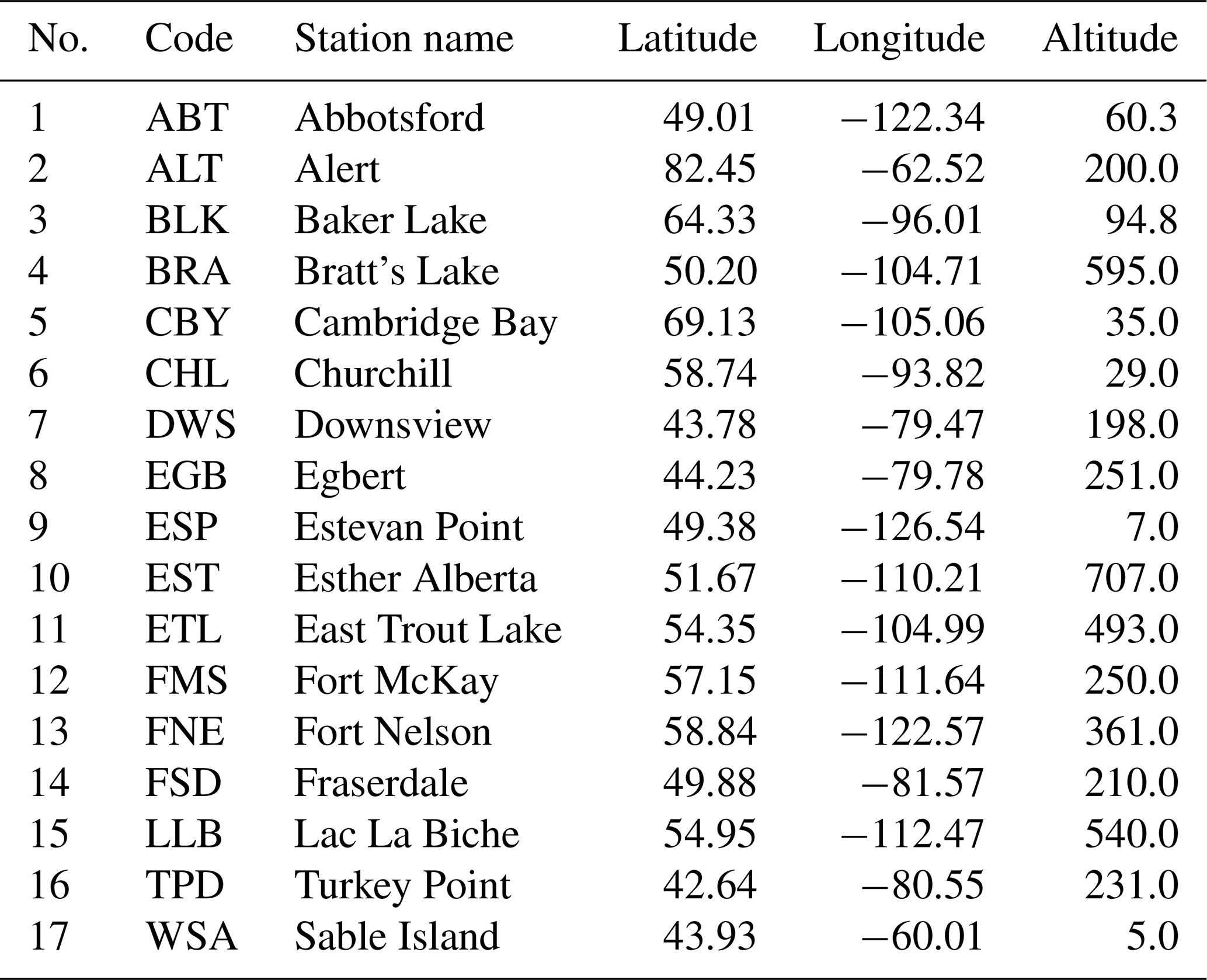
Table A2 Information about GAW surface sites used in this study. The altitude is given in meters above sea level.