the Creative Commons Attribution 4.0 License.
the Creative Commons Attribution 4.0 License.
 | 03 May 2021
pyPI (v1.3): Tropical Cyclone Potential Intensity Calculations in Python
Daniel M. Gilford
Potential intensity (PI) is the maximum speed limit of a tropical cyclone found by modeling the storm as a thermal heat engine. Because there are significant correlations between PI and actual storm wind speeds, PI is a useful diagnostic for evaluating or predicting tropical cyclone intensity climatology and variability. Previous studies have calculated PI given a set of atmospheric and oceanographic conditions, but although a PI algorithm – originally developed by Kerry Emanuel – is in widespread use, it remains under-documented. The Tropical Cyclone Potential Intensity Calculations in Python (pyPI, v1.3) package develops the PI algorithm in Python and for the first time details the full background and algorithm (line by line) used to compute tropical cyclone potential intensity constrained by thermodynamics. The pyPI package (1) provides a freely available, flexible, validated Python PI algorithm, (2) carefully documents the PI algorithm and its Python implementation, and (3) demonstrates and encourages the use of PI theory in tropical cyclone analyses. Validation shows pyPI output is nearly identical to the previous potential intensity computation but is an improvement on the algorithm's consistency and handling of missing data. Example calculations with reanalyses data demonstrate pyPI's usefulness in climatological and meteorological research. Planned future improvements will improve on pyPI's assumptions, flexibility, and range of applications and tropical cyclone thermodynamic calculations.
- Article
(5675 KB) - Full-text XML
- BibTeX
- EndNote


Tropical cyclones pose significant risks to coastal societies, being among the costliest and deadliest of global natural hazards (e.g., Pielke et al., 2008; Rappaport, 2014; Hsiang and Jina, 2014). Damages increase exponentially with tropical cyclone intensity (∼5 % per m s−1; Murnane and Elsner, 2012), so it is crucial to understand and accurately bound tropical cyclone maximum wind speeds. Theoretical and numerical models (e.g., Emanuel, 1987; Tsuboki et al., 2015; Sobel et al., 2016; Wehner et al., 2018) along with recent observations (Kossin et al., 2020) indicate that climate change has already increased storm intensities – a trend expected to continue as the Earth system warms. Emanuel (2005) showed the total destructive potential of tropical cyclones (derived from time-integrated maximum intensity) has increased since the 1970s. Elsner et al. (2008) showed that the most intense observed tropical cyclones are getting stronger, and a more recent comprehensive study shows that the number of major (Category 3+) tropical cyclones has increased over the past 40 years (Kossin et al., 2020). Given the links between intensity and tropical cyclone impacts, it is worthwhile to develop and improve modeling tools for diagnosing and predicting tropical cyclone intensities.
Potential intensity (PI) is a theoretical model for the upper bound (colloquially known as the “speed limit”) on tropical cyclone intensity, given environmental conditions and energetic constraints (e.g., Emanuel, 1986; Holland, 1997). PI has several properties which make it a particularly useful model for studying tropical cyclones. First, PI is statistically linked to the lifetime maximum intensities of observed storms (Emanuel, 2000), so it can be used to assess and interpret real-world intensity trends and variability (e.g., Wing et al., 2007; Gilford et al., 2019; Shields et al., 2019). Second, PI can be readily calculated from standard atmospheric profiles (either modeled or observed), making it flexible across many applications and spatiotemporal scales. Third, PI may be decomposed into thermodynamic and parametric contributions that enable budget and sensitivity analyses – with direct implications for real-world storms. Finally, as a theoretical model grounded in meteorological data, it is well-suited for incorporation into prognostic and diagnostic indices of intensification (e.g., the ventilation index, VI; Tang and Emanuel, 2012), tropical cyclogenesis (e.g., VI; the genesis potential index, GPI; Camargo et al., 2007; the tropical cyclone genesis index, TCGI; Tippett et al., 2011), and destructive potential (e.g., the power dissipation index, PDI; Emanuel, 2005).
The algorithm to compute PI was originally developed by Bister and Emanuel (2002) (hereafter BE02), coded as a FORTRAN subroutine. It was later converted for use as a MATLAB function by Kerry Emanuel and has been irregularly revised by Kerry Emanuel and other collaborators/colleagues. The BE02 PI function has been extensively (and nearly universally) used and/or adapted by the tropical meteorology community to calculate PI for modeling, observational, and theoretical research applications (e.g., McTaggart-Cowan et al., 2008; Gualdi et al., 2008; Camargo et al., 2009; Sobel and Camargo, 2011; Tippett et al., 2011; Bryan, 2012; Vecchi et al., 2013; Ramsay, 2013; Camargo, 2013; Chavas and Emanuel, 2014; Strazzo et al., 2016, 2015; Wing et al., 2015; Sobel et al., 2016; Polvani et al., 2016; Lin and Emanuel, 2016; Gilford et al., 2017; Xu et al., 2019; Gilford et al., 2019; Emanuel, 2018; Shields et al., 2019; Camargo and Polvani, 2019, and many others). The BE02 function is also used to compute daily maps of North Atlantic PI for meteorological assessment in real time (produced by the Center for Land–Atmosphere Prediction1; Emanuel et al., 2004).
Despite widespread use, the BE02 algorithm itself has never (to my knowledge) been fully documented. Because it is an important modeling tool for tropical cyclone intensity, there is a need for a transparent and documented PI algorithm. It is also advantageous to implement a PI algorithm in Python (which is freely available and has many advantages in scientific research; Millman and Aivazis, 2011), to complement the existing counterparts in MATLAB (which is proprietary and therefore less accessible) and FORTRAN (which is not easily extensible for a broad range of applications; Rashed and Ahsan, 2018).
I developed Tropical Cyclone Potential Intensity Calculations in Python (i.e., “pyPI”) to meet these needs. In addition to adapting the BE02 algorithm in Python and thoroughly documenting the model, pyPI provides a maintained and regularly archived repository to support open science in the tropical meteorological community. pyPI is also ideally suited for ongoing community development and improvement and for research applications which require flexibility in particular PI input parameters or components (for example, the computation of the lifting condensation level) or integration with other Python packages. This article provides context for the initial package release of pyPI (v1.3) and details its development, algorithm, validation, and sample applications.
The proceeding Sect. 2 provides a brief overview of potential intensity theory and introduces its key components including thermodynamic efficiency and disequilibrium. Section 3 presents the mathematical basis of pyPI's potential intensity computations. We describe the Python implementation of the pyPI algorithm in Sect. 4, including its adjustable input parameters and handling of missing data. Model validation in Sect. 5 demonstrates that pyPI output is nearly identical to the previously published MATLAB algorithm, with minor improvements for consistency. Section 6 illustrates several climatological applications of pyPI. The study concludes with a discussion of planned pyPI advancements in Sect. 7.
Tropical cyclones arise as an indirect response to a thermodynamic gap in the tropical atmosphere's energy budget (e.g., Emanuel, 2006). The tropical surface's output longwave radiative cooling is outpaced by combined solar and longwave radiative heating (terrestrially sourced by greenhouse gases and clouds) received at the surface. In the absence of any balancing outgoing process, the resulting thermodynamic disequilibrium would lead to a buildup of heat driving substantially higher surface temperatures (e.g., Manabe and Strickler, 1964). Instead, atmospheric convection plays the leading role in removing this excess heat; tropical cyclones are a well-known expression of this convection.
Driven by thermodynamic disequilibrium – which is largest in the summer and autumn seasons – an existing mature tropical cycle will transfer heat from the surface to the atmospheric boundary layer, largely through latent heat release of evaporation and from the sea surface and dissipative heating (Bister and Emanuel, 1998). Viewed from this perspective, it is useful and convenient to model tropical cyclones as Carnot heat engines (Emanuel, 1987) which convert this fuel (i.e., thermodynamic disequilibrium) to kinetic energy in the form of azimuthal winds. Figure 1 shows a diagram of a Carnot cycle overlaid on a cross section of a mature tropical cyclone, along with the pyPI algorithm inputs and outputs.
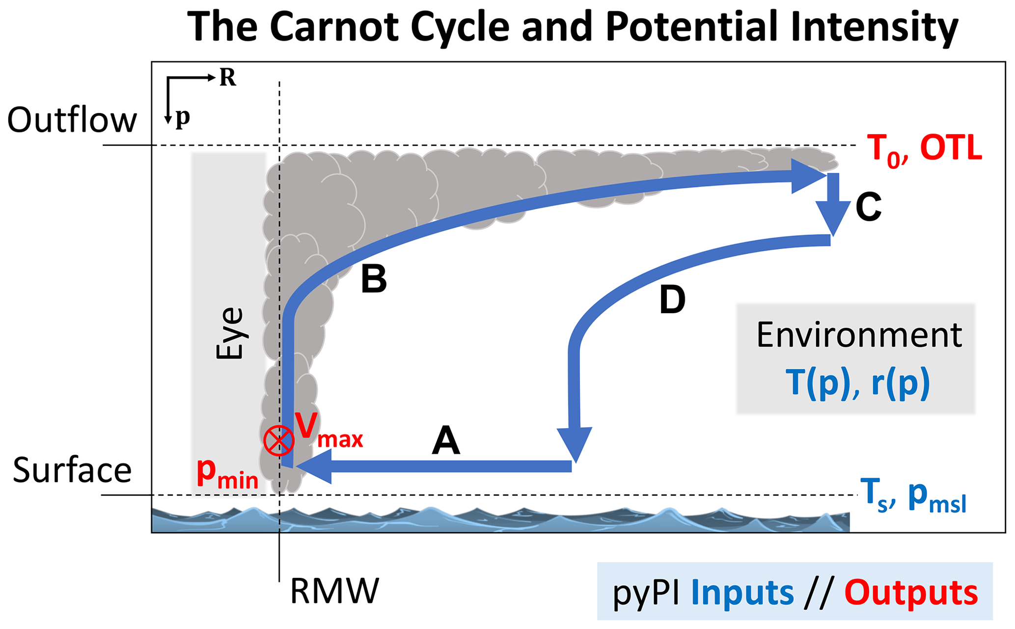
Figure 1The cross section (along radius, R, and pressure, p) of an idealized and mature tropical cyclone and its thermodynamic cycle. pyPI inputs and outputs are in blue and red text, respectively, and are defined in Table 1. Bold blue lines and black letters indicate the four branches of the Carnot cycle, A through D (see text). The tropical cyclone maximum potential intensity (Vmax) is found at the radius of maximum winds (RMW) and is directed into the page in the Northern Hemisphere. The minimum central pressure (pmin) is found in the storm's eye. Based on Carnot cycle illustrations in Emanuel (1987, 2006).
Following the entropy gradient, air at the outer reaches of the storm spirals inward (branch A) toward the minimum central pressure in the eye (pmin) and the entropy maximum near the radius of maximum winds (RMW). Along its motion this air gathers entropy through isothermal heat absorption (through the two processes noted above) with the temperature of the sea surface, Ts. When the air reaches an entropy maximum at the RMW it bends upward through adiabatic expansion (branch B), conserving its entropy as it rises through the eyewall and then along the outflow at the storm top. This outflow layer is called the “outflow temperature level” (OTL), and here the air undergoes isothermal radiative heat loss (branch C) with temperature T0, transferring the entropy generated by the storm to its surroundings. Finally, the Carnot cycle closes as the air undergoes adiabatic compression with lower entropy back towards the sea surface (branch D) while its temperature rises once again.
An advantage of this theoretical model of a tropical cyclone is that it permits a formulation of the storm's theoretical maximum intensity – i.e., its PI – in terms of the heat engine efficiency, defined by the temperatures at each extent (reservoir) of the engine (), and in terms of the heat source itself (i.e., thermodynamic disequilibrium). These quantities may be estimated with atmospheric and oceanic observations (Sect. 5.1).
As derived in Bister and Emanuel (1998) and Emanuel (2003), the maximum (near-surface) potential intensity of a tropical cyclone, Vmax, may be approximated by
where Ck and CD are the enthalpy and momentum surface exchange coefficients, respectively, is the saturation moist static energy at the sea surface, and h* is the saturation moist static energy of the air above the boundary layer (often evaluated at ∼500–600 hPa; cf. Wing et al., 2015). Tropical cyclone thermodynamic disequilibrium and efficiency are represented by the terms and , respectively; the ratio is a defined constant that may be estimated from theory or observations (Sect. 4.1).
In physically based axisymmetric models, mature tropical cyclone wind speeds tend to reach their PI (e.g., Rotunno and Emanuel, 1987). In contrast, observed storms rarely attain their thermodynamically constrained potential intensities (see limitations discussed in Sect. 7). However, Emanuel (2000) combined climatologically derived PI with observed tracks and intensities of real-world storms to show that any observed storm statistically has an equal likelihood of attaining any lifetime maximum speed between some lower bound and the PI along its track. This is a powerful statistical property, because it implies that any shift in the PI distribution – either on short timescales such as during an anomalously cold summer or on long timescales such as a response to a warming climate – will be accompanied by similar shifts in the observed intensity distribution (cf. Wing et al., 2007). Gilford et al. (2019) showed that randomly sampled observed intensity distributions which have at least 25 tropical cyclones (of hurricane strength or greater) will robustly follow their associated along-track potential intensity distributions.
Links between observed and potential intensities have been shown on seasonal (Tonkin et al., 2000; Gilford et al., 2019), interannual (Wing et al., 2007; Shields et al., 2019), and climatological (e.g., Emanuel, 2000) timescales. The relationship is more robust when PI is evaluated along the track of a storm rather than as a basin-wide average (Wing et al., 2007; Gilford et al., 2019; Shields et al., 2019). Other studies have examined the roles of volcanic eruptions/lower stratospheric variability (e.g., Emanuel et al., 2013), the Montreal Protocol (Polvani et al., 2016), or climate change on potential intensity (Emanuel, 2005; Vecchi et al., 2014; Sobel et al., 2016). Any oceanic or atmospheric variability or trend which alters the thermodynamic environments of tropical cyclones could have some effect on PI (though the relative importance and/or statistical significance of these effects will vary). The connection between tropical cyclone PI and climate change will likely remain a critical topic to understand: the troposphere continues to warm and moisten in response to anthropogenic emissions of greenhouse gases while simultaneously the lower stratosphere is cooling (e.g., IPCC, 2013; Santer et al., 2013).
3.1 BE02 PI formulation
This section provides a detailed description and record (including relevant citations) of the PI algorithm with its thermodynamic/meteorological origins, assumptions, and computations.
Potential intensity may be derived following Bister and Emanuel (2002) (which is largely based on the formulation of Emanuel, 1995) idealizing a tropical cyclone as a Carnot heat engine (e.g., Emanuel, 1987) and assuming the following: (1) the work done against friction by the outflow is ignored, (2) when the storm intensity reaches its maximum, the anticyclone at the top of the storm is fully developed, and (3) the gradient wind may be approximated by cyclostrophic wind at the RMW. Under these conditions, the Carnot cycle formulation yields an expression for the maximum potential intensity (which roughly scales with the approximated PI expression, Eq. 1; Wing et al., 2015):
where CAPE* is the convective available potential energy of saturated air lifted from sea level to the outflow level referencing the environmental profile, and CAPEenv is the convective available potential energy of the environment. Because the final term is evaluated at the RMW and CAPE* is pressure dependant, an expression for the surface pressure at the RMW is needed. Following Bister and Emanuel (2002) (cf. also Garner, 2015, their Eq. 6), the minimum pressure of the tropical cyclone at the RMW, pm, is found with2
where Tυ is the surface environmental virtual temperature, and CAPE|RMW is the environmental convective available potential energy evaluated at the RMW. Because the boundary layer water vapor mixing ratio is higher in the tropical cyclone eyewall than the storm's outer region (assuming a constant relative humidity in the boundary layer across the storm's radius), CAPE|RMW is slightly larger than CAPEenv (discussed more below).
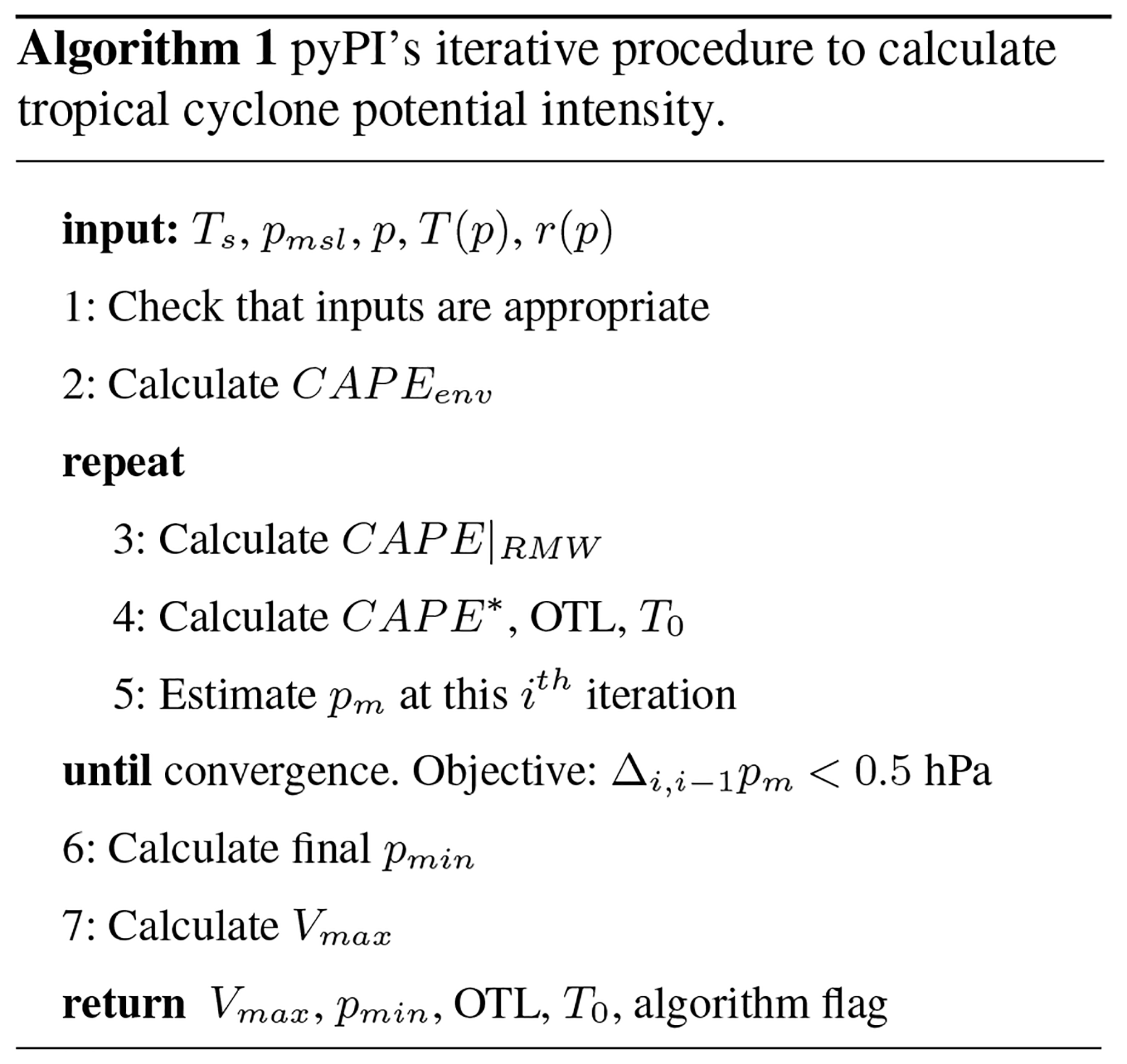
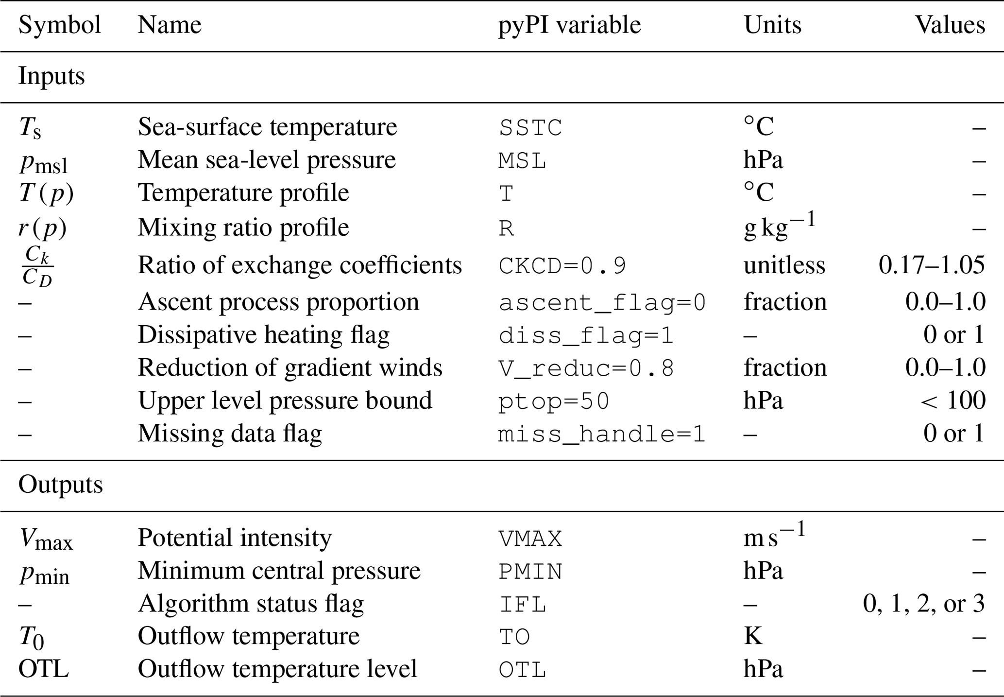
Table 1Input and output variables and adjustable algorithm parameters for the PI module. Default parameter values are specified in the “pyPI variable” column. Parameters adjusted by the user should never be set outside the “Values” column prescriptions without physical justification and/or appropriate module modification.
The pressure dependence of CAPE requires solving Eqs. (2) and (3) with numerical iteration, which pyPI performs with individual PI and CAPE modules. Algorithm 1 summarizes how pyPI computes maximum potential intensity by modeling a tropical cyclone as a Carnot heat engine. Algorithm inputs and outputs are provided in Table 1 and described in Sect. 4; meteorological constants are provided in the Appendix (Table A1). We begin by describing the CAPE calculation, which is used throughout the pyPI algorithm.
3.2 CAPE module
CAPE is defined as the sum of positive and negative areas of buoyancy energy of a lifted parcel on a sounding (e.g., Emanuel, 1994, their Eq. 6.3.6, discussed more below) and is calculated by pyPI with the procedure in Algorithm 2.
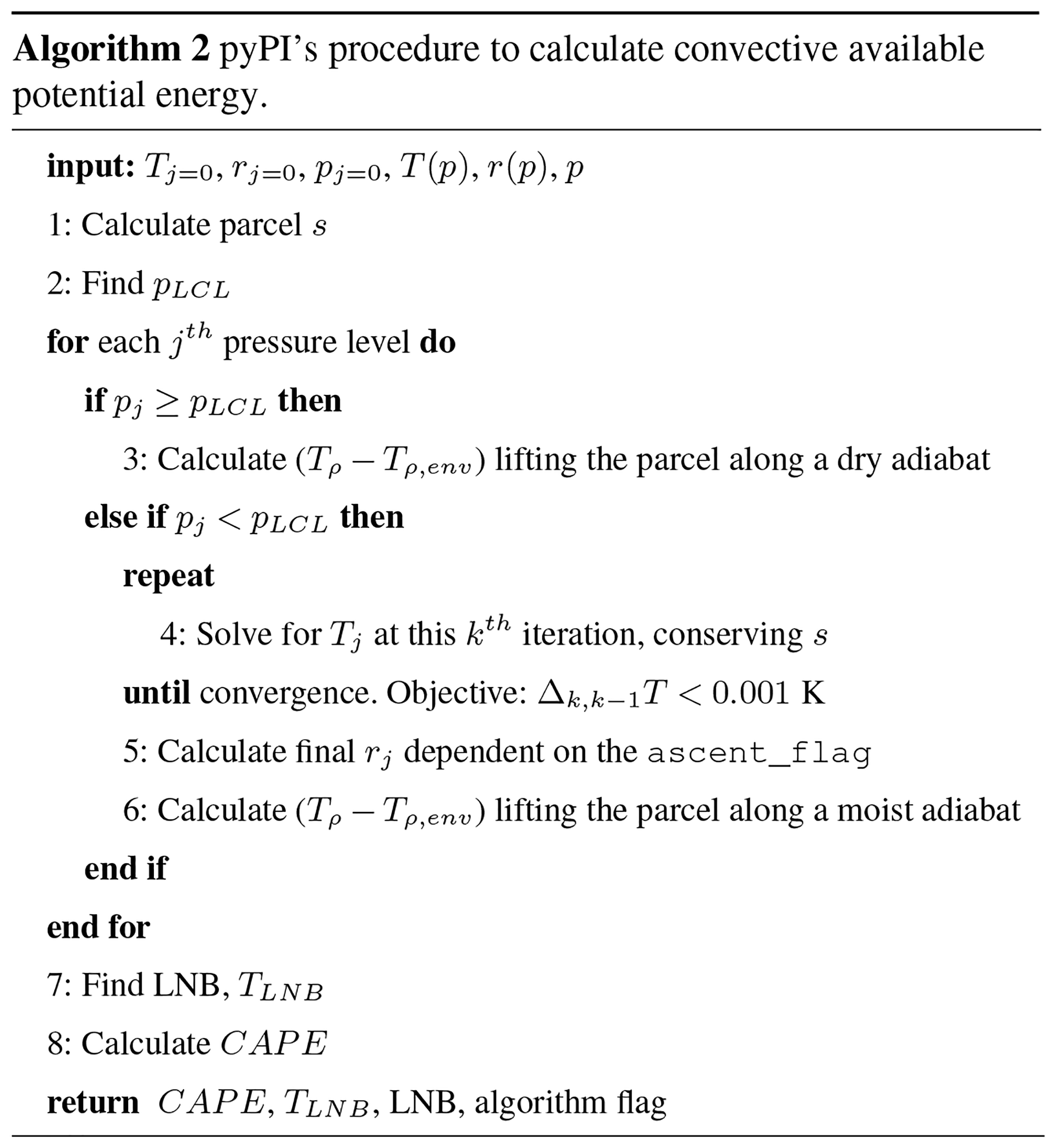
Given an initial surface parcel temperature, pressure, and mixing ratio, the procedure begins by finding the parcel's reversible entropy, which is conserved as it is lifted on the sounding. The parcel's water vapor pressure is found via the ideal gas law (e.g., Bolton, 1980, their Eq. 16):
Saturation vapor pressure (in hPa) is given empirically as a function of T in degrees Celsius by Bolton (1980), their Eq. (10), following the Clausius–Clapeyron relation:
Then fractional relative humidity is defined as . Assuming the temperature dependence of specific heats is negligible over the range of temperatures in the tropical atmosphere and integrating Kirchhoff's equation (e.g., Emanuel, 1994, Eqs. 4.4.3–4.4.4), the temperature dependence of the latent heat of vaporization is
with T in degrees Celsius. Finally, we are equipped to calculate the parcel's reversible total specific entropy (per unit mass of dry air), s, which is conserved as the parcel is lifted along the sounding (Emanuel, 1994, their Eq. 4.5.9):
where rT is the total water content mixing ratio, which is identical to the parcel mixing ratio at the surface.
Having determined the parcel's initial moisture properties, we next find the lifting condensation level (LCL) of the parcel, in order to partition the upcoming buoyancy calculation between saturated and unsaturated regions of the profile. The pressure of the LCL, pLCL, is found empirically with3
where A=1669 and B=122. Note that the LCL of a lifted parcel that is
already saturated is identical to its original pressure level,
i.e., pLCL≡p. Likewise, parcels at levels below the LCL are
(by definition) not saturated. After finding pLCL the CAPE
algorithm begins an “updraft loop”, where the positive and negative buoyancy
of the parcel is calculated at every jth pressure level below the upper
boundary on pressure (ptop, Sect. 4.1).
Starting with calculations at levels below the LCL (pj>pLCL), at each jth level the algorithm calculates the unsaturated parcel temperature by following a dry adiabat with the same temperature as the surface parcel. Applying Poisson's equation,
Because CAPE is proportional to the positive and negative areas enclosed by the environmental and lifted parcel density temperatures (Tρ,env and Tρ, respectively), we calculate the density temperature as (Emanuel, 1994, their Eq. 4.3.6)
where the net water mixing ratio (rT) is the same as the parcel water mixing ratio at the surface and in the environment below the LCL before condensation has occurred (i.e., rT≡rj=0 and ).
Next the algorithm finds the density temperature differences for all levels
above the LCL (pj<pLCL). Because the parcel is saturated
above the LCL, its moisture characteristics and temperature must be found
iteratively at each jth level. First the algorithm solves for r by
rearranging Eq. (4); then until the numerical iteration converges
(with objective for the parcel temperature: ΔT<0.001 K) it
solves for parcel moisture characteristics which conserve the parcel's
specific entropy s (Eq. 7) following a moist adiabat;
finding these permits an estimation of the density temperature differences at
each level. At the beginning of the loop, T and r are set equal to the
previous iteration's findings; then the loop steps forward updating the
parcel's temperature (and the dependant Lv and water vapor
mixing ratios) assuming s is conserved following saturated reversible
adiabatic displacement. Following Newton's method (; Wallis, 1685), when the difference between
s and this iteration's entropy, sk, scaled by the rate of change of
entropy with temperature, sℓ, is small
(i.e., ), the algorithm will
converge to estimate the parcel temperature at this level, Tj. Here
AP is a numerical step size employed to speed convergence, which
changes dynamically depending upon the number of iterations that have taken
place. If at any given level the total number of iterations exceeds 500 (an
excessive number of iterations), or if the water vapor pressure becomes
unrealistically close to the level pressure, then the algorithm fails to
converge and returns zero CAPE.
When the algorithm converges for a level, the final parcel mixing ratio is set
depending on the ascent type chosen by the user (Sect. 4.1). For
pseudoadiabatic ascent (ascent_flag = 1), liquid water condensed in
the parcel during its ascent is assumed to drop out of the parcel, such that
the heat capacity of liquid water is neglected and the mixing ratio is a
function of the final level temperature (i.e., rj=r(Tj)). For reversible
ascent (ascent_flag = 0) the total water (and its heat capacity) is
retained following the parcel (i.e., ). For intermediate
fractions of ascent_flag, the mixing ratio scales over r(Tj)→rT.
Note that the density temperature difference (and hence a parcel's buoyancy) with height is not strictly higher under either ascent assumption. Parcels lifted reversibly are always warmer than those lifted psuedoadiabatically, but the weight of the carried condensate also means these parcels are more dense until they reach the upper troposphere (Emanuel, 1994, their Table 4.2). Accordingly, Gilford et al. (2017) found that psuedoadiabatic (typically more buoyant) PI calculations generally have higher altitude OTLs than reversible (typically less buoyant) PI calculations on monthly timescales.
Having determined rj, the algorithm computes the density temperature for the parcel and the environment (Eq. 10) and calculates each level's density temperature differences, . We are now equipped to calculate the lifted parcel's convective available potential energy. CAPE is given by the vertically integrated buoyant energy between the level from which the parcel is initially lifted (j=0) and the level of neutral buoyancy (LNB; j=LNB). Following Emanuel (1994), their Eq. (6.3.6),
where
Negative areas (NA) are vertical regions of negative buoyancy which inhibit spontaneous convection in the profile; positive areas (PA) are vertical regions of positive buoyancy which cause the parcel to rise assuming an initial upward displacement. Note that CAPE is not defined for parcels without positive areas. By definition, the level of free convection (LFC) separates regions that are negatively buoyant (below) from regions that are positively buoyant (above). When , the regions of the profile above the LCL and below the LFC may still be negatively buoyant.
The CAPE algorithm numerically solves Eqs. (11)–(13) in five steps.
First, we find the maximum level of positive buoyancy (INB), i.e., the
highest altitude jth level where . If
this highest level remains at j=0, then there are no positively buoyant
levels and the function returns zero CAPE.
Second, noting that at each layer over the levels j and j+1 – where the average pressure of each layer is – we find the positive and negative areas between the second-highest altitude level (i.e., j=1) and the the maximum level of positive buoyancy.
Third, we find the residual negative area (if ) or positive area (if ) of the mean layer composed of the surface and the lowest level.
Fourth, we find the LNB and the temperature at the LNB, TLNB,
along with the residual positive area of the mean layer between the
maximum level of positive buoyancy and the LNB. If the INB is found
at the highest valid level (constrained by ptop,
Sect. 4.1), then the LNB and TLNB are set at that
level.
Finally, the negative and positive areas are added together with the residuals following Eq. (11). After this last step, the algorithm flag is set to indicate the algorithm has successfully computed CAPE. Then the values of CAPE, TLNB, the LNB, and the flag are returned to the PI module.
A caveat of this approach is that different thermodynamic profile analysis routines – and especially CAPE calculations – can produce results which vary substantially from one another (e.g., Blumberg et al., 2017). The routine presented here contrasts with those of other Python modules such as MetPy (May and Bruick, 2019) and SHARPpy (Blumberg et al., 2017), particularly in the pLCL estimate, the feature to scale between psuedoadiabatic and reversible ascent, and the vertical integration of density temperature differences when evaluating CAPE (compared to the traditionally used temperature or virtual temperature vertically integrated differences; e.g., Doswell and Rasmussen, 1994). More work is needed to determine the sensitivity of pyPI to thermodynamic assumptions and functional forms (Appendix B); in the context of potential intensity it is the CAPE difference that is most important (Eq. 2), which may limit the PI sensitivity (as long as the routines used remain internally consistent). While beyond the scope of this study, pyPI's framework could enable further investigation into this and related model sensitivities.
3.3 PI module
The PI module begins by checking to ensure that the input atmospheric profile is appropriate for the PI calculation. If not, missing values are returned by the algorithm (see Sect. 4.2). Water vapor mixing ratios above the boundary layer do not influence the PI calculation (they are redundant in ), so any missing r values above the surface are replaced with 0 g kg−1.
Following Algorithm 2 described above, pyPI computes CAPEenv, assuming the environmental air parcel is lifted from the lowermost input level in p.
Next, pyPI iteratively solves Eqs. (2) and (3) (with objective4 for the minimum pressure at the RMW: hPa). The algorithm begins by calculating the convective available potential energy (computing Algorithm 2 at each ith iteration) iterating from the initial lowest-level environment inward toward the radius of maximum winds, CAPE|RMW. At each iteration the mixing ratio is updated to account for pressure dependence (r increases slightly as p→pm approaching the RMW; Bister and Emanuel, 2002).
Next, we calculate the saturation convective available potential energy at the radius of maximum winds, CAPE*. This calculation assumes the parcel is lifted directly from the sea surface, such that T=Ts and r=rs(Ts) (where rs is found given Ts via Eqs. 5 and 4). pyPI defines the outflow temperature level (OTL) and T0 as the LNB and TLNB found during the final iteration of CAPE* computation, respectively. Note that the OTL and T0 could instead be found during the final iteration of the CAPEenv computation. Flexibility in the outflow definition is a planned improvement for pyPI. The choice to use CAPE* follows from defining the outflow level with a fully saturated parcel lifted directly from the sea surface (see Sect. 6.2).
The ratio of sea-surface and outflow temperatures in Eq. (2)
represents the scaling of PI by dissipative heating, which increases PI when
(Bister and Emanuel, 1998). At each iteration this
ratio is set with the fixed input Ts and the current T0≈TLNB. The relevance of this ratio for the PI calculation is
set by the user with the adjustable parameter diss_flag
(Sect. 4.1). If dissipative heating is permitted to impact the
tropical cyclone potential intensity (diss_flag = 1), then the ratio
remains as defined above. If dissipative heating is not considered
(diss_flag = 0), then the algorithm assumes
![]() in the following
calculations.
in the following
calculations.
Next, pm is estimated in each iteration following Eq. (3). The surface environmental virtual temperature, Tυ, is found as the average of virtual temperatures over the mean layer composed of the parcel (with temperature, Ts) and the lowest level, i.e., . The virtual temperature is identical to the density temperature (Eq. 10) at the surface (as rT=r(Ts)) and may be approximated at the lowest level with . Combining Eqs. (2) and (3) to solve for pm, the algorithm iterates towards a new pressure estimate. If the number of iterations exceeds 200 (an excessive number of iterations), or if the estimated pressure drops below an unphysical 400 hPa, then the PI algorithm fails to converge and returns missing outputs.
When the algorithm has successfully converged on a stable value of pm, the final central minimum pressure, pmin, is set. Assuming cyclostrophic balance and that the azimuthal velocity in the eye is given by , we follow a power law scaling with exponent b (see also Emanuel, 1995, their Eqs. 25–26):
where pyPI assumes following Bister and Emanuel (2002) that b=2.
Note that the difference, , is typically small. Historically, when CAPEenv was used to compute PI in the final term of Eq. (2), it was found to add noise to the PI algorithm output (Kerry Emanuel, personal communication, 2020). Therefore, pyPI instead replaces this term with in the PI computation for tractability. PI calculations with the original Bister and Emanuel (2002) formulation have identical OTLs and outflow temperatures but tend to have higher Vmax values by between 0 and 32 m s−1 (not shown). Global and tropical (20∘ S–20∘ N) mean biases from this approximation are ∼3 and ∼2.5 m s−1, respectively.
Finally, we may find tropical cyclone potential intensity. Assuming that the
raw computed maximum gradient wind speeds are scaled to 10 m winds
with some fraction, we multiply the result from Eq. (2) by V_reduc
(Sect. 4.1). This step completes the PI computation. The module
sets the flag to indicate the successful computation of pyPI's algorithm and
then outputs Vmax, pmin, the flag, T0, and the OTL.
pyPI (v1.3) is written in Python v3.7 and its calculations are optimized with Numba (Lam et al., 2015). An average model elapsed run time (on a laptop) is ∼10 s per 100 000 input profiles. This is ∼18 % slower than the mean run time of the BE02 MATLAB algorithm (on the same machine); however, pyPI is now appropriately handling missing input data (Sect. 4.2) which increases its run time relative to the MATLAB algorithm. We stress that run times will ultimately depend a user's particular implementation and computing resources.
Modeling the maximum intensity of a tropical cyclone with pyPI requires input environmental state variables: temperature (T) and mixing ratio (r) profiles on pressure levels (p), as well as concurrent Ts and mean sea-level pressures (pmsl). Algorithm variables and parameters are shown in Table 1.
4.1 Adjustable parameters
pyPI includes six adjustable parameters that may be set in the module call, with the caveat that each should be chosen within the defined “Values” column of Table 1. Parameters set outside these values could result in syntax errors or logical errors in the output or may give rise to unphysical PI estimates.
4.1.1 CKCD (default = 0.9)
The ratio is an uncertain constant which depends on the sea state and linearly scales potential intensity; its value is an ongoing area of field and theoretical research (Emanuel, 2003). Table 1 includes the 1σ range of the ratio found with energy and momentum budget methods by the 2003 Coupled Boundary Layers Air–Sea Transfer (CBLAST) field program (Bell et al., 2012); numerical studies have also probed the sensitivity of simulated tropical cyclones to these exchange coefficients (Bryan, 2012; Green and Zhang, 2014). Studies exploring PI variability typically use a default value of when calculating PI (e.g., Wang et al., 2014; Wing et al., 2015).
4.1.2 ascent_flag (default = 0)
The ascent process proportion determines whether the air parcels displaced in
each CAPE calculation (cf. Sect. 3.2) follow
reversible adiabatic ascent (ascent_flag = 0) or pseudoadiabatic
ascent (ascent_flag = 1). In the case of reversible ascent, the
full moist entropy of the buoyant parcel is conserved along its displacement
following a moist adiabat. In pseudoadiabatic ascent the heat capacity of
liquid water is neglected. Liquid water is assumed to fall out of the parcel
as it condenses, while the parcel ascends following the pseudoadiabatic moist
adiabat; for more details see Emanuel (1994), their Sect. 4.7. For
practical applications of pyPI, ascent_flag may be set to any value
between 0.0 and 1.0, such that the proportion of ascent is any fraction
intermediate to fully reversible and fully pseudoadiabatic ascent.
4.1.3 diss_flag (default = 1)
The dissipative heating flag determines whether dissipative heating is
accounted for (diss_flag = 1) or ignored
(diss_flag = 0) in potential intensity theory (see
Bister and Emanuel, 1998, their Eq. 22). When dissipative heating is included in
the PI calculation, the leading factor in the BE02 algorithm
(Eq. 2) is ,
where . In the absence of dissipative heating,
the leading factor is following the original findings of
Emanuel (1986, 1995). Scaling arguments and empirical estimates
suggest that dissipative heating increases PI by about 20 %–30 %
(not shown).
4.1.4 V_reduc (default = 0.8)
Raw potential intensities are maximum gradient wind speeds
(Emanuel, 2000). Therefore, gradient winds calculated with the BE02
algorithm are not directly comparable with observed intensities at the
near-surface without applying an approximate scaling between gradient and
10 m winds. Following Powell (1980), a crude reduction of
20 % (V_reduc = 0.8) is typically applied to scale PI
for comparison with near-surface winds. The percent reduction in the gradient
wind in terms of V_reduc is
. Note that for some
applications of PI, such as using it as a thermodynamic parameter in climate
science – e.g., incorporation into the genesis potential index,
Camargo et al. (2007) – V_reduc should be set to 1.0 (no reduction).
4.1.5 ptop (default = 50)
The upper level pressure bound is the minimum pressure below which the input
profile is ignored during PI computation. Theoretically modeled tropical
cyclone outflow can often exceed the tropical tropopause on climatological
timescales (Gilford et al., 2017), so setting ptop > 100 hPa it
is not advisable. Reducing the number of considered levels by increasing
ptop may potentially increase the speed of calculations, at the risk
of finding an unrealistically low-altitude OTL and too warm a T0. Before altering ptop,
users should consider their particular application and the outflow levels they
anticipate given the stability of their input profiles.
4.1.6 miss_handle (default = 1)
The missing data flag prescribes how missing values are handled in the
CAPE calculation (discussed below). Following the BE02 MATLAB code
(miss_handle = 0), if missing values are found in the input
temperature profile, then the algorithm will attempt to calculate PI for all
available levels above the missing values. However, the user may also
conservatively choose that any missing values in the input profile will
immediately set the entire PI calculation output to missing
(miss_handle = 1).
4.2 Handling missing data
Mirroring the output flag convention of the BE02 MATLAB code,
IFL = 1 when the PI algorithm successfully returns valid
potential intensity outputs, IFL = 0 when the algorithm fails
because the input data are improper for a PI calculation (e.g., if
), and IFL = 2 when the
algorithm fails to converge.
One major difference between pyPI and the BE02 MATLAB algorithm is the handling of missing data and the (related) flag provided in the output. By convention, missing input variables in pyPI are assigned Python's “Not a Number”, NaN, to avoid errors. The BE02 MATLAB code default is that profiles may contain missing values (specifically temperatures on pressure levels), and the algorithm computes PI over the remaining valid levels.
Because missing values may sometimes be found at the surface – and the primary CAPE calculation (Sect. 3.2) relies heavily on the assumption of lifting the parcel within the storm and environment from that level – errors could arise from estimating PI when ignoring near-surface buoyancy. In principle, PI should be calculated only over data points with existent sea-surface temperatures and lowest profile level temperatures. In practice, missing data may arise at the lowest profile level, which would lead to errant PI calculations if these profiles are input to the BE02 MATLAB code.
pyPI addresses this challenge in three ways. First, an adjustable parameter
(miss_handle) is implemented to allow the user to specify how pyPI
handles the missing values. If miss_handle = 0, the code
attempts to handle missing values akin to the way that the BE02 MATLAB code
did, although there still remain some differences in the outputs between pyPI
and the MATLAB algorithm. Specifically, pyPI's CAPE calculation
proceeds as normal only as long as there are no missing values between the
lowest valid (non-missing) level and the OTL; otherwise, CAPE module
outputs (and hence PI module outputs) are returned as missing. Second, if
miss_handle = 1, then the CAPE function will
automatically interpret temperature profiles with missing data as invalid and
return missing values to the PI algorithm, resulting in the PI outputs being
set to missing in the return. Third, a new output flag value
(IFL = 3) is introduced in pyPI which is returned when missing
values in the temperature profile results in a missing output return from the
PI module (i.e., in either of the two cases described above), which aids in
interpreting pyPI output.
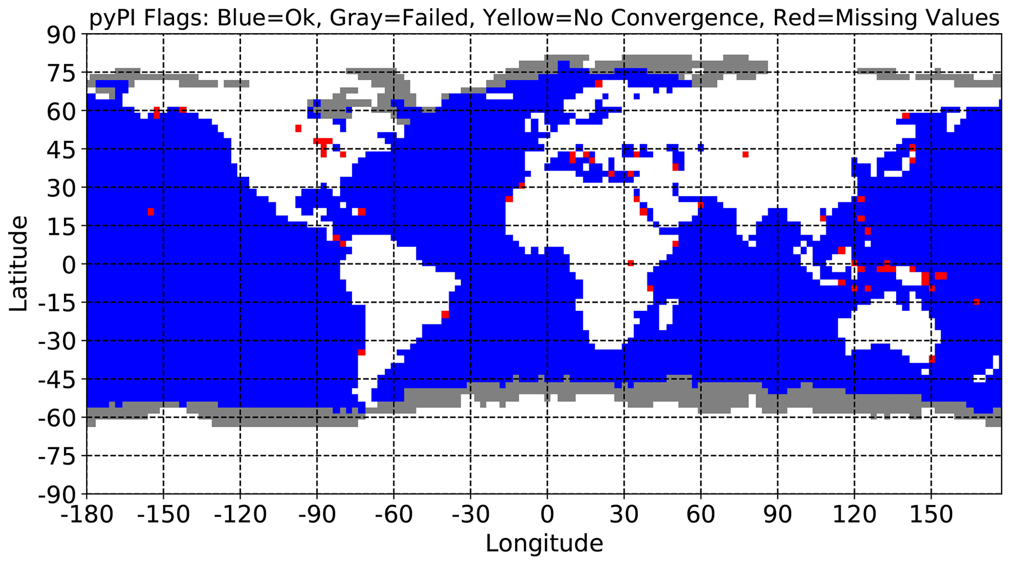
Figure 2pyPI status flags from September 2004 potential intensity calculations when miss_handle = 1. Blue grid cells indicate the PI algorithm converged, gray grid cells indicate the PI algorithm failed to pass a check, yellow grid cells indicate the PI algorithm did not converge, and red grid cells indicate the PI algorithm failed due to missing profile data.
Figure 2 shows an example of the output algorithm status flags from pyPI
calculations with a single month's mean environment (September 2004) from
MERRA2 data (Sect. 5.1), and with the default
miss_handle = 1. The figure illustrates the few global points
which had at least some missing data, resulting in a missing PI return from
pyPI (IFL = 3; red grid points). In contrast, these locations
have an output (but likely errant) PI from the BE02 MATLAB code. The majority
of locations where missing input data results in missing output PI are near
land (e.g., the Caribbean and Indo-Pacific), where missing values arise as an
artifact of the differences between the sample data and the land–sea mask
applied (Sect. 5.1). Missing values in the sample data (which has
lowest data pressure level of 1000 hPa) could also be in locations
where the monthly average pmsl is below 1000 hPa,
resulting in T(1000 hPa)=NaN.
In the example pyPI calculation (Fig. 2) there are no inputs for which the algorithm does not converge (cf. Bister and Emanuel, 2002). One final complication is that BE02 MATLAB code occasionally returns Vmax=0 as an output. In these cases, pyPI instead returns Vmax=NaN.
pyPI outputs valid (non-missing) potential intensities over ∼65.6 % of the ocean grid points in the global 2004 sample dataset –
compared with ∼64.41 % returned by the BE02 MATLAB code. In
addition to how missing data are handled, output differences may also arise
from slight variations in numerical computation between Python and
MATLAB. pyPI validation tests (Sect. 5) are computed over
all spatiotemporal locations for which both algorithms have
non-missing/non-zero potential intensities (and with
miss_handle = 1).
4.3 Opportunities for scientific improvement
In addition to updating the original BE02 algorithm, pyPI is designed with the intention to undergo further scientific developments as requested or created by the community. In addition to including alternative intensity indices (e.g., Lin et al., 2013; Rousseau-Rizzi and Emanuel, 2019), potential pyPI improvements generally fall into two broad categories.
Increased model flexibility. Such improvements would alter the code to provide users more parameter choices when the PI module is called, through either input flags or additional variables. For instance, users may want to select between the CAPE definition used to estimate pmin in Eq. (14) (i.e., CAPE|RMW or CAPEenv) or explore alternative outflow temperature definitions (e.g., setting TLNB during the computation of CAPEenv compared with the default CAPE* calculation).
Incorporation and/or development of fundamental or incremental scientific advances. As the scientific understanding of tropical cyclone intensity and potential intensity increases, such knowledge could be brought into pyPI. For instance, Kieu and Wang (2017) showed that the assumption of moist neutrality in calculating PI may not be appropriate, even when a cyclone is mature. Multiplying Eq. (2) by a factor of in the pyPI codebase, where Γ is the environmental lapse rate and αΓ is an empirical parameter, would enable further exploration of how stratification affects PI.
A specific goal for future pyPI development is to replace the current empirical estimate of pLCL with a modern formulation (e.g., Romps, 2017). Other opportunities for improvement might be more involved, requiring significantly more research to implement. For example, the magnitude of is nonlinearly related to wind speed (Nystrom et al., 2020); a mathematical relationship between wind speed and this ratio could in principle be incorporated into potential intensity theory, but this would require revisiting PI theory and further theoretical advancements before inclusion within pyPI.
These examples are not exhaustive but show the range of possibilities for future pyPI development and the potential future value of this model in the tropical meteorology community.
5.1 Sample reanalysis data
The pyPI sample data are monthly means of state variables from the second Modern-Era Retrospective Analysis for Research and Applications (MERRA2, Gelaro et al., 2017) in 2004, interpolated onto a global grid. Note that for these example pyPI calculations the water vapor mixing ratio, r, is approximated by substituting in the reanalysis specific humidity, q (as , because r≪1).
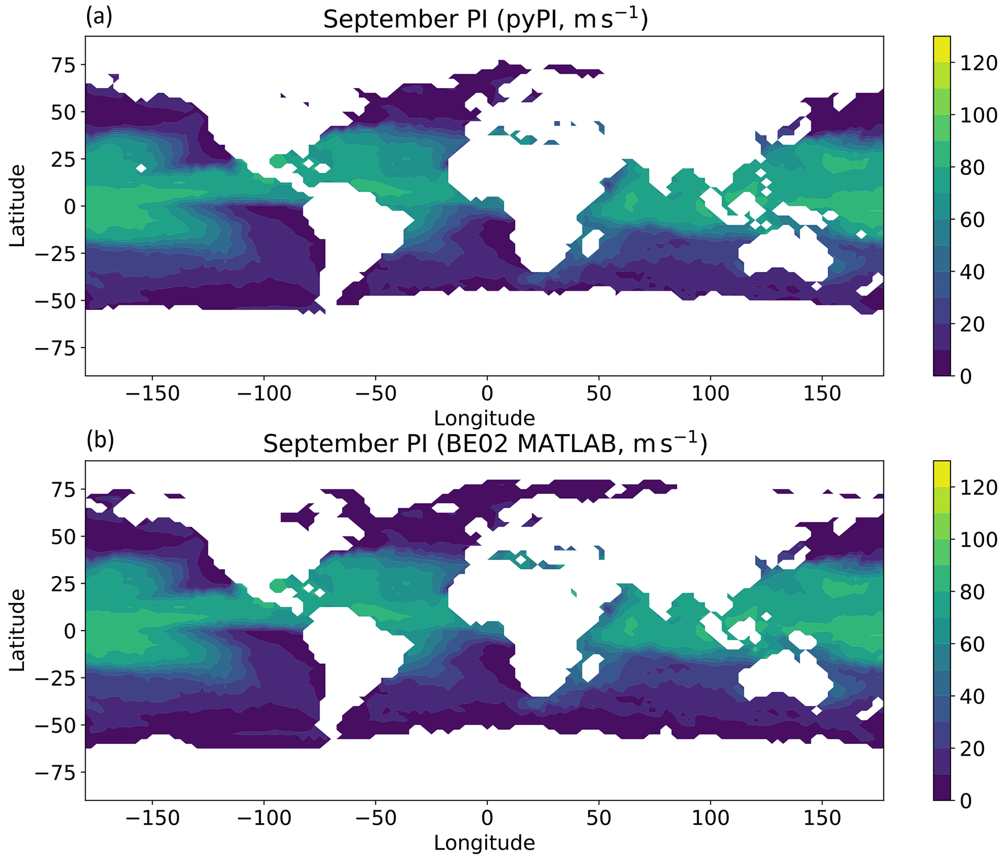
Figure 3September 2004 mean potential intensities (m s−1) calculated with pyPI (a) and the BE02 MATLAB code (b).
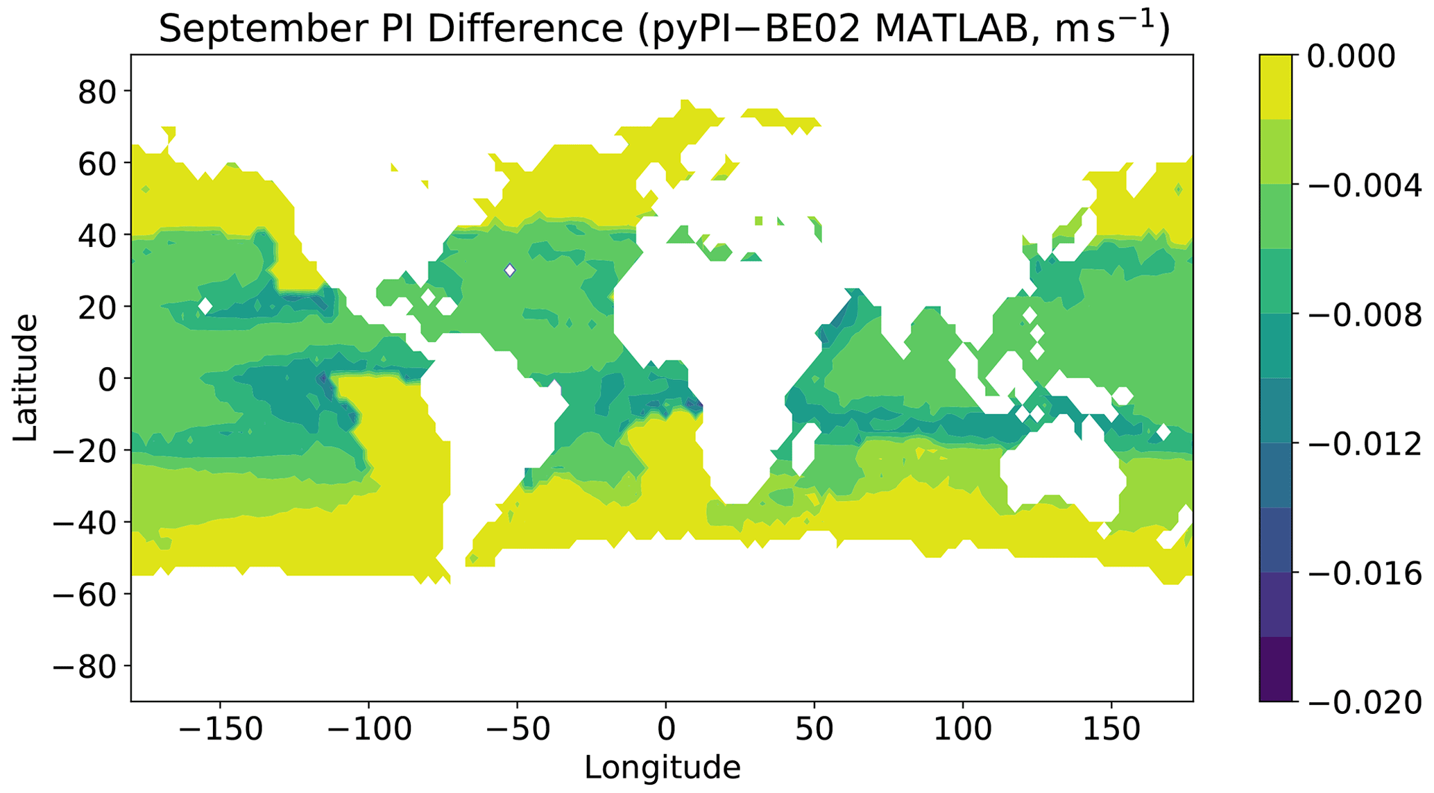
Figure 4September 2004 mean potential intensity differences (m s−1) between those calculated with pyPI minus those calculated with the BE02 MATLAB code.
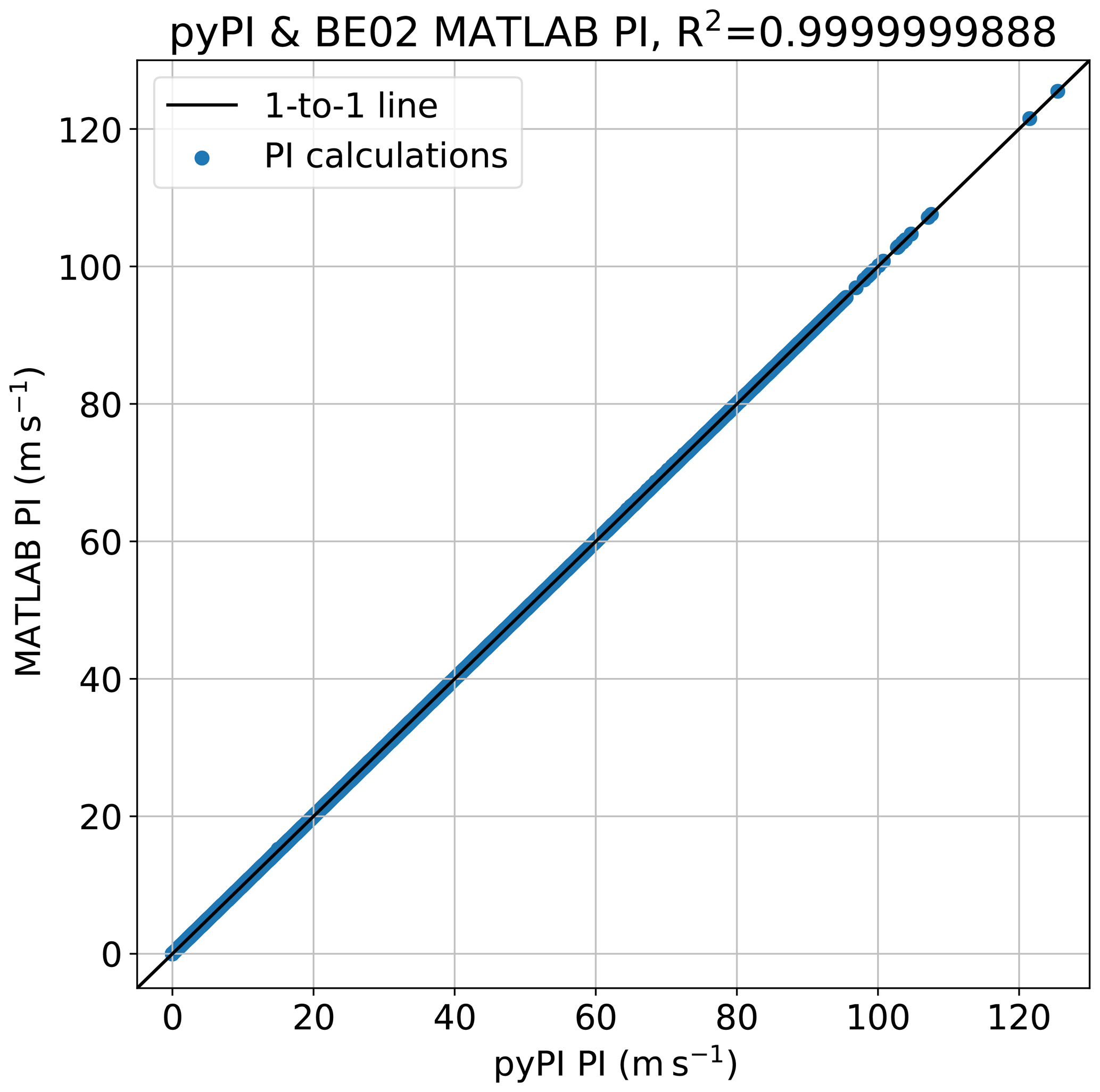
Figure 52004 mean potential intensities (m s−1, blue dots) calculated with pyPI (horizontal axis) and the BE02 MATLAB code (vertical axis). The black curve is the 1 : 1 line.
Potential intensity calculations are generally linear (i.e., mean potential intensities may be estimated as a function of mean environmental variables):
where E[ ⋅ ] is the expected value of a function or variable. Using monthly mean environmental conditions – instead of 6-hourly observations – to compute climatological monthly means of potential intensity (and the algorithm's other output variables) generates a small bias of <1 m s−1 globally and <0.5 m s−1 in the tropics. PI's linearity property is convenient, because it reduces the scale of data needed to compute PI: daily or hourly data are not needed for monthly or longer (climatological) applications. Applications on shorter (e.g., operational or daily) timescales, however, should use appropriately shorter frequency inputs to the pyPI algorithm.
The sample data uses the land–sea mask from the European Centre for Medium-Range Weather Forecasts Interim (ERA-Interim, Dee et al., 2011) on a global grid. By definition, Vmax≡0 where Ts=NaN (i.e., over land); in some cases (e.g., if skin temperatures valid over land are used in lieu of sea-surface temperatures) PI may be mistakenly calculated over land with the PI module. In these cases, users should assign all PI algorithm outputs over land to the missing value in post-processing. As an alternative, in this pyPI example input variables over land are set to missing in a pre-processing step. Note that the mismatch between using the ERA-I land–sea mask and MERRA2 data in this example results in a set of minor output artifacts caused by missing (MERRA2 land grid points) input data over ERA-I defined ocean grid points. This artifact provides a useful demonstration of the missing data flag employed in pyPI (Sect. 4.2).
5.2 Validating against the BE02 implementation
Accompanying the environmental conditions in the sample data are outputs from the BE02 MATLAB code written by Kerry Emanuel (Bister and Emanuel, 2002). Potential intensities calculated over September 2004 with pyPI and the extensively used BE02 MATLAB code are compared in Fig. 3 over the globe; their difference is computed and plotted in Fig. 4. There is excellent agreement between the two algorithms; 98.5 % of output potential intensities have absolute differences <0.01 m s−1. Potential intensities calculated with the Python algorithm exhibit a slightly negative bias relative to the MATLAB calculations, but these differences are negligible compared with other uncertainties in the PI calculation, such as the ratio of surface exchange coefficients (Table 1).
Figure 5 shows the scatter between all potential intensity values calculated with the two algorithms over the sample data, plotted against a 1 : 1 line (values lying on this line exhibit perfect agreement). The R2 of this comparison is R2≈1.0 to seven significant digits, such that the calculations are nearly identical. All other output variables (cf. Table 1) from the two algorithms have similarly strong levels of agreement.
A minor PI difference between pyPI and the BE02 MATLAB algorithm arises when the pyPI-found outflow level has a higher pressure and warmer temperature than found by the BE02 code. The outflow property differences result from pyPI's correction of a minor error that was present in the BE02 algorithm, where ϵ was defined as 0.622 rather than directly calculated as . The small rounding error results in a handful of profiles with lower altitude outflow and lower PI values calculated by pyPI. In the absence of correcting this error, the correlation between the two calculations is R2≈1.0 to 13 significant digits, and the absolute maximum difference anywhere is m s−1.
I conclude that the PI calculations made with the pyPI algorithm are adequately validated against the BE02 MATLAB code, and that pyPI is sufficiently accurate for use in research applications.
6.1 Annual mean PI
Figure 6 shows 2004 annual mean sea-surface temperatures, as well as pyPI-calculated potential intensities, outflow temperatures, and outflow temperature levels. The familiar pattern of warm SSTs in the tropics corresponds with high Vmax values, suggesting that on an annual timescale PI is strongly influenced by Ts. These warm and high-PI regions are accompanied by outflow temperature levels with annual pressures below 100 hPa, deep in the tropical tropopause region (e.g., Fueglistaler et al., 2009). Near the tropical tropopause, annual mean outflow temperatures are remarkably cold, around 200 K. On average, the coldest outflow temperatures are found in the western North Pacific basin, where consistent deep convection and stratospheric circulation act to keep tropopause temperatures very cold and highly variable (e.g., Randel and Jensen, 2013).

Figure 62004 annual mean potential intensities in (a), sea-surface temperatures in K (b), outflow temperatures in K (c), and outflow temperature levels in hPa (d) calculated with pyPI.

Figure 72004 seasonal cycles of potential intensity in meters per second (a), sea-surface temperature in K (b), outflow temperature in K (c), and outflow temperature level in hPa (d) calculated with pyPI and averaged over the main development regions: the North Atlantic (red), eastern North Pacific (green), western North Pacific (blue), North Indian (yellow), and Southern Hemisphere (black).
6.2 PI seasonal cycles
A slightly more sophisticated application of pyPI is the calculation of potential intensity seasonal cycles. Reproducing the methodology of Gilford et al. (2017) with pyPI calculations over 2004, Fig. 7 shows the seasonal cycles of sea-surface temperatures, as well as outflow temperatures, outflow temperature levels, and potential intensities in 2004 averaged over tropical cyclone main development regions (defined in Gilford et al., 2017, their Table 1).
The seasonal cycles of PI are known to be quite robust year over year and exhibit clear differences between regions. The western North Pacific has a nearly flat seasonal cycle of PI, while the other basins are more intraseasonally variable. While the muted sea-surface temperatures certainly play an important role in this damped cycle, the outflow temperature pattern is typical of the cold-point tropopause seasonal cycle (e.g., Yulaeva et al., 1994; Randel and Wu, 2014) – which the OTLs are reaching – which acts to damp the seasonal cycle further by decreasing PI in the boreal summer and increasing PI in the boreal winter. As a result, tropical cyclones in the western North Pacific have higher speed limits during the boreal winter months. Consistent with this finding, historical observed typhoons show intense wind speeds during the winter and spring months (Gilford et al., 2019). For example, in early April 2004 Typhoon Sudal reached Category 4 strength, ∼67 m s−1, when the co-located monthly average PI was about 75 m s−1.
The seasonal cycles of each basin illustrate the complex relationship between sea-surface temperatures, OTLs, and outflow temperatures. Figure 8 diagrams this relationship in more detail, showing how one assumption in the pyPI algorithm impacts the output PI values. pyPI assumes that the outflow temperature and its level are derived by finding the LNB assuming a saturated parcel lifted from the sea-surface with temperature, Ts. This implies that, following a moist adiabat, the level of the neutral buoyancy is a function of only Ts and the environmental temperature profile, T. Given a fixed temperature profile, a 3 ∘C increase in Ts (e.g., from SST1 → SST2 in Fig. 8) requires that the associated OTL will be found at a higher altitude (OTL1 → OTL2 in Fig. 8), and the associated outflow temperature will likewise change. As the atmosphere's stratification increases into the lower stratosphere, increases in Ts become less effective at changing the OTL and its temperature, with the effect nearly saturating when the outflow reaches the cold-point tropopause (e.g., 100 hPa in Fig. 8). At this point, T0 variability is almost completely decoupled from Ts variability. Instead these T0 values become influenced by tropopause region variability (e.g., Emanuel et al., 2013; Ramsay, 2013; Wang et al., 2014; Wing et al., 2015; Gilford et al., 2017) which is controlled by radiation, dynamics, and deep convection (e.g., Fueglistaler et al., 2009; Randel and Wu, 2014).
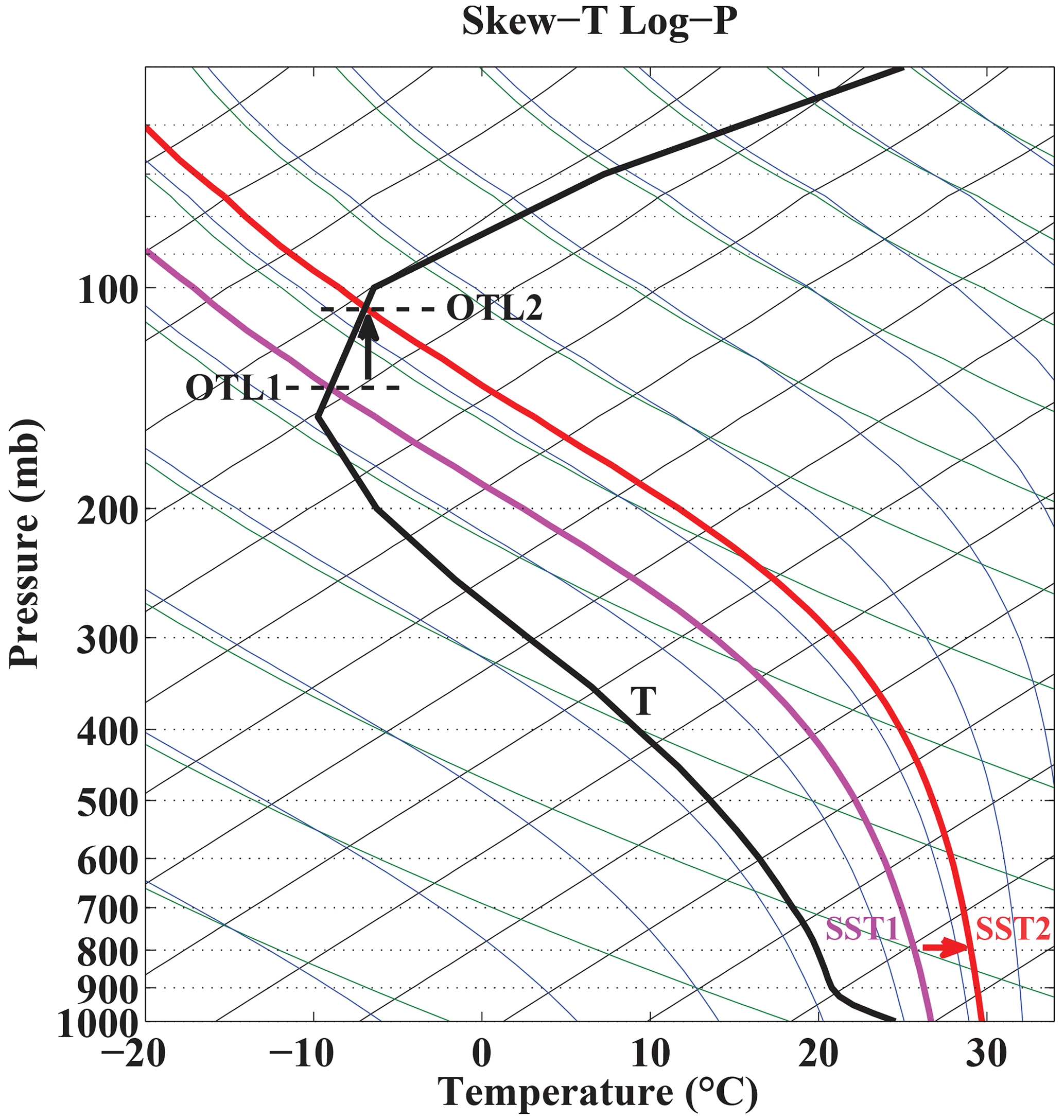
Figure 8Skew-T log-P thermodynamic diagram with isotherms (thin black curves), dry adiabats (green curves), and moist adiabats (blue curves). The bold black line is a mean environmental temperature profile from the North Atlantic main development region, the magenta curve is the moist adiabat associated with a mean North Atlantic sea-surface temperature (SST), and the red curve is the moist adiabat associated with a sea-surface temperature 3 ∘C warmer than the mean.
These properties are borne out in the example 2004 seasonal cycles computed in Fig. 7. In the North Atlantic basin sea-surface temperature and OTL seasonal cycles are inversely proportional: colder sea-surface temperatures have higher-pressure OTLs and warmer outflow temperatures found in the upper troposphere (where ) in all months except August–September. In these late summer months the OTL reaches near the cold-point tropopause, and the outflow temperature slightly increases, following the seasonal cycle of warmer tropopause temperatures (e.g., Yulaeva et al., 1994). A contrasting pattern is observed in the western North Pacific, where OTLs have almost no seasonal cycle: in this basin the calculated outflow always reaches the lowermost stratosphere (OTL ≤90 hPa). Accordingly, the outflow temperature seasonal cycle perennially follows the seasonality of lowermost stratospheric temperatures, which minimize in the boreal winter and maximize in the boreal summer (Yulaeva et al., 1994). Comparing with Eq. (1), this T0 seasonality leads to relatively increased PI values in the boreal winter and relatively decreased PI values in the boreal summer. Overall, the PI seasonal cycle in the western North Pacific is damped over the year, a pattern that is observed in real-world tropical cyclone intensities (cf. Gilford et al., 2019).

Figure 9Seasonal amplitudes of each PI decomposition term (Eq. 16) in 2004 and each main development region, calculated with pyPI. Compare with Gilford et al. (2017), their Table 2. By convention, negative amplitudes indicate the associated seasonal cycle peaks in the boreal winter. For reference, the dashed black line indicates the magnitude and sign of the seasonally invariant log.
6.3 Decomposition analysis
The relative contributions to potential intensity may be mathematically derived by decomposing Eq. (1). Taking the natural logarithm of both sides,
Then PI variability is related to variability in either tropical cyclone efficiency () or thermodynamic disequilibrium (); recall that is taken as a constant. As an example, Eq. (16) is applied to pyPI-calculated 2004 seasonal cycles of potential intensity (from Fig. 7). pyPI calculates PI directly, and efficiency may be directly computed from input Ts and output T0; following Wing et al. (2015) the disequilibrium term is taken as a residual from Eq. (16).
After finding each term in Eq. (16) over each basin and seasonal cycle, the amplitude (defined as the annual range evaluated with monthly observations) of each seasonal cycle is plotted in Fig. 9. By convention, a negative amplitude indicates the approximately sinusoidal seasonal cycle reached its maximum in the boreal winter and minimum in the boreal summer.
In all basins, the disequilibrium term drives the largest portion of the seasonal amplitude. This is consistent with sea-surface temperature seasonal cycles which dominate the disequilibrium variance (Fig. 7). The efficiency term is smaller, and in each basin it follows the same cycle as thermodynamic disequilibrium, with the exception of the western North Pacific (where the efficiency seasonal cycle maximizes in the boreal winter and minimizes in the boreal summer). This opposite-signed seasonality between disequilibrium and efficiency in the western North Pacific is directly related to the influential seasonality of the near-tropopause outflow temperatures found with the pyPI calculations (Sect. 6.2; see full discussions in Gilford et al., 2017, 2019). Notably, the Southern Hemisphere shares this outflow temperature seasonality, which actually amplifies the efficiency seasonal cycle through both sea-surface temperatures and outflow temperature intraseasonal variability. In all other basins, outflow temperature seasonality is offset by the sea-surface temperature seasonality, which acts to mute the efficiency term and further contribute to disequilibrium dominating their seasonal cycles. The decomposition in Fig. 9 illustrates how the roles of environmental conditions in PI seasonality are basin dependant.
These simple examples show how pyPI may be used to study tropical cyclone intensities and likewise demonstrate pyPI's ability to produce findings similar to those previously computed with the BE02 MATLAB code.
pyPI is a Python package that models the maximum potential intensity (PI) of a tropical cyclone given its environmental conditions. pyPI(v1.3) is the first fully documented PI algorithm, advancing on a previous MATLAB code (Bister and Emanuel, 2002), which has been extensively used, but under-documented, in the literature. In addition to documenting PI computation, allowing dynamic parameter selection, and correcting minor errors in the previous algorithm, pyPI is also an open-source, maintained, and archived project which permits reproducibility, continual updates and improvements, and accountability for future PI calculations in the tropical meteorology community.
pyPI calculations exactly reproduce outputs from the Bister and Emanuel (2002) algorithm, except in rare cases where the original algorithm's implementation was errant. Sample analyses show the flexibility and usefulness of PI calculations for understanding variability and thermodynamic contributions to climatological tropical cyclone maximum intensities.
Because of its statistical ties with observed storms (Emanuel, 2000; Wing et al., 2007; Gilford et al., 2019; Shields et al., 2019) PI is powerful tool for exploring past and future changes in real-world maximum intensities. pyPI computations have a broad range of possible applications, which could include operational meteorology (e.g., the PI maps produced by the Center for Land–Atmosphere Prediction, Emanuel et al., 2004) and climate change research (Sobel et al., 2016).
Potential intensity is a theoretical model with several notable limitations. Real-world tropical cyclones rarely are in quasi-steady state or meet the idealized conditions required for the Carnot cycle model. This makes PI less suitable for operational purposes, though it may still be incorporated into real-time genesis or intensification indices (see below). Furthermore, PI theory does not directly account for complicating factors such as vertical wind shear or large-scale subsidence, which are known to have important influences on tropical cyclone intensity. The ratio of surface exchange coefficients, , is also highly uncertain but important for PI magnitude. Previous studies have adapted PI to make it more suitable for various applications (e.g., Lin et al., 2013; Kieu and Zhang, 2018); pyPI users should carefully consider PI assumptions and applicability in their research problems (Gilford, 2018), adapting pyPI or suggesting package enhancements as appropriate.
Future planned software improvements of pyPI include an expansion of the codebase to compute other tropical cyclone thermodynamic and statistical indices, including the genesis potential index (Camargo et al., 2007; Zhang et al., 2016) and ventilation index (Tang and Emanuel, 2012). A direct disequilibrium calculation (e.g., Wing et al., 2015) module would permit comparisons with the residual approach currently employed in pyPI (Sect. 6.3). Finally, further improvements in the algorithm's handling of missing data are warranted to reduce the algorithm run time and improve pyPI's applicability for a wider range of input profiles.
Table A1Meteorological constants used in the potential intensity algorithm.
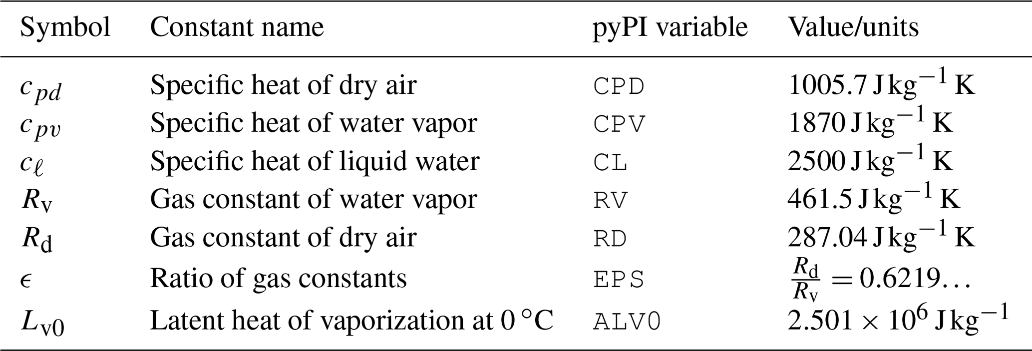
Constants used in to model potential intensity in the BE02 algorithm have been directly used in pyPI and are recorded in Table A1.
Table B1Python functions to compute or analyze the potential intensity algorithm.
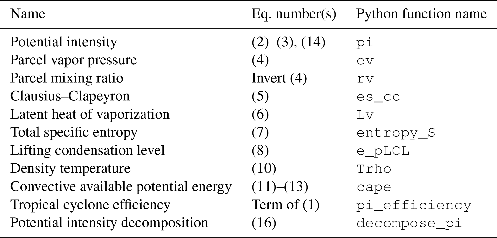
pyPI performs the calculations of Algorithms 1 and 2 through a set of functions included in the primary module or loaded from a utility file; these ensure consistency and enable modular changes to the codebase. Interested readers are encouraged to review the function list in Table B1 when considering a change to the pyPI codebase. Note that the CAPE and potential intensity modules include assumptions and internal calculations supporting Algorithms 1 and 2, which do not have their own Python functions. These are commented where they appear in the code and may be cross-referenced with the fully documented algorithm descriptions in Sects. 3.2 and 3.3.
pyPI version 1.3 and accompanying data for validation and sample analyses are available at https://github.com/dgilford/pyPI/releases/tag/v1.3 (last access: 26 April 2021) and archived at https://doi.org/10.5281/zenodo.3985975 (Gilford, 2020). pyPI is provided under the MIT license.
The author declares that there is no conflict of interest.
The code is made publicly available without any warranty, and permissions are provided pursuant to the MIT License (https://opensource.org/licenses/MIT, last access: 26 April 2021).
Thanks to the two anonymous reviewers, whose comments improved this study. The author is particularly grateful to Kerry Emanuel for his encouragement and permission to develop, document, and distribute pyPI and for his development of PI theory and the original PI algorithm. Thanks to Daniel Rothenberg for implementing a Numba optimization (Lam et al., 2015) of the primary pyPI module. Thanks to Allison Wing, Dan Chavas, Jonathan Lin, and Raphael Rousseau-Rizzi for helpful comments and suggestions on pyPI and its documentation.
This research has been supported by the National Science Foundation (grant no. ICER-1663807) and the National Aeronautics and Space Administration (grant no. 80NSSC17K0698).
This paper was edited by Paul Ullrich and reviewed by two anonymous referees.
Bell, M. M., Montgomery, M. T., and Emanuel, K. A.: Air–Sea Enthalpy and Momentum Exchange at Major Hurricane Wind Speeds Observed during CBLAST, J. Atmos. Sci., 69, 3197–3222, https://doi.org/10.1175/JAS-D-11-0276.1, 2012. a
Bister, M. and Emanuel, K. A.: Dissipative heating and hurricane intensity, Meteorol. Atmos. Phys., 65, 233–240, https://doi.org/10.1007/BF01030791, 1998. a, b, c, d
Bister, M. and Emanuel, K. A.: Low frequency variability of tropical cyclone potential intensity 1. Interannual to interdecadal variability, J. Geophys. Res.-Atmos., 107, 4801, https://doi.org/10.1029/2001JD000776, 2002. a, b, c, d, e, f, g, h, i, j, k
Blumberg, W. G., Halbert, K. T., Supinie, T. A., Marsh, P. T., Thompson, R. L., and Hart, J. A.: Sharppy: An open-source sounding analysis toolkit for the atmospheric sciences, B. Am. Meteorol. Soc., 98, 1625–1636, https://doi.org/10.1175/BAMS-D-15-00309.1, 2017. a, b
Bolton, D.: The Computation of Equivalent Potential Temperature, Mon. Weather Rev., 108, 1046–1053, https://doi.org/10.1175/1520-0493(1980)108<1046:TCOEPT>2.0.CO;2, 1980. a, b, c
Bryan, G. H.: Effects of surface exchange coefficients and turbulence length scales on the intensity and structure of numerically simulated hurricanes, Mon. Weather Rev., 140, 1125–1143, https://doi.org/10.1175/MWR-D-11-00231.1, 2012. a, b
Camargo, S., Sobel, A. H., Barnston, A. G., and Emanuel, K. A.: Tropical cyclone genesis potential index in climate models, Tellus A, 59, 428–443, https://doi.org/10.1111/j.1600-0870.2007.00238.x, 2007. a, b, c
Camargo, S. J.: Global and regional aspects of tropical cyclone activity in the CMIP5 models, J. Climate, 26, 9880–9902, https://doi.org/10.1175/JCLI-D-12-00549.1, 2013. a
Camargo, S. J. and Polvani, L. M.: Little evidence of a reduced global tropical cyclone activity following recent volcanic eruptions, npj Climate and Atmospheric Science, 2, 14, https://doi.org/10.1038/s41612-019-0070-z, 2019. a
Camargo, S. J., Wheeler, M. C., and Sobel, A. H.: Diagnosis of the MJO modulation of tropical cyclogenesis using an empirical index, J. Atmos. Sci., 66, 3061–3074, https://doi.org/10.1175/2009JAS3101.1, 2009. a
Chavas, D. R. and Emanuel, K.: Equilibrium tropical cyclone size in an idealized state of axisymmetric radiative-convective equilibrium, J. Atmos. Sci., 71, 1663–1680, https://doi.org/10.1175/JAS-D-13-0155.1, 2014. a
Dee, D. P., Uppala, S. M., Simmons, a. J., Berrisford, P., Poli, P., Kobayashi, S., Andrae, U., Balmaseda, M. a., Balsamo, G., Bauer, P., Bechtold, P., Beljaars, a. C. M., van de Berg, L., Bidlot, J., Bormann, N., Delsol, C., Dragani, R., Fuentes, M., Geer, a. J., Haimberger, L., Healy, S. B., Hersbach, H., Hólm, E. V., Isaksen, L., Kållberg, P., Köhler, M., Matricardi, M., McNally, a. P., Monge-Sanz, B. M., Morcrette, J.-J., Park, B.-K., Peubey, C., de Rosnay, P., Tavolato, C., Thépaut, J.-N., and Vitart, F.: The ERA-Interim reanalysis: configuration and performance of the data assimilation system, Q. J. Roy. Meteor. Soc., 137, 553–597, https://doi.org/10.1002/qj.828, 2011. a
Doswell, C. A. and Rasmussen, E. N.: The effect of neglecting the virtual temperature correction on CAPE calculations, Weather Forecast., 9, 625–629, https://doi.org/10.1175/1520-0434(1994)009<0625:TEONTV>2.0.CO;2, 1994. a
Elsner, J. B., Kossin, J. P., and Jagger, T. H.: The increasing intensity of the strongest tropical cyclones, Nature, 455, 92–95, https://doi.org/10.1038/nature07234, 2008. a
Emanuel, K.: A Statistical Analysis of Tropical Cyclone Intensity, Mon. Weather Rev., 128, 1139–1152, https://doi.org/10.1175/1520-0493(2000)128<1139:ASAOTC>2.0.CO;2, 2000. a, b, c, d, e
Emanuel, K.: Tropical Cyclones, Annu. Rev. Earth Pl. Sc., 31, 75–104, https://doi.org/10.1146/annurev.earth.31.100901.141259, 2003. a, b
Emanuel, K.: Hurricanes: Tempests in a greenhouse, Physics Today, 59, 74–75, https://doi.org/10.1063/1.2349743, 2006. a, b
Emanuel, K.: 100 Years of Progress in Tropical Cyclone Research, Meteor. Mon., 59, 15.1–15.68, https://doi.org/10.1175/AMSMONOGRAPHS-D-18-0016.1, 2018. a
Emanuel, K., DesAutels, C., Holloway, C., and Korty, R.: Environmental control of tropical cyclone intensity, J. Atmos. Sci., 61, 843–858, https://doi.org/10.1175/1520-0469(2004)061<0843:ECOTCI>2.0.CO;2, 2004. a, b
Emanuel, K., Solomon, S., Folini, D., Davis, S., and Cagnazzo, C.: Influence of Tropical Tropopause Layer Cooling on Atlantic Hurricane Activity, J. Climate, 26, 2288–2301, https://doi.org/10.1175/JCLI-D-12-00242.1, 2013. a, b
Emanuel, K. A.: An Air-Sea Interaction Theory for Tropical Cyclones. Part I: Steady-State Maintenance, J. Atmos. Sci., 43, 585–605, https://doi.org/10.1175/1520-0469(1986)043<0585:AASITF>2.0.CO;2, 1986. a, b
Emanuel, K. A.: The dependence of hurricane intensity on climate, Nature, 326, 483–485, https://doi.org/10.1038/326483a0, 1987. a, b, c, d
Emanuel, K. A.: Atmospheric Convection, Oxford University Press, 1994. a, b, c, d, e, f, g, h
Emanuel, K. A.: Sensitivity of tropical cyclones to surface exchange coefficients and revised steady-state model incorporating eye dynamics, J. Atmos. Sci., 52, 3969–3976, https://doi.org/10.1175/1520-0469(1995)052<3969:SOTCTS>2.0.CO;2, 1995. a, b, c
Emanuel, K. A.: Increasing destructiveness of tropical cyclones over the past 30 years, Nature, 436, 686–688, https://doi.org/10.1038/nature03906, 2005. a, b, c
Fueglistaler, S., Dessler, A. E., Dunkerton, T. J., Folkins, I., Fu, Q., and Mote, P. W.: Tropical tropopause layer, Rev. Geophys., 47, RG1004, https://doi.org/10.1029/2008RG000267, 2009. a, b
Garner, S.: The Relationship between Hurricane Potential Intensity and CAPE, J. Atmos. Sci., 72, 141–163, https://doi.org/10.1175/JAS-D-14-0008.1, 2015. a
Gelaro, R., McCarty, W., Suárez, M. J., Todling, R., Molod, A., Takacs, L., Randles, C. A., Darmenov, A., Bosilovich, M. G., Reichle, R., Wargan, K., Coy, L., Cullather, R., Draper, C., Akella, S., Buchard, V., Conaty, A., da Silva, A. M., Gu, W., Kim, G.-K., Koster, R., Lucchesi, R., Merkova, D., Nielsen, J. E., Partyka, G., Pawson, S., Putman, W., Rienecker, M., Schubert, S. D., Sienkiewicz, M., and Zhao, B.: The Modern-Era Retrospective Analysis for Research and Applications, Version 2 (MERRA-2), J. Climate, 30, 5419–5454, https://doi.org/10.1175/JCLI-D-16-0758.1, 2017. a
Gilford, D.: dgilford/pyPI: pyPI v1.3 (initial package release), https://doi.org/10.5281/zenodo.3985975, 2020. a
Gilford, D. M.: The Tropopause Region Thermal Structure and Tropical Cyclones, PhD thesis, Massachusetts Institute of Technology, available at: https://dspace.mit.edu/handle/1721.1/115639 (last access: 26 April 2021), 2018. a
Gilford, D. M., Solomon, S., and Emanuel, K. A.: On the Seasonal Cycles of Tropical Cyclone Potential Intensity, J. Climate, 30, 6085–6096, https://doi.org/10.1175/JCLI-D-16-0827.1, 2017. a, b, c, d, e, f, g, h
Gilford, D. M., Solomon, S., and Emanuel, K. A.: Seasonal Cycles of Along-Track Tropical Cyclone Maximum Intensity, Mon. Weather Rev., 147, 2417–2432, https://doi.org/10.1175/MWR-D-19-0021.1, 2019. a, b, c, d, e, f, g, h, i
Green, B. W. and Zhang, F.: Sensitivity of tropical cyclone simulations to parametric uncertainties in Air-Sea fluxes and implications for parameter estimation, Mon. Weather Rev., 142, 2290–2308, https://doi.org/10.1175/MWR-D-13-00208.1, 2014. a
Gualdi, S., Scoccimarro, E., and Navarra, A.: Changes in tropical cyclone activity due to global warming: Results from a high-resolution coupled general circulation model, J. Climate, 21, 5204–5228, https://doi.org/10.1175/2008JCLI1921.1, 2008. a
Holland, G. J.: The Maximum Potential Intensity of Tropical Cyclones, J. Atmos. Sci., 54, 2519–2541, https://doi.org/10.1175/1520-0469(1997)054<2519:TMPIOT>2.0.CO;2, 1997. a
Hsiang, S. M. and Jina, A. S.: The Causal Effect of Environmental Catastrophe on Long-Run Economic Growth: Evidence From 6,700 Cyclones, National Bureau of Economic Research Working Paper Series, 20352, 1–70, https://doi.org/10.3386/w20352, 2014. a
IPCC: Climate Change 2013: The Physical Science Basis. Contribution of Working Group I to the Fifth Assessment Report of the Intergovernmental Panel on Climate Change, Cambridge University Press, Cambridge, UK and New York, USA, https://doi.org/10.1017/CBO9781107415324, 2013. a
Kieu, C. and Wang, Q.: Stability of the tropical cyclone intensity equilibrium, J. Atmos. Sci., 74, 3591–3608, https://doi.org/10.1175/JAS-D-17-0028.1, 2017. a
Kieu, C. and Zhang, D.-L.: The Control of Environmental Stratification on the Hurricane Maximum Potential Intensity, Geophys. Res. Lett., 45, 6272–6280, https://doi.org/10.1029/2018GL078070, 2018. a
Kossin, J. P., Knapp, K. R., Olander, T. L., and Velden, C. S.: Global increase in major tropical cyclone exceedance probability over the past 40 years, P. Natl. Acad. Sci. USA, 117, 11975–11980, https://doi.org/10.1073/pnas.1920849117, 2020. a, b
Lam, S. K., Pitrou, A., and Seibert, S.: Numba: a LLVM-based Python JIT compiler, Proceedings of the Second Workshop on the LLVM Compiler Infrastructure in HPC – LLVM '15, Austin, TX, USA, 15–20 November 2015, 1–6, https://doi.org/10.1145/2833157.2833162, 2015. a, b
Lin, I.-I., Black, P., Price, J. F., Yang, C.-Y., Chen, S. S., Lien, C.-C., Harr, P., Chi, N.-H., Wu, C.-C., and D'Asaro, E. A.: An ocean coupling potential intensity index for tropical cyclones, Geophys. Res. Lett., 40, 1878–1882, https://doi.org/10.1002/grl.50091, 2013. a, b
Lin, N. and Emanuel, K.: Grey swan tropical cyclones, Nat. Clim. Change, 6, 106–111, https://doi.org/10.1038/nclimate2777, 2016. a
Manabe, S. and Strickler, R. F.: Thermal Equilibrium of the Atmosphere with a Convective Adjustment, J. Atmos. Sci., 21, 361–385, https://doi.org/10.1175/1520-0469(1964)021<0361:TEOTAW>2.0.CO;2, 1964. a
May, R. and Bruick, Z.: MetPy: An Community-Driven, Open-Source Python Toolkit for Meteorology, AGU Fall Meeting Abstracts, vol. 2019, pp. NS21A–16, 2019. a
McTaggart-Cowan, R., Deane, G. D., Bosart, L. F., Davis, C. A., and Galarneau, T. J.: Climatology of tropical cyclogenesis in the North Atlantic (1948-2004), Mon. Weather Rev., 136, 1284–1304, https://doi.org/10.1175/2007MWR2245.1, 2008. a
Millman, K. J. and Aivazis, M.: Python for Scientists and Engineers, Comput. Sci. Eng., 13, 9–12, 2011. a
Murnane, R. J. and Elsner, J. B.: Maximum wind speeds and US hurricane losses, Geophysical Research Letters, 39, 6–10, https://doi.org/10.1029/2012GL052740, 2012. a
Nystrom, R. G., Chen, X., Zhang, F., and Davis, C. A.: Nonlinear Impacts of Surface Exchange Coefficient Uncertainty on Tropical Cyclone Intensity and Air-Sea Interactions, Geophys. Res. Lett., 47, 1–10, https://doi.org/10.1029/2019GL085783, 2020. a
Pielke, R. A., Gratz, J., Landsea, C. W., Collins, D., Saunders, M. A., and Musulin, R.: Normalized hurricane damage in the United States: 1900–2005, Nat. Hazards Rev., 9, 29–42, https://doi.org/10.1061/(ASCE)1527-6988(2008)9:1(29), 2008. a
Polvani, L. M., Camargo, S. J., and Garcia, R. R.: The Importance of the Montreal Protocol in Mitigating the Potential Intensity of Tropical Cyclones, J. Climate, 29, 2275–2289, https://doi.org/10.1175/JCLI-D-15-0232.1, 2016. a, b
Powell, M. D.: Evaluations of Diagnostic Marine Boundary-Layer Models Applied to Hurricanes, Mon. Weather Rev., 108, 757–766, https://doi.org/10.1175/1520-0493(1980)108<0757:EODMBL>2.0.CO;2, 1980. a
Ramsay, H. A.: The Effects of Imposed Stratospheric Cooling on the Maximum Intensity of Tropical Cyclones in Axisymmetric Radiative–Convective Equilibrium, J. Climate, 26, 9977–9985, https://doi.org/10.1175/JCLI-D-13-00195.1, 2013. a, b
Randel, W. J. and Jensen, E. J.: Physical processes in the tropical tropopause layer and their roles in a changing climate, Nat. Geosci., 6, 169–176, https://doi.org/10.1038/NGEO1733, 2013. a
Randel, W. J. and Wu, F.: Variability of zonal mean tropical temperatures derived from a decade of GPS radio occultation data, J. Atmos. Sci., 72, 1261–1275, https://doi.org/10.1175/JAS-D-14-0216.1, 2014. a, b
Rappaport, E. N.: Fatalities in the united states from atlantic tropical cyclones: New data and interpretation, B. Am. Meteorol. Soc., 95, 341–346, https://doi.org/10.1175/BAMS-D-12-00074.1, 2014. a
Rashed, M. G. and Ahsan, R.: Python in Computational Science: Applications and Possibilities, Int. J. Comput. Appl., 46, 26–30, https://doi.org/10.5120/7058-9799, 2018. a
Romps, D. M.: Exact Expression for the Lifting Condensation Level, J. Atmos. Sci., 74, 3891–3900, https://doi.org/10.1175/JAS-D-17-0102.1, 2017. a, b
Rotunno, R. and Emanuel, K. A.: An Air–Sea Interaction Theory for Tropical Cyclones. Part II: Evolutionary Study Using a Nonhydrostatic Axisymmetric Numerical Model, J. Atmos. Sci., 44, 542–561, https://doi.org/10.1175/1520-0469(1987)044<0542:AAITFT>2.0.CO;2, 1987. a
Rousseau-Rizzi, R. and Emanuel, K.: An evaluation of hurricane superintensity in axisymmetric numerical models, J. Atmos. Sci., 76, 1697–1708, https://doi.org/10.1175/JAS-D-18-0238.1, 2019. a
Santer, B. D., Painter, J. F., Bonfils, C., Mears, C. A., Solomon, S., Wigley, T. M., Gleckler, P. J., Schmidt, G. A., Doutriaux, C., Gillett, N. P., Taylor, K. E., Thorne, P. W., and Wentz, F. J.: Human and natural influences on the changing thermal structure of the atmosphere, P. Natl. Acad. Sci. USA, 110, 17235–17240, https://doi.org/10.1073/pnas.1305332110, 2013. a
Shields, S., Gilford, D. M., and Wing, A.: A Global Analysis of Interannual Variability of Potential and Actual Tropical Cyclone Intensities, Geophys. Res. Lett., 47, e2020GL089512, https://doi.org/10.1029/2020GL089512, 2019. a, b, c, d, e
Sobel, A. H. and Camargo, S. J.: Projected Future Seasonal Changes in Tropical Summer Climate, J. Climate, 24, 473–487, https://doi.org/10.1175/2010JCLI3748.1, 2011. a
Sobel, A. H., Camargo, S. J., Hall, T. M., Lee, C.-y., Tippett, M. K., and Wing, A. A.: Human influence on tropical cyclone intensity, Science, 353, 242–246, 2016. a, b, c, d
Strazzo, S. E., Elsner, J. B., and LaRow, T. E.: Quantifying the sensitivity ofmaximum, limiting, and potential tropical cyclone intensity to SST: Observations versus the FSU/ COAPS global climate model, J. Adv. Model. Earth Syst., 7, 586–599, https://doi.org/10.1002/2015MS000432, 2015. a
Strazzo, S. E., Elsner, J. B., LaRow, T. E., Murakami, H., Wehner, M., and Zhao, M.: The influence of model resolution on the simulated sensitivity of North Atlantic tropical cyclone maximum intensity to sea surface temperature, J. Adv. Model. Earth Syst., 8, 1037–1054, https://doi.org/10.1002/2016MS000635, 2016. a
Tang, B. and Emanuel, K.: A ventilation index for tropical cyclones, B. Am. Meteorol. Soc., 93, 1901–1912, https://doi.org/10.1175/BAMS-D-11-00165.1, 2012. a, b
Tippett, M. K., Camargo, S. J., and Sobel, A. H.: A poisson regression index for tropical cyclone genesis and the role of large-scale vorticity in genesis, J. Climate, 24, 2335–2357, https://doi.org/10.1175/2010JCLI3811.1, 2011. a, b
Tonkin, H., Holland, G. J., Holbrook, N., and Henderson-Sellers, A.: An Evaluation of Thermodynamic Estimates of Climatological Maximum Potential Tropical Cyclone Intensity, Mon. Weather Rev., 128, 746–762, https://doi.org/10.1175/1520-0493(2000)128<0746:AEOTEO>2.0.CO;2, 2000. a
Tsuboki, K., Yoshioka, M. K., Shinoda, T., Kato, M., Kanada, S., and Kitoh, A.: Future increase of supertyphoon intensity associated with climate change, Geophys. Res. Lett., 42, 646–652, https://doi.org/10.1002/2014GL061793, 2015. a
Vecchi, G. A., Fueglistaler, S., Held, I. M., Knutson, T. R., and Zhao, M.: Impacts of atmospheric temperature trends on tropical cyclone activity, J. Climate, 26, 3877–3891, https://doi.org/10.1175/JCLI-D-12-00503.1, 2013. a
Vecchi, G. A., Delworth, T., Gudgel, R., Kapnick, S., Rosati, A., Wittenberg, A. T., Zeng, F., Anderson, W., Balaji, V., Dixon, K., Jia, L., Kim, H. S., Krishnamurthy, L., Msadek, R., Stern, W. F., Underwood, S. D., Villarini, G., Yang, X., and Zhang, S.: On the seasonal forecasting of regional tropical cyclone activity, J. Climate, 27, 7994–8016, https://doi.org/10.1175/JCLI-D-14-00158.1, 2014. a
Wallis, J.: A treatise of algebra, both historical and practical, printed by John Playford, https://doi.org/10.3931/E-RARA-8842, 1685. a
Wang, S., Camargo, S. J., Sobel, A. H., and Polvani, L. M.: Impact of the Tropopause Temperature on the Intensity of Tropical Cyclones: An Idealized Study Using a Mesoscale Model, J. Atmos. Sci., 71, 4333–4348, https://doi.org/10.1175/JAS-D-14-0029.1, 2014. a, b
Wehner, M. F., Reed, K. A., Loring, B., Stone, D., and Krishnan, H.: Changes in tropical cyclones under stabilized 1.5 and 2.0 ∘C global warming scenarios as simulated by the Community Atmospheric Model under the HAPPI protocols, Earth Syst. Dynam., 9, 187–195, https://doi.org/10.5194/esd-9-187-2018, 2018. a
Wing, A. A., Sobel, A. H., and Camargo, S. J.: Relationship between the potential and actual intensities of tropical cyclones on interannual time scales, Geophys. Res. Lett., 34, 1–5, https://doi.org/10.1029/2006GL028581, 2007. a, b, c, d, e
Wing, A. A., Emanuel, K., and Solomon, S.: On the factors affecting trends and variability in tropical cyclone potential intensity, Geophys. Res. Lett., 42, 8669–8677, https://doi.org/10.1002/2015GL066145, 2015. a, b, c, d, e, f, g
Xu, J., Wang, Y., and Yang, C.: Factors Affecting the Variability of Maximum Potential Intensity (MPI) of Tropical Cyclones Over the North Atlantic, J. Geophys. Res.-Atmos., 6654–6668, https://doi.org/10.1029/2019JD030283, 2019. a
Yulaeva, E., Holton, J. R., and Wallace, J. M.: On the Cause of the Annual Cycle in Tropical Lower-Stratospheric Temperatures, J. Atmos. Sci., 51, 169–174, https://doi.org/10.1175/1520-0469(1994)051<0169:OTCOTA>2.0.CO;2, 1994. a, b, c
Zhang, K., Randel, W. J., and Fu, R.: Relationships between outgoing longwave radiation and diabatic heating in reanalyses, Clim. Dynam., 49, 2911–2929, https://doi.org/10.1007/s00382-016-3501-0, 2016. a
online at http://wxmaps.org/pix/hurpot (last access: 26 April 2021)
Equation (4) in Bister and Emanuel (2002) mistakenly replaces Rd with cp. pyPI includes the correct factor of Rd.
This is likely derived empirically from Bolton (1980) and was developed for Emanuel (1994) (Kerry Emanuel, personal communication, 2020). Modern calculations of pLCL are made following exact expressions from Romps (2017); cf. Sect. 4.3.
When reduced by an order of magnitude to 0.05 hPa, Vmax values increase by <0.3 m s−1, while computation times increase by >25 %.
- Abstract
- Introduction
- Potential intensity theory
- The pyPI algorithm
- Python implementation
- Validation
- Example analyses
- Summary, limitations, and future development
- Appendix A: pyPI constants
- Appendix B: pyPI functions
- Code and data availability
- Competing interests
- Disclaimer
- Acknowledgements
- Financial support
- Review statement
- References