the Creative Commons Attribution 4.0 License.
the Creative Commons Attribution 4.0 License.
 | 06 Mar 2020
Beijing Climate Center Earth System Model version 1 (BCC-ESM1): model description and evaluation of aerosol simulations
Fang Zhang
Jie Zhang
Weihua Jie
Yanwu Zhang
Fanghua Wu
Laurent Li
Jinghui Yan
Xiaohong Liu
Haiyue Tan
Lin Zhang
The Beijing Climate Center Earth System Model version 1 (BCC-ESM1) is the first version of a fully coupled Earth system model with interactive atmospheric chemistry and aerosols developed by the Beijing Climate Center, China Meteorological Administration. Major aerosol species (including sulfate, organic carbon, black carbon, dust, and sea salt) and greenhouse gases are interactively simulated with a whole panoply of processes controlling emission, transport, gas-phase chemical reactions, secondary aerosol formation, gravitational settling, dry deposition, and wet scavenging by clouds and precipitation. Effects of aerosols on radiation, cloud, and precipitation are fully treated. The performance of BCC-ESM1 in simulating aerosols and their optical properties is comprehensively evaluated as required by the Aerosol Chemistry Model Intercomparison Project (AerChemMIP), covering the preindustrial mean state and time evolution from 1850 to 2014. The simulated aerosols from BCC-ESM1 are quite coherent with Coupled Model Intercomparison Project Phase 5 (CMIP5)-recommended data, in situ measurements from surface networks (such as IMPROVE in the US and EMEP in Europe), and aircraft observations. A comparison of modeled aerosol optical depth (AOD) at 550 nm with satellite observations retrieved from the Moderate Resolution Imaging Spectroradiometer (MODIS) and the Multi-angle Imaging SpectroRadiometer (MISR) and surface AOD observations from the AErosol RObotic NETwork (AERONET) shows reasonable agreement between simulated and observed AOD. However, BCC-ESM1 shows weaker upward transport of aerosols from the surface to the middle and upper troposphere, likely reflecting the deficiency of representing deep convective transport of chemical species in BCC-ESM1. With an overall good agreement between BCC-ESM1 simulated and observed aerosol properties, it demonstrates a success of the implementation of interactive aerosol and atmospheric chemistry in BCC-ESM1.
- Article
(16588 KB) - Full-text XML
- BibTeX
- EndNote


Atmosphere is a thin gaseous layer around the Earth, consisting of nitrogen, oxygen, and a large number of trace gases including important greenhouse gases (GHGs) such as water vapor, tropospheric ozone (O3), carbon dioxide (CO2), methane (CH4), nitrous oxide (N2O), and chlorofluorocarbons (CFCs). Besides gaseous components, atmosphere also contains various aerosols, which are important for cloud formation and radiative transfer. Atmospheric trace gases and aerosols are actually interactive components of the climate system. Their inclusion in global climate models (GCMs) is a significant enhancement for most state-of-the-art climate models (Lamarque et al., 2013; Collins et al., 2017). Early attempts at coupling global climate dynamics with atmospheric chemistry can be traced back to the late 1970s, when 3D transport of ozone and simple stratospheric chemistry were first incorporated into a GCM to simulate global O3 production and transport (e.g., Cunnold et al., 1975; Schlesinger and Mintz, 1979). Since the mid-1980s, a large number of online global climate–chemistry models have been developed to address issues of the Antarctic stratospheric O3 depletion (e.g., Cariolle et al., 1990; Austin et al., 1992; Solomon, 1999), tropospheric O3 and sulfur cycle (e.g., Feichter et al., 1996; Barth et al., 2000), tropospheric aerosol, and its interactions with cloud (e.g., Chuang et al., 1997; Lohmann et al., 2000; Ghan and Easter, 2006; Jacobson, 2012). Aerosols and chemically reactive gases in the atmosphere exert important influences on global and regional air quality and climate (Collins et al., 2017).
Since 2013, the Beijing Climate Center (BCC), China Meteorological Administration, has continuously developed and updated its fully coupled GCM, the Beijing Climate Center Climate System Model (BCC-CSM) (Wu et al., 2013, 2014, 2019). BCC-CSM version 1.1 was one of the comprehensive carbon–climate models participating in phase five of the Coupled Model Intercomparison Project (CMIP5; Taylor et al., 2012). When forced by prescribed historical emissions of CO2 from the combustion of fossil fuels and land-use change, BCC-CSM1.1 successfully reproduced the trends in observed atmospheric CO2 concentration and global surface air temperature from 1850 to 2005 (Wu et al., 2013). During recent years, BCC-CSM1.1 has been used in numerous investigations on soil organic carbon changes (e.g., Todd-Brown et al., 2014), ocean biogeochemistry changes (e.g., Mora et al., 2013), and carbon–climate feedbacks (e.g., Arora et al., 2013; Hoffman et al., 2014). BCC-CSM includes the main climate–carbon cycle processes (Wu et al., 2013), and the global mean atmospheric CO2 concentration is calculated from a prognostic equation of CO2 budget taking into account global anthropogenic CO2 emissions and interactive land–atmosphere and ocean–atmosphere CO2 exchanges.
In recent years, BCC has put large efforts into developing a global climate–chemistry–aerosol fully coupled Earth system model (the Beijing Climate Center Earth System Model version 1, BCC-ESM1) on the basis of BCC-CSM2 (Wu et al., 2019). The objective is to interactively simulate global aerosols (e.g., sulfate, black carbon) and the main greenhouse gases (e.g., O3, CH4, N2O, and CO2) in the atmosphere and to investigate feedbacks between climate and atmospheric chemistry. BCC-ESM1 is at the point of being publicly released, and it is actively used by BCC for several Coupled-Model Intercomparison Project 6 (CMIP6)-endorsed research initiatives (Eyring et al., 2016), including the Aerosol Chemistry Model Intercomparison Project (AerChemMIP; Collins et al., 2017) and the Coupled Climate–Carbon Cycle Model Intercomparison Project (C4MIP; Jones et al., 2016).
The purpose of this paper is to evaluate the performance of BCC-ESM1 in simulating aerosols and their optical properties in the 20th century. The description of BCC-ESM1 is presented in Sect. 2. The experimental protocol is given in Sect. 3. Section 4 presents the evaluations of aerosol simulations with comparisons to CMIP5-recommended data (Lamarque et al., 2010) and data obtained from both global surface networks and satellite observations. The regional and global characteristics compared to observations and estimates from other studies are analyzed. Simulations of aerosol optical properties in the 20th century are also analyzed in Sect. 4. Conclusions and discussions are summarized in Sect. 5. Information about code and data availability are found at the end of the paper.
Table 1Chemical species considered in BCC-AGCM3-Chem. Species marked with star (*) denote those added in BCC-ESM1 apart from the 63 species used in MOZART2. In the column of surface emission, interactive surface emissions are considered for sea salt and dust.

BCC-ESM1 is an Earth system model with interactive chemistry and aerosol components, in which the atmospheric component is the BCC Atmospheric General Model version 3 (Wu et al., 2019) with interactive atmospheric chemistry (hereafter BCC-AGCM3-Chem), the land component BCC Atmosphere and Vegetation Interaction Model version 2.0 (hereafter BCC-AVIM2.0), the ocean component Modular Ocean Model version 4 (MOM4)-L40, and sea ice component (sea ice simulator, SIS). Different components of BCC-ESM1 are fully coupled and interact with each other through fluxes of momentum, energy, water, carbon, and other tracers at their interfaces. The coupling between the atmosphere and the ocean is done every hour.
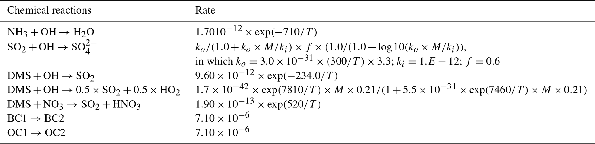
The atmospheric component BCC-AGCM3-Chem is able to simulate global atmospheric composition and aerosols from anthropogenic emissions as forcing agents. Its resolution is T42 (approximately transformed spectral grid). The model has 26 levels in a hybrid sigma–pressure vertical coordinate system with the top level at 2.914 hPa. Details of the model physics are described in Wu et al. (2019). The BCC-AGCM3-Chem combines 66 gas-phase chemical species and 13 bulk aerosol compounds as listed in Table 1. Apart from 3 gas-phase species of dimethyl sulfide (DMS), sulfur dioxide (SO2), and ammonia (NH3), the other 63 gas-phase species are the same as those in the “standard version” of MOZART2 (Model for Ozone and Related chemical Tracers, version 2), a global chemical transport model for the troposphere developed by the National Center for Atmospheric Research (NCAR) driven by meteorological fields from either climate models or assimilations of meteorological observations (Horowitz et al., 2003). Advection of all tracers in BCC-AGCM3-Chem is performed through a semi-Lagrangian scheme (Williamson and Rasch, 1989), and vertical diffusion within the boundary layer follows the parameterization of Holtslag and Boville (1993). The gas-phase chemistry of the 63 MOZART2 gas-phase species as listed in Table 1 is treated in the same way as that in the standard version of MOZART2 (Horowitz et al., 2003), and there are 33 photolytic reactions and 135 chemical reactions involving 30 dry deposited chemical species and 25 soluble gas-phase species. Dry-deposition velocities for the 15 trace gases including O3, carbon monoxide (CO), CH4, formaldehyde (CH2O), acetic acid (CH3OOH), hydrogen peroxide (H2O2), nitrogen dioxide (NO2), nitric acid (HNO3), polyacrylonitrile (PAN), acetone (CH3COCH3), peroxyacetic acid (CH3COOOH), acetaldehyde (CH3CHO), methylglyoxal (CH3COCHO), nitric oxide (NO), and pernitric acid (HNO4) are not computed interactively and are directly interpolated from MOZART2 climatological monthly mean deposition velocities (https://en.wikipedia.org/wiki/MOZART_(model), last access: 1 May 2014), which are calculated offline (Bey et al., 2001; Shindell et al., 2008) using a resistance-in-series scheme originally described in Wesely (1989). The dry-deposition velocities for the other 15 species including peroxy acetyl nitrate (PAN), methyl nitroacetate (ONIT), organic nitrates (ONITR), ethyl alcohol (C2H5OH), organic hydroxiperoxide (POOH), ethyl hydroperoxide (C2H5OOH), propylhydroperoxide (C3H7OOH), methylene glycol mono acetate (ROOH), glycolaldehyde (GLYALD), acetol (HYAC), methanol (CH3OH), propanoic acid (MACROOH), isoprene hydroxy hydroperoxide (ISOPOOH), carboxylic acid (XOOH), formaldehyde (HYDRALD), and hydrogen (H2) are calculated using prescribed deposition velocities of O3, CO, CH3CHO, or land surface type and surface temperature following the MOZART2 (Horowitz et al., 2003). Wet removal by in-cloud scavenging for 25 soluble gas-phase species in the standard version of MOZART2 uses the parameterization of Giorgi and Chameides (1985) based on their temperature-dependent effective Henry's law constants. In-cloud scavenging is proportional to the amount of cloud condensate converted to precipitation, and the loss rate depends on the amount of cloud water, the rate of precipitation formation, and the rate of tracer uptake by the liquid phase water. Other highly soluble species such as HNO3, H2O2, ONIT, ISOPOOH, MACROOH, XOOH, and lead (Pb-210) are also removed by below-cloud washout as calculated using the formulation of Brasseur et al. (1998). Below-cloud scavenging is proportional to the precipitation flux in each model layer and the loss rate depends on the precipitation rate. Vertical transport of gas tracers and aerosols due to deep convection is not yet included in the present version of BCC-AGCM3-Chem, a process which is regarded as a part of the deep convection and occurs generally in a small spatial region on a GCM box with a low resolution (2.8∘ lat. × 2.8∘ long.). Another consideration is that a large uncertainty exists in treating transport of those water-soluble tracers by deep convection. But this effect will be involved in the next version of BCC model.
The BCC-AVIM2.0 is the land model with a terrestrial carbon cycle. It is described in detail in Li et al. (2019) and includes biophysical, physiological, and soil carbon–nitrogen dynamical processes. The terrestrial carbon cycle operates through a series of biochemical and physiological processes on photosynthesis and respiration of vegetation. Biogenic emissions from vegetation are computed online in BCC-AVIM2.0 following the algorithm of the Model of Emissions of Gases and Aerosols from Nature version 2.1 (MEGAN2.1; Guenther et al., 2012).
The oceanic component of BCC-ESM1 is the Modular Ocean Model version 4 with 40 levels (hereafter MOM4-L40) and the sea ice component SIS. MOM4-L40 uses a tripolar grid of horizontal resolution with 1∘ longitude by 1∕3∘ latitude between 30∘ S and 30∘ N, 1∘ longitude by 1∘ latitude from 60∘ S and 60∘ N poleward, and 40 z levels in the vertical. Carbon exchange between the atmosphere and the ocean are calculated online in MOM4-L40 using a biogeochemistry module that is based on the protocols from the Ocean Carbon Cycle Model Intercomparison Project–Phase 2 (OCMIP2, http://www.ipsl.jussieu.fr/OCMIP/phase2/, last access: 1 August 2011). SIS has the same horizontal resolution as MOM4-L40 and three layers in the vertical, including one layer of snow cover and two layers of equally sized sea ice. Details of oceanic component MOM4-L40 and sea ice component SIS that are used in BCC-ESM1 may be found in Wu et al. (2013, 2019).
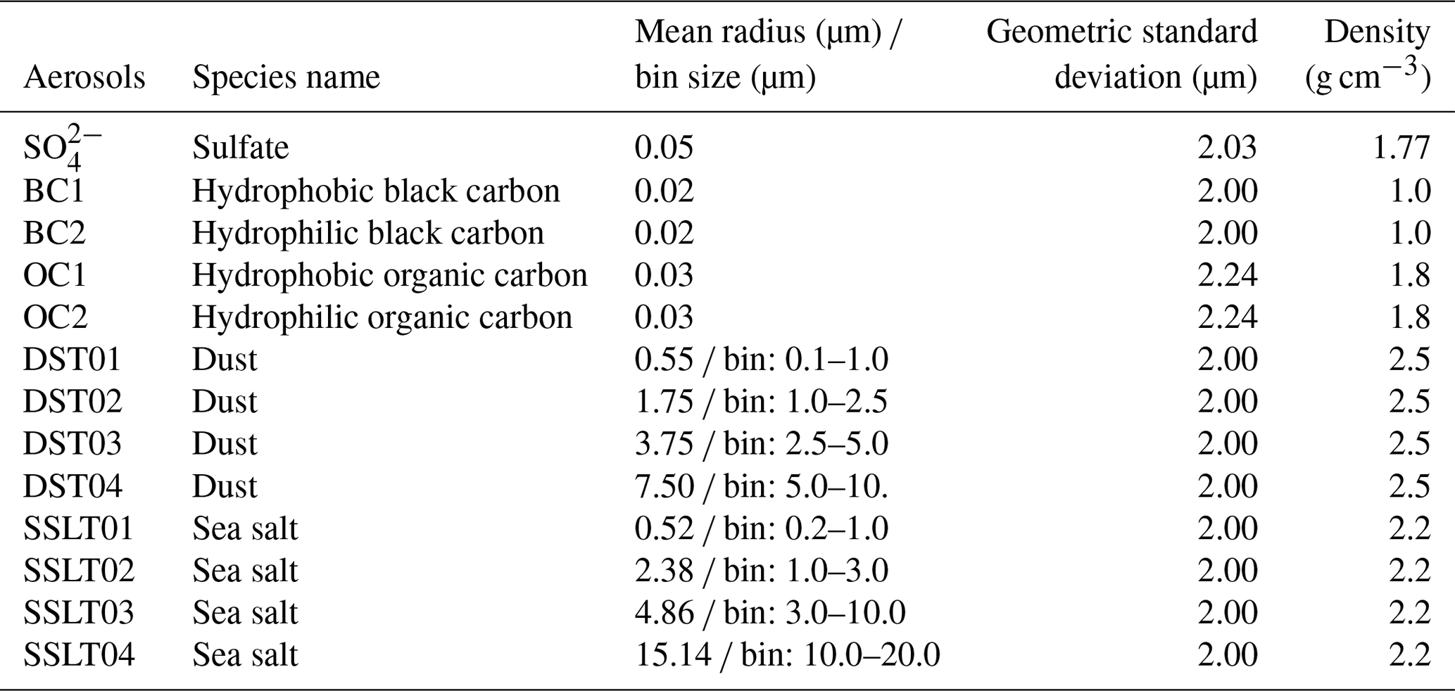
In the following subsections, we will describe the treatments in BCC-ESM1 for 3 gas-phase species of DMS, SO2 and NH3, 13 prognostic aerosol species including sulfate (), 2 types of organic carbon (hydrophobic OC1, hydrophilic OC2), 2 types of black carbon (hydrophobic BC1, hydrophilic BC2), 4 categories of soil dust (DST01, DST02, DST03, DST04), and 4 categories of sea salt (SSLT01, SSLT02, SSLT03, SSLT04). Concentrations of all aerosols in BCC-ESM1 are mainly determined by advective transport, emission, dry deposition, gravitational settling, and wet scavenging by clouds and precipitation, except for , the gas-phase and aqueous-phase conversion of which from SO2 are also considered. The present version of aerosol scheme belongs to a bulk aerosol model and mainly refers to the scheme of CAM-Chem (Lamarque et al., 2012), but the nucleation and coagulation of aerosols are still ignored.
Table 2Gas-phase chemical reactions for NH3 and bulk aerosols precursors following CAM-Chem (Lamarque et al., 2012). The reaction rates (s−1) refer to Tie et al. (2001) and Sander et al. (2003) and Cooke and Wilson (1996). Temperature (T) is expressed in kelvin, air density (M) in molecule per cubic centimeter, and ki and ko in cubic centimeters per molecule per second.
2.1 SO2, DMS, NH3, and sulfate
SO2 is a main sulfuric acid precursor to form aerosol sulfate . Conversions of SO2 to occur by gas-phase reactions (Table 2) and by aqueous-phase reactions in cloud droplets. The dry-deposition velocity of SO2 follows the resistance-in-series approach of Wesely (1989) using the formula , in which ra, rb, and rc are the aerodynamic resistance, the quasi-laminar boundary layer resistance, and the surface resistance, respectively and they are interactively computed in each model time step. The loss rate of SO2 due to wet deposition is computed following the scheme in the global Community Atmosphere Model (CAM) version 4, the atmospheric component of the Community Earth System Model (Lamarque et al., 2012).
The sources of SO2 mainly come from fuel combustion, industrial activities, and volcanoes. SO2 can also be formed from the oxidation of DMS as listed in Table 2, in which their reaction rates follow CAM-Chem (Lamarque et al., 2012). The main source of DMS is from oceanic emissions via biogenic processes. It is prescribed with the climatological monthly data that are extracted from the MOZART2 package (https://www2.acom.ucar.edu/gcm/mozart-4, last access: 10 February 2018). is one of the prognostic aerosols in BCC-AGCM3-Chem. Its treatment follows CAM4-Chem (Lamarque et al., 2012). It is produced primarily by the gas-phase oxidation of SO2 (in Table 2) and by aqueous-phase oxidation of SO2 in cloud droplets. The gas-phase reactions, rate constants, and gas–aqueous equilibrium constants are given by Tie et al. (2001). The heterogeneous reactions of occur on all aerosol surfaces. Their treatment follows a bulk aerosol model (BAM) used in CAM4 (Neale et al., 2010). The heterogeneous reactions depend strongly on pH values in clouds, which are calculated from the concentrations of SO2, HNO3, H2O2, NH3, O3, HO2, and . NH3 is a gas tracer apart from MOZART2 (Table 1). Its sources include aircraft and surface emissions due to anthropogenic activity, biomass burning, and biogenic emissions from land soil and ocean surfaces (Table 4). is assumed to be all in aqueous phase due to water uptake, although Wang et al. (2008a) showed that ∼ 34 % of sulfate particles are in solid phase globally due to the hysteresis effect of ammonium sulfate phase transition. However, in terms of radiative forcing, consideration of the solid sulfate formation process lowers the sulfate forcing by ∼ 8 % as compared to a consideration of all sulfate particles in the aqueous phase (Wang et al., 2008b). Future model development may consider the life cycle of NH3. The sulfate in- and below-cloud scavenging follows Neu and Prather (2011). Washout of is set to 20 % of the washout rate of HNO3 following Tie et al. (2005) and Horowitz (2006). The dry-deposition velocity of is also calculated by the resistance-in-series approach.
2.2 Aerosols of organic carbon and black carbon
BCC-AGCM3-Chem treats two types of organic carbon (OC), i.e., water-insoluble tracer OC1 and water-soluble tracer OC2, and two types of black carbon (BC), i.e., water-insoluble tracer BC1 and water-soluble tracer BC2. As shown in Table 2, hydrophobic BC1 and OC1 can be converted to hydrophilic BC2 and OC2 with a constant rate of s−1 (Cooke and Wilson, 1996). The four tracers of organic carbon and black carbon are mainly from emissions including both fossil fuel and biomass burning and are from the CMIP6 data package (https://esgf-node.llnl.gov/search/input4mips/, last access: 10 March 2019; Hoesly et al., 2018). Beside anthropogenic and biomass burning emissions, hydrophilic organic carbon OC2 can also come from natural biogenic volatile organic compound (VOC) emissions. Dry-deposition velocities for all the four OC and BC tracers are set to 0.001 m s−1. OC2 and BC2 are soluble aerosols, and their sinks are primarily governed by wet deposition. Their in- and below-cloud scavenging follows the scheme of Neu and Prather (2011).
2.3 Sea salt aerosols
As shown in Table 3, sea salt aerosols in the model are classified into four size bins (0.2–1.0, 1.0–3.0, 3.0–10, and 10–20 µm) in diameter. They originate from oceans and are calculated online by BCC-ESM1. The upward flux Fsea-salt of sea salt productions for four bins is proportional to the 3.41 power of the wind speed u10 m at 10 m height near the sea surface (Mahowald et al., 2006) and is expressed as
where S is a scaling factor and set to , , , and for four size bins of sea salt aerosols in BCC-ESM1, respectively.
Dry deposition of sea salt depends on the turbulent deposition velocity in the lowest atmospheric layer using aerodynamic resistance and the friction velocity and the settling velocity through the whole atmospheric column for each bin of sea salt. The turbulent deposition velocity and settling velocity depend on particle diameter and density (listed in Table 3). In addition, the fact that the size of sea salt changes with humidity is also considered. The wet deposition of sea salt follows the scheme for soluble aerosols used in CAM4 and depends on prescribed solubility and size-independent scavenging coefficients.
2.4 Dust aerosols
Dust aerosols behave in a similar way to sea salt. Their variations involve three major processes: emission, advective transport, and wet or dry depositions. The dust emission is based on a saltation–sandblasting process and depends on wind friction velocity, soil moisture, and vegetation or snow cover (Zender et al., 2003). The vertical flux of dust emission is corrected by a surface erodible factor at each model grid cell which has been downloaded from the NCAR website (https://svn-ccsm-inputdata.cgd.ucar.edu/trunk/inputdata/atm/cam/dst/, last access: 1 May 2014). Soil erodibility is prescribed by a physically based geomorphic index that is proportional to the runoff area upstream of each source region (Albani et al., 2014). Like sea salt, dry deposition of dust aerosols includes gravitational and turbulent deposition processes, while wet deposition results from both convective and large-scale precipitation and is dependent on prescribed size-independent scavenging coefficients.
2.5 Effects of aerosols on radiation, clouds, and precipitation
The mass mixing ratios of bulk aerosols are prognostic variables in BCC-ESM1 and directly affect the radiative transfer in the atmosphere with their treatments following the NCAR Community Atmosphere Model (CAM3; Collins et al., 2004). Indirect effects of aerosols are taken into account in the present version of BCC-AGCM3-Chem (Wu et al., 2019). Aerosol particles act as cloud condensation nuclei and exert influence on cloud properties and precipitation and ultimately impact the hydrological cycle. Prognostic aerosol masses are used to estimate the liquid cloud droplet number concentration Ncdnc (cm−3) in BCC-AGCM3-Chem. Ncdnc is explicitly calculated using the empirical function suggested by Boucher and Lohmann (1995) and Quaas et al. (2006):
where maero (µg m−3) is the total mass of all hydrophilic aerosols,
i.e., the first bin of sea salt (mSS), hydrophilic organic carbon (mOC), sulfate (), and ammonium nitrite (NH4NO2). A dataset of NH4NO2 from NCAR CAM-Chem (Lamarque et al., 2012) is used in our model.
Ncdnc is an important factor in determining the effective radius of cloud droplets for radiative calculation. The effective radius of cloud droplets rel is estimated as
where β is a parameter dependent on the droplets' spectral shape and follows the calculation proposed by Peng and Lohmann (2003):
rl,vol is the volume-weighted mean cloud droplet radius:
where ρw is the liquid water density and LWC the cloud liquid water content (g cm−3).
Aerosols also exert impacts on precipitation efficiency (Albrecht, 1989), which is taken into account in the parameterization of non-convective cloud processes. There are five processes that convert condensate to precipitate: auto-conversion of liquid water to rain, collection of cloud water by rain, auto-conversion of ice to snow, collection of ice by snow, and collection of liquid by snow. The auto-conversion of cloud liquid water to rain (PWAUT) is dependent on the cloud droplet number concentration and follows a formula that was originally suggested by Chen and Cotton (1987):
where is the in-cloud liquid water mixing ratio, ρa and ρw are the local densities of air and water, respectively, and Cl,aut is a constant. H(x) is the Heaviside step function with the definition
rlc,vol is the critical value of mean volume radius of liquid cloud droplets rl,vol and is set to 15 µm.
The treatment of aerosol single-scattering (optical) properties (such as mass extinction efficiency, single-scattering albedo, and asymmetric factor) follows the lookup table approach in CAM (Collins et al., 2004). The optics for black and organic carbon, sea salt, and sea salt particles is assumed to be the same as the optics for soot and water-soluble aerosols in the Optical Properties of Aerosols and Clouds (OPAC) dataset (Hess et al., 1998). The optics for dust are derived by Mie calculations for the size distribution represented by each size bin (Zender et al., 2003). Similarly, for sulfate and nitrate particles, the same set of aerosol optical properties for ammonium sulfate is used and is taken from Wang et al. (2008b) with a treatment of aerosol hygroscopicity. The volcanic stratospheric aerosols are assumed to be comprised of 75 % sulfuric acid and 25 % water, as in Hess et al. (1998). For each model year, different aerosol types are assumed to be externally mixed in the calculation of bulk aerosol single-scattering properties that are in turn used in the radiative transfer calculations.
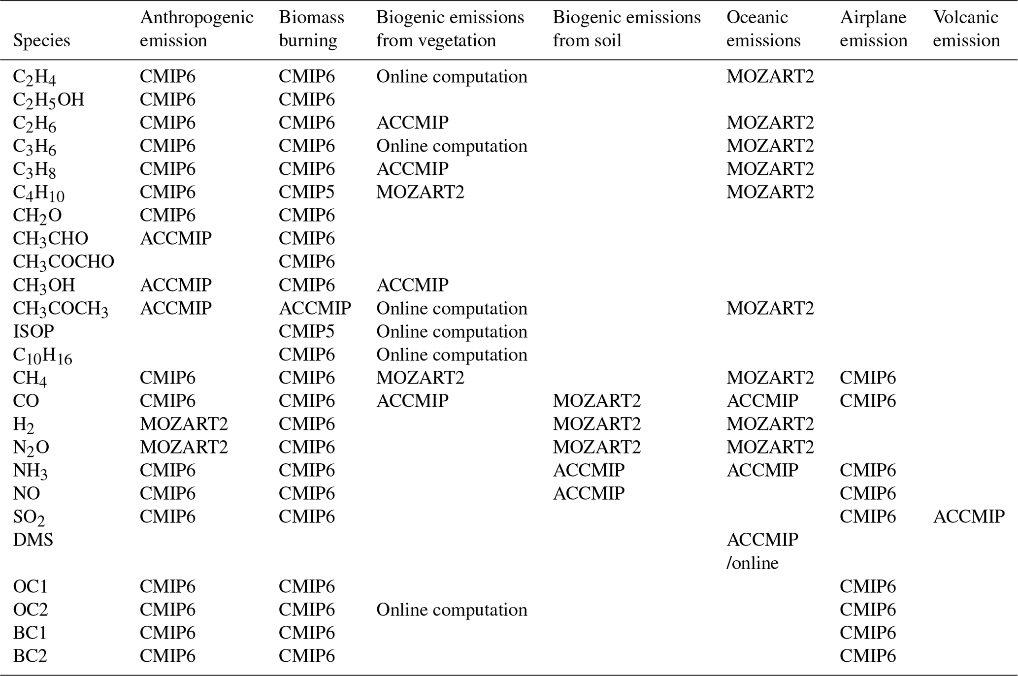
Table 4Sources of emission data. MOZART2 data denote the standard tropospheric chemistry package for MOZART and contain surface emissions from the EDGAR 2.0 database (Olivier et al., 1996). ACCMIP data are downloaded from the IPCC ACCMIP emission inventory (http://accent.aero.jussieu.fr/ACCMIP.php, last access: 1 May 2014) and they vary from 1850 to 2000, in 10-year steps (Lamarque et al., 2010). CMIP6 data are from https://esgf-node.llnl.gov/search/input4mips/ (last access: 10 March 2019). Anthropogenic emission includes industrial and fossil fuel use, agriculture, ships, etc. Biomass burning includes vegetation fires, such as fuel wood and agricultural burning.
AerChemMIP (Collins et al., 2017) is endorsed by CMIP6 for documenting and understanding past and future changes in the chemical composition of the atmosphere and estimating the global-to-regional climate response from these changes. Modeling groups with full chemistry and aerosol models are encouraged to perform all AerChemMIP simulations (Collins et al., 2017). To assess the ability of our model to simulate aerosols (mean and variability), we have followed the historical simulation designed by CMIP6 (Eyring et al., 2016) which is called the “historical” experiment in the Earth System Grid Federation (ESGF). The historical experiment is forced with emissions evolving from 1850 to 2014 that include biomass burning emissions (Van Marle et al., 2017) and anthropogenic and open burning emissions (Hoesly et al., 2018; Feng et al., 2019). O3 in the historical simulation is an interactive prognostic variable and feeds back on radiation, and the concentrations of other well-mixed greenhouse gases (WMGHGs), e.g., CH4, N2O, CO2, CFC11, and CFC12, are prescribed using CMIP6 historical forcing data (Meinshausen et al., 2017). Although CH4 and N2O are prognostic variables in the chemistry scheme (Table 1), their prognostic values at each model step in the historical experiment are replaced by CMIP6 data (Meinshausen et al., 2017) throughout the model domain. The rest of the historical forcing data include (1) yearly global gridded land-use forcing datasets (Hurtt et al., 2011, 2017) and (2) solar forcing (Matthes et al., 2017). All these datasets were downloaded from https://esgf-node.llnl.gov/search/input4mips/ (last access: 10 March 2019). Climate feedback processes that involve changes to the atmospheric composition of reactive gases and aerosols may affect the temperature response to a given WMGHG concentration level.
3.1 Surface emissions
Surface emissions of chemical species from different sources are summarized in Table 4. They include anthropogenic emissions from fossil fuel burning and other industrial activities, biomass burning (including vegetation fires, fuel wood, and agricultural burning), biogenic emissions from vegetation and soils, and oceanic emissions. Most historical emissions from anthropogenic sources (surface, aircraft plus ship) and biomass burning from 1850 to 2014 are CMIP6-recommended data (available at https://esgf-node.llnl.gov/search/input4mips (last access: 10 March 2019). Anthropogenic or biomass burning sources of some tracers which are not included in the CMIP6 dataset (see Table 4), and anthropogenic emission of H2 and N2O are from the monthly climatological dataset provided by the MOZART-2 standard package. N2O is a prognostic variable in BCC-ESM1, but it is replaced by CMIP6 prescribed concentration in the historical run. Other emissions including biomass burning (CH3COCH3) and anthropogenic emission (CH3CHO, CH3OH, and CH3COCH3) are from the Atmospheric Chemistry and Climate Model Intercomparison Project (ACCMIP) emission inventory (http://accent.aero.jussieu.fr/ACCMIP.php, last access: 1 May 2014) covering the period from 1850 to 2010 with 10-year intervals (see Table 4). Monthly lumped emissions of black carbon and organic carbon aerosols from 1850 to 2014 are downloaded from CMIP6-recommended data, but we used 80 % (for BC) and 50 % (for OC) of them in their hydrophobic forms (BC1 and OC1) and the rest in their hydrophilic forms (BC2 and OC2), following the work of Chin et al. (2002).
Five tracers of isoprene (C3H8O; ISOP), acetone (CH3COCH3), C2H4, C3H8, and monoterpenes (C10H16) in Table 1 belong to biogenic VOCs. As shown in Table 4, those VOC emissions are calculated online in BCC-ESM1 following the modeling framework of MEGAN2.1 (Guenther et al., 2012) using simple mechanistic algorithms to account for major known processes controlling biogenic emissions. MEGAN2.1 can provide a flexible scheme for estimating 16 tracers of biogenic emissions from terrestrial ecosystems including five VOC emissions used in BCC-ESM1 (Table 4). All the VOC emissions depend on current and past surface air temperature, solar flux, and the landscape types. Their calculation requires global maps of plant functional type (PFT) and leaf area index (LAI), which is a prognostic variable from the land model BCC-AVIM2. The effect of atmospheric CO2 concentration on isoprene emissions is included. Overall, 10 % of the biogenic monoterpene emissions as calculated online with the MEGAN2.1 algorithm in BCC-AVIM2 is converted to hydrophilic organic carbon (OC2) to account for the formation of secondary organic aerosols following Chin et al. (2002) in this version of BCC-ESM1.
3.2 Volcanic eruptions, lightning, and aircraft emissions
As there is no stratospheric aerosol scheme in BCC-ESM1, concentrations of sulfate aerosol at heights from 5 to 39.5 km, which are of volcanic origin, are directly prescribed using the CMIP6-recommended data (Thomason et al., 2018) from 1850 to 2014. The effects of surface SO2 emissions from volcanic eruption on the variation in SO2 in the atmosphere and then on the variation in tropospheric concentration are considered, and the SO2 emissions from 1850 to 2014 are downloaded from the IPCC ACCMIP emission inventory (http://accent.aero.jussieu.fr/ACCMIP.php, last access: 1 May 2014). Aircraft emissions are provided for NO2, CO, CH4, NH3, NO, SO2, and aerosols of OC and BC (Table 1). The emissions of NO from lightning are calculated online in BCC-AGCM3-Chem following the parameterization in MOZART2, and the globally averaged mean during the period of 1850 to 2014 is 5.19 Tg (N) yr−1, which is in agreement with observations within the range of 3 to 6 Tg (N) yr−1 (Martin et al., 2002). The lightning frequency depends strongly on the convective cloud top height, and the ratio of cloud-to-cloud versus cloud-to-ground lightning depends on the cold cloud thickness from the level of 0∘ to the cloud top (Price and Rind, 1992).

Figure 1The time series of global and annual mean of (a) net energy budget at the top of the atmosphere (W m−2), (b) near-surface air temperature (K), and (c) sea surface temperature (K) in the last 450 years of the piControl simulation.
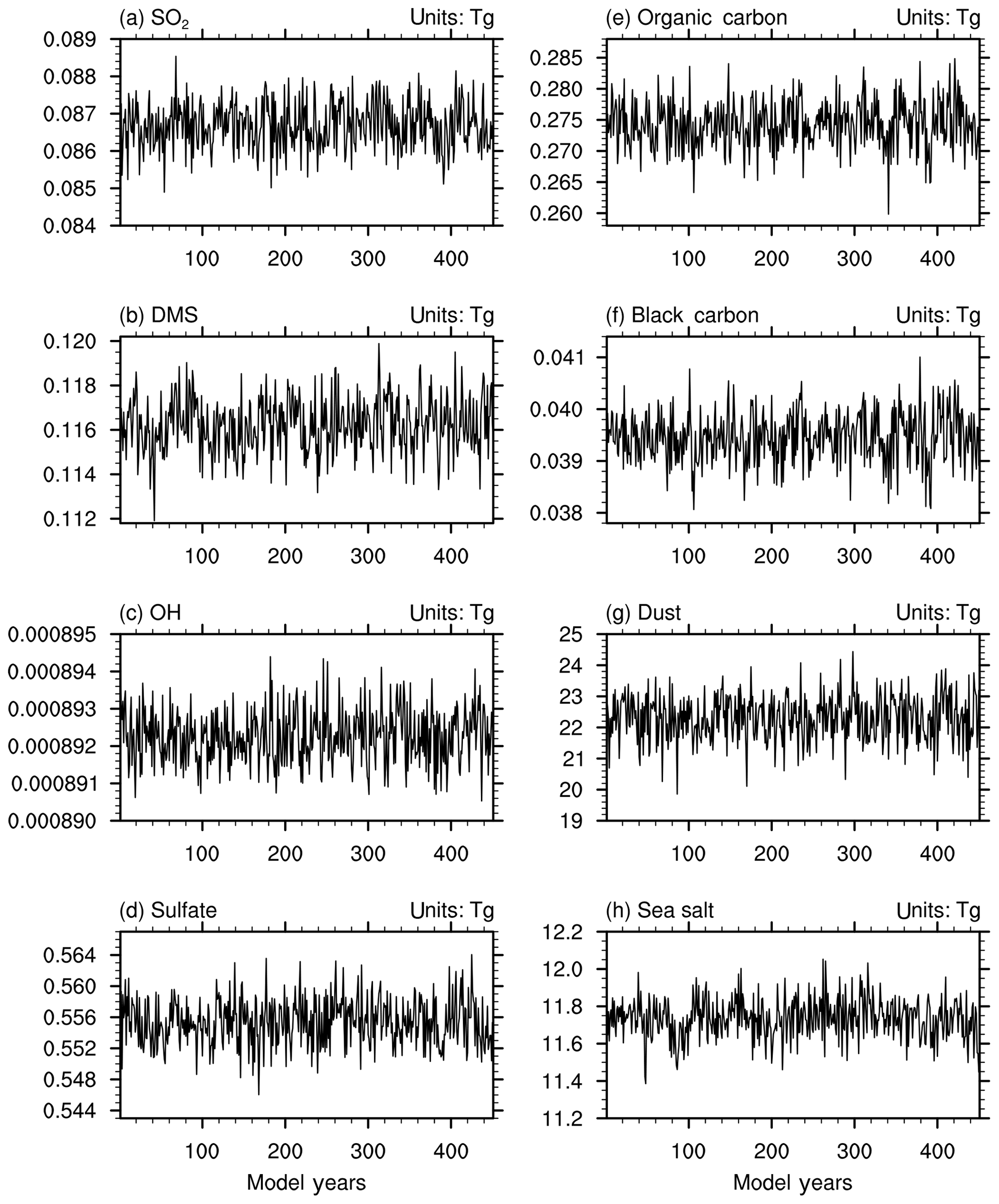
Figure 2Same as in Fig. 1, but for the global burdens of (a) SO2, (b) DMS, (c) OH, and (d–h) different aerosols in the troposphere (below 100 hPa). Units are teragrams.
3.3 Upper boundary of the atmosphere
As no stratospheric chemistry is included in the present version of BCC-AGCM3-Chem, it is necessary to ensure a proper distribution of chemically active stratospheric species. Concentrations of different tracers (O3, CH4, N2O, NO, NO2, HNO3, CO, and N2O5) at the top two layers of the model are set to prescribed monthly climatological values, and concentrations from below the top two layers to the tropopause are relaxed at a relaxation time of 10 d towards the climatology. Climatological values of NO, NO2, HNO3, CO, and N2O5 at the top two layers are extracted from the MOZART2 data package available at the website (https://www2.acom.ucar.edu/gcm/mozart-4, last access: 1 February 2018), originating from the Study of Transport and Chemical Reactions in the Stratosphere (STARS; Brasseur et al., 1997). Concentrations for the other tracers (O3, CH4, and N2O) at the top two model layers are the zonally averaged and monthly values from 1850 to 2014 derived from the CMIP6 data package.
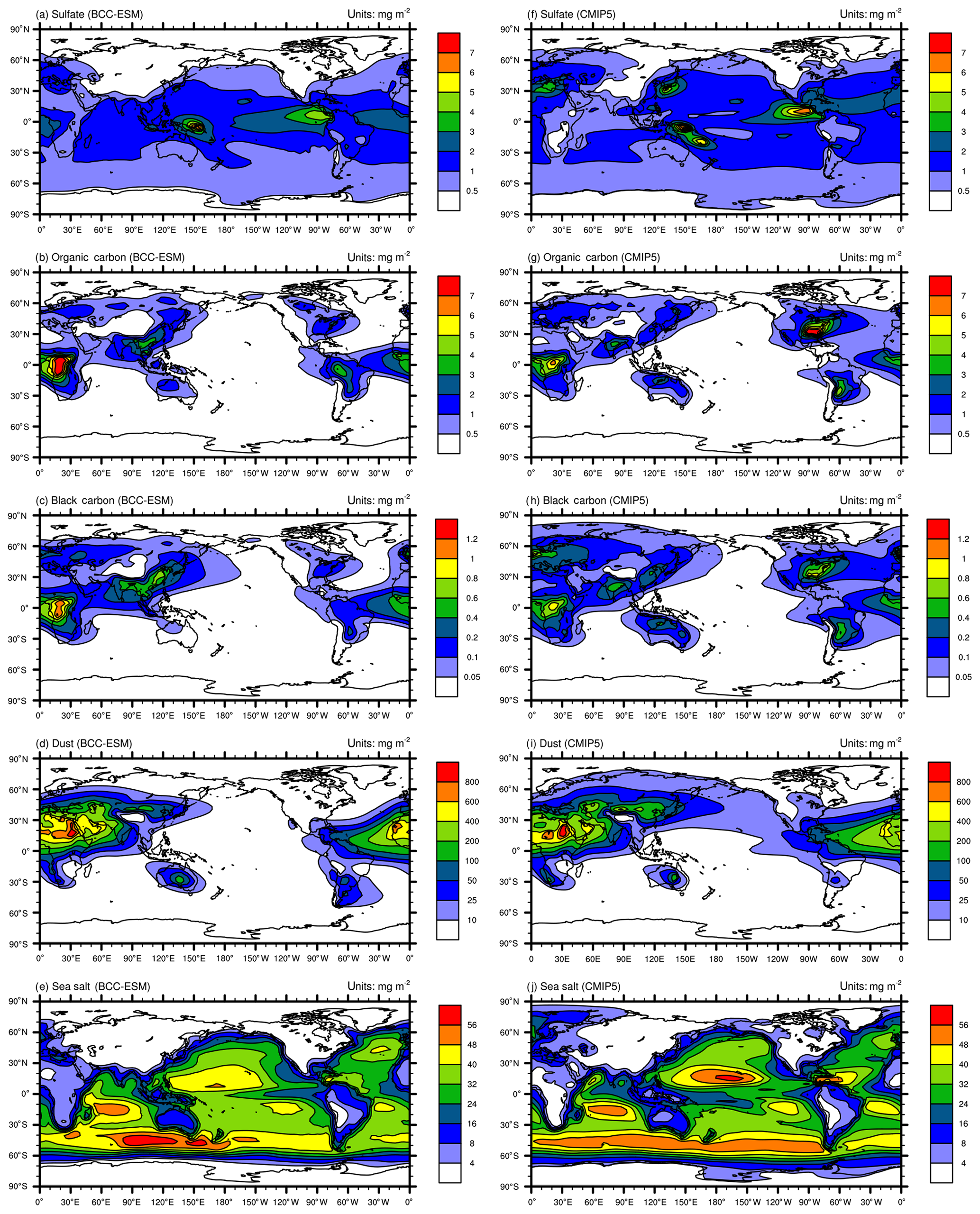
Figure 3Global distributions of annual mean mass burdens of sulfate (; a, f), organic carbon (OC; b, g), black carbon (BC; c, h), dust (d, i), and sea salt (e, j) aerosols in the whole atmospheric column. Panels (a–e) show the mean averaged for the last 100 years of BCC-ESM preindustrial piControl simulations, and (f–j) show the CMIP5 recommended aerosol concentrations in the year 1850 (the website at IIASA http://tntcat.iiasa.ac.at/RcpDb/, last access: 10 January 2012). Units: milligram per square meter.
3.4 The preindustrial model states
The preindustrial state of BCC-ESM1 is obtained from a piControl simulation of over 600 years in which all forcings including emissions data are fixed at 1850 conditions. The initial state of the piControl simulation itself is obtained through individual spin-up runs of each component of BCC-ESM1 in order for the piControl simulation to run stably and fast to reach its equilibrium. Figure 1a–c show the time series of global yearly means of the net energy budget at the top of the atmosphere (TOA), near-surface air temperature (TAS), and sea surface temperature (SST) from the piControl simulation for the last 450 years. It shows that the surface climate in BCC-ESM1 nearly reaches its equilibrium after 600 years of piControl simulation. The whole system in BCC-ESM1 fluctuates around +0.7 W m−2 net energy flux at TOA without an obvious trend in 450 years (Fig. 1a). This level of TOA energy imbalance is close to the average imbalance (1.0 W m−2) among CMIP5 models (Wild et al., 2013). It means that there exists a surplus energy of +0.7 W m−2 obtained by the whole system in BCC-ESM1, but this does not cause remarkable climate drift. The global mean TAS and SST stay around 288.1 K (Fig. 1b) and 295.05 K (Fig. 1c), respectively. During the last 450 years, there are (±0.2 K amplitude of TAS and SST) oscillations of centennial scale for the whole globe (Fig. 1b and c), which are certainly caused by internal variation in the system.
Figure 2a–c show the time series of global annual total burdens of SO2, DMS, and OH in the troposphere (integrated from the surface to 100 hPa) in the last 450 years of the piControl simulation. Without any anthropogenic source, the SO2 amount in the troposphere stays almost at the level of 0.0868 Tg in the 450 years of the piControl simulation. Tropospheric DMS varies around the value of 0.116 Tg. Tropospheric OH, as an important gas species oxidizing SO2 to form (Table 2), keeps at a stable level in the atmosphere. also remains at a stable level of 0.556 Tg in the atmosphere in the whole period of the piControl simulation (Fig. 2d). The amounts of BC and OC in the troposphere vary around 0.0395 Tg and 0.275 Tg (Fig. 2e–f), respectively. Dust and sea salt aerosols are at the level of 22 Tg and 11.7 Tg (Fig. 2g–h), respectively. All those data are close to the global mean concentrations of 0.604 Tg , 0.046 Tg BC, 0.30 Tg OC, 22.18 Tg dust, and 11.73 Tg sea salt in 1850, which are estimated based on the CMIP5 prescribed data in 1850 (Lamarque et al., 2010).
Figure 3 shows the global spatial distributions of annual mean sulfate, organic carbon, black carbon, dust, and sea salt aerosols in the whole atmospheric column averaged for the last 100 years of the piControl simulation of BCC-ESM. We can compare them with CMIP5 recommended concentrations in the year 1850, regarded as the reference state at the preindustrial stage. At that time, there are fewer anthropogenic or biomass SO2 emissions; the over land is evidently smaller than that over oceans, especially over the tropical Pacific and Atlantic oceans, where DMS can be oxidized to SO2 and then form . There are several centers of high values of black carbon and organic carbon in East and South Asia, Europe, southeast America, and in the tropical rain forests in Africa and South America. They mainly result from biomass burning including vegetation fires, fuel wood, and agricultural burning. Dust aerosols are mainly distributed in North Africa, Central Asia, North China, and Australia, where arid and semiarid areas are located. Dust emitted from the Sahara can be transported to the tropical Atlantic by easterly wind. The sea salt aerosols are mainly distributed over the midlatitude southern oceans, the tropical southern Indian Ocean, and the tropical northern Pacific Ocean, where wind speeds near the sea surface are strong. As shown in Fig. 3, all the spatial distribution patterns of CMIP5-derived sulfate, black carbon, organic carbon, dust, and sea salt aerosols (Lamarque et al., 2010) are well simulated in BCC-ESM1. There are high spatial correlation coefficients (0.76 for sulfate, 0.77 for black carbon, 0.77 for organic carbon, 0.94 for dust, and 0.94 for sea salt) between CMIP5 data and BCC-ESM1 simulations. Relatively lower relations for sulfate, black carbon, and organic carbon are possibly due to different anthropogenic emission sources being used in BCC-ESM1 and to create CMIP5 data. Dust and sea salt belong to natural aerosols and depend on the land and sea surface conditions, so their spatial distributions are easy to capture and have relatively higher correlations between CMIP5 data and BCC-ESM1 simulations.
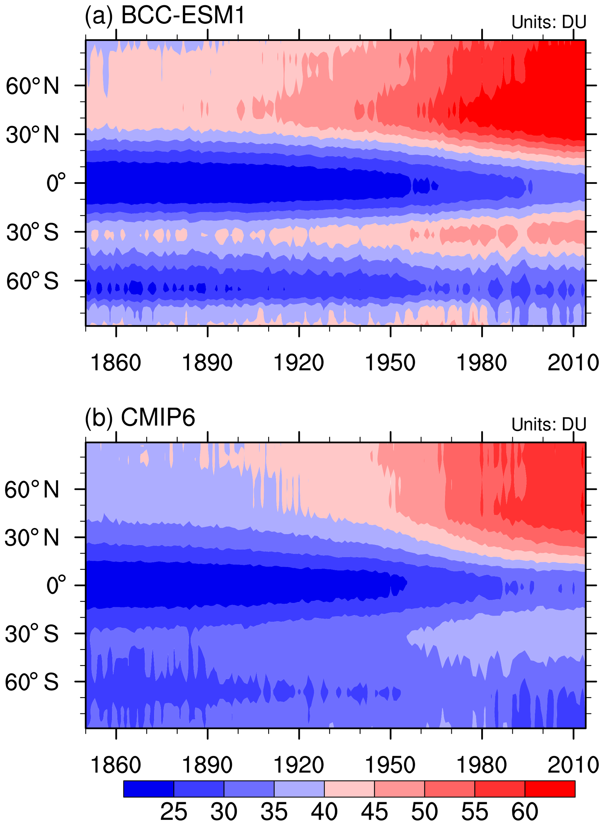
Figure 4Zonal mean of the yearly mean concentration of the ozone column in the troposphere below 300 hPa to the ground from 1871 to 1999 for (a) BCC-ESM1 and (b) CMIP6 data. Unit: DU.
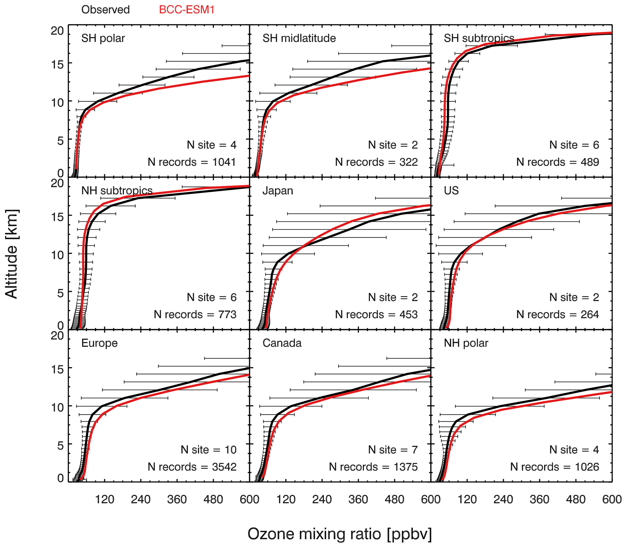
Figure 5Vertical profiles of annual mean ozone concentrations from observations averaged for 2010–2014 in nine regions (black) and from the BCC-ESM1 simulations (red). The observations are derived from 41 global WOUDC sites.
The rate of sulfate formation is dependent on the levels of oxidants in the troposphere. O3 is an important oxidant. So, the evaluation of simulated tropospheric O3 is helpful to understand the aerosol simulations. BCC-ESM1 is driven by most of the CMIP6-recommended emission data. As shown in Fig. 4, the zonal distributions of the total amounts of tropospheric O3 below 300 hPa to the ground and their changes with time from 1850 to 2014 from the CMIP6-recommend dataset (Table 4) are well simulated by BCC-ESM1. Evident increasing trends since 1850 exist at almost every latitude, especially in the Northern Hemisphere where the contents of tropospheric O3 are higher than in the Southern Hemisphere.
Figure 5 shows the vertical profiles of O3 simulations with a comparison to global ozonesonde observations averaged for the monthly data over 2010–2014 from the World Ozone and Ultraviolet Radiation Data Centre (WOUDC; http://woudc.org/data.php, last access: 24 September 2019) in nine regions, which are averaged from 41 global WOUDC sites. The details of WOUDC data may be found in Lu et al. (2019). As shown in Fig. 5, BCC-ESM1 captures the observed ozone vertical structure well in all regions. In the lower and middle troposphere (i.e., below 6 km), the model typically shows positive bias within 5 ppbv for the Southern Hemisphere and 10 ppbv for the northern midlatitudes, similar to those simulated by many other global atmospheric chemical models (Young et al., 2013, 2018). The model has larger ozone overestimation in the upper troposphere and stratosphere in most regions, at least partly due to the use of prescribed stratospheric ozone as upper boundary conditions and/or errors in modeling ozone exchange between the stratosphere and the troposphere. The global tropospheric ozone burden derived from our simulation is 335 Tg averaged over 2010–2014, consistent with a recent assessment from multi chemistry models (Young et al., 2018).

Figure 6Global annual anthropogenic, natural, and total emissions of SO2, organic carbon (OC), and black carbon (BC) in the BCC-ESM1 historical simulation. All the biomass burning emissions are included in natural emissions in (a–c). Units: teragrams per year.
4.1 Global aerosol trends
Figure 6a–c show the time series of global total emissions of SO2, OC, and BC to the atmosphere from natural and anthropogenic sources. Emissions of SO2 are largely due to industrial production. From 1850 to 1915, SO2 emissions increased year by year as the industrial revolution intensified and expanded. But from 1915 to 1945, the increased trend in SO2 emissions became slower as the First and the Second World Wars broke out. After that period, with growing industrial production, SO2 emissions increased again and reached a maximum around the end of 1970s. With a substantial decrease in SO2 emissions in Europe and the United States, the global SO2 emissions has been decreasing since the 1980s despite the rapid increase in SO2 emissions in South and East Asia as well as in developing countries in the Southern Hemisphere in recent years (Liu et al., 2009). The OC and BC emissions have substantially increased since the 1950s just after the Second World War. The global total OC emission in 2010 was nearly twice as high as that in the preindustrial period (before the year 1850) and increased by 18 Tg yr−1. Anthropogenic black carbon emissions increased from 1 Tg yr−1 in 1850 to nearly 8 Tg yr−1 in 2010.
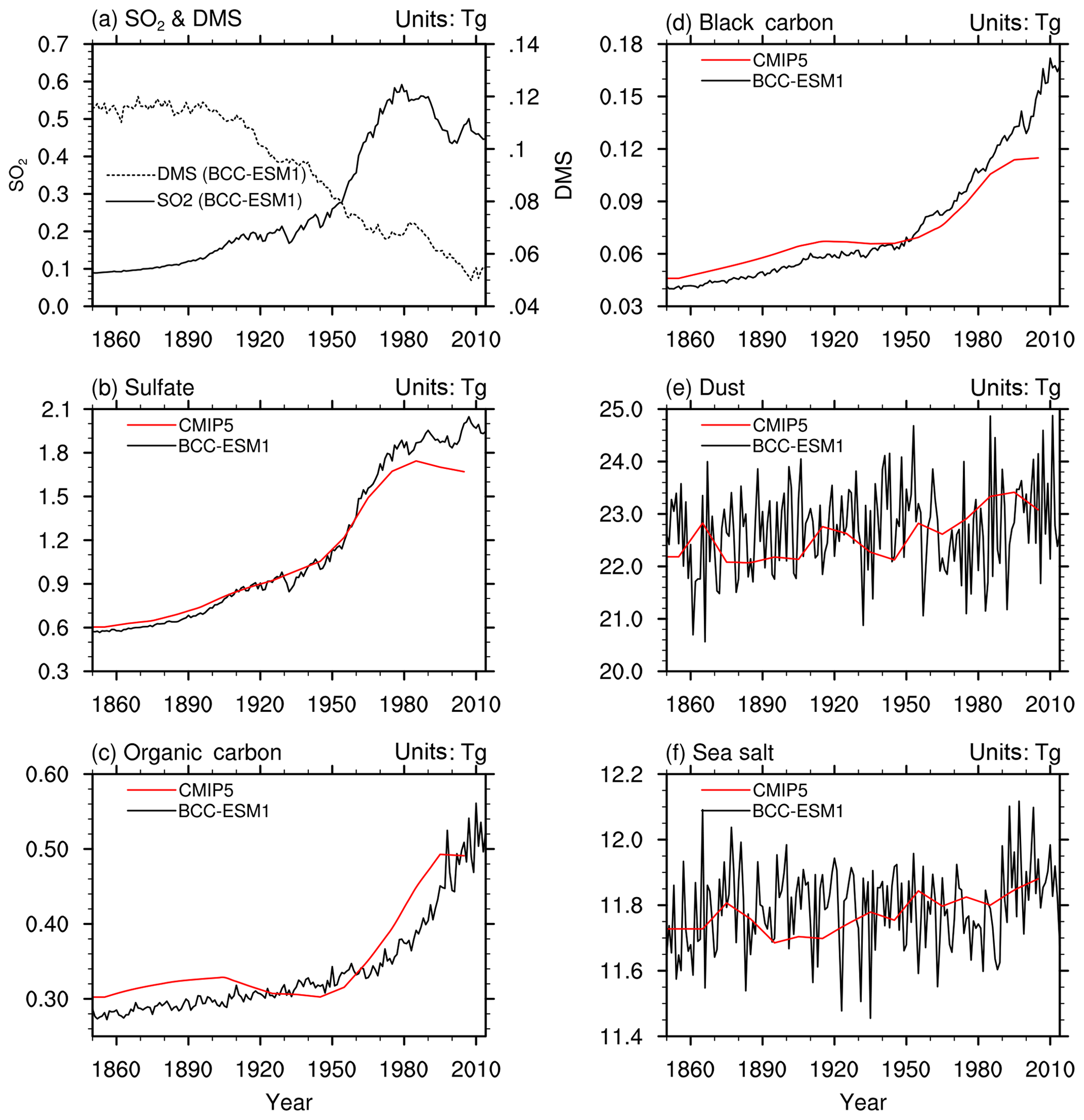
Figure 7The time series of global yearly amounts of (a) SO2 and DMS and (b–f) aerosols in the whole atmosphere column from the CMIP6 historical simulations of BCC-ESM1 (black lines) and the CMIP5-recommended aerosol masses (red lines). The yearly CMIP5 data are interpolated from the time series at a 10-year interval. Units: teragrams.
Anthropogenic SO2, OC, and BC emissions strongly affect the variations in atmospheric concentrations of sulfate, OC, and BC. The global gridded data of CMIP5-recommended aerosol masses with a 10-year interval from 1850 to 2000 (Lamarque et al., 2010) provides an important reference to evaluate the aerosol simulations in BCC-ESM1. As shown in Fig. 7b–f, the annual total aerosol burdens of , OC, and BC in the whole atmosphere column as simulated by the BCC-ESM1 20th-century historical simulation are generally consistent with the values derived from CMIP5-recommended aerosols concentrations. Due to increasing SO2 emissions from 1850 to the present day (Fig. 6), the global SO2 burden in the atmosphere increased from 100 Tg in the 1850s to 200 Tg in the 1980s (Fig. 7a) and has a high correlation coefficient of 0.996 with the anthropogenic emissions (Fig. 6a), as the lifetime of SO2 is short. The burden directly followed the emission. DMS in the atmosphere is oxidized by OH and NO3 to form SO2 (Table 2). Its natural emissions from oceans from 1850 to 2010 in the model are the climatological monthly means (Dentener et al., 2006) from MOZART2 data package. As shown in Fig. 7a, the global amount of DMS in the whole atmosphere was about 0.12 Tg during 1850–1900 and decreased to 0.055 Tg in 2010. This decrease trend maybe partly results from the speeded rate of DMS oxidation with global warming, and the loss of DMS gradually exceeds the source of ocean DMS emission to cause a net loss of DMS in the atmosphere since the 1910s. Largely driven by SO2 anthropogenic emissions, the sulfate burden shows three different stages from 1850 to the present. In the first period from the 1850s to the 1900s, the sulfate burden had a weak linear increase. It increased significantly in the second stage from the 1910s to the 1940s and then exploded from the 1950s until the middle 1970s and early 1980s. The sulfate burden then remained nearly stable and even showed slight decreases as seen from the CMIP5 data. As for global BC and OC burdens, BCC-ESM1 results have shown continuous increases since the 1850s, especially from 1950 to the present. From the 1910s to the 1940s, the CMIP5 data showed a slight decrease in BC and OC burdens in the atmosphere.
The dust and sea salt aerosols in the atmosphere are largely determined by the atmospheric circulations and states of the land and ocean surface. We can see that the global dust burden in the atmosphere showed an evident increase from 1980 to 2000, which could be partly caused by evident global warming since 1980 and increasing soil dryness resulting in more surface dust to be released into the atmosphere. Their details will be explored in second part.
4.2 Global aerosol budgets
We further evaluate global aerosol budgets by comparing a 10-year average of BCC-ESM results from 1990 to 2000 with various studies for sulfate, BC, OC, sea salt, and dust. Their annual total emissions, average atmospheric mass loading, and mean lifetimes are listed in Tables 5 and 6. It is worth emphasizing that the global mean total source and sink for each type of aerosols in BCC-ESM1 are almost balanced.
Table 5Global budgets for DMS, SO2, and sulfate in the period of 1991 to 2000. Units for sources and sinks: teragrams (S) per year; for burden: teragrams; for lifetime: days.
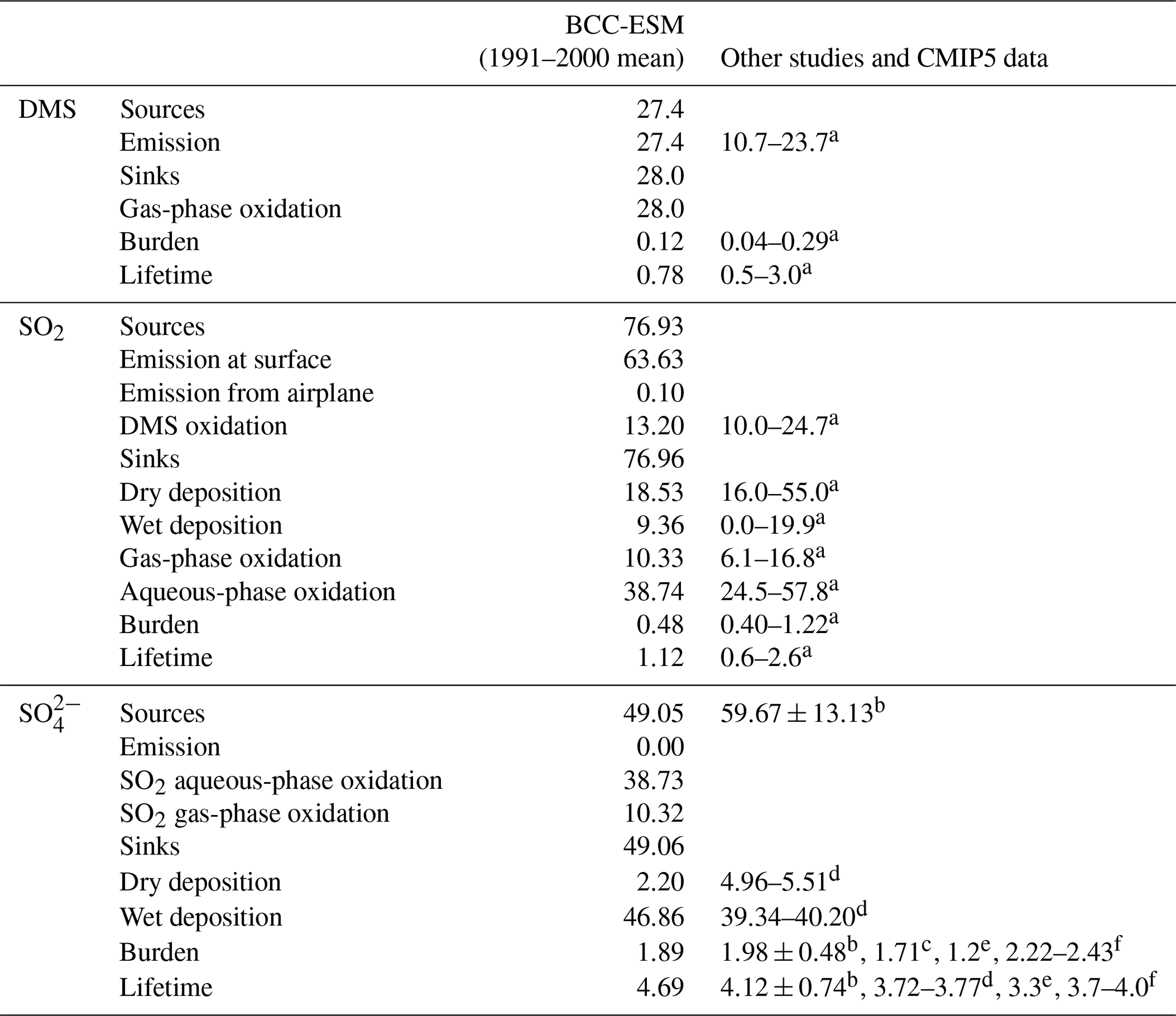
a Liu et al. (2005). b Textor et al. (2006). c Values derived from CMIP5 prescribed aerosol masses averaged from 1991 to 2000. d Liu et al. (2012). e Matsui and Mahowald (2017). f Tegen et al. (2019). Values of DMS, SO2, and sulfate burdens from dLiu et al. (2012) are transferred from teragrams S to teragrams (species) for unit consistency.
The global DMS emission from the ocean is 27.4 Tg (S) yr−1 in BCC-ESM. This emission in BCC-ESM is nearly balanced by the gas-phase oxidation of DMS to form SO2. The DMS burden is 0.12 Tg with a lifetime of 0.78 d, which is within the range of other models reported in the literature. As shown in Table 5, the total SO2 production averaged for the period of 1991 to 2000 is 76.93 Tg (S) yr−1. A rate of 13.2 Tg (S) yr−1 (about 17 %) SO2 is produced from the DMS oxidation; only 0.1 Tg (S) yr−1 SO2 is from airplane emissions to the atmosphere, and the rest (63.63 Tg (S) yr−1, almost 82.7 %) is from anthropogenic activities and volcanic eruption at the surface. The amount of SO2 produced from the DMS oxidation is in the range of other works (10.0 to 24.7 Tg (S) yr−1) reported in Liu et al. (2005). All the SO2 production is balanced by SO2 losses by dry and wet deposition and by gas- and aqueous-phase oxidation. Half of its loss (38.74 Tg (S) yr−1) occurs via its aqueous-phase oxidation to form sulfate. Other losses through dry and wet depositions and gas-phase oxidation to form are also important (Table 2). All the sinks are in the range from the literature (Liu et al., 2005). The global burden of SO2 in the atmosphere is 0.48 Tg with a lifetime of 1.12 d, consistent with values in literature (Liu et al., 2005).
Sulfate aerosol is mainly produced from aqueous-phase SO2 oxidation (38.73 Tg (S) yr−1) and partly from gaseous-phase oxidation of SO2 (10.32 Tg (S) yr−1) and is largely lost by wet scavenging (49.06 Tg (S) yr−1). The total production in BCC-ESM is at the lower range of values in other models reported in Textor et al. (2006). Its global burden is 1.89 Tg and the lifetime is 4.69 d, which is within the range of 1.71 to 2.43 Tg and 3.3 to 5.4 d in the literature (Textor et al., 2006; Liu et al., 2012, 2016; Matsui and Mahowald, 2017; Tegen et al., 2019; the value is derived from CMIP5 data).
Sources of BC and OC are mainly from anthropogenic emissions. Based on the CMIP6 data, there are, on average, 7.22 Tg yr−1 BC and 13.91 Tg yr−1 OC from fossil and bio-fuel emissions and 18.38 Tg yr−1 OC from natural emission during the period of 1991 to 2000. Most of these are scavenged through convective and large-scale rainfall processes. The rest returns to the surface by dry deposition. The simulated global BC and OC burdens are 0.13 and 0.62 Tg, respectively (Table 6), all close to the values of 0.114 Tg BC and 0.69 Tg OC derived from the CMIP5 data and within the range of 0.11–0.26 Tg BC (Textor et al., 2006; Matsui and Mahowald, 2017; Tegen et al., 2019) and less than the values of 1.25–2.2 Tg OC in other literature (Textor et al., 2006; Tegen et al., 2019). The simulated BC and OC lifetimes are 6.6 and 5.0 d, respectively, and are close to the recent values of 5.0–7.5 d BC and 5.4–6.6 d OC in the literature (Matsui and Mahowald, 2017; Tegen et al., 2019).
Table 6Same as Table 5, but for global budgets for black carbon, organic carbon, dust, and sea salt. Units for sources and sinks: teragrams per year; for burden: teragrams; for lifetime: days.
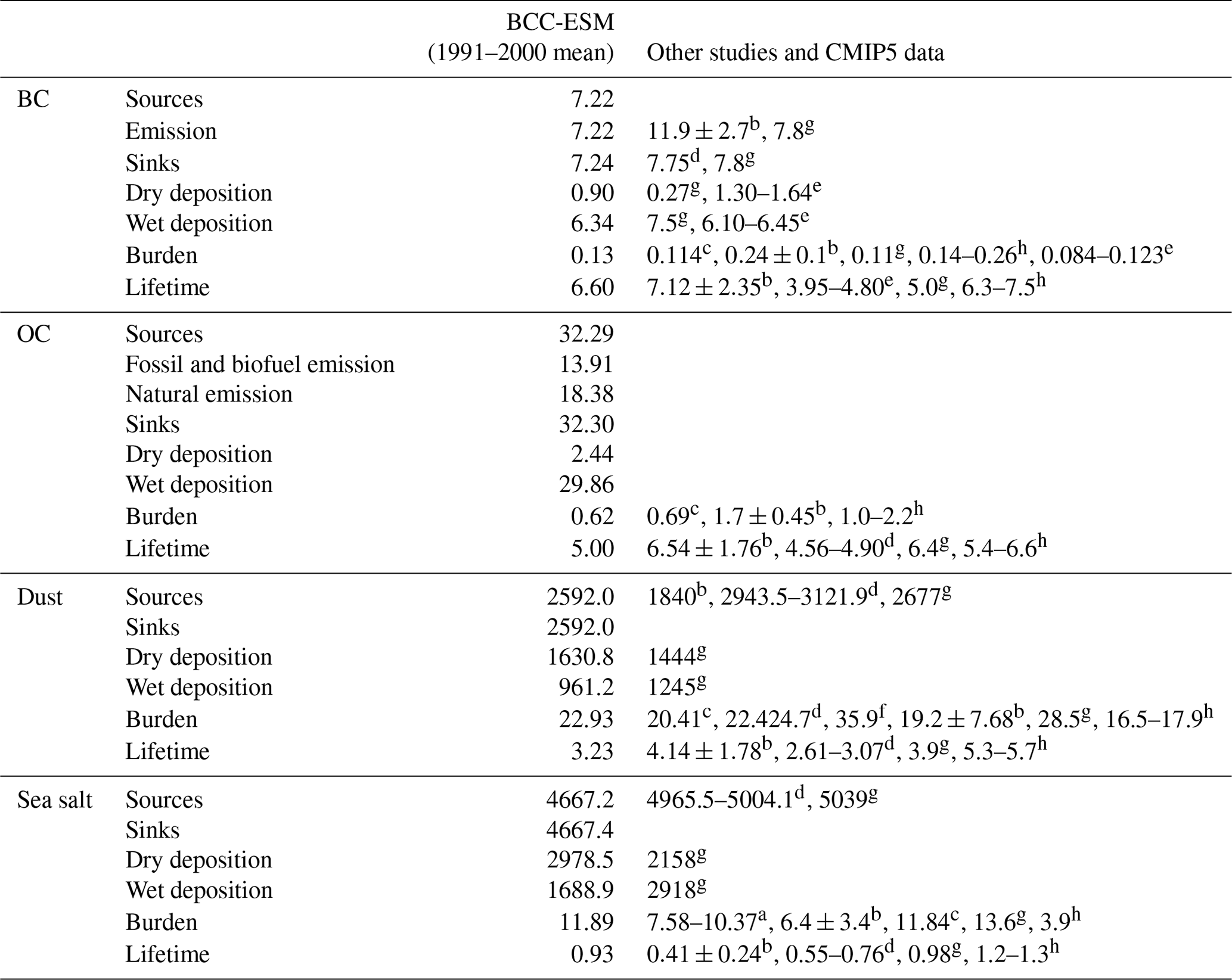
Notes: References denote a for Liu et al. (2005), b for Textor et al. (2006), c derived from CMIP5 prescribed aerosol masses averaged from 1991 to 2000, d for Liu et al. (2012), e for Liu et al. (2016), f for Ginoux et al. (2001), g for Matsui and Mahowald (2017), and h for Tegen et al. (2019).
The emissions of dust and sea salt are mainly determined by winds near the surface. The annual total dust emission in BCC-ESM1 is 2592 Tg yr−1, higher than the AeroCom multi-model mean (1840 Tg yr−1; Textor et al., 2006) but comparable to other studies (Chin et al., 2002; Liu et al., 2012; Matsui and Mahowald, 2017). The average dust loading is 22.93 Tg, lower than the value of 35.9 Tg in Ginoux et al. (2001) but slightly higher than the value of 20.41 Tg derived from CMIP5 data. The average lifetime for dust particles is 3.23 d, which is shorter than the AeroCom mean (4.14 d) and the value of 3.9 d in a recent study (Matsui and Mahowald, 2017). The simulated sea salt emission is 4667.2 Tg yr−1, slightly lower than the simulated value in Liu et al. (2012) and substantially lower than the AeroCom mean (16 600 Tg yr−1; Textor et al., 2006). The simulated sea salt burdens are 11.89 Tg and close to the CMIP5 data. Their averaged lifetimes are 0.93 d and close to the value in the recent of Matsui and Mahowald (2017) but longer than the AeroCom mean (0.41 d; Textor et al., 2006).
4.3 Global aerosol distributions in the present day
Figures 8–12 show December–January–February (DJF) and June–July–August (JJA) mean column mass concentrations of sulfate (), OC, BC, dust, and sea salt aerosols averaged for the period of 1991–2000. Here, BCC-ESM1 simulated results are compared with the CMIP5-recommended data for the same period. Unlike the preindustrial level of sulfate shown in Fig. 2, sulfate concentrations in the present day (Fig. 8) are strongly influenced by anthropogenic emissions and have maximum concentrations in the industrial regions (e.g., East Asia, Europe, and North America). Their seasonal variations are distinct and are characterized by high concentrations in boreal summer and low concentrations in boreal winter. These spatial distributions simulated by BCC-ESM1 show good consistency with the CMIP5 data, with spatial correlation coefficients in DJF and JJA reaching 0.92 and 0.83 (Fig. 13), respectively. In DJF, the deviation in the spatial pattern in BCC-ESM1 from the CMIP5 data is less, but it is more in JJA (Fig. 13).
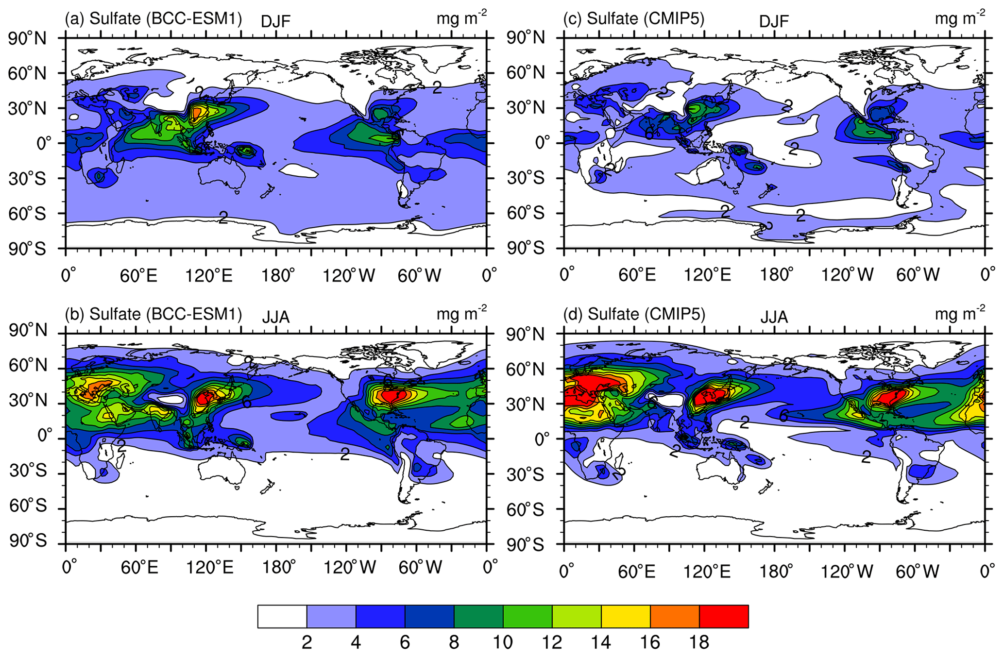
Figure 8December–January–February (DJF; a, c) and June–July–August (JJA; b, d) mean sulfate () aerosol column mass concentrations averaged for the period of 1971–2000. Panels (a, b) show the historical simulations of BCC-ESM1 and (c, d) the CMIP5-recommended data. Units: milligram per square meter.
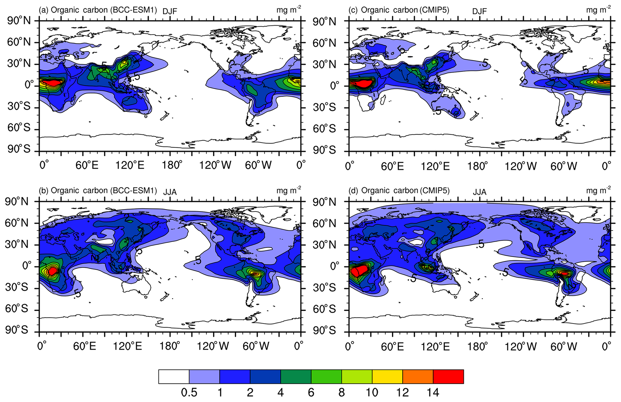
Figure 9The same as in Fig. 8, but for organic carbon (OC) aerosol column mass concentrations. Units: milligram per square meter.

Figure 10The same as in Fig. 8, but for black carbon (BC) aerosol. Units: milligram per square meter.
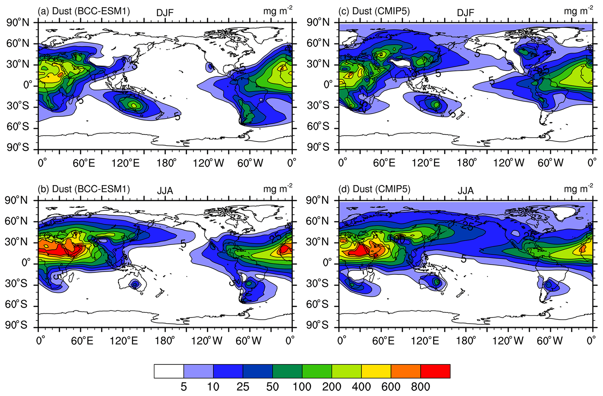
Figure 11The same as in Fig. 8, but for dust aerosol. Units: milligram per square meter.

Figure 12The same as in Fig. 8, but for sea salt (SSLT) aerosol. Units: milligram per square meter.
Unlike sulfate whose maximum concentrations are mainly distributed between 60∘ N and the Equator, peaking concentrations of BC and OC as shown in Figs. 9 and 10 are located near the tropics in the biomass burning regions (e.g., the Maritime Continent, Central Africa, South America), and their seasonal variations from DJF to JJA are evidently weaker than those of sulfate except in South America. In boreal summer, there are centers of high values in the industrial regions in the Northern Hemisphere midlatitudes (i.e., East Asia, South Asia, Europe, and North America). These main features of spatial and seasonal variations in CMIP5 data are well captured by BCC-ESM1, and the BCC-ESM1 vs. CMIP5 spatial correlation coefficients (Fig. 13) are 0.90 (OC in DJF), 0.91 (BC in DJF), 0.91 (OC in JJA), and 0.92 (BC in JJA). There are fewer deviations in spatial pattern for OC in DJF and JJA but larger deviation for BC from CMIP5 data (Fig. 13).
As shown in Fig. 11, dust concentrations in the atmosphere show the largest values over strong source regions such as northern Africa, southwest and Central Asia, and Australia and over their outflow regions such as the Atlantic and the western Pacific. In DJF, the CMIP5 data show centers of high concentrations over East Asia and central North America, but both centers are missing in BCC-ESM1. However, these two high-value centers in the CMIP5 data may not be true, since frozen soils in these areas in winter lead to unfavorable conditions for soil erosion by winds. The spatial correlation coefficients between CMIP5 and BCC-ESM1 remain high: 0.95 in JJA and 0.88 in DJF (Fig. 13). Small deviations in spatial pattern for dust simulations in BCC-ESM1 show a lower magnitude of dust maximums against CMIP5 data (Fig. 13).
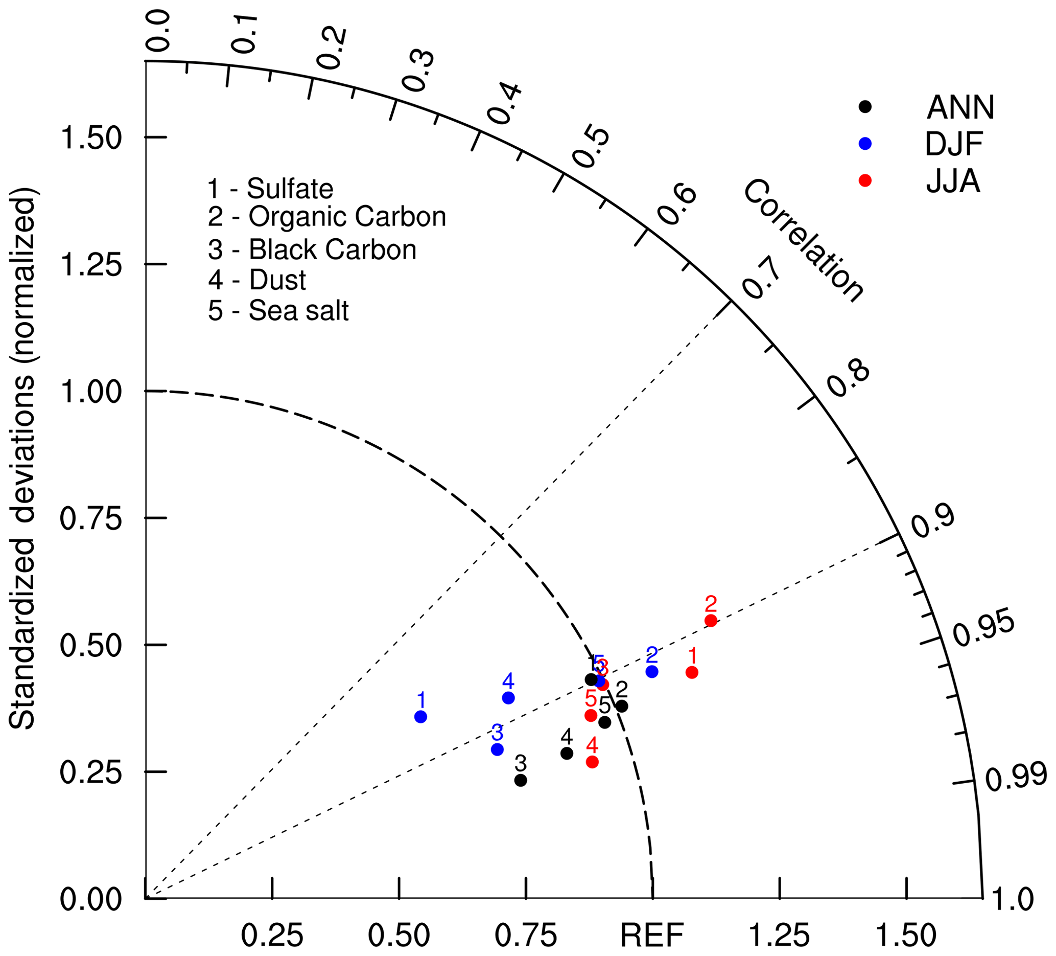
Figure 13Taylor diagram for the global aerosol climatology (1971–2000) of sulfate, organic carbon, black carbon, dust, and sea salt averaged for December–January–February (DJF) and June–July–August (JJA) and annually. The radial coordinate shows the standard deviation in the spatial pattern, normalized by the observed standard deviation. The azimuthal variable shows the correlation of the modeled spatial pattern with the observed spatial pattern. Analysis is for the whole globe. The reference dataset is the CMIP5 prescribed dataset.
As shown in Fig. 12, high sea salt concentrations are generally found over the storm track regions over the oceans, e.g., the midlatitudes in the northern oceans in DJF and the Southern Ocean in JJA, where wind speeds and thus sea salt emissions are higher. In addition, there is a belt of high sea salt concentrations in the subtropics of both hemispheres where precipitation scavenging is weak. Their spatial distributions in BCC-ESM1 are consistent with the CMIP5 data with correlation coefficients of 0.92 in JJA and 0.90 in DJF (Fig. 13). The spatial deviations in sea salt are much closer to CMIP5 data than those of sulfate, OC, BC, and dust distributions (Fig. 13).
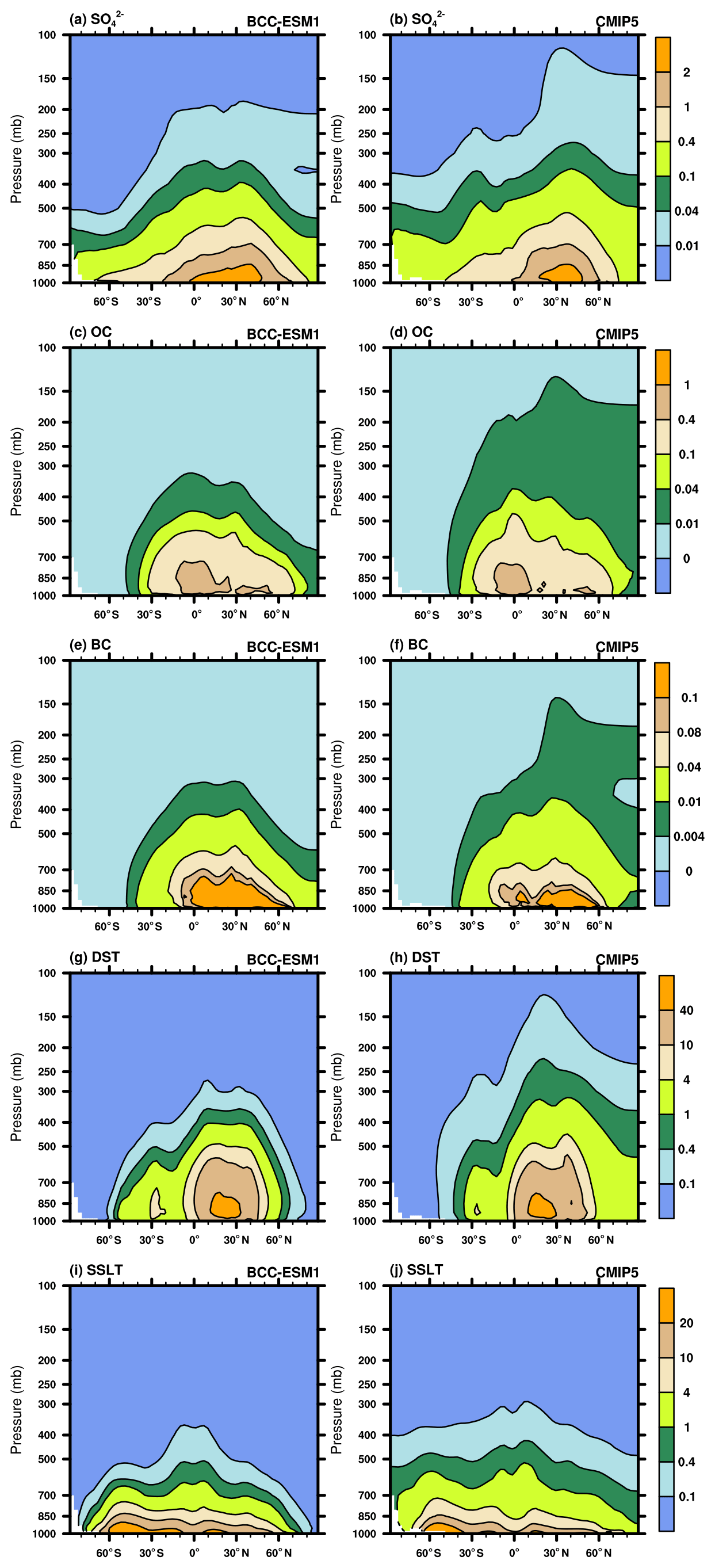
Figure 14Latitude–pressure distributions of zonally averaged annual mean sulfate, organic carbon, black carbon, dust, and sea salt aerosol concentrations for the period of 1971–2000. Left panels show the CMIP6 historical simulation of BCC-ESM1 and right panels the CMIP5 recommendation data. Units: micrograms per cubic meter.
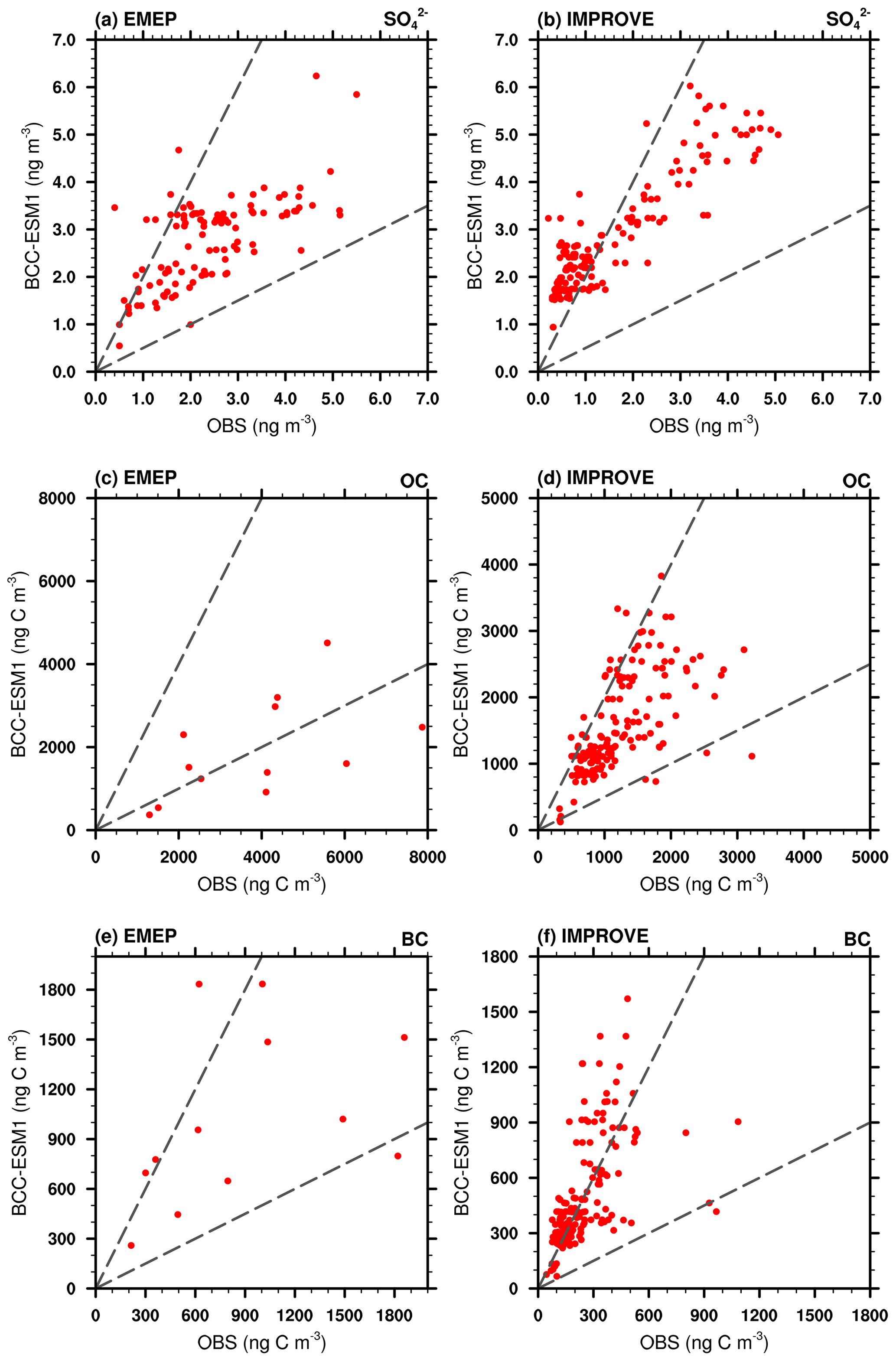
Figure 15Scatterplots showing observed versus simulated multi-year averaged annual mean sulfate (), organic carbon (OC), and black carbon (BC) mixing ratios at the IMPROVE and EMEP network sites. Observations are averages over the available years 1990–2005 for IMPROVE sites and 1995–2005 for EMEP sites. Simulated values are those at the lowest layer of BCC-ESM1.
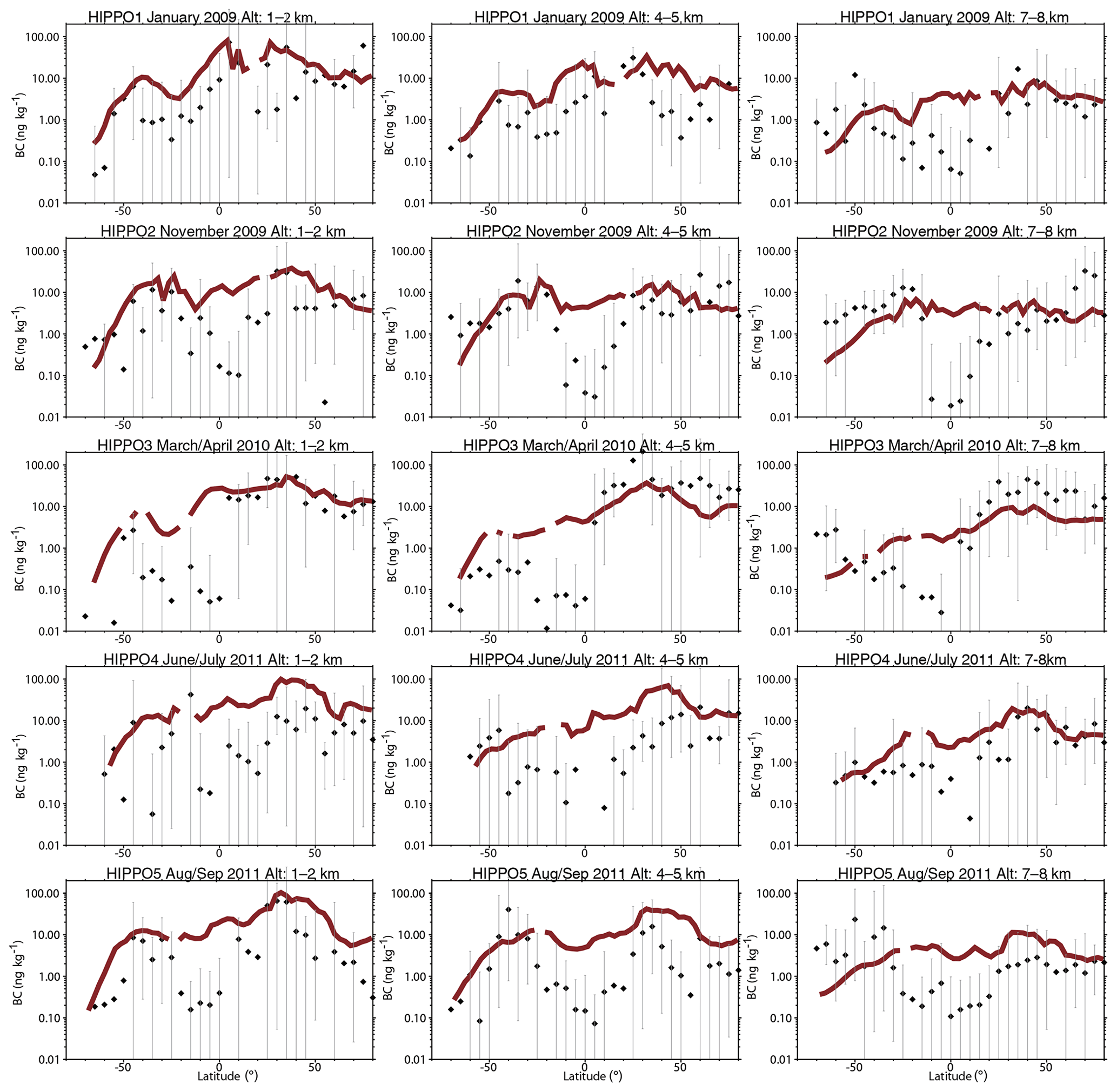
Figure 16Comparison of modeled black carbon (BC) aerosol (red lines) with observations from HIPPO aircraft campaigns over the Pacific Ocean (black symbols; bars represent the full data range). Observations from different HIPPO campaigns were averaged over 5∘ latitude bins and three different altitude bands (left column: 1–2 km; middle column: 4–5 km; and right column: 7–8 km) along the flight track over the Pacific Ocean. Model results were sampled along the flight track and then averaged over the abovementioned regions for comparison.
Figure 14 shows vertical distributions of zonally averaged annual mean concentrations of sulfate, organic carbon, black carbon, dust, and sea salt aerosols in the period of 1991–2000. Both BCC-ESM1 and CMIP5 results show that strong sulfur, OC, and BC emissions in the industrial regions of the Northern Hemisphere midlatitudes can rise upward and be transported towards the North Pole in the mid-troposphere to upper troposphere. Most OC, BC, and dust aerosols are confined to below 500 hPa, while sulfate can be transported to higher altitudes. Sea salt aerosols are mostly confined to below 700 hPa, as the particles are large in size and favorable for wet removal and gravitational settling towards the surface. It can be seen that BCC-ESM1 tends to simulate less upward transport of aerosols than the CMIP5 data, likely reflecting the omission of deep convection transport of tracers in BCC-ESM1.
The CMIP5 data used here are mainly from model simulations. We will further evaluate the BCC-ESM1 model results with ground observations. Annual mean , BC, and OC aerosol observations from the Interagency Monitoring of Protected Visual Environments (IMPROVE) sites over 1990–2005 in the United States (http://vista.cira.colostate.edu/IMPROVE/, last access: 5 October 2019) and from the European Monitoring and Evaluation Programme (EMEP) (http://www.emep.int, last access: 5 October 2019) sites over 1995–2005 are used. As shown in Fig. 15a and b, the BCC-ESM simulated sulfate concentrations are in general comparable to the EMEP observations in Europe but are systematically about 1 µg m−3 higher than the US IMPROVE observations. As for BC, there are large model biases at both European and US sites (Fig. 15c and d); in particular, BCC-ESM overestimates BC concentrations at the IMPROVE sites. The observed OC concentrations are slightly overestimated for IMPROVE sites but systematically underestimated for EMEP sites. Some statistical features for simulated concentrations versus EMEP and IMPROVE observations are listed in Table 7. These comparisons are overall fairly reasonable considering the uncertainties in emissions and the coarse model resolution.
Table 7Observed versus simulated concentrations of sulfate (), organic carbon (OC), and black carbon (BC) for the regional mean and spatial standard deviation and minimum and maximum values at HIPPO aircraft observations (BC only), and IMPROVE and EMEP network sites and the spatial correlation between observed and simulated multi-year averaged annual means. Simulated values are selected for the same locations and the same valid observation time. The data used are the same as those in Fig. 12.
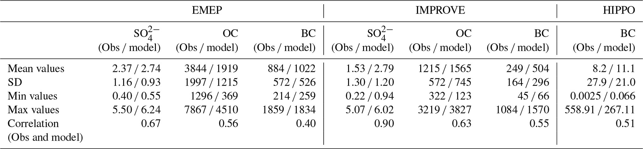
We then evaluate the simulated BC concentrations from BCC-ESM1 with the HIAPER (High-Performance Instrumented Airborne Platform for Environmental Research) Pole-to-Pole Observations (HIPPO) (Wofsy et al., 2011). The HIPPO campaign provided observations of black carbon concentration profiles over the Pacific Ocean and North America between 2009 and 2011. Following Tilmes et al. (2016), model results here are sampled along the HIPPO flight tracks and then averaged to different latitude and altitude bands for comparison. As shown in Fig. 16, BCC-ESM1 and HIPPO aircraft observations shows reasonable agreement in terms of the spatial distributions and seasonal variations in BC levels. BCC-ESM1 generally reproduces the observed hemispheric gradients of BC, i.e., the larger burden in the NH compared to the SH, consistent with Figs. 10 and 14. The mean value of modeled results along the flight track is 11.1 ng kg−1, comparable to the 8.2 ng kg−1 of the HIPPO observations. The model shows large overestimations of BC observations over the tropics, which is also found in the CAM4-chem global chemical model (Tilmes et al., 2016).
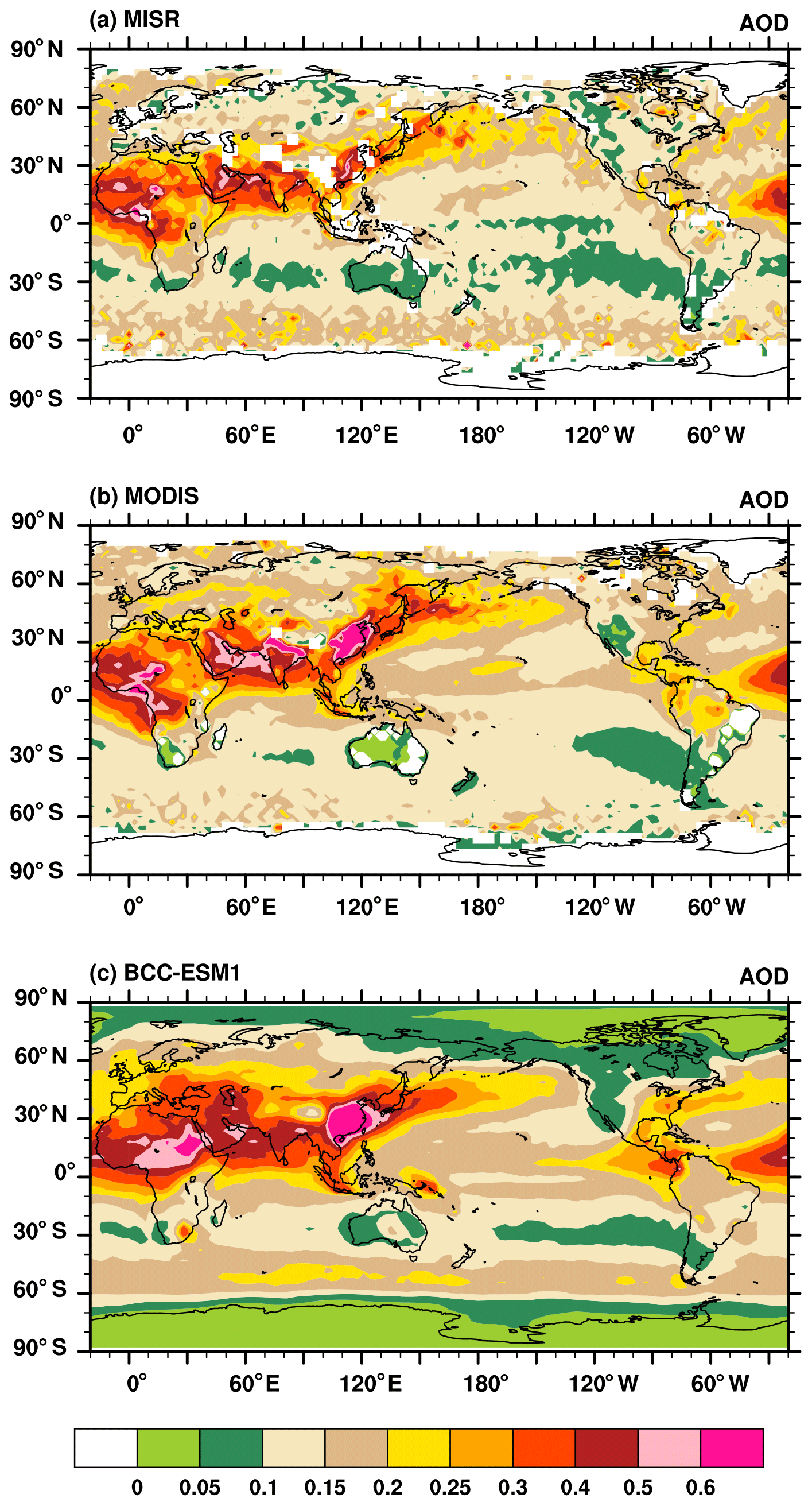
Figure 17Global distribution of annual mean AOD simulated in BCC-ESM1 compared with the MISR and MODIS data for the year 2008.

Figure 18Observed versus simulated annual means of AOD at AERONET sites. Each data point represents the mean averaged for available monthly values of AOD. The dot sizes denote the magnitudes of AOD at sites. The spatial correlation is 0.56.
4.4 Aerosol optical properties
Aerosol optical depth (AOD) is an indicator of the reduction in incoming solar radiation (at a particular wavelength) due to scattering and absorption of sunlight by aerosols. In this study, we calculate the AOD at 550 nm for all aerosols including sulfate, BC, organic carbon, sea salt, and dust as the product of aerosol dry mass concentrations, aerosol water content, and their specific extinction coefficients. The total AOD is calculated by summing the AOD in each model layer for each aerosol species using the assumption that they are externally mixed. The AOD observations retrieved from the Moderate Resolution Imaging Spectroradiometer (MODIS) and the Multi-angle Imaging SpectroRadiometer (MISR) over the period of 1997–2003 and from the AErosol RObotic NETwork (AERONET) over the period of 1998–2005 (http://aeronet.gsfc.nasa.gov, last access: 2 August 2019) are used to evaluate the averaged AOD at 550 nm in BCC-ESM. Figure 17 shows averages of MISR and MODIS AOD with corresponding averages from BCC-ESM. The BCC-ESM1 simulated AOD generally captures the spatial distribution of MISR and MODIS retrievals. The model overestimates AOD over east China. It also systematically underestimates the MODIS observations in the Southern Hemisphere but is closer to MISR observations. Figure 18 shows multi-year annual means of BCC-ESM1-simulated AOD values versus observations from AERONET over the period of 1998–2005. The basic pattern of modeled global AOD is similar to that of observations and their spatial correlation reaches 0.56. Large values of AOD are mainly distributed in land continents such as North African, South Asia, East Asia, Europe, and the eastern part of North America. Figure 19a–d present scatterplots of observed versus simulated multi-year monthly mean AOD at those sites of AERONET in Europe, North America, East Asia, and South Asia over the period of 1998–2005. Model-simulated monthly AOD generally agrees with observations within a factor of 2 for most sites. BCC-ESM slightly overestimates the AOD at European and North American sites. In those regions, BCC-ESM also slightly overestimates MODIS and MISR AOD observations (Fig. 17).
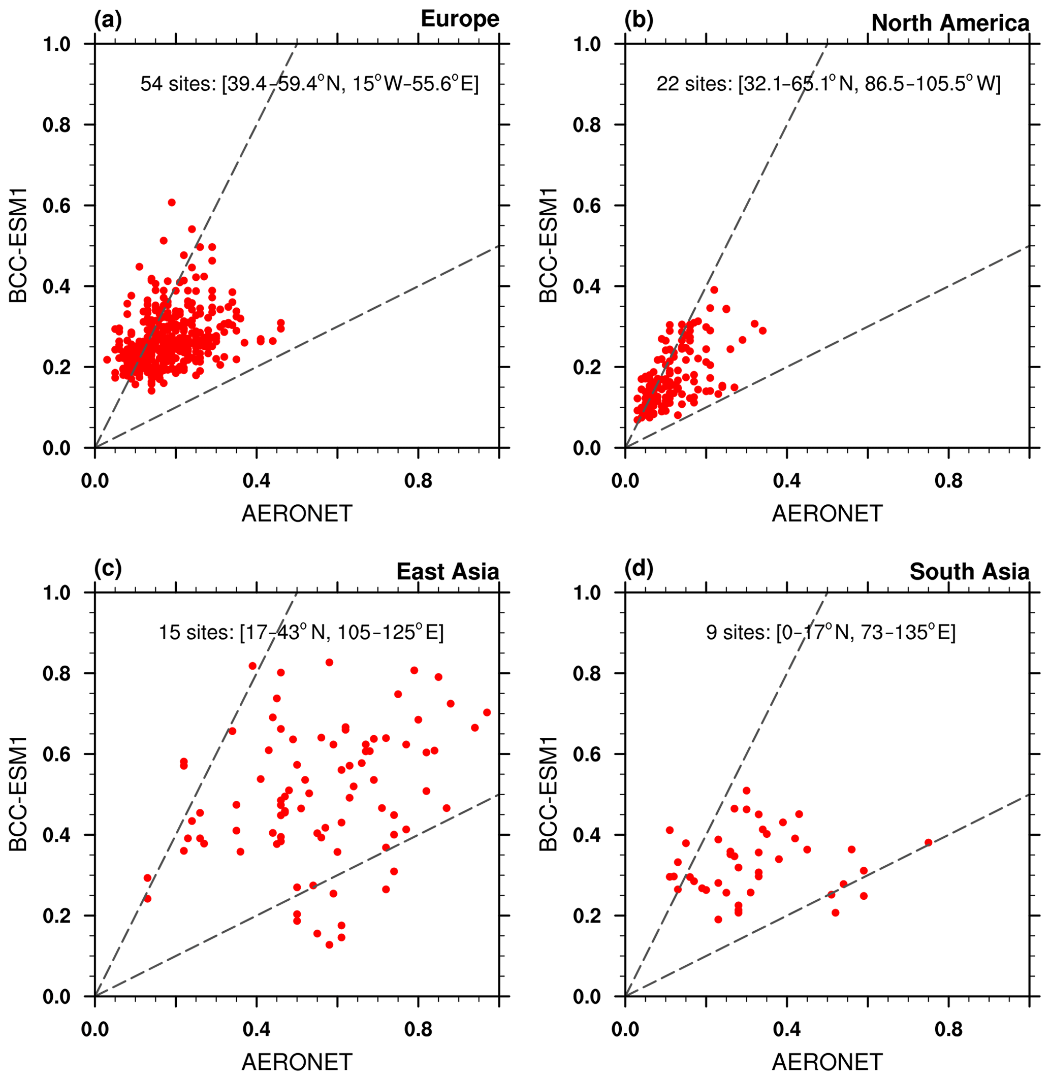
Figure 19Scatterplots of observed versus simulated monthly mean AOD at AERONET sites in Europe, North America, East Asia, and South Asia over the period of 1998–2005.
This paper presents a primary evaluation of aerosols simulated in version 1 of the BCC-ESM1 with the implementation of the interactive atmospheric chemistry and aerosol based on the newly developed BCC-CSM2. Global aerosols (including sulfate, organic carbon, black carbon, dust, and sea salt) and major greenhouse gases (e.g., O3, CH4, N2O) in the atmosphere can be interactively simulated when anthropogenic emissions are provided to the model. Concentrations of all aerosols in BCC-ESM1 are determined by the processes of advective transport, emission, gas-phase chemical reactions, dry deposition, gravitational settling, and wet scavenging by clouds and precipitation. The nucleation and coagulation of aerosols are ignored in the present version of BCC-ESM1. Effects of aerosols on radiation, cloud, and precipitation are fully included.
We evaluate the performance of BCC-ESM1 in simulating aerosols and their optical properties in the 20th century following CMIP6 historical simulation according to the requirement of the AerChemMIP. It is forced with anthropogenic emissions evolving from 1850 to 2014, but some WMGHGs such as CH4, N2O, CO2, CFC11, and CFC12 are prescribed using CMIP6 prescribed concentrations (to replace prognostic values of CH4 and N2O from the chemistry scheme). Both direct and indirect effects of aerosols are considered in BCC-ESM1. Initial conditions of the CMIP6 historical simulation are obtained from a 600-year piControl simulation in the absence of anthropogenic emissions, which captures the preindustrial concentrations of , organic carbon (OC), black carbon (BC), dust, and sea salt aerosols well and is consistent with the CMIP5 recommended concentrations for the year 1850. With the CMIP6 anthropogenic emissions of SO2, OC, and BC from 1850 to 2014 and their natural emissions implemented in BCC-ESM1, the model-simulated , BC, and OC aerosols in the atmosphere are highly correlated with the CMIP5-recommended data. The long-term trends in CMIP5 aerosols from 1850 to 2000 are also well simulated by BCC-ESM1. Global budgets of aerosols were evaluated through comparisons of BCC-ESM1 results for 1990–2000 with reports in various contributions to the literature for sulfate, BC, OC, sea salt, and dust. Their annual total emissions, atmospheric mass loading, and mean lifetimes are all within the range of values reported in the relevant literature. Evaluations of the spatial and vertical distributions of BCC-ESM1 simulated present-day , OC, BC, dust, and sea salt aerosol concentrations against the CMIP5 datasets and in situ measurements of surface networks (IMPROVE in the US and EMEP in Europe), and HIPPO aircraft observations indicate good agreement among them. The BCC-ESM1 simulates weaker upward transport of aerosols from the surface to the middle and upper troposphere (with reference to CMIP5-recommended data), likely reflecting a lack of deep convection transport of chemical species in the present version of BCC-ESM1. The AOD at 550 nm for all aerosols including sulfate, BC, OC, sea salt, and dust aerosols was further compared with the satellite AOD observations retrieved from MODIS and MISR and surface AOD observations from AERONET. The BCC-ESM1 model results are overall in good agreement with these observations within a factor of 2. All these comparisons demonstrate the success of the implementation of interactive aerosol and atmospheric chemistry in BCC-ESM1.
This work has only evaluated the ability of BCC-ESM1 to simulate aerosols. The variations in aerosols especially for sulfate are related to other gaseous tracers such as OH and NO3 (Table 2), which are determined by the MOZART2 gaseous chemical scheme as implemented in BCC-ESM1, and require further evaluation. As the length of the text is limited, the other optical features of aerosols such as extinction coefficients, single-scattering albedo and asymmetry parameters, and even their feedbacks on radiation and global temperature change will be explored in a second part. O3 is evaluated in this work. Other GHGs such as CH4 and N2O concentrations can be simulated when forced with emissions, and their simulations also needs to be evaluated in the future.
The source codes of BCC-ESM1, model input files, and scripts to reproduce the simulations that are presented in the article have been archived and made publicly available for downloading from https://doi.org/10.5281/zenodo.3609337 (Wu et al., 2020). Model output data of BCC CMIP6 AerChemMIP simulations described in this paper are available on the Earth System Grid Federation (ESGF) (https://cera-www.dkrz.de/WDCC/ui/cerasearch/cmip6?input=CMIP6.AerChemMIP.BCC.BCC-ESM1, last access: 8 January 2020, https://doi.org/10.22033/ESGF/CMIP6.1733; Zhang et al., 2019). Details about ESGF are presented on the CMIP panel website at http://www.wcrp-climate.org/index.php/wgcm-cmip/about-cmip (last access: 8 January 2020).
All the figures are created by the NCAR Command Language (Version 6.6.2, 2019).
TW led the BCC-ESM1 development. All other co-authors contributed to it. FZ and JZ designed the experiments and carried them out. TW, LL, LZ, XL, AH, and JW wrote the final document with contributions from all other authors.
The authors declare that they have no conflict of interest.
This research has been supported by the The National Key Research and Development Program of China (grant no. 2016YFA0602100).
This paper was edited by Fiona O'Connor and reviewed by Jean-Francois Lamarque and one anonymous referee.
Albani, S., Mahowald, N. M., Perry, A. T., Scanza, R. A., Zender, C. S., Heavens, N. G., Maggi, V., Kok, J. F., and Otto-Bliesner, B. L.: Improved dust representation in the Community Atmosphere Model, J. Adv. Model. Earth Syst., 6, 541–570, https://doi.org/10.1002/2013MS000279, 2014.
Albrecht, B.: Aerosols, cloud microphysics, and fractional cloudiness, Science, 245, 1227–1230, 1989.
Arora, V., Boer, G., Friedlingstein, P., Eby, M., Jones, C., Christian, J., Bonan, G., Bopp, L., Brovkin, V., Cadule, P., Hajima, T., Ilyina, T., Lindsay, K., Tjiputra, J., and Wu, T.: Carbon-concentration and carbon-climate feedbacks in CMIP5 Earth system models, J. Climate, 26, 5289–5314, 2013.
Austin, J., Butchart, N., and Shine, K. P.: Possibility of an Arctic ozone hole in a doubled-CO2 climate, Nature, 360, 221–225, 1992
Barth, M. C., Rasch, P. J., Kiehl, J. T., Benkowitz, C. M., and Schwartz, S. E.: Sulfur chemistry in the National Center for Atmospheric Research Community Climate Model: Description, evaluation, features, and sensitivity to aqueous chemistry, J. Geophys. Res., 105, 1387–1415, 2000.
Bey I., Jacob, D. J., Yantosca, R. M., Logan, J. A., Field, B., Fiore, A. M., Li, Q., Liu, H., Mickley, L. J., and Schultz, M.: Global modeling of tropospheric chemistry with assimilated meteorology: Model description and evaluation, J. Geophys. Res., 106, 23073–23096, 2001
Boucher, O. and Lohmann, U.: The sulphate-CCN-cloud albedo effect – a sensitivity study with two general circulation models, Tellus B, 47, 281–300, 1995.
Brasseur, G. P., Tie, X. X., Rasch, P. J., and Lefèvre, F.: A three-dimensional simulation of the Antarctic ozone hole: Impact of anthropogenic chlorine on the lower stratosphere and upper troposphere, J. Geophys. Res., 102, 8909–8930, 1997.
Brasseur, G. P., Hauglustaine, D. A., Walters, S., Rasch, P. J., Müller, J.-F., Granier, C., and Tie, X. X.: MOZART, a global chemical transport model for ozone and related chemical tracers: 1. Model description, J. Geophys. Res., 103, 28265– 28289, 1998.
Cariolle, D., Lasserre-Bigorry, A., and Royer, J.-F.: A general circulation model simulation of the springtime Antarctic ozone decrease and its impact on midlatitudes, J. Geophys. Res., 95, 1883–1898, 1990.
Chen, C. and Cotton, W. R.: The physics of the marine stratocumulus-capped mixed layer, J. Atmos. Sci., 44, 2951–2977, 1987.
Chin, M., Ginoux, P., Kinne, S., Torres, O., Holben, B. N., Duncan, B. N., Martin, R. V., Logan, J. A., Higurashi, A., and Naka-jima, T.: Tropospheric aerosol optical thickness from the GOCART model and comparisons with satellite and Sun photometer measurements, J. Atmos. Sci., 59, 461–483, 2002.
Chuang, C. C., Penner, J. E., Taylor, K. E., Grossman, A. S., and Walton, J. J.: An assessment of the radiative effects of anthropogenic sulfate, J. Geophys. Res., 102, 3761–3778, 1997.
Collins, W. D., Rasch, P. J., Boville, B. A., Hack, J. J., McCaa, J. R., Williamson, D. L,. Kiehl, J. T., Briegleb, B. P., Bitz, C., Lin, S.-J., Zhang, M., and Dai, Y.: Description of the NCAR Community Atmosphere Model (CAM3), Nat. Cent. for Atmos. Res., Boulder, CO, 2004.
Collins, W. J., Lamarque, J.-F., Schulz, M., Boucher, O., Eyring, V., Hegglin, M. I., Maycock, A., Myhre, G., Prather, M., Shindell, D., and Smith, S. J.: AerChemMIP: quantifying the effects of chemistry and aerosols in CMIP6, Geosci. Model Dev., 10, 585–607, https://doi.org/10.5194/gmd-10-585-2017, 2017.
Cooke, W. F. and Wilson, J. J. N.: A global black carbon aerosol model, J. Geophys. Res.-Atmos., 101, 19395–19409, 1996.
Cunnold, D., Alyea, F., Phillips, N., and Prinn, R.: A three-dimensional dynamical-chemical model of atmospheric ozone, J. Atmos. Sci., 32, 170–194, 1975.
Dentener, F., Kinne, S., Bond, T., Boucher, O., Cofala, J., Generoso, S., Ginoux, P., Gong, S., Hoelzemann, J. J., Ito, A., Marelli, L., Penner, J. E., Putaud, J.-P., Textor, C., Schulz, M., van der Werf, G. R., and Wilson, J.: Emissions of primary aerosol and precursor gases in the years 2000 and 1750 prescribed data-sets for AeroCom, Atmos. Chem. Phys., 6, 4321–4344, https://doi.org/10.5194/acp-6-4321-2006, 2006.
Eyring, V., Bony, S., Meehl, G. A., Senior, C. A., Stevens, B., Stouffer, R. J., and Taylor, K. E.: Overview of the Coupled Model Intercomparison Project Phase 6 (CMIP6) experimental design and organization, Geosci. Model Dev., 9, 1937–1958, https://doi.org/10.5194/gmd-9-1937-2016, 2016.
Feichter, J., Kjellstrom, E., Rodhe, H., Dentener, F., Lelieveldi, J., and Roelofs, G.-J.: Simulation of the tropospheric sulfur cycle in a global climate model, Atmos. Environ., 30, 1693–1707, 1996.
Feng, L., Smith, S. J., Braun, C., Crippa, M., Gidden, M. J., Hoesly, R., Klimont, Z., van Marle, M., van den Berg, M., and van der Werf, G. R.: The generation of gridded emissions data for CMIP6, Geosci. Model Dev., 13, 461–482, https://doi.org/10.5194/gmd-13-461-2020, 2020.
Ghan, S. J. and Easter, R. C.: Impact of cloud-borne aerosol representation on aerosol direct and indirect effects, Atmos. Chem. Phys., 6, 4163–4174, https://doi.org/10.5194/acp-6-4163-2006, 2006.
Ginoux, P., Chin, M., Tegen, I., Prospero, J. M., Holben, B., Dubovik, O., and Lin, S.-J.: Sources and distributions of dust aerosols simulated with the GOCART model, J. Geophys. Res., 106, 20255–20274, 2001.
Giorgi, F. and Chameides, W. L.: The rainout parameterization in a photochemical model, J. Geophys. Res., 90, 7872–7880, 1985.
Guenther, A., Baugh, B. Brasseur, G., Greenberg, J., Harley, P., Klinger, L,. Serca, D., and Vierling, L.: Isoprene emission estimates and uncertainties for the Central African EXPRESSO study domain, J. Geophys. Res., 104, 30, 625–630, 639, 1999.
Guenther, A. B., Jiang, X., Heald, C. L., Sakulyanontvittaya, T., Duhl, T., Emmons, L. K., and Wang, X.: The Model of Emissions of Gases and Aerosols from Nature version 2.1 (MEGAN2.1): an extended and updated framework for modeling biogenic emissions, Geosci. Model Dev., 5, 1471–1492, https://doi.org/10.5194/gmd-5-1471-2012, 2012.
Hess, M., Koepke, P., and Schult, I.: Optical properties of aerosols and clouds: the software package OPAC, B. Am. Meteorol. Soc., 79, 831–844, 1998.
Hoesly, R. M., Smith, S. J., Feng, L., Klimont, Z., Janssens-Maenhout, G., Pitkanen, T., Seibert, J. J., Vu, L., Andres, R. J., Bolt, R. M., Bond, T. C., Dawidowski, L., Kholod, N., Kurokawa, J.-I., Li, M., Liu, L., Lu, Z., Moura, M. C. P., O'Rourke, P. R., and Zhang, Q.: Historical (1750–2014) anthropogenic emissions of reactive gases and aerosols from the Community Emissions Data System (CEDS), Geosci. Model Dev., 11, 369–408, https://doi.org/10.5194/gmd-11-369-2018, 2018.
Horowitz, L. W.: Past, present, and future concentrations of tropospheric ozone and aerosols: Methodology, ozone evaluation, and sensitivity to aerosol wet removal, J. Geophys. Res., 111, D22211, https://doi.org/10.1029/2005JD006937, 2006.
Horowitz, L. W., Walters, S., Mauzerall, D. L., Emmons, L. K., Rasch, P. J., Granier, C., Tie, X., Lamarque, J.-F., Schultz, M. G., Tyndall, G. S., Orlando, J. J., and Brasseur, G. P.: A global simulation of tropospheric ozone and related tracers: Description and evaluation of MOZART, version 2, J. Geophys. Res., 108, 4784, https://doi.org/10.1029/2002JD002853, 2003.
Hoffman, F. M., Randerson, J. T., Arora, V. K., Bao, Q., Cadule, P., Ji, D., Jones, C. D., Kawamiya, M., Khatiwala, S., Lindsay, K., Obata, A., Shevliakova, E., Six, K. D., Tjiputra, J. F., Volodin, E. M., and Wu, T.: Causes and implications of persistent atmospheric carbon dioxide biases in Earth System Models, J. Geophys. Res.-Biogeo., 119, 141–162, https://doi.org/10.1002/2013JG002381, 2014.
Holtslag, A. A. M. and Boville, B. A.: Local versus nonlocal boundary-layer diffusion in a global climate model, J. Climate, 6, 1825–1842, 1993.
Hurtt, G. C., Chini, L. P., Frolking, S., Betts, R. A., Feddema, J., Fischer, G., Fisk, J. P., Hibbard, K., Houghton, R. A., Janetos, A., Jones, C. D., Kindermann, G., Kinoshita, T., Goldewijk, K. K., Riahi, K., Shevliakova,E., Smith, S., Stehfest, E.,Thomson, A., Thornton, P., van Vuuren, and D. P., Wang, Y. P.: Harmonization of land-use scenarios for the period 1500–2100: 600 years of global gridded annual land-use transitions, wood harvest, and resulting secondary lands, Clim. Change, 109, 117–161, 2011.
Hurtt, G., Chini, L., Sahajpal, R., Frolking, S., Bodirsky, B. L., Calvin, K., Doelman, J., Fisk, J., Fujimori, S., Goldewijk, K. K., Hasegawa, T., Havlik, P., Heinimann, A., Humpenöder, F., Jungclaus, J., Kaplan, J., Krisztin, T., Lawrence, D., Lawrence, P., Mertz, O., Pongratz, J., Popp, A., Riahi, K., Shevliakova, E., Stehfest, E., Thornton, P., van Vuuren, D., and Zhang, X.: input4MIPs.UofMD.landState.CMIP.UofMD-landState-2-1-h, version 20170126, Earth Syst. Grid Fed., https://doi.org/10.22033/ESGF/input4MIPs.1127, 2017.
Jacobson, M. Z.: Investigating cloud absorption effects: global absorption properties of black carbon, tar balls, and soil dust in clouds and aerosols, J. Geophys. Res. 117, D06205, https://doi.org/10.1029/2011JD017218, 2012.
Jones, C. D., Arora, V., Friedlingstein, P., Bopp, L., Brovkin, V., Dunne, J., Graven, H., Hoffman, F., Ilyina, T., John, J. G., Jung, M., Kawamiya, M., Koven, C., Pongratz, J., Raddatz, T., Randerson, J. T., and Zaehle, S.: C4MIP – The Coupled Climate–Carbon Cycle Model Intercomparison Project: experimental protocol for CMIP6, Geosci. Model Dev., 9, 2853–2880, https://doi.org/10.5194/gmd-9-2853-2016, 2016.
Lamarque, J.-F., Bond, T. C., Eyring, V., Granier, C., Heil, A., Klimont, Z., Lee, D., Liousse, C., Mieville, A., Owen, B., Schultz, M. G., Shindell, D., Smith, S. J., Stehfest, E., Van Aardenne, J., Cooper, O. R., Kainuma, M., Mahowald, N., McConnell, J. R., Naik, V., Riahi, K., and van Vuuren, D. P.: Historical (1850–2000) gridded anthropogenic and biomass burning emissions of reactive gases and aerosols: methodology and application, Atmos. Chem. Phys., 10, 7017–7039, https://doi.org/10.5194/acp-10-7017-2010, 2010.
Lamarque, J.-F., Emmons, L. K., Hess, P. G., Kinnison, D. E., Tilmes, S., Vitt, F., Heald, C. L., Holland, E. A., Lauritzen, P. H., Neu, J., Orlando, J. J., Rasch, P. J., and Tyndall, G. K.: CAM-chem: description and evaluation of interactive atmospheric chemistry in the Community Earth System Model, Geosci. Model Dev., 5, 369–411, https://doi.org/10.5194/gmd-5-369-2012, 2012.
Lamarque, J.-F., Shindell, D. T., Josse, B., Young, P. J., Cionni, I., Eyring, V., Bergmann, D., Cameron-Smith, P., Collins, W. J., Doherty, R., Dalsoren, S., Faluvegi, G., Folberth, G., Ghan, S. J., Horowitz, L. W., Lee, Y. H., MacKenzie, I. A., Nagashima, T., Naik, V., Plummer, D., Righi, M., Rumbold, S. T., Schulz, M., Skeie, R. B., Stevenson, D. S., Strode, S., Sudo, K., Szopa, S., Voulgarakis, A., and Zeng, G.: The Atmospheric Chemistry and Climate Model Intercomparison Project (ACCMIP): overview and description of models, simulations and climate diagnostics, Geosci. Model Dev., 6, 179–206, https://doi.org/10.5194/gmd-6-179-2013, 2013.
Li, W., Zhang, Y., Shi, X., Zhou, W., Huang, A., Mu, M., Qiu, B., and Ji, J.: Development of the Land Surface Model BCC_AVIM2.0 and Its Preliminary Performance in LS3MIP/CMIP6, J. Meteor. Res., 33, 851–869, https://doi.org/10.1007/s13351-019-9016-y, 2019.
Liu, J., Mauzerall, D. L., Horowitz, L. W., Ginoux, P., and Fiore, A. M.: Evaluation intercontinental transport of fine aerosols: (1) methodology, global aerosol distribution and optical depth, Atmos. Environ., 43, 4327–4338, 2009.
Liu, X. H., Penner, J. E., and Herzog, M.: Global modeling of aerosol dynamics: Model description, evaluation, and interactions between sulfate and nonsulfate aerosols, J. Geophys. Res.-Atmos., 110, D18206, https://doi.org/10.1029/2004jd005674, 2005.
Liu, X., Easter, R. C., Ghan, S. J., Zaveri, R., Rasch, P., Shi, X., Lamarque, J.-F., Gettelman, A., Morrison, H., Vitt, F., Conley, A., Park, S., Neale, R., Hannay, C., Ekman, A. M. L., Hess, P., Mahowald, N., Collins, W., Iacono, M. J., Bretherton, C. S., Flanner, M. G., and Mitchell, D.: Toward a minimal representation of aerosols in climate models: description and evaluation in the Community Atmosphere Model CAM5, Geosci. Model Dev., 5, 709–739, https://doi.org/10.5194/gmd-5-709-2012, 2012.
Liu, X., Ma, P.-L., Wang, H., Tilmes, S., Singh, B., Easter, R. C., Ghan, S. J., and Rasch, P. J.: Description and evaluation of a new four-mode version of the Modal Aerosol Module (MAM4) within version 5.3 of the Community Atmosphere Model, Geosci. Model Dev., 9, 505–522, https://doi.org/10.5194/gmd-9-505-2016, 2016.
Lohmann, U., Feichter, J., Penner, J. E., and Leaitch, W. R.: Indirect effect of sulfate and carbonaceous aerosols: A mechanistic treatment, J. Geophys. Res., 105, 12193–12206, 2000.
Lu, X., Zhang, L., Wu, T., Long, M. S., Wang, J., Jacob, D. J., Zhang, F., Zhang, J., Eastham, S. D., Hu, L., Zhu, L., Liu, X., and Wei, M.: Development of the global atmospheric general circulation-chemistry model BCC-GEOS-Chem v1.0: model description and evaluation, Geosci. Model Dev. Discuss., https://doi.org/10.5194/gmd-2019-240, in review, 2019.
Mahowald, N., Lamarque, J.-F., Tie, X., and Wolff, E.: Sea salt aerosol response to climate change: last glacial maximum, preindustrial and doubled carbon dioxide climates, J. Geophys. Res., 111, D05303, https://doi.org/10.1029/2005JD006459, 2006.
Martin, R. V., Jacob, D. J., Logan, J. A., Bey, I., Yantosca, R. M., Staudt, A. C., Li, Q., Fiore, A. M., Duncan, B. N., Liu, H., Ginoux, P., and Thouret, V.: Interpretation of TOMS observations of tropical tropospheric ozone with a global model and in situ observations, J. Geophys. Res., 107, 4351, https://doi.org/10.1029/2001JD001480, 2002.
Matsui, H. and Mahowald, N.: Development of a global aerosol model using a two-dimensional sectional method: 2. Evaluation and sensitivity simulations, J. Adv. Model. Earth Syst., 9, 1887–1920, https://doi.org/10.1002/2017MS000937, 2017.
Matthes, K., Funke, B., Andersson, M. E., Barnard, L., Beer, J., Charbonneau, P., Clilverd, M. A., Dudok de Wit, T., Haberreiter, M., Hendry, A., Jackman, C. H., Kretzschmar, M., Kruschke, T., Kunze, M., Langematz, U., Marsh, D. R., Maycock, A. C., Misios, S., Rodger, C. J., Scaife, A. A., Seppälä, A., Shangguan, M., Sinnhuber, M., Tourpali, K., Usoskin, I., van de Kamp, M., Verronen, P. T., and Versick, S.: Solar forcing for CMIP6 (v3.2), Geosci. Model Dev., 10, 2247–2302, https://doi.org/10.5194/gmd-10-2247-2017, 2017.
Meinshausen, M., Vogel, E., Nauels, A., Lorbacher, K., Meinshausen, N., Etheridge, D. M., Fraser, P. J., Montzka, S. A., Rayner, P. J., Trudinger, C. M., Krummel, P. B., Beyerle, U., Canadell, J. G., Daniel, J. S., Enting, I. G., Law, R. M., Lunder, C. R., O'Doherty, S., Prinn, R. G., Reimann, S., Rubino, M., Velders, G. J. M., Vollmer, M. K., Wang, R. H. J., and Weiss, R.: Historical greenhouse gas concentrations for climate modelling (CMIP6), Geosci. Model Dev., 10, 2057–2116, https://doi.org/10.5194/gmd-10-2057-2017, 2017.
Mora, C., Wei, C.-L., Rollo, A., Amaro, T., Baco, A. R., Billett, D., Bopp, L., Chen, Q., Collier, M., Danovaro, R., Gooday, A. J., Grupe, B. M., Halloran, P. R., Ingels, J., Jones, D. O. B., Levin, L. A., Nakano, H., Norling, K., Ramirez-Llodra, E., Rex, M., Ruh, H. A., Smith, C. R., Sweetman, A. K., Thurber, A. R., Tjiputra, J. F., Usseglio, P., Watling, L., Wu, T., and Yasuhara, M.: Biotic and human vulnerability to projected ocean biogeochemistry change over the 21st century, PLoS Biol 11, e1001682, https://doi.org/10.1371/journal.pbio.1001682, 2013.
NCAR Command Language (Version 6.6.2), Software, Boulder, Colorado: UCAR/NCAR/CISL/TDD, https://doi.org/10.5065/D6WD3XH5, 2019.
Neale, R. B., Richter, J. H., Conley, A. J., Park, S., Lauritzen, P. H., Gettelman, A., Williamson, D. L., Rasch, P. J., Vavrus, S. J., Taylor, M. A., Collins, W. D., Zhang, M., and Lin, S.-J.: Description of the NCAR Community Atmosphere Model (CAM 4.0), NCAR Tech. Note, TN-485, Natl. Cent. for Atmos. Res., Boulder, CO, 212 pp., 2010.
Neu, J. L. and Prather, M. J.: Toward a more physical representation of precipitation scavenging in global chemistry models: cloud overlap and ice physics and their impact on tropospheric ozone, Atmos. Chem. Phys., 12, 3289–3310, https://doi.org/10.5194/acp-12-3289-2012, 2012.
Olivier, J. G. J., Bouwman, A. F., Van der Maas, C. W. M., Berdowski, J. J. M., Veldt, C., Bloos, J. P. J., Visschedijk, A. J. H., Zandveld, P. Y. J., and Haverslag, J. L.: Description of EDGAR Version 2.0: A set of global emission inventories of greenhouse gases and ozone depleting substances for all anthropogenic and most natural sources on a per country basis and on grid, RIVM Techn. Report no. 771060002, TNO-MEP report no. R96/11, Nat. Inst. Of Public Health and the Environment/Netherlands Organisation for Applied Scientific Research, Bilthoven, 1996.
Peng, Y. and Lohmann, U.: Sensitivity study of the spectral dispersion of the cloud droplet size distribution on the indirect aerosol effect, Geophys. Res. Lett., 30, 1507, https://doi.org/10.1029/2003GL017192, 2003.
Price, C. and Rind, D.: A simple lightning parameterization for calculating global lightning distributions, J. Geophys. Res., 97, 9919–9933, 1992.
Quaas, J., Boucher, O., and Lohmann, U.: Constraining the total aerosol indirect effect in the LMDZ and ECHAM4 GCMs using MODIS satellite data, Atmos. Chem. Phys., 6, 947–955, https://doi.org/10.5194/acp-6-947-2006, 2006.
Sander, S.P., Friedl, R.R., Golden, D. M., Kurylo, M. J., Huie, R. E., Orkin, V. L., Moortgat, G. K., Ravishankara, A. R., Kolb, C. E., Molina, M. J., and Finlayson-Pitts, B. J.: Chemical Kinetics and Photochemical Data for Use in Atmospheric Studies, Evaluation Number 14, JPL Publication 02-25, NASA, Jet Propulsion Laboratory, California Institute of Technology, Pasadena, CA, 2003.
Schlesinger, M. E. and Mintz, Y.: Numerical simulation of ozone production, transport and distribution with a global atmospheric general circulation model, J. Atmos. Sci., 36, 1325–1361, 1979.
Shindell, D. T., Horowitz, L. W., and Schwarzkopf, M. D.: Composition Models in Climate Projections Based on Emissions Scenarios for Long-Lived and Short-Lived Radiatively Active Gases and Aerosols, A Report by the U.S. Climate Change Science Program and the Subcommittee on Global Change Research, edited by: Levy II, H., Shindell, D. T., Gilliland, A.,Schwarzkopf, M. D., Horowitz, L. W., Washington, DC, 2008.
Solomon, S.: Stratospheric ozone depletion: A review of concepts and history, Rev. Geophys., 37, 275–316, 1999.
Taylor, K. E., Stouffer, R. J., and Meehl, G. A.: An overview of CMIP5 and the experiment design, B. Am. Meteorol. Soc., 93, 485–498, 2012.
Tegen, I., Neubauer, D., Ferrachat, S., Siegenthaler-Le Drian, C., Bey, I., Schutgens, N., Stier, P., Watson-Parris, D., Stanelle, T., Schmidt, H., Rast, S., Kokkola, H., Schultz, M., Schroeder, S., Daskalakis, N., Barthel, S., Heinold, B., and Lohmann, U.: The global aerosol–climate model ECHAM6.3–HAM2.3 – Part 1: Aerosol evaluation, Geosci. Model Dev., 12, 1643–1677, https://doi.org/10.5194/gmd-12-1643-2019, 2019.
Textor, C., Schulz, M., Guibert, S., Kinne, S., Balkanski, Y., Bauer, S., Berntsen, T., Berglen, T., Boucher, O., Chin, M., Dentener, F., Diehl, T., Easter, R., Feichter, H., Fillmore, D., Ghan, S., Ginoux, P., Gong, S., Grini, A., Hendricks, J., Horowitz, L., Huang, P., Isaksen, I., Iversen, I., Kloster, S., Koch, D., Kirkevåg, A., Kristjansson, J. E., Krol, M., Lauer, A., Lamarque, J. F., Liu, X., Montanaro, V., Myhre, G., Penner, J., Pitari, G., Reddy, S., Seland, Ø., Stier, P., Takemura, T., and Tie, X.: Analysis and quantification of the diversities of aerosol life cycles within AeroCom, Atmos. Chem. Phys., 6, 1777–1813, https://doi.org/10.5194/acp-6-1777-2006, 2006.
Thomason, L. W., Ernest, N., Millán, L., Rieger, L., Bourassa, A., Vernier, J.-P., Manney, G., Luo, B., Arfeuille, F., and Peter, T.: A global space-based stratospheric aerosol climatology: 1979–2016, Earth Syst. Sci. Data, 10, 469–492, https://doi.org/10.5194/essd-10-469-2018, 2018.
Tie, X., Brasseur, G., Emmons, L., Horowitz, L., and Kinnison, D.: Effects of aerosols on tropospheric oxidants: A global model study, J. Geophys. Res., 106, 2931–2964, 2001.
Tie, X., Madronich, S., Walters, S., Edwards, D., Ginoux, P., Mahowald, N., Zhang, R., Luo, C., and Brasseur, G.: Assessment of the global impact of aerosols on tropospheric oxidants, J. Geophys. Res., 110, D03204, https://doi.org/10.1029/2004JD005359, 2005.
Tilmes, S., Lamarque, J.-F., Emmons, L. K., Kinnison, D. E., Marsh, D., Garcia, R. R., Smith, A. K., Neely, R. R., Conley, A., Vitt, F., Val Martin, M., Tanimoto, H., Simpson, I., Blake, D. R., and Blake, N.: Representation of the Community Earth System Model (CESM1) CAM4-chem within the Chemistry-Climate Model Initiative (CCMI), Geosci. Model Dev., 9, 1853–1890, https://doi.org/10.5194/gmd-9-1853-2016, 2016.
Todd-Brown, K. E. O., Randerson, J. T., Hopkins, F., Arora, V., Hajima, T., Jones, C., Shevliakova, E., Tjiputra, J., Volodin, E., Wu, T., Zhang, Q., and Allison, S. D.: Changes in soil organic carbon storage predicted by Earth system models during the 21st century, Biogeosciences, 11, 2341–2356, https://doi.org/10.5194/bg-11-2341-2014, 2014.
van Marle, M. J. E., Kloster, S., Magi, B. I., Marlon, J. R., Daniau, A.-L., Field, R. D., Arneth, A., Forrest, M., Hantson, S., Kehrwald, N. M., Knorr, W., Lasslop, G., Li, F., Mangeon, S., Yue, C., Kaiser, J. W., and van der Werf, G. R.: Historic global biomass burning emissions for CMIP6 (BB4CMIP) based on merging satellite observations with proxies and fire models (1750–2015), Geosci. Model Dev., 10, 3329–3357, https://doi.org/10.5194/gmd-10-3329-2017, 2017.
Wang, J., Hoffmann, A. A., Park, R., Jacob, D. J., and Martin, S. T.: Global distribution of solid and aqueous sulfate aerosols: effect of the hysteresis of particle phase transitions, J. Geophys. Res., 113, D11206, https://doi.org/10.11029/12007JD009367, 2008a.
Wang, J., Jacob, D. J., and Martin, S. T.: Sensitivity of sulfate direct climate forcing to the hysteresis of particle phase transitions, J. Geophys. Res., 113, D11207, https://doi.org/10.11029/12007JD009368, 2008b.
Wesely, M. L.: Parameterization of surface resistance to gaseous dry deposition in regional-scale numerical models, Atmos. Environ., 23, 1293–1304, 1989.
Wild, M., Folini, D., Schar, C., Loeb, N., Dutton, E. G., and Konig-Langlo, G.: The global energy balance from a surface perspective, Clim. Dynam., 40, 3107–3134, 2013.
Williamson, D. L. and Rasch, P. J.: Two-dimensional semi-Lagrangian transport with shapepreserving interpolation, Mon. Weather Rev., 117, 102–129, 1989.
Wofsy, S. C. and the HIPPO team: HIAPER Pole-to-Pole Observations (HIPPO): fine-grained, global-scale measurements of climatically important atmospheric gases and aerosols, Philos. T. R. Soc. A, 369, 2073–86, https://doi.org/10.1098/rsta.2010.0313, 2011.
Wu, T., Li, W., Ji, J., Xin, X., Li, L., Wang, Z, Zhang, Y., Li, J., Zhang, F., Wei, M., Shi, X., Wu, F., Zhang, L., Chu, M., Jie, W., Liu, Y., Wang, F., Liu, X., Li, Q., Dong, M., Liang, X., Gao, Y., and Zhang, J.: Global carbon budgets simulated by the Beijing climate center climate system model for the last century, J. Geophys. Res.-Atmos., 118, 4326–4347, https://doi.org/10.1002/jgrd.50320, 2013.
Wu, T., Song, L., Li, W., Wang, Z., Zhang, H., Xin, X., Zhang, Y., Zhang, L., Li, J., Wu, F., Liu, Y., Zhang, F., Shi, X., Chu, M., Zhang, J., Fang, Y., Wang, F., Lu, Y., Liu, X., Wei, M., Liu, Q., Zhou, W., Dong, M., Zhao, Q., Ji, J., Li, L., and Zhou, M.: An overview of BCC climate system model development and application for climate change studies, J. Meteor. Res., 28, 34–56, 2014.
Wu, T., Lu, Y., Fang, Y., Xin, X., Li, L., Li, W., Jie, W., Zhang, J., Liu, Y., Zhang, L., Zhang, F., Zhang, Y., Wu, F., Li, J., Chu, M., Wang, Z., Shi, X., Liu, X., Wei, M., Huang, A., Zhang, Y., and Liu, X.: The Beijing Climate Center Climate System Model (BCC-CSM): the main progress from CMIP5 to CMIP6, Geosci. Model Dev., 12, 1573–1600, https://doi.org/10.5194/gmd-12-1573-2019, 2019.
Wu, T., Zhang, F., Zhang, J., Jie, W., Zhang, Y., Wu, F., Li, L., Yan, J., Liu, X., Lu, X., Tan, H., Zhang, L., Wang, J., and Hu, A.: Model code and data for Wu et al., “Beijing Climate Center Earth System Model version 1 (BCC-ESM1): Model Description and Evaluation of Aerosol Simulations”, GMD publication, https://doi.org/10.5281/zenodo.3609337, 2020.
Young, P. J., Archibald, A. T., Bowman, K. W., Lamarque, J.-F., Naik, V., Stevenson, D. S., Tilmes, S., Voulgarakis, A., Wild, O., Bergmann, D., Cameron-Smith, P., Cionni, I., Collins, W. J., Dalsøren, S. B., Doherty, R. M., Eyring, V., Faluvegi, G., Horowitz, L. W., Josse, B., Lee, Y. H., MacKenzie, I. A., Nagashima, T., Plummer, D. A., Righi, M., Rumbold, S. T., Skeie, R. B., Shindell, D. T., Strode, S. A., Sudo, K., Szopa, S., and Zeng, G.: Pre-industrial to end 21st century projections of tropospheric ozone from the Atmospheric Chemistry and Climate Model Intercomparison Project (ACCMIP), Atmos. Chem. Phys., 13, 2063–2090, https://doi.org/10.5194/acp-13-2063-2013, 2013.
Young, P. J., Naik, V., Fiore, A. M., Gaudel, A., Guo, J., Lin, M. Y., Neu, J. L., Parrish, D. D., Rieder, H. E., Schnell, J. L., Tilmes, S., Wild, O., Zhang, L., Ziemke, J. R., Brandt, J., Delcloo, A., Doherty, R. M., Geels, C., Hegglin, M. I., Hu, L., Im, U., Kumar, R., Luhar, A., Murray, L., Plummer, D., Rodriguez, J., Saiz-Lopez, A., Schultz, M. G., Woodhouse, M. T., and Zeng, G.: Tropospheric Ozone Assessment Report: Assessment of global-scale model performance for global and regional ozone distributions, variability, and trends, Elem. Sci. Anth., 6, 10, https://doi.org/10.1525/elementa.265, 2018.
Zender, C., Bian, H., and Newman, D.: Mineral Dust Entrainment and Deposition (DEAD) model: Description and 1990s dust climatology, J. Geophys. Res., 108, 4416, https://doi.org/10.1029/2002JD002775, 2003.
Zhang, J., Wu, T., Shi, X., Zhang F., Li, J., Chu, M., Liu, Q., Yan, J., Ma, Q., and Wei, M.: BCC BCC-ESM1 model output prepared for CMIP6 AerChemMIP, Earth System Grid Federation, https://doi.org/10.22033/ESGF/CMIP6.1733, 2019.