HydrothermalFoam v1.0: a 3-D hydrothermal transport model for natural submarine hydrothermal systems

Herein, we introduce HydrothermalFoam, a three-dimensional hydro-thermo-transport model designed to resolve fluid flow within submarine hydrothermal circulation systems. HydrothermalFoam has been developed on the OpenFOAM platform, which is a finite-volume-based C++ toolbox for fluid-dynamic simulations and for developing customized numerical models that provides access to state-of-the-art parallelized solvers and to a wide range of pre- and post-processing tools. We have implemented a porous media Darcy flow model with associated boundary conditions designed to facilitate numerical simulations of submarine hydrothermal systems. The current implementation is valid for single-phase fluid states and uses a pure-water equation of state (IAPWS-97). We here present the model formulation; OpenFOAM implementation details; and a sequence of 1-D, 2-D, and 3-D benchmark tests. The source code repository further includes a number of tutorials that can be used as starting points for building specialized hydrothermal flow models. The model is published under the GNU General Public License v3.0.

1 Introduction

High-temperature hydrothermal circulation through the ocean floor plays a key role in the exchange of mass and energy between the solid earth and the global ocean (German and Seyfried, 2014; Elderfield and Schultz, 1996). It influences the thermal evolution of young oceanic plates (Stein and Stein, 1994; Theissen-Krah et al., 2016), modulates global ocean biogeochemical cycles (German et al., 2016; Tagliabue et al., 2010), and is associated with massive sulfide ore deposits that form around vent sites (Hannington et al., 2011). Hydrothermal convection occurs over large spatial and temporal scales. At fast-spreading ridges, convection cells may either be confined to the upper extrusive crust above the axial melt lens (Faak et al., 2015; Coumou et al., 2008; Fontaine et al., 2009) or extend all the way down to the crust–mantle boundary at approx. 6 km depth (Hasenclever et al., 2014; Dunn et al., 2000; Cathles, 1993). At slow-spreading ridges, fluid circulation may extend much deeper (up to 35 km) into the ultramafic mantle (Schlindwein and Schmid, 2016), although the maximum extent of the brittle layer remains debated and may be confined to the upper 15 km (Grevemeyer et al., 2019). Such deep-reaching fluid flow can sometimes be channelized along deep detachments at fault-controlled systems such as Trans-Atlantic Geotraverse (TAG) and Lonqi (Tao et al., 2020; deMartin et al., 2007) and/or may propagate to greater depths via thermal cracking (Olive and Crone, 2018; Lister, 1974). Temperatures can also vary over large ranges, with high-temperature systems typically being driven by a magmatic heat source of 1000 ^∘C or more and porosity and permeability staying open up to 600–800 ^∘C (Lister, 1974). Finally, hydrothermal systems can evolve over long timescales of up to 50–100 kyr (Jamieson et al., 2014) but also respond to shorter events like glacial sea level changes (Middleton et al., 2016) or magmatic and seismic events (Germanovich et al., 2000; Wilcock, 2004; Singh and Lowell, 2015) and even tidal pressure changes (Crone et al., 2011; Barreyre et al., 2018). These spatial and temporal scales, in combination with the extreme pressure (P) and temperature (T) conditions (up to 300 MPa and 1000 ^∘C) of submarine hydrothermal systems, make direct and long-term observations challenging and pose a problem for laboratory work (Ingebritsen et al., 2010). Hence, numerical simulations have become indispensable tools for understanding and characterizing fluid flow and for relating seafloor observations to physicochemical processes at depth.

In the last few decades, significant progress has been made in hydrothermal flow modeling both theoretically and numerically (Lowell, 1991; Ingebritsen et al., 2010). Due to the high complexity of the heterogeneous sub-seafloor, a continuum porous medium approach is typically used, in which the conservation equations are written for control volumes with effective properties such as Darcy velocity, permeability, and porosity. Such approaches have been successfully used to make fundamental progress in our understanding of the nature and mechanisms of hydrothermal transport, including a thermodynamic explanation of black smoker temperatures (Jupp and Schultz, 2000), the three-dimensional structure of hydrothermal circulation cells at mid-ocean ridges (Coumou et al., 2009; Hasenclever et al., 2014), and phase separation phenomena and salinity variations of hydrothermal fluids (Lewis and Lowell, 2009a, b; Coumou et al., 2009; Weis et al., 2014).

Current numerical simulators of hydrothermal flow can be divided into two families: (1) multiphase codes that thrive towards resolving saltwater convection and associated phase separation phenomena and (2) single-phase hydrothermal codes that focus on sub-critical low-temperature fluid flow and/or super-critical high-temperature flow of pure water, i.e., codes that only “work” within single-phase fluid states. Multiphase saltwater codes are at the forefront of what is currently feasible in numerical simulations, as accounting for the complexity of the equation-of-state (EOS) of seawater (Driesner and Heinrich, 2007; Driesner, 2007) in combination with multiphase transport is a challenge (Ingebritsen et al., 2010). Existing codes of this type include CSMP++, which is capable of treating salt water up to magmatic temperatures on unstructured finite-element–finite-volume (FEFV) meshes (Weis et al., 2014). The hydrothermal multiphase version of CSMP++ is currently 2-D and it is a closed-source project. FISHES is a 2-D open-source academic code, which uses the finite-volume method to solve thermohaline convection on structured meshes (Lewis and Lowell, 2009a, b) but has some restrictions on the phase states that can be resolved. Currently there is no 3-D model that can resolve multiphase saltwater convection but there are some developments efforts on the way. In addition, there are a number of geothermal modeling codes that can handle two-phase behavior that have not (yet) been adapted to handle the complex EOS of saltwater over sufficiently large pressure and temperature ranges. HYDROTHERM (Kipp et al., 2008), FEHM (Zyvoloski et al., 1997), HT2_NR (Vehling et al., 2018), and TOUGH2 (Pruess et al., 1999) are examples of such codes. The second type of code family refers to somewhat simpler models that circumvent the numerical challenges of multiphase phenomena by staying in P-T regions, where the simulated fluid is in a single phase. A popular approach is to use a pure water instead of a saltwater EOS at pressures beyond the critical end-point (22 MPa). These models, despite making simplifying assumptions, continue to be widely used in the submarine hydrothermal system community and have been successfully applied to solve a wide range of problems. Examples include Jupp and Schultz (2000, 2004), who showed that hydrothermal systems operate close to optimal efficiency with their maximum vent temperatures set by the thermodynamic properties of water, studies that revealed the complex 3-D structure of recharge and discharge flow in mid-ocean-ridge hydrothermal systems (Hasenclever et al., 2014; Coumou et al., 2008; Fontaine et al., 2014), dedicated case studies for individual vent systems (Tao et al., 2020; Andersen et al., 2015; Lowell et al., 2012), and models exploring tidal forcing of hydrothermal circulation (Crone and Wilcock, 2005; Barreyre et al., 2018). This list is nowhere near complete and there are many more examples. The bottom line is that single-phase circulation models continue to be widely used and highly useful “workhorses” in the hydrothermal community. Somewhere in the hopefully not so distant future, 2-D and 3-D multiphase models will be the new standard but for now robust and tested single-phase codes continue to be useful tools for a variety of applications.

Interestingly, even single-phase models are not that easily accessible to the hydrothermal community. Many research groups maintain 2-D research codes that resolve hydrothermal flow but single-phase 3-D models continue to be rare. To our knowledge there are basically three single-phase code families that are routinely used in 3-D studies (Coumou et al., 2008; Hasenclever et al., 2014; Fontaine et al., 2014) and none of them are open source. There are some major open-source initiatives that provide 3-D porous flow simulators or libraries such as RichardsFoam2 (Orgogozo, 2015), porousMultiphaseFoam (Horgue et al., 2015), Dumux (Flemisch et al., 2011), MRST (Lie, 2019), and OpenGeoSys (Kolditz et al., 2012) that can be used to simulate hydrothermal flow but none of them has been adapted and documented for simulating submarine hydrothermal systems. In this paper, we present a toolbox, named HydrothermalFoam, to simulate 2-D and 3-D hydrothermal circulation in a single-phase regime for seafloor hydrothermal systems. The toolbox is build upon the open-source platform OpenFOAM^® (Jasak, 1996; Weller et al., 1998), which is not only a widely used simulator for solving Navier–Stokes-type problems but also a general toolbox for solving partial differential equations. OpenFOAM is based on the cell-centroid finite-volume method (FVM) and is written in C++. It provides high-level interfaces to field operations and includes a series of features such as support for flexible meshes (e.g., structured meshes, unstructured meshes, and mixed meshes), utilities of pre- and post-processing, and parallel computing in 2-D and 3-D (Moukalled et al., 2016). Based on this established framework, we present a toolbox to simulate flow in submarine hydrothermal systems. We solve the porous flow problem using a continuum porous medium approach in which the fluid velocity is expressed by Darcy's law and the pressure equation is constructed from Darcy's law and the mass conservation equation. All the partial differential equations are solved implicitly in the framework of OpenFOAM and in a sequential scheme, and the thermal–physical models are developed using a pure-water EOS. HydrothermalFoam inherits all kinds of basic features of OpenFOAM, including boundary conditions. In addition, we have also customized several special boundary conditions for seafloor hydrothermal system modeling. The purpose of this toolbox is to provide the hydrothermal community with a state-of-the-art, yet easy-to-use and well-documented, simulator for resolving hydrothermal flow in submarine hydrothermal systems.

The paper is organized as follows. In Sect. 2, we present the mathematical model, its implementation in OpenFOAM, information on initial and boundary conditions, and the thermal–physical model selection. In Sect. 3 we describe the different toolbox components, in Sect. 4 we describe the installation options and procedures, and in Sect. 5 we validate the toolbox using several published benchmark tests.

Table 1 Definitions and values of variables used in this study.

2 Model development

2.1 Mathematical model of hydrothermal flow

We use a continuum porous media approach and describe creeping flow in hydrothermal circulation systems using Darcy's law, where the Darcy velocity of the fluid is given by

$$\begin{array}{}\text{(1)}& \mathit{U}=-{\displaystyle \frac{k}{{\mathit{\mu }}_{\mathrm{f}}}}(\mathrm{\nabla }p-\mathit{\rho }\mathit{g}),\end{array}$$

in which k denotes permeability, μ_f the fluid's dynamic viscosity, p total fluid pressure, and g gravitational acceleration. All variables and symbols are listed in Table 1. Considering a compressible fluid in a porous medium with given porosity structure, the mass balance is expressed by Eq. (2) (Theissen-Krah et al., 2011),

$$\begin{array}{}\text{(2)}& \mathit{\epsilon }{\displaystyle \frac{\partial {\mathit{\rho }}_{\mathrm{f}}}{\partial t}}+\mathrm{\nabla }\cdot \left(\mathit{U}{\mathit{\rho }}_{\mathrm{f}}\right)=\mathrm{0},\end{array}$$

where ε is the porosity of the rock. Note that we assume the matrix to be incompressible, and thus the porosity is outside the time derivative. The equation for pressure can be derived by substituting Darcy's law (Eq. 1) into the continuity Eq. (2) and treating the fluid's density as a function of temperature T and pressure p:

$$\begin{array}{}\text{(3)}& \mathit{\epsilon }{\mathit{\rho }}_{\mathrm{f}}\left({\mathit{\beta }}_{\mathrm{f}}{\displaystyle \frac{\partial p}{\partial t}}-{\mathit{\alpha }}_{\mathrm{f}}{\displaystyle \frac{\partial T}{\partial t}}\right)=\mathrm{\nabla }\cdot \left({\mathit{\rho }}_{\mathrm{f}}{\displaystyle \frac{k}{{\mathit{\mu }}_{\mathrm{f}}}}(\mathrm{\nabla }p-{\mathit{\rho }}_{\mathrm{f}}\mathit{g})\right),\end{array}$$

with α_f and β_f being the fluid's thermal expansivity and compressibility, respectively. Again there is no rock compressibility, as we consider the incompressible matrix case. Energy conservation of a single-phase fluid can be expressed using a temperature formulation (Hasenclever et al., 2014)

$$\begin{array}{}\text{(4)}& \begin{array}{rl}& (\mathit{\epsilon }{\mathit{\rho }}_{\mathrm{f}}{C}_{\mathrm{pf}}+(\mathrm{1}-\mathit{\epsilon }\left){\mathit{\rho }}_{\mathrm{r}}{C}_{\mathrm{pr}}\right){\displaystyle \frac{\partial T}{\partial t}}=\mathrm{\nabla }\cdot \left(k_{\mathrm{r}}\mathrm{\nabla }T\right)-{\mathit{\rho }}_{\mathrm{f}}{C}_{\mathrm{pf}}\\ & \mathit{U}\cdot \mathrm{\nabla }T+{\displaystyle \frac{{\mathit{\mu }}_{\mathrm{f}}}{k}}\parallel \mathit{U}{\parallel }^{\mathrm{2}}-{\left({\displaystyle \frac{\partial \ln {\mathit{\rho }}_{\mathrm{f}}}{\partial \ln T}}\right)}_p\left(\mathit{\epsilon }{\displaystyle \frac{\partial p}{\partial t}}+\mathit{U}\cdot \mathrm{\nabla }p\right)\end{array},\end{array}$$

where C_p is heat capacity and k_r is the bulk thermal conductivity of porous rock. Subscripts of r and f refer to rock and fluid, respectively. As the matrix is incompressible, ρ_r and C_pr are constant in time. Fluid and rock are assumed to be in local thermal equilibrium ($T=T_{\mathrm{r}}=T_{\mathrm{f}}$) so that the mixture appears on the left-hand side of equation (4). Note that the assumption of thermal equilibrium is valid for most practical applications in submarine hydrothermal system modeling, as the equilibration timescale is short being related to grain size in a porous medium. However, this assumption should be carefully reviewed when simulating special geometries like fluid-filled cracks (Schmeling et al., 2018) or very short timescales like the response of a hydrothermal circulation cell to a seismic event (Wilcock, 2004). For such specialized cases OpenFOAM offers support for multi-physics models that can resolve different physics in differing parts of the modeling domain, and thus heat transfer between solid and fluid can be explicitly resolved. Under the equilibrium assumption, changes in temperature depend on conductive heat transport, advective heat transport by fluid flow, heat generation by internal friction of the fluid, and pressure–volume work. Note that the third term on the right-hand side of Eq. (4) describes viscous dissipation, while the last describes pressure–volume work (and the pressure dependence of enthalpy, which shows up in the temperature formulation of the energy equation). Whether these terms are important depends on the application (Garg and Pritchett, 1977); our tests have shown that they matter, for example, in the pure vapor state, when simulating large vertical extents, and in supercritical states close to the critical end point of water. All fluid properties are functions of both pressure and temperature and are calculated using the IAPWS-IF97 formulation of water and steam properties as implemented in the freesteam project (Pye, 2010). Further details on the derivation of the governing equations can be found in the appendix of Hasenclever et al. (2014).

2.2 Implemented formulation

We solve for pressure (Eq. 3), velocity (Eq. 1), and temperature (Eq. 4) separately. Based on the finite-volume method implemented in OpenFOAM, the primary variables (p and T) related equations are discretized on an cell-centroid computational grid. The transient temperature term in Eq. (3) is evaluated explicitly and is treated numerically as a source term resulting in a Poisson-type equation

$$\begin{array}{}\text{(5)}& \mathit{\epsilon }{\mathit{\rho }}_{\mathrm{f}}{\mathit{\beta }}_{\mathrm{f}}{\displaystyle \frac{\partial p}{\partial t}}-\mathrm{\nabla }\cdot \left({\mathit{\rho }}_{\mathrm{f}}{\displaystyle \frac{k}{{\mathit{\mu }}_{\mathrm{f}}}}\mathrm{\nabla }p\right)=\mathit{\epsilon }{\mathit{\rho }}_{\mathrm{f}}{\mathit{\alpha }}_{\mathrm{f}}{\displaystyle \frac{\partial T}{\partial t}}-\mathrm{\nabla }\cdot \left({\mathit{\rho }}_{\mathrm{f}}{\displaystyle \frac{k}{{\mathit{\mu }}_{\mathrm{f}}}}{\mathit{\rho }}_{\mathrm{f}}\mathit{g}\right),\end{array}$$

where the left-hand side terms are pressure transient term and Laplacian term (or diffusion term), respectively. The first term on the right-hand side is evaluated explicitly using a known temperature field, and the second term on the right-hand side is a divergence term of gravity-related flux (ϕ_g), which is defined on each face of the computational grid.

To apply the finite-volume method, the advection term (the second term on the right-hand side) in the temperature Eq. (4) should be reformulated as a divergence term

$$\begin{array}{}\text{(6)}& {\mathit{\rho }}_{\mathrm{f}}{C}_{\mathrm{pf}}\mathit{U}\cdot \mathrm{\nabla }T=\mathrm{\nabla }\cdot \left({\mathit{\rho }}_{\mathrm{f}}{C}_{\mathrm{pf}}\mathit{U}T\right)-T\mathrm{\nabla }\cdot \left({\mathit{\rho }}_{\mathrm{f}}{C}_{\mathrm{pf}}\mathit{U}\right).\end{array}$$

Then substituting Eq. (6) in Eq. (4), the temperature equation can be rearranged as

$$\begin{array}{}\text{(7)}& \begin{array}{rl}& (\mathit{\epsilon }{\mathit{\rho }}_{\mathrm{f}}{C}_{\mathrm{pf}}+(\mathrm{1}-\mathit{\epsilon }\left){\mathit{\rho }}_{\mathrm{r}}{C}_{\mathrm{pr}}\right){\displaystyle \frac{\partial T}{\partial t}}+\mathrm{\nabla }\cdot \left({\mathit{\rho }}_{\mathrm{f}}{C}_{\mathrm{pf}}\mathit{U}T\right)=\\ & \mathrm{\nabla }\cdot \left(k_{\mathrm{r}}\mathrm{\nabla }T\right)+T\mathrm{\nabla }\cdot \left({\mathit{\rho }}_{\mathrm{f}}{C}_{\mathrm{pf}}\mathit{U}\right)+{\displaystyle \frac{{\mathit{\mu }}_{\mathrm{f}}}{k}}\parallel \mathit{U}{\parallel }^{\mathrm{2}}\\ & +T{\mathit{\alpha }}_{\mathrm{f}}\left(\mathit{\epsilon }{\displaystyle \frac{\partial p}{\partial t}}+\mathit{U}\cdot \mathrm{\nabla }p\right),\end{array}\end{array}$$

where on the left-hand side, the first term is temperature transient term and the second one is the advection term. On the right-hand side, the first two terms represent temperature diffusion and the source term resulting from the reformulation given in Eq. (6), respectively. The last two source terms are calculated explicitly.

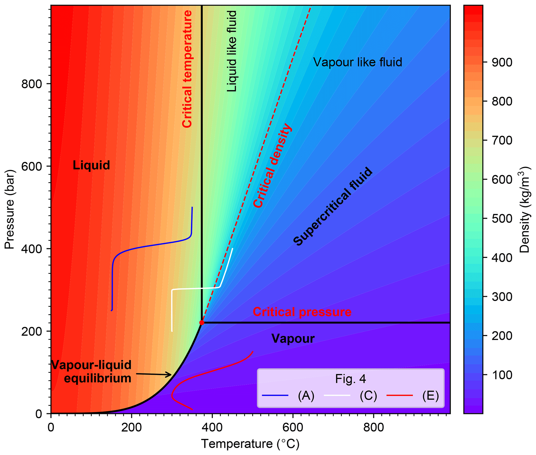
Figure 1 Phase diagram and density of pure water in temperature–pressure space. Red dot denotes supercritical point. The supercritical fluid region is outlined by critical pressure and critical temperature lines and is divided by critical density isoline into liquid-like fluid and vapor-like fluid. Three solid curves in different colors represent pressure-temperature path of 1-D benchmark examples shown in Fig. 4a, c, and e, respectively.

2.3 Time step limitations

To determine the time step, we adopt the limitation related to the Courant number Co, which is defined for compressible fluid as

$$\begin{array}{}\text{(8)}& Co=\underset{\forall \mathrm{cell}}{max}\left({\displaystyle \frac{{\sum }_{\mathrm{F}=\mathrm{1}}^m{\mathit{\varphi }}_{\mathrm{F}}}{\mathrm{2}{\mathit{\rho }}_{\mathrm{f}}{V}_{\mathrm{cell}}}}\right)\mathrm{\Delta }t,\end{array}$$

with m being the number of neighbor faces to a specific cell, ${\mathit{\varphi }}_{\mathrm{F}}={\mathit{\rho }}_{\mathrm{f}}\mathit{U}\cdot {\mathit{S}}_{\mathrm{F}}$ being mass flow through the cell faces, V_cell being volume of the cell, and S_f being area of face F. Then the coefficient for time step change is written as follows:

$$\begin{array}{}\text{(9)}& C_{\mathrm{\Delta }t}={\displaystyle \frac{C{o}_{max}}{Co}}.\end{array}$$

To avoid changes of the time step that are too large, which could lead to numerical instabilities, the time step is defined as follows (Jasak, 1996)

$$\begin{array}{}\text{(10)}& \mathrm{\Delta }t=min(min(C_{\mathrm{\Delta }t},\mathrm{1}+\mathrm{0.1}{C}_{\mathrm{\Delta }t}),\mathrm{1.2})\mathrm{\Delta }{t}_{\mathrm{last}},\end{array}$$

where Δt_last is the time step length of the previous time step. Implementation details can be found in the OpenFOAM documentation and the OpenFOAM source files included by the main source code file HydrothermalSinglePhaseDarcyFoam.C.

2.4 Boundary conditions

To solve the pressure and temperature equations, we have to impose suitable boundary conditions for T and p. The “typical” boundary conditions, e.g., fixed value, fixed gradient, and the mixing of both, are directly inherited from the basic boundary conditions of OpenFOAM. In submarine hydrothermal system modeling,some special adaptations of these basic boundary conditions can also be useful.

The hydrothermal heat flux (q_h) boundary condition is a fixed gradient boundary condition that is often used to approximate heat input from a crustal magma chamber and is commonly used for simulations of mid-ocean ridge hydrothermal systems (e.g., Coumou et al., 2009; Weis et al., 2014). This Neumann boundary condition is called hydrothermalHeatFlux in the toolbox and can be used for the temperature field. Using it, the imposed gradient of temperature can be expressed as

$$\begin{array}{}\text{(11)}& \mathit{n}\cdot \mathrm{\nabla }T=-\mathit{n}\cdot {\displaystyle \frac{{\mathit{q}}_{\mathrm{h}}}{k_{\mathrm{r}}}},\end{array}$$

where n denotes the normal vector of the face boundary. In addition, we implement two options for heat flux distribution. Using the keyword shape allows for modifying the functional form of the heat flux boundary. The available options are fixed, gaussian2d, gaussian3d. The default option is fixed, and if gaussian2d or gaussian3d is specified, the Gaussian shape (Eq. 12) related parameters (qmin, qmax, c, x0 and/or z0) have to be specified (see Sect. 5.3).

$$\begin{array}{}\text{(12)}& q_h(x,z)=q_{min}+(q_{max}-q_{min})e^{-\frac{(x-x_{\mathrm{0}}{)}^{\mathrm{2}}+(y-z_{\mathrm{0}}{)}^{\mathrm{2}}}{\mathrm{2}{c}^{\mathrm{2}}}}\end{array}$$

A similar boundary condition called hydrothermalMassFluxPressure is defined for the pressure field to prescribe a mass influx into the modeling domain (ϕ_m=ρ_fU). The corresponding gradient of the pressure field can be derived from Darcy's law (Eq. 1)

$$\begin{array}{}\text{(13)}& \mathit{n}\cdot \mathrm{\nabla }p=\mathit{n}\cdot \left({\mathit{\rho }}_{\mathrm{f}}\mathit{g}-{\displaystyle \frac{{\mathit{\mu }}_{\mathrm{f}}}{k}}\mathit{U}\right)={\displaystyle \frac{{\mathit{\mu }}_{\mathrm{f}}}{{\mathit{\rho }}_{\mathrm{f}}k}}\mathit{n}\cdot ({\mathit{\varphi }}_{\mathrm{g}}-{\mathit{\varphi }}_{\mathrm{m}}).\end{array}$$

Where ϕ_m and ϕ_g denote mass flux and gravity-related flux, respectively. Further, we define another Neumann boundary condition (named noFlux) for the pressure field for impermeable boundaries, which is a special case of HydrothermalMassFluxPressure when ϕ_m=0. In addition, a Dirichlet boundary condition (named submarinePressure) for the pressure field is defined to describe hydrostatic pressure at the seafloor boundary due to bathymetric relief. Another commonly used boundary condition on hydrothermal venting boundary (e.g., seafloor) is OpenFOAM's inletOutlet boundary condition, which allows for the setting of a constant temperature for inflow and zero heat flux for outflow nodes – this type of boundary condition is often used to mimic free venting at the seafloor.

2.5 Fluid properties and equation-of-state

Numerical solutions of hydrothermal flow are known to strongly depend on the used thermodynamic properties of the simulated fluid. A series of studies using realistic thermodynamic properties of pure and salt water, rather than making a Boussinesq approximation or using linearized properties, have shown that realistic results depend critically on using a realistic EOS (Jupp and Schultz, 2000; Hasenclever et al., 2014; Driesner, 2010; Carpio and Braack, 2012). Note that we here do not address any issues related to using pure versus saltwater EOSs, as outlined in the introduction. We use an EOS for pure water based on the IAPWS-IF97 parameterization and have created a corresponding OpenFOAM thermo-physical model in a single phase regime. The phase diagram is shown in Fig. 1.

Figure 2 Schematic of the sequential algorithm.

2.6 Solution algorithm

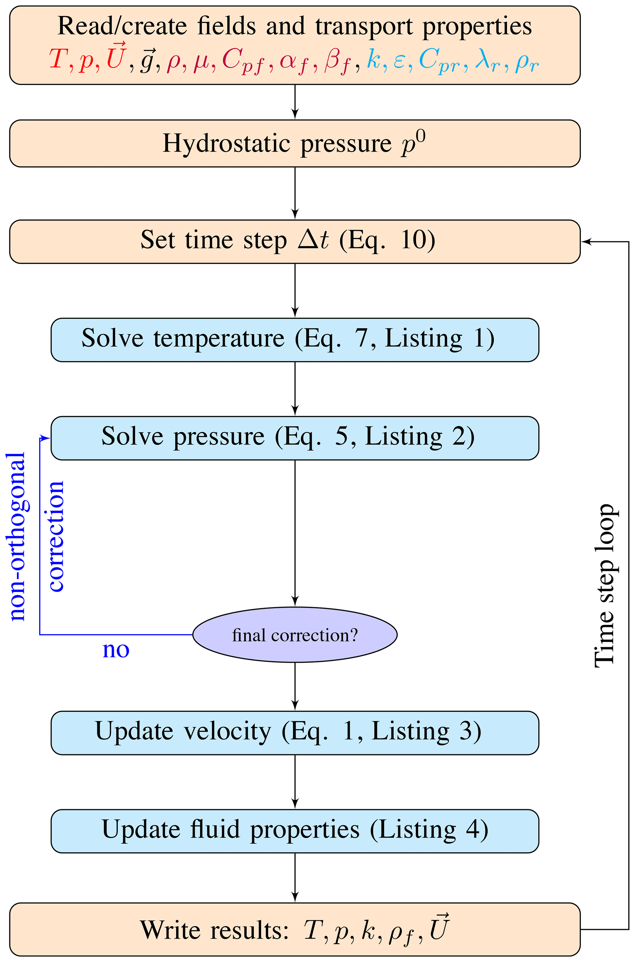
The governing equations of pressure and temperature are solved in a sequential approach. The primary variables (pressure and temperature) and transport properties (such as permeability, porosity, etc.) have to be initialized before the time loop, and then the initial Darcy velocity and thermodynamic properties of fluid can be updated according to the temperature and pressure fields. The main computational sequence for a single time step is described below and sketched in Fig. 2.

Listing 1 Implementation of temperature Eq. (7) with OpenFOAM (in EEqn.H).

Listing 2 Implementation of pressure Eq. (5) with OpenFOAM (in pEqn.H).

1. The time step size Δtⁿ⁺¹ is calculated from the condition related to the Courant number (Eq. 8).

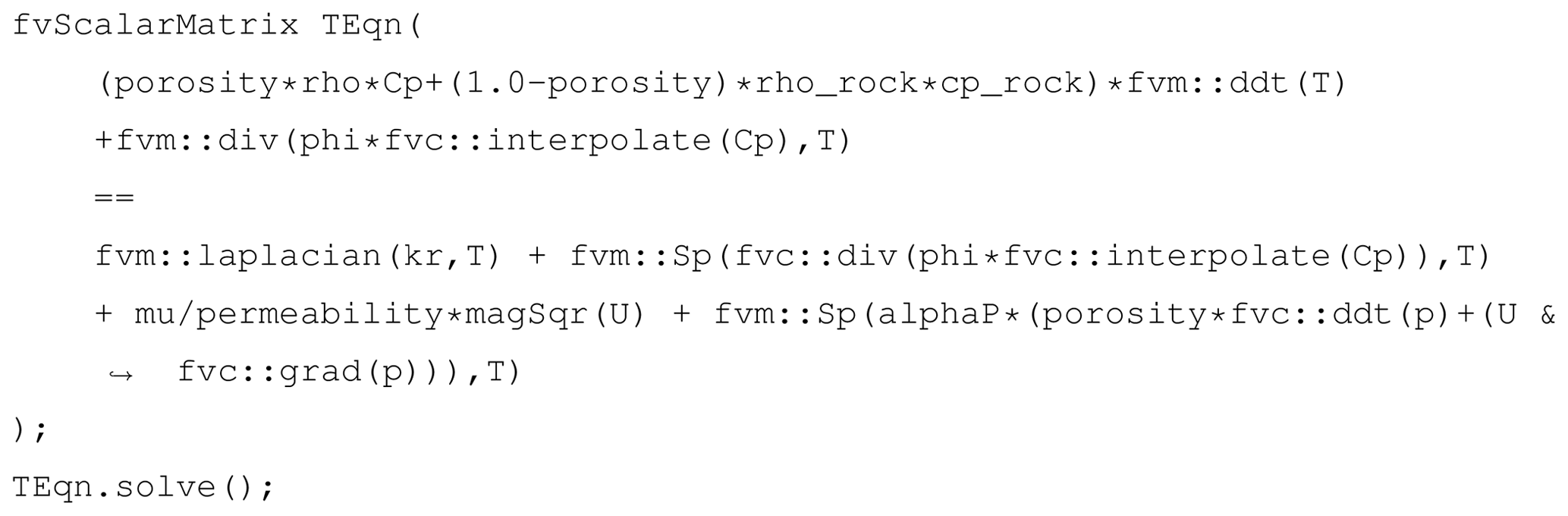
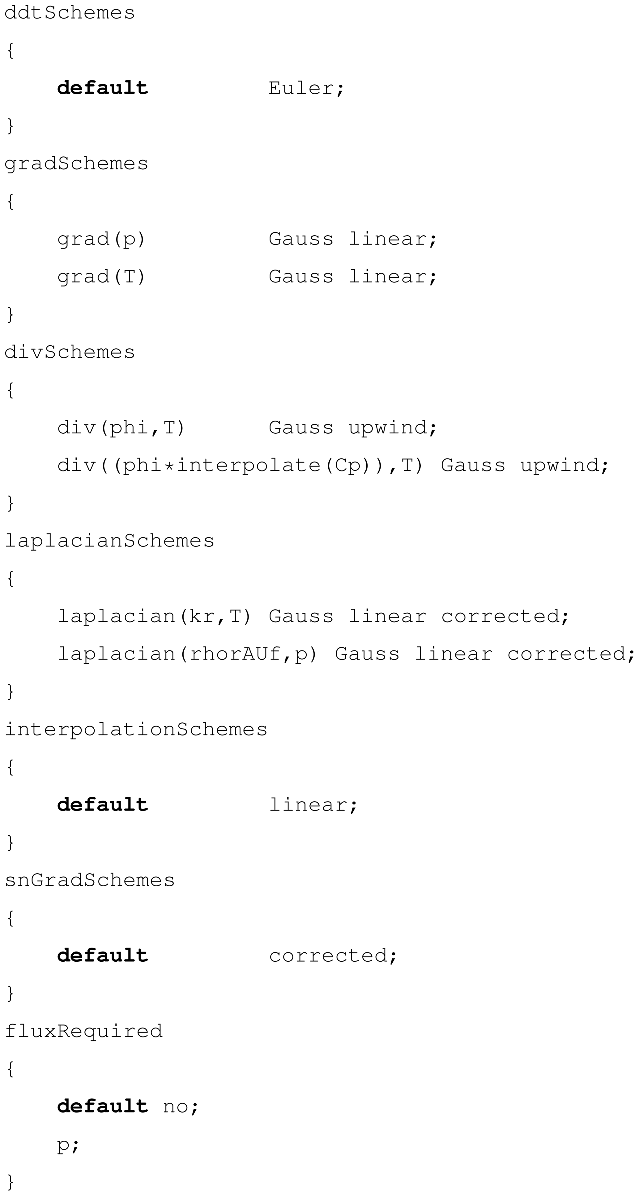
2. Temperature field Tⁿ⁺¹ is implicitly computed by solving the energy conservation equation (Eq. 7). The syntax of a partial differential equation (PDE) in OpenFOAM is very close to mathematical formulation, and a code snippet of the temperature Eq. (7) implementation is shown in Listing 1. All variable symbols, names, and OpenFOAM types (classes) are shown in Table 1. The transient term $\partial T/\partial t$ can be implicitly discretized using the OpenFOAM operator fvm::ddt(T) with the discretization scheme (e.g., Euler scheme) being specified under the keyword ddtSchemes in the system/fvSchemes dictionary file (see Listing A1). The divergence term, Laplace term, and source term are implicitly discretized using fvm::div, fvm::laplacian and fvm::Sp operators. The last term on the right-hand side is explicitly calculated using known field values from the current or previous time step; the corresponding time derivative and gradient can be programmed using fvc::ddt and fvc::grad, respectively.

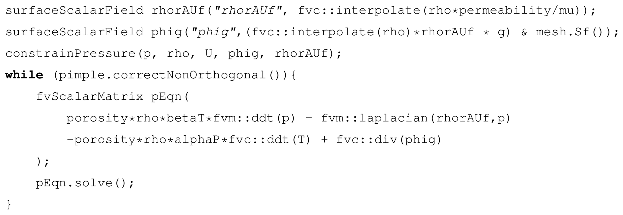
3. The pressure field pⁿ⁺¹ is implicitly computed by solving the pressure equation (Eq. 5), the code snippet is shown in Listing 2. The temperature temporal term and divergence of ϕ_g on the right-hand side are evaluated explicitly by using fvc::ddt(T) and fvc::div(phig) (see line 7 in Listing 2). Although pressure boundary conditions are customized by flux directly (see Sect. 2.4), in order to specify pressure boundary conditions through velocity boundary conditions, e.g., OpenFOAM's fixedFluxPressure boundary condition, the OpenFOAM function of constrainPressure has to be called before solving the pressure equation (see line 3 in Listing 2). For non-orthogonal mesh, a non-orthogonal correction algorithm (line 4 in Listing 2) is commonly adopted to improve accuracy for gradient computation. The number of non-orthogonal corrections is specified by the nNonOrthogonalCorrectors key in the PIMPLE sub-dictionary in the system/fvSolution file.

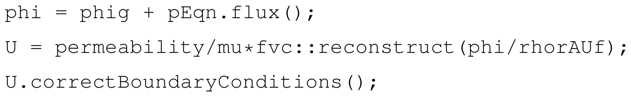
4. The velocity field is calculated explicitly using the latest pressure field based on Darcy's law (Eq. 1). Instead of calculating the velocity directly, we implement an indirect approach based on OpenFOAM's function fvc::reconstruct to reconstruct the velocity field from the computed mass flux (see Listing 3), which performs under higher numerical stability and benefits from the flux conservation characteristics of the finite-volume method. In addition, the boundary conditions of the velocity field have to be updated (line 3 in Listing 3) if OpenFOAM's fixedFluxPressure boundary condition is applied for the pressure field.

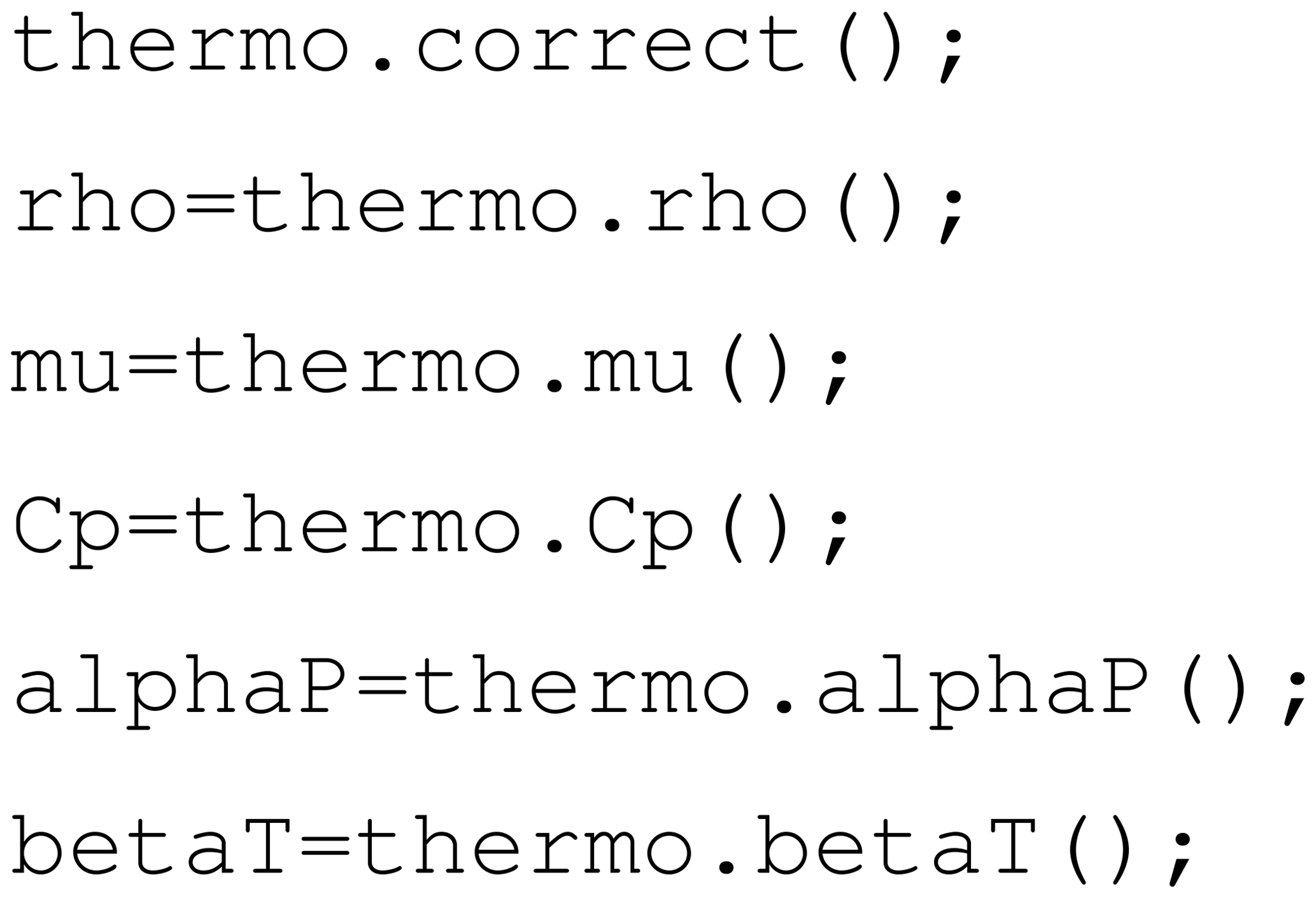
5. Thermodynamic properties of fluid are updated by the thermo-physical model after solving the temperature and pressure field. The implementation code snippet is shown in Listing 4, in which thermo.correct() is used to update the temperature and pressure value for all the calculating nodes. Then the thermodynamic properties of the fluid, for example density (ρ) at each node, are calculated based on IAPWS-IF97 (see line 2–6 in Listing 4).

Listing 3 Implementation of Darcy velocity calculation with OpenFOAM (in pEqn.H).

Listing 4 Update of fluid thermodynamic properties (in updateProps.H).

2.7 Numerical schemes

Since the numerical evaluation of the divergence and gradient terms in the governing equations has great influence on heat and mass transfer, a suitable solution strategy regarding discretization and linear solver schemes needs to be chosen to ensure accuracy, robustness, and stability. In the presented solver HydrothermalSinglePhaseDarcyFoam, the discretization and interpolation scheme of the primary fields (T,p) can be defined in the simulation configuration files. In the following benchmark tests (Sect. 5), the advective discretization scheme is set to upwind to ensure consistency with HYDROTHERM. It should be noted that all of the basic numerical schemes of OpenFOAM are also valid for HydrothermalSinglePhaseDarcyFoam solver.

3 Description of toolbox components

The organization of the HydrothermalFoam toolbox is shown in Fig. 3. The toolbox contains five parts: a HydrothermalFoam solver, thermo-physical models, boundary conditions, cookbooks, and a manual.

• HydrothermalSinglePhaseDarcyFoam. This block compiles the solver (an executable file) that solves the seafloor hydrothermal convection equations described in Sect. 2.1. It can be used to simulate single-phase hydrothermal circulation in an isotropic porous medium.

• ThermoModels. This block compiles the libHydroThermoPhysicalModels library, containing the EOS of pure water, which is used to formulate the used thermo-physical model; see Sect. 2.5.

• BoundaryConditions. This block compiles libHydrothermalBoundaryConditions library, containing four customized boundary conditions explained in Sect. 2.4. The example usage of each boundary condition can be found in the cookbooks and manual in the following GitLab repository (https://gitlab.com/gmdpapers/hydrothermalfoam, last access: 21 December 2020).

• benchmarks. This block contains the input files of all the benchmark tests (see Sect. 5) presented in this paper.

• cookbooks. This block contains some example cases of parallel computing, user-defined boundary conditions, and post-processing.

• manual. The manual presents detailed usage and all the numerical examples in cookbooks.

Figure 3 Structure and components of the HydrothermalFoam toolbox.

4 Installation

We provided two options for installation: one is building from source and the other is using a pre-compiled docker image.

4.1 Building from source code

4.1.1 OpenFOAM

The HydrothermalFoam v1.0 is developed based on https://github.com/OpenFOAM/OpenFOAM-7, which can be installed according to the installation instructions (https://openfoam.org/download/, last access: 21 December 2020) given by the development team at https://openfoam.org/download/7-ubuntu/ (last access: 21 December 2020), https://openfoam.org/download/7-linux/ (last access: 21 December 2020), https://openfoam.org/download/7-macos/ (last access: 21 December 2020), and https://openfoam.org/download/windows-10/ (last access: 21 December 2020) for each platform.

4.1.2  HydrothermalFoam

Once OpenFOAM is built successfully, the source code of HydrothermalFoam can be downloaded from https://doi.org/10.5281/zenodo.3755647 (Guo and Rüpke, 2020). The directory structure and components of HydrothermalFoam are shown in Fig. 3 and the components can be built following the three steps given below.

1. Build a freesteam-2.1 library. The freesteam project is constructed by https://scons.org (last access: 21 December 2020), which is an open-source software construction tool dependent on https://www.python.org/downloads/release/python-272/ (last access: 21 December 2020), and based on https://www.gnu.org/software/gsl/doc/html/ (last access: 21 December 2020) (GNU Scientific Library, GSL). Therefore, Python 2, SCons, and GSL have to be installed first, followed by changing the directory to freesteam-2.1 in the HydrothermalFoam source code and type command of scons install to compile the freesteam library.

2. Build libraries of customized boundary conditions and thermo-physical model. Change directory to libraries and type command of ./Allmake to compile the libraries.

3. Build solver. Change directory to HydrothermalSinglePhaseDarcyFoam and type command of wmake to compile the solver.

All the library files and executable application (solver) file will be generated in directories defined by OpenFOAM's path variables of FOAM_USER_LIBBIN and FOAM_USER_APPBIN, respectively.

4.2 Pre-compiled docker image

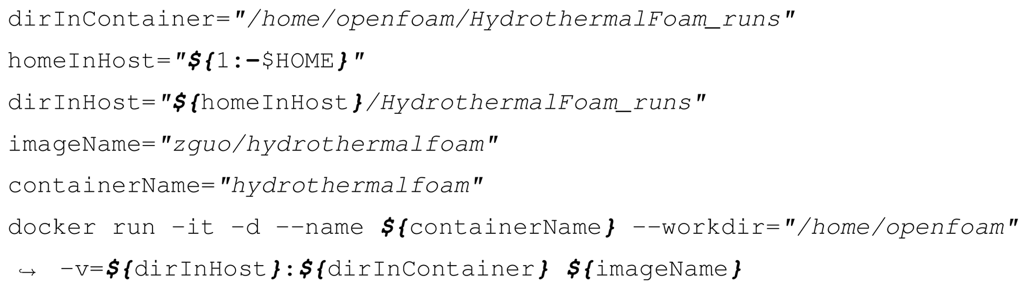
In order to use all the tools directly without any compiling and development skills, we have published a pre-compiled Docker^® image in a repository at https://hub.docker.com/repository/docker/zguo/hydrothermalfoam (last access: 21 December 2020). The docker image can be used on any operation system (e.g., Windows, Mac OS, and Linux) to run HydrothermalFoam cases following the five steps below.

1. Install Docker, then open Docker and keep it running.

2. Pull the docker image by using command of docker pull zguo/hydrothermalfoam in the shell terminal, e.g., bash shell in Mac OS or PowerShell in Windows system.

3. Install a container from the docker image by running a shell script, e.g., Unix shell script, shown in Listing 5. The directory named HydrothermalFoam_runs is a shared folder between the container and host machine.

4. Start the container by running the command docker start hydrothermalfoam.

5. Attach the container by running the command docker attach hydrothermalfoam. The user is now in a Ubuntu Linux environment with pre-compiled HydrothermalFoam tools that are located at the directory  /HydrothermalFoam. We recommend that the user runs HydrothermalFoam cases in the directory HydrothermalFoam_runs in the container, then the results will be synchronized in the shared directory in the host and thus can be visualized by ParaView^®, Tecplot^®, or other software.

Following above five steps, one can run HydrothermalFoam tools in the current shell terminal. The following links can be found in the Docker Hub repository: https://hub.docker.com/repository/docker/zguo/hydrothermalfoam (last access: 21 December 2020) and https://youtu.be/6czcxC90gp0 (last access: 21 December 2020) (5 min tutorial video).

Listing 5 Script for installing a container from the HydrothermalFoam docker image.

4.3 Run the first case of HydrothermalFoam

The basic directory structure for a HydrothermalFoam case that contains the mandatory files to run an application is shown in Fig. 4. There is a bash script file named run.sh in every HydrothermalFoam case provided by this paper. A HydrothermalFoam case can be run by executing ./run.sh. In addition, we provide a 5 min quick start tutorial video (https://youtu.be/6czcxC90gp0, last access: 21 December 2020) to run the first case of HydrothermalFoam in Docker.

Figure 4 Case directory structure of the HydrothermalFoam toolbox.

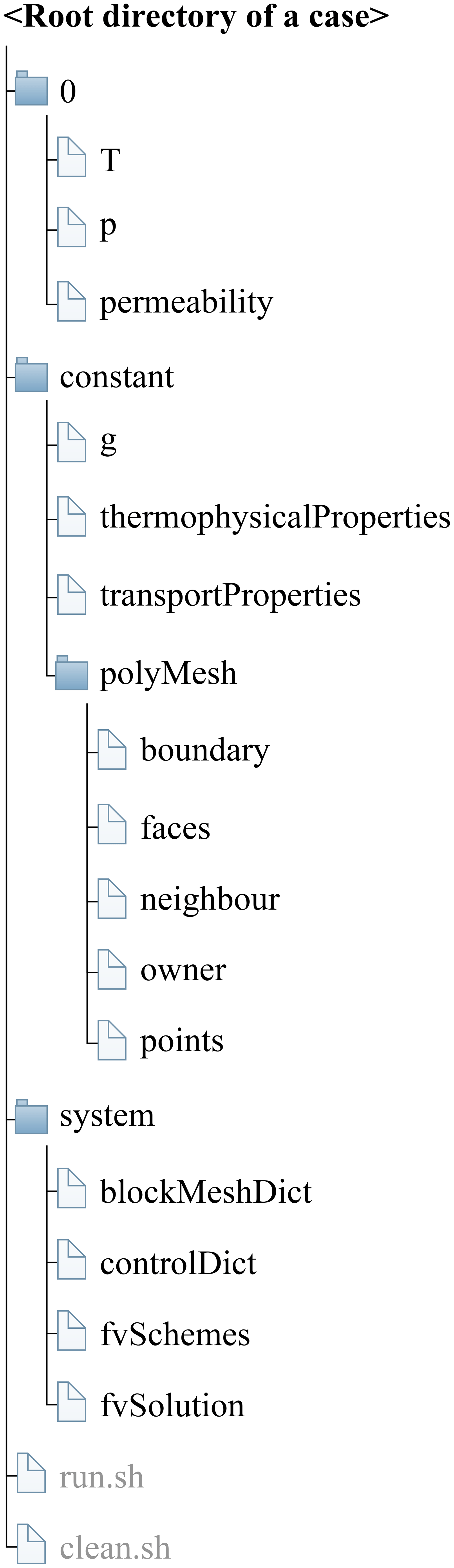
4.3.1 Mesh generation

The mesh information containing boundary patches definitions, cell face indices, and connections is located in the polyMesh subdirectory in the constant directory in a specific case folder (Fig. 4). All the OpenFOAM mesh generation approaches can be applied to HydrothermalFoam as well. For example, blockMesh generates a simple mesh defined by the blockMeshDict dictionary file in the system directory, and gmshToFoam transforms a mesh file generated by https://gmsh.info (last access: 21 December 2020) (Geuzaine and Remacle, 2009) to polyMesh.

4.3.2 Input field data

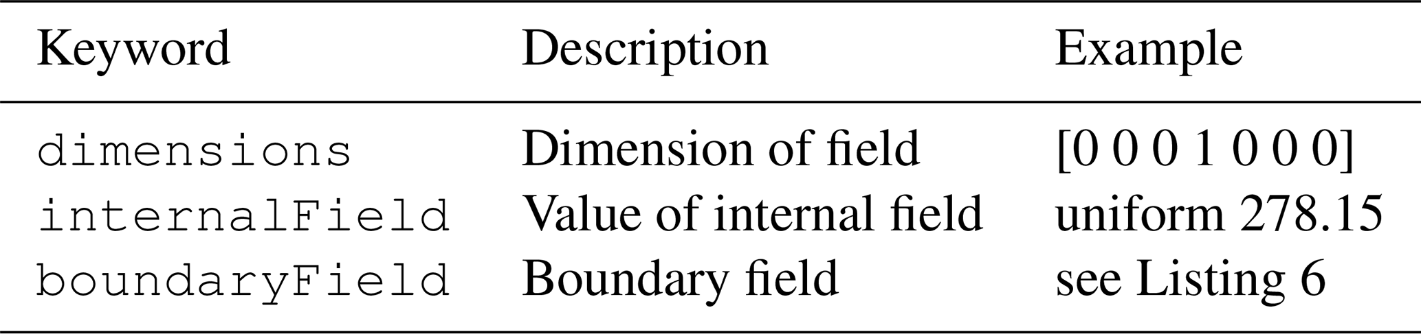
Much of the input–output data in HydrothermalFoam are fields, e.g., temperature or pressure data, that are read from and written into the time directories. For example, the initial time directory is commonly named 0 (see Fig. 4). HydorthermalFoam writes field data as dictionary files using keyword entries described in Table 2.

Table 2 Main keywords used in field dictionary files.

The required input field data of HydrothermalFoam are temperature, pressure, and permeability. Each kind of input field data begins with an entry for its dimensions, which is expressed by a vector of seven basic SI units (International System of Units) in the following order: kg, m, s, K, mol, A, and cd. The file names are the same as the variable names shown in Table 1. Following this is the internalField, described in one of the following ways.

1. Uniform field. A single value is assigned to all elements within the field, taking the form:
   internalField uniform <entry>;

2. Nonuniform field. Each field element is assigned a unique value from a list, taking the form:
   internalField nonuniform <List>;
   The nonuniform list of an internal field, e.g., permeability, can be specified in different mesh regions by using setFields transform setFieldsDict in the system directory (see the https://gitlab.com/gmdpapers/hydrothermalfoam/-/tree/master/benchmarks/HydrothermalFoam/3d/Heterogeneous (last access: 21 December 2020) benchmark example described in Sect. 5.3.2).

Listing 6 Example dictionary file for temperature field T.

The boundaryField is a dictionary containing a set of entries whose names are listed in the polyMesh/boundary file for each boundary patch. The compulsory entry, type, describes the boundary condition specified for the field. Aside from the OpenFOAM internal basic boundary condition types of fixedValue, zeroGradient, codedFixedValue, etc., the customized boundary condition types, e.g., noFlux for pressure and HydrothermalHeatFlux for temperature, are described in Sect. 2.4. An example set of field dictionary entries for temperature T are shown in Listing 6. While a boundary condition for permeability is not mathematically required, its internal OpenFOAM data type requires a corresponding boundaryField dictionary with specified boundary conditions. Therefore, we suggest that the type entry of all boundary patches for permeability field should be always set to zeroGradient.

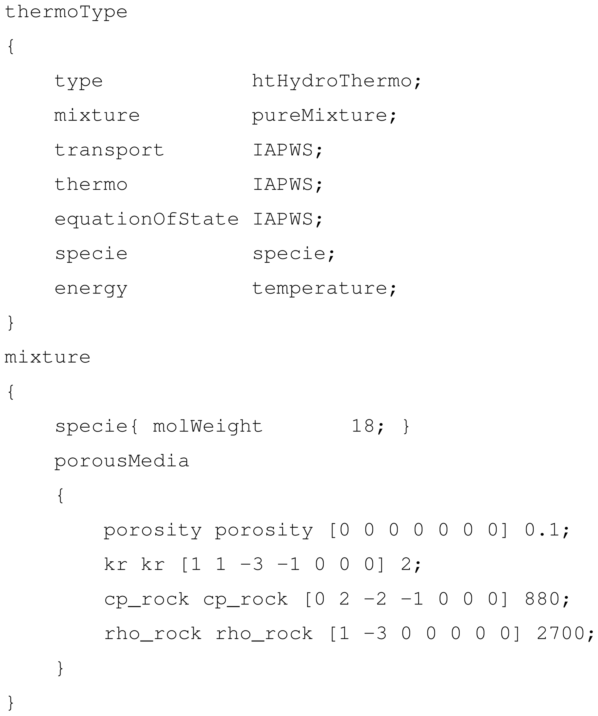
4.3.3 Thermo-physical model

The thermophysicalProperties is a compulsory file in the constant directory, it contains keywords (Listing 7) of the newly defined thermo-physical model for water, which is described in Sect. 2.5 and contains constant properties of rock, e.g., porosity and density. It should be noted that porosity is implemented as volScalarField type just like permeability. It means that user can define a porosity field in the modeling domain. If the porosity file does not exist in the start time folder, e.g., the 0 folder, the solver will initialize the porosity field by using the constant porosity value specified in the porousMedia sub-dictionary in the constant/thermophysicalProperties file.

Listing 7 thermophysicalProperties file.

4.3.4 Discretized schemes and solution control

The discretization schemes for primary variables in the PDEs (partial difference equations) and solver for linear equations are specified in fvSchemes and fvSolution files in the system directory, respectively. According to the implementation of temperature equation (Listing 1) and pressure equation (Listing 2), we have to specify discretization schemes for the transient terms, Laplace terms, and gradient and divergence terms, which are shown in Listing A1. A example of solver, preconditioner, and tolerance settings for linear equations of temperature and pressure fields are shown in Listing A2. We recommend keeping these two files the same for different cases unless one attempts to try different options available in OpenFOAM.

5 Benchmark tests

We have conducted a number of one-dimensional (1-D), two-dimensional (2-D), and three-dimensional benchmark tests and compared the results to other established software packages to validate HydrothermalFoam and to highlight some of its advantages. The reference software we used is version 3.1 of HYDROTHERM, a simulation tool developed and maintained by the US Geological Survey (USGS), which can be downloaded from the internet (https://volcanoes.usgs.gov/software/hydrotherm/index.html, last access: 21 December 2020) for free. All the parameters used in the 1-D and 2-D examples are taken from Weis et al. (2014), who presented a sequence of well-defined and highly useful benchmarks designed to test code performance within different key thermodynamic fluid states. In those benchmarks the transport properties and rock properties are constant and uniform (values are also listed in Table 1); an isotropic permeability of $k={\mathrm{10}}^{-\mathrm{15}}$ m², a porosity of ε=0.1, a heat capacity of C_pr=880 J/(kg ^∘C), a thermal conductivity of k_r=2 W/(m ^∘C), and a rock density of ρ_r=2700 kg/m³ are used in all simulations below.

5.1 One-dimensional simulations

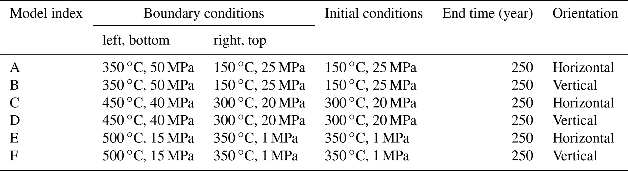
We conducted six 1-D simulations to test the code performance along the three p–T paths in the phase diagram of pure water shown in Fig. 1. These runs are designed with constant pressure and temperature conditions on both ends of a domain with 2 km length and 10 m grid spacing. The boundary conditions and initial conditions of each 1-D test are listed in Table 2. For comparison, we use the same parameters for the HYDROTHERM simulations. The computational domain is oriented horizontally (model index are A, C, E) without gravity and vertically (model index are B, D, F) with gravity to evaluate gravitational effects on fluid flow. All input files can be found in the https://gitlab.com/gmdpapers/hydrothermalfoam/-/tree/master/benchmarks/HydrothermalFoam/1d (last access: 21 December 2020) and https://gitlab.com/gmdpapers/hydrothermalfoam/-/tree/master/benchmarks/USGS_HYDROTHERMAL/1d (last access: 21 December 2020) directories.

Table 3 Model parameters of 1-D benchmark examples.

Simulation results of the six 1-D examples are shown in Fig. 5. The example runs A and B describe invasion of a hot fluid into an initially colder domain and the fluids stay in single-phase liquid state. The thermal front moves from the start point (left and bottom for the horizontal and vertical example, respectively) towards the end point. As the vertical flow is opposing gravity, the flow is about 3 times slower. The fluids remain at pressures beyond the critical end point of pure water and therefore in the single-phase regime. Results calculated by HYDROTHERM and HydrothermalFoam are almost identical. In Examples A (horizontal) and B (vertical), the fluid remains in a liquid-like state, while in the examples C (horizontal) and D (vertical) the fluid flows along the pressure gradient from a cold liquid-like state to a hot vapor-like state. In C and D the fluids moves about 2 times faster than in A and B, resulting in a sharper thermal front. The sharpness of this front is, unfortunately, often affected by the numerical scheme (e.g., mesh geometry, upwinding scheme, and advection scheme). In fact, OpenFOAM seems to cope a bit better with resolving the sharpness of the front despite also using an upwind advection scheme. Benchmarks E and F explore sub-critical vapor flow. The results of horizontal and vertical flow look very similar because the density of single-phase vapor fluid is very low and thus the gravitational effects are relatively small with respect to the liquid cases. The results of HydrothermalFoam have a good agreement with that of HYDROTHERM for single-phase vapor flow.

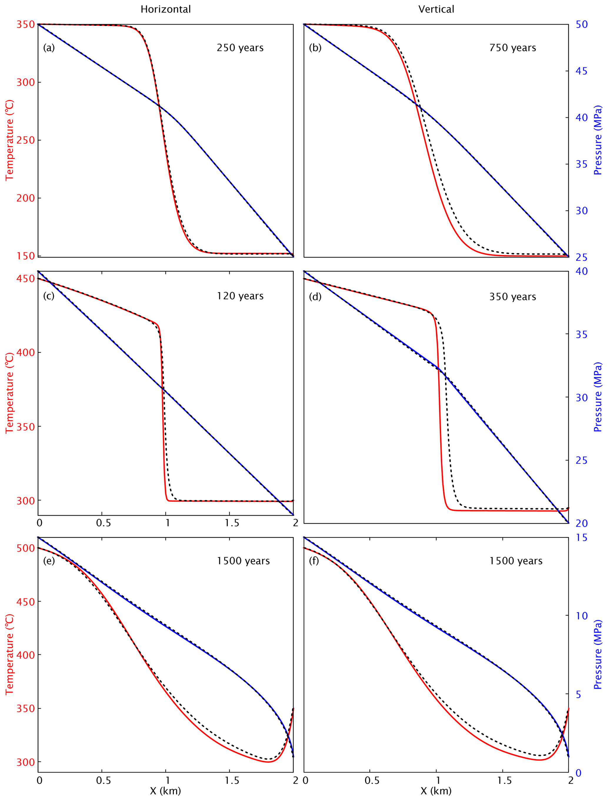
Figure 5 Snapshots of one-dimensional benchmark examples in horizontal (a, c, e) and vertical (b, d, f) orientation. Results (temperature in red and pressure in blue) of HydrothermalFoam and HYDROTHERM are plotted as solid lines and dashed lines, respectively.

5.2 Two-dimensional simulations

The two-dimensional models are performed on a rectangular domain with a length of 9 km in the x direction and 3 km in the y direction (Fig. 6), loosely representative of a vertical section through the upper oceanic crust with uniform permeability. The top boundary represents the seafloor and is kept at a constant pressure of 30 MPa, which is equivalent to about 3 km water depth, and a constant temperature of 5 ^∘C. At the bottom, a constant heat flux of Q_b=0.05 W/m² is applied. Further, we assume a magmatic heat source with constant heat flux of Q_m=5 W/m² extending 1 km wide along the x direction located at the center of the bottom boundary (shown in red line in Fig. 6).

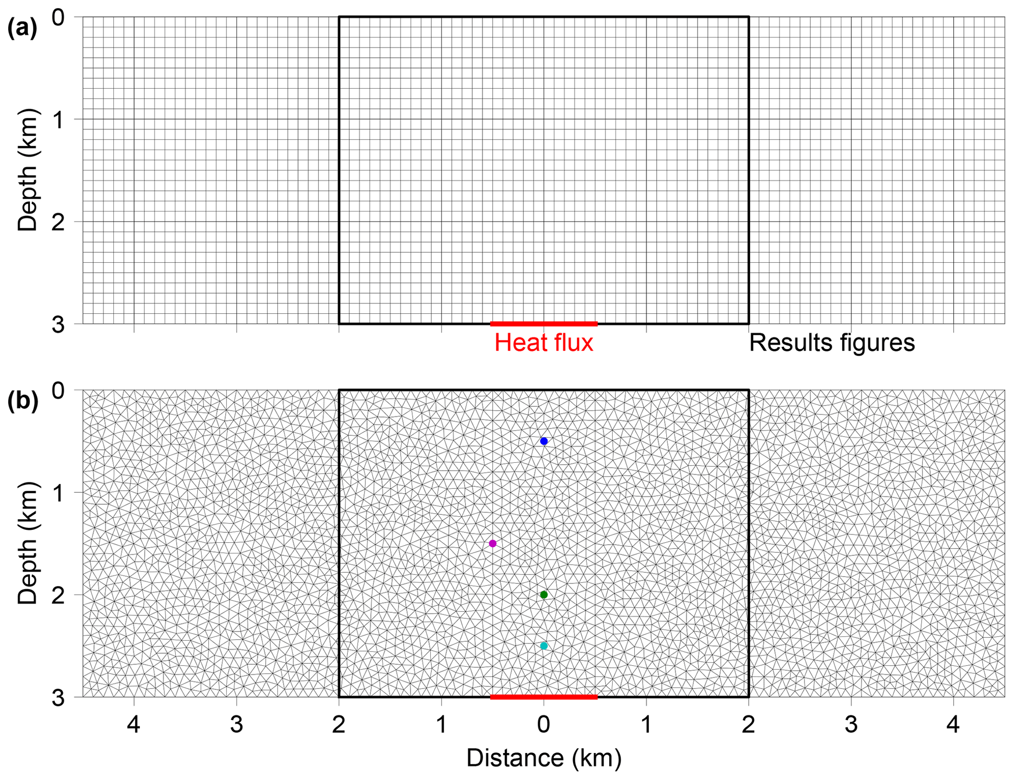
Figure 6 Mesh and model configuration of the two-dimensional examples. (a) The grid for HYDROTHERM has to be set to a uniform regular mesh with resolution of 100 m and a total number of 2700 elements. (b) HydrothermalFoam uses an unstructured mesh with 7074 triangular elements and an edge length in the range of 60–142 m. Red lines on the bottom boundaries denotes heat flux boundary condition for temperature.

The simulation results are shown in Fig. 7. Fluid pressure and temperature calculated by HydrothermalFoam and HYDROTHERM agree very well. The evolution of the hydrothermal plume is summarized in Fig. 7a–c. A hot plume is forming at the base and rises upwards after 5 kyr (Fig. 7a) reaching the seafloor at 15 kyr (Fig. 7b). After 50 kyr, a quasi-steady hydrothermal circulation cell is established (Fig. 7c). The results of HydrothermalFoam and HYDROTHERM are again very similar. All input files can be found in the following directories: https://gitlab.com/gmdpapers/hydrothermalfoam/-/tree/master/benchmarks/HydrothermalFoam/2d (last access: 21 December 2020) and https://gitlab.com/gmdpapers/hydrothermalfoam/-/tree/master/benchmarks/USGS_HYDROTHERMAL/2d (last access: 21 December 2020).

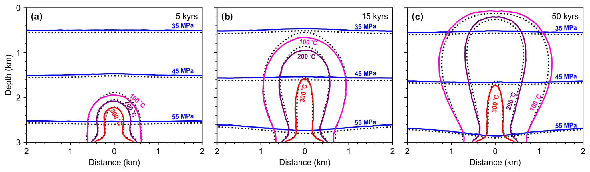
Figure 7 Snapshots of two-dimensional examples. Contour lines for fluid pressure (blue) and temperature (red) calculated from HydrothermalFoam are plotted as solid lines and those from HYDROTHERM are plotted as dotted lines (black). The visualization window is shown by the black box in Fig. 6

5.3 Three-dimensional simulation

5.3.1 Homogeneous model

Similar to the two-dimensional model in Sect. 5.2, the three-dimensional models are performed on a cubic domain with a length of 9 km in both the x direction and the z direction and 3 km in y direction (vertical direction). Note that the vertical coordinate in HydrothermalFoam or OpenFOAM is y rather than z. It can be imagined as representing a three-dimensional section of oceanic crust with uniform permeability. The top boundary is the seafloor and is kept at a constant pressure of 30 MPa and a constant temperature of 5 ^∘C. At the bottom boundary, a zero mass flux is applied for pressure, and a constant Gaussian-shaped heat flux (see Eq. 12) is applied for temperature. The corresponding parameters in Eq. (12) are $x_{\mathrm{0}}=\mathrm{0},z_{\mathrm{0}}=\mathrm{0},q_{max}=\mathrm{5}$ W/m², $q_{min}=\mathrm{0.05}$ W/m², and c=500. All input files can be found in the 3d/Homogeneous directory in benchmarks/HydrothermalFoam and benchmarks/USGS_HYDROTHERMAL directories, respectively.

The simulation results at 50 kyr are shown in Fig. 8. Vertical slices at x=0 km and x=0.5 km, and horizontal slices at z=0.5 km and z=2.5 km are shown in Fig. 8a–d. Fluid pressure (blue contours) and the temperature field calculated by HydrothermalFoam and HYDROTHERM (dashed contours) agree very well, and the results of the central vertical slice are very close to two-dimensional model results shown in Fig. 7c. Three-dimensional flow path and isothermal surfaces of 300, 200, and 100 ^∘C are shown in Fig. 8e.

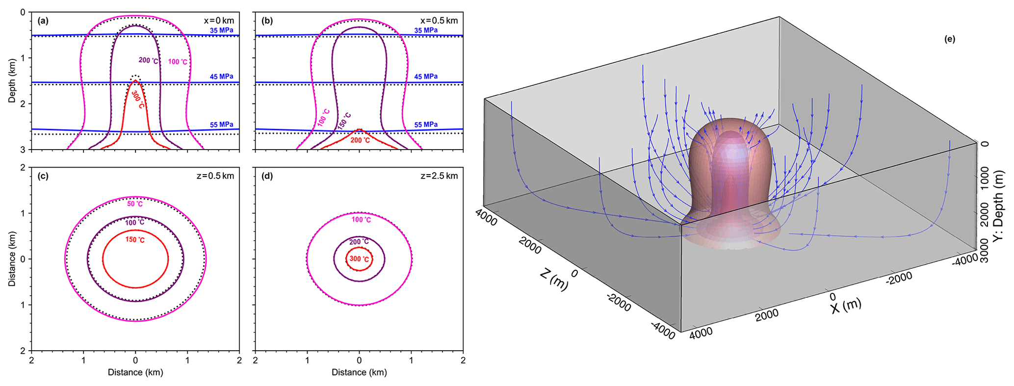
Figure 8 Snapshots of three-dimensional model results. Contour lines for fluid pressure (blue) and temperature calculated from HydrothermalFoam are plotted as solid lines, and those from HYDROTHERM are plotted as dotted black lines. Panels (a) and (b) show pressure and temperature contours on vertical slices, and panels (c) and (d) show temperature contours on horizontal slices. Panel (e) shows three-dimensional isothermal surfaces and stream lines.

5.3.2 Heterogeneous model

The heterogeneous model with two-layer permeability structure is modified from the homogeneous model described in Sect. 5.3.1. Permeability values of two layers are $k_{\mathrm{1}}={\mathrm{10}}^{-\mathrm{14}}$ m² and $k_{\mathrm{2}}={\mathrm{10}}^{-\mathrm{15}}$ m², respectively (see Fig. 9a). The thickness of first layer is 1.1 km, and the other parameters are the same as the homogeneous model. All input files can be found in the 3d/Heterogeneous directory in benchmarks/HydrothermalFoam and benchmarks/USGS_HYDROTHERMAL directories, respectively. The simulation results at 50 kyr are shown in Fig. 9. Vertical slices at x=0 km and x=0.5 km and horizontal slices at z=0.5 km and z=2.5 km are shown in Fig. 9a–d. The higher permeability in the upper layer results in mixing with colder ambient fluids and focusing of the upflow zone. Three-dimensional isothermal surfaces of 300, 200, and 100 ^∘C are shown in Fig. 9e.

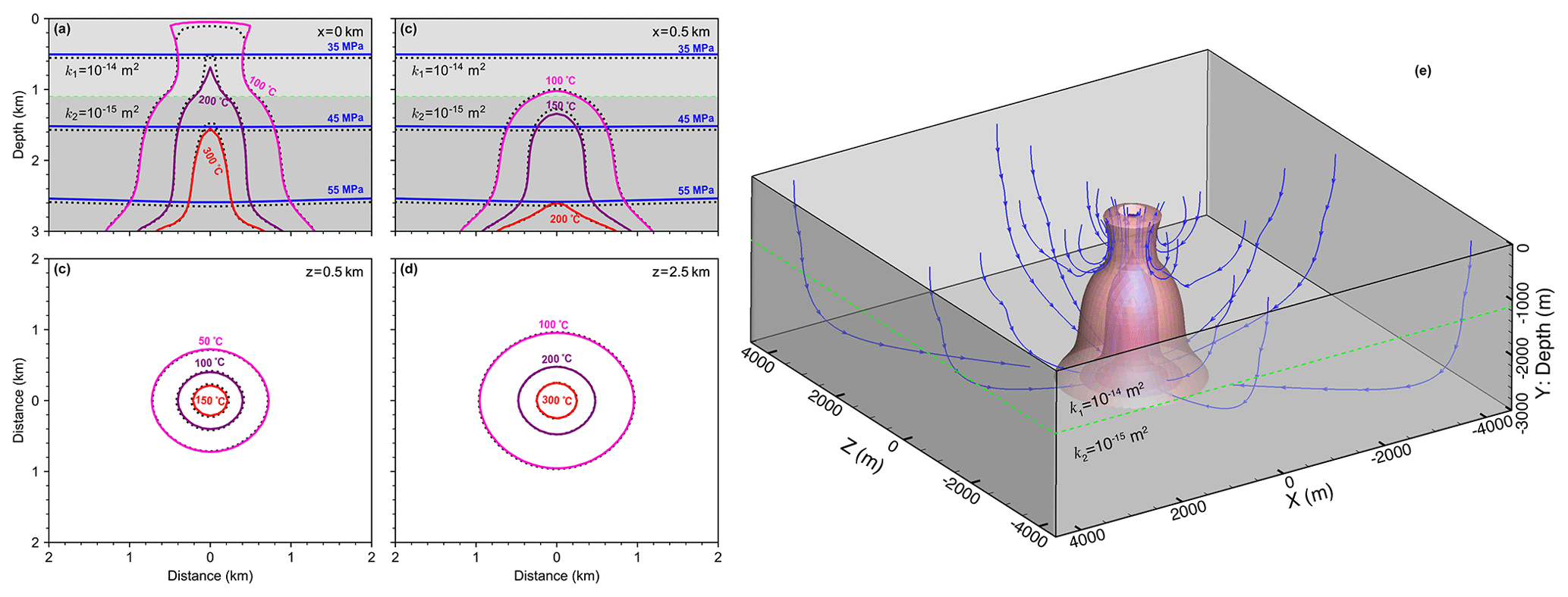
Figure 9 Results of three-dimensional model with two-layer permeability structure. Two layers are separated by the dashed green line. Contour lines for fluid pressure (blue) and temperature calculated from HydrothermalFoam are plotted as solid lines, and that from HYDROTHERM are plotted as dotted black lines. Panels (a) and (b) show pressure and temperature contours on vertical slices, panels (c) and (d) show temperature contours on horizontal slices. Panel (e) shows three-dimensional isothermal surfaces and stream lines.

5.4 Cookbooks

In addition to the presented benchmarks, we have added a number of cookbooks to the code repositories that can be used as starting points for more complex models. These include simple 2-D and 3-D box models, 2-D single-pass loop models, and time-dependent permeability models. They also include examples of how to use more complex meshes generated by Gmsh (Geuzaine and Remacle, 2009). We intend to add additional cookbooks in the future and hope to receive contributions from users of HydrothermalFoam.

6 Conclusions

We have presented a toolbox for simulating flow in submarine hydrothermal circulation systems. Being based on the widely used fluid-dynamic simulation platform OpenFOAM, the toolbox provides the user with robust parallelized 3-D solvers and a whole suite of pre- and post-processing tools. The toolbox is meant to provide the interdisciplinary submarine hydrothermal systems community with an accessible and easy-to-use open-source platform for testing ideas on how hydrothermal systems “work”. The benchmark tests have shown that model matches previously published models and that the cookbooks provide the user with starting points for building more sophisticated models. By following an open-source approach and by providing extensive code documentation, we hope that the presented model will facilitate integrative studies that combine models with data to better assess the role of submarine hydrothermalism in the Earth system.

Appendix A: Key code snippets

Listing A1 Example of fvSchemes file.

Listing A2 Example of fvSolution file.