the Creative Commons Attribution 4.0 License.
the Creative Commons Attribution 4.0 License.
 | 22 Dec 2020
A framework to evaluate IMEX schemes for atmospheric models
Mark A. Taylor
Andrew M. Bradley
Peter A. Bosler
Andrew Steyer
We present a new evaluation framework for implicit and explicit (IMEX) Runge–Kutta time-stepping schemes. The new framework uses a linearized nonhydrostatic system of normal modes. We utilize the framework to investigate the stability of IMEX methods and their dispersion and dissipation of gravity, Rossby, and acoustic waves. We test the new framework on a variety of IMEX schemes and use it to develop and analyze a set of second-order low-storage IMEX Runge–Kutta methods with a high Courant–Friedrichs–Lewy (CFL) number. We show that the new framework is more selective than the 2-D acoustic system previously used in the literature. Schemes that are stable for the 2-D acoustic system are not stable for the system of normal modes.
- Article
(3203 KB) - Full-text XML
- BibTeX
- EndNote


Differences in phase speeds between slow and fast waves in atmospheric models motivate development of time-stepping schemes with an implicit component to avoid expensive time-step restrictions imposed by fast waves on explicit methods. The nonlinearity of the equations and the expense of solving globally coupled linear equations often impose a prohibitive cost on the solvers required by fully implicit methods and hybrid implicit–explicit (IMEX) schemes that leverage the strengths of both have become common. Here, we develop a new framework for evaluating IMEX methods for atmospheric modeling.
We follow approaches of Durran and Blossey (2012), Weller et al. (2013), Lock et al. (2014), Rokhzadi et al. (2018), and others to present an evaluation framework that is simpler than a full 3-D model while still containing the challenges associated with the presence of both slow and fast modes. Our framework is based on the normal mode analysis for systems introduced in Thuburn et al. (2002a, b) and Thuburn and Woollings (2005).
We focus on IMEX Runge–Kutta (RK) methods and their use in our primary application, the High-Order Method Modeling Environment (HOMME) dynamical core (Dennis et al., 2012; Taylor et al., 2020). HOMME is the nonhydrostatic atmospheric dynamical core of the US Department of Energy Exascale Earth System Model's (E3SM) (Rasch et al., 2019) atmosphere component. HOMME is formulated in horizontally explicit, vertically implicit (HEVI) form and is well suited for IMEX RK schemes in which terms that carry vertically propagating acoustic waves are treated implicitly.
We adapt the techniques of Thuburn and Woollings (2005), hereafter TW2005, to the specific system of equations and prognostic variables in HOMME as well as other dynamical cores. In particular, we use a system of normal modes for a mass-based vertically Lagrangian coordinate system with a Lorenz-staggered vertical discretization. We construct a spacetime operator for this system and study its properties, including stability, dispersion, and dissipation. Compared with the previously used 2-D acoustic system and the compressible Boussinesq equations (Durran and Blossey, 2012; Weller et al., 2013; Lock et al., 2014; Rokhzadi et al., 2018), this system provides more complexity and more closely resembles the equations used in modern dynamical cores. It contains a full set of modes: east- and west-propagating acoustic and gravity waves and westward-propagating Rossby waves. It is linearized about a hydrostatic reference state and has the commonly used constant-pressure boundary condition at the model top.
Using the new framework, we develop a family of second-order, high-CFL (Courant–Friedrichs–Lewy), low-storage IMEX RK schemes and analyze their suitability for operational use in E3SM's high-resolution science campaigns.
The remainder of this paper is structured as follows. In Sect. 2, we present the linearized system of equations associated with our formulation of the nonhydrostatic dynamics equations and compute its spatial numerical dispersion properties. Section 3 introduces the spacetime operator and describes our analysis of its numerical stability properties. In Sect. 4, we compare the stability diagrams of several schemes and develop a new family of IMEX RK methods with desirable stability and storage properties. In Sect. 4.4, we investigate convergence of IMEX methods with respect to vertical resolution. Section 5 concludes the paper.
In this section, we define the linearized system of equations that corresponds to the HOMME nonhydrostatic dynamics model. Then we present a discretization – which we broadly define here to include the choices of prognostic variables, equation of state, boundary conditions, and staggering – of this system corresponding to HOMME's discretization. We obtain analytical and numerical frequencies for, respectively, the analytical and discretized systems and confirm that the discretization is nearly optimal. Therefore, we can subsequently use the system to investigate properties of IMEX spacetime operators.
2.1 Description of the system
In Thuburn et al. (2002a, b) and TW2005, the Euler equations for a dry adiabatic atmosphere are simplified to study normal modes. Various approximations about the geometry and Coriolis terms are made, and the systems are linearized about a hydrostatic reference state at rest. Furthermore, TW2005 presents such systems for different choices for thermodynamic variables, vertical coordinates, and equations of state. We use a vertical coordinate based on hydrostatic pressure (Laprise, 1992), where hybrid pressure levels are located on constant s surfaces, and s is the vertical Lagrangian coordinate satisfying , following Lin (2004). Therefore, we adopt the system of Eqs. (20)–(24) in TW2005 for the shallow atmosphere approximation and a Lagrangian vertical coordinate:
Here, u, v, and w are velocity components, p is pressure, ρ is density, ϕ is geopotential, g is the gravity constant, f is the Coriolis parameter, σ is pseudo-density defined with respect to the vertical coordinate (see Taylor et al., 2020, for details), and θ is potential temperature. The superscript “r” denotes variables defined by reference profiles of a linearized hydrostatic steady state with constant temperature T0. The subscript “t” denotes partial differentiation with respect to time. Variables u, v, w, ϕ, p, and σ are first-order perturbed quantities, about the reference state, as follows from linear analysis.
After substituting single-mode solutions in which each field is proportional to , this formulation is equivalent to the system of Eqs. (20)–(24) in the isentropic coordinate from TW2005. With inclusion of the β effect as in Eqs. (55)–(56) of TW2005, this system is as follows:
with linearized equation of state (EOS)
We also retain a version of the system of Eqs. (6)–(10) with time derivatives on the left-hand side:
In addition to the variables and constants defined above, is a thermodynamic constant, and kx and ly are horizontal wavenumbers with . Here and later in the text, the subscripts x and y in kx and ly do not denote differentiation in x or y; we use this notation to be consistent with the symbols for horizontal and vertical wavenumbers introduced in Weller et al. (2013) and Lock et al. (2014). The subscript θ denotes partial differentiation with respect to potential temperature. In Eqs. (6)–(10), (11), and (12)–(16), the variables ρr, σr, pr, and derivative are variables defined by the reference profile of a linearized hydrostatic steady state with constant temperature T0. The variables u, v, w, ϕ, p, and σ are first-order perturbed quantities about the reference state. All variables are scalar quantities.
We note that since , the linear system associated with the TW2005 isentropic model is equivalent to the linear system derived with a vertically Lagrangian coordinate. We use the same bottom boundary condition (BC) ϕ=0 for the systems of Eqs. (6)–(10) and (12)–(16) as in TW2005. We replace the rigid lid boundary condition with a constant-pressure boundary condition, which for the perturbed-pressure variable becomes ptop=0. This BC is more typical for a mass-based vertical coordinate.
We define meridional wavenumber ly=0, temperature of reference state T0=250 K, depth of domain in the vertical direction D=105 m, Coriolis parameters and s−1, gravitational acceleration g=9.80616 m s−2, and thermodynamic constants R=287.05 and cp=1005.0 .
To study the dispersion properties of the system of Eqs. (6)–(10), we choose horizontal wavenumber m−1 and set the number of vertical levels nlev=20. Dispersion and dissipation diagrams of the spacetime operators are also computed with the same nlev and kx to match frequencies and eigenvectors of the spacetime operators with ones from the spatial discretization.
To form a spacetime operator using Eqs. (12)–(16) and study the stability of IMEX schemes, we set nlev=72, to emulate the default configuration of E3SM, and vary kx throughout a representative parameter space resolvable by anticipated high-resolution models. In regimes in which stability is controlled by the CFL condition associated with acoustics modes, we desire an IMEX method whose stability will not depend on the number of vertical levels. In Sect. 4.4, we study the stability of IMEX schemes for a varying number of vertical levels.
2.2 Analytical frequencies and dispersion relations
The problem of finding frequencies ω in the system of Eqs. (6)–(10) is equivalent to investigating the spectrum of a differential operator. Since we replace the boundary condition at the top of the model, we obtain a slightly different dispersion relation for internal modes compared with previous work. Additionally, in contrast to TW2005, there are no external modes in our system.
To derive the dispersion relation from Eqs. (6)–(10), we follow Sect. 3 of TW2005 and Thuburn et al. (2002b). The dispersion relation is independent of the choice of vertical coordinate and is most easily found using the height coordinate, z. In TW2005, the hydrostatic equation, elimination, and use of the EOS yield the ODE (Eq. 57):
where the constants A and B are related to the static stability and sound speed, respectively, of the isothermal reference state and C(ω) is a cubic function of the frequency ω. Expressions for A, B, and C are defined as in TW2005 (Eq. 58). As in TWS2002b, we make the change of variable to obtain
In our setting, the ODE (Eq. 18) has bottom boundary condition
at z=0 and top boundary condition at z=D.
We first assume a>0. The cases a<0 and a=0 are discussed below. With and a solution of form , we obtain the internal modes. From the top boundary condition, we recover
From the bottom boundary condition, we recover
Combining these, we obtain a condition on wavenumber m:
In TW2005, the internal modes obey , where n>0 is the mode number. In Eq. (20), for large m, wavenumbers are close to , where n is a positive integer.
Due to the nonlinearity of Eq. (20) with respect to m, wavenumbers m obeying Eq. (20) are found numerically in MATLAB by solving Eq. (20) for the first nlev values of mi, , nlev=20. We recover three wave branches (acoustic, gravity, and Rossby) by solving the quintic equation,
that follows from substituting in Eq. (18) and solving for ω for each mi. Three branches of internal waves are plotted as solid blue lines in Fig. 1.
External modes are derived assuming a<0 in Eq. (18). Solutions are then represented by , . This leads to the equation
which does not have a solution, as follows. First, rewrite it as with . Since , the line and the curve do not intersect except at the origin. The origin is not a solution since we assumed a<0 and thus m≠0. Similarly, the choice a=0 cannot have solutions satisfying the boundary conditions for our particular value of D.
Analytically, one can recover external modes if the depth of the domain, D, is larger. We searched for values m in Eq. (22) for D=40 000 m and D=50 000 m and used these values in Eq. (21). We obtained five real roots with magnitudes of the order of 10−6, 10−3, and 10−2, as expected. We were unable to locate external modes in discretized systems with large domain sizes. To search, we examined eigenvalues and eigenvectors using the fact that external modes have zero vertical structure in the vertical velocity coordinate.
2.3 Numerical frequencies in the HOMME discretization
To discretize the right-hand side of the systems of Eqs. (12)–(16) and (6)–(10) vertically in space, we use a Lorenz staggering and place u, v, and σ at the midpoints of the model's nlev vertical levels, and ϕ and w at its nlev+1 level interfaces. This staggering is denoted [wz,uvσ]. Due to the choice of boundary conditions, ϕ and w are zero at the bottom of the domain; therefore, we solve only for their nlev interface values, excluding the bottom interface. The total vector length in the discretized system is 5nlev.
Our placement of variables requires four discrete operators: one to interpolate ϕ from interfaces to midlevels, one to approximate the derivative ϕθ at midlevels, one to interpolate σ from midlevels to interfaces, and one to approximate the derivative pθ on interfaces. Derivatives are formed using second-order finite differencing with constant level spacing Δθ. Interpolation to and from midlevels is implemented via simple averaging of neighbor values. Applying these operators at each level and interface, we can now write the discretization of the system of Eqs. (12)–(16) as the matrix equation
Matrix M has a size of 5nlev×5nlev. The eigenvalues of M are discrete representations of quantities −iω in Eqs. (6)–(10), and the eigenvectors of M correspond to the three branches of waves: Rossby, gravity, and acoustic.
We compute the numerical eigenvalues of M with MATLAB, then match a vertical mode to each numerical eigenvalue. To find a vertical mode, we wrote a routine to count zeros in an imaginary eigenvector part that corresponds to w. For the five smallest wavenumbers, we diagnose manually. A few solutions for the highest wavenumbers for Rossby and gravity waves become oscillatory. Counting zeros for these is inaccurate; instead, we diagnose them using the monotonicity of numerical eigenvalues.
The numerical dispersion relation for the discretization of the system of Eqs. (6)–(10) is plotted in Fig. 1, with blue diamonds for westward-propagating waves with ω<0 and red stars for eastward-propagating waves with ω>0. As in TW2005, system [wz,uvσ], which is characterized by its staggering, choice of prognostic variables, and EOS, is in category 2b. Categories for discretizations are defined in TW2005. The optimal category is category 1; methods in this category have numerical dispersion very close to analytical. The next most optimal methods belong to the set of category 2 methods. Category 2b methods have a nearly optimal dispersion relation. Rossby frequencies are overestimated, as shown in Fig. 1, where numerical frequencies for the Rossby branch for large mode numbers are larger by absolute value (Rossby frequencies are negative) than their analytical counterparts.

In the previous section, we evaluated the properties of the spatial discretization for the system of Eqs. (6)–(10). We now combine the spatial discretization with a temporal discretization and then evaluate the resulting spacetime operator.
3.1 Spacetime operator
Similarly to Weller et al. (2013) and Lock et al. (2014), we form a spacetime operator from the system of Eqs. (12)–(16) and compute its spectrum numerically. To be stable, the eigenvalues of the spacetime operator should lie on or inside of the unit circle.
The spacetime operator is defined by the underlying IMEX scheme. Given a linear ODE
where S and N are the stiff and non-stiff parts already discretized in space, the spacetime operator Q can be formed from the double Butcher tableau of explicit (left) and implicit (right) tables associated with a particular IMEX scheme:
Here, A denotes the explicit matrix for an IMEX scheme and has no relation with the constant A used in Sect. 2.2. We follow the literature in using this notation.
The matrices and , , where ν is the number of stages, and vectors c={cj1} and , which determine the location of internal stages, obey the constraints and . The weight vectors are b={bj2} and . Upper-diagonal and diagonal coefficients of the explicit matrix by definition are zero: , j1≤j2. We are only interested in diagonally implicit Runge–Kutta (DIRK) methods; therefore, in the implicit matrix, for j1<j2.
Later we refer to order of accuracy conditions for IMEX schemes, as defined, for example, in Rokhzadi et al. (2018). First-order conditions are
Second-order conditions include the first-order conditions, conditions for each table, and the following coupling conditions for the explicit and implicit tables:
For details on how to construct a spacetime operator, see Lock et al. (2014), Eq. (29) or (41), where the spacetime operator is either a scalar or a 3×3 matrix and is called an amplification factor. Here, the spacetime operator is a (5nlev)×(5nlev) matrix.
To form a spacetime operator from the system of Eqs. (12)–(16), we should define its stiff and non-stiff parts. For the stiff part, represented by matrix S, we consider the right-hand side terms of the equations for vertical velocity and geopotential:
It can be shown analytically (Steyer et al., 2019) or numerically, using MATLAB scripts for this project, that the eigenvalues of S coincide with frequencies for acoustic waves. All other terms on the right-hand side of Eqs. (6)–(10) contribute to the non-stiff matrix N. Unlike in the 2-D acoustic system (Lock et al., 2014), the spectrum of N does not coincide with the slow modes of the system of Eqs. (12)–(16), and N is not linear in kx, in the sense that N≠kxN0 for some constant operator N0.
3.2 Stability diagrams
To investigate the numerical stability of time-stepping schemes, it is common to refer to the 2-D acoustics system (Weller et al., 2013; Lock et al., 2014; Steyer et al., 2019):
with horizontal wavenumber kx, vertical wavenumber kz, and and for wavelengths Tx and Tz. In this system, the spacetime operator has three eigenvalues, which we denote by λ. They are functions of Cx and Cz, , for Courant numbers Cx=cskxΔt and Cz=cskzΔt, where cs is the speed of sound, and kx and kz are horizontal and vertical wavenumbers, respectively. The full stability diagram can then be plotted as a function of Cx and Cz or related quantities.
The relation does not hold for the system of Eqs. (12)–(16) and its corresponding spacetime operator. In this system, the eigenvalues are functions of three parameters, . For each kx and Δt, there are 5nnlev eigenvalues. To study the stability properties in this three-dimensional parameter space, we consider two regimes. We first set nlev=72, to emulate the default configuration of E3SM, and vary kx throughout a representative parameter space resolvable by anticipated high-resolution models. In the second regime, we fix kx to the highest frequency resolvable by a model with 3 km grid spacing and consider a range of vertical levels. As we are interested in IMEX methods that treat vertical acoustic waves implicitly, an ideal method should remain stable for all choices of nlev.
In the first regime, we plot stability diagrams with horizontal wavelength Tx on the horizontal axis and Δt on the vertical axis. We vary Tx from approximately 2 to 220 km and the time-step range from 0.5 to 400 s. For each kx and Δt, we compose a spacetime operator that corresponds to a particular IMEX method. The operator's eigenvalues are computed numerically using one of MATLAB's solvers. The largest-magnitude eigenvalue is saved to an array that is then plotted on a stability diagram. We declare a spacetime operator stable if its largest-magnitude eigenvalue has magnitude of less than 1+ϵtol, with . In our diagrams, stable regions are colored white.
3.3 Diagrams for dispersion and dissipation
Knowing the eigenpairs of the space operator M as in Eq. (23) and the eigenpairs (λj,qj) of the IMEX spacetime operator Q, we recover additional properties of each IMEX scheme.
For small time steps Δt, we expect the relationship between the space operator M and the spacetime operator Q constructed for Δt step to be
for some real lj>0 and real . We also expect each pair (qj,mk) to be uniquely matched.
Ideally, lj=1 and ; that is, there are no dissipation or dispersion errors from time stepping. In practice, we observe at least some numerical dissipation from applying an IMEX scheme, especially for acoustic waves.
To make dissipation and dispersion diagrams, we use the Munkres algorithm (Munkres, 1957) and its MATLAB implementation (Cao, 2020) to uniquely match each qj with mk using the cost function , where denotes an inner product. Then we examine the corresponding eigenvalue λj from the spacetime operator and compute its absolute value lj and its from Eq. (28). We discuss dissipation and dispersion diagrams further in Sect. 4.3, where we apply them for the family of IMEX M2 methods.
In Sect. 4.1, we provide an example of a scheme that appears to be stable for many practical choices of time steps if it is analyzed with the system of Eq. (27) but is unstable for these time steps if analyzed with the system of normal modes (Eqs. 12–16). We also apply the new framework for two schemes presented in Giraldo et al. (2013) and Rokhzadi et al. (2018).
4.1 Scheme M1
In tables (29), we present a six-stage IMEX scheme based on one of the explicit Runge–Kutta methods in Kinnmark and Gray (1984b). The explicit table (Eq. 29, top) is a low-storage, third-order method with a high CFL of . We construct the implicit table (Eq. 29, bottom) using a backward-Euler method for all implicit stages except the last one. The last stage is constructed to have three positive coefficients, including a nonzero coefficient on the main diagonal of matrix , and to obey the second-order convergence conditions for IMEX methods, Eqs. (25)–(26). The method has the same time locations of explicit and implicit internal stages and is second-order accurate. It satisfies a stiffly accurate condition; that is, the last row of matches components of .
4.1.1 Plotting details
We plot three stability diagrams for the M1 scheme: Fig. 2a, with axes (kxΔt,kzΔt); Fig. 2b, with axes (Tx,Δt) for the 2-D acoustics the system of Eq. (27); and Fig. 2c, with axes (Tx,Δt) for the system of normal modes (Eqs. 12–16). In Fig. 2a, the x axis kxΔt varies from 10−4 to 100.1 and the y axis kzΔt varies from 10−4 to 102. In each dimension, we use 100 logarithmically spaced points. As in Lock et al. (2014) and Steyer et al. (2019), for each pair of kxΔt and kzΔt, the spacetime operator from Eq. (27) is computed using IMEX M1 method given by tables (29).
Figure 2b and c use the horizontal wavenumber kx that corresponds to the wavelength Tx. In the figures, Tx varies from approximately 2 to 220 km, with 100 logarithmically spaced points. Since the acoustic system of Eq. (27) requires kz, for Fig. 2b we make kz span the range . On the y axis, the time step varies from 0.5 to 400 s, again with 100 logarithmically spaced points. For each pair of (kx,Δt), we compute a set of spacetime operators based on kz∈K0 via the same procedure as for Fig. 2a. If for each kz the operator is stable, then point (Tx,Δt) is stable in Fig. 2b. We chose to use wavelength on the x axes of the stability diagrams, rather than wavenumber, to make it easier to identify horizontal resolutions.
Figure 2c is generated identically to Fig. 2b except that its results come from the system of Eqs. (12)–(16). Since the spatially discretized system is discretized in the vertical direction, there is no need to define kz.
These stability diagrams are not scaled by the number of stages in the IMEX methods.
4.1.2 Stability of the M1 schemes
When using the stability diagrams in Fig. 2a, b based on the 2-D acoustic system, as in Lock et al. (2014), the scheme appears stable for reasonable time steps and resolutions as indicated by the large white (stable) regions. Both figures show that the stability of the IMEX scheme is the same as the stability of its explicit table, which is defined by Courant number SM1≈4, as follows. In Fig. 2a, a straight vertical line going through a point kxΔt=SM1 remains in the white region, and in Fig. 2b the stable (white) region lies below the straight line with slope 1 that goes through the point that corresponds to values . Indeed, the approximate values Tx=2000 m, Δt=4 s, kx=0.0031 m−1, and cs=317 m s−1, which is the speed of sound of the constant reference state in the system of Eqs. (12)–(16), satisfy the last condition.
However, in Fig. 2c, time steps based solely on the stability of the explicit table in Eq. (29) are not stable. That is, the 2-D acoustic system in Eq. (27) does not have enough complexity to indicate that the method can be unstable in practice. Compared to Eq. (27), the system of normal modes contains a full set of modes: east- and west-propagating acoustic and gravity waves and westward-propagating Rossby waves. It is linearized about a non-constant hydrostatic reference state and has the commonly used constant-pressure boundary condition at the model top.
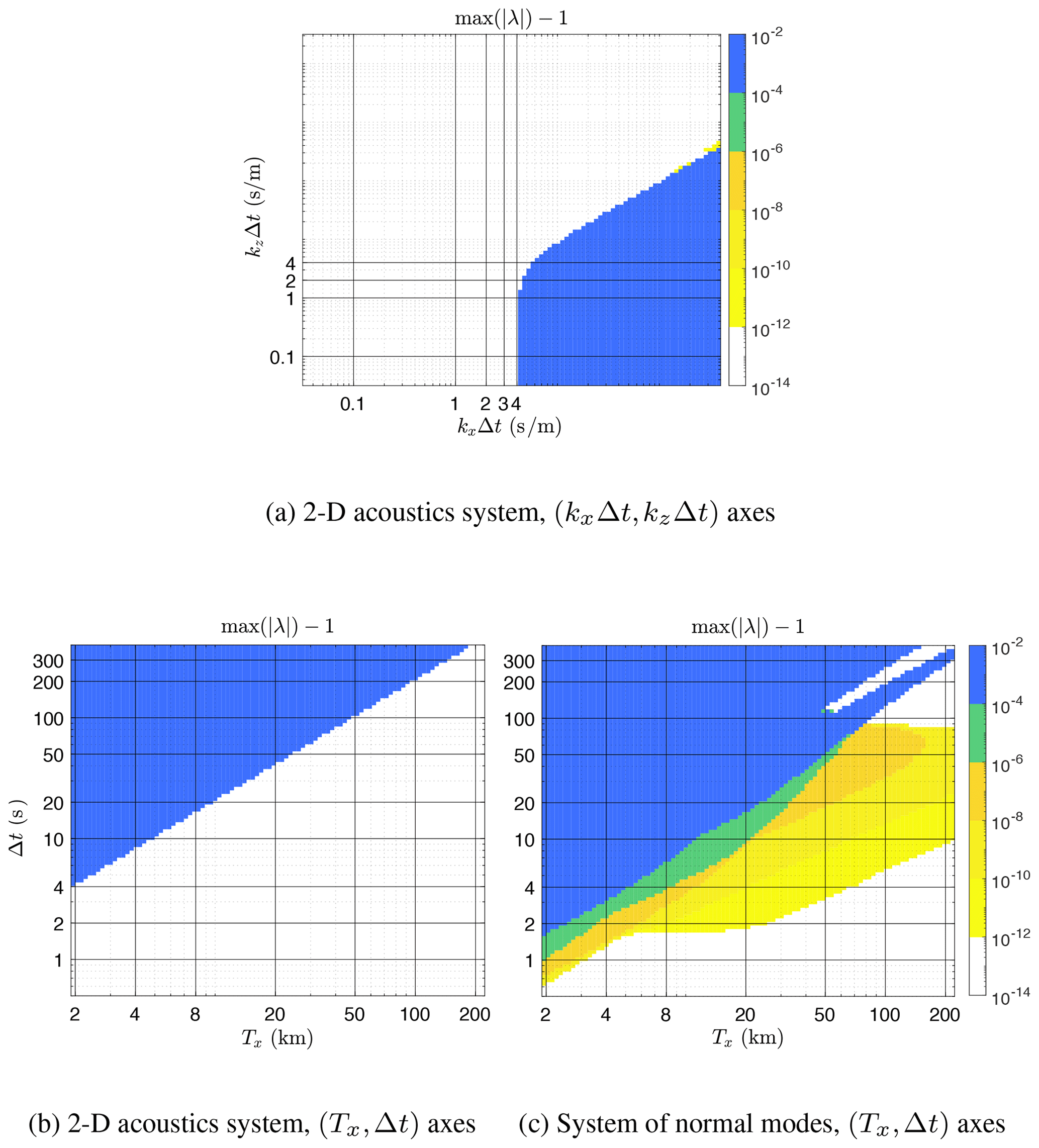
Figure 2Example of selectiveness of the new framework using the M1 method: the stability diagram (c) based on the system of normal modes which determines scheme M1 is unstable for practical applications, while time steps that are stable in the stability diagrams (a, b) based on the 2-D acoustic system look acceptable.
4.2 Schemes ARK2(2,3,2) (Giraldo et al., 2013) and IMEX-SSP2(2,3,2) (Rokhzadi et al., 2018)
In Rokhzadi et al. (2018), one of the ARK2(2,3,2) methods from Giraldo et al. (2013) is compared with a new scheme, IMEX-SSP2(2,3,2). The family of ARK2(2,3,2) schemes is characterized by parameter a32 in the explicit table (Giraldo et al., 2013). In Rokhzadi et al. (2018), the authors choose the method with , which we denote here as ARK2(2,3,2)(1). Rokhzadi et al. (2018) apply optimization to derive an ARK2 method with improved accuracy, stability, and strong stability preserving (SSP) properties relative to ARK2(2,3,2)(1) for a linear wave equation, the 2-D acoustics system, the compressible Boussinesq equations, and the van der Pol equation as in Durran and Blossey (2012), Weller et al. (2013), and Lock et al. (2014). We compare these two methods and method ARK2(2,3,2) with a32=0.85, which we denote ARK2(2,3,2)(2), using our system of normal modes (Eqs. 12–16). We conclude that ARK2(2,3,2)(2) and IMEX-SSP2(2,3,2) have very similar stability properties, as shown in Fig. 3b and c, but the stable (white) region for ARK2(2,3,2)(1) is significantly smaller, as shown in Fig. 3a.

Figure 3Schemes analyzed in Rokhzadi et al. (2018) and the ARK2(2,3,2)(2) scheme: (a) ARK2(2,3,2)(1), (b) ARK2(2,3,2)(2), and (c) IMEX-SSP2(2,3,2).
4.3 A set of low-storage, high-CFL IMEX schemes
We develop a set of methods we denote M2 using a second-order, explicit, low-storage, CFL-4 Runge–Kutta scheme from Kinnmark and Gray (1984a). Low-storage, high-CFL methods developed in Kinnmark and Gray (1984a) and Kinnmark and Gray (1984b) are used in HOMME, the nonhydrostatic atmospheric dynamical core of E3SM's atmosphere component. It is practical to extend existing explicit RK schemes to IMEX RK methods. We analyze the stability, dispersion, and dissipation properties of these M2 schemes using the system of normal modes (Eqs. 12–16).
4.3.1 Definitions
We start with the second-order explicit table (Eq. 30, top) from one of the methods in Kinnmark and Gray (1984a). For the implicit table (Eq. 30, bottom), we choose the same times for internal stages and make all but the last implicit stage backward Euler. Internal backward-Euler stages provide stability and do not affect the second-order accuracy conditions for IMEX given by Eqs. (25)–(26).
The M2 methods vary only in their last implicit stage. We require the last implicit stage to obey a stiffly accurate condition and have only non-negative entries in its table. The last stage is defined by the vector d, whose entries correspond to the last row of the implicit Butcher tableau, as shown in the table of Eq. (30), bottom. Moreover, here we consider only schemes with at most three nonzero entries in d to limit storage. In practice, using an IMEX method in a 3-D model with topography will require storing geopotential and vertical velocity terms for each internal stage that corresponds to , j1<ν. Therefore, we focus on methods that limit such storage space.
where
We consider the first- and second-order variants of the M2 methods listed in Table 1.
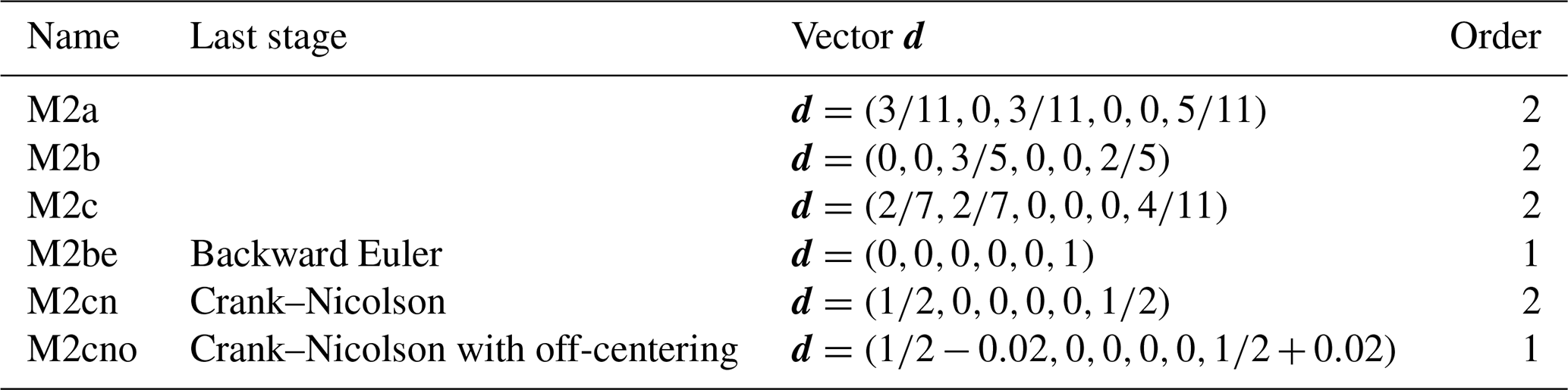
Variants M2a, M2b, and M2c, where M2c was introduced in Steyer et al. (2019), are second-order methods with good stability properties; their dispersive and dissipative characteristics are different, as shown below in Fig. 4. Variants M2be and M2cn are the two extremes of the M2 family. In M2be, the last stage is the backward-Euler method. Thus, it is first-order accurate, and we expect this scheme to be the most stable but also the most dissipative. We expect method M2cn, which has the Crank–Nicolson method for the last stage, to have no dissipation for hyperbolic problems like ours. We also analyze method M2cno, whose last stage is the Crank–Nicolson method with off-centering, since off-centering is a common approach to stabilize time-stepping schemes (Durran and Blossey, 2012; Staniforth et al., 2006).
4.3.2 Stability diagrams and dispersion and dissipation diagrams
Stability diagrams for the M2 schemes are shown in Figs. 4a–c and 5a–c, which follow the plotting procedures described in Sect. 4.1.1. We plot numerical frequencies of the space operator Q and the spacetime operator M to evaluate how the numerical time-stepping methods preserve the frequencies ω from the space discretization Q. Hyperbolicity of the system of Eqs. (12)–(16) implies exact time integration will conserve the frequencies. Inexact time integration will introduce errors, which we evaluate below. We also evaluate numerical damping since exact time integration has none. Note that we compare the properties of the spacetime operator with those of the space operator integrated exactly in time, but we do not compare solutions of the spacetime operator with analytical solutions of the system of Eqs. (12)–(16). This choice of comparison focuses on the numerical errors due solely to the time-stepping methods.
Dispersion and dissipation plots are shown below the stability diagrams, for the spacetime operator Q with eigenpairs (λj,qj), in Figs. 4d–f and 5d–f. In each figure, Δt=50 s and nlev=20. The top plots show numerical frequencies λj vs. vertical mode number. Red diamonds are numerical frequencies of the space operator for east- and west-propagating acoustic waves. Blue squares represent east- and west-propagating gravity waves for the space operator. Black diamonds are frequencies for west-propagating Rossby waves for the space operator. Red stars, blue plus signs, and black stars are for corresponding branches of the spacetime operator. Vertical mode number and wave characterization are obtained by uniquely matching eigenvector qj to its counterpart, eigenvector mk, of the space operator M, also computed using 20 vertical levels.
The bottom plots in Figs. 4d–f and 5d–f show the amplification factors of eigenvalues, , for the spacetime operator. The red stars, blue plus signs, and black stars are for acoustic, gravity, and Rossby waves, respectively. Each plot shows amplification factors near 1 for gravity and Rossby waves, with additional damping of the acoustic modes. We discuss these differences further in the next section.
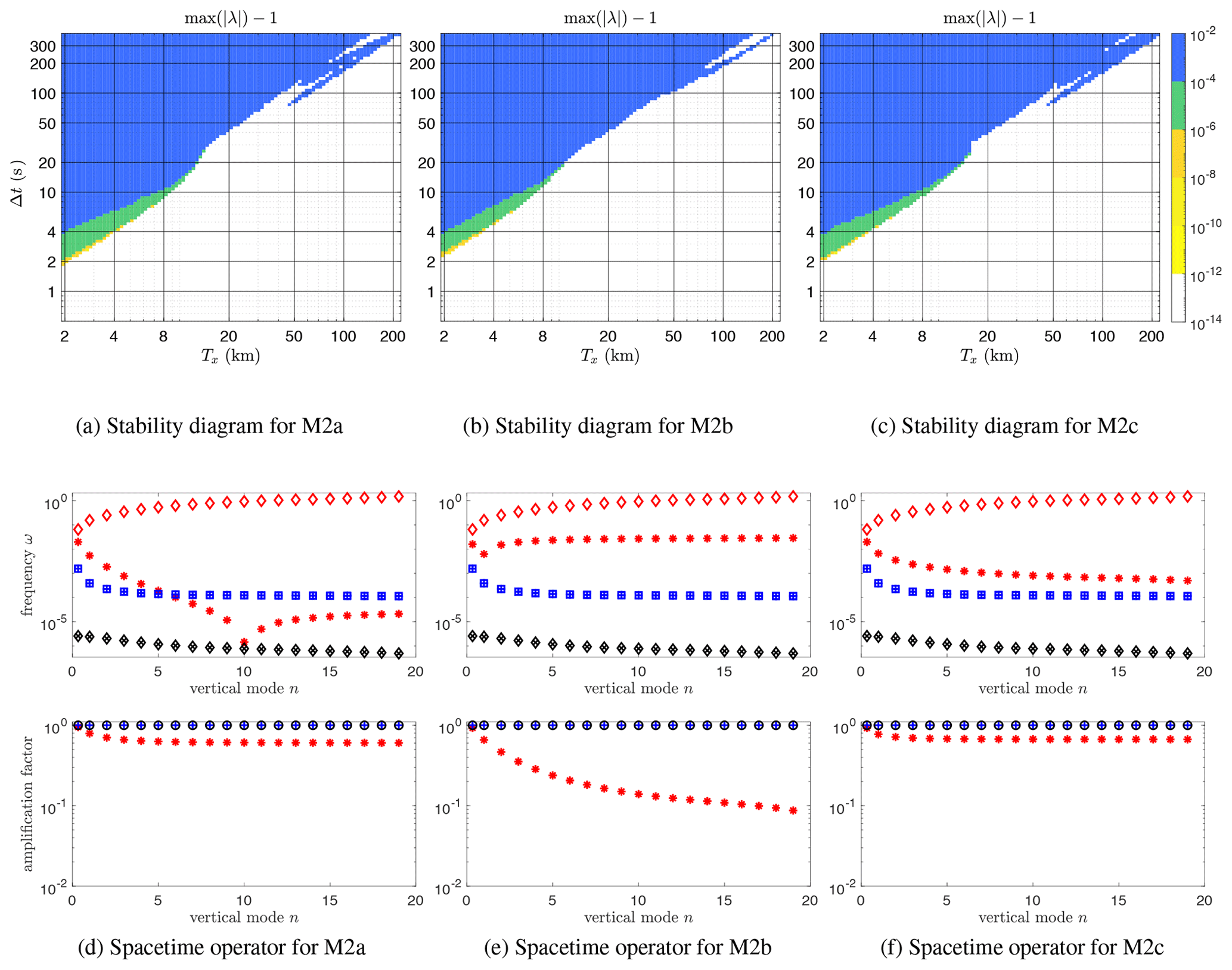
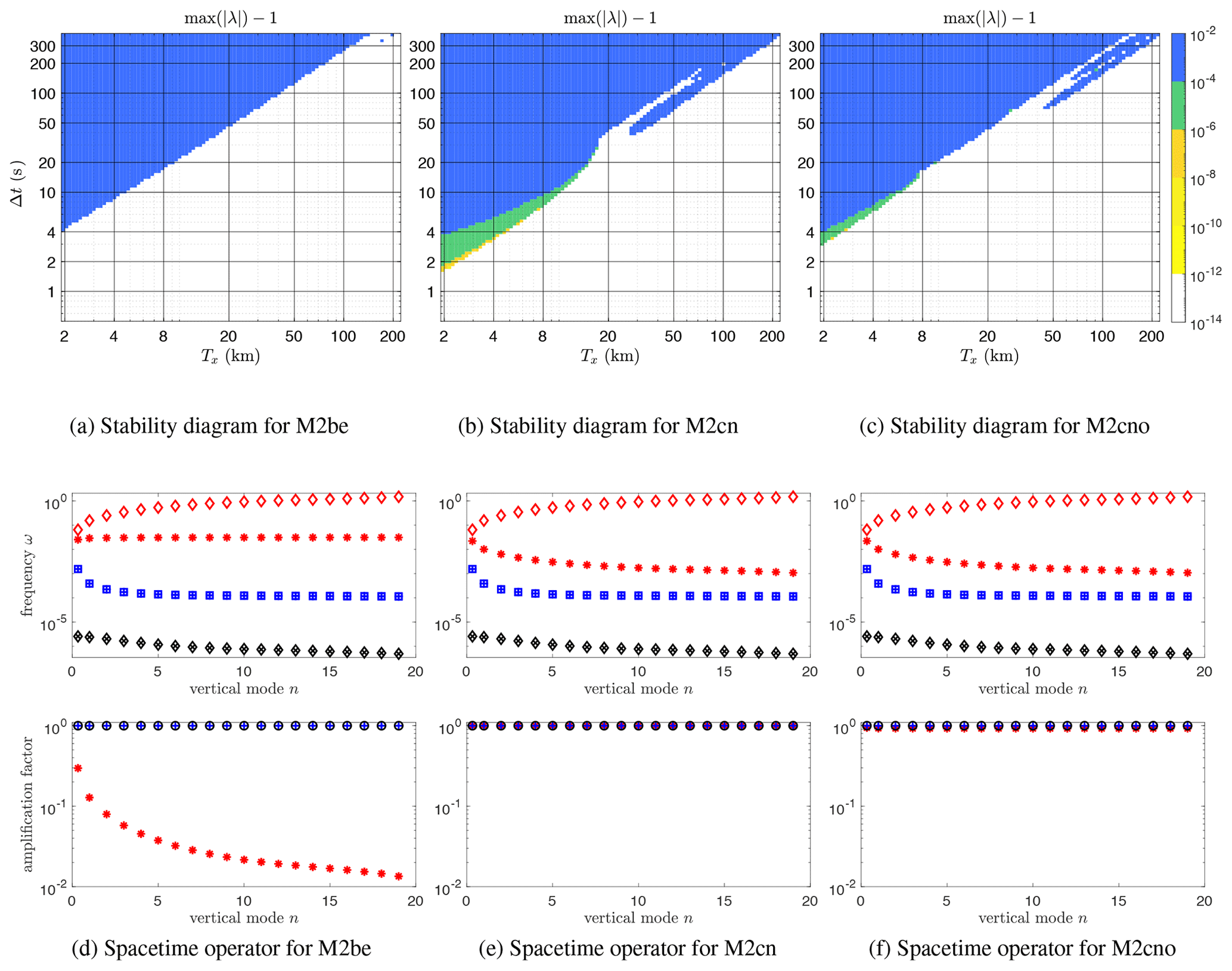
4.3.3 Analyzing the M2 schemes
Due to their different final stages, the M2 schemes have different stability properties and dispersive and dissipative characteristics. To evaluate stability, we focus on the regions having smallest spatial resolution and highest wavenumbers, since these are the regions where nonhydrostatic effects are most prominent. Evaluation of stability is easy: larger stable (white) regions imply larger stable Δt for those methods.
As expected, due to the presence of the last backward-Euler stage in the implicit table, the M2be scheme is the most stable. Recall that analytically for hyperbolic problems, the backward-Euler method is unconditionally stable and is very dissipative. For the M2be method, the largest stable Δt at Tx=2 km is approximately 4 s, which is at least twice as large as the largest stable Δt for the other schemes.
It is desirable to have an IMEX method with stability properties similar to those of an explicit method used for the non-stiff part of the system of Eq. (24). In other words, it is desirable to be able to integrate a nonhydrostatic system using an IMEX method with a time step as large as the time step used to integrate a hydrostatic system using an explicit Runge–Kutta method. Therefore, we compare the stability of the IMEX method M2be with the stability of the Runge–Kutta method consisting of the explicit table in M2be, a method we denote MExplicit, when it is applied to the non-stiff part of Eq. (24). The stability region of M2be in Fig. 5a is almost as big as the stability region of MExplicit (not shown here) up to a minor difference at approximate wavelength Tx=220 km. That is, the stability region of M2be is the biggest region we could possibly get from an IMEX scheme whose explicit table is part of the M2 set.
It is harder to rank schemes using dispersion and dissipation diagrams. All schemes preserve the dispersion and dissipation relations for gravity and Rossby waves to a high degree. But they perform very differently for acoustic waves. Method M2be has the largest dissipation for acoustic waves and is the only scheme that does not have regions of negative group velocity for acoustic waves. Method M2cn has opposite characteristics: it does not dampen acoustic waves, and the errors in the acoustic frequencies are much larger. M2cno, a first-order variation of M2cn, has dispersion errors that are very similar to M2cn while introducing low-degree dissipation into acoustic waves.
Since acoustic waves can be considered insignificant for atmospheric applications due to their low energy, one is tempted to discard numerical errors in the dispersion and dissipation of acoustic waves. However, there is an argument (Thuburn, 2012) that correct representation of even energetically weak waves in the atmosphere is crucial for accurate restoration of hydrostatic balance.
Among other second-order schemes (M2a, M2b, and M2c), it is hard to declare a clear winner. Due to its smaller largest stable Δt at Tx=2 km and large dispersion errors, M2a may be less competitive. Compared with M2c, M2b has slightly larger maximum stable Δt at Tx=2 km, and its errors in dispersion for acoustic waves are smaller, but its dissipation is larger. Indeed, its larger dissipation is probably what causes its better stability compared with M2c. However, depending on the evaluation criteria, M2c can be viewed as a better scheme than M2b. For example, it has less dissipation and its dispersion is very similar to that of the Crank–Nicolson method, which is widely used for hyperbolic problems.
4.3.4 Role of the implicit table
We chose to limit our search for a suitable M2 method by varying only the vector d in the implicit table. Since the second-order accuracy conditions for the M2 family depend only on the last implicit stage, we make all other implicit stages (stages 2–5) use the backward-Euler method to presumably maximize stability. One could also try to use Crank–Nicolson or off-centered Crank–Nicolson methods for implicit stages 2–5.
To understand how the implicit stages influence dissipation of acoustic waves, we consider the expression for the final solution of Eq. (24) using Lock et al. (2014), Eq. (15), and the definition of the M2 family in Eq. (30):
Scheme M2cn, given by its final implicit stage , does not have dissipation. For M2cn, the solution yn+1 is directly influenced by intermediate implicit stages 2–5 only by the non-stiff term. Also, its final implicit stage is represented by the Crank–Nicolson method, known to be non-dissipative for hyperbolic problems. We conclude that both of these facts contribute to the lack of dissipation in M2cn. Scheme M2be has final implicit stage , which gives the backward-Euler method. Similarly to the backward-Euler method for hyperbolic problems, M2be is very dissipative.
We suggest that the dispersion and dissipation of acoustics waves can be tuned by working only with the implicit table of any method.
4.4 Stability properties with respect to vertical resolution
For an explicit time-stepping method, the most restrictive CFL condition is usually that associated with the vertically propagating acoustic waves and the stable time step decreases linearly with . Ideally, with an implicit treatment of vertical acoustic waves, an IMEX method should remain stable as nlev is increased, and the stability should be controlled only by the CFL condition associated with the horizontal resolution.
To analyze this aspect of various IMEX methods, we fix kx to the highest frequency resolvable by a model with 3 km grid spacing and vary the number of vertical levels from nlev=20 to nlev=100. We plot the method's stability as a function of nlev using a logarithmic scale (up to rounding to the nearest integer) and 50 sample points. The stability diagrams are made very similarly to the ones in Fig. 4; the only difference is the horizontal axis, which now is nlev. We vary Δt from 1 to 10 s with logarithmic spacing and 100 samples. Note that the horizontal axis is not defined by a vertical wavenumber, kz, because for any fixed resolution Δz the model supports waves with many vertical wavenumbers.
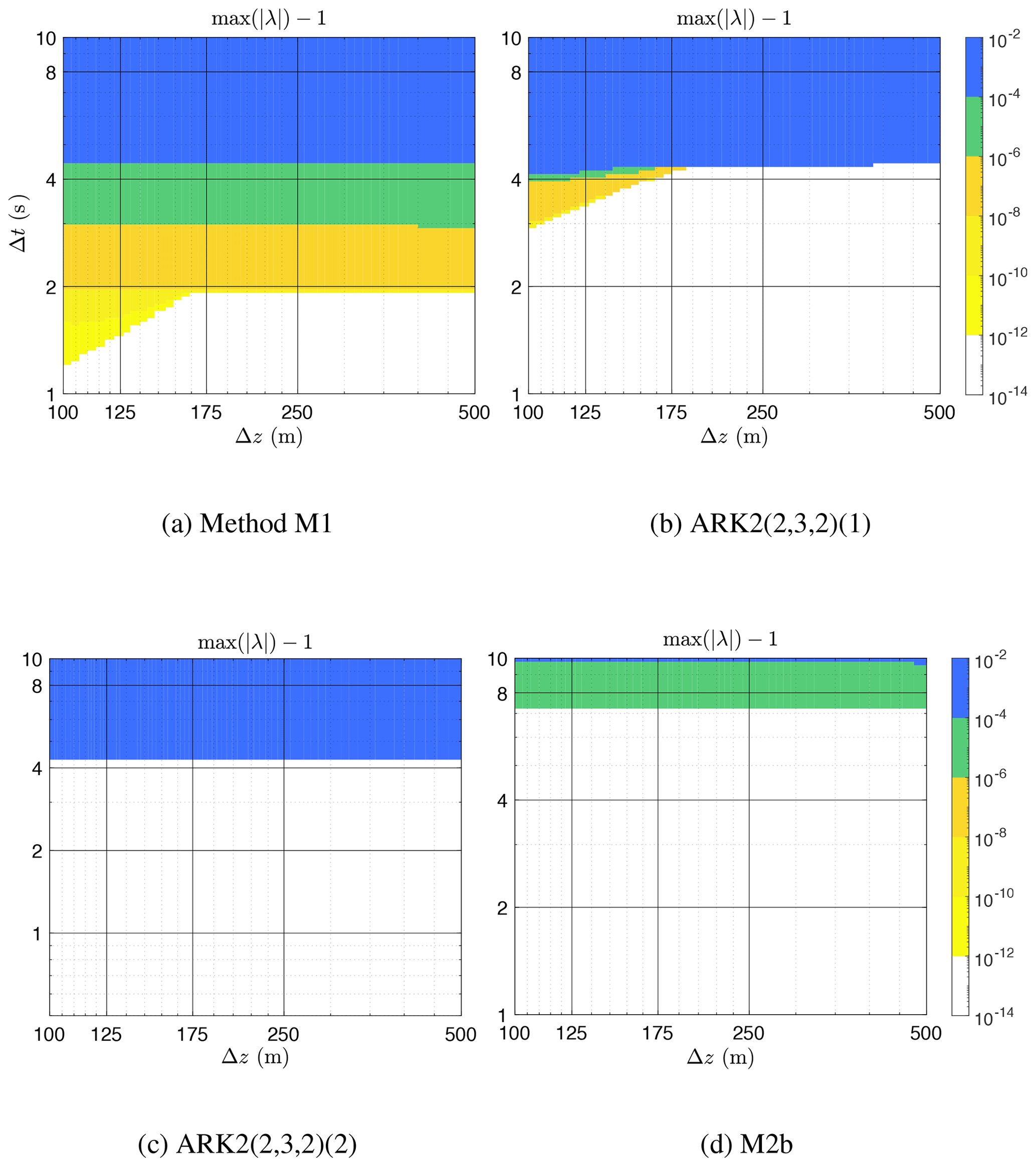
Figure 6 contains stability diagrams for schemes M1, ARK2(2,3,2)(1), ARK2(2,3,2)(2), and M2b. For schemes M1 and ARK2(2,3,2)(1), the stability is independent of Δz, as desired, only for up to approximately nlev=57 (Δz≃175 m). In Fig. 6a–b, the stable region for the approximate interval ( m) is under a straight line for some Δt=Δt0. For finer Δz, the stable regions lie below a line with a constant slope for both schemes.
In contrast, for methods ARK2(2,3,2)(2) and M2b, stability is always controlled by the horizontal resolution: in Fig. 6c, the stable region is below the horizontal line Δt0≃7.2 s. To further support this conclusion, we also computed eigenvalues of the spacetime operator for method M2b, Δt=7 s, and a few large values of nlev, up to 600. The spacetime operator for all large nlev was stable.
We do not present stability diagrams for Δz studies for other methods from this paper because they are identical to Fig. 6c up to the value of Δt0. That is, the stability of methods IMEX-SSP2(2,3,2) and M2 methods is controlled by the horizontal wavelengths.
We developed a new framework to evaluate IMEX RK methods for atmospheric modeling. The framework uses a system of normal modes and is proven to be simple but more selective than the 2-D acoustics system used in the literature. For example, the M1 method from Sect. 4.1 appears to be stable for a large set of time steps and resolutions when using the 2-D acoustics system. If the method is evaluated with the system of normal modes, it is unstable for the same set of time steps and resolutions.
The new framework gives us insight to develop a set of second-order, low-storage, high-CFL IMEX RK methods to use in atmospheric dynamical cores. Furthermore, we use the spacetime operator built with the system of normal modes to investigate dispersion and dissipation of IMEX RK schemes for three types of waves: gravity, Rossby, and acoustic.
One extension of this work would be to investigate selectiveness of the framework based not on the system of normal modes (Eqs. 12–16) but on a system of compressible Boussinesq equations as in Durran and Blossey (2012).
The current version of scripts is available from the project website (https://github.com/E3SM-Project/sta-imex, last access: 19 December 2020) under the BSD three-clause license. The exact version of the model used to produce the results used in this paper is archived on Zenodo (Guba and Steyer, 2020, https://doi.org/10.5281/zenodo.3785712). Scripts for the work presented here were written in MATLAB and executed in MATLAB R2018b. Descriptions of the scripts are provided in file README, which is archived with the scripts in Guba and Steyer (2020). To reproduce the dispersion and dissipation plots, one needs to download the implementation of the Munkres algorithm for MATLAB separately at Cao (2020).
For this submission, we created the script paper_figures.m, also archived on Zenodo (Guba and Steyer, 2020), which sets parameters and launches the MATLAB scripts to produce all paper figures in the order they appear.
The script contains comments to easily identify the figures.
Sta-imex version 1.0: Copyright 2020 National Technology & Engineering Solutions of Sandia, LLC (NTESS). Under the terms of contract DE-NA0003525 with NTESS, the US Government retains certain rights in this software. For the full copyright statement, see Guba and Steyer (2020).
OG wrote the manuscript with contributions from PAB and AMB. OG, MAT, and AMB contributed to the design of the framework. OG and AS developed software for the framework.
The authors declare that they have no conflict of interest.
Sandia National Laboratories is a multimission laboratory managed and operated by National Technology and Engineering Solutions of Sandia, LLC, a wholly owned subsidiary of Honeywell International Inc., for the US Department of Energy's National Nuclear Security Administration under contract DE-NA0003525. This paper describes objective technical results and analysis. Any subjective views or opinions that might be expressed in the paper do not necessarily represent the views of the US Department of Energy or the United States Government.
SAND2020-5447 J
The authors thank an anonymous reviewer and Emil Constantinescu for their valuable comments and suggestions.
This research was supported as part of the Energy Exascale Earth System Model (E3SM) project, funded by the US Department of Energy (DOE), Office of Science, Office of Biological and Environmental Research (BER), and by the DOE Office of Science, Advanced Scientific Computing Research (ASCR) Program under the Scientific Discovery through Advanced Computing (SciDAC 4) ASCR/BER Partnership Program.
This research has been supported by the US DOE, Office of Science.
This paper was edited by Simon Unterstrasser and reviewed by Emil Constantinescu and one anonymous referee.
Cao, Y.: Munkres Assignment Algorithm, available at: https://www.mathworks.com/matlabcentral/fileexchange/20328-munkres-assignment-algorithm, last access: 22 March 2020. a, b
Dennis, J., Edwards, J., Evans, K., Guba, O., Lauritzen, P., Mirin, A., St-Cyr, A., Taylor, M. A., and Worley, P. H.: CAM-SE: A scalable spectral element dynamical core for the Community Atmosphere Model, Int. J. High Perf. Comput. Appl., 26, 74–89, 2012. a
Durran, D. and Blossey, P.: Implicit-Explicit Multistep Methods for Fast-Wave-Slow-Wave Problems, Mon. Weather Rev., 140, 1307–1325, https://doi.org/10.1175/MWR-D-11-00088.1, 2012. a, b, c, d, e
Giraldo, F., Kelly, J., and Constantinescu, E.: Implicit-Explicit Formulations of a Three-Dimensional Nonhydrostatic Unified Model of the Atmosphere (NUMA), SIAM J. Sci. Comput., 35, B1162–B1194, https://doi.org/10.1137/120876034, 2013. a, b, c, d
Guba, O. and Steyer, A.: E3SM-Project/sta-imex: v1.0.5 (Version v1.0.5), Zenodo, https://doi.org/10.5281/zenodo.3785712 (last access: 9 October 2020), 2020. a, b, c, d
Kinnmark, I. and Gray, W.: One step integration methods with maximum stability regions, Math. Comput. Simulat., XXVI, 84–92, https://doi.org/10.1016/0378-4754(84)90039-9, 1984a. a, b, c
Kinnmark, I. and Gray, W.: One step integration methods with third-fourth order accuracy with large hyperbolic stability limits, Math. Comput. Simulat., XXVI, 181–188, https://doi.org/10.1016/0378-4754(84)90056-9, 1984b. a, b
Laprise, R.: The Euler equations of motion with hydrostatic pressure as an independent variable, Mon. Weather Rev., 120, 197–207, 1992. a
Lin, S.-J.: A Vertically Lagrangian Finite-Volume Dynamical Core for Global Models, Mon. Weather Rev., 132, 2293–2397, 2004. a
Lock, S.-J., Wood, N., and Weller, H.: Numerical analyses of Runge-Kutta implicit-explicit schemes for horizontally explicit, vertically implicit solutions of atmospheric models, Q. J. Roy. Meteor. Soc., 140, 1654–1669, https://doi.org/10.1002/qj.2246, 2014. a, b, c, d, e, f, g, h, i, j, k
Munkres, J.: Algorithms for the Assignment and Transportation Problems, J. Soc. Ind. Appl. Math., 5, 32–38, 1957. a
Rasch, P. J., Xie, S., Ma, P.-L., Lin, W., Wang, H., Tang, Q., Burrows, S. M., Caldwell, P., Zhang, K., Easter, R. C., Cameron-Smith, P., Singh, B., Wan, H., Golaz, J.-C., Harrop, B. E., Roesler, E., Bacmeister, J., Larson, V. E., Evans, K. J., Qian, Y., Taylor, M., Leung, L., Zhang, Y., Brent, L., Branstetter, M., Hannay, C., Mahajan, S., Mametjanov, A., Neale, R., Richter, J. H., Yoon, J.-H., Zender, C. S., Bader, D., Flanner, M., Foucar, J. G., Jacob, R., N.Keen, Klein, S. A., Liu, X., Salinger, A. G., and Shrivastava, M.: An Overview of the Atmospheric Component of the Energy Exascale Earth System Model, J. Adv. Model. Earth Syst., 11, 2377–2411, https://doi.org/10.1029/2019MS001629, 2019. a
Rokhzadi, A., Mohammadian, A., and Charron, M.: An Optimally Stable and Accurate Second-Order SSP Runge-Kutta IMEX Scheme for Atmospheric Applications, J. Adv. Model. Earth Syst., 10, 18–42, https://doi.org/10.1002/2017MS001065, 2018. a, b, c, d, e, f, g, h, i
Staniforth, A., White, A., Wood, N., Thuburn, J., Zerroukat, M., Cordero, E., Davies, T., and Diamantakis, M.: UNIFIED MODEL DOCUMENTATION PAPER No 15, Tech. rep., United Kingdom Met Office, Exeter, Devon, available at: http://research.metoffice.gov.uk/research/nwp/publications/papers/unified_model/umdp15_v6.3.pdf (last access: 26 February 2017), 2006. a
Steyer, A., Vogl, C. J., Taylor, M., and Guba, O.: Efficient IMEX Runge-Kutta methods for nonhydrostatic dynamics, arXiv e-prints, arXiv:1906.07219, 2019. a, b, c, d
Taylor, M. A., Guba, O., Steyer, A., Ullrich, P. A., Hall, D. M., and Eldrid, C.: An Energy Consistent Discretization of the Nonhydrostatic Equations in Primitive Variables, J. Adv. Model. Earth Syst., 12, e2019MS001783, https://doi.org/10.1029/2019MS001783, 2020. a, b
Thuburn, J.: Some Basic Dynamics Relevant to the Design of Atmospheric Model Dynamical Cores, in: Numerical Techniques for Global Atmospheric Models, edited by: Lauritzen, P. H., Jablonowski, C., Taylor, M. A., and Nair, R. D., Springer, 2012. a
Thuburn, J. and Woollings, T. J.: Vertical Discretizations for Compressible Euler Equation Atmospheric Models Giving Optimal Representation of Normal Modes, J. Comput. Phys., 203, 386–404, 2005. a, b
Thuburn, J., Wood, N., and Staniforth, A.: Normal modes of deep atmospheres. I: Spherical geometry, Q. J. Roy. Meteor. Soc., 128, 1771–1792, https://doi.org/10.1256/003590002320603403, 2002a. a, b
Thuburn, J., Wood, N., and Staniforth, A.: Normal modes of deep atmospheres. II: f–F-plane geometry, Q. J. Roy. Meteor. Soc., 128, 1793–1806, https://doi.org/10.1256/003590002320603412, 2002b. a, b, c
Weller, H., Lock, S.-J., and Wood, N.: Runge-Kutta IMEX schemes for the Horizontally Explicit/Vertically Implicit (HEVI) solution of wave equations, J. Comput. Phys., 252, 365–381, https://doi.org/10.1016/j.jcp.2013.06.025, 2013. a, b, c, d, e, f