On the tuning of atmospheric inverse methods: comparisons with the European Tracer Experiment (ETEX) and Chernobyl datasets using the atmospheric transport model FLEXPART

Estimation of the temporal profile of an atmospheric release, also called the source term, is an important problem in environmental sciences. The problem can be formalized as a linear inverse problem wherein the unknown source term is optimized to minimize the difference between the measurements and the corresponding model predictions. The problem is typically ill-posed due to low sensor coverage of a release and due to uncertainties, e.g., in measurements or atmospheric transport modeling; hence, all state-of-the-art methods are based on some form of regularization of the problem using additional information. We consider two kinds of additional information: the prior source term, also known as the first guess, and regularization parameters for the shape of the source term. While the first guess is based on information independent of the measurements, such as the physics of the potential release or previous estimations, the regularization parameters are often selected by the designers of the optimization procedure. In this paper, we provide a sensitivity study of two inverse methodologies on the choice of the prior source term and regularization parameters of the methods. The sensitivity is studied in two cases: data from the European Tracer Experiment (ETEX) using FLEXPART v8.1 and the caesium-134 and caesium-137 dataset from the Chernobyl accident using FLEXPART v10.3.

1 Introduction

The source term describes the spatiotemporal distribution of an atmospheric release, and it is of great interest in the case of an accidental atmospheric release. The aim of inverse modeling is to reconstruct the source term by maximization of agreement between the ambient measurements and prediction of an atmospheric transport model in a so-called top-down approach (Nisbet and Weiss, 2010). Since information provided by the measurements is often insufficient in both spatial and temporal domains (Mekhaimr and Wahab, 2019), additional information and regularization of the problem are crucial for a reasonable estimation of the source term (Seibert et al., 2011). Otherwise, the top-down determination of the source term can produce artifacts, often resulting in some completely implausible values of the source term. One common regularization is the knowledge of the prior source term, also known as the first guess, considered within the optimization procedure (Eckhardt et al., 2008; Liu et al., 2017; Chai et al., 2018). However, this knowledge could dominate the resulting estimate and even outweigh the information present in the measured data. The aim of this study is to discuss drawbacks that may arise in setting the prior source term and to study the sensitivity of inversion methods to the choice of the prior source term. We utilize the ETEX (European Tracer Experiment) and Chernobyl datasets for demonstration.

We assume that the measurements can be explained by a linear model using the concept of the source–receptor sensitivity (SRS) matrix calculated from an atmospheric transport model (e.g., Seibert and Frank, 2004). The problem can be approached by a constrained optimization with selected penalization term on the source term (Davoine and Bocquet, 2007; Ray et al., 2015; Henne et al., 2016) and further with an additional smoothness constraint (Eckhardt et al., 2008) used for both spatial (Stohl et al., 2011) and temporal (Seibert et al., 2011; Stohl et al., 2012; Evangeliou et al., 2017) profile smoothing. The optimization terms are typically weighted by covariance matrices whose forms and estimation have been studied in the literature. Diagonal covariance matrices have been considered by Michalak et al. (2005) and its entries estimated using the maximum likelihood method. Since the estimation of full covariance matrices tends to diverge (Berchet et al., 2013), approaches using a fixed common autocorrelation timescale parameter for non-diagonal entries has been introduced (Ganesan et al., 2014; Henne et al., 2016) for atmospheric gas inversion. Uncertainties can be also reduced with the use of ensemble techniques (see, e.g., Evensen, 2018; Carrassi et al., 2018, and references therein) when such an ensemble is available in the form of several meteorological input datasets and/or variations in atmospheric model parameters. Even with only one SRS matrix, the problem can be formulated as a probabilistic hierarchical model with unknown parameters estimated together with the source term with constraints such as positivity, sparsity, and smoothness (Tichý et al., 2016). The drawback of these methods is the necessity of selection and tuning of various model parameters, with the selection of the prior source term and its uncertainty being the most important.

There are various assumptions on the level of knowledge of the prior source term used in the inversion procedure. Assumption of the zero prior source term (Bocquet, 2007; Tichý et al., 2016) is common in the literature with a preference for a zero solution on elements whereby no sufficient information from data is available. This assumption is typically formalized as the Tikhonov (Golub et al., 1999) or LASSO (Tibshirani, 1996) regularizations or their variants. Soft assumptions in the form of the scale of the prior source term (Davoine and Bocquet, 2007), bounds on emissions (Miller et al., 2014), or even knowledge of total released amount as discussed, e.g., in Bocquet (2005) can be considered. One can also assume the ratios between species in multispecies source term scenarios (Saunier et al., 2013; Tichý et al., 2018). However, the majority of inversion methods explicitly assume knowledge of the prior source term (Connor et al., 2008; Eckhardt et al., 2008; Liu et al., 2017). This is more or less justified by appropriate construction of the prior source term based, for example, on a detailed analysis of an inventory and accident (Stohl et al., 2012), on previous estimates when available (Evangeliou et al., 2017), or on measured or observed data (Stohl et al., 2011). While in well-documented cases this approach could be well-justified, in cases with very limited available information or even complete absence of information on the source term, such as the iodine occurrence over Europe in 2017 (Masson et al., 2018) and the unexpected detection of ruthenium in Europe in 2017 (Bossew et al., 2019; Saunier et al., 2019), the use of strong prior source term assumptions could lead to prior-dominated results with limited validity. Although the choice of the prior source term is crucial, few studies have discussed the choice of the prior source term in detail and provided sensitivity studies on this selection as in Seibert et al. (2011) for the temporal profile of sulfur dioxide emissions and in Stohl et al. (2009) for the spatial distribution of greenhouse gas emissions.

The aim of this paper is to explore the sensitivity of linear inversion methods to the prior source term selection coupled with tuning of the covariance matrix representing modeling error. We considered the optimization method proposed by Eckhardt et al. (2008), as well as its probabilistic counterpart formulated as the hierarchical Bayesian model, extended here by a nonzero prior source term with variational Bayes' inference (Tichý et al., 2016) and with Monte Carlo inference using a Gibbs sampler (Ulrych and Šmídl, 2017). Two real cases will be examined: the ETEX (Nodop et al., 1998) and Chernobyl (Evangeliou et al., 2016) datasets. ETEX provides ideal data for a prior source term sensitivity study since the emission profile is exactly known. We propose various modifications of the known prior source term and study their influence on the results of the selected inversion methods. The Chernobyl dataset, on the other hand, provides a very demanding case in which only consensus on the release is available and the source term is more speculative.

2 Inverse modeling using the prior source term

We are concerned with linear models of atmospheric dispersion using an SRS matrix (Seibert, 2001; Wotawa et al., 2003; Seibert and Frank, 2004), which has been used in inverse modeling (Evangeliou et al., 2017; Liu et al., 2017). Here, the atmospheric transport model calculates the linear relationship between potential sources and atmospheric concentrations. The source–receptor sensitivity is calculated as $m_{ij}=c_i/x_j$, where x_j is the assumed release from the release site at time j and c_i is the calculated concentration at a receptor c_i at the respective time period. The measurement y_i at a given time and location can be explained as a sum of contributions from all elements of the source term weighted by m_ij. In matrix notation,

$$\begin{array}{}\text{(1)}& \mathit{y}=\mathbf{M}\mathit{x}+\mathit{e},\end{array}$$

where y∈ℜ^p is a vector aggregating measurements from all locations and times (in arbitrary order), and x∈ℜⁿ is a vector of all possible releases from a given time period and all possible source–receptor sensitivities form the SRS matrix $\mathbf{M}\in {\mathrm{\Re }}^{p\times n}$. The residual model, e∈ℜ^p, is a sum of model and measurement errors. While the model looks trivial, its use in practical applications poses significant challenges. The key reason is that all elements of the model are subject to uncertainty (Winiarek et al., 2012; Liu et al., 2017) and the problem is ill-posed.

In the rest of this section, we will discuss an influence of the modeling error and show how existing methods approach compensation of such error. We will analyze in detail two methods for the source term estimation: (i) the optimization model proposed by Eckhardt et al. (2008) with a prior source term already considered and (ii) a Bayesian model (Tichý et al., 2016) extended here by prior source term information and solved using both the variational Bayes' method and the Gibbs sampling method.

2.1 Influence of atmospheric model error

It is generally assumed that the SRS matrix M is correct and the true source term minimizes error of y=Mx. However, M is prone to errors due to a number of approximations in the formulation of the atmospheric transport model and use of uncertain weather analysis data as input to the atmospheric transport model. Therefore, one should rather consider a hypothetical model,

$$\begin{array}{}\text{(2)}& \mathit{y}=\left(\mathbf{M}+{\mathrm{\Delta }}_{\mathbf{M}}\right)\mathit{x},\end{array}$$

where M is the available estimate of the sensitivity matrix from a numerical model, and the term Δ_M is the deviation of the estimate from the true generating matrix, ${\mathbf{M}}_{\text{true}}=(\mathbf{M}+{\mathrm{\Delta }}_{\mathbf{M}})$. Exact estimation of Δ_M is not possible due to a lack of data; however, many existing regularization techniques can be interpreted as various simplified parameterizations of Δ_M.

The L2 norm¹ of the residuum between measurement and reconstruction for Eq. (3) would become

$$\begin{array}{ll}{\displaystyle }\left|\right|\mathit{y}-\mathbf{M}\mathit{x}-{\mathrm{\Delta }}_{\mathbf{M}}\mathit{x}|{|}_{\mathrm{2}}^{\mathrm{2}}& {\displaystyle }=\left|\right|\mathit{y}-\mathbf{M}\mathit{x}|{|}_{\mathrm{2}}^{\mathrm{2}}-\mathrm{2}{\mathit{y}}^T{\mathrm{\Delta }}_{\mathbf{M}}\mathit{x}+{\mathit{x}}^T\mathrm{\Phi }\mathit{x}\\ \text{(3)}& {\displaystyle }\mathrm{\Phi }& {\displaystyle }={\mathbf{M}}^T{\mathrm{\Delta }}_{\mathbf{M}}+{\mathrm{\Delta }}_{\mathbf{M}}^T\mathbf{M}+{\mathrm{\Delta }}_{\mathbf{M}}^T{\mathrm{\Delta }}_{\mathbf{M}}.\end{array}$$

The ideal optimization problem (right-hand side of Eq. 3) can be decomposed into the norm of residues of the estimated model $\left|\right|\mathit{y}-\mathbf{M}\mathit{x}|{|}_{\mathrm{2}}^{\mathrm{2}}$, with both linear (i.e., −2y^TΔ_Mx) and quadratic terms in x (i.e., x^TΦx). Both of the additional terms contribute to incorrect estimation of x when Δ_M is significant.

An common attempt to minimize the influence of the linear term is to define the prior source term x^a and subtract Mx^a from both sides of Eq. (2). This yields a new decomposition derived in Appendix A (with substitutions $\stackrel{\mathrm{‾}}{\mathit{x}}=\mathit{x}-{\mathit{x}}^a$ and $\stackrel{\mathrm{‾}}{\mathit{y}}=\mathit{y}-\mathbf{M}{\mathit{x}}^a$) as

$$\begin{array}{}\text{(4)}& \begin{array}{rl}& \left|\right|\mathit{y}-\mathbf{M}\mathit{x}-{\mathrm{\Delta }}_{\mathbf{M}}\mathit{x}|{|}_{\mathrm{2}}^{\mathrm{2}}=||\stackrel{\mathrm{‾}}{\mathit{y}}-\mathbf{M}\stackrel{\mathrm{‾}}{\mathit{x}}|{|}_{\mathrm{2}}^{\mathrm{2}}-\mathrm{2}\left({\stackrel{\mathrm{‾}}{\mathit{y}}}^T{\mathrm{\Delta }}_{\mathbf{M}}\right.\\ & \left.-{\left({\mathrm{\Delta }}_{\mathbf{M}}{\mathit{x}}^a\right)}^T\mathbf{M}-{\left({\mathrm{\Delta }}_{\mathbf{M}}{\mathit{x}}^a\right)}^T{\mathrm{\Delta }}_{\mathbf{M}}\right)\stackrel{\mathrm{‾}}{\mathit{x}}+{\stackrel{\mathrm{‾}}{\mathit{x}}}^T\mathrm{\Phi }\stackrel{\mathrm{‾}}{\mathit{x}},\end{array}\end{array}$$

where Φ is the same term as in Eq. (3).

In the ideal situation, we would like to optimize the left-hand side of Eqs. (3) and (4). However, due to unavailability of Δ_M the linear term is typically ignored (assumed to be negligible) and the quadratic term is approximated using a parametric form of Φ≈Ξ. The optimization criterion is then

$$\begin{array}{}\text{(5)}& J=\left|\right|\stackrel{\mathrm{‾}}{\mathit{y}}-\mathbf{M}\stackrel{\mathrm{‾}}{\mathit{x}}|{|}_{\mathrm{2}}^{\mathrm{2}}+{\stackrel{\mathrm{‾}}{\mathit{x}}}^T\mathrm{\Xi }\stackrel{\mathrm{‾}}{\mathit{x}}.\end{array}$$

The estimation error caused by approximation (5) can be influenced by two choices of the user: (i) first guess x^a and (ii) regularization matrix Ξ. The purpose of choosing x^a is minimization of the linear term in Eq. (4). The choice of the parametric form of Ξ corresponds to choosing a model of the SRS matrix error Δ_M, since Ξ is an approximation of Φ, which is determined by Δ_M.

In the following sections, we will discuss methods that estimate Ξ from the data using parameterization of Ξ by tri-diagonal matrices with a limited number of parameters. Specifically, we will investigate if the choice of x^a has an impact on better estimation of Ξ.

2.2 Optimization approach

In Eckhardt et al. (2008), the source term inversion problem is formulated as in Eq. (5) with choices

$$\begin{array}{}\text{(6)}& \mathrm{\Xi }=\mathbf{B}+\mathit{ϵ}{\mathbf{D}}^T\mathbf{D},\end{array}$$

where matrix B is the selected or estimated precision matrix, the matrix D a discrete representation of the second derivative with diagonal elements equal to −2 and equal to 1 on the first sub-diagonals, and the scalar ϵ is the parameter weighting the smoothness of the solution x.

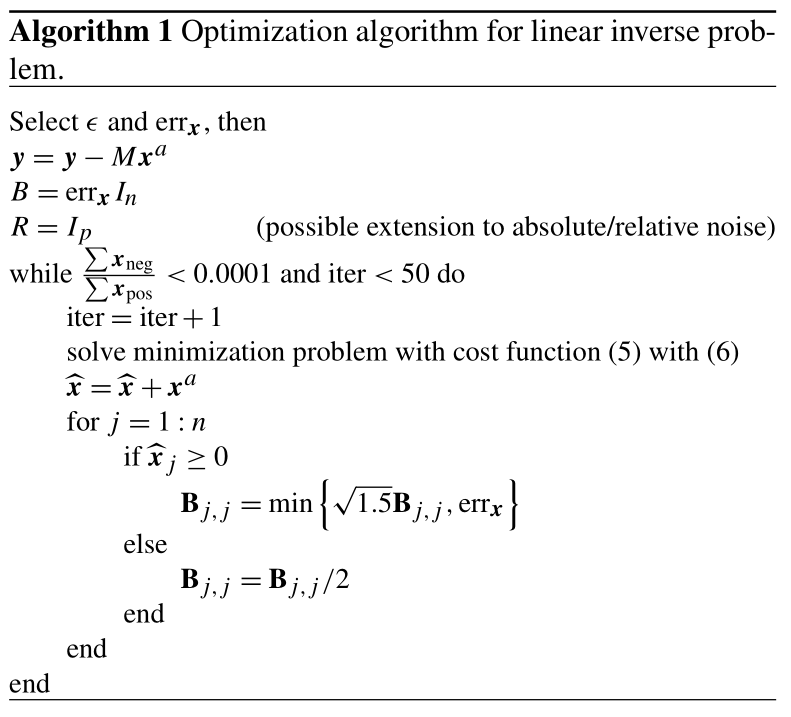
Minimization of Eq. (5) does not guarantee the non-negativity of the estimated source term x. To solve this issue, an iterative procedure is adopted (Eckhardt et al., 2008) whereby minimization of Eq. (5) is done repetitively with reduced diagonal elements of B related to the negative parts of the solution, thus tightening the solution to the prior source term, which is assumed to be non-negative. The diagonal elements of B related to the positive parts of the solution can, on the other hand, be enlarged up to a selected constant. This can be iterated until the absolute value of the sum of negative source term elements is lower than 0.01 % of the sum of positive source term elements. Formally, B_j,j in the ith iteration is calculated as

$$\begin{array}{}\text{(7)}& {\mathbf{B}}_{j,j}^{\left(i\right)}=\left\{\begin{array}{ll}\mathrm{0.5}{\mathbf{B}}_{j,j}^{(i-\mathrm{1})}& \text{for }{\mathit{x}}_j^{(i-\mathrm{1})}<\mathrm{0},\\ min\mathit{\{}\sqrt{\mathrm{1.5}}{\mathbf{B}}_{j,j}^{(i-\mathrm{1})},{\text{err}}_{\mathit{x}}\mathit{\}}& \text{for }{\mathit{x}}_j^{(i-\mathrm{1})}\ge \mathrm{0}.\end{array}\right.\end{array}$$

We observed very low sensitivity to the choice of the recommended values of 0.5 and $\sqrt{\mathrm{1.5}}$ in Eq. (7). In most cases, varying these values does not lead to any serious differences in the resulting estimate. However, the selection of parameters x^a, err_x, and ϵ is crucial and will be discussed in Sect. 2.4.

The method is summarized as Algorithm 1 and will be denoted as the optimization method in this study. The maximum number of iterations is set to 50, which was enough for convergence in all our experiments. To solve the minimization problem (5), we use the CVX toolbox (Grant and Boyd, 2008, 2018) for MATLAB.

2.3 Bayesian approach

In Tichý et al. (2016), the problem was addressed using a Bayesian approach. The difference from the optimization approach is twofold. First, it has a different approximation of the covariance matrix Ξ:

$$\begin{array}{}\text{(8)}& \mathrm{\Xi }=\mathbf{L}\mathrm{{\rm Y}}{\mathbf{L}}^T,\end{array}$$

where matrix L models smoothness and matrix Υ models closeness to the prior source term x^a. Matrix $\mathrm{{\rm Y}}=\mathrm{diag}\left({\mathit{\upsilon }}_{\mathrm{1}},\mathrm{\dots },{\mathit{\upsilon }}_n\right)$ is a diagonal matrix with positive entries, while matrix L is a lower bi-diagonal matrix:

$$\begin{array}{}\text{(9)}& \mathbf{L}=\left(\begin{array}{cccc}\mathrm{1}& \mathrm{0}& \mathrm{0}& \mathrm{0}\\ l_{\mathrm{1}}& \mathrm{1}& \mathrm{0}& \mathrm{0}\\ \mathrm{0}& \mathrm{\ddots }& \mathrm{\ddots }& \mathrm{0}\\ \mathrm{0}& \mathrm{0}& l_{n-\mathrm{1}}& \mathrm{1}\end{array}\right).\end{array}$$

Second, the Bayesian approach allows us to estimate the hyper-parameters Υ and L from the data.

Specifically, it formulates a hierarchical probabilistic model:

$$\begin{array}{}\text{(10)}& {\displaystyle }p\left(\mathit{y}\right|\mathit{x},\mathit{\omega })=& {\displaystyle }\mathcal{N}\left(\mathbf{M}\mathit{x},{\mathit{\omega }}^{-\mathrm{1}}{\mathbf{I}}_p\right)\text{(11)}& {\displaystyle }p\left(\mathit{\omega }\right)=& {\displaystyle }\mathcal{G}\left({\mathit{\vartheta }}_{\mathrm{0}},{\mathit{\rho }}_{\mathrm{0}}\right),\text{(12)}& {\displaystyle }p\left(\mathit{x}|L,\mathrm{{\rm Y}}\right)=& {\displaystyle }t\mathcal{N}\left({\mathit{x}}^a,{\left(\mathbf{L}\mathrm{{\rm Y}}{\mathbf{L}}^T\right)}^{-\mathrm{1}},[\mathrm{0},+\mathrm{\infty }]\right),\text{(13)}& {\displaystyle }p\left({\mathit{\upsilon }}_j\right)=& {\displaystyle }\mathcal{G}\left({\mathit{\alpha }}_{\mathrm{0}},{\mathit{\beta }}_{\mathrm{0}}\right),j=\mathrm{1},\mathrm{\dots },n,\text{(14)}& {\displaystyle }p\left(l_j|{\mathit{\psi }}_j\right)=& {\displaystyle }\mathcal{N}\left(-\mathrm{1},{\mathit{\psi }}_j^{-\mathrm{1}}\right),j=\mathrm{1},\mathrm{\dots },n\text{(15)}& {\displaystyle }p\left({\mathit{\psi }}_j\right)=& {\displaystyle }\mathcal{G}\left({\mathit{\zeta }}_{\mathrm{0}},{\mathit{\eta }}_{\mathrm{0}}\right),j=\mathrm{1},\mathrm{\dots },n.\end{array}$$

Here, 𝒩(μ,Σ) denotes a multivariate normal distribution with a given mean vector and covariance matrix, $t\mathcal{N}(\mathit{\mu },\mathbf{\Sigma },[a,b\left]\right)$ denotes a multivariate normal distribution truncated to given support [a,b] (for details, see Appendix in Tichý et al., 2016), and 𝒢(α,β) denotes a gamma distribution with given scalar parameters. Prior constants α₀ and β₀ are selected similarly to ϑ₀ and ρ₀ as 10⁻¹⁰, yielding a noninformative prior, and prior constants ζ₀ and η₀ are selected as 10⁻² to favor a smooth solution (equivalent to l_j prior value −1); see the discussion in Tichý et al. (2016). To consider the prior vector x^a is novel in the LS-APC model.

To estimate the parameters of the prior model (10), (11), and (10)–(15), we will use two inference methods, variational Bayes' approximation and Gibbs sampling.

2.3.1 Variational Bayes' solution

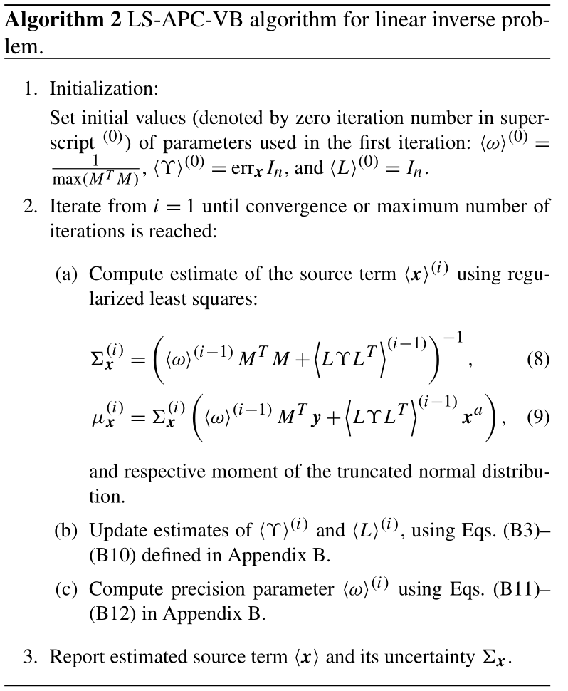
The variational Bayes' solution (Šmídl and Quinn, 2006) seeks the posterior in the specific form of conditional independence such as

$$\begin{array}{}\text{(16)}& \begin{array}{rl}& p(\mathit{x},\mathit{\upsilon },\mathbf{l},{\mathit{\psi }}_{\mathrm{1},\mathrm{\dots },n-\mathrm{1}},\mathit{\omega }|\mathit{y})\approx p(\mathit{x}\left|\mathit{y}\right)p\left(\mathit{\upsilon }\right|\mathit{y}\left)p\right(\mathbf{l}\left|\mathit{y}\right)\\ & p\left({\mathit{\psi }}_{\mathrm{1},\mathrm{\dots },n-\mathrm{1}}\right|\mathit{y}\left)p\right(\mathit{\omega }\left|\mathit{y}\right).\end{array}\end{array}$$

The best possible approximation minimizes Kullback–Leibler divergence (Kullback and Leibler, 1951) between the estimated solution and hypothetical true posterior. This minimization uniquely determines the form of the posterior distribution:

$$\begin{array}{}\text{(17)}& {\displaystyle }\stackrel{\mathrm{̃}}{p}\left(\mathit{x}\right|\mathit{y})=& {\displaystyle }t{\mathcal{N}}_{\mathit{x}}\left({\mathit{\mu }}_{\mathit{x}},{\mathrm{\Sigma }}_{\mathit{x}}\right),\text{(18)}& {\displaystyle }\stackrel{\mathrm{̃}}{p}\left({\mathit{\upsilon }}_j\right|\mathit{y})=& {\displaystyle }{\mathcal{G}}_{{\mathit{\upsilon }}_j}\left({\mathit{\alpha }}_j,{\mathit{\beta }}_j\right),\forall j=\mathrm{1},\mathrm{\dots },n,\text{(19)}& {\displaystyle }\stackrel{\mathrm{̃}}{p}\left(l_j\right|\mathit{y})=& {\displaystyle }{\mathcal{N}}_{l_j}\left({\mathit{\mu }}_{l_j},{\mathrm{\Sigma }}_{l_j}\right),\forall j=\mathrm{1},\mathrm{\dots },n-\mathrm{1},\text{(20)}& {\displaystyle }\stackrel{\mathrm{̃}}{p}\left({\mathit{\psi }}_j\right|\mathit{y})=& {\displaystyle }{\mathcal{G}}_{{\mathit{\psi }}_j}\left({\mathit{\zeta }}_j,{\mathit{\eta }}_j\right),\forall j=\mathrm{1},\mathrm{\dots },n-\mathrm{1},\text{(21)}& {\displaystyle }\stackrel{\mathrm{̃}}{p}\left(\mathit{\omega }\right|\mathit{y})=& {\displaystyle }{\mathcal{G}}_{\mathit{\omega }}\left(\mathit{\vartheta },\mathit{\rho }\right),\end{array}$$

for which the shaping parameters ${\mathit{\mu }}_{\mathit{x}},{\mathrm{\Sigma }}_{\mathit{x}},{\mathit{\alpha }}_j,{\mathit{\beta }}_j,{\mathit{\mu }}_{l_j},{\mathrm{\Sigma }}_{l_j},{\mathit{\zeta }}_j,{\mathit{\eta }}_j,\mathit{\vartheta }$, and ρ are derived in Appendix B. The shaping parameters are functions of standard moments of posterior distribution, which are denoted here as $\widehat{\mathit{x}}$ and indicate the expected value with respect to the distribution on the variable in the argument. The standard moments together with shaping parameters form a set of implicit equations solved iteratively; see Algorithm 2. Note that only convergence to a local optimum is guaranteed; hence, a good initialization and iteration strategy are beneficial (see Algorithm 2 and the discussion in Tichý et al., 2016). The algorithm is denoted as the LS-APC-VB algorithm.

2.3.2 Gibbs sampling solution

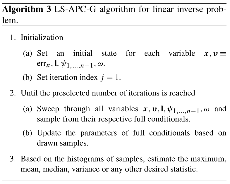
The Gibbs sampler is a Markov chain Monte Carlo method for obtaining sequences of samples from distributions for which direct sampling is difficult or intractable (Casella and George, 1992). It is a special case of the Metropolis–Hastings algorithm with the proposal distribution derived directly from the model (Chib and Greenberg, 1995). Given a joint probability density $p(\mathit{x},\mathit{\upsilon },\mathbf{l},{\mathit{\psi }}_{\mathrm{1},\mathrm{\dots },n-\mathrm{1}},\mathit{\omega },\mathit{y})$, a full conditional distribution needs to be derived for each variable or a block of variables; i.e., for x, distribution $p\left(\mathit{x}\right|\mathit{\upsilon },\mathbf{l},{\mathit{\psi }}_{\mathrm{1},\mathrm{\dots },n-\mathrm{1}},\mathit{\omega },\mathit{y})$ has to be found. These full conditionals then serve as proposal generators and have the same form as Eqs. (17)–(21). We use the original Gibbs sampler from George and McCulloch (1993). Having samples from the last iteration, or a random initialization for the first iteration, the algorithm sweeps through all variables and draws samples from their respective full conditional distributions. It can be shown that samples generated in such a manner form a Markov chain whose stationary distribution, the distribution to which the chain converges, is the original joint probability density. Since the convergence of the algorithm can be very slow, it is common practice to discard the first few obtained samples. This is known as a burn-in period. The advantage of this algorithm is its indifference to the initial state from which sampling starts.

2.4 Tuning parameters and prior source term

All mentioned methods are sensitive to a certain extent to the selection of their parameters. Here, we will identify these tuning parameters and discuss their settings in the following experiments. Moreover, we will discuss the selection of the prior source term.

The optimization approach is summarized in Algorithm 1 wherein two key tuning parameters are needed: parameter err_x, which affects the closeness of a solution to the prior source term through the matrix B, and parameter ϵ, which affects the smoothness of a solution. In the following experiments, we select the parameter ϵ by experience, while it can be seen that the solution is similar for a relatively wide range of values (a few orders of magnitude). The parameter err_x seems to be crucial for the optimization method and sensitivity to the choice of this parameter will be studied, while err_x will be referred to as the tuning parameter. Note that heuristic techniques such as the L-curve method (Hansen and O'Leary, 1993) cannot be used here because of the modification of the matrix B within the algorithm. This will be demonstrated in Sect. 3 (Fig. 2). The LS-APC-VB method, summarized in Algorithm 2, also needs the selection of initial err_x; however, relatively low sensitivity to this choice was reported (Tichý et al., 2016). The LS-APC-G method, summarized in Algorithm 3, is also initialized using err_x, while its sensitivity to this choice is negligible due to the Gibbs sampling mechanism.

To select the prior source term seems to be an even more difficult problem, especially in cases of releases with limited available information. Therefore, we will investigate various errors in the prior source term, which can be considered thanks to controlled experiments in which the true source term is available. We consider the time shift of the prior source term in contrast with the true source term, different scales, and a blurred version of the true source term. These errors can be examined alone or combined, which will probably be more realistic.

2.5 Tuning by cross-validation

While the tuning parameters selected in the previous section are often selected manually, statistical methods for their selection are also available. One of the most popular is cross-validation (Efron and Tibshirani, 1997), which we will investigate in the context of source term determination. The method is really simple: all available data are split into training and testing datasets y_train, M_train, y_test, and M_test. The training dataset is then used for source term estimation, while the test dataset is used for computation of the norm of the residue of the estimated source term, $\left|\right|{\mathit{y}}_{\text{test}}-{\mathbf{M}}_{\text{test}}〈\mathit{x}〉|{|}_{\mathrm{2}}$. Such an estimate is known to be almost unbiased but with large variance. Therefore, the procedure is repeated several times and the tuning parameters are selected based on statistical evaluation of the results. In this experiment, we repeat the random selection of 80 % of the measurements as the training set and using the remaining 20 % as the test set. For each tuning parameter err_x, this is repeated 100 times in order to reach statistical significance of the selected tuning parameter.

3 Sensitivity study on the ETEX dataset

The European Tracer Experiment (ETEX) is one of a few large controlled tracer experiments (see https://rem.jrc.ec.europa.eu/etex/, last access: 26 April 2020). We use data from the first release in which a total amount of 340 kg of nearly inert perfluoromethylcyclohexane (PMCH) was released at a constant rate for nearly 12 h at Monterfil in Brittany, France, on 23 October 1994 (Nodop et al., 1998). Atmospheric concentrations of PMCH were monitored at 168 measurement stations across Europe with a sampling interval of 3 h and a total number of measurements of 3102. The ETEX dataset has been used as a validation scenario for inverse modeling (see, e.g., Bocquet, 2007; Martinez-Camara et al., 2014; Tichý et al., 2016). The great benefit of this dataset is that the estimated source terms can be directly compared with the true release given in Fig. 1 (first row) using dashed red lines.

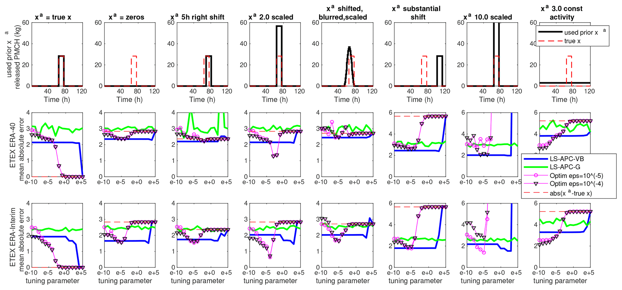
Figure 1 The uppermost row of panels shows eight different prior source terms x^a (black lines) used for the ETEX source term estimation. The true ETEX source term is repeated in every panel (red dashed line). The middle and the lowermost rows display the mean absolute error between estimated and true source terms for the ETEX ERA-40 and ETEX ERA-Interim datasets, respectively.

To calculate the SRS matrices, we used the Lagrangian particle dispersion model FLEXPART (Stohl et al., 1998, 2005) version 8.1. We assume that the release period occurred during 120 h period; thus, 120 forward calculations of a 1 h hypothetical unit release were performed and SRS coefficients were calculated from simulated concentrations corresponding to the 3102 measurements. As a result, we obtained the SRS matrix $\mathbf{M}\in {\mathbf{R}}^{\mathrm{3102}\times \mathrm{120}}$. FLEXPART is driven by meteorological input data from the European Center for Medium-Range Weather Forecasts (ECMWF) from which different datasets are available. We used two: (i) data from the 40-year reanalysis (ERA-40) and (ii) data from the continuously updated ERA-Interim reanalysis. The computed matrices for ETEX are given in Appendix C together with their associated singular values to demonstrate conditioning of the problem.

The tested method will be compared in terms of the mean absolute error (MAE) between the estimated and the true source term for different tuning parameters err_x. We select two representative values of the smoothing parameter ϵ for the optimization method. Specifically, we selected $\mathit{ϵ}={\mathrm{10}}^{-\mathrm{5}}$ and $\mathit{ϵ}={\mathrm{10}}^{-\mathrm{4}}$, while higher values lead to overly smooth and lower values to non-smooth solutions. We tested eight different prior source terms x^a; see Fig. 1, top row, black lines. These included the following: x^a equal to (i) the true source term; (ii) zeros for all elements; (iii) true source term right-shifted by five time steps; (iv) true source term scaled by a factor of 2.0; (v) true source term blurred using a convolution kernel of five time steps, left-shifted by five time steps, and scaled by a factor of 1.3; (vi) true source term substantially right-shifted; (vii) true source term scaled by a factor of 10; and (viii) source term with constant activity. The resulting MAEs for all tested methods and for all eight prior source terms are displayed in Fig. 1 for ETEX with the ERA-40 dataset in the second column and for ETEX with ERA-Interim in the third row. The figures in the second and third rows are accompanied by the MAE between the true source term and the prior source term used, displayed with dashed red lines.

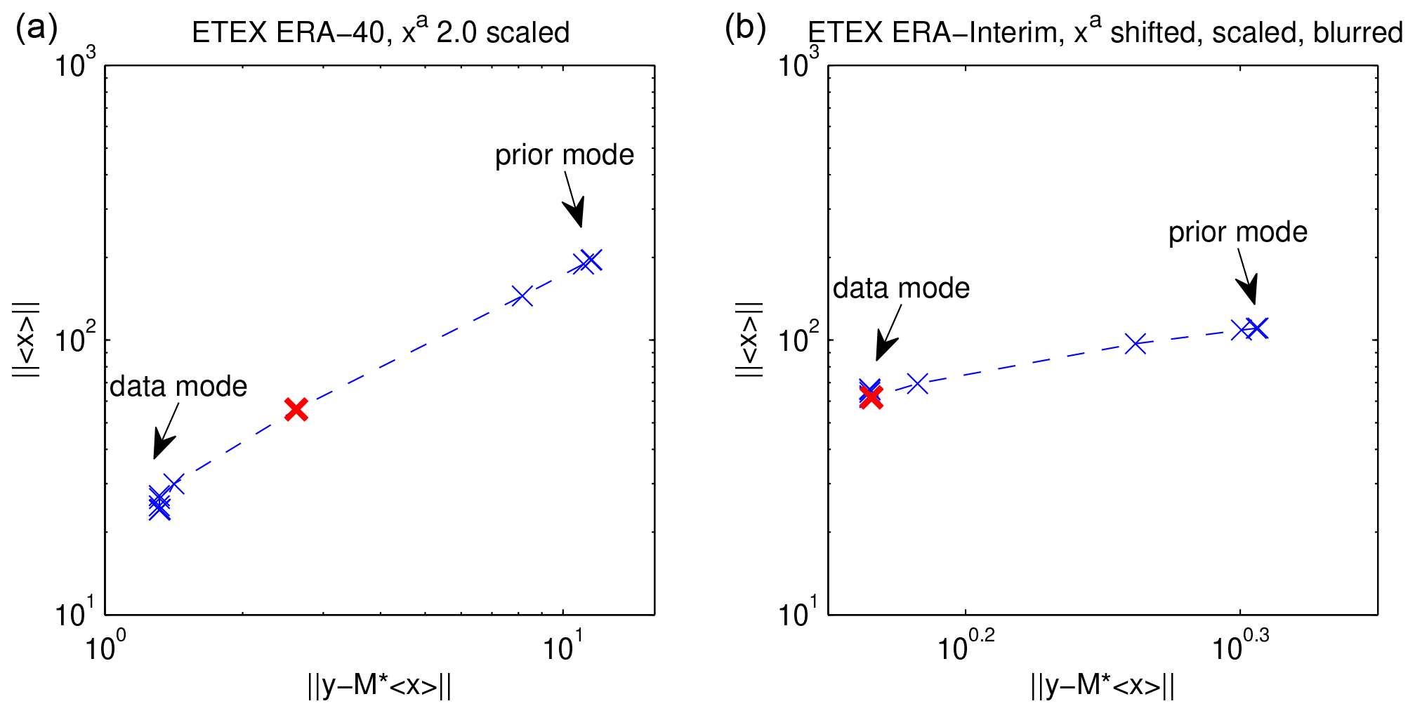
Figure 2 L-curve-type plots using the optimization algorithm with $\mathit{ϵ}=\mathrm{1}e-\mathrm{5}$ from ETEX ERA-40 with x^a 2.0 scaled (a) and from ETEX ERA-Interim with x^a shifted, scaled, and blurred (b). The red crosses denote “sweet spots”.

3.1 Results

We observe that for all choices of the optimization method, the results exhibit two notable modes of solution: the data mode for tuning parameters with minimum impact on the loss function and the prior mode for tuning parameter values that cause the prior to dominate the loss function. This is notable for the results in the range of err_x in Fig. 1. For ${\text{err}}_{\mathit{x}}={\mathrm{10}}^{-\mathrm{10}}$ the data term dominates the loss function, and all methods converge to a similar answer (note that the data mode is different for different smoothing parameters in the optimization method).

For err_x=10⁵, the loss function is dominated by the prior and all estimates converge to x^a. Although there are typically only two visibly stable modes of all the solutions (the data and prior mode), we also observe a third mode in the optimization solution, best seen, e.g., in Fig. 1 in the second row and the fourth column or in the third row and the fifth column, where the error significantly drops. These “sweet spots” are the desired locations that we hope to find by tuning of the hyper-parameters. While they are obvious when we know the ground truth, the challenge is to find them without this knowledge.

An attempt to find the optimal tuning via the L-curve method (i.e., dependence between the norm of the solution and the norm of the residuum between measurement and reconstruction) is displayed and demonstrated in two cases: ETEX ERA-40 with x^a 2.0 scaled (Fig. 2, left) and ETEX ERA-Interim with x^a shifted, scaled, and blurred (Fig. 2, right) for the optimization method with $\mathit{ϵ}={\mathrm{10}}^{-\mathrm{5}}$. In these cases (and all others), L-curve shapes were not reached at all and thus an optimum regularization parameter cannot be chosen from these plots. The red crosses denote the value corresponding to minima of MAEs. One can see that the sweet spots are on the transition between the data mode and the prior mode of solutions with no specific feature in these measures. More detailed analysis is presented in the next section.

The LS-APC-VB method also exhibits modes of solution; however, the transition between the data mode and the prior source term mode seems to be rather fast. Notably, no such transitions are observed in the case of the LS-APC-G method. This is caused by the fact that the Gibbs sampling is not sensitive to the selection of the initial state, as discussed in Sect. 2.3.2. With the exception of x^a as a constant activity (Fig. 1, eighth column), the LS-APC-VB method performs better than the optimization method when approaching the data mode of a solution. The LS-APC-G method suffers from overestimating the source term in time steps when the true source term is zero and not enough evidence is available in the data. This can clearly be seen in Figs. 3 and 4 where estimates from the LS-APC-G method are displayed using green lines; see especially the time steps between 15 and 45 h. This is closely related to the low sensitivities in SRS matrices between the 15th and 45th columns; see Fig. C1 for an illustration.

3.2 Desired optima of the estimated source term

Here, we will discuss the behavior of the methods around the regions of the tuning parameter with minimum MAE (sweet spots) observed in the case of the optimization method. Note that no such regions are observed in the case of the LS-APC-VB and LS-APC-G methods. The temporal profiles of the estimated source term at different penalization coefficients selected around two different sweet spots are displayed in Figs. 3 and 4.

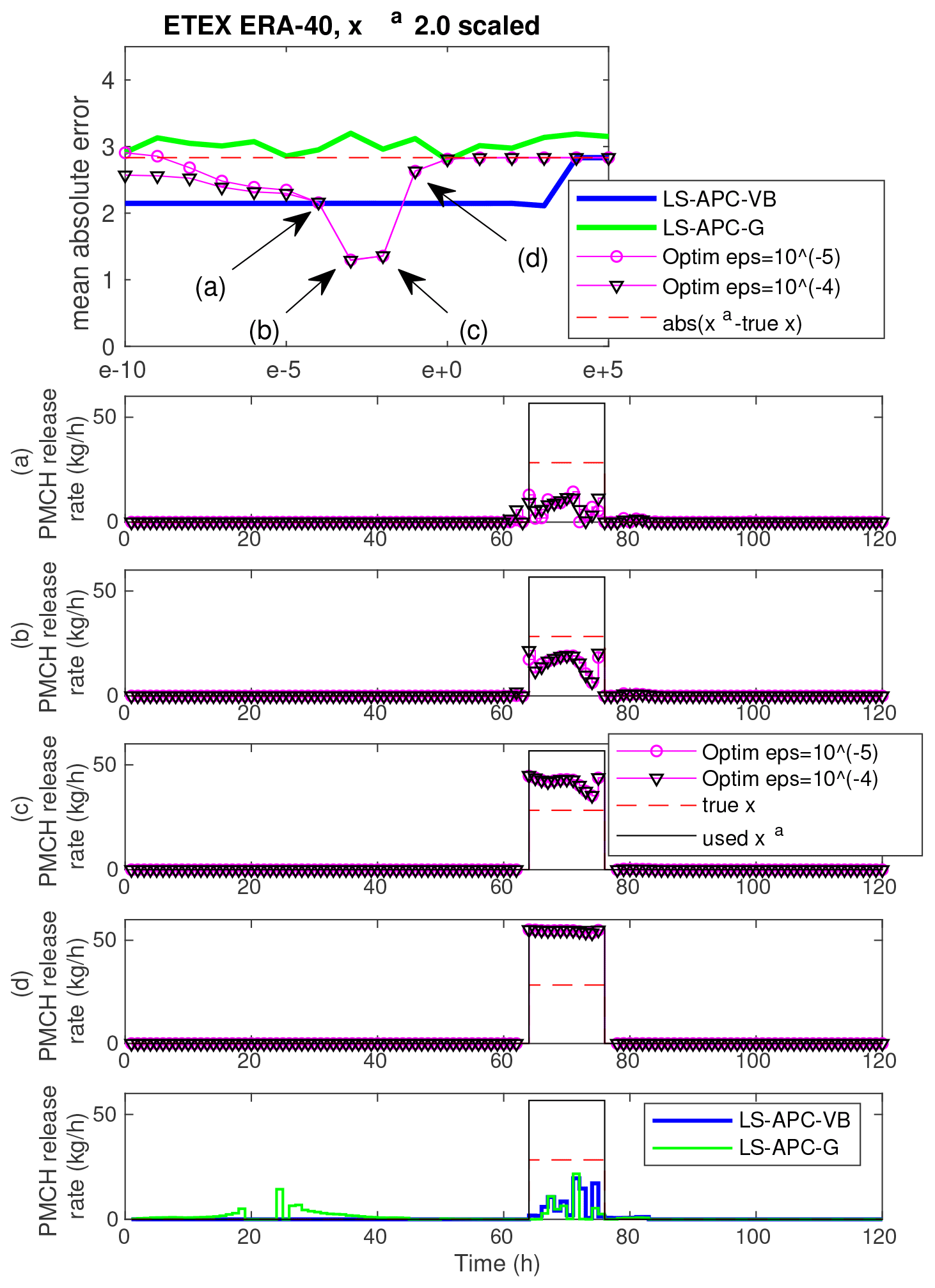
Figure 3 The uppermost panel shows mean absolute errors between estimated and true source terms for the ETEX ERA-40 dataset with x^a 2.0 scaled for all methods. Certain settings of the tuning parameter are highlighted and labeled with (a), (b), (c), and (d). Estimated source terms for these tuning parameter choices are given in the panels below. The lowermost panel displays the estimated source terms from the LS-APC-VB and LS-APC-G algorithms for comparison.

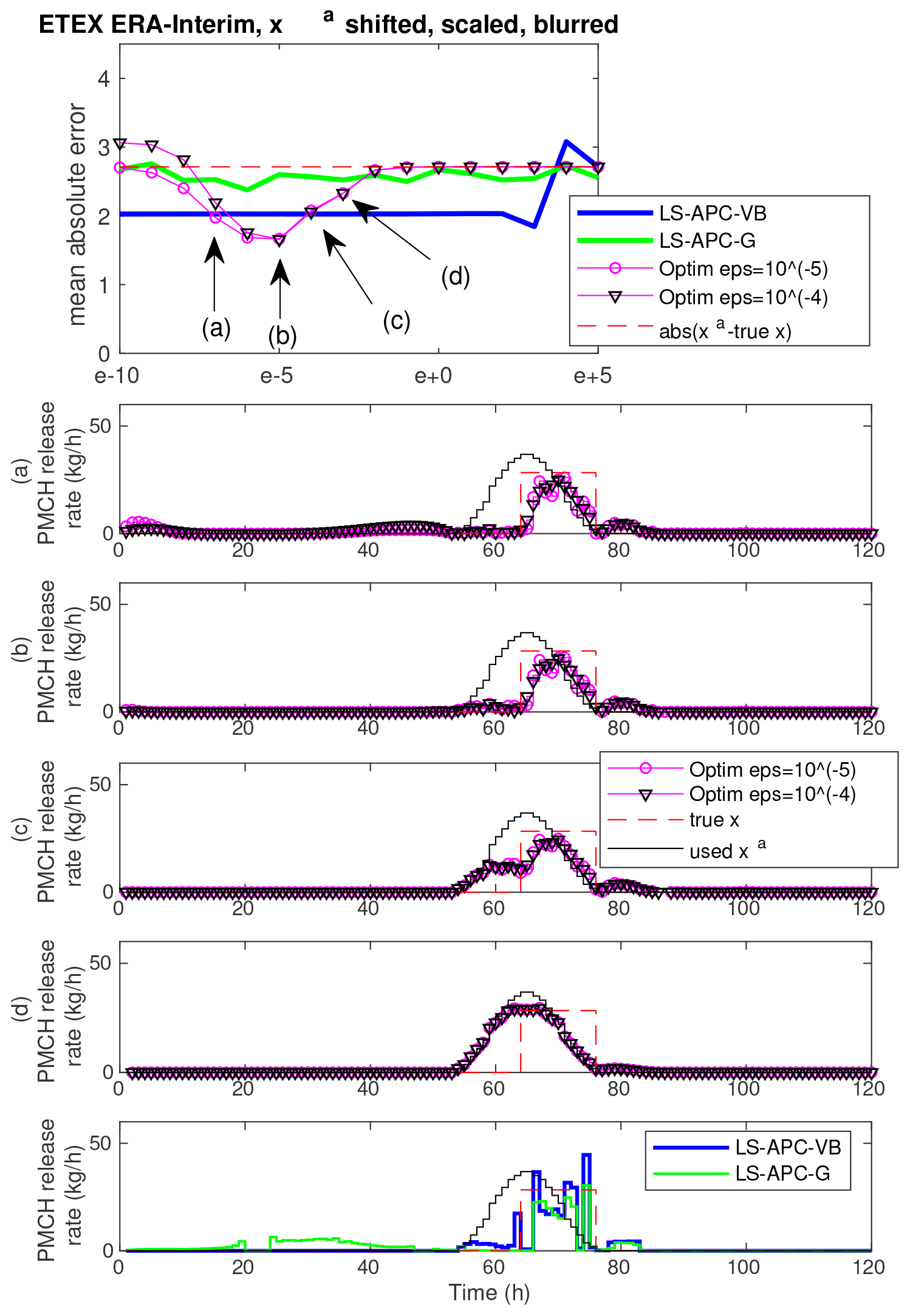
Figure 4 Same as Fig. 3 for the ETEX ERA-Interim dataset with x^a shifted, scaled, and blurred.

Figure 3 displays results for the ETEX ERA-40 dataset with the prior source term selected as the 2.0 times scaled true source term. The top graph is a copy of sensitivity to tuning in terms of MAE from Fig. 1 (second row, fourth column), and labels (a), (b), (c), and (d) indicate selected values of tuning parameters for which the resulting estimated source terms are shown in Fig. 3. The four estimates illustrate the transition from the data mode of solution (a) to the prior mode of solution (d). The data mode underestimates the true release, while the prior mode overestimates it. As displayed in Fig. 3b and c, the slow transition between these two modes allows us to approach the true source term closely, since the chosen prior term is only a scaled version of the true release and the sweet spot lies exactly between the two modes. Both the LS-APC-VB and the LS-APC-G methods diverge from the “good” solution since they consider it to be very unlikely with respect to the observed data. Since no heuristics such as the L-curve can identify this tuning as providing good results (see Fig. 2, left), we argue that choosing the optimal setting of the tuning parameter is not possible without knowledge of the true source term and the occurrence of the sweet spot is only a coincidence.

Figure 4 displays results for the ETEX ERA-Interim dataset with the prior source term shifted, scaled, and blurred in the same way as in the third row and fifth column of Fig. 3. Here, the transition is not so sharp as in the previous case since the true source term does not lie exactly on the transition between the data mode (panel a) and the prior mode (panel d). The data mode (a) also contains nonzero elements, mainly in the first half of the source term. The transition can be seen in Fig. 4b and c where the nonzero activity at the beginning of the data mode is eliminated by using prior source term information, while the nonzero elements are relatively close to the true release (b). In (c), the zero activity in the first half remains due to the prior source term; however, the estimated activity within the true release period moves toward the assumed prior source term. In (d), the estimation is already very close to the chosen prior source term. Once again, the improvement appears to be coincidental rather than systematic.

We note that the two discussed sweet spots are selected as representative cases and other observed sweet spots (see, e.g., Fig. 3, the second or eighth column) are very similar in nature. By analyzing the sweet spots, we conclude that they represent a transition from the data mode to the prior mode of solution. In some cases, the transition is very close to the true release (see, e.g., Fig. 3), while in some cases, no point on the transition path approaches the true solution (see, e.g., Fig. 4), and the data or prior mode is the closest.

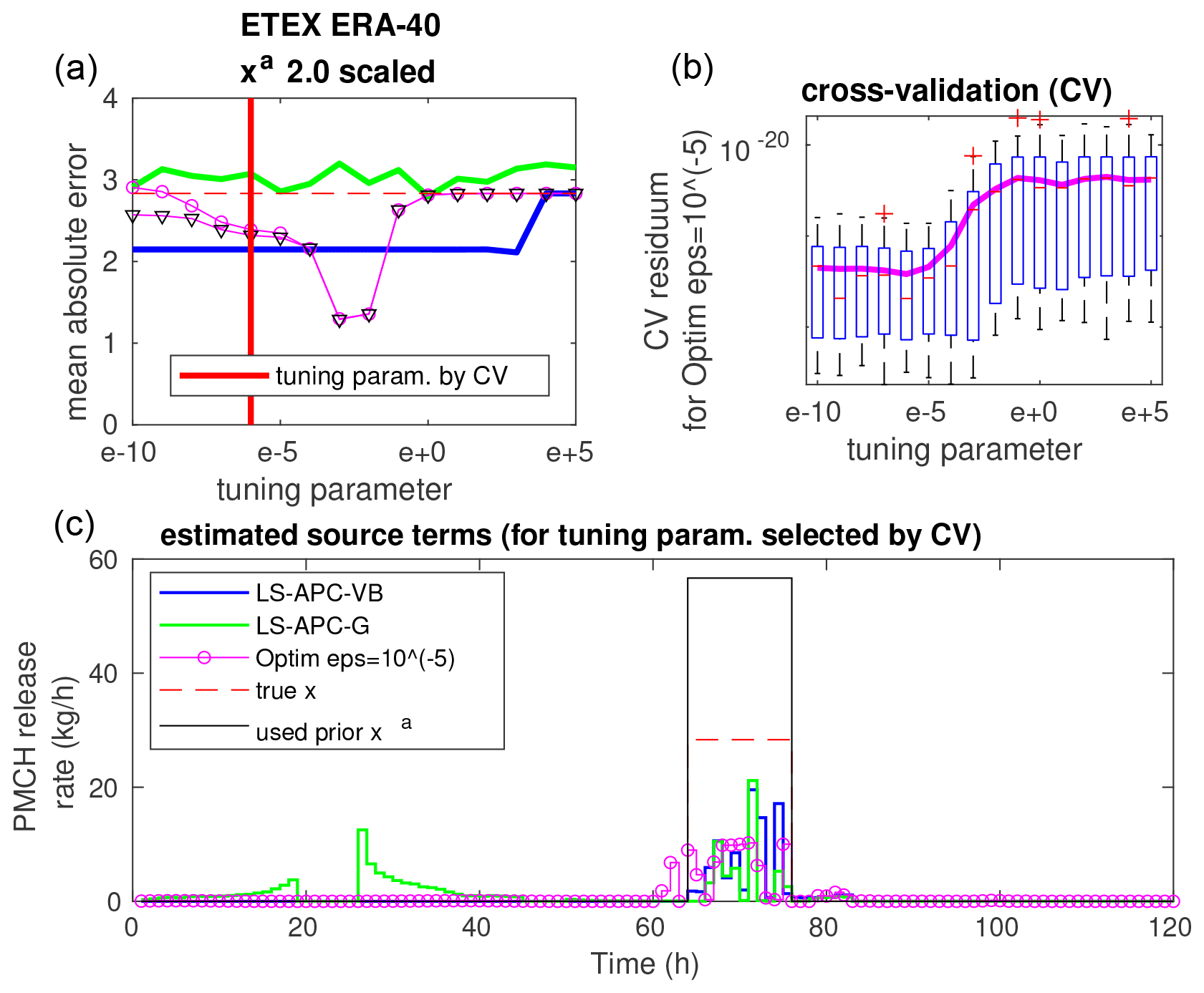
Figure 5 The top left panel (a) shows the sensitivity of MAE to the tuning parameter for the ETEX ERA-40 dataset with x^a 2.0 scaled. This is a repetition from Fig. 1. The chosen optimal setting based on CV is shown with a thick red vertical line. The top right panel (b) shows the error residuals of the CV experiments as a function of the tuning parameter. Residuals are shown as box-and-whisker plots, where the boxes extend between the 25th and 75th percentiles (whiskers between 2.7 sigmas) and medians are marked with red lines, while mean values are displayed using a solid magenta line. The lowermost panel (c) shows the source term obtained with the tuning parameter setting chosen via CV.

3.3 Tuning by cross-validation

Since the LS-APC-VB and LS-APC-G methods provide rather stable estimates of the source term, we will investigate the use of cross-validation (CV) in optimization-based approaches. The results of CV for the optimization method with $\mathit{ϵ}={\mathrm{10}}^{-\mathrm{5}}$ for selected combinations are displayed in Figs. 5, 6, and 7 in the top right panels: (i) ERA-40 with x^a 2.0 scaled; (ii) ERA-Interim with x^a shifted, blurred, and scaled; and (iii) ERA-40 with x^a equal to the true source term. The results are displayed using box plots where medians are displayed using red lines inside boxes, while the boxes cover the 25th and 75th quantiles. The mean values of the residuals for each tuning parameter are displayed using magenta lines. The value of the tuning parameter that minimizes the CV error is also visualized in the top left panels using solid vertical red lines inside the graphs of MAE sensitivity from Fig. 1. Bottom panels of figures display the estimated source terms using the tested methods for the tuning parameter selected by cross-validation together with the true source term (dashed red line) and the prior source term used (full black line).

Figure 6 Same as Fig. 5 for the ETEX ERA-Interim dataset with x^a shifted, scaled, and blurred.

Figure 7 Same as Fig. 5 for the ETEX ERA-40 dataset with x^a equal to the true source term.

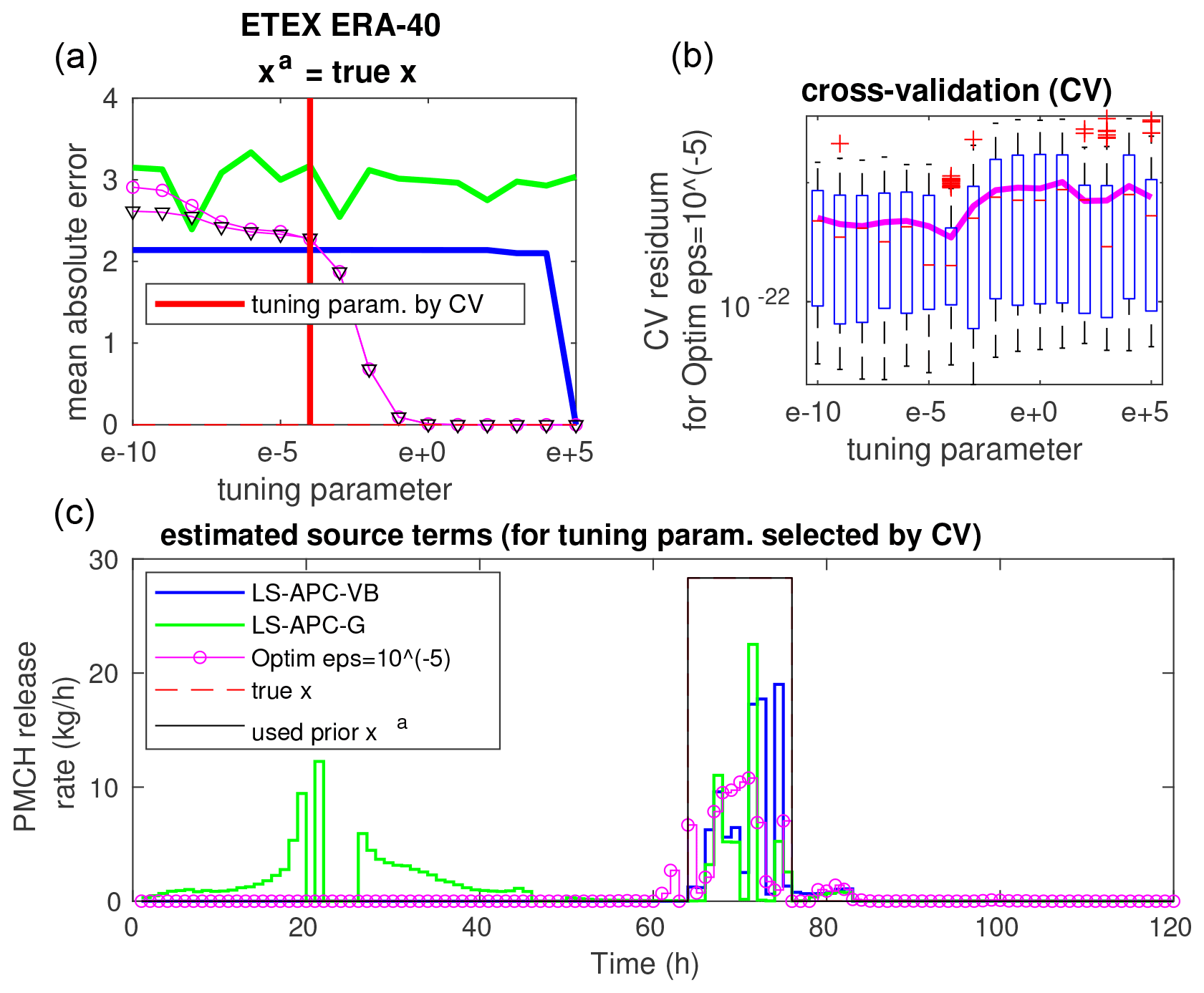
The results demonstrate significant differences between the prior mode and the data mode of the solution, which can be seen in all cross-validation box plots. This is also the case for x^a, which is not displayed here. Notably, the minima of cross-validation are not reached in the positions of the sweet spots, indicating that the observed MAE minima are coincidental. In all tested cases, the minima of cross-validation are reached closer to the data mode than to the prior mode. This is demonstrated for the extreme case of x^a equal to the true source term in Fig. 7. Even for this case, the minimum of cross-validation is associated with the data mode rather than the prior mode.

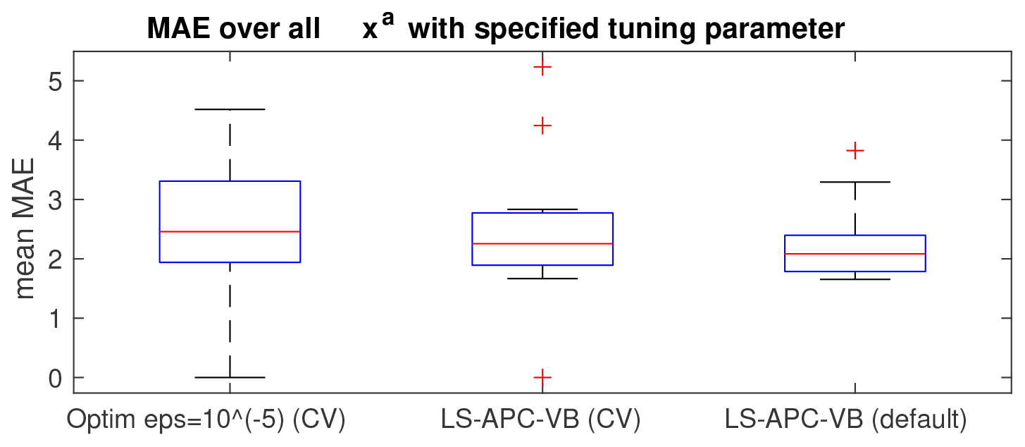
Figure 8 Box-and-whisker plots of the MAE averaged over all explored prior source terms, with the tuning parameter settings determined by CV for the optimization method (left) and the LS-APC-VB method (middle), as well as for the LS-APC-VB method using a default err_x setting of 10⁰.

To evaluate the overall results, we compute the mean MAE over all estimated source terms using the optimization method with $\mathit{ϵ}={\mathrm{10}}^{-\mathrm{5}}$ and the tuning parameter err_x selected using cross-validation (CV) for each prior source term x^a. This result is given in Fig. 8 using a box-and-whisker plot. The same box-and-whisker plots are also computed for the LS-APC-VB method with the same scheme of selection of tuning parameters err_x using the cross-validation method (denoted CV in Fig. 8) and for the LS-APC-VB algorithm with the tuning parameter err_x set to 10⁰ as recommended in Tichý et al. (2016) (denoted default in Fig. 8). These results suggest that the LS-APC-VB method with fixed start (but weighted to data using selection of ω⁽⁰⁾) slightly outperforms other methods in terms of the mean MAE for ETEX data with various assumed prior source terms without the necessity of exhaustive tuning.

4 Sensitivity study on the Chernobyl dataset

We demonstrate the sensitivity of the tuning methods to estimation of the source term for the Chernobyl accident, which became, together with the Fukushima accident, a widely discussed case in the inverse modeling literature. Specifically, we study caesium-134 (Cs-134) and caesium-137 (Cs-137) releases from the Chernobyl nuclear power plant (ChNPP). For this purpose, we use a recently published dataset (Evangeliou et al., 2016) consisting of 4891 observations of Cs-134 and 12 281 observations of Cs-137. We use the same experimental setup as in Evangeliou et al. (2017), which will now briefly be described.

4.1 Atmospheric modeling

The Lagrangian particle dispersion model FLEXPART version 10.3 (Stohl et al., 1998, 2005; Pisso et al., 2019) was used to simulate the transport of radiocesium and to calculate the SRS matrices. FLEXPART was driven by two meteorological reanalyses so that these can be compared. First, ERA-Interim (Dee et al., 2011), a European Center for Medium-Range Weather Forecast (ECMWF) reanalysis, was used with a temporal resolution of 3 h and spatial resolution of circa 80 km on 60 vertical levels from the surface up to 0.1 hPa. Second, the ERA-40 (Uppala et al., 2005) ECMWF reanalysis was used at a 125 km spatial resolution. The emissions from the ChNPP are discretized into six 0.5 km high vertical layers from 0 to 3 km. The assumed temporal resolution is 3 h from 00:00 UTC on 26 April to 21:00 UTC on 5 May 1986, for which the forward runs of FLEXPART are done. This period is selected according to the consensus that the activity declined by approximately 6 orders of magnitude after 5 May (De Cort et al., 1998). This discretized the temporal–spatial domain to 480 assumed releases (80 temporal elements times 6 vertical layers) for each nuclide. For each spatiotemporal element, concentration and deposition sensitivities are computed using 300 000 particles. Following Evangeliou et al. (2017), the aerosol tracers Cs-134 and Cs-137 are subject to wet (Grythe et al., 2017) and dry (Stohl et al., 2005) deposition depending on different particle sizes with aerodynamic mean diameters of 0.4, 1.2, 1.8, and 5.0 µm. The distribution of mass is assumed as 15 %, 30 %, 40 %, and 15 % for 0.4, 1.2, 1.8, and 5.0 µm particle sizes, respectively, following measurements of Malá et al. (2013) and computation results of Tichý et al. (2018).

4.2 Prior source term and measurement uncertainties

The exact temporal profile of the Chernobyl release is uncertain, although certain features are commonly accepted (De Cort et al., 1998). The first 3 d correspond to higher release with an initial explosion and release of part of the fuel. The next 4 d correspond to lower releases, and the last 3 d correspond to higher releases again due to fires and core meltdown. After these 10 d, the released activity dropped by several orders of magnitude (De Cort et al., 1998).

We follow the setup of Evangeliou et al. (2017) and consider six previously estimated Chernobyl source terms of Cs-134 and Cs-137 for which the criteria of consideration were their sufficient temporal resolution and emission height information. The source terms are taken from Brandt et al. (2002) (two cases with the same amount of release but slightly different release heights), Persson et al. (1987), Izrael et al. (1990), Abagyan et al. (1986), and Talerko (2005). See Evangeliou et al. (2017) for detailed descriptions and profiles. The prior source term in our experiment is computed as their average emissions at a given time and height. In sum, the total prior releases of Cs-134 and Cs-137 are 54 and 74 PBq, respectively.

The uncertainties associated with measurements are relatively high since both concentration and deposition measurements are used from the dataset (Evangeliou et al., 2016). As was pointed out by Gudiksen et al. (1989) and Winiarek et al. (2014), deposition measurements may be biased by an unknown mass of radiocesium already deposited over Europe from, e.g., nuclear weapons tests. This mass has, however, been reported (De Cort et al., 1998) and already subtracted from the dataset. Still, similarly to Evangeliou et al. (2017), we consider relative measurement errors of 30 % for concentration measurements and 60 % for deposition measurements, while the absolute measurement errors are handled in the same way as in Stohl et al. (2012). Here, the measurement vector and SRS matrix are preconditioned (scaled) using the matrix R, which is a diagonal matrix with ${\left({\mathit{\sigma }}_{\text{abs}}^{\mathrm{2}}+{\left({\mathit{\sigma }}_{\text{rel}}\circ \mathit{y}\right)}^{\mathrm{2}}\right)}^{-\mathrm{1}/\mathrm{2}}$ on its diagonal, where σ_abs is assumed absolute error, σ_rel is assumed relative error, and ∘ denotes the Hadamard product (element-wise multiplication). The scaling is then y_scaled=Ry and M_scaled=RM.

4.3 Results

In this case, direct comparison of the estimates with the true emission profile is not possible since this remains unknown. Therefore, we will provide results of the tested methods as the sensitivity of the total estimated release activity to tuning parameters in the same way as in Sect. 3. Note that the total release activity is a sum of releases from all six vertical layers and all four aerosol size fractions. Due to this composition of the problem, the selection of the smoothness parameter ϵ in the case of the optimization approach is relatively difficult since specific selection may fit better for one vertical layer than for another. We will provide results for two settings of this parameter, $\mathit{ϵ}={\mathrm{10}}^{-\mathrm{2}}$ and $\mathit{ϵ}={\mathrm{10}}^{-\mathrm{4}}$, leading to two different behaviors of the optimization method.

Figure 9 Estimated total released activities for both meteorological reanalyses (ERA-40 and ERA-Interim) and both nuclides (Cs-134 and Cs-137) using all tested methods; see the label bar on the right for a line description.

The resulting estimates of the total released activity are displayed in Fig. 9 where the total of the prior source term used x^a is displayed with a dashed red line (same for all tested settings of the tuning parameter err_x). The estimated total release activity with the use of the prior source term x^a is displayed using full lines with colors given in the legend in Fig. 9, while estimations without the use of this prior source term, i.e., with x^a=0, are given using dashed lines and respective colors.

Similarly to the ETEX results, the results in Fig. 9 suggest the occurrence of two main modes of solution, the data mode and the prior mode, with a smooth transition between them in the case of the LS-APC-VB and optimization methods. The LS-APC-G method (evaluated only at four points denoted by green squares due to high computational costs) has, again, low sensitivity to the initialization of the tuning parameter. However, the results of the LS-APC-G method are close to the data mode of the remaining method, or higher than those. Contrary to the previous results, the LS-APC-VB algorithm does not provide a stable solution and suffers from the need to select the tuning parameter. This signifies that the problem is ill-conditioned even with the proposed regularization term; thus, VB converges to various local minima. The optimization method with both settings of the smoothness parameter also has two modes of solution. In the prior mode of solution (higher values of the tuning parameter), both settings approach the same total release activity for both nonzero (full lines) and zero (dashed lines) prior source terms. The prior mode is dominated by the prior source term used for an arbitrary smoothness parameter ϵ. The difference can be seen in the data mode whereby about one-third higher total released activity was estimated for smoothness parameter $\mathit{ϵ}={\mathrm{10}}^{-\mathrm{4}}$ than for smoothness parameter $\mathit{ϵ}={\mathrm{10}}^{-\mathrm{2}}$ on the same level of tuning parameter err_x. This is caused by the penalization of high peaks of activity in the case of $\mathit{ϵ}={\mathrm{10}}^{-\mathrm{2}}$. Thus, in the data mode of solution, the smoothness parameter is much more important than the prior source term used, which plays almost no role here.

Notice that the estimated mass is higher in the data mode than in the prior mode. This means that the model constrained by the measurement data alone would support a higher total release amount than the a priori source term. The true source term is not known; however, it is likely that the data mode overestimates the true total release. This can happen when the SRS matrix is biased. For instance, removal of radiocesium that is too rapid would lead to estimated air concentrations with the correct source term that are too low, and the inversion would compensate for the bias by increasing the posterior source term (notice, though, that deposition values would in this case be overestimated at least close to the source, leading to the contrary effect for the deposition data). Regardless, this effect shows that in the data mode, the resulting source term is heavily influenced by possible biases in the transport model.

Figure 10 Cross-validation for Chernobyl Cs-134 (top panels) and Cs-137 (bottom panels) source terms using FLEXPART driven with ERA-40 meteorological reanalyses. Optima in the sense of cross-validation are denoted using red circles with total estimated releases reported in the legends.

4.4 Tuning by cross-validation

The same cross-validation scheme as in the case of ETEX (Sect. 3.3) was used here for the Chernobyl datasets. The train–test split was once again 80 %–20 %, and the CV was performed 50 times for each tuning parameter err_x. The cross-validation errors are displayed in Fig. 10 using box plots and associated mean values of the residue errors $\left|\right|{\mathit{y}}_{\text{test}}-{\mathbf{M}}_{\text{test}}〈\mathit{x}〉|{|}_{\mathrm{2}}$. Here, the results are given for the datasets of Cs-134 (top row) and Cs-137 (bottom row) with FLEXPART driven with ERA-40 meteorological fields. We will investigate CV for the tuning of parameters for the optimization and the LS-APC-VB method. The results are presented for two x^a configurations in Fig. 10: LS-APC-VB with x^a, LS-APC-VB with x^a=0, the optimization method with x^a and with smoothness parameter $\mathit{ϵ}={\mathrm{10}}^{-\mathrm{2}}$, and the optimization method with x^a=0 and with smoothness parameter $\mathit{ϵ}={\mathrm{10}}^{-\mathrm{2}}$. For these, box plots are displayed together with mean residuals using the same types of lines as in Fig. 9. Moreover, minimal mean residuals are identified and denoted using red circles in Fig. 10 for each graph, and their associated total activities are displayed in the legend of each graph.

In the case of Cs-134 (top row), the cross-validation was able to determine optimal values of tuning parameters in the case of all tested methods. The total estimated releases associated with these tuning parameters are 87.1 PBq (LS-APC-VB with x^a), 56 PBq (LS-APC-VB with x^a=0), 69.7 PBq (the optimization method with x^a), and 43 PBq (the optimization method with x^a=0), which are in accordance with the mean of previously reported total activity of 54 PBq used as a prior. Note that the prior-dominated modes have lower residuals than the data-dominated modes in all cases. This suggests that the prior source term used and applied to the FLEXPART/ERA-40 simulation matches the measurements well. On the other hand, this is not the case for Cs-137 for which the prior-dominated modes have, with the exception of LS-APC-VB with x^a=0, significantly higher residuals than the data-dominated modes. This may be caused by two factors. First, the prior source term is less adequate for interpretation of measurements of Cs-137 than those of Cs-134. Second, all methods assume a quadratic loss function, which may be less appropriate for this dataset and could cause overestimation of the source term with the tuning parameter selected using cross-validation in comparison with the previously reported 74 PBq used as a prior. We note that similar results were also observed with the ERA-Interim dataset.

The results suggest that a well-selected prior source term can bind the solution to acceptable values and prevent the occurrence of extreme outliers. On the other hand, we observed that the regularization terms commonly used to compensate for errors of the SRS matrices are not able to compensate for the error caused by inaccurate SRS matrices. Further research is clearly needed to develop a more relevant method of regularization.

5 Conclusions

Methods for the determination of the source term of an atmospheric release have to cope with inaccurate prediction models often represented by the source–receptor sensitivity (SRS) matrix. Relying solely on the SRS matrix using a best estimate of weather and dispersion parameters may lead to highly inaccurate results. We have shown that various regularization terms introduced by different inversion methods are essentially coarse approximations of the error of the SRS matrix, and thus we can evaluate their suitability using methods of statistical model validation. We have performed sensitivity tests of inverse modeling methods to the selection of the prior source term (first guess) and other tuning parameters for two selected inversion methods: the optimization method (Eckhardt et al., 2008) and the LS-APC method (Tichý et al., 2016). These were preformed on datasets from the ETEX controlled release and the Chernobyl releases of caesium-134 and caesium-137.

We have observed that the results have two strong modes of solution: the data mode for minimal influence of the prior on the loss and the prior mode for the loss function with significant influence of the prior. The prior mode is naturally significantly influenced by the choice of the prior source term. However, the dominant impact on the resulting estimate has the choice of the regularization. In the case of the ETEX dataset, good estimates were obtained for every choice of the prior source term; however, the regularization has to be carefully tuned. For some choices of the prior source term, the error of the estimated source term was exceptionally low for good selection of the tuning parameters. After analyzing these minima, we conjecture that they are caused by coincidence. These minima are visible only in comparison with the ground truth; they have no visible impact on the common validation metrics such as the L-curve or cross-validation and thus cannot be objectively identified.

We have tested the suitability of the cross-validation approach for selection of the tuning parameters for both methods. In the case of the ETEX release, we have observed that this approach tends to select modes closer to the data mode than the prior mode of solution. However, this is not the case of the Chernobyl Cs-134 release for which cross-validation selects solutions close to the prior-dominated mode. This may be caused by the fact that the prior source term used here fits the measurements well, and only small corrections by the inversion are needed. An interesting question is whether it is beneficial to use a nonzero prior source term at all. Considering ETEX, for which the true release is known, one can see that the estimates in data modes are often even better than the considered prior source terms. On the other hand, when the prior source term used is close to the true release, which is probably the case for the Chernobyl Cs-134 release, its use seems beneficial. Also, the prior source term could be valuable in cases when the release is not fully seen by the measurement network and thus the measurements do not provide a good constraint for the source term estimation. However, determining the reliability of the prior source term is difficult and even impossible in real-world scenarios, and the prior source term would probably be shifted, scaled, and/or blurred. We recommend tackling this task using the cross-validation approach, providing a reasonable although computationally expensive tool for determination at least between a prior-dominated mode or a data-dominated mode of solution. A more sophisticated approach is to design a different regularization of the error term Δ_M exploiting, e.g., sensitivities to local changes in concentrations around the measuring sites. The information about sensitivity is already available from an atmospheric transport model but it is not fully exploited with current source term determination methods.

Appendix A: Derivation of residuum between measurement and reconstruction

From Eq. (2), $\mathit{y}=\left(\mathbf{M}+{\mathrm{\Delta }}_{\mathbf{M}}\right)\mathit{x}$ can be rewritten using the subtraction of Mx^a and Δ_Mx^a from both sides, yielding

$$\begin{array}{}\text{(A1)}& \mathit{y}-\mathbf{M}{\mathit{x}}^a-{\mathrm{\Delta }}_{\mathbf{M}}{\mathit{x}}^a=\mathbf{M}\left(\mathit{x}-{\mathit{x}}^a\right)+{\mathrm{\Delta }}_{\mathbf{M}}\left(\mathit{x}-{\mathit{x}}^a\right),\end{array}$$

which can be read as

$$\begin{array}{}\text{(A2)}& \stackrel{\mathrm{‾}}{\mathit{y}}=\mathbf{M}\stackrel{\mathrm{‾}}{\mathit{x}}+{\mathrm{\Delta }}_{\mathbf{M}}\stackrel{\mathrm{‾}}{\mathit{x}}+{\mathrm{\Delta }}_{\mathbf{M}}{\mathit{x}}^a\end{array}$$

for commonly used substitutions $\stackrel{\mathrm{‾}}{\mathit{y}}=\mathit{y}-\mathbf{M}{\mathit{x}}^a$ and $\stackrel{\mathrm{‾}}{\mathit{x}}=\mathit{x}-{\mathit{x}}^a$. This means that the minimization of Eq. (A2) is equivalent to the minimization of the former Eq. (2). Thus,

$$\begin{array}{ll}{\displaystyle }& {\displaystyle }\underset{\mathit{x}}{min}\left|\right|\mathit{y}-\mathbf{M}\mathit{x}-{\mathrm{\Delta }}_{\mathbf{M}}\mathit{x}|{|}_{\mathrm{2}}^{\mathrm{2}}⟺\underset{\mathit{x}}{min}||\stackrel{\mathrm{‾}}{\mathit{y}}\\ {\displaystyle }& {\displaystyle }-\mathbf{M}\stackrel{\mathrm{‾}}{\mathit{x}}-{\mathrm{\Delta }}_{\mathbf{M}}\stackrel{\mathrm{‾}}{\mathit{x}}-{\mathrm{\Delta }}_{\mathbf{M}}{\mathit{x}}^a|{|}_{\mathrm{2}}^{\mathrm{2}}=\\ {\displaystyle }& {\displaystyle }=\underset{\mathit{x}}{min}\left(\underset{\left|\right|\stackrel{\mathrm{‾}}{\mathit{y}}-\mathbf{M}\stackrel{\mathrm{‾}}{\mathit{x}}|{|}_{\mathrm{2}}^{\mathrm{2}}}{\underbrace{{\stackrel{\mathrm{‾}}{\mathit{y}}}^T\stackrel{\mathrm{‾}}{\mathit{y}}-\mathrm{2}{\stackrel{\mathrm{‾}}{\mathit{y}}}^T\mathbf{M}\stackrel{\mathrm{‾}}{\mathit{x}}+{\stackrel{\mathrm{‾}}{\mathit{x}}}^T{\mathbf{M}}^T\mathbf{M}\stackrel{\mathrm{‾}}{\mathit{x}}}}\right.\\ {\displaystyle }& {\displaystyle }-\mathrm{2}\underset{\text{linear in }\stackrel{\mathrm{‾}}{\mathit{x}}}{\underbrace{\left({\stackrel{\mathrm{‾}}{\mathit{y}}}^T{\mathrm{\Delta }}_{\mathbf{M}}-{\left({\mathrm{\Delta }}_{\mathbf{M}}{\mathit{x}}^a\right)}^T\mathbf{M}-{\left({\mathrm{\Delta }}_{\mathbf{M}}{\mathit{x}}^a\right)}^T{\mathrm{\Delta }}_{\mathbf{M}}\right)\stackrel{\mathrm{‾}}{\mathit{x}}}}\\ {\displaystyle }& {\displaystyle }\left.+{\stackrel{\mathrm{‾}}{\mathit{x}}}^T\underset{\mathrm{\Phi }}{\underbrace{\left({\mathbf{M}}^T{\mathrm{\Delta }}_{\mathbf{M}}+{\mathrm{\Delta }}_{\mathbf{M}}^T\mathbf{M}+{\mathrm{\Delta }}_{\mathbf{M}}^T{\mathrm{\Delta }}_{\mathbf{M}}\right)}}\stackrel{\mathrm{‾}}{\mathit{x}}\right),\end{array}$$

where terms independent of $\stackrel{\mathrm{‾}}{\mathit{x}}$ are omitted.

Appendix B: Shaping parameters of LS-APC-VB posteriors

$$\begin{array}{ll}\text{(B1)}& {\displaystyle }{\mathrm{\Sigma }}_{\mathit{x}}=& {\displaystyle }{\left(〈\mathit{\omega }〉M^{T}M+〈L\mathrm{{\rm Y}}{L}^T〉\right)}^{-\mathrm{1}},\text{(B2)}& {\displaystyle }{\mathit{\mu }}_{\mathit{x}}=& {\displaystyle }{\mathrm{\Sigma }}_{\mathit{x}}\left(〈\mathit{\omega }〉M^T\mathit{y}+〈L\mathrm{{\rm Y}}{L}^T〉{\mathit{x}}^a\right),\text{(B3)}& {\displaystyle }\mathit{\alpha }=& {\displaystyle }{\mathit{\alpha }}_{\mathrm{0}}+{\displaystyle \frac{\mathrm{1}}{\mathrm{2}}}{\mathbf{1}}_{n,\mathrm{1}},\text{(B4)}& {\displaystyle }\mathit{\beta }=& {\displaystyle }{\mathit{\beta }}_{\mathrm{0}}+{\displaystyle \frac{\mathrm{1}}{\mathrm{2}}}\mathrm{diag}\left(〈L^T\mathit{x}{\mathit{x}}^{T}L〉\right)\text{(B5)}& {\displaystyle }& {\displaystyle }-\mathrm{diag}\left(〈L^T{\mathit{x}}^a{\mathit{x}}^{T}L〉\right)+{\displaystyle \frac{\mathrm{1}}{\mathrm{2}}}\mathrm{diag}\left(〈L^T{\mathit{x}}^a{\mathit{x}}^{aT}L〉\right),\text{(B6)}& {\displaystyle }{\mathrm{\Sigma }}_{l_j}=& {\displaystyle }{\left(〈{\mathit{\upsilon }}_j〉〈x_{j+\mathrm{1}}^{\mathrm{2}}〉+〈{\mathit{\psi }}_j〉\right)}^{-\mathrm{1}},\text{(B7)}& {\displaystyle }{\mathit{\mu }}_{l_j}=& {\displaystyle }{\mathrm{\Sigma }}_{l_j}(-〈{\mathit{\upsilon }}_j〉〈x_j{x}_{j+\mathrm{1}}〉+(-\mathrm{1})〈{\mathit{\psi }}_j〉\text{(B8)}& {\displaystyle }& {\displaystyle }+{〈\mathrm{{\rm Y}}〉}_{j,j}\left({\mathit{x}}_j^a{〈\mathit{x}〉}_{j+\mathrm{1}}+{\mathit{x}}_{j+\mathrm{1}}^a{〈\mathit{x}〉}_j-{\mathit{x}}_j^a{\mathit{x}}_j^a\right)),\text{(B9)}& {\displaystyle }{\mathit{\zeta }}_j=& {\displaystyle }{\mathit{\zeta }}_{\mathrm{0}}+{\displaystyle \frac{\mathrm{1}}{\mathrm{2}}},\text{(B10)}& {\displaystyle }{\mathit{\eta }}_j=& {\displaystyle }{\mathit{\eta }}_{\mathrm{0}}+{\displaystyle \frac{\mathrm{1}}{\mathrm{2}}}〈(l_j-l_{\mathrm{0}}{)}^{\mathrm{2}}〉,\text{(B11)}& {\displaystyle }\mathit{\vartheta }=& {\displaystyle }{\mathit{\vartheta }}_{\mathrm{0}}+{\displaystyle \frac{p}{\mathrm{2}}},{\displaystyle }\mathit{\rho }=& {\displaystyle }{\mathit{\rho }}_{\mathrm{0}}+{\displaystyle \frac{\mathrm{1}}{\mathrm{2}}}\mathrm{tr}\left(〈\mathit{x}{\mathit{x}}^T〉M^{T}M\right)-{\displaystyle \frac{\mathrm{1}}{\mathrm{2}}}\mathrm{2}{\mathit{y}}^{T}M〈\mathit{x}〉\\ \text{(B12)}& {\displaystyle }& {\displaystyle }+{\displaystyle \frac{\mathrm{1}}{\mathrm{2}}}{\mathit{y}}^T\mathit{y}.\end{array}$$

Appendix C: SRS matrices used for the ETEX and Chernobyl experiments

SRS matrices for ETEX are displayed in Fig. C1 for illustration. The SRS matrix computed using ERA-40 reanalyses is in the left column, while the SRS matrix computed using ERA-Interim is in the right column. The matrices are associated with their singular values displayed in the bottom row. These illustrate properties of the matrices and, importantly, their ill conditionality.

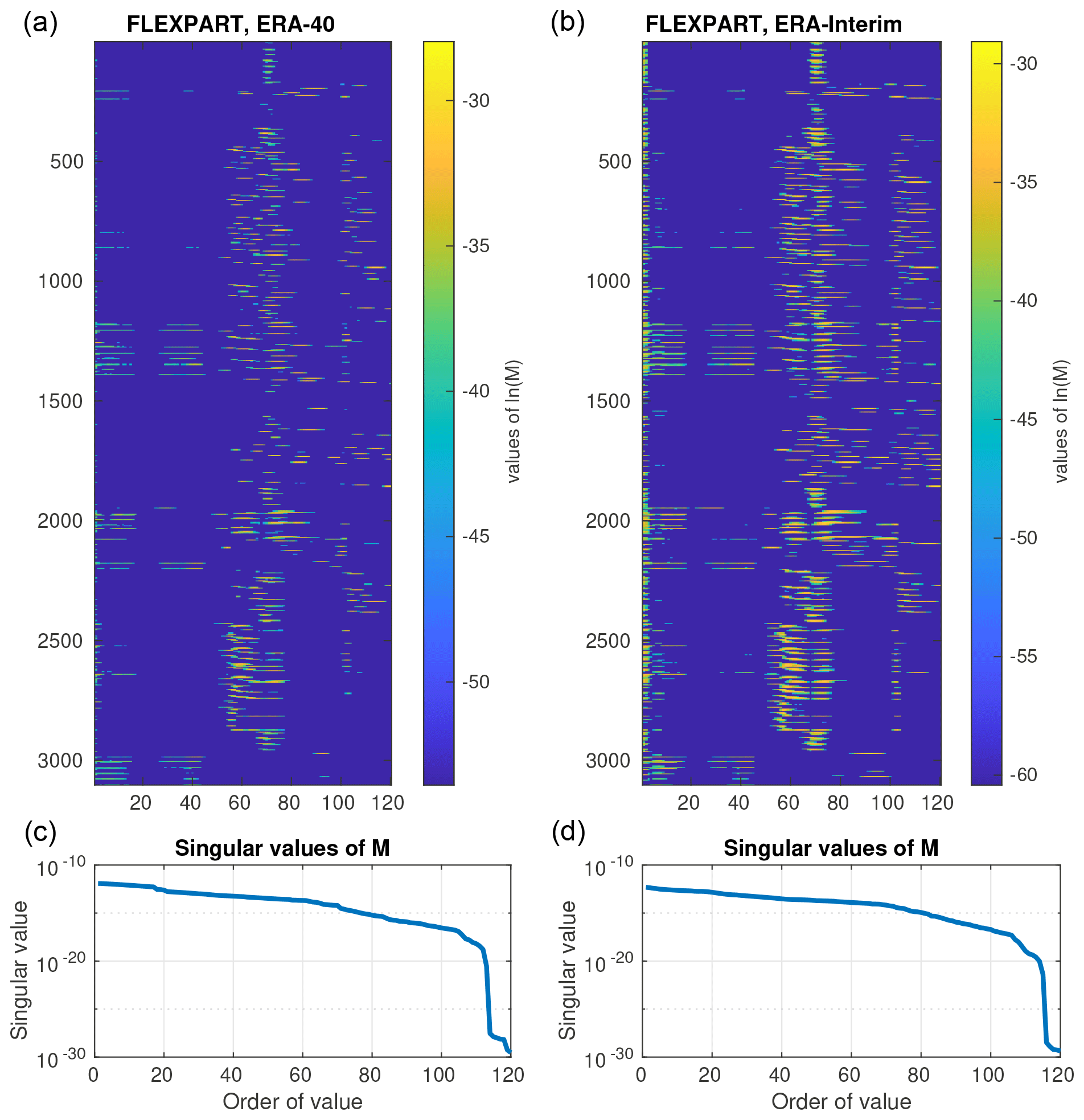
Figure C1 ETEX SRS matrices computed using FLEXPART driven by meteorological input data from the European Center for Medium-Range Weather Forecasts (ECMWF). (a, c) Data from the 40-year reanalysis (ERA-40) and (b, d) data from the continuously updated ERA-Interim reanalysis. The matrices are associated with their singular values (bottom row).