Development of a semi-Lagrangian advection scheme for the NEMO ocean model (3.1)

As resolutions of ocean circulation models increase, the advective Courant number – the ratio between the distance travelled by a fluid parcel in one time step and the grid size – becomes the most stringent factor limiting model time steps. Some atmospheric models have escaped this limit by using an implicit or semi-implicit semi-Lagrangian formulation of advection, which calculates materially conserved fluid properties along trajectories which follow the fluid motion and end at prescribed grid points. Unfortunately, this formulation is not straightforward in ocean contexts, where the irregular, interior boundaries imposed by the shore and bottom orography are incompatible with traditional trajectory calculations.

This work describes the adaptation of the semi-Lagrangian method as an advection module for an operational ocean model. We solve the difficulties of the ocean's internal boundaries by calculating parcel trajectories using a time-exponential formulation, which ensures that all parcel trajectories remain inside the ocean domain despite strong accelerations near the boundary. Additionally, we derive this method in a way that is compatible with the leapfrog time-stepping scheme used in the NEMO-OPA (Nucleus for European Modelling of the Ocean, Océan Parallélisé) ocean model, and we present simulation results for a simplified test case of flow past a model island and for 10-year free runs of the global ocean on the quarter-degree ORCA025 grid.

1 Introduction

Recent work by Smith et al. (2018) has shown that over the medium term (up to 7 d), a coupled forecasting system involving ocean, ice, and atmospheric models can significantly improve forecasting skill over forecasts that extend initial ocean and ice conditions over the atmospheric forecast period. While this is an exciting development for the future of numerical weather prediction, coupling adds a new dimension to the computational cost. Developing a deployable forecast system, especially with regional or ensemble components, requires exploiting every reasonable opportunity for optimization. One straightforward optimization is to maximize the admissible time step of the ocean component, and we intend to improve the ocean time step limit by implementing a semi-Lagrangian advection module into the popular NEMO-OPA (Nucleus for European Modelling of the Ocean, Océan Parallélisé; Madec, 2008, version 3.1) model, used in this coupled system. This module is intended as a drop-in replacement for the model's other advection modules, and in particular it does not interfere with NEMO's time-stepping algorithm (leapfrog).

1.1 Time step constraints in the ocean

A numerical model with an explicit time-marching scheme must generally limit its time step to satisfy a Courant–Friedrichs–Lewy (CFL) condition: information must not propagate more than a discretization-defined maximum number of cells in a single step, leading to a maximum stable Courant number. For systems such as the Euler equations (for the atmosphere) or hydrostatic equations (as implemented by NEMO-OPA), the information propagation speeds are controlled by the admissible wave modes of the systems, which become characteristic curves.

In the atmosphere, the most restrictive wave mode is that corresponding to sound waves. These waves are fast compared to atmospheric motions, and in response, atmospheric models generally treat sound waves either implicitly or through subcycling, especially in the most restrictive vertical direction. The second-most stringent restriction comes from simple advection by winds in the upper atmosphere. At the Canadian Meteorological Centre (CMC), the atmospheric forecasting system (and atmospheric component of the coupled forecasting system) uses the GEM (Global Environmental Multiscale; Girard et al., 2014) model, which addresses this time step restriction through a semi-Lagrangian treatment of advection (Robert, 1982).

In the ocean, the Boussinesq assumption eliminates sound waves, but the model is left with the problem of surface gravity waves. Here, NEMO-OPA takes a similar approach to that used by atmospheric models for sound waves, by either treating the surface pressure gradient in a time-implicit manner (with a linearized free surface, used in this work) or by subcycling. The ocean lacks any direct equivalent to the atmosphere's strong upper-air winds, and so advection by the background velocity and internal gravity wave modes compete as the next most limiting factor for the maximum stable time step. Lemarié et al. (2015) finds that the Courant number associated with vertical advection is more limiting than that associated with internal (baroclinic) gravity waves at resolutions of $\mathrm{1}/\mathrm{2}{}^{\circ }$, and the Courant number associated with horizontal advection catches up with that of gravity waves at resolutions of $\mathrm{1}/\mathrm{4}{}^{\circ }$ and finer.

1.1.1 Grid stretching

In order to cover the entire ocean in a single, continuous domain, global NEMO-OPA model configurations typically use grids based on the ORCA “tripolar” grid (Madec and Imbard, 1996; Murray, 1996). This grid is defined in the Northern Hemisphere by an elliptical coordinate system, where the latitude-like coordinate is defined by ellipses with a shared pair of foci and the longitude-like coordinate is defined by the hyperbolas orthogonal to these ellipses. These coordinates match continuously at the Equator to lines of latitude and longitude in a Mercator projection. By placing the foci of the ellipses on land, the grid contains no singularities in the ocean domain.

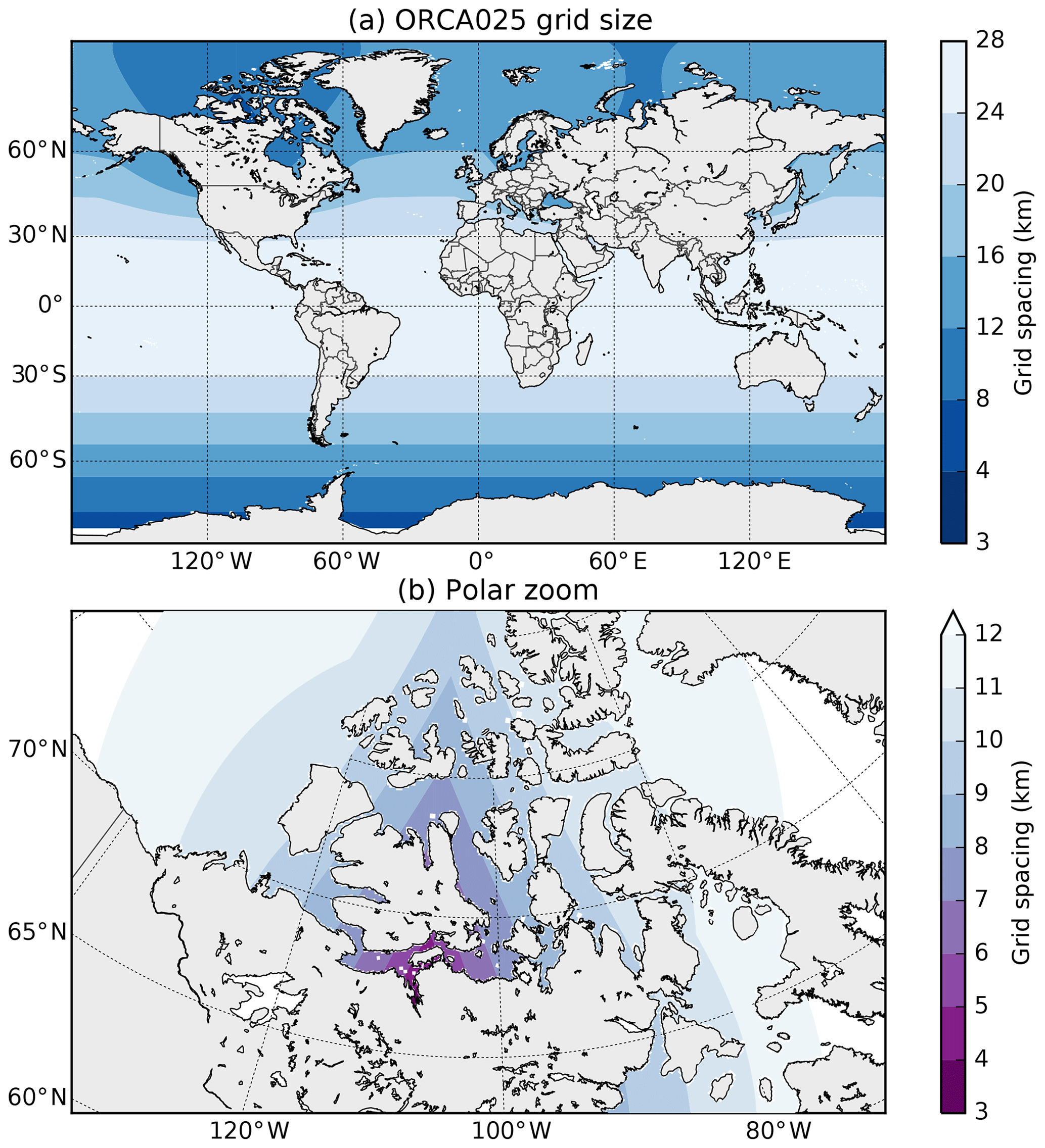
Figure 1 Grid size, defined as $min(\mathtt{e}\mathtt{1}\mathtt{t},\mathtt{e}\mathtt{2}\mathtt{t})$, on the ORCA025 grid. (a) In the global view, grid-point spacing gradually decreases from the Equator towards the north and south poles. (b) In a detail view of the north polar region, the grid is especially high resolution in the southern portion of the Canadian Arctic Archipelago, with grid-point spacing as low as 3 km.

Unfortunately, this placement causes an abundance of small grid cells in the north polar region, especially in the Canadian Arctic Archipelago. Figure 1 depicts this situation at a nominal $\mathrm{1}/\mathrm{4}{}^{\circ }$ resolution: the grid point spacing of 25–30 km near the Equator falls to 3–4 km in the archipelago. The areas in Fig. 1 with the narrowest grid spacing are also shallow seas, with depths of 200 m or less and non-tidal currents of 15–30 cm s⁻¹. This grid stretching is of particular concern when adapted to regional models such as that of Lemieux et al. (2016), which refine this grid while retaining its tripolar structure to use conforming boundary conditions.

The coordinate system is also stretched in the vertical direction. Using the z-level grid option of the NEMO-OPA model, layers near the surface are spaced much more closely together than layers nearer the ocean bottom, in order to provide adequate resolution of the mixing layer. This stretching enhances the impact of vertical advection on the vertical Courant number, even if vertical-current magnitudes are low in absolute terms; Lemarié et al. (2015) notes that vertical advection provides a tighter bound on the time step than horizontal advection.

Semi-Lagrangian advection alleviates both vertical and horizontal Courant number restrictions by tracing fluid parcels in a Lagrangian, fluid-following coordinate system. This coordinate system is defined so that the end of each time step the fluid parcels arrive on the prescribed computational grid, and the properties of the fluid parcels (in the ocean setting, temperature, salinity, and horizontal velocity) at the end of the time step (on the computational grid) are found by interpolating the previous-step, gridded values to the origin point of each parcel's trajectory. This method provides an implicit treatment of advection, allowing time steps with advective Courant numbers greater than those usually permitted by explicit, Eulerian-form models.

In this work, we describe the initial implementation of a semi-Lagrangian advection routine in NEMO-OPA, based on the configuration of Smith et al. (2018). This configuration uses a linear free surface where the vertical coordinate does not move in time, but we believe that the described method can be generalized.

1.2 Existing work

In the atmosphere, semi-Lagrangian advection is a standard technique (Robert, 1982) for the implicit treatment of advection, but especially at large scales the effects of topography are relatively gentle. In particular, trajectory calculations can proceed under the assumption that the fluid parcel does not experience strong boundary-related acceleration. In the ocean domain this assumption is strongly violated, particularly for z-level vertical grids where the bathymetry changes abruptly at lateral cell boundaries.

Some attempts have been made previously to incorporate semi-Lagrangian advection into the ocean context. The work of Casulli and Cheng (1992), which is used as part of the ELCOM lake and estuary model (Hodges and Dallimore, 2006), calculates parcel trajectories via a substepping approach, where fluid parcel trajectories are integrated via an explicit Euler method over many short steps per model time step. The two-dimensional, unstructured shallow water model of Walters et al. (2007) takes a similar approach, where it also must take at least one substep per element boundary traversed by a fluid parcel.

In this work, we overcome this difficulty with an iterative trajectory calculation which reduces in the limit to an implicit trapezoidal rule. In addition, we also derive the semi-Lagrangian advection scheme in a form which calculates effective advective tendencies, such that the advection routine can operate as a “plug-in” scheme for models which traditionally use Eulerian fluxes. We apply this to the NEMO-OPA model, and we believe this algorithm may be useful when applied to other ocean models with a structured grid.

In exchange, however, the semi-Lagrangian advection formulation departs from NEMO's finite-volume interpretation of its tracer and velocity components. By tracing infinitesimal fluid parcels, semi-Lagrangian advection treats grid-point values analogously to a finite-difference method, and as a consequence the scheme does not naturally offer conservation guarantees. This is not a primary concern for the short- to medium-term forecasting applications that form the direct target for this work, but extensions of the semi-Lagrangian scheme to ensure conservation (Lauritzen, 2007) may be needed before the technique is applicable to longer-term climate simulations.

Additionally, Leclair and Madec (2011) has developed an “arbitrary Lagrangian–Eulerian” vertical coordinate scheme, implemented in recent versions of NEMO. This scheme splits vertical motions into fast (high temporal frequency) and slow motions, and the former are treated by co-moving vertical coordinate surfaces with a regridding step. This coordinate system reduces spurious diapycnal mixing caused by the high-frequency vertical motions, and its Lagrangian treatment of these motions relaxes the corresponding stability restriction.

1.3 Organization

We first introduce the time discretization of the semi-Lagrangian scheme in Sect. 2, in order to develop a formulation that remains compatible with the common leapfrog scheme. In Sect. 3, we begin to spatially discretize the semi-Lagrangian scheme by specifying the horizontal and vertical interpolation operators, and in Sect. 4 we complete the discretization by defining the trajectory calculations. We present preliminary numerical examples in Sect. 5, demonstrating the stability of the advection scheme.

2 Time discretization

The first requirement of a semi-Lagrangian advection scheme for the NEMO-OPA model is that it be consistent with the model's overall time-stepping approach: the advection scheme is but one component of the full model.

In version 3 of NEMO-OPA, non-diffusive, non-damping processes such as advection are implemented via the leapfrog scheme (Mesinger and Arakawa, 1976), where at each time step a field f receives its new value at f^A (f “after” the time step) based on its value at the previous time step and forcing terms, which are all evaluated on the reference grid x_ref. This gives a schematic of

$$\begin{array}{}\text{(1)}& {\displaystyle }{f}^{\mathrm{A}}\left({\mathit{x}}_{\text{ref}}\right)=f^{\mathrm{B}}\left({\mathit{x}}_{\text{ref}}\right)+\mathrm{2}\mathrm{\Delta }t\mathbf{F}\left({\mathit{x}}_{\text{ref}}\right),\end{array}$$

where f^A is the field calculated at time t₀+Δt, f^B is the field evaluated at the known prior time t₀−Δt (“before”), f^N is the field at the provided time t₀ (“now”), and F is the forcing operator. The forcing operator includes advective processes at the now time level, but diffusive, damping, and hydrostatic pressure terms might be evaluated at either the before or after time levels.

This is an Eulerian approach to fluid motion, where tracer and momentum values are tracked along the fixed reference grid at all times, and fluid flows through this grid.

2.1 Semi-Lagrangian advection

In contrast, the Lagrangian advection schemes consider the fluid parcel to be the fundamental unit of discretization. In this perspective, if f is a property of a fluid parcel that is conserved along a trajectory¹, it satisfies the continuous equations:

$$\begin{array}{}\text{(2)}& {\displaystyle \frac{\mathrm{D}}{\mathrm{D}t}}f\left(\mathit{x}\right(t\left)\right)={\mathbf{F}}_L\left(\mathit{x}\right(t\left)\right),\end{array}$$

where $\frac{\mathrm{D}}{\mathrm{D}t}={\partial }_t+\mathit{u}\cdot \mathrm{\nabla }$ is the material derivative, and F_L (Lagrangian right-hand side) contains all the same forcing terms as F except those arising from tracer and momentum flux, which are included inside the material derivative.

Ordinarily, Eq. (2) is discretized so that F_L is evaluated following the Lagrangian particles in the moving coordinate frame x(t), satisfying the trajectory equation:

$$\begin{array}{}\text{(3)}& {\displaystyle \frac{\mathrm{D}}{\mathrm{D}t}}\mathit{x}\left(t\right)=\mathit{u}\left(\mathit{x}\right(t\left)\right).\end{array}$$

From an Eulerian point of view, Eq. (3) is a trivial identity based on the definition of the material derivative, but from the Lagrangian point of view, Eq. (3) must be solved to define x over time.

One technique for solving Eqs. (2) and (3) is the two-time-level implicit semi-Lagrangian method, used in the GEM atmospheric model (Girard et al., 2014), among others. Here, the F_L terms are evaluated with a trapezoidal rule, discretizing Eqs. (2) and (3) as

$$\begin{array}{}\text{(4a)}& {\displaystyle }{f}^{\mathrm{A}}\left({\mathit{x}}_{\text{ref}}\right)& {\displaystyle }=f^{\mathrm{N}}\left({\mathit{x}}^{\mathrm{D}}\right)+{\displaystyle \frac{\mathrm{\Delta }t}{\mathrm{2}}}\left({\mathbf{F}}_L^A\right({\mathit{x}}_{\text{ref}})+{\mathbf{F}}_L^N({\mathit{x}}^{\mathrm{D}}\left)\right)\text{ and}\text{(4b)}& {\displaystyle }{\mathit{x}}_{\text{ref}}& {\displaystyle }={\mathit{x}}^{\mathrm{D}}+{\displaystyle \frac{\mathrm{\Delta }t}{\mathrm{2}}}\left({\mathit{u}}^A\right({\mathit{x}}_{\text{ref}})+{\mathit{u}}^N({\mathit{x}}^{\mathrm{D}}\left)\right).\end{array}$$

The trajectory Eq. (4b) acts to implicitly define the paths of the traced fluid parcels, where each location on x_ref is associated with a corresponding departure-point location x^D. Over the single time step, fluid parcels depart from x^D (which in general is not aligned with the grid) and arrive on the reference grid.

This off-grid, departure point evaluation of u and F_L is fundamental to Lagrangian and semi-Lagrangian methods, and f^N(x^D) (${\mathbf{F}}_L^N\left({\mathit{x}}^{\mathrm{D}}\right)$) can be written more simply as f^D (${\mathbf{F}}_L^{\mathrm{D}}$) for “departure-point f (F)”. Neither the time-implicit evaluations (generally) nor the off-grid evaluations (of non-advective forcing) are compatible with the core structure of NEMO-OPA, which considers advection to be just one of many independent operators influencing the F term of Eq. (1).

2.2 Reconciliation

Implementing semi-Lagrangian advection in NEMO-OPA requires adopting as much of the framework of Eq. (1) as possible, without changing the evaluation of non-advective forcing terms. Effectively, the semi-Lagrangian advection routine must ultimately supply a time trend that, from the perspective of the leapfrog time-step algorithm, is indistinguishable from a conventional flux-form advection operator.

To effect this, consider Eq. (2) without forcing terms (F_L=0). The function f is preserved following the flow, so this gives the simply written

$$\begin{array}{}\text{(5)}& f^{\mathrm{A}}=f^{\mathrm{D}}.\end{array}$$

This is approximated by taking one time step of Eq. (1) (with only advective forcing F_adv), but the latter involves integrating over the whole interval from t₀−Δt to t₀+Δt. Thus, we should identify f^D (and the departure points generally) not with the now time level in the leapfrog scheme but rather with the before time level. Doing so and equating Eqs. (5) and (1) gives

$$\begin{array}{}\text{(6)}& {\displaystyle }{f}^{\mathrm{A}}& {\displaystyle }=f^{\mathrm{B}}+\mathrm{2}\mathrm{\Delta }t{\mathbf{F}}_{\text{adv}}=f^{\mathrm{B}}\left({\mathit{x}}^{\mathrm{D}}\right)\text{, or}\text{(7)}& {\displaystyle }{\mathbf{F}}_{\text{adv}}& {\displaystyle }={\displaystyle \frac{\mathrm{1}}{\mathrm{2}\mathrm{\Delta }t}}(f^{\mathrm{B}}-f^{\mathrm{B}}({\mathit{x}}^{\mathrm{D}}\left)\right).\end{array}$$

Equation (7) is prescriptive, and it gives the necessary trend for the leapfrog algorithm. Evaluating it requires f only at the already known, before time level and calculation of the departure points x^D. This calculation is further simplified by basing the departure points on the time-centered velocities u^N, and the exact algorithm for this calculation will be discussed in more detail in Sect. 4.

2.3 Effects of the Asselin filter

To prevent decoupling of odd and even time steps (damping the computational mode), NEMO-OPA is typically configured to use the Asselin time filter (Asselin, 1972), which adds a small time damping proportional to $\frac{{\partial }^{\mathrm{2}}}{\partial t^{\mathrm{2}}}f$. Using the notation of Shchepetkin and McWilliams (2005) adapted to Eq. (1), the filter extends the time-marching scheme to the sequence:

$$\begin{array}{}\text{(8a)}& {\displaystyle }{f}^{\mathrm{A}*}& {\displaystyle }\leftarrow f^{\mathrm{B}}+\mathrm{2}\mathrm{\Delta }t{\mathbf{F}}^{\mathrm{N}*}\text{(8b)}& {\displaystyle }{f}^{\mathrm{N}}& {\displaystyle }\leftarrow \mathit{ϵ}{f}^{\mathrm{A}*}+(\mathrm{1}-\mathrm{2}\mathit{ϵ})f^{\mathrm{N}*}+\mathit{ϵ}{f}^{\mathrm{B}}\text{(8c)}& {\displaystyle }{f}^{\mathrm{N}*}& {\displaystyle }\leftarrow f^{\mathrm{A}*}\text{(8d)}& {\displaystyle }{f}^{\mathrm{B}}& {\displaystyle }\leftarrow f^{\mathrm{N}}.\end{array}$$

Equation (8a) is the direct equivalent of Eq. (1), creating a provisional after value f^A*. Equation (8b) applies the filter (with a strength parameter ϵ) with this value and the previous step's provisional field to define a final now field, and finally Eqs. (8c) and (8d) are “bookkeeping” steps to shift field labels to become ready for the next time step. The forcing operator F^N* is evaluated based on the provisionally defined fields.

In applying this filter with the semi-Lagrangian forcing, Eq. (7) is oblivious to the presence of the filter or the difference between f^N and f^N*. Substituting Eq. (7) into Eq. (8a) and applying Eqs. (8c) and (8d) to Eqs. (8a) and (8b) gives the update equation:

$$\begin{array}{}\text{(9)}& \left(\begin{array}{c}{f}^{\mathrm{N}*}\\ f^{\mathrm{B}}\end{array}\right)\leftarrow \left(\begin{array}{c}{f}^{\mathrm{B}}\left({\mathit{x}}^{\mathrm{D}}\right)\\ \mathit{ϵ}\left(f^{\mathrm{B}}\right({\mathit{x}}^{\mathrm{D}})+f^{\mathrm{B}}({\mathit{x}}_{\text{ref}}\left)\right)+(\mathrm{1}-\mathrm{2}\mathit{ϵ})f^{\mathrm{N}*}\left({\mathit{x}}_{\text{ref}}\right)\end{array}\right).\end{array}$$

In the case of one-dimensional advection by a constant velocity u₀, the trajectory calculation is trivial, and

$$\begin{array}{}\text{(10)}& {\mathit{x}}^{\mathrm{D}}=x^{\mathrm{D}}=x_{\text{ref}}-\mathrm{2}\mathrm{\Delta }t{u}_{\mathrm{0}}.\end{array}$$

Since Eq. (9) is linear, we can also take its Fourier decomposition in space and consider only a single, arbitrary wave mode, giving $f=\widehat{f}\left(t\right)\exp \mathbf{i}kx$ for a time-varying coefficient $\widehat{f}$. Applying this to Eq. (9) casts the update in a matrix form as

$$\begin{array}{}\text{(11)}& \left(\begin{array}{c}{\widehat{f}}^{\mathrm{N}*}\\ {\widehat{f}}^B\end{array}\right)\leftarrow \left(\begin{array}{cc}\mathrm{0}& \exp (-\mathrm{2}\mathbf{i}k{u}_{\mathrm{0}}\mathrm{\Delta }t)\\ \mathrm{1}-\mathrm{2}\mathit{ϵ}& \mathit{ϵ}(\mathrm{1}+\exp (-\mathrm{2}\mathbf{i}k{u}_{\mathrm{0}}\mathrm{\Delta }t\left)\right)\end{array}\right)\left(\begin{array}{c}{\widehat{f}}^{\mathrm{N}*}\\ {\widehat{f}}^B\end{array}\right).\end{array}$$

The time stability of this filter is then governed by the eigenvalues of this matrix. Using the shorthand $\mathit{\omega }=-k{u}_{\mathrm{0}}\mathrm{\Delta }t$, these eigenvalues are

$$\begin{array}{ll}{\displaystyle }& {\displaystyle }{\mathit{\lambda }}_{\mathrm{1},\mathrm{2}}=\\ \text{(12)}& {\displaystyle }& {\displaystyle }{\displaystyle \frac{\mathrm{1}}{\mathrm{2}}}\left(\mathit{ϵ}\right(\mathrm{1}+e^{\left(\mathrm{2}\mathbf{i}\mathit{\omega }\right)})\pm \sqrt{{\mathit{ϵ}}^{\mathrm{2}}(\mathrm{1}+e^{\left(\mathrm{2}\mathbf{i}\mathit{\omega }\right)}{)}^{\mathrm{2}}+(\mathrm{4}-\mathrm{8}\mathit{ϵ})e^{\left(\mathrm{2}\mathbf{i}\mathit{\omega }\right)}}),\end{array}$$

and to leading order in ϵ, these eigenvalues have squared magnitudes of

$$\begin{array}{}\text{(13)}& |{\mathit{\lambda }}_{\mathrm{1},\mathrm{2}}{|}^{\mathrm{2}}=\mathrm{1}-\mathrm{2}\mathit{ϵ}\pm \mathrm{2}\mathit{ϵ}\cos (\mathit{\omega })+O({\mathit{ϵ}}^{\mathrm{2}}),\end{array}$$

signifying stability ($\left|\mathit{\lambda }\right|\le \mathrm{1}$) for all values of ω and thus all Courant numbers.

3 Interpolation

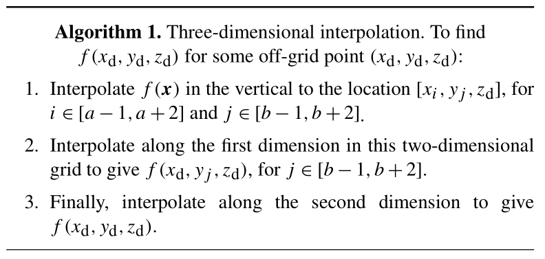
To perform the off-grid interpolations in Eq. (7) to find f^B(x^D), this method fits a cubic polynomial to the underlying function. If the single departure point ${\mathit{x}}_{\mathrm{d}}=(x_{\mathrm{d}},y_{\mathrm{d}},z_{\mathrm{d}})$ lies within² $(x_a,x_{a+\mathrm{1}})\times (y_b,y_{b+\mathrm{1}})\times (z_c,z_{c+\mathrm{1}})$ for integer values of a, b, and c coinciding with grid-point locations, the full interpolation stencil consists of the grid-index cube $i\in [a-\mathrm{1},a+\mathrm{2}]$, $j\in [b-\mathrm{1},b+\mathrm{2}]$, and $k\in [c-\mathrm{1},c+\mathrm{2}]$.

This grid cube contains up to 64 grid points where f(x) might be defined (subject to boundary conditions), and building a complete interpolation stencil would be cumbersome and inefficient. Instead, the interpolation procedure takes advantage of the tensor-product nature of the grid to separate interpolation along each dimension:

To effect the one-dimensional interpolations in Algorithm 1, we make use of the cubic Hermite polynomials (Hildebrand, 1974). On the interval $\mathrm{0}\le \mathit{\chi }\le \mathrm{1}$, these polynomials are

$$\begin{array}{}\text{(14)}& {\displaystyle }\begin{array}{rl}{\displaystyle }{h}_{\mathrm{00}}\left(\mathit{\chi }\right)& {\displaystyle }=\mathrm{2}{\mathit{\chi }}^{\mathrm{3}}-\mathrm{3}{\mathit{\chi }}^{\mathrm{2}}+\mathrm{1},\\ {\displaystyle }{h}_{\mathrm{01}}\left(\mathit{\chi }\right)& {\displaystyle }=-\mathrm{2}{\mathit{\chi }}^{\mathrm{3}}+\mathrm{3}{\mathit{\chi }}^{\mathrm{2}},\\ {\displaystyle }{h}_{\mathrm{10}}\left(\mathit{\chi }\right)& {\displaystyle }={\mathit{\chi }}^{\mathrm{3}}-\mathrm{2}{\mathit{\chi }}^{\mathrm{2}}+\mathit{\chi }\text{, and}\\ {\displaystyle }{h}_{\mathrm{01}}\left(\mathit{\chi }\right)& {\displaystyle }={\mathit{\chi }}^{\mathrm{3}}-{\mathit{\chi }}^{\mathrm{2}},\end{array}\end{array}$$

and a function f(χ) defined on this interval is interpolated via

$$\begin{array}{ll}{\displaystyle }f\left(\mathit{\chi }\right)\approx & {\displaystyle }f\left(\mathrm{0}\right)h_{\mathrm{00}}\left(\mathit{\chi }\right)+f^{\prime }\left(\mathrm{0}\right)h_{\mathrm{10}}\left(\mathit{\chi }\right)+f\left(\mathrm{1}\right)h_{\mathrm{01}}\left(\mathit{\chi }\right)\\ \text{(15)}& {\displaystyle }& {\displaystyle }+f^{\prime }\left(\mathrm{1}\right)h_{\mathrm{11}}\left(\mathit{\chi }\right).\end{array}$$

Here, we prefer to use the cubic Hermite polynomials over simple Lagrange polynomial interpolation because the former choice allows greater freedom (via Eq. 15) in implementation. If f^′ is approximated by a four-point finite-difference stencil, then Eq. (15) reduces to Lagrange interpolation. However, we can also make other choices for f^′ to impose desirable properties: restricting f^′ to have the same sign as the discrete difference imposes a type of slope limiting, and calculating f^′ through a three-point stencil provides for continuous derivatives. These approaches are discussed in more detail in the following sections.

Interpolation using the above algorithm involves appropriately defining the interval to be scaled to [0,1] and approximating f^′ at the endpoints. Because of the high aspect ratio of oceanic flows and the special character of vertical motion in a stratified ocean, these approximations differ between the horizontal and vertical interpolations.

3.1 Horizontal interpolation

In the horizontal, the interpolation in Eq. (15) can be directly conducted in grid-index space. Even when the underlying grid is mapped to the sphere, such as in the ORCA global grid (Madec, 2008, chap. 16), the grid generally transitions smoothly and slowly from point to point³. The physical trajectory departure location x_d (and y_d) can be translated into a fractional grid index offset by dividing by the appropriate grid scale factor, available inside the NEMO-OPA source code as one of e[12][tuv].

Achieving third-order accuracy inside Eq. (15) is possible, but doing so requires an equally accurate estimate for f^′. Unfortunately, interpolating successively in one dimension using the above algorithm does not allow for precomputation of these derivatives: after the vertical interpolation step, all of the function values need to be taken off grid, so any precomputed derivatives would themselves require interpolation. Instead, sufficiently accurate estimates of the derivative are available by applying a finite-difference formula to the function values themselves.

3.1.1 Derivative estimates

For notational simplicity, begin with the last step of the above algorithm where we have $f(x_{\mathrm{d}},y_j,z_{\mathrm{d}})$ and would like to estimate $f(x_{\mathrm{d}},y_{\mathrm{d}},z_{\mathrm{d}})$. If y_d lies between y₀ and y₁, then the four-point interpolation stencil implies that we have computed $f(x_{\mathrm{d}},y_j,z_{\mathrm{d}})$ for $j=-\mathrm{1},\mathrm{0},\mathrm{1},\mathrm{2}$. To emphasize that this is now a one-dimensional interpolation problem, let $g\left(j\right)=f(x_{\mathrm{d}},y_j,z_{\mathrm{d}})$, such that $f(x_{\mathrm{d}},y_{\mathrm{d}},z_{\mathrm{d}})=g\left(j^{\prime }\right)$ for some $j^{\prime }\in [\mathrm{0},\mathrm{1}]$. In this domain, g^′(0) and g^′(1) can be approximated by the finite differences:

$$\begin{array}{}\text{(16a)}& {\displaystyle }{g}^{\prime }\left(\mathrm{0}\right)& {\displaystyle }\approx -{\displaystyle \frac{\mathrm{1}}{\mathrm{3}}}g(-\mathrm{1})-{\displaystyle \frac{\mathrm{1}}{\mathrm{2}}}g\left(\mathrm{0}\right)+g\left(\mathrm{1}\right)-{\displaystyle \frac{\mathrm{1}}{\mathrm{6}}}g\left(\mathrm{2}\right)\text{ and }\text{(16b)}& {\displaystyle }{g}^{\prime }\left(\mathrm{1}\right)& {\displaystyle }\approx {\displaystyle \frac{\mathrm{1}}{\mathrm{6}}}g(-\mathrm{1})-g\left(\mathrm{0}\right)+{\displaystyle \frac{\mathrm{1}}{\mathrm{2}}}g\left(\mathrm{1}\right)+{\displaystyle \frac{\mathrm{1}}{\mathrm{3}}}g\left(\mathrm{2}\right),\end{array}$$

which then substitute for the appropriate derivatives in Eq. (15).

These finite differences are exact expressions for the first derivative for polynomials up to third order in j, and their use essentially converts Eq. (15) to interpolation via Lagrange polynomials. The Hermite polynomial form, however, allows for an easier imposition of boundary conditions.

3.1.2 Boundary conditions

On the NEMO-OPA z-level grid, the lateral boundaries coincide with u and v points (velocity points), which are spaced halfway between t points (tracer points). Tracer points that lie inside the land region are masked (𝚝𝚖𝚊𝚜𝚔=0) as are velocity points that are at the edge of or within the masked region. This arrangement is illustrated for a sample region in Fig. 2.

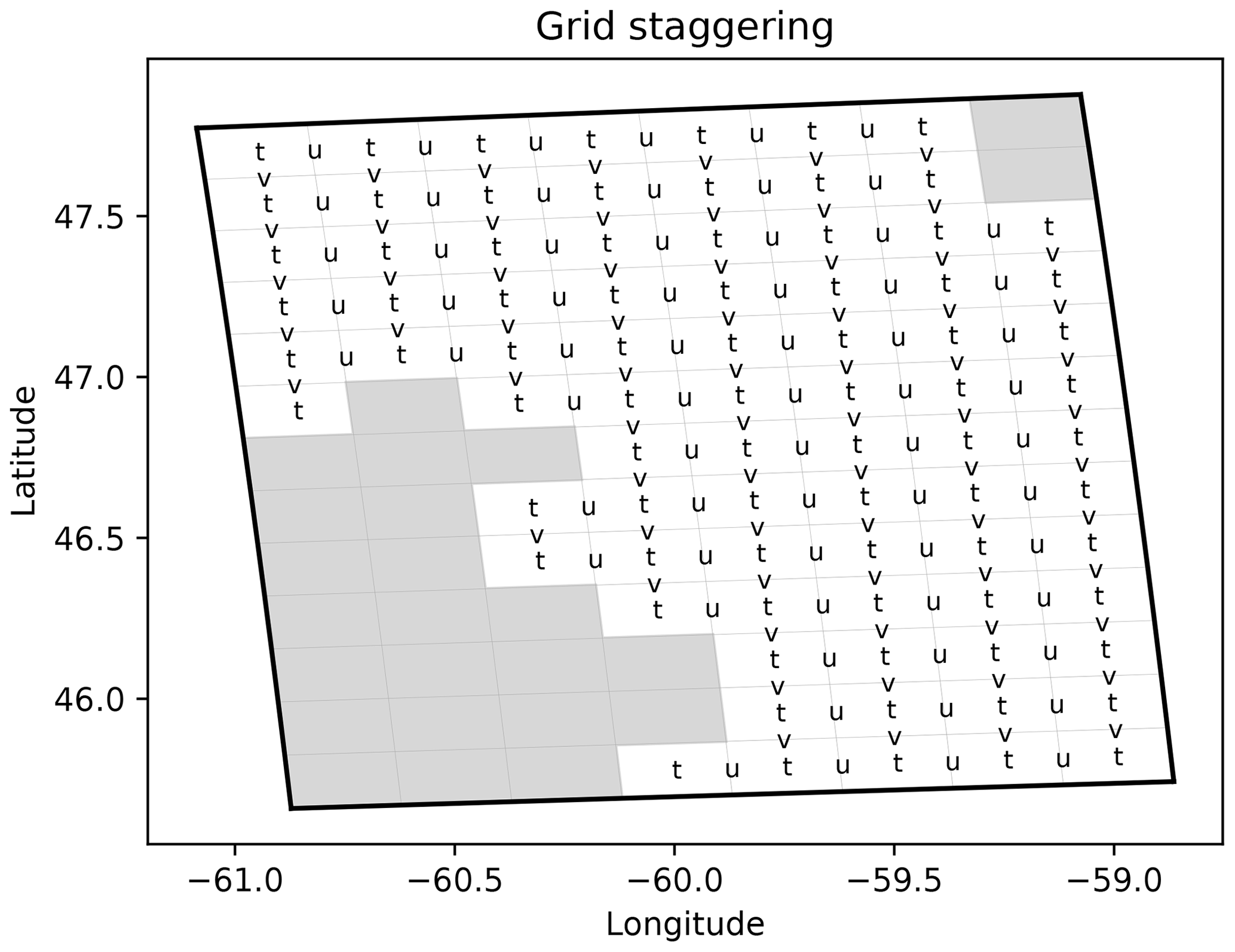
Figure 2 Grid point locations (letters) and land region (grey region) for a sample horizontal plane in the Gulf of Saint Lawrence, between Nova Scotia and New Brunswick. The horizontal velocities (u and v) are staggered with respect to temperature and salinity (t), and the edge of the land area is coincident with the lines between velocity-point locations.

The physical interpretation of the boundary varies with respect to the field being interpolated. For tracers, lateral boundaries imply no-flux conditions for the purposes of advection, which in turn implies a zero derivative at the boundary. The normal velocity (u with respect to a boundary along the first grid dimension, v with respect to a grid boundary along the second) is obviously constrained to zero by geometry to give a Dirichlet boundary condition, whereas the tangential velocity can be set as free-slip, no-slip, or some combination via a namelist entry. In the subsequent, we assume that velocity has a free-slip boundary condition, with boundary friction left for future work.

If a boundary occurs in the left portion of the interpolation stencil, there are a total of seven cases (see Algorithm 2).

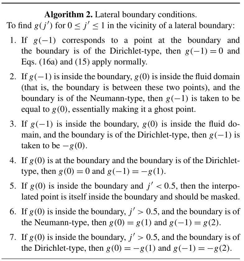
For boundaries that occur in the right portion of the interpolation stencil, the values taken for ghost points are given symmetrically.

The combination of “the grid point is at the boundary” and “the boundary is of Neumann-type” is missing from Algorithm 2. This construction is forbidden by the grid structure of NEMO-OPA, where tangential velocity is located one half-cell away from a boundary.

For two-dimensional interpolation, Algorithm 2 applies independently to each dimension. When interpolating along x, the points $f(x_{\mathrm{d}},y_j,z_{\mathrm{d}})$ will each individually be either in the ocean domain and valid or in the land domain and masked, which provides the values necessary to compute $f(x_{\mathrm{d}},y_{\mathrm{d}},z_{\mathrm{d}})$. This off-grid point itself must lie in water, which imposes a strong requirement on the trajectory calculations to be discussed in Sect. 4.

3.1.3 Slope limiting

As a final step, once values for the function and its derivative at the interval endpoints are specified, the derivative values are limited to help prevent new maxima in the interpolated function. In particular, if g(0) is a local minimum (maximum) among itself, g(−1), and g(1), then g^′(0) is set to zero if the above procedure finds that it would be negative (positive). A similar procedure applies symmetrically for g^′(1) if g(1) is a relative extremum.

This limiting is milder than methods derived from Bermejo and Staniforth (1992), which would strictly preserve positivity for any j^′, but it effectively limits excursions when j^′ is close to 0 or 1. Without such limiting, numerical testing showed that semi-Lagrangian advection of temperature and salinity could cause weak instabilities near the coastline, where a locally extreme temperature or salinity could become “trapped” near the coast and slowly amplified.

3.2 Vertical interpolation

Vertical motion in the NEMO-OPA model differs from horizontal motion in a number of respects:

• Vertical gradients of temperature and density are much stronger than typical horizontal gradients, especially near the surface.

• Typical vertical grids used with NEMO-OPA are strongly stretched, with a higher resolution near the surface and a lower resolution in the deep ocean.

• Vertical flow is often oscillatory, where vertical motion is driven by barotropic and baroclinic waves.

The horizontal interpolation described in Sect. 3.1 is third-order accurate; with the provided one-sided formulas for calculating the endpoint derivatives it reduces to a four-point (cubic) Lagrangian interpolation process. However, the smooth field implied by this interpolation process is only C⁰ continuous: f(x_j−ϵ) “sees” $f_j^{\prime }$ calculated from f(x_j−2) to f(x_j+1), whereas f(x_j+ϵ) sees $f_j^{\prime }$ from f(x_j−1) to f(x_j+2).

We do not find this to be a practical concern for horizontal interpolation, since horizontal currents in most of the ocean tend to be dominated by relatively steady quasi-geostrophic motions. In the vertical, however, we found that even low-amplitude oscillations caused by high-frequency gravity waves would cause the temperature and salinity fields to drift. The mechanism is that a fluid parcel displaced upwards by ϵ in one time step and downwards by ϵ in the next time step would see an effective diffusion proportional to the jump between the upward- and downward-looking vertical derivatives.

To maintain global accuracy, we impose C¹ continuity in the vertical direction through an alternative treatment of the vertical derivative. Instead of applying Eqs. (16), we treat the physical depth (rather than grid index) as the relevant coordinate and construct a centered estimate of the derivative.

For a function f(z_n) defined at the z_n levels, define $\mathrm{\Delta }{f}^{+}=f\left(z_{n+\mathrm{1}}\right)-f\left(z_n\right)$, $\mathrm{\Delta }{f}^{-}=f\left(z_n\right)-f\left(z_{n-\mathrm{1}}\right)$, $\mathrm{\Delta }{z}^{+}=z_{n+\mathrm{1}}-z_n$, and $\mathrm{\Delta }{z}^{-}=z_n-z_{n-\mathrm{1}}$. These differences combine to give the estimated derivative:

$$\begin{array}{}\text{(17)}& f_z\left(z_n\right)\approx {\displaystyle \frac{\mathrm{1}}{\mathrm{\Delta }{z}^{-}+\mathrm{\Delta }{z}^{+}}}({\displaystyle \frac{\mathrm{\Delta }{z}^{-}}{\mathrm{\Delta }{z}^{+}}}\mathrm{\Delta }{f}^{+}+{\displaystyle \frac{\mathrm{\Delta }{z}^{+}}{\mathrm{\Delta }{z}^{-}}}\mathrm{\Delta }{f}^{-}),\end{array}$$

which is accurate to O(Δz²) for the derivative and accurately reproduces quadratic functions of z. In the limiting case of a constant Δz (equispaced vertical levels), this formula reduces to the classic centered difference.

Because vertical interpolation comes first in Algorithm 1, Eq. (17) need be evaluated only at grid points, and in fact it may be precomputed for the entire grid for a given function and time step. This is a key advantage of placing vertical interpolation first in the interpolation sequence, and it avoids duplication of work.

Whereas interpolation near the horizontal boundaries is complicated by the many combinations of grid staggering and physical boundary conditions, interpolation near the vertical boundaries is much simpler. On the NEMO grid, tracers and horizontal velocities lie along the same vertical level, and these levels are staggered one half-cell away from the boundaries. Likewise, the natural vertical boundary condition for both tracer and horizontal velocity fields is a no-flux boundary condition; NEMO-OPA models boundary-layer friction in another module. Interpolation near the boundaries then proceeds in two steps.

The first step is to define f_z at the top and bottom points in the water column, for which the central difference formula of Eq. (17) is not directly valid. Here, we approximate the physical no-flux condition through a fictitious ghost point such that $\mathrm{\Delta }{f}^{-}=\mathrm{0}$ at the top boundary and $\mathrm{\Delta }{f}^{+}=\mathrm{0}$ at the bottom boundary, with the respective Δz matching the layer thickness (e3t).

The second step is to define how Eq. (15) applies to the interval between the grid level and the physical boundary. Here, the no-flux boundary conditions reduce to even symmetry, and the derivative at the ghost points is the negative of the vertical derivative calculated for the in-boundary point. Near the free surface, if the interpolation point is above the level of the free surface (above z=0), then it is clamped to the surface itself. Near the ocean bottom, if the interpolation point is below the level of the ocean bottom (below $z=z_{max}$) then the point is masked and is treated as an “inside the boundary” point for the purposes of horizontal interpolation above.

3.2.1 Treatment of partial cells

Over most of the domain, this interpolation works well. Although there is no guarantee of positivity in the derivative formulation of Eq. (17), overshoots and the consequent generation of spurious maxima are limited. For the tests presented in Sect. 5, there was no need for slope limiting for vertical interpolation over most of the domain.

One exception to this rule is at the bottom boundary. Here, vertical levels are spaced far apart, but to better represent the ocean bottom the z-level grid of NEMO-OPA uses a partial cell configuration (Madec, 2008, sec. 5.9). For water columns where the bottom-most cell is much deeper than its neighbours, a local (small) upwelling can cause an overshoot of temperature or salinity that spuriously increases the local density but does not diminish the upwelling. Over time, the maxima-increasing trend can accumulate and cause some points at the bottom boundary to reach implausibly cold temperatures (below $-\mathrm{10}{}^{\circ }\mathrm{C}$, for example) or high salinities. In the absence of explicit horizontal diffusion (which would mix this maximum into more dynamically active regions), these spurious maxima do not generally corrupt the flow, although they obviously would corrupt whole-ocean (or whole-level) statistics such as average or extreme temperatures.

Near these boundary cells, vertical limiting is implemented in the simplest possible way: the interpolation of Eq. (15) is replaced with a constant, such that f(z)=f(z_k) over the interval from z_k downwards to the physical boundary.

Implementing this limiting over the whole bottom level is possible, but that is far stronger than necessary and leads to erroneous diffusion along gentle slopes. When the bottom layer is composed of partial cells of varying thickness, even interpolation along a horizontal plane (that is, without changing physical depth) requires vertical interpolation in grid space to find that constant level in adjoining columns. Imposing vertical limiting along the whole bottom level effects undesired horizontal diffusion, even though the problem solved by limiting is observed when adjoining cells have large relative thickness variations.

As a compromise between these two errors, we only apply the described limiting to vertical interpolation for cells at the bottom boundary which have a layer thickness greater than 1.75 times that of their “thinnest” neighbour.

This exact threshold is empirical, and other grids might require a retuning of this parameter. Ideally, the grid generation itself would avoid abrupt transitions in cell-layer thicknesses, but adding such a restriction would make this advection scheme useless as a drop-in replacement for the standard advection routines of NEMO-OPA.

3.3 A numerical example

As a simple numerical example, consider the case of a tracer being advected in a rectangular, two-dimensional domain by an internal wave and a background current. This tracer satisfies the advection equation

$$\begin{array}{}\text{(18)}& {\displaystyle \frac{\partial \mathit{\sigma }}{\partial t}}-u(x,z,t){\displaystyle \frac{\partial \mathit{\sigma }}{\partial x}}-w(x,z,t){\displaystyle \frac{\partial \mathit{\sigma }}{\partial z}}=\mathrm{0}\end{array}$$

for some prescribed velocity field (u,w).

If this tracer field $\mathit{\sigma }(x,z,t)$ would be a function of z alone, i.e. $\overline{\mathit{\sigma }}\left(z\right)$, if not for the wave motion, then its motion is analytically given by

$$\begin{array}{}\text{(19)}& \mathit{\sigma }(x,z,t)=\overline{\mathit{\sigma }}(z-\mathit{\eta }(x-(c+u_{\mathrm{0}})t,z\left)\right),\end{array}$$

where η(x,z) is the isopycnal displacement, u₀ is the x-directed background current (uniform in z), and c is the phase speed of the wave. Following Turkington et al. (1991), a streamfunction defined as

$$\begin{array}{}\text{(20)}& \mathit{\psi }(x,z,t)=c\mathit{\eta }(x,z,t)-u_{\mathrm{0}}z\end{array}$$

gives velocities

$$\begin{array}{}\text{(21a)}& {\displaystyle }u& {\displaystyle }=-{\mathit{\psi }}_z\text{(21b)}& {\displaystyle }w& {\displaystyle }={\mathit{\psi }}_x,\end{array}$$

which are exact solutions of Eq. (18) for $\mathit{\sigma }(x,z,t)$.

To give an internal wave that respects no-flux conditions at the top and bottom of the domain, we set

$$\begin{array}{}\text{(22)}& \mathit{\eta }(x,z,t)=A\cos \left(k\right(x-(c+u_{\mathrm{0}})t\left)\right)\sin \left(mz\right),\end{array}$$

where k and m are horizontal and vertical wavenumbers respectively, and A is the wave amplitude. For a domain of size L_x in the horizontal (periodic) and L_z in the vertical, $k=\mathrm{2}\mathit{\pi }/L_x$ and $m=\mathit{\pi }/L_z$ give the lowest internal wave mode, used here.

In dimensional units, we take the model domain to be a channel L_x=1 km long and L_z=100 m deep with a background current of $u_{\mathrm{0}}=\mathrm{1}\mathrm{m}{\mathrm{s}}^{-\mathrm{1}}$, and we set $c=N/\sqrt{k^{\mathrm{2}}+m^{\mathrm{2}}}$ based on a mean buoyancy frequency of $N=\mathrm{0.03}{\mathrm{s}}^{-\mathrm{1}}$, which corresponds to a 1 % density change from the surface to the bottom of the channel. With a wave amplitude of A=10 m, the maximum wave-induced current is about 10 % of u₀, and the phase speed is $c\approx \mathrm{0.94}\mathrm{m}{\mathrm{s}}^{-\mathrm{1}}$.

In order to represent the pycnocline found in many ocean waters, we choose⁴ $\overline{\mathit{\sigma }}\left(z\right)=\tanh (\frac{\mathrm{1}}{\mathrm{2}}-\frac{\mathrm{1}}{\mathrm{10}}z{L}_y^{-\mathrm{1}})$. The domain is discretized by N_x×N_y points, defined as

$$\begin{array}{}\text{(23a)}& {\displaystyle }{x}_i& {\displaystyle }=-{\displaystyle \frac{L_x}{\mathrm{2}}}+L_x{\displaystyle \frac{i-\mathrm{0.5}}{N_x}}\text{ and}\text{(23b)}& {\displaystyle }{z}_j& {\displaystyle }={\displaystyle \frac{L_z}{\mathrm{2}}}(\mathrm{1}+{\displaystyle \frac{{\mathit{\alpha }}_j+{\mathit{\alpha }}_j^{\mathrm{3}}}{\mathrm{2}}}),\end{array}$$

where $i=\mathrm{1},\mathrm{2},\mathrm{\cdots },N_x$, $j=\mathrm{1},\mathrm{2},\mathrm{\cdots },N_z$, and

$$\begin{array}{}\text{(23c)}& {\mathit{\alpha }}_j=\mathrm{2}{\displaystyle \frac{j-\mathrm{0.5}}{N_z}}-\mathrm{1}.\end{array}$$

This implements a stretched vertical coordinate that increases the vertical resolution in the vicinity of the pycnocline.

3.3.1 Semi-Lagrangian advection

In integrating this system with semi-Lagrangian advection, the leapfrog method reduces to an Euler method of twice the time step because there is no external forcing. The time-discrete equation is

$$\begin{array}{}\text{(24)}& \mathit{\sigma }(x_i,z_j,t+\mathrm{2}\mathrm{\Delta }t)=\mathit{\sigma }(x_{\mathrm{d}\left(ij\right)},z_{\mathrm{d}\left(ij\right)},t),\end{array}$$

where (x_d(ij),z_d(ij)) is the departure point of the trajectory that arrives at the grid point (x_i,z_j), and the off-grid evaluation of σ proceeds via the interpolation processes described earlier without slope limiting.

The departure points are given by the trapezoidal rule⁵ with a time-centered evaluation of velocity:

$$\begin{array}{ll}{\displaystyle }{x}_i-x_{\mathrm{d}\left(ij\right)}=& {\displaystyle }\mathrm{\Delta }t\left(u\right(x_i,z_j,t+\mathrm{\Delta }t)\\ \text{(25a)}& {\displaystyle }& {\displaystyle }+u(x_{\mathrm{d}\left(ij\right)},z_{\mathrm{d}\left(ij\right)},t+\mathrm{\Delta }t)){\displaystyle }{z}_j-z_{\mathrm{d}\left(ij\right)}=& {\displaystyle }\mathrm{\Delta }t\left(w\right(x_i,z_j,t+\mathrm{\Delta }t)\\ \text{(25b)}& {\displaystyle }& {\displaystyle }+w(x_{\mathrm{d}\left(ij\right)},z_{\mathrm{d}\left(ij\right)},t+\mathrm{\Delta }t)),\end{array}$$

where the velocities are evaluated exactly via Eq. (21). The overall system Eq. (25) is solved via simple iteration, with an initial guess given by setting $(x,z{)}_{\mathrm{d}\left(ij\right)}=(x,z{)}_{ij}$.

This algorithm is stable for large time steps, so we tested this system for time steps corresponding to Courant numbers of 0.2 and 2.1, with spatial grid resolutions between 40×4 and 2560×256. The final integration time was chosen to be $t_{\text{fin}}=\mathrm{5}{L}_x/u_{\mathrm{0}}$, which allowed the wave to propagate through the domain several times. Since the exact solution is analytically known, we recorded the maximum error experienced over the integration, and error convergence rates are shown in Fig. 3.

3.3.2 Flux-form advection

As a control, we also integrate this system in flux form, i.e. ${\mathit{\sigma }}_t-\mathrm{\nabla }\cdot \left(\mathit{u}\mathit{\sigma }\right)=\mathrm{0}$, via centered differences, with σ evaluated at the midpoints between grid cells via a simple average, matching the central difference tracer advection scheme in NEMO-OPA.

The velocity field given by Eq. (20) is divergence free, so this form of the equation is pointwise equivalent to Eq. (18). However, this no longer holds after discretization. In order to eliminate the divergence error, the velocity field is defined by creating the streamfunction at the staggered points $(x_{i+\mathrm{1}/\mathrm{2}},z_{j+\mathrm{1}/\mathrm{2}})$ and defining discrete velocities u and w via the discrete equivalents to Eq. (21). With this modification, the discrete flux-form operator is equivalent to a discrete advection equation.

After leapfrog discretization in time, the discretized equation is

$$\begin{array}{}\text{(26)}& {\displaystyle }\begin{array}{rl}{\displaystyle }& {\displaystyle }\mathit{\sigma }(x_i,z_j,t+\mathrm{\Delta }t)=\mathit{\sigma }(x_i,z_j,t-\mathrm{\Delta }t)\\ {\displaystyle }& {\displaystyle }+\mathrm{2}{\displaystyle \frac{\mathrm{\Delta }t}{\mathrm{\Delta }x\mathrm{\Delta }{z}_j}}\left({\displaystyle \frac{\mathrm{\Delta }{z}_j}{\mathrm{2}}}\right(u(x_{i-\mathrm{1}/\mathrm{2}},z_j,t)\left(\mathit{\sigma }\right(x_{i-\mathrm{1}},z_j,t)\\ {\displaystyle }& {\displaystyle }+\mathit{\sigma }(x_i,z_j,t))\\ {\displaystyle }& {\displaystyle }-u(x_{i+\mathrm{1}/\mathrm{2}},z_j,t)\left(\mathit{\sigma }\right(x_i,z_j,t)+\mathit{\sigma }(x_{i+\mathrm{1}},z_j,t\left)\right))\\ {\displaystyle }& {\displaystyle }+{\displaystyle \frac{\mathrm{\Delta }x}{\mathrm{2}}}\left(w\right(x_i,z_{j-\mathrm{1}/\mathrm{2}},t\left)\right(\mathit{\sigma }(x_i,z_{j-\mathrm{1}},t)+\mathit{\sigma }(x_i,z_j,t))\\ {\displaystyle }& {\displaystyle }-w(x_i,z_{j+\mathrm{1}/\mathrm{2}},t)\left(\mathit{\sigma }\right(x_i,z_j,t)+\mathit{\sigma }(x_i,z_{j+\mathrm{1}},t\left)\right)\left)\right),\end{array}\end{array}$$

where $\mathrm{\Delta }{z}_j=z_{j+\mathrm{1}/\mathrm{2}}-z_{j-\mathrm{1}/\mathrm{2}}=\frac{\mathrm{1}}{\mathrm{2}}(z_{j+\mathrm{1}}-z_{j-\mathrm{1}})$. For the first time step, a single Euler step is taken of size Δt with time-centered velocities ($t=\mathrm{\Delta }t/\mathrm{2}$).

As usual, this leapfrog time-stepping algorithm is only stable to a maximum Courant number of 1. With this staggered grid and vertical grid stretching, the Courant number can be defined by

$$\begin{array}{ll}{\displaystyle }{C}_{ij}=& {\displaystyle }\mathrm{\Delta }t({\displaystyle \frac{max(u_{i+\mathrm{1}/\mathrm{2},j},\mathrm{0})-min(u_{i-\mathrm{1}/\mathrm{2},j},\mathrm{0})}{\mathrm{\Delta }x}}\\ \text{(27)}& {\displaystyle }& {\displaystyle }+{\displaystyle \frac{max(w_{i,j+\mathrm{1}/\mathrm{2}},\mathrm{0})-min(w_{i,j-\mathrm{1}/\mathrm{2}},\mathrm{0})}{\mathrm{\Delta }{z}_j}}).\end{array}$$

For the mode-one internal wave with background current used in this section, the maximum Courant number is reached at the top and bottom of the domain (where w=0), so $max\left(C\right)=max\left(u\right)/\mathrm{\Delta }x$.

We present results for Eq. (26) at a maximum Courant number of 0.2, chosen to give a “small time step” for later comparison with semi-Lagrangian results. The results are insensitive to the time step within the stable range, with less than 5 % change in maximum-norm error over the range $\mathrm{0.2}\le max\left(C\right)\le \mathrm{0.99}$.

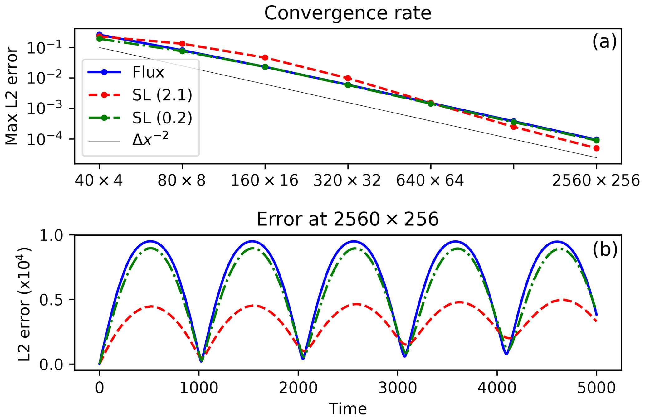
Figure 3 (a) Maximum L2 error, i.e. $(\int (\mathit{\sigma }-{\mathit{\sigma }}_{\mathrm{ex}}{)}^{\mathrm{2}}\mathrm{d}A/\left(L_x{L}_z\right){)}^{\mathrm{1}/\mathrm{2}}$, over the integration period for the test case of Sect. 3.3 vs. resolution for flux-form Eulerian advection with a Courant number of 0.2 (solid blue), semi-Lagrangian advection with a Courant number of 2.1 (dashed red), and semi-Lagrangian advection with a Courant number of 0.2 (dash-dotted green), showing second-order convergence (line). (b) L2 error over time for these algorithms, on the 2560×256 grid.

3.3.3 Results

The error over time of this test case is shown in Fig. 3. As expected, each method achieves second-order convergence. For the Eulerian advection control case, this is governed by its two-point central difference scheme. For the semi-Lagrangian cases, the dominant contribution to the error field comes from the lower-order vertical interpolation. While the semi-Lagrangian method has a higher order of accuracy for horizontal motion, here the problem is constructed such that horizontal and vertical motions are of equal importance.

As is often observed with semi-Lagrangian methods, the overall error of the scheme is somewhat lower for the high-CFL case than for the low-CFL case. The interpolation used to evaluate σ off the grid introduces error with each interpolation, and the overall contribution of this error necessarily scales in proportion to the number of interpolations and inversely with the time step size.

Overall, this simplified test case supports the conclusion that the semi-Lagrangian treatment of advection is a viable replacement for flux-form advection. The semi-Lagrangian method achieves similar (for low-CFL flows) or better (for high-CFL flows) error, and it remains stable for CFL values substantially larger than unity.

4 Trajectory calculation

With the mechanism for evaluating the f^B(x^D) term in Eq. (7) established in Sect. 3, the remaining half of the semi-Lagrangian advection algorithm is the estimation of the x^D departure points. This corresponds to the positions at the before time level (t₀−Δt) of those fluid parcels that will arrive on the reference grid x_ref the after time level (t₀+Δt). One such upstream location exists for each valid grid location, so in general x_d needs to be estimated for each t, u, and v point on the NEMO-OPA grid to provide for (respectively) the tracer and velocity advective forcings.

In general, calculation of the departure points is an implicit and nonlinear problem, requiring knowledge of the flow velocity at every subgrid place and time between the before and after time levels, before the flow at the latter has been computed. To make this problem tractable, we make a series of simplifying assumptions.

The first such assumption is to freeze the flow, such that trajectories are computed based on strictly the now velocities (that is, u, v, and w at the intermediate time level). This is consistent with the underlying leapfrog time-stepping algorithm and the other advection schemes in NEMO-OPA, where most fluxes are computed instantaneously with respect to the same now velocities. In physical terms, this constrains fluid parcels to follow paths based on estimated, instantaneous streamlines. In exchange, this decouples the trajectory computation from the after velocities and makes the process time explicit, which eliminates what would otherwise be a need to iterate the entire time-stepping process.

4.1 Exponential integration

Ordinarily, the next assumption in the trajectory calculation is to approximate the particle paths, either by a straight line or by a low-degree polynomial. In this case, the Lagrangian equation

$$\begin{array}{}\text{(28)}& {\displaystyle \frac{\mathrm{d}\mathit{x}}{\mathrm{d}t}}=\mathit{v}\left(\mathit{x}\right)\end{array}$$

is integrated with an approximate quadrature. Using the trapezoidal rule gives the approximation

$$\begin{array}{}\text{(29)}& {\mathit{x}}_{\mathrm{a}}-{\mathit{x}}_{\mathrm{d}}=\mathrm{\Delta }t\left(\mathit{v}\right({\mathit{x}}_{\mathrm{d}})+\mathit{v}({\mathit{x}}_{\mathrm{a}}\left)\right),\end{array}$$

where ${\mathit{x}}_{\mathrm{a}}=\mathit{x}(t_{\mathrm{0}}+\mathrm{\Delta }t)$ is the on-grid “arrival” point of the fluid parcel. This approximation is second-order in time, and it results in an iterative method where v(x_d) is interpolated, leading to a revised estimate of x_d.

Unfortunately, this approximation is not suitable for trajectory calculations in the general ocean because it does not appropriately handle flow near a solid boundary. Consider the case of two-dimensional flow in the positive half-plane, where fluid velocities are prescribed as $(u,v)=(x,-y)$. This forms an analytic continuation of flow near a boundary along the line x=0.

Now, apply equation Eq. (29) to the fluid parcel that arrives at ${\mathit{x}}_{\mathrm{a}}=(\mathrm{1},\mathrm{0})$. Along this streamline, v=0 by inspection so this equation reduces to one dimension and has the solution

$$\begin{array}{}\text{(30)}& x_{\mathrm{d}}={\displaystyle \frac{\mathrm{1}-\mathrm{\Delta }t}{\mathrm{1}+\mathrm{\Delta }t}}.\end{array}$$

For small values of Δt, this solution is reasonable. For Δt>1, however, this solution leads an unphysical trajectory, where the departure point is found to lie in the left half-plane (and thus lies inside the boundary).

The failure here is a specific example of Eq. (29) failing the Lipschitz trajectory-crossing criterion (Smolarkiewicz and Pudykiewicz, 1992), which requires $u_x\mathrm{\Delta }t<C\approx \mathrm{1}$. The trajectory implied by Eq. (30) crosses the trajectories of fluid parcels that arrive at ${\mathit{x}}_{\mathrm{a}}=(\mathrm{1}\pm \mathit{ϵ},\mathrm{0})$, and the resulting advection loses its physical meaning.

This trajectory-crossing criterion is a physical limit for solutions which develop discontinuous shocks, such as those that can arise in simulations of the nondispersive, nonlinear shallow water equations. However, these shocks are not typical of three-dimensional hydrostatic flows in the ocean, and they are certainly not universally seen at solid boundaries. The true trajectories of fluid parcels, if evaluated exactly, do not cross (and do not have origins inside the land domain), so a better approach is to directly integrate Eq. (28) without approximating the time derivative. Here, this one-dimensional system reduces to the ordinary differential equation

$$\begin{array}{}\text{(31)}& x_t=x,\end{array}$$

with the boundary condition $x(t_{\mathrm{0}}+\mathrm{\Delta }t)=x_a=\mathrm{1}$. The solution to this equation is obviously of the form x(t)=Cexp (t) for some constant C, and applying the boundary condition gives $x\left(t\right)=\exp (t-(t_{\mathrm{0}}+\mathrm{\Delta }t\left)\right)$ and a departure point of $x_{\mathrm{d}}=\exp (-\mathrm{2}\mathrm{\Delta }t)$.

This solution is very well behaved, lying exclusively in the right half-plane and asymptotically approaching the wall at x=0 as Δt→∞. This approach works when that of Eq. (29) fails because the direct integration properly captures the exponential-in-time path of the fluid parcel.

A generalization of this approach forms the basis for trajectory calculation in this work. Since the solution of Eq. (28) is not analytically possible with an arbitrary velocity field, we exactly solve Eq. (28) based on an approximate, linearly varying velocity field. This is similar to an approach discussed by Walters et al. (2007), where within a single, two-dimensional finite-element cell the linear velocity form is exactly given by the underlying discretization rather than an approximation.

Assume that an arbitrary fluid parcel arrives at x_a and that we know the velocity there (v_a) and at another point v(x_c)=v_c. We know that the fluid parcel must arrive at x_a travelling in the direction of ${\widehat{v}}_a={\mathit{v}}_a/{\mathit{\alpha }}_a$, with ${\mathit{\alpha }}_a=\Vert {\mathit{v}}_a\Vert$. Then v_c can be written in terms of this direction as ${\mathit{v}}_c={\mathit{\alpha }}_c{\widehat{v}}_a+{\mathit{\beta }}_c{\widehat{n}}_a$, for scalar α_c and β_c and some ${\widehat{n}}_a$ normal to ${\widehat{v}}_a$.

This forms a two-dimensional system spanned by vectors ${\widehat{v}}_a$ and ${\widehat{n}}_a$. If we additionally make the assumption that v(x) varies linearly in this plane, we can construct a simplified, two-dimensional coordinate system to solve Eq. (28). Here, the origin of the coordinate system corresponds to x_a, and the rotated coordinates $\widehat{x}$ and $\widehat{y}$ align with ${\widehat{v}}_a$ and ${\widehat{n}}_a$ respectively. This implies that x_c projects onto the point $({\mathit{x}}_c\cdot {\widehat{v}}_a,{\mathit{x}}_c\cdot {\widehat{n}}_a)=(x_c,y_c)$. The linearly interpolated velocities lie strictly in this plane, so the equations of motion for a fluid parcel are

$$\begin{array}{}\text{(32a)}& {\displaystyle }{x}_t& {\displaystyle }={\mathit{\alpha }}_a+({\mathit{\alpha }}_c-{\mathit{\alpha }}_a){\displaystyle \frac{x}{x_c}}\text{, and}\text{(32b)}& {\displaystyle }{y}_t& {\displaystyle }={\mathit{\beta }}_c{\displaystyle \frac{x}{x_c}},\end{array}$$

subject to the boundary condition that $x(t_{\mathrm{0}}+\mathrm{\Delta }t)=y(t_{\mathrm{0}}+\mathrm{\Delta }t)=\mathrm{0}$. Equation (32a) can be solved first, and applying the boundary condition $x(t_{\mathrm{0}}+\mathrm{\Delta }t)=\mathrm{0}$ gives

$$\begin{array}{}\text{(33a)}& x\left(t\right)={\displaystyle \frac{{\mathit{\alpha }}_a{x}_c}{{\mathit{\alpha }}_c-{\mathit{\alpha }}_a}}\left(\exp \right({\displaystyle \frac{{\mathit{\alpha }}_c-{\mathit{\alpha }}_a}{x_c}}(t-(t_{\mathrm{0}}+\mathrm{\Delta }t\left)\right))-\mathrm{1}).\end{array}$$

Applying this to Eq. (32b) along with its boundary condition $y(t_{\mathrm{0}}+\mathrm{\Delta }t)=\mathrm{0}$ gives

$$\begin{array}{ll}{\displaystyle }y\left(t\right)=& {\displaystyle \frac{{\mathit{\beta }}_c{\mathit{\alpha }}_a}{{\mathit{\alpha }}_c-{\mathit{\alpha }}_a}}\left({\displaystyle \frac{x_c}{{\mathit{\alpha }}_c-{\mathit{\alpha }}_a}}\right(\exp \left({\displaystyle \frac{{\mathit{\alpha }}_c-{\mathit{\alpha }}_a}{x_c}}\right(t-(t_{\mathrm{0}}+\mathrm{\Delta }t)\left)\right)-\mathrm{1})\\ \text{(33b)}& {\displaystyle }& {\displaystyle }-(t-(t_{\mathrm{0}}+\mathrm{\Delta }t\left)\right)).\end{array}$$

When the along-trajectory acceleration is small ($\left|\right({\mathit{\alpha }}_c-{\mathit{\alpha }}_a)\mathrm{\Delta }t/x_c|\ll \mathrm{1}$), Eq. (33) reduces to a trapezoidal rule with second-order accuracy in time.

4.1.1 Trajectory iteration

Evaluating Eq. (33) at $t=t_{\mathrm{0}}-\mathrm{\Delta }t$ and re-projecting the coordinates to the grid forms the basis of an iterative algorithm for trajectories.

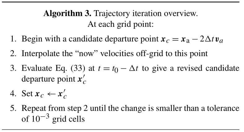
This algorithm is ideally suited to cases that look like flow away from a stagnation point, where a fluid parcel is accelerating as it reaches the grid point at t₀+Δt. In those cases, the $({\mathit{\alpha }}_c-{\mathit{\alpha }}_a)/x_c$ terms will be positive, and the exponential terms will limit the size of the trajectory for finite Δt. In the opposite case, however, the exponential terms will tend to lengthen the trajectory. For large Δt or large deceleration, this effectively demands that Eqs. (32)–(33) extrapolate beyond the velocity sample at x_c, a potential source of instability.

To remedy this, a limiter is added to step 3 of Algorithm 3, whereby x(t₀−2Δt) is constrained to the greater⁶ of that from Eq. (33a) and $-\mathrm{2}\mathrm{\Delta }tmax({\mathit{\alpha }}_a,{\mathit{\alpha }}_c)$. When limiting is necessary, it effectively reduces the time step used for the trajectory iteration, so for consistency a revised Δt^′ is computed by inverting Eq. (33a) with the limited $x_c^{\prime }$, which is then used to evaluate Eq. (33b).

4.2 Underrelaxation and land boundaries

While the construction of Algorithm 3 guarantees that trajectories cannot converge to an out-of-boundary point, there are no guarantees that the algorithm remains in boundary during the iteration process or that the iteration converges. The problem of a divergent or oscillatory iteration is more likely when the underlying velocity field does not resemble the linearly approximated velocity field integrated by Eq. (32), as then each iteration might result in very different approximations.

Addressing the latter point first, this work heuristically applies underrelaxation when Algorithm 3 is slow to converge. After 10 local iterations, step 3 is replaced by ${\mathit{x}}_c\leftarrow \frac{\mathrm{1}}{\mathrm{2}}({\mathit{x}}_c+{\mathit{x}}_c^{\prime })$; after 20 iterations the right-hand side becomes $\frac{\mathrm{1}}{\mathrm{4}}(\mathrm{3}{\mathit{x}}_c+{\mathit{x}}_c^{\prime })$, and after 30 iterations the right-hand side becomes $\frac{\mathrm{1}}{\mathrm{8}}(\mathrm{7}{\mathit{x}}_c+{\mathit{x}}_c^{\prime })$. At 40 iterations, the trajectory is truncated by ending the iteration with the first in-domain point returned from the process; this ensures some sort of advection even if the iterative process enters a limit cycle.

This underrelaxation also addresses the possibility that x_c might lie outside of the ocean domain. If x_c is masked, then there is no valid velocity to provide via off-grid interpolation, so instead of evaluating Eq. (33), ${\mathit{x}}_c^{\prime }$ is set to x_a in step 3 of Algorithm 3. This combines with the underrelaxation after 10 iterations to reduce the trajectory length until an in-boundary point is found, whereupon iteration resumes normally.

These values for iteration counts and underrelaxation parameters are conservatively specified. In the numerical tests discussed in this work, the vast majority of trajectories converge after one or two iterations, without needing to resort to underrelaxation or trajectory truncation.

4.3 Velocity interpolation

The trajectory algorithm requires the off-grid interpolation of velocities at each iteration. In principle, these velocities can be interpolated using the interpolation process of Sect. 3. Doing so would be ideal for ultimate consistency with the final off-grid interpolation, but this process is also computationally expensive. In practice, it is more efficient to evaluate the off-grid velocity field in step 2 of Algorithm 3 using trilinear interpolation; doing so causes little change in the numerical test cases in this work.

Trilinear interpolation proceeds with the same order of operations as Algorithm 1: velocities are first interpolated in depth to the (x,y) corners of the grid box at the off-grid level, then along the x direction, and finally along the y direction. Each individual interpolation respects the relevant boundary condition, so for example the u velocity is considered to reflect symmetrically around a boundary in y and z but is constrained to zero at a boundary in x.

One complication of linear interpolation, however, is that the velocity points are staggered by half a cell with respect to the physical boundary. In two dimensions, if the tracer point T(0,0) (to use grid-cell coordinates for the tracer grid denoted T) is a land point but T(0,1), T(1,0), and T(1,1) are all ocean points, then u-velocity point U(0,0) (denoting the u-velocity grid as U), halfway between T(0,0) and T(1,0), lies along the boundary. The boundary continues to U(0,0.5), whereupon U(0,0.5)–U(0,1) lies inside the ocean. This violates a basic assumption of linear interpolation, that the velocity should vary smoothly (and approximately linearly) within the u cell.

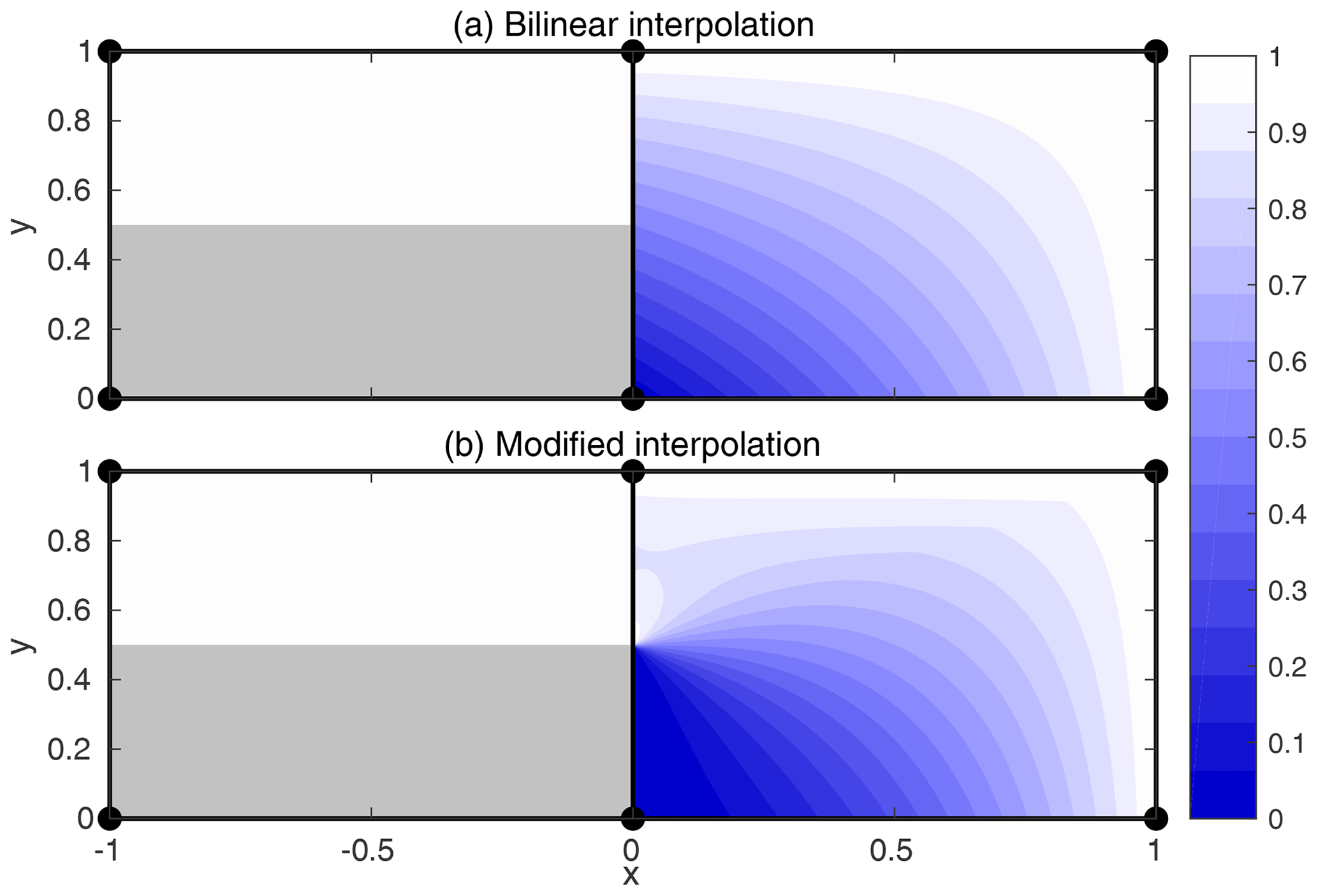
Figure 4 Illustration of modified linear interpolation near corners. In (a), linear interpolation results in an interpolated velocity field that does not respect the boundary conditions along $\mathrm{0}<y<\mathrm{0.5}$ and a discontinuous interpolated field at $\mathrm{0.5}<y<\mathrm{1}$. In (b), modifying the linear interpolation with a corner solution results in a field that respects the boundary condition.

This causes two problems for trajectory computation. The first problem is that after repeated one-dimensional interpolation, the boundary condition is no longer necessarily respected by the interpolated velocity, which can result in a trajectory iteration that “pushes” the departure point into the wall, causing non-convergence. The second problem is that while the interpolation process guarantees continuity of the interpolated field at the cell corners, the boundary conditions can cause large discontinuities along the cell edges, again resulting in a convergence failure. In the above example, the interpolated velocity at $U(+\mathit{ϵ},\mathrm{0.6})$ would be influenced by both U(0,1) and the zero velocity at the physical boundary of U(0,0), but the interpolated velocity at $U(-\mathit{ϵ},\mathrm{0.6})$ would be influenced by U(0,1) and its reflection at a ghost point. These problems are illustrated in Fig. 4a.

The solution to both of these problems is to blend the linearly interpolated function with a corner singularity solution. A bilinear function is a solution to Laplace's equation (∇²f=0), so it is reasonable to consider corner solutions that are also solutions to Laplace's equation.

Without loss of generality, consider a grid cell defined by $(x,y)\in [\mathrm{0},\mathrm{1}{]}^{\mathrm{2}}$, such that there is a solid boundary along $(x=\mathrm{0},y<\mathrm{0.5})$ as depicted in Fig. 4. Treating the boundary as an infinite half-plane, with $f(\mathrm{0},y)=\mathrm{0}$ for y<0.5 and $f(\mathrm{0},y)=f(\mathrm{0},\mathrm{1})$ for y>0.5, the “corner” solution to Laplace's equation is

$$\begin{array}{}\text{(34)}& f_{\text{corner}}(x,y)={\displaystyle \frac{f(\mathrm{0},\mathrm{1})}{\mathrm{2}}}(\mathrm{1}+\cos ({\tan }^{-\mathrm{1}}\left({\displaystyle \frac{y-\mathrm{0.5}}{x}}\right)\left)\right),\end{array}$$

while bilinear interpolation would give

$$\begin{array}{}\text{(35)}& \begin{array}{rl}{f}_{\text{bilinear}}(x,y)=& (\mathrm{1}-x)yf(\mathrm{1},\mathrm{0})+x(\mathrm{1}-y)f(\mathrm{0},\mathrm{1})\\ & +xyf(\mathrm{1},\mathrm{1}).\end{array}\end{array}$$

These two solutions are blended together, with Eq. (34) taking precedence along the solid boundary (x=0 and $\mathrm{0}\le y\le \mathrm{0.5}$) and Eq. (35) taking precedence along the x=1 and y=1 boundaries of the cell. This gives

$$\begin{array}{ll}{\displaystyle }{f}_{\text{blend}}(x,y)=& {\displaystyle }\mathit{\sigma }(x,y)f_{\text{bilinear}}(x,y)\\ \text{(36)}& {\displaystyle }& {\displaystyle }+(\mathrm{1}-\mathit{\sigma }(x,y\left)\right)f_{\text{corner}}(x,y),\end{array}$$

where $\mathit{\sigma }=max(\mathrm{1}-x,\mathrm{2}(y-\mathrm{0.5}\left)\right)$.

The blended function exactly respects the solid boundary condition, and the discontinuity at the cell edges is significantly reduced. Blended functions for other configurations of the solid wall are given by applying the appropriate reflections and rotations to Eq. (36).

5 Results

5.1 Flow past an island

To demonstrate the impacts of semi-Lagrangian advection on a simple test case with a lengthened time step, we first present the quasi-two-dimensional test case of isothermal flow past an interposed island.

This test case consists of a $\mathrm{280}\times \mathrm{70}\times \mathrm{3}$ point grid, with grid resolution $\mathrm{\Delta }x=\mathrm{\Delta }y=\mathrm{5}\mathrm{m}$ and Δz=10 m. A 50 m×50 m region (10 points ×10 points) is masked as land in the middle of the domain. The inflow boundary condition is set to $u=\mathrm{0.03}\mathrm{m}{\mathrm{s}}^{-\mathrm{1}}$, v=0; this was also imposed throughout the domain as an initial condition. The reference frame was also irrotational, with a Coriolis parameter of 0.

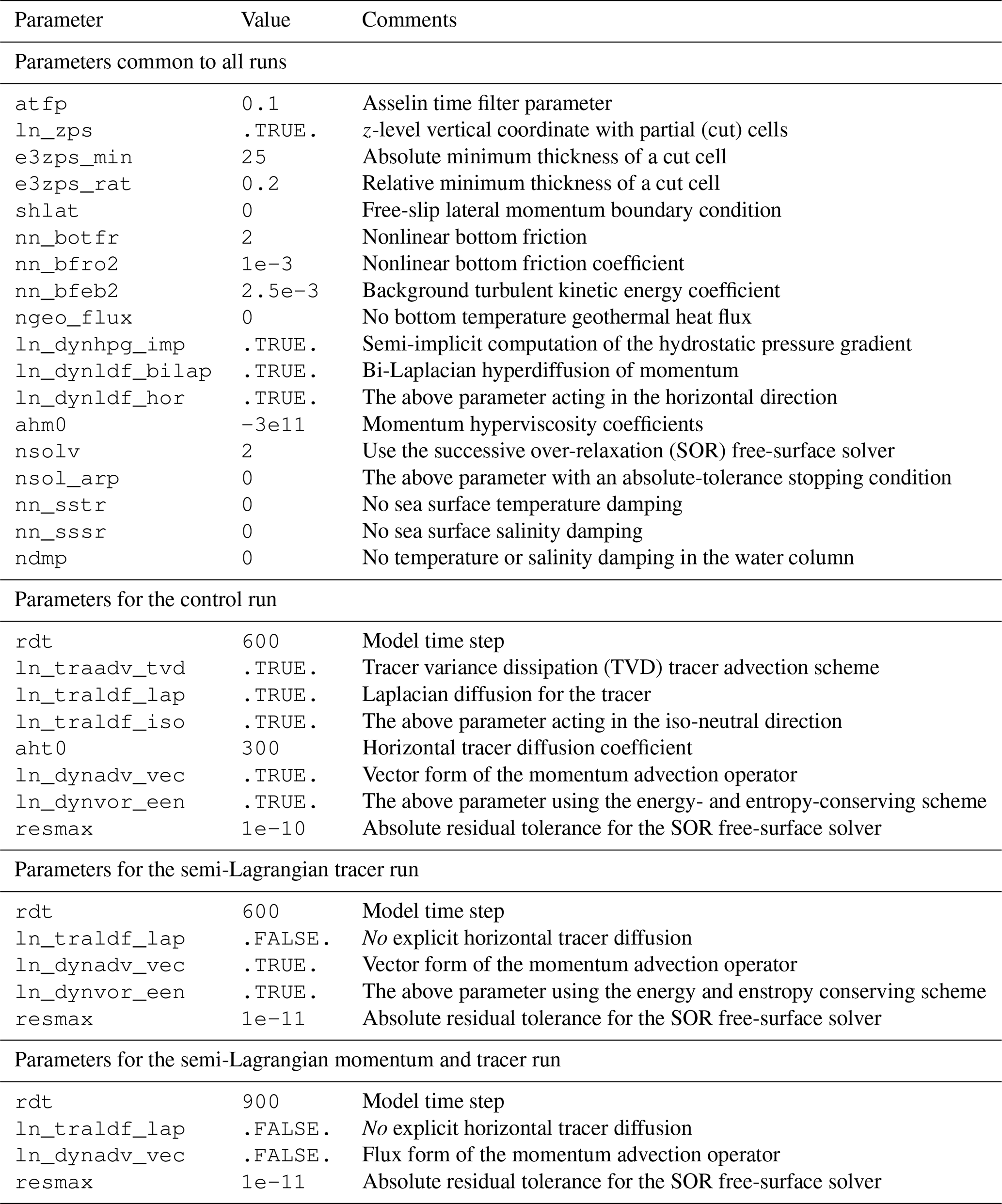
Relevant namelist parameters are given in Table 1, with parameters that differ between the control and semi-Lagrangian runs highlighted. The control run used flux-form velocity advection⁷ via the QUICKEST scheme (Leonard, 1979, 1991), whereas the semi-Lagrangian run used semi-Lagrangian advection of momentum in flux form as described in Sects. 3 and 4. To emphasize the dynamical differences between the advection schemes, both test cases were run with no explicit horizontal diffusion of momentum. Vertical mixing terms, largely irrelevant for this quasi-two-dimensional case, were set consistently with the ORCA025 simulations in Sect. 5.2.

Both series of runs used the implicit free-surface formulation (enabled with the compile-time key key_dynspg_flt), which damped the large initial surface gravity waves caused by the imposition of the blocking island on the steady-state flow.

Table 1 Selected namelist parameters for the test case of Sect. 5.1.

After the initial gravity-wave adjustment, this test case quickly develops a set of recirculating vortices in the lee of the island. Over time these vortices grow in extent and would begin detaching to form a vortex street, but this does not happen before the 8000 s end of the simulation. Although there is no explicit horizontal diffusion of momentum in these runs, the flow regime is much more laminar than would be implied by the physical Reynolds number of 1.5×10⁶, based on the free-stream velocity, edge-length of the island, and molecular viscosity of water.

In moving around the box, the flow locally accelerates to a maximum steady velocity of about 0.05 m s⁻¹, and this maximum velocity is reached in the vicinity of the leading-edge corners of the box. The exact value of this maximum depends on both the simulation time and the time step, but our expected pattern holds: the control simulation is stable with a time step of 64 s, which corresponded to a maximum steady Courant number, i.e. $max\left(u_{\text{steady}}\right)/\mathrm{\Delta }x$, above 0.6 (and a maximum transient CFL of 0.95), but it is unstable with a time step of 80 s.

Semi-Lagrangian advection maintains stability for much longer time steps. Figure 5 shows the free-surface height and flow streamlines for Δt between 5 and 160 s, and only the semi-Lagrangian method remains stable for 80 and 160 s time steps. For both advection schemes, the longer time step is associated with a more diffuse flow pattern, with lengthening (and less intense) recirculating vortices in the lee of the island.

This effect is stronger with semi-Lagrangian advection than with Eulerian advection. We attribute this to the nature of the flow at the leading edge of the island. Here, the dominant flow balance is cyclostrophic, where the pressure gradient at these corners balances the local vorticity. The operator splitting method used here treats the advective terms in a frame following the flow, but it can only apply the pressure force at the destination cell. This results in an inconsistency that grows with Δt, related to the forces in equation Eq. (2) being available only at the endpoint of the Lagrangian trajectory – an O(Δt) approximation to the integral.

This inconsistency is most evident in the 160 s time step case (bottom panel in Fig. 5b), where the maximum steady Courant number of 1.6 implies that fluid parcels are advected by about three grid cells over the 2Δt leapfrog step. There, the lowest pressure region at the leading edge of the flow has moved slightly further downstream.

In the full ocean, the geostrophic effect predominates, with a leading-order balance between the pressure gradient and the Coriolis force (planetary vorticity), so we expect this issue to be less pronounced.

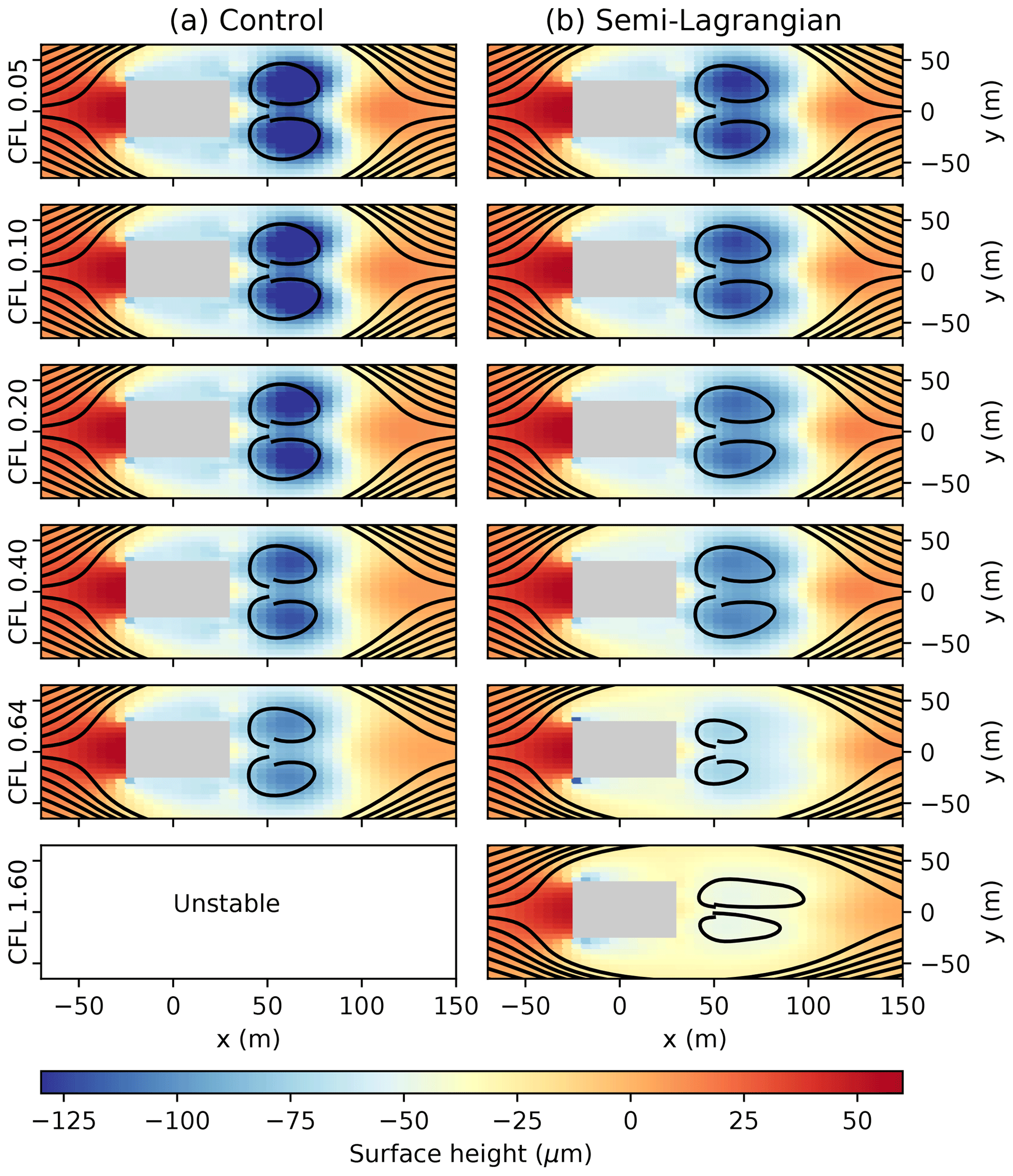
Figure 5 Free-surface height and streamlines for the test case of Sect. 5.1, after 8000 s for Δt=5, 10, 20, 40, 64, and 160 s (top to bottom, with the approximate Courant number listed). Results for the Eulerian advection scheme are shown in (a), and results for the semi-Lagrangian advection of momentum are shown in (b). As the time step increases both advection schemes show more diffuse behaviour; however the semi-Lagrangian advection scheme remains stable to Δt=160 s, whereas the Eulerian scheme becomes unstable after Δt=64 s.

5.2 Global forced runs

To evaluate semi-Lagrangian advection in a more realistic forecasting setting, we conducted a preliminary series of free runs of the NEMO-OPA model. The runs consisted of the following:

• a control run, based on the configuration of Environment and Climate Change Canada's $\mathrm{1}/\mathrm{4}{}^{\circ }$ nominal-resolution Global Ice/Ocean Prediction System (GIOPS) (Smith et al., 2016) with a 10 min model time step;⁸ tracers were advected with the model's tracer variance dissipation scheme (Lévy et al., 2001), and momentums were advected in vector form with the model's energy and enstrophy conserving scheme⁹ (Arakawa and Lamb, 1981);

• a “semi-Lagrangian tracer” run, where momentum was advected as in the control scheme and the semi-Lagrangian advection described in this work was used for advection of salinity and temperature; additionally, this run disabled horizontal diffusion of salinity and temperature; and

• a “semi-Lagrangian momentum and tracer” run, where momentum as well is advected with the semi-Lagrangian scheme; the configuration was otherwise the same as the semi-Lagrangian tracer run, save for a 15 min model time step.

The runs were all initialized at 1 October 2001 on the ORCA025 grid. The ocean was at rest, and temperature and salinity were given by the 2011 World Ocean Atlas climatology (Locarnini et al., 2013; Zweng et al., 2013). Atmospheric forcing was provided at 1 h intervals from Environment and Climate Change Canada's $\mathrm{1}/\mathrm{4}{}^{\circ }$ global atmospheric reforecast, and sea ice was modeled via coupling with version 4.0 of the CICE model (Hunke and Dukowicz, 1997), with dynamically active (moving) ice. Selected namelist parameters are provided in Table 2.

As with Sect. 5.1, the test cases used NEMO-OPA's linear free-surface with a time-implicit solver, and tidal forcing was not present in these configurations. In a typical time step, the vast majority of semi-Lagrangian trajectories converged in one iteration (mean 1.004 over the semi-Lagrangian tracer run). A very small minority of cells required an extended number of iterations or underrelaxation as described in Sect. 4.2, but this did not affect the overall trajectory-calculation performance because convergence was measured (and iterations limited) on a per-cell basis.

Each run continued through late 2009. For reasons of space efficiency, we recorded the two-dimensional sea surface height, temperature, and salinity fields for each model day, and we preserved every fifth daily-mean, three-dimensional output of temperature, salinity, and horizontal ocean velocity.

Table 2 Selected dynamical and numerical namelist parameters for the test cases of Sect. 5.2.

For short- and medium-term forecasts, the operational coupled forecasting systems at CMC are constrained by observations and periodic re-initialization. With a focus on this forecasting horizon, the objectives of these long free-runs were as follows:

• to provide a test of model stability with semi-Lagrangian advection, in terms of both avoiding crashes and providing plausible ocean fields;

• to check for any large-scale conservation errors, which might be difficult to correct given the sparsity of observation data for the deep ocean; and

• to note any qualitative improvement or deterioration in the effective resolution of the model.

This first goal of model stability was met in part by the successful completion of these runs. Use of semi-Lagrangian advection for both tracers and momentum allowed us to increase the effective time step from 10 min (with typical maximum Courant number¹⁰ of 0.2, found in the vertical direction) to 15 min (Courant number 0.3). Further increases led to instability and model crashes not from the advection component, but from the ice model. In this version of the model, the ocean–ice stress is coupled in a time-explicit way between the water and ice components. Concurrent work towards a time-implicit coupling has given encouraging preliminary results on further time step increases.

The use of semi-Lagrangian advection also gives global flows qualitatively similar to the control run, and average transports in the Atlantic overturning circulation and Circumpolar current are comparable between the control and semi-Lagrangian runs (Fig. 6). The semi-Lagrangian runs appear to result in a slightly weaker overturning circulation and a slightly stronger circumpolar current than the control run, but these results may not be robust to retuned physical parameterizations. Using semi-Lagrangian advection for the velocity components results in a significant decrease to overall ocean kinetic energy (Fig. 7), both during and after the spin-up period.

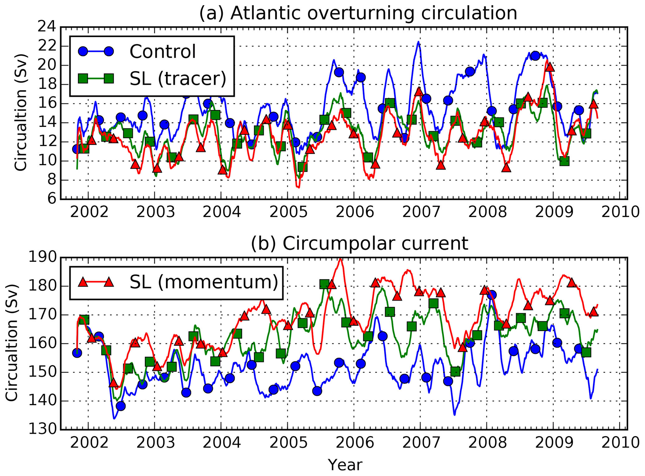
Figure 6 (a) The 61 d mean transports for the Atlantic overturning circulation (net northward flux above 1000 m depth at 27.25^∘ N latitude in the Atlantic Ocean) and (b) Antarctic circumpolar current (net eastward flux at 67.75^∘ W longitude in the Drake Passage) over time for the test cases of Sect. 5.2

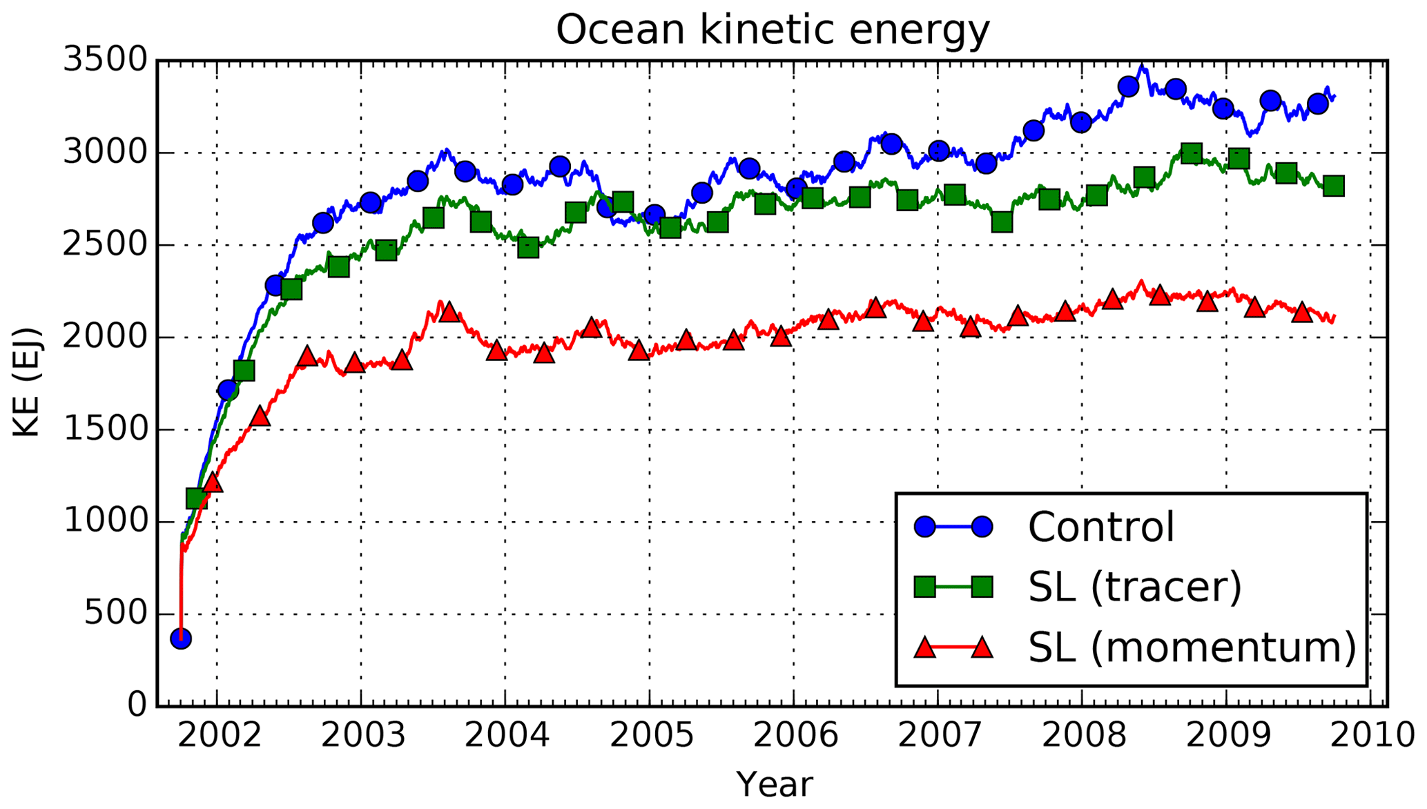
Figure 7 Total ocean horizontal kinetic energy (EJ) over time for the test cases of Sect. 5.2. All of the test cases generally reproduce the monthly to yearly variability in kinetic energy, but the use of semi-Lagrangian momentum advection results in significantly lower total kinetic energy.

The cause of this energy disparity is under investigation, but we believe the most likely cause is the application of slope limiting to the u and v fields independently. Future work will focus on taking a more nuanced approach to filtering, but this effect may not be very significant in a shorter-term forecast setting with frequent re-initializations from an analysis.

The second goal of global conservation was met. Although semi-Lagrangian advection does not guarantee conservation of tracers, the impact on the global balance of temperature and salinity was small. Figure 8 shows the evolution of ocean-average temperature and salinity over time in these runs, and the effect of non-conservation attributable to the semi-Lagrangian advection of tracers is comparable to the magnitude of uncertainty in the global balance of atmospheric forcing – the imbalance seen in the control run. Each case saw an overall temperature drift of about 0.04 K over the simulated period, with the semi-Lagrangian cases having a slight warming trend against the control run's slight cooling trend, and all three runs showed a very small increase in ocean-average salinity, by about 0.01 PSU.

The temperature change vs. depth over the simulated period is shown in Fig. 9. Both the control and semi-Lagrangian runs showed a warming trend in the surface layers, but the semi-Lagrangian runs showed temperature stability in fluid layers below 1000 m depth, whereas the control run showed a cooling trend in these waters.

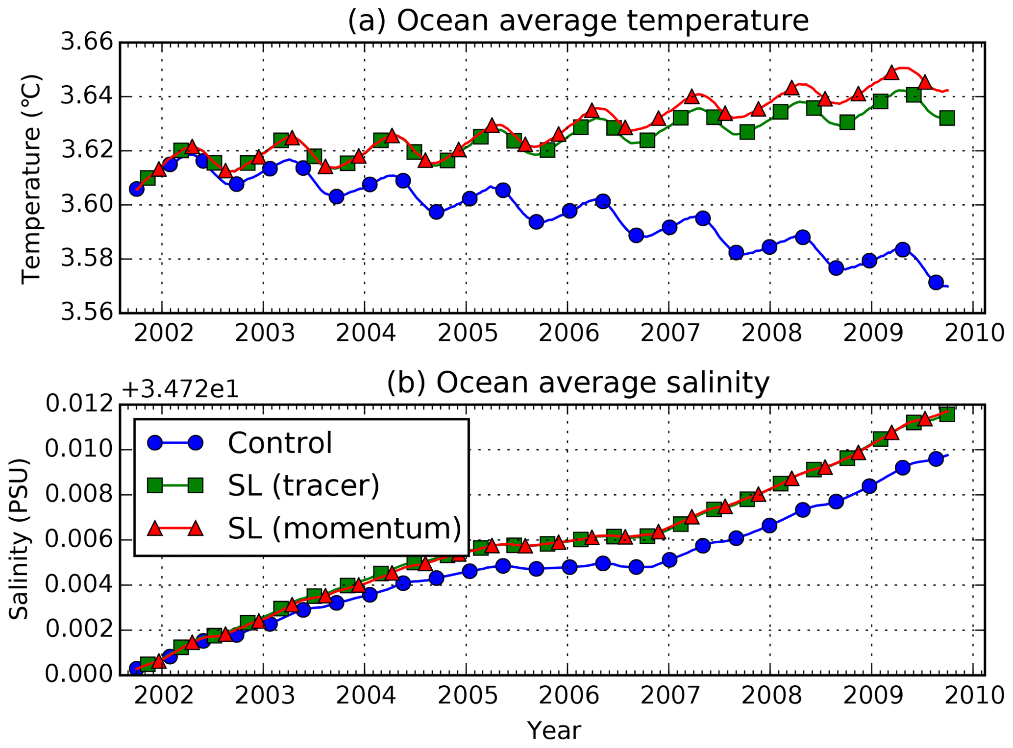
Figure 8 (a) Ocean-average temperature (^∘C) and (b) salinity (PSU) over time for the test cases of Sect. 5.2. Although conservation is not guaranteed by semi-Lagrangian advection, long-term trends are similar between the semi-Lagrangian runs and the control run.

Figure 9 (a) Initial ocean-average temperature profile (^∘C) vs. depth and (b) change at the end of the simulated period (4 October 2009) for the test cases of Sect. 5.2. Both semi-Lagrangian runs show temperature stability in deeper waters, whereas the control run shows a small cooling.

Despite the energy shortfall with semi-Lagrangian advection of momentum, we see tentative signs that the method increases the model's effective resolution. Figure 10 shows one particular sea surface temperature realization, from the 31 December 2005 of each test case, along with the magnitude of the temperature gradient. The large-scale flows are similar between the control and semi-Lagrangian runs (and most similar between the control and semi-Lagrangian tracer run), but the semi-Lagrangian runs have noticeably stronger gradients in the sea surface temperature, in patterns that resemble smaller-scale eddies.

Figure 10 (a, c, e) Sea surface temperature and (b, d, f) the magnitude of its gradient for the (a, b) control, (c, d) semi-Lagrangian tracer, and (e, f) semi-Lagrangian momentum and tracer test cases of Sect. 5.2, for 31 December 2005 in the Labrador Sea. Although the large-scale flows are similar, the runs with semi-Lagrangian advection of tracers have noticeably more fine-scale variability.

6 Conclusions and further work

This work has derived a semi-Lagrangian advection scheme for the NEMO-OPA model. After advecting a tracer or momentum field along estimated fluid parcel trajectories, it calculates a time trend to provide to the remainder of the model; in this way the semi-Lagrangian scheme serves as a drop-in replacement for other tracer and (flux-form) momentum schemes.

The development of this advection module relied on several new or newly applied algorithms that might be relevant to other ocean models or other domains:

• The “semi-Lagrangian trend” form of equation Eq. (7) might be useful in other models when researchers wish to implement semi-Lagrangian advection after the fact, without disrupting the calculation of other forcing terms.

• The Hermite interpolation form in Sect. 3, especially combined with the C¹-continuous estimate of the vertical derivative in Sect. 3.2 might find application in other domains where, as in the ocean, one dimension (the vertical) is more oscillatory than others.

• The exponential integration of trajectories in Eq. (4) may be useful in other applications that feature strong accelerations over trajectories. In particular, it forbids trajectory-crossing in one-dimensional flows, and here that property ensures that trajectories remain inside the ocean domain.

• The “corner solution” treatment of velocity for trajectory calculations near corners might find use in other applications with staggered velocity components.

Overall, we find that the semi-Lagrangian method is effective at extending the realizable time step in the NEMO-OPA model. In the simple domain of Sect. 5.1, this method resulted in a stable simulation with advective Courant numbers in excess of 1. Although we only extended the time step from 10 to 15 min for the semi-Lagrangian momentum run in Sect. 5.2, this limitation was imposed by the ice model. Disabling ice dynamics allowed us to increase the time step to 30 min, but this would have made the results incomparable with those of the control and semi-Lagrangian tracer runs. Preliminary work with the CICE sea model and implicit coupling of the ice–ocean stress seems to allow us to relax the ice-related time step restriction.

6.1 Performance and implementation

In spite of this increased time step, the semi-Lagrangian method by itself does not yet improve overall computational performance. The semi-Lagrangian momentum and tracer run of Sect. 5.2 took approximately 1 h of computational time per 5 d of simulated time, using 128 Intel Xeon E5530 processors at 2.4 GHz. With a 10 min time step, the semi-Lagrangian tracer run took approximately 50 min for the same 5 d of simulated time, whereas the control run took just 30 min. We expect these results to improve with further numerical optimization work. In particular, we did not take great care to ensure that loops were vectorized where possible, and it is much more difficult for compilers to automatically vectorize the point-by-point semi-Lagrangian computations compared to volume flux calculations in the traditional advection schemes.

About one-third of the additional computational cost comes from trajectory iterations, and the remainder comes from the cubic interpolation. This suggests that the relative cost of semi-Lagrangian advection will be lower than presented here if trajectories can be reused for multiple tracer species (such as biogeochemical constituents). Additionally, it suggests that a further optimization may be to reuse tracer trajectories for momentum advection, at least away from the boundaries where interpolating (staggering) trajectories might be reasonable. It seems unlikely that optimization will reduce the per-time-step penalty to the 20 % value seen by Ritchie et al. (1995) for an atmospheric model – owing to the lack of three-dimensional implicit equations and expensive physical parameterizations elsewhere in NEMO-0PA – but we are hopeful that semi-Lagrangian advection will nonetheless improve overall system performance.

The parallel (MPI) implementation of this algorithm was straightforward. With the relatively modest increase in Courant number for the cases in this work, we simply needed to increase the interprocessor lateral halo (parameters jpreci and jprecj) to three points, which was sufficient to allow a fluid parcel arriving at a processor's edge to apply the full interpolating stencil for the Courant numbers reached in the presented simulations. This increase in halo size was small compared to the processor tile size of about 50×260 grid points for the runs in Sect. 5.2. Extending this to support very large horizontal Courant numbers, however (if another solution could be found to stabilize baroclinic waves), would require either prohibitively large halo sizes or additional interprocessor communication to track fluid parcels that cross MPI boundaries.

6.2 Qualitative comments on results

Although the semi-Lagrangian method does not guarantee tracer conservation, we see no evidence that its implementation here leads to a degradation relevant in a weekly to seasonal forecast setting. In particular, the deep-water temperature stability shown in Fig. 9 is an encouraging sign that semi-Lagrangian advection will preserve the deep-water structure that is weakly constrained by data. Even small imbalances, however, might become significant over the decade-to-century timescales of climate simulations. Further work will be necessary to characterize this method before we can safely recommend semi-Lagrangian advection in such settings.

For the test cases in Sect. 5.2, semi-Lagrangian advection of tracers appears to slightly increase the effective resolution of the model. However, this effect is much more mixed when momentum is also advected with the semi-Lagrangian method, in part because the underlying currents differ. Both of these differences will be the subject of future study, with the specific intention of assessing these effects in the setting of shorter-term forecasts. We speculate that the overall loss of kinetic energy with semi-Lagrangian advection of momentum is attributable to the use of the slope limiter: limiting each component of velocity separately may be causing unrealistic diffusion of smaller-scale structures in the presence of background vorticity. We hope to address this issue with more selective limiting.

6.3 Future development

Finally, the development in this paper implicitly assumes that the coordinate system is static with time. This is not the case in NEMO-OPA when using its nonlinear free-surface option, which necessarily implies time-varying vertical levels. Adapting the semi-Lagrangian method to this more general coordinate system will be a focus of future work, which will be required to apply this advection scheme to higher-resolution domains that require tide-permitting simulations.

Additionally, future versions of NEMO intend to move to a third-order Runge–Kutta time-stepping algorithm (Shu and Osher, 1997), which constructs a full time step as a linear combination of forward Euler steps. We expect that the semi-Lagrangian “advective trend” of Eq. (7) can be adapted to this framework in a straightforward manner by basing the calculated trend on the current-step values of tracers and velocities, but the adaptation may require care to preserve the higher-order temporal accuracy of the overall scheme.