the Creative Commons Attribution 4.0 License.
the Creative Commons Attribution 4.0 License.
 | 05 Aug 2020
Numerical study of the seasonal thermal and gas regimes of the largest artificial reservoir in western Europe using the LAKE 2.0 model
Victor Stepanenko
Rui Salgado
Miguel Potes
Alexandra Penha
Maria Helena Novais
Gonçalo Rodrigues
The Alqueva reservoir (southeast of Portugal) is the largest artificial lake in western Europe and a strategic freshwater supply in the region. The reservoir is of scientific interest in terms of monitoring and maintaining the quality and quantity of water and its impact on the regional climate. To support these tasks, we conducted numerical studies of the thermal and gas regimes in the lake over the period from May 2017 to March 2019, supplemented by the data observed at the weather stations and floating platforms during the field campaign of the ALentejo Observation and Prediction (ALOP) system project. The 1D model, LAKE 2.0, was used for the numerical studies. Since it is highly versatile and can be adjusted to the specific features of the reservoir, this model is capable of simulating its thermodynamic and biogeochemical characteristics. Profiles and time series of water temperature, sensible and latent heat fluxes, and concentrations of CO2 and O2 reproduced by the LAKE 2.0 model were validated against the observed data and were compared to the thermodynamic simulation results obtained with the freshwater lake (FLake) model. The results demonstrated that both models captured the seasonal variations in water surface temperature and the internal thermal structure of the Alqueva reservoir well. The LAKE 2.0 model showed slightly better results and satisfactorily captured the seasonal gas regime.
- Article
(6868 KB) - Full-text XML
-
Supplement
(621 KB) - BibTeX
- EndNote


Inland water bodies are active and simultaneously sensitive regulators of the weather and climate processes of the Earth, and changing the temperature, wind, precipitation in the surrounding areas; their thermal and gas regimes, in turn, can serve as a response to the ecosystem status or climate change (Bonan, 1995; Adrian et al., 2009; Samuelsson et al., 2010). In modern climate and/or weather models, lakes and reservoirs are large-scale structures and are taken into account explicitly (Bonan, 1995); their parameterizations are intensively embedded in these models (Salgado and Le Moigne, 2010; Dutra et al., 2010; Subin et al., 2012). The 1D lake models, e.g. the freshwater lake (FLake) model (Mironov et al., 2010), the Dynamics Reservoir Simulation Model (DYRESM; Imberger and Patterson, 1981), and the generalized linear model (GLM; Hipsey et al., 2019), play a major role in this process. Their simplicity, computational efficiency, and reliability of the simulation results allow them to be used not only in studies of the dynamics of single lakes but also in the climate-related tasks of long-term numerical simulations, where vast territories with huge numbers of water bodies should be taken into account. As a result, the number of numerical studies connected with the vertical thermodynamics and biogeochemistry of lakes and their interaction with the atmosphere increases (Thiery et al., 2014; Heiskanen et al., 2015; Le Moigne et al., 2016; Ekhtiari et al., 2017; Su et al., 2019).
A realistic representation of the thermal and gas regimes of lake models is important for solving current and prognostic tasks. For example, a high accuracy of the calculations of sensible and latent heat fluxes, momentum, and water surface temperature is required for atmospheric models in which these parameters are the boundary conditions (Bonan, 1995; Mironov et al., 2010; Dutra et al., 2010; Salgado and Le Moigne, 2010; Balsamo, 2013). On the other hand, an adequate simulation of the water temperature profiles would be a very interesting new output of weather prediction and earth system models because temperature is a key factor for lake ecosystem processes. This information might be useful for water quality management and for better representation of the gas emissions (CO2, O2, and CH4) from lakes to the atmosphere, which are relevant to various atmospheric processes (Walter et al., 2007).
Fully filled only in 2004, the Alqueva reservoir is in the spotlight of many studies connected with its ecosystem services and ecology (Penha et al., 2016; Tomaz et al., 2017; Pereira et al., 2019), water quality (Potes et al., 2011, 2012, 2018; Novais et al., 2018), and lake–atmosphere interactions (Lopes et al., 2016; Policarpo et al., 2017; Potes et al., 2017; Iakunin et al., 2018). The aim of the present work is a numerical study of the seasonal variations in the thermal and gas regimes of the reservoir, which was held under the ALentejo Observation and Prediction (ALOP) system project in which an extensive field campaign and lake model simulations were combined. For the latter, we used the 1D model, LAKE 2.0 (Stepanenko et al., 2016), that features the biogeochemical block that simulates the concentrations of O2, CO2, and CH4 in water. In addition, the FLake model, which is well established in weather and climate studies, was used as a reference to compare the results of the thermodynamic characteristics of the reservoir. Before starting the numerical simulations, the LAKE 2.0 model was adapted to the features of the Alqueva reservoir, including the introduction of the realistic values of the water pH and light extinction coefficients and adequate value of the coefficient of the hypolimnion turbulent mixing rate. Both models were forced with the observed meteorological data at the reservoir, which contributed to increasing the reliability of the results. The simulation covered the period from May 2017 to April 2019, and its results and the possibility of applying the LAKE 2.0 model in the operational mode might be used in future studies of weather and climate and biochemical-related tasks.
2.1 Object of study
The Alqueva reservoir is located in the southeast of Portugal, spreading over 83 km in the former valley of the Guadiana River (Fig. 1).
Established in 2002 to meet the region's water and electricity needs, its surface covers an area of 250 km2, the maximum depth is 92 m, the average depth is 16.6 m, and the storage capacity of water is estimated at 4.15 km3, which makes it the largest reservoir in western Europe.
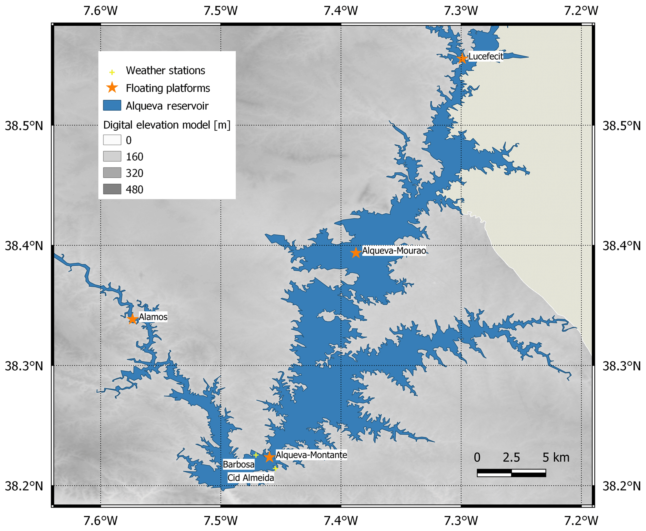
Figure 1Location of the Alqueva reservoir and ALentejo Observation and Prediction (ALOP) stations. The map was built using the digital elevation model of the ASTER Global Digital Elevation Model (GDEM) version 2 (https://asterweb.jpl.nasa.gov/gdem.asp, last access: 1 August 2020).
Long periods of drought that could last for more than 1 consecutive year (Silva et al., 2014) are typical in this part of the Iberian Peninsula. The Alqueva region is characterized by a hot Mediterranean summer climate (Csa type, according to the Köppen climate classification), with a small area that has a semi-arid climate (BSk type). In summer, the maximum daily air temperature ranges between 31 and 35 ∘C (July and August) while the record values may reach 44 ∘C. The winter period (December–February) in the region is relatively mild and wet, with an average air temperature of 10.3 ∘C. Nevertheless, even in January the air temperature can reach a maximum value of 24 ∘C during long periods of stable conditions when the Azores anticyclone settles into a favourable position. Seasonal rainfall normally occurs between October and May. The annual average values of the accumulated precipitation (1981–2010 normals from http://www.ipma.pt, last access: 1 August 2020) registered at the weather station in Beja, located 40 km away from the reservoir, is 558 mm. Mean daily values of the incident solar radiation at the surface are about 300 W m−2 (one of the highest in Europe) and the daily maximum in summer often may exceed 1000 W m−2 (Iakunin et al., 2018).
2.2 Observed data
Geographical and climatological factors make the Alqueva reservoir a vital source of fresh water that is needed to support the population and economy in the region, while on the other hand, increasing anthropogenic and heat stress negatively affects the lake's ecosystem (Penha et al., 2016). Monitoring the quantity and quality of water in the reservoir has become an essential scientific task. This task is addressed in the framework of the ALOP project that is related to the observations and numerical experiments on the study of the processes of the atmosphere called the Alqueva reservoir system. Models of different spatial and timescales were used in the ALOP numerical experiments.
The ALOP field campaign was focused on measurements of physical, chemical, and biological parameters in the water and air columns at the water–atmosphere interface and on the shores of the reservoir. In the present work, the following facilities were used and equipped to obtain the required data for the numerical simulations during the field campaign: four floating platforms (namely, Montante, Mourão, Alamos, and Lucefécit) and two dedicated weather stations in the margins (namely, Barbosa and Cid Almeida); their locations are marked with circles in Fig. 1. The principal scientific site on the lake is the Montante floating platform, which is located in the southern and deeper part (74 m) of the reservoir (38.2276∘ N, 7.4708∘ W). The following equipment was deployed on the platform and continuously provided measurements during the whole field campaign:
-
an eddy-covariance system (Campbell Scientific) provides data of atmospheric pressure, air temperature, water vapour and carbon dioxide concentrations, 3D wind components, linear momentum, sensible heat, latent heat, and carbon dioxide fluxes;
-
an albedometer (model CM7B; Kipp & Zonen) and a pyrradiometer (type 8111; Philipp Schenk GmbH) was used in order to measure upwelling and downwelling shortwave and total radiative fluxes;
-
a set of 14 probes (107 temperature probe; Campbell Scientific) measured the water temperature profile at the following depths, namely 5, 25, and 50 cm, and 1, 2, 4, 6, 8, 10, 12, 15, 20, 30, and 60 m.
Two probes were installed at the platform to assess water quality. A multiparametric probe (Aqua TROLL 600; In-Situ Inc.) that provided information about dissolved oxygen concentration and pH values, among other parameters, was mounted on the platform at a 25 cm depth on 3 July 2018 and worked until the end of the campaign. It was also used to make profiles during regular maintenance visits to the platform. A Pro-Oceanus Mini CO2 analogue output probe was also mounted on the platform at a 25 cm depth to measure the dissolved CO2 concentration continuously and was occasionally used to collect vertical profiles. Installed in the beginning of the campaign, the probe was working until the middle of June 2017 when it failed. It was repaired and reinstalled in October 2017, but another problem occurred in November and probe was removed for the remainder of the study.
Two land weather stations (namely, Barbosa and Cid Almeida) were installed on opposite shores with the floating platform in the middle, between them (38.2235∘ N, 7.4595∘ W and 38.2164∘ N, 7.4545∘ W, respectively; green circles in Fig. 1). The equipment of both weather stations is listed in Table 1. Data from the Montante floating platform, Barbosa, and Cid Almeida weather stations were automatically downloaded and transferred daily to the server in the Institute of Earth Sciences (ICT) at the University of Évora. An important part of the campaign were the regular field trips to the reservoir for the cleaning and maintenance of the instrumentation on the platforms and weather stations, conducting more detailed measurements, and collecting water samples at several depths and bottom sediments.

For further work, the data collected during the field campaign were treated before being used as a forcing for atmospheric- and/or lake-modelling-related tasks. Missed data (gaps in data smaller than 3 h) were carefully filled using linear interpolation. Longer gaps were substituted with values from the closest weather stations.
2.3 LAKE 2.0 model
For the simulation of the thermodynamic and biogeochemical processes in the Alqueva reservoir, the LAKE 2.0 (available at http://tesla.parallel.ru/Viktor/LAKE/wikis/LAKE-model, last access: 1 August 2020) model was chosen. A detailed description of the LAKE 2.0 model may be found in Stepanenko et al. (2016); briefly, the model equations are formulated in terms of water properties averaged over a lake's horizontal cross section, thus introducing into the model the fluxes of momentum, heat, and dissolved gases through a sloping bottom and water–atmosphere surfaces. The water temperature profile is simulated explicitly in LAKE 2.0, and a number of biogeochemical processes are represented, which makes it capable of reproducing the transfer of CO2 and CH4 from and to the atmosphere.
Governing equations for the basic processes of the lake dynamics in the model are obtained using the horizontally averaged Reynolds advection–diffusion equation for the quantity f which may be one of the velocity components, such as temperature, turbulent kinetic energy (TKE), TKE dissipation, or gas concentration as follows:
where term I describes the turbulent diffusion, thermal conductivity, or viscosity; term II is the divergence of non-turbulent flux of f; term III represents the horizontally averaged sum of sources and sinks; is the non-turbulent flux of f; and kf is the turbulent diffusion coefficient (thermal conductivity coefficient for temperature, viscosity for momentum) for the f quantity. The LAKE 2.0 model successfully represents conditions in the well-mixed upper layer of lakes (epilimnion).
In water, the k−ϵ parameterization for computing turbulent fluxes is used. In ice and snow, a coupled transport of heat and liquid water is reproduced (Stepanenko et al., 2019). In bottom sediments, the vertical transport of heat is implemented in a number of sediment columns originating from different depths.
The water temperature profile in the model is driven by Eq. (1) with substitution f→T, where c=cwρw0, cw is water-specific heat, ρw0 is mean water density, represents heat flux from the sediments, and is the downward shortwave radiation flux attenuation according to the Beer–Lambert law in four wavebands (infrared, near-infrared, photosynthetically active, and ultraviolet) with corresponding extinction coefficients. The heat conductance is a sum of molecular and turbulent coefficients, , where λt=cwρw0νT (νT is the turbulent coefficient of thermal diffusivity, and m2 s−1 is derived from the k−ε parameterization).
To solve the Eq. (1) for water temperature, the top and bottom boundary conditions should be defined. The top boundary conditions are represented by a heat balance equation, involving net radiation and a scheme for turbulent heat fluxes in the surface atmospheric layer based on the Monin–Obukhov similarity theory (Monin and Obukhov, 1954). The bottom boundary condition is set at the water–sediments interface and is based on the continuity of both heat flux and temperature at the interface. Bottom sediments are represented by the 1D multilayer model, which includes heat conductivity, liquid moisture transport (diffusion and gravitational percolation), ice content, and phase transitions of water.
Lake hydrodynamics described by Eq. (1) are applied to horizontal momentum components, with Fnz=0, c=1, and Rf representing the Coriolis force and bottom friction. The Coriolis force has to be included in the momentum equations for lakes with a horizontal size that exceeds the internal Rossby deformation radius (Patterson et al., 1984).
Wind stress, which is computed by the Monin–Obukhov similarity theory, is applied as a top boundary condition for momentum equations, bottom friction is set by logarithmic law with a prescribed roughness length. Friction at a sloping bottom (term Rf) is calculated with a quadratic law with a tunable drag coefficient.
The LAKE 2.0 model uses a k−ε model (Canuto et al., 2001) to compute turbulent viscosity, temperature conductivity, and diffusivity. It takes both the shear and buoyancy production of turbulent kinetic energy into account; an equation for the dissipation rate is a highly parameterized one, with several constants calibrated in idealized flows.
Biochemical oxygen demand (BOD) is caused by the degradation of dissolved organic carbon (DOC) and dead particulate organic carbon (POCD). The dynamics of the latter two, together with living particulate organic carbon (POCL) are represented by the model from Hanson et al. (2004) adapted to the 1D framework. Photosynthesis is given by Haldane kinetics, where the chlorophyll a concentration in the mixed layer is computed from the photosynthetic radiation extinction coefficient (Stefan and Fang, 1994) and assumed to be zero below. The model does explicitly not take into account the nutrients concentrations. The fluxes of dissolved gases into the atmosphere are calculated using Henry's law and the surface-renewal model (Stepanenko et al., 2016) involving the subsurface turbulent kinetic energy dissipation rate below the mixed layer of the euphotic zone, as provided by the k−ϵ closure.
To calculate the dissolved carbon dioxide concentration in water, the same type of prognostic equation is used as for other gases. In LAKE 2.0, the sedimentary oxygen demand and BOD, respiration, and CH4 oxidation act as CO2 producers, while photosynthesis is the only sink of carbon dioxide in the water column. More detailed equations and comments on the biogeochemical processes in the model are given in the Supplement.
2.4 Model modifications and sensitivity tests
The given version of the LAKE 2.0 model used constant values for the light extinction coefficient in water for infrared (IR), near-infrared (NIR), photosynthetically active radiation (PAR), and ultraviolet (UV) bands. This could lead to significant errors, especially in long-term simulations, because these parameters control the vertical distribution of solar energy in different water layers. The light extinction coefficient for PAR (400–700 nm) undergoes a large annual variability in the Alqueva reservoir, as shown in Potes et al. (2012), and it was measured constantly during the ALOP field campaign. From April 2017 until March 2019 it varied from a minimum of 0.247 m−1 (August 2017) to a maximum of 1.519 m−1 (July 2018), with an average value of 0.643 m−1 (12 measurements). Thus, prior to the simulation, the decision was made to upgrade the LAKE 2.0 model and introduce a new variable, namely the light extinction coefficient for PAR, to the model set-up. During the initialization, the model reads the available values of this coefficient and does a linear interpolation for every model time step. Although the model results are not very sensitive to it, the proposed modification led to improved results in some periods by about 1∘, as exemplified in the Fig. S1 in the Supplement, for a selected period.
Water pH significantly affects the solubility of carbon dioxide (Fig. S4 in the Supplement), but its value is a model scalar constant. In reality, observations show that pH tends to decrease near the bottom and has a seasonal variation, changing from 7.8 to 8.8 during the years 2017–2019, in the mixed layer. After averaging the measurements, the pH constant inside the model code was altered from 6.0 to 8.48 for a better representation of real processes. Another modification has been done to the hypolimnetic diffusivity parameterization. According to Hondzo and Stefan (1993), for lakes of regional-scale hypolimnetic eddy diffusivity rate, Kz is related to stability frequency N2 and the lake area As as follows:
where , c2=0.56, are empirical constants, , z is depth, g is acceleration of gravity, and ρ is the density of water. In the LAKE 2.0 model, Eq. (2) is presented as , where α is a calibration coefficient that allows one to adapt this parameterization to the specific features of a given lake. In a series of sensitivity experiments it was found out that, for a simulation of the thermal regime in the Alqueva reservoir, the value of α=0.3 provides the best representation of the heat diffusion from the surface to the depth of the lake (see the comparison in Fig. S5 of the Supplement).
2.5 FLake model
In addition to LAKE 2.0, the FLake model was used to simulate water temperatures for the chosen period. The FLake model (Mironov, 2008) is based on a two-layer representation of the lake's thermal structure. The upper layer is assumed to be well mixed, and the structure of the deep stratified layer is described using the concept of the self-similarity of the temperature–depth curve. The FLake model is widely used in climate and numerical weather prediction studies (Salgado and Le Moigne, 2010; Samuelsson et al., 2010; Le Moigne et al., 2016; Su et al., 2019) to simulate the feedback of freshwater lakes on the atmospheric boundary layer and in the intercomparison experiments with other parameterizations. In particular, FLake has been applied in studies of the Alqueva reservoir by Iakunin et al. (2018), Potes et al. (2012), and Salgado and Le Moigne (2010).
2.6 Simulation set-up
The simulation conducted in the present study covered 23 months from 1 May 2017 to 29 March 2019, with a 1 h time step for the input and output data. In the set-up stage, specific features of the Alqueva reservoir were prescribed, namely the series of the PAR extinction coefficients for the simulation period, the morphometry of the lake bottom expressed via the dependence of the horizontal cross section area on the depth and the initial profiles of the water temperature, namely CO2, O2, CH4, and salinity (the last two profiles were set to zero due to the lack of observation data).
Both LAKE 2.0 and FLake models were initialized with ALOP data measured at Montante, on the reservoir's floating platform, and ran in the stand-alone version. Atmospheric forcing input data were taken from the Montante platform observations. A comparison between LAKE 2.0 and FLake models was made in terms of water temperature and heat fluxes over the water surface.
3.1 Water temperature
Water temperature is a crucial factor for numerical weather prediction (NWP) applications and as a regulator of lake ecosystem activity. It is a key parameter of the lake–atmosphere interactions. Thus, a detailed representation of the evolution of the water temperature at various depths is an important task.
According to the definition given in Wetzel (1983), the summer stratification period is characterized by a stratum of thermal discontinuity (metalimnion) which separates an upper layer of warm, circulating water (epilimnion) and cold and relatively undisturbed water below (hypolimnion). The stratum of thermal discontinuity is usually defined as a change of C m−1. The summer stratification periods are clearly seen in Fig. 2 (marked with dashed lines). The simulation began in a stratified condition which lasted until 3 October 2017, while in 2018 stratification lasted from 14 April to 19 September.
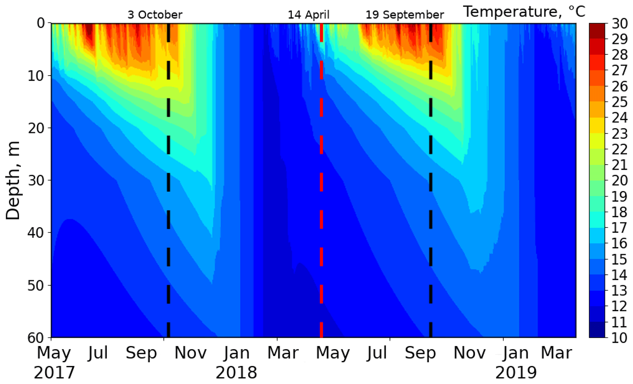
Figure 2Time–depth Hovmöller diagram of the LAKE 2.0 simulated water temperature in the Alqueva reservoir based on hourly data. Dashed lines indicate the end (black) and the beginning (red) of stratification.
The water temperature in upper layers increases up to 30 ∘C in the warm period, and in the hottest months (July–September) it reaches 25 ∘C at a 10 m depth. In the winter turnover period, the water temperature becomes uniform at depths of up to 30 m. From December, when the lake shows no temperature stratification, it gradually cools from 19 to 12 ∘C (in late February).
The temperature of water in the mixed layer (ML) is of a particular interest in many studies. LAKE 2.0 provides the water temperature at different depths, as defined in the model set-up and ML thickness, assuming that the ML temperature is constant (not including the surface skin effect). Since the vertical gradient of the measured ML temperature is not exactly constant, measurements from the sensor at a 0.5 m depth were chosen to represent the mixed layer temperature in Fig. 3. During the whole simulation period, ML depth in the reservoir was never less than 70 cm. Figure 3a shows the LAKE 2.0 simulated results in comparison with the measured values and FLake results of ML temperature. To smooth hourly fluctuations in such long-term simulation, moving average was used with 6 h period.

Figure 3(a) Time series (6 h moving average) of the Alqueva water temperature in mixed layer showing measured (black curve) and modelled results from LAKE 2.0 (red curve) and FLake (blue curve). (b) Temperature differences (6 h moving average) between observations and LAKE 2.0 (red curve) and FLake (blue curve). Dashed lines show the corresponding mean errors for LAKE 2.0 and FLake.
Differences between the two model results and the measurements (errors) are shown in Fig. 3b. In the period from March to November in both years, when the lake is stratified, the LAKE 2.0 model demonstrates better results, while during the cold periods (November–March) both models show similar error rates. The statistics of the comparison are presented in Table 2. Overall, the mean absolute errors for the whole simulation period are 1.27 ∘C for FLake and 0.74 ∘C for LAKE 2.0. Mean errors of the LAKE 2.0 and FLake models for the simulation period are 0.56 and 1.18 ∘C, respectively (shown as dashed lines in Fig. 3b), which means that both models tend to slightly overestimate the ML temperature. The LAKE 2.0 model results are better for warm periods, while FLake results are better for cold. Both models demonstrate an almost identical correlation for the selected periods.
Table 2Statistical results of mixed layer (ML) water temperature intercomparison. MAE – mean absolute error.
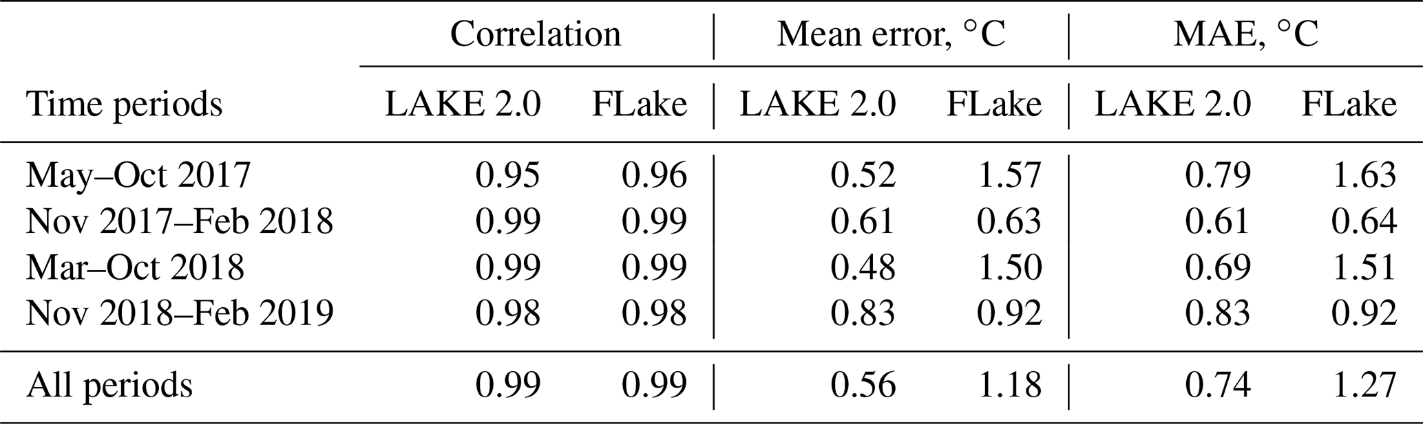
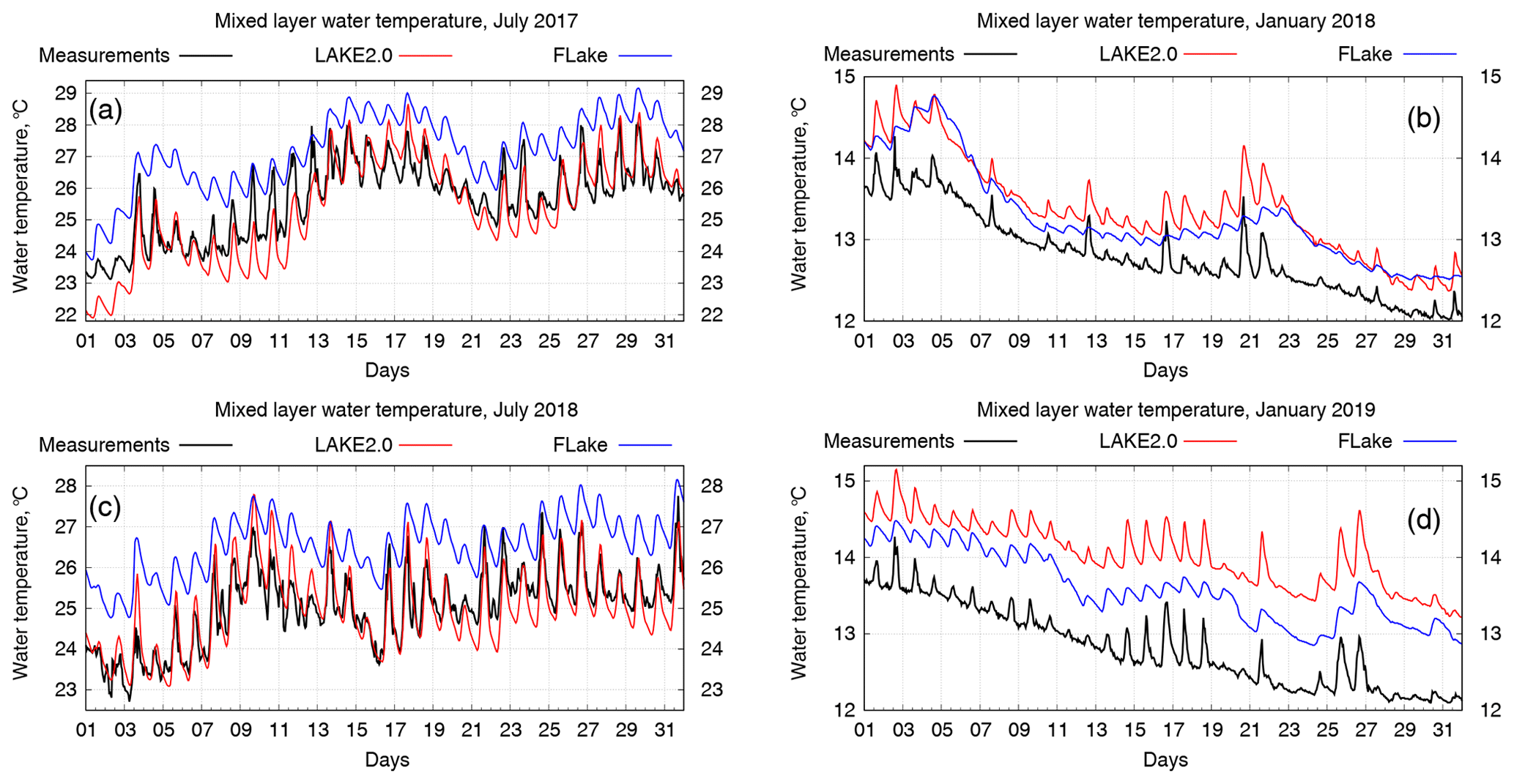
Figure 4Time series of mixed layer water temperature for July 2017 and 2018 (a and c) and January 2018 and 2019 (b and d).
For a more detailed analysis of the surface water temperature evolution, we chose four months, namely July 2017–2018 and January 2018–2019, which represent the stratified and non-stratified lake states that show the daily cycles of the ML water temperature (Fig. 4).
It is seen that the LAKE 2.0 model shows exceptionally good results in summer months (Fig. 4a; average mean errors are −0.23 and −0.04 ∘C for 2017 and 2018, respectively), while FLake provides an overestimation of 1–2∘ and an underestimation of the daily amplitude. Correlation coefficients in this case are 0.94∕0.88 (LAKE 2.0) and 0.90∕0.89 (FLake), respectively. Diurnal ML temperature variations can reach 3∘ and are generally well represented by the LAKE 2.0 model. In January the water temperature profile in the reservoir is homogeneous, the daily amplitude is not so high (Fig. 4b), and so the FLake model shows a smaller overestimation (0.95 correlation for both months and mean errors of 0.45/0.78 ∘C). The LAKE 2.0 results show a positive offset; the average mean error for January 2018 was 0.78 ∘C and the correlation was 0.97. In January 2019, the LAKE 2.0 mean error was 1.22 ∘C but, in general, the shape of the curve was similar to the measured values, and the daily variations in temperature were represented quite well.
Temperature distribution with depth is another significant parameter for lake thermodynamics. The LAKE 2.0 model simulates water temperature at predefined depth levels. FLake outputs include ML depth temperature, shape factor for the thermocline curve, and temperature at the bottom. Using these values it is possible to retrieve a water temperature profile. Simulation results are shown in Fig. 5 for the following cases: 15 July 2017, 15 January 2018, 15 July 2018, and 15 January 2019, each at 12:00 UTC.
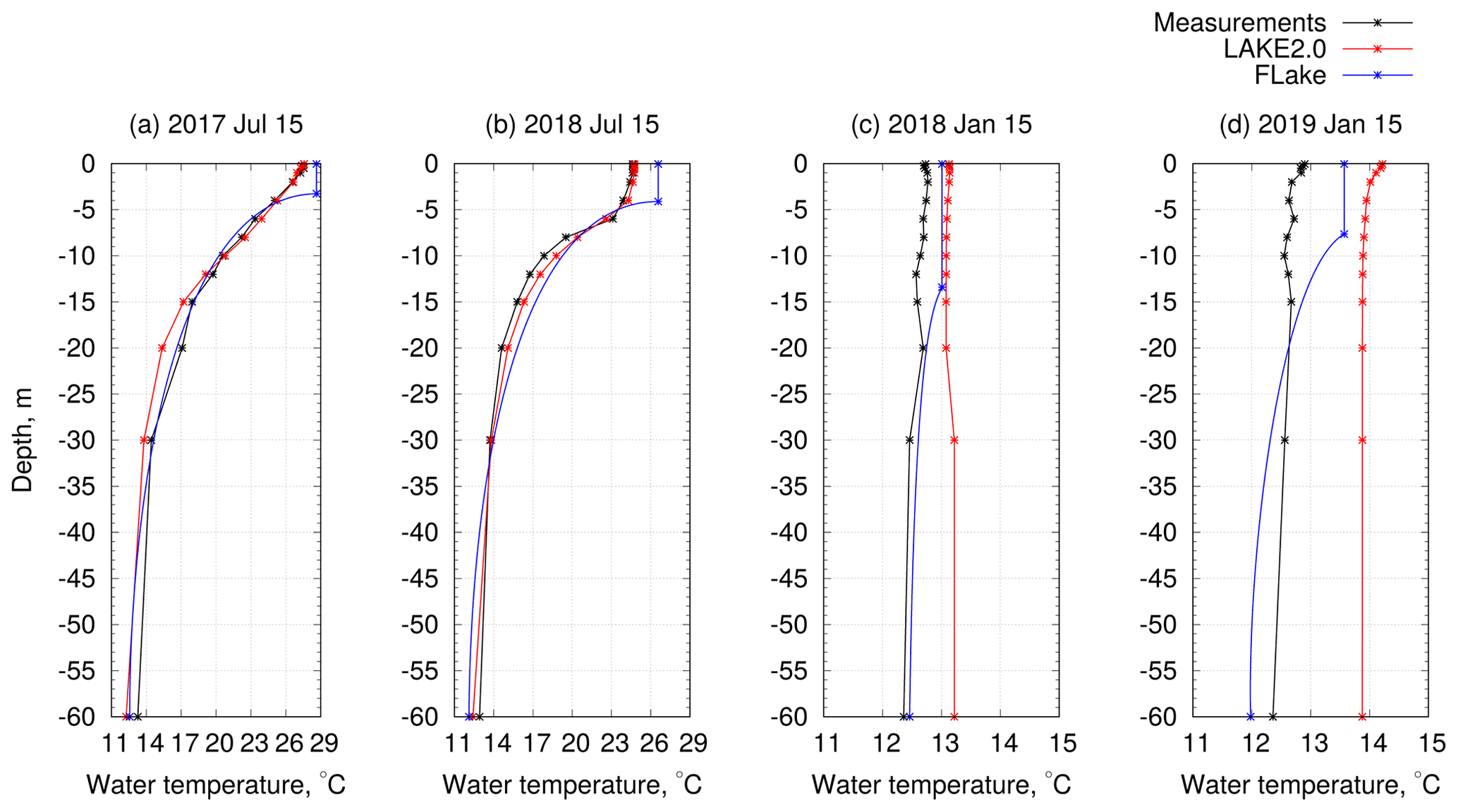
Figure 5Water temperature profiles for 15 July 2017 (a), 15 January 2018 (b), 15 July 2018 (c), and 15 January 2019 (d), each at 12:00 UTC.
Summer water temperature profiles are well represented by both models, although FLake shows an overestimation in the ML. In winter, on the other hand, LAKE 2.0 overestimates the water temperature through whole water column. Although LAKE 2.0 reproduces the short-term (daily and weekly scales) thermal evolution of the ML very well, the simulated heat content of the entire water column seemed to be higher than in reality. The errors are higher in the second year of the simulation, with the results of winter 2018–2019 exceeding 1∘. The modelled water column tends to heat slightly more than the actual water column (Fig. 5c–d). This behaviour may be due to a small misrepresentation of the energy balance at the lake surface or at the bottom and requires additional tests that could eliminate such systematic errors and improve the results, especially in cold periods.
The other important parameter, which is essentially connected with the lake's vertical thermal structure, is the depth of the mixed layer. To estimate it, we assumed that the ML ends at a point of half of the maximum temperature gradient (but not less than 0.5 ∘C). Such a criterion was used for observed data and LAKE 2.0 results. In FLake, the ML depth is a major diagnostic variable, updated at each time step using a sophisticated formulation, that treats both the convective and stable regimes (see Mironov et al., 2010). The time series of the ML depth for the 2017 and 2018 Alqueva reservoir's stratification periods are shown in Fig. 6.
The curves of the ML depth calculated from measurements and LAKE 2.0 results coincide quite well. However, since the simulated water temperature profiles are more smooth, the LAKE 2.0 ML depth has more “downward” peaks in the figure. Although FLake tends to underestimate the ML depth, the general pattern of it correlates with the measurements.
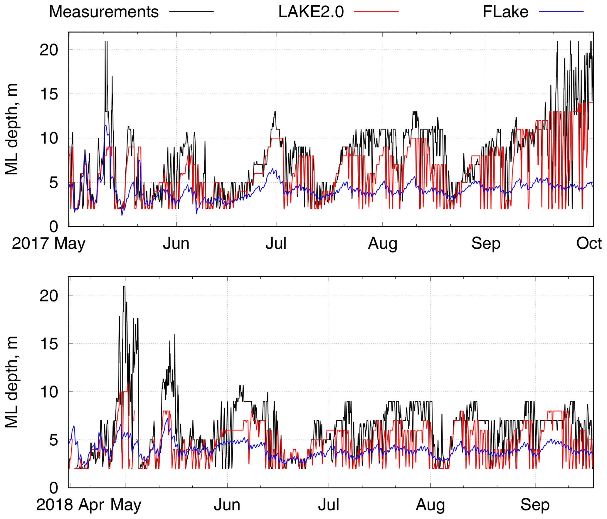
Figure 6Evolution of mixed layer (ML) depth during stratification periods (with 6 h moving average).
3.2 Heat fluxes
Sensible and latent heat fluxes play an important role in lake–atmosphere interaction, determining the rates of heat accumulation by water bodies or evaporation from the surface and consequently having effects on the local climate and on the establishment of thermal circulations (see for example Iakunin et al., 2018). The LAKE 2.0 model (and FLake) is capable of calculating heat fluxes, and Fig. 7 shows the daily averaged results of the simulation of these variables.
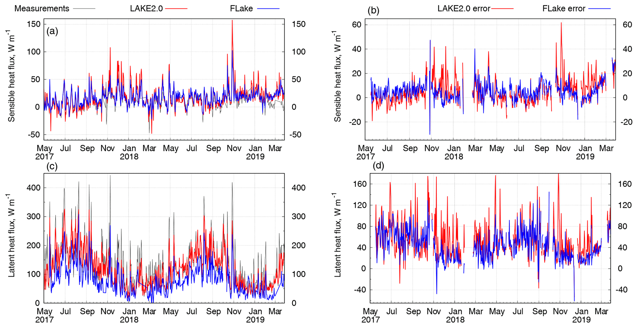
Figure 7Daily averaged sensible (a) and latent (c) heat fluxes with corresponding errors (b and d). Black curve represents the measured values, the red curve shows LAKE 2.0 results, and the blue curve shows FLAKE results.
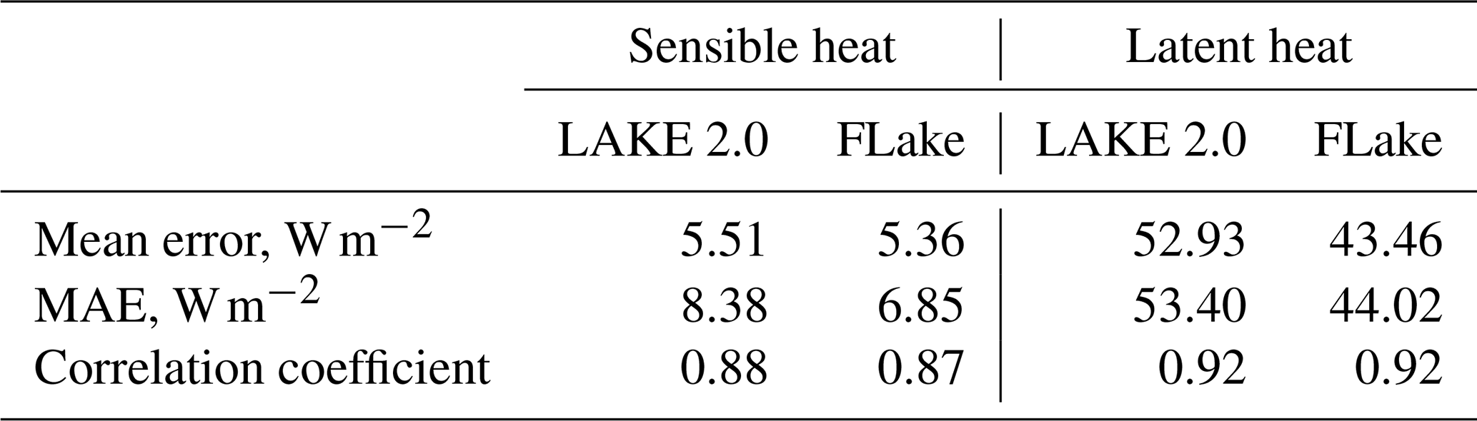
Sensible heat flux is well represented by both models (Fig. 7a–b), which is supported by low mean errors (see Table 3) and a high correlation coefficient. Latent heat flux, however, is overestimated by the LAKE 2.0 and FLake models (by 53–43 W m−2), although both models demonstrate a high correlation (0.92) with the measurements.
In terms of latent heat fluxes the LAKE 2.0 model's results are worse than the FLake's when compared to the eddy-covariance (EC) measurements. However, it should be noted that several studies have indicated that the EC systems tend to underestimate the heat fluxes (e.g. Twine et al., 2000). Recent works showed comparable differences between the FLake and the LAKE 2.0 models and EC measurements over lakes (Stepanenko et al., 2014; Heiskanen et al., 2015) in which the relative differences of about 35 % were noticed. The differences between model and EC observations can also come from model errors due to the fact that the Alqueva reservoir is an open lake with a continuous inflow and outflow of the Guadiana River. The horizontal flows, not represented in the 1D vertical models, can add or remove energy from the water body. Also, the water level in the Alqueva reservoir changes significantly during the year due to drought periods and discharges through the dam. It decreased to 7 m in 2018, which corresponds to the loss of 35 % of total volume of water. The models cannot take into an account those changes while they could be a major source of errors in heat flux computations.
Table 3Sensible and latent heat flux errors and correlation coefficients.
3.3 Dissolved carbon dioxide
The diffusion of CO2 from the atmosphere to water and its further dissociation are of major importance to photosynthetic organisms which depend on the availability of inorganic carbon (Wetzel, 1983). Dissolved inorganic carbon constituents also influence water quality properties such as acidity, hardness, and related characteristics.
The solubility of CO2 in water depends on several factors such as pH, water temperature, etc. Observations indicate that pH may vary from 8.8 at the surface level to 7.4 at the bottom, while in the model it is a constant parameter value which was set to a value of 8.48, which corresponded to the mean pH value during the simulation period. Figure 8 reveals the dynamics of CO2 concentrations in water in the first months of the ALOP field campaign in comparison with LAKE 2.0 simulated results.
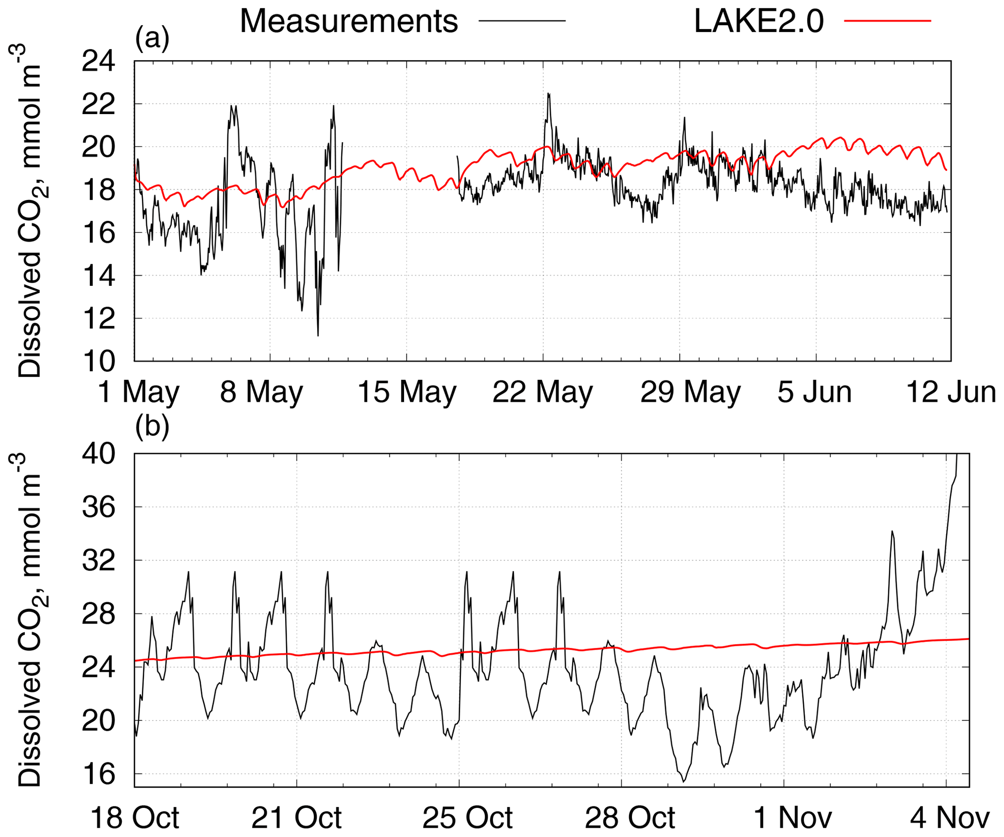
In general, the LAKE 2.0 values are smoother than the observations as the model does not react to the changes in CO2 as fast, but the mean values are well represented. On 20–26 May and at the beginning of June (subplots in Fig. 8a), daily cycles are represented quite well. In the second week of May, the CO2 probe accidentally dismounted from the platform and floated in the water, attached to the connecting cord, until the next fieldwork trip (17 May). On 12 June the probe failed, and it was dismounted and removed from the Montante platform. Later, on 18 October, the probe was mounted on the platform again and it was working in a test mode for three weeks (Fig. 8b). In this period, LAKE 2.0 simulated values of CO2 do not show much daily variation and have an increasing trend due to autumn water cooling. Small daily biases in simulated values coincide with peaks in measured data. Thus, we can conclude that in long time simulations the LAKE 2.0 model represents CO2 trends quite well. The model failed to reproduce the diurnal cycle of the surface carbon dioxide concentration, which calls for inquiry of parameterizations of photosynthesis and respiration in the model. However, the diurnal means are well captured which is enough with respect to using the model in climate applications.
3.4 Dissolved oxygen
Dissolved oxygen (DO) is essential to all aerobic organisms living in lakes or reservoirs. To understand the distribution, behaviour, and growth of these organisms, it is necessary to know the solubility and dynamics of oxygen distribution in water. The rates of supply of DO from the atmosphere and from photosynthetic inputs and the hydromechanical distribution of oxygen are counterbalanced by the consumptive metabolism. The rate of oxygen utilization in relation to synthesis permits an approximate evaluation of the metabolism of the lake as a whole (Wetzel, 1983).

Figure 9Time series of dissolved O2 in water at 25 cm depth for the period 3 July 2018–29 March 2019 at the Alqueva reservoir.
The concentration of DO in the Alqueva reservoir was measured continuously on the Montante platform from 3 July 2018. A comparison of measured and model values is shown in Fig. 9. The model represents DO concentration in a realistic way during the first 2 months, until the middle of September, when a microalgal bloom occurred. It caused an intensive production of O2 in the water that cannot be represented by the LAKE 2.0, which does not have an explicit representation of algae, and the bloom does not affect atmospheric forcing. Then, until the end of October, the model showed good results, but in November the observations demonstrated a decrease in oxygen concentration, which was not followed by the model; in fact, the model predicted an increase until the beginning of February. In November, following turnover, water temperature decreases and does not change significantly with depth; under these conditions the concentration of oxygen-producing organisms decreases, and so does the DO, which falls from 8–9 to 6 mg L−1. The model does not reflect this decrease in photosynthesis but largely increases the DO concentration following the decrease in water temperature (oxygen is more soluble in colder water). When, in the middle of February, the temperature returns to a stratified regime, DO concentrations in the model and measurements coincide again.
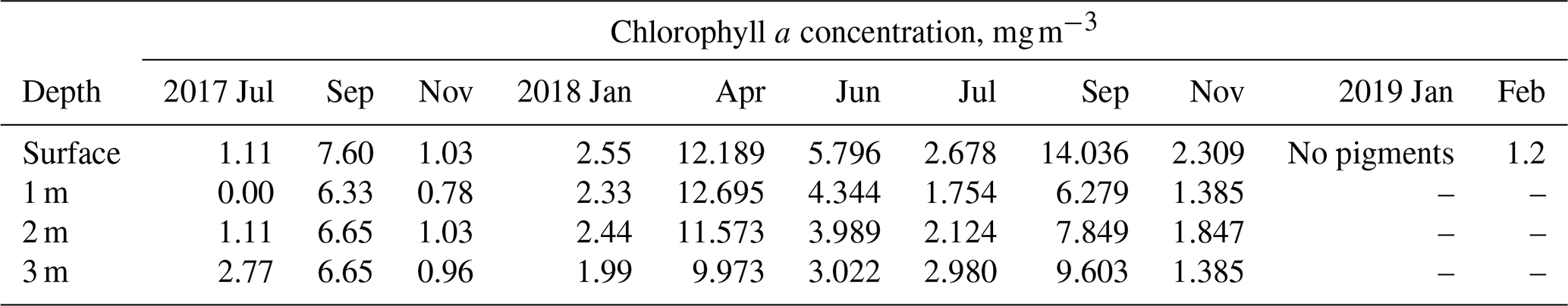
The photosynthesis rate can be linked to chlorophyll a measurements (Table 4) which were done during the fieldwork at the Alqueva reservoir. In July 2018, when DO measurements began, the concentration of chlorophyll a ranged from 1.754 to 2.98 mg m−3 in water ML (0–3 m). Furthermore, when the autumn bloom occurred in September, the chlorophyll concentration significantly increased and reached 14.036 mg L−1 at the surface and came back to values of 2.309 mg m−3 in November. The ALOP field campaign ended in December 2018, but the work on stations and the Montante platform maintenance continued, so, in January and February 2019, samples from water surface layer were taken. The sample from 15 January showed no traces of chlorophyll a in water, which is related to very low DO concentrations in this period (Fig. 9). The measurements of chlorophyll a in the water sample taken on 2 February showed the value of 1.3 mg m−3. It corresponds to the relative increase in oxygen producers in water and, hence, DO concentration.
An analysis of DO profiles (Fig. 10) shows similar results. The distribution of oxygen with depth is well represented by the model for the July and September profiles, while in December and February, with no stratification in temperature and oxygen, the LAKE 2.0 model overestimates DO up to 2.5 mg L−1. March profiles (1 and 29) show good similarities in the measured and simulated values.
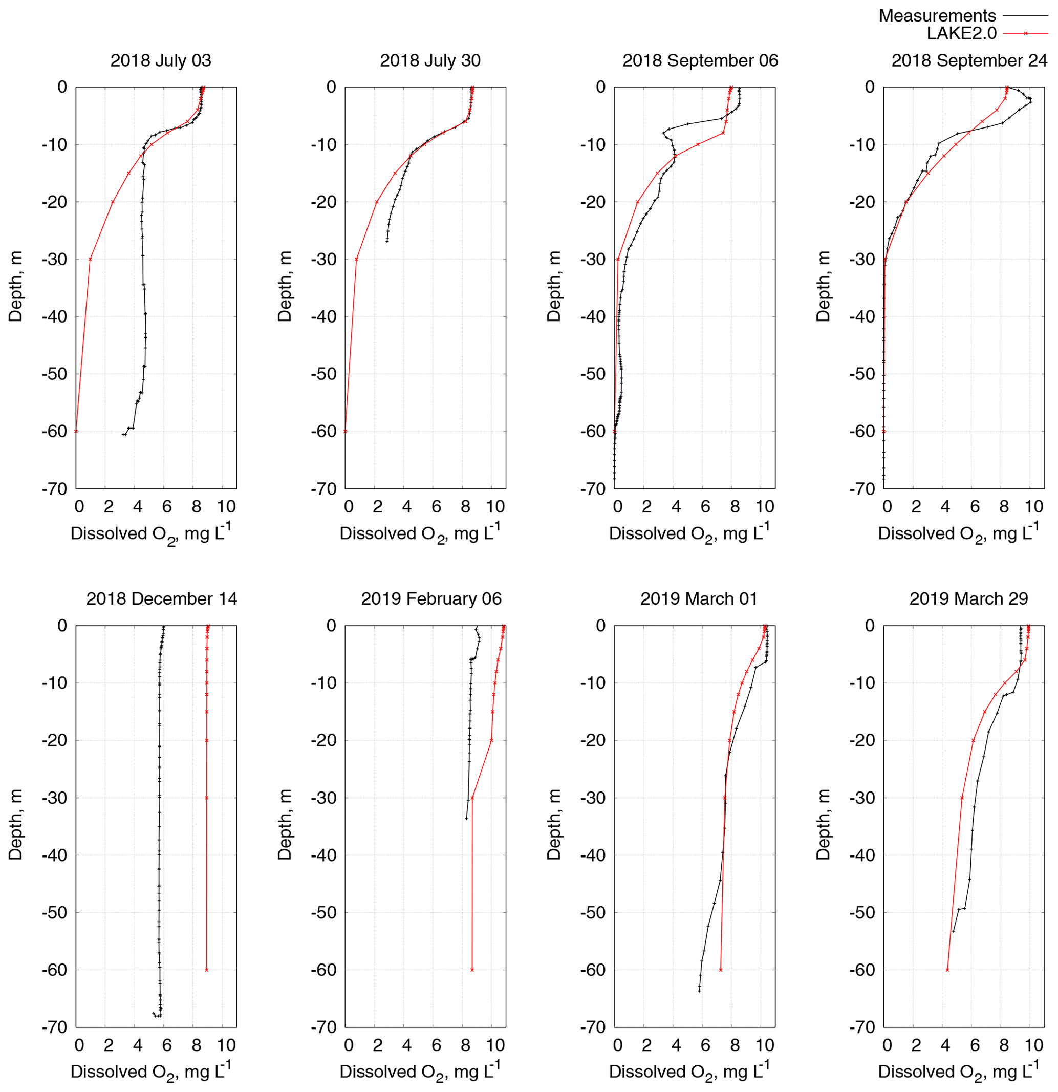
Figure 10Profiles of dissolved O2 in water measured during the field campaign (black) and model values (red).
Numerical studies of the seasonal variations in the thermal and gas regimes in the Alqueva reservoir using the LAKE 2.0 and the FLake models are presented in this work. Simulated profiles and time series of water temperature, sensible and latent heat fluxes, and concentrations of dissolved CO2 and O2 were compared with observed data. The seasonal variations in the ML water temperature are well represented by both models. Mean absolute errors are 0.74 and 1.27 ∘C for LAKE 2.0 and FLake models, respectively, and the correlation coefficients for the relationship between simulated and measured temperatures are 0.99 for both. The LAKE 2.0 model overestimates ML water temperature only by 0.5 ∘C during the warm periods (March–October), while FLake shows an overestimation of about 1.5∘. In the cold periods (November–February) both models show the same level of overestimation of ML temperatures (about 0.6–0.9 ∘C).
The model errors of the seasonal variations in sensible and latent heat fluxes are the following. Sensible heat mean absolute errors (MAEs) are 7.71 Wm−2 (LAKE 2.0) and 6.75 W m−2 (FLake). Latent heat flux results of both models in terms of MAE are worse, namely 53.99 W m−2 (LAKE 2.0) and 45.6 W m−2 (FLake). Such errors occur mainly in periods when the wind increases suddenly. Strong single high hourly wind input data cause high latent heat simulated values, which are not always confirmed by the observations.
LAKE 2.0 simulated dissolved carbon CO2 time series demonstrated a good correspondence with the observations in mean values; however, the model significantly underestimated the magnitude of the diurnal cycle. In the 18th month of the experiment (October 2018, when the probe was returned to the platform), the simulated CO2 values did not show large residuals despite the fact that the pH value remained constant during the whole simulation.
Dissolved oxygen, reproduced by the model, reveals the need to include a more complete description of the processes that regulate photosynthesis and respiration in the LAKE 2.0 model before operational use. Although measured oxygen concentrations are well simulated over short time intervals, the annual Alqueva reservoir oxygen cycle cannot be reproduced because the model does not respond to changes in the algal concentration. The winter overestimation is probably due to relatively low water temperatures. Nevertheless, the high versatility and flexibility of the LAKE 2.0 model gives good opportunities for improving the model performance, with the aim of adequate modelling of seasonal variations in the gas regime of the lake.
Performed simulations showed that the LAKE 2.0 model accurately simulates the lake's thermal regime and the heat and gas fluxes from the ML. In terms of water temperature profile, LAKE 2.0 demonstrated a better performance than the FLake model. The results are encouraging regarding the ability of the LAKE 2.0 model to represent the evolution of physicochemical profiles of lakes, and it may be used operationally in the future, coupled with weather prediction models, to forecast variables that are useful in the management of water quality and aquatic ecosystems. Similarly, the results indicate that the LAKE 2.0 model could be used in climate modelling to estimate the impacts of the climate change in the thermal and gas regimes of the lake.
The current versions of the models used in this work, and the atmospheric forcing data, can be found at https://doi.org/10.5281/zenodo.3608230 (Iakunin et al., 2020) or upon request from the corresponding author (miakunin@uevora.pt or m.yakunin89@gmail.com). The source code of the FLake model is available at (http://www.flake.igb-berlin.de/site/download, Mironov, 2008). The source code for the latest version of the LAKE 2.0 model is available at (http://tesla.parallel.ru/Viktor/LAKE/wikis/LAKE-model, Stepanenko et al., 2016).
The supplement related to this article is available online at: https://doi.org/10.5194/gmd-13-3475-2020-supplement.
MI was responsible for the numerical simulation setup, run, processing and analysis of the results. VS assisted in LAKE model setup and upgrades. RS took part in the general experiment setup and analysis of the results. MP, AP, MHN, and GR provided and processed data of observations and took part in model result analysis. All the co-authors participated in writing and editing the article.
The authors declare that they have no conflict of interest.
This work has been co-funded by the Portuguese Foundation for Science and Technology (FCT), through the project UIDB/04683/2020 of the Institute of Earth Sciences (ICT), and by the European Union through the European Regional Development Fund, included in the COMPETE 2020 (Operational Programme: “Competitiveness and Internationalization”) programme, and through the ALOP project (grant no. ALT20-03-0145-FEDER-000004). Victor Stepanenko was supported by the Russian Science Foundation (grant no. 17-17-01210) and Russia's President Grant Council (grant no. MD-1850.2020.5).
This paper was edited by Paul Ullrich and reviewed by two anonymous referees.
Adrian, R., O'Reilly, C. M., Zagarese, H., Baines, S. B., Hessen, D. O., Keller, W., Livingstone, D. M., Sommaruga, R., Straile, D., Van Donk, E., Weyhenmeyer, G. A., and Winder, M.: Lakes as sentinels of climate change, Limnol. Oceanogr., 54, 2283–2297, https://doi.org/10.4319/lo.2009.54.6_part_2.2283, 2009. a
Balsamo, G.: Interactive lakes in the Integrated Forecasting System, ECMWF Newsletter, 137, 30–34, https://doi.org/10.21957/rffv1gir, 2013. a
Bonan, G. B.: Sensitivity of a GCM Simulation to Inclusion of Inland Water Surfaces, J. Climate, 8, 2691–2704, https://doi.org/10.1175/1520-0442(1995)008<2691:SOAGST>2.0.CO;2, 1995. a, b, c
Canuto, V. M., Howard, A., Cheng, Y., and Dubovikov, M. S.: Ocean Turbulence. Part I: One-Point Closure Model-Momentum and Heat Vertical Diffusivities, J. Phys. Oceanogr., 31, 1413–1426, https://doi.org/10.1175/1520-0485(2001)031<1413:OTPIOP>2.0.CO;2, 2001. a
Dutra, E., Stepanenko, V., Balsamo, G., Viterbo, P., Miranda, P., Mironov, D., and Schaer, C.: An offline study of the impact of lakes on the performance of the ECMWF surface scheme, Boreal Environ. Res., 15, 100–112, 2010. a, b
Ekhtiari, N., Grossman-Clarke, S., Koch, H., Souza, W. M., Donner, R. V., and Volkholz, J.: Effects of the Lake Sobradinho Reservoir (Northeastern Brazil) on the Regional Climate, Climate, 5, 50, https://doi.org/10.3390/cli5030050, 2017. a
Hanson, P. C., Pollard, A. I., Bade, D. L., Predick, K., Carpenter, S. R., and Foley, J. A.: A model of carbon evasion and sedimentation in temperate lakes, Glob. Change Biol., 10, 1285–1298, https://doi.org/10.1111/j.1529-8817.2003.00805.x, 2004. a
Heiskanen, J. J., Mammarella, I., Ojala, A., Stepanenko, V., Erkkilä, K.-M., Miettinen, H., Sandström, H., Eugster, W., Leppäranta, M., Järvinen, H., Vesala, T., and Nordbo, A.: Effects of water clarity on lake stratification and lake-atmosphere heat exchange, J. Geophys. Res.-Atmos., 120, 7412–7428, https://doi.org/10.1002/2014JD022938, 2015. a, b
Hipsey, M. R., Bruce, L. C., Boon, C., Busch, B., Carey, C. C., Hamilton, D. P., Hanson, P. C., Read, J. S., de Sousa, E., Weber, M., and Winslow, L. A.: A General Lake Model (GLM 3.0) for linking with high-frequency sensor data from the Global Lake Ecological Observatory Network (GLEON), Geosci. Model Dev., 12, 473–523, https://doi.org/10.5194/gmd-12-473-2019, 2019. a
Hondzo, M. and Stefan, H. G.: Lake Water Temperature Simulation Model, J. Hydraul. Eng., 119, 1251–1273, https://doi.org/10.1061/(ASCE)0733-9429(1993)119:11(1251), 1993. a
Iakunin, M., Salgado, R., and Potes, M.: Breeze effects at a large artificial lake: summer case study, Hydrol. Earth Syst. Sci., 22, 5191–5210, https://doi.org/10.5194/hess-22-5191-2018, 2018. a, b, c, d
Iakunin, M., Stepanenko, V., Salgado, R., Potes, M., Rodrigues, G., Penha, A., and Novais, M. H.: Atmospheric forcing dataset for Numerical study of the seasonal thermal and gas regimes of the large artificial lake in Western Europe using LAKE2.0 [Data set], Zenodo, https://doi.org/10.5281/zenodo.3608230, 2020. a
Imberger, J. and Patterson, J. C.: A dynamic reservoir simulation model-DYRESM: 5, in: Transport Models for Inland and Coastal Waters, edited by: Fischer, H. B., Academic Press, New York, 310–361, 1981. a
Le Moigne, P., Colin, J., and Decharme, B.: Impact of lake surface temperatures simulated by the FLake scheme in the CNRM-CM5 climate model, Tellus A, 68, 31274, https://doi.org/10.3402/tellusa.v68.31274, 2016. a, b
Lopes, F., Silva, H. G., Salgado, R., Potes, M., Nicoll, K. A., and Harrison, R. G.: Atmospheric electrical field measurements near a fresh water reservoir and the formation of the lake breeze, Tellus A, 68, 31592, https://doi.org/10.3402/tellusa.v68.31592, 2016. a
Mironov, D.: Parameterization of lakes in numerical weather prediction. Description of a lake model, COSMO Technical Report, Deutscher Wetterdienst, 11, 41 pp., 2008. a
Mironov, D., Rontu, L., Kourzeneva, E., and Terzhevik, A.: Towards improved representation of lakes in numerical weather prediction and climate models: Introduction to the special issue of Boreal Environment Research, Boreal Environ. Res., 15, 97–99, 2010. a, b, c
Monin, A. S. and Obukhov, A. M.: Basic regularity in turbulent mixing in the surface layer of the atmosphere, U.S.S.R. Academy of Science, Works of the Geophysical Institute, 151, 163–187, 1954. a
Novais, M. H., Penha, A., Morales, E., Potes, M., Salgado, R., and Morais, M.: Vertical distribution of benthic diatoms in a large reservoir (Alqueva, Southern Portugal) during thermal stratification, Sci. Total Environ., 659, 1242–1255, https://doi.org/10.1016/j.scitotenv.2018.12.251, 2018. a
Patterson, J. C., Hamblin, P. F., and Imberger, J.: Classification and dynamic simulation of the vertical density structure of lakes, Limnol. Oceanogr., 29, 845–861, https://doi.org/10.4319/lo.1984.29.4.0845, 1984. a
Penha, A. M., Chambel, A., Murteira, M., and Morais, M.: Influence of different land uses on groundwater quality in southern Portugal, Environ. Earth Sci., 75, 622, https://doi.org/10.1007/s12665-015-5038-7, 2016. a, b
Pereira, H., Figueira, J. R., and Marques, R. C.: Multiobjective Irrigation Model: Alqueva River Basin Application, J. Irrig. Drain. E., 145, 05019006, https://doi.org/10.1061/(ASCE)IR.1943-4774.0001396, 2019. a
Policarpo, C., Salgado, R., and Costa, M. J.: Numerical Simulations of Fog Events in Southern Portugal, Adv. Meteorol., 2017, 1276784, https://doi.org/10.1155/2017/1276784, 2017. a
Potes, M., Costa, M. J., da Silva, J. C. B., Silva, A. M., and Morais, M.: Remote sensing of water quality parameters over Alqueva Reservoir in the south of Portugal, Int. J. Remote Sens., 32, 3373–3388, https://doi.org/10.1080/01431161003747513, 2011. a
Potes, M., Costa, M. J., and Salgado, R.: Satellite remote sensing of water turbidity in Alqueva reservoir and implications on lake modelling, Hydrol. Earth Syst. Sci., 16, 1623–1633, https://doi.org/10.5194/hess-16-1623-2012, 2012. a, b, c
Potes, M., Salgado, R., Costa, M. J., Morais, M., Bortoli, D., Kostadinov, I., and Mammarella, I.: Lake–atmosphere interactions at Alqueva reservoir: a case study in the summer of 2014, Tellus A, 69, 1272787, https://doi.org/10.1080/16000870.2016.1272787, 2017. a
Potes, M., Rodrigues, G., Penha, A. M., Novais, M. H., Costa, M. J., Salgado, R., and Morais, M. M.: Use of Sentinel 2 – MSI for water quality monitoring at Alqueva reservoir, Portugal, Proc. IAHS, 380, 73–79, https://doi.org/10.5194/piahs-380-73-2018, 2018. a
Salgado, R. and Le Moigne, P.: Coupling of the FLake model to the Surfex externalized surface model, Boreal Environ. Res., 15, 231–244, 2010. a, b, c, d
Samuelsson, P., Kourzeneva, E., and Mironov, D.: The impact of lakes on the European climate as simulated by a regional climate model, Boreal Environ. Res., 15, 113–129, available at: http://www.borenv.net/BER/pdfs/ber15/ber15-113.pdf (last access: 1 August 2020), 2010. a, b
Silva, A., De Lima, I., Santo, F., and Pires, V.: Assessing changes in drought and wetness episodes in drainage basins using the Standardized Precipitation Index, Bodenkultur, 65, 31–37, 2014. a
Stefan, H. and Fang, X.: Dissolved Oxygen Model for Regional Lake Analysis, Ecol. Model., 71, 37–68, https://doi.org/10.1016/0304-3800(94)90075-2, 1994. a
Stepanenko, V., Jöhnk, K. D., Machulskaya, E., Perroud, M., Subin, Z., Nordbo, A., Mammarella, I., and Mironov, D.: Simulation of surface energy fluxes and stratification of a small boreal lake by a set of one-dimensional models, Tellus A, 66, 21389, https://doi.org/10.3402/tellusa.v66.21389, 2014. a
Stepanenko, V., Mammarella, I., Ojala, A., Miettinen, H., Lykosov, V., and Vesala, T.: LAKE 2.0: a model for temperature, methane, carbon dioxide and oxygen dynamics in lakes, Geosci. Model Dev., 9, 1977–2006, https://doi.org/10.5194/gmd-9-1977-2016, 2016. a, b, c
Stepanenko, V. M., Repina, I. A., Ganbat, G., and Davaa, G.: Numerical Simulation of Ice Cover of Saline Lakes, Izvestiya, Atmos. Ocean. Phys., 55, 129–138, https://doi.org/10.1134/S0001433819010092, 2019. a
Su, D., Hu, X., Wen, L., Lyu, S., Gao, X., Zhao, L., Li, Z., Du, J., and Kirillin, G.: Numerical study on the response of the largest lake in China to climate change, Hydrol. Earth Syst. Sci., 23, 2093–2109, https://doi.org/10.5194/hess-23-2093-2019, 2019. a, b
Subin, Z. M., Riley, W. J., and Mironov, D.: An improved lake model for climate simulations: Model structure, evaluation, and sensitivity analyses in CESM1, J. Adv. Model. Earth Sy., 4, M02001, https://doi.org/10.1029/2011MS000072, 2012. a
Thiery, W., Martynov, A., Darchambeau, F., Descy, J.-P., Plisnier, P.-D., Sushama, L., and van Lipzig, N. P. M.: Understanding the performance of the FLake model over two African Great Lakes, Geosci. Model Dev., 7, 317–337, https://doi.org/10.5194/gmd-7-317-2014, 2014. a
Tomaz, A., Patanita, M., Guerreiro, I., Boteta, L., and Palma, J. F.: Water use and productivity of maize-based cropping systems in the Alqueva Region (Portugal), Cereal Res. Commun., 45, 1–11, https://doi.org/10.1556/0806.45.2017.036, 2017. a
Twine, T., Kustas, W. P., Norman, J., Cook, D., Houser, P., Teyers, T. P., Prueger, J. H., Starks, P., and Wesely, M.: Correcting Eddy-Covariance Flux Underestimates over a Grassland, Agr. Forest Meteorol., 103, https://doi.org/10.1016/S0168-1923(00)00123-4, 2000. a
Walter, K. M., Smith, L. C., and Chapin, F. S.: Methane bubbling from northern lakes: present and future contributions to the global methane budget, Philos. T. Roy. Soc. A, 365, 1657–1676, https://doi.org/10.1098/rsta.2007.2036, 2007. a
Wetzel, R. G.: Limnology, Saunders College Publishing, 2nd Edn., 1983. a, b, c