An ensemble Kalman filter data assimilation system for the whole neutral atmosphere

A data assimilation system with a four-dimensional local ensemble transform Kalman filter (4D-LETKF) is developed to make a new analysis dataset for the atmosphere up to the lower thermosphere using the Japanese Atmospherics General Circulation model for Upper Atmosphere Research. The time period from 10 January to 20 February 2017, when an international radar network observation campaign was performed, is focused on. The model resolution is T42L124, which can resolve phenomena at synoptic and larger scales. A conventional observation dataset provided by the National Centers for Environmental Prediction, PREPBUFR, and satellite temperature data from the Aura Microwave Limb Sounder (MLS) for the stratosphere and mesosphere are assimilated. First, the performance of the forecast model is improved by modifying the vertical profile of the horizontal diffusion coefficient and modifying the source intensity in the non-orographic gravity wave parameterization by comparing it with radar wind observations in the mesosphere. Second, the MLS observational bias is estimated as a function of the month and latitude and removed before the data assimilation. Third, data assimilation parameters, such as the degree of gross error check, localization length, inflation factor, and assimilation window, are optimized based on a series of sensitivity tests. The effect of increasing the ensemble member size is also examined. The obtained global data are evaluated by comparison with the Modern-Era Retrospective analysis for Research and Applications version 2 (MERRA-2) reanalysis data covering pressure levels up to 0.1 hPa and by the radar mesospheric observations, which are not assimilated.

1 Introduction

It is well known that the earth's climate is remotely coupled: for example, when El Niño occurs, convective activity in the tropics strongly affects midlatitude climate with the appearance of the Pacific–North American pattern (Horel and Wallace, 1981). Convective activity in maritime continents also modulates midlatitude climates by generating the Pacific–Japan pattern (Nitta, 1987). Most of these climate couplings between the tropics and midlatitude regions are caused by the horizontal propagation of stationary Rossby waves (Holton and Hakim, 2013). Teleconnection through stratospheric processes has also been known. For example, the sea-level pressure in the Arctic rises during El Niño. It was shown that this teleconnection occurs by modulation of planetary wave intensity and propagation in the stratosphere (Cagnazzo and Manzini, 2009). It is also well known that the occurrence frequency of stratospheric sudden warming (SSW), which exerts a strong influence on the Arctic oscillation of sea-level pressure (Baldwin and Dunkerton, 2001), is high during the easterly phase of the quasi-biennial oscillation (QBO) in the equatorial stratosphere (Holton and Tan, 1980). This is also due to the modulation of the propagation of planetary waves in the stratosphere. Thus, the stratosphere is an important area that brings about the remote coupling of climate.

Recently, the presence of interhemispheric coupling through the mesosphere has been reported as well. When the temperature in the polar winter stratosphere is high, the temperature in the polar summer upper mesosphere is also high, with a slight delay (Karlsson et al., 2009). This coupling is clear for at least a 1-month average (Gumbel and Karlsson, 2011). The interhemispheric coupling, which is initiated by SSW in the winter hemisphere, occurs at shorter timescales (Körnich and Becker, 2010). When SSW occurs in association with the breaking of strong planetary waves originating from the troposphere, the westerly wind of the polar night jet significantly weakens or, in strong cases, even turns easterly. The critical-level filtering of the gravity waves toward the mesosphere is then modulated, and the gravity wave forcing that drives the mesospheric meridional circulation with an upward (downward) branch on the equatorial (polar) side becomes weak. Thus, the temperature in the equatorial region increases and the poleward temperature gradient in the summer hemisphere weakens. The weak wind layer above the easterly jet in the summer hemisphere lowers so as to satisfy the thermal wind relation. The eastward gravity wave forcing region near the weak wind layer also descends and the upward branch of the meridional circulation, which maintains extremely low temperature in the summer polar upper mesosphere, weakens.

However, there is little observational evidence of gravity wave modulation in the mesosphere. The Interhemispheric Coupling Study by Observations and Modeling (ICSOM: http://pansy.eps.s.u-tokyo.ac.jp/icsom/, last access: 26 June 2020) is a project to understand mesospheric gravity wave modulation associated with SSWs on a global scale through a comprehensive international observation campaign with a network of mesosphere–stratosphere–troposphere (MST), meteor, and medium-frequency (MF) radars as well as complementary optical and satellite-borne instruments. Since 2016, four campaigns have been successfully performed.

In the ICSOM project, we are also proceeding with a model study using a gravity-wave-permitting high-top general atmospheric circulation model (GCM) that covers the entire troposphere and middle atmosphere (up to the lower thermosphere) simultaneously. However, this is not easy because the GCMs including the entire middle atmosphere are not yet sufficiently mature even for relatively low resolutions that do not allow explicit gravity wave simulation (e.g., Smith et al., 2017). Therefore, verification of the GCMs by high-resolution observations is necessary. In the ICSOM project, by validating the high-top GCM using data from the comprehensive international radar observation campaigns, it is expected to reproduce high-resolution global data with high reliability. Using these global data, we plan to confirm the regional representation of gravity wave characteristics detected by each radar and deepen the understanding of interhemispheric coupling quantitatively with a resolution of gravity wave scales.

Gravity wave simulation research using high-resolution GCMs has been performed in the past (e.g., Hamilton et al., 1999; Sato et al., 1999, 2009, 2012; Watanabe et al., 2008; Holt et al., 2016). However, reproducing gravity wave fields in the global atmosphere at a specific date and time requires significant effort (Eckermann et al., 2018; Becker et al., 2004). Data assimilation up to the scale of gravity waves is ideal to create global high-resolution grid data sequentially. However, current data assimilation schemes work well for geostrophic motions such as Rossby waves but not necessarily for ageostrophic motions such as gravity waves. Recent studies (Jewtoukoff, et al., 2015; Ehard et al., 2018) reported that gravity waves observed in the European Center for Medium-Range Weather Forecasts (ECMWF) operational data are partly realistic in the lower and middle stratosphere, but more validation with observation data is necessary. It has also been shown that the difference in horizontal winds between reanalysis datasets is quite large in the equatorial region where the Coriolis parameter becomes zero (Kawatani et al., 2016). The reasons for this problem may be the insufficient maturity of the models to accurately express ageostrophic motions and/or the shortage of observation data, including gravity waves, to be assimilated.

Data assimilation for the mesosphere is particularly not easy, partly because the energy ratio of Rossby waves and gravity waves is reversed there (Shepherd et al., 2000) and partly because observational data for the mesosphere are significantly limited compared to those for the lower atmosphere. In addition, it has been shown that, in the upper stratosphere and the mesosphere, Rossby waves are generated in situ due to baroclinic–barotropic instability caused by wave forcing associated with breaking or critical-level absorption of gravity waves propagating from the troposphere (Watanabe et al., 2009; Ern et al., 2013; Sato and Nomoto, 2015; Sato et al., 2018). It has been found that gravity waves are spontaneously generated in the middle atmosphere from the imbalance of the polar night jet (Sato and Yoshiki, 2008; Snyder et al., 2007; Shibuya et al., 2017), from an imbalance caused by the wave forcing due to primary gravity waves (Vadas and Becker, 2018; Hayashi and Sato, 2018), and also by shear instability caused by primary gravity wave forcing (Yasui et al., 2018). The Rossby wave generation in the middle atmosphere due to primary gravity wave forcing is regarded as a compensation problem, which makes it difficult to understand the change in the Brewer–Dobson circulation in terms of the relative roles of Rossby waves and gravity waves for climate projection with the models (Cohen et al., 2013). However, these instabilities and the in situ generation of waves in the middle atmosphere could significantly affect the momentum and energy budget in the middle atmosphere and above (Sato et al., 2018; Becker, 2017). Hence, it is necessary to understand the roles of these waves as accurately as possible based on credible, high-resolution model simulations validated by high-resolution observations.

In view of the situation described above, the following method may be one of the best existing ways to create high-resolution data for the entire middle atmosphere including gravity waves to understand the teleconnection through the mesosphere. First, a data assimilation is performed using a high-top but relatively low-resolution model to create grid data for the real atmosphere from the ground to the lower thermosphere including only larger-scale phenomena such as Rossby waves. Second, the analysis data obtained by the assimilation are used as initial values for a free run of high-resolution GCMs to simulate gravity waves. Eckermann et al. (2018) and Becker and Vadas (2018) have performed pioneering studies on the effectiveness of such free runs.

Reanalysis data over a long time period are produced using modern data assimilation schemes and released by meteorological organizations for climate analysis. These include the following: the ECMWF interim reanalysis (ERA-Interim; Dee et al., 2011) and the fifth reanalysis (ERA5; Hersbach et al., 2018) produced by a four-dimensional (4D) variational assimilation scheme (Var); MERRA (Rienecker et al., 2011) and the following version 2 (MERRA-2; Gelaro et al., 2017) by the National Aeronautics and Space Administration (NASA) by a three-dimensional Var (3D-Var); the National Centers for Environmental Prediction (NCEP) Climate Forecast System Reanalysis (CFSR; Saha et al., 2010) and the Climate Forecast System version 2 (CFSv2; Saha et al., 2014); and the Japanese 55-year reanalysis (JRA-55; Kobayashi et al., 2015) by a 4D-Var. ERA-Interim and JRA-55 cover up to a pressure of 0.1 hPa, NCEP/CFSR and NCEP/CFSv2 up to 0.266 hPa, and MERRA, MERRA-2, and ERA5 up to 0.1 hPa. However, global data for the middle and upper mesosphere to the lower thermosphere are not created regularly. As stated above, considering the importance of ageostrophic motions in the mesosphere and lower thermosphere (MLT), the data assimilation used for such meteorological organizations may not work very well for the middle stratosphere and above (Polavarapu et al., 2005). Therefore, in recent years, significant efforts have been made to assimilate data using GCMs that include the MLT region. Currently, the data available for studying the MLT region come from the Aura Microwave Limb Sounder (Aura MLS; beginning in 2004), Thermosphere Ionosphere Mesosphere Energetics and Dynamics (TIMED) Sounding of the Atmosphere using Broadband Emission Radiometry (SABER; beginning in 2002), and the Defense Meteorological Satellite Program (DMSP) Special Sensor Microwave Imager/Sounder (SSMIS; Swadley et al., 2008).

Global data for the atmosphere including the MLT region are valuable from the following viewpoints. First, they can improve prediction of the polar stratosphere (e.g., Hoppel et al., 2008, 2013; Polavarapu et al., 2005). It seems that anomalies in the MLT region start about 1 week earlier than stratospheric anomalies such as SSWs, propagating down to the troposphere. Thus, better understanding the MLT physics and chemistry has the potential to improve long-range weather forecasts. Second, it is possible to quantitatively understand the transport of minor species from the MLT region (e.g., Hoppel et al., 2008; Polavarapu et al., 2005). For example, high-energy particles originating from the upper atmosphere contribute to the production of NO_x, which modulates the ozone chemistry in the stratosphere. Thus, the quantitative evaluation of the transport of such species is important for the prediction of the ozone layer. Third, they contribute to space-weather prediction, particularly for the prediction of the near-space environment (e.g., Hoppel et al., 2013). Atmospheric waves excited in the lower and middle atmosphere, including gravity waves, Rossby waves, and tides, are main drivers of the general circulation in the height range of 100–150 km in the lower thermosphere (e.g., Akmaev, 2011; Miyoshi and Yigit, 2019). Thus, it is important to examine the properties of these waves in the mesosphere. Last but not least, it is interesting to understand middle atmosphere processes as a pure science (e.g., Hoppel et al., 2008).

The first attempt to create analysis data for the whole middle atmosphere using data assimilation was made by a Canadian group. They employed 3D-Var using the Canadian Middle Atmosphere Model (CMAM) with full interactive chemistry and nonlocal thermodynamic equilibrium (non-LTE) radiation (Polavarapu et al., 2005; Nezlin et al., 2009). The assimilation of the data in the troposphere and stratosphere has been shown to improve the analysis of large-scale phenomena (zonal wavenumber s<10) in the mesosphere (Nezlin et al., 2009). The daily mean time series from their data assimilation are validated by radar observations (Xu et al., 2011). Sankey et al. (2007) used the CMAM to carefully discuss the effectiveness of digital filters in the data assimilation. A series of studies at the Naval Research Laboratory (NRL) is remarkable. Hoppel et al. (2008) performed the first mesospheric data assimilation at the Advanced Level Physics and High-Altitude (ALPHA) prototype of the Navy Operational Global Atmospheric Prediction System (NOGAPS) using a 3D-Var assimilation system (NAVDAS). After that, they introduced a 4D-Var to assimilate data using the NRL Navy Global Environmental Model (NAVGEM), a successor of NOGAPS (Hoppel et al., 2013). In this system, the SSMIS data were also assimilated along with the SABER and Aura MLS data. The calculation of the background error covariance matrix was accelerated by introducing ensemble forecasts, and assimilation shocks to the model were reduced by using digital filters (McCormack et al., 2017; Eckermann et al., 2018). Global data with short time intervals were made by combining model forecasts with the assimilation products, and both short-term and annual variations of diurnal migrating tides were successfully captured (McCormack et al., 2017; Dhadley et al., 2018; Eckermann et al., 2018). These assimilation data products are utilized for the study of quasi-2 d waves and 5 d waves, as well as tides (Eckermann et al., 2009, 2018; Pancheva et al., 2016), and for observation projects such as the Deep Propagating Gravity Wave Experiment (DEEPWAVE; Fritts et al., 2016). A data assimilation study using the Whole Atmosphere Community Climate Model (WACCM) at the National Center for Atmospheric Research (NCAR) has been also conducted. Pedatella et al. (2014b) applied a Data Analysis Research Testbed (DART) ensemble adjustment Kalman filter (EAKF), which is a 3D-Var combined with a statistical scheme, to the WACCM and made analysis data for the largest recorded SSW event, which occurred in 2009. They indicated that better analysis of the mesosphere requires assimilation of the mesospheric observational data. A similar discussion was made by Sassi et al. (2018) using the Specified Dynamics WACCM (SD-WACCM), in which a nudging method was implemented. The reality of the analysis highly depends on the model's performance in the MLT region. One of the critical components to determine the MLT region in the model is gravity wave parameterizations (Pedatella et al., 2014a; Smith et al., 2017). According to Pedatella et al. (2018), the analysis of the SSW in 2009 by the WACCM using DART showed that the expression of the downward transport of chemical components by the data assimilation is better than by the nudging method.

Nowadays whole-atmosphere models covering the surface to the exosphere have been developed (Akmaev, 2011). Data assimilation and data nudging studies using a whole-atmosphere model were performed focusing on the SSW in 2009. These include studies using the whole-atmosphere data assimilation system (WDAS), which includes the whole-atmosphere model and a 3D-Var analysis system (Wang et al., 2011), the Ground-to-topside model of Atmosphere and Ionosphere for Aeronomy (GAIA) with a nudging method (Jin et al., 2012), and SD-WACCM (Chandran et al., 2013; Sassi et al., 2013). Outputs from a long-term run using GAIA, which was nudged to the reanalysis data up to the lower stratosphere, were used for a momentum budget analysis in the whole middle atmosphere, and the importance of the in situ generation of gravity waves and Rossby waves in the middle atmosphere was suggested (Sato et al., 2018; Yasui et al., 2018).

Although most 4D data assimilation studies described above used 4D-Var, the method using an ensemble Kalman filter is also possible. The 4D-Var codes need to be developed for each model. In contrast, the four-dimensional local ensemble transform Kalman filter (4D-LETKF) developed by Miyoshi and Yamane (2007), which is a statistical assimilation method, is versatile and can thus be implemented in any model relatively easily. This study develops an assimilation system using the 4D-LETKF with a GCM with a top in the lower thermosphere. As the first step of the ICSOM project, we used a low-resolution version of the GCM and examined the best parameters of the assimilation system for the middle atmosphere (i.e., the atmosphere up to the turbopause, ∼ 100 km), as no studies employ the 4D-LETKF to assimilate data for such a high atmospheric region. The observation datasets used for the data assimilation are Aura MLS (v.4.2) temperature, which covers the whole stratosphere and mesosphere, and NCEP PREPBUFR, which is a standard dataset for the troposphere and lower stratosphere. The target time period is from January to February 2017, which includes the second ICSOM observation campaign. On 1 February 2017, the criteria of the major SSW were satisfied. The structure of this paper is as follows. Section 2 describes the forecast model, observation data, and data assimilation system. Section 3 presents the results of the parameter assessment. Section 4 presents the results of analysis regarding fields in the middle atmosphere in ICSOM-2 using data from the best parameter setting. Section 5 gives the summary and concluding remarks.

2 Methodology

2.1 Forecast model

We used the Japanese Atmospheric GCM for Upper Atmosphere Research (Watanabe and Miyahara, 2009) as a forecast model, which we refer to as JAGUAR in this paper. This model has a high model top of approximately 150 km and is based on the T213L256 middle atmosphere GCM developed for the Kanto project (Watanabe et al., 2008) and the Kyushu-GCM (e.g., Yoshikawa and Miyahara, 2005). This model uses important physical parameterizations for the MLT region such as radiative transfer processes, including non-LTE and solar radiative heating due to molecular oxygen and ozone. The effects of ion drag, chemical heating, dissipation heating, and molecular diffusion are also parameterized in the model. In this study, a standard-resolution JAGUAR with a triangularly truncated spectral resolution of T42 corresponding to a horizontal resolution of about 300 km (a latitudinal interval of 2.8125^∘) is used for the assimilation. The model has 124 vertical layers with a uniform vertical spacing of approximately 1 km in the middle atmosphere and 100–800 m in the troposphere (see Fig. A1 of Watanabe et al., 2015, for the vertical layers). Unlike a high-resolution JAGUAR, which resolves a certain portion of gravity waves (Watanabe and Miyahara, 2009), gravity waves are sub-grid-scale phenomena for a standard-resolution JAGUAR. For this reason, both orographic (McFarlane, 1987) and non-orographic (Hines, 1997) gravity wave parameterizations are used. The wave source distribution of non-orographic parameterization is given based on the results of a gravity-wave-resolving high-resolution GCM (Watanabe, 2008), and the intensity of the source is treated as one of the tuning parameters. Horizontal diffusion is set as an e-folding time of 0.9 d for the minimum resolved wave length in the troposphere and stratosphere, and it exponentially increases with increasing height over the MLT region. In this study, the vertical profile of horizontal diffusion above the stratopause is also treated as one of the tuning parameters. The monthly ozone mixing ratio from United Kingdom Universities Global Atmospheric Modeling Programme (UGAMP; Li and Shine, 1999) and monthly sea surface temperature and sea ice concentration from the Met Office Hadley Centre sea ice and sea surface temperature dataset (HadISST; Rayner et al., 2003) are linearly interpolated in time and used as boundary conditions.

2.2 Measurements used in the assimilation

2.2.1 PREPBUFR

Observation data used for the assimilation include the PREPBUFR global observation dataset compiled by the National Centers for Environmental Prediction and archived at the University Corporation for Atmospheric Research (https://rda.ucar.edu/datasets/ds337.0/, last access: 26 June 2020), which includes surface pressure as a function of longitude and latitude, as well as temperature, wind, and humidity as functions of longitude, latitude, and pressure (or height) from radiosondes, aircrafts, wind profilers, and satellites. Ground-based observations are mainly distributed in the height range from the ground to the lower stratosphere, and approximately 70 % of the data are taken at stations located in the Northern Hemisphere. Since May 1997, daily data have been uploaded with a delay of several days. The number of data points per one assimilation step (every 6 h) is 1000–20 000 for balloon-borne radiosonde measurements, ∼ 1000 for aircraft measurements, ∼ 40 000 for satellite wind measurements, ∼ 10 000 for meteorological radar measurements, ∼ 50 000 for measurements at the ground, and ∼ 500 000 for sea scatterometer measurements.

The observation errors provided in the PREPBUFR dataset as a function of the type of measurements and altitude¹ were used in the data assimilation. For example, the observation errors in radiosonde temperature data are 1.2 K at 1000 hPa, 0.8 K at 100 hPa, and 1.5 K at 10 hPa. The horizontal resolution of the GCM used in this study is not sufficient to represent the fine structure captured by these observations. Representativeness errors, which come from the difference in resolutions between individual measurements and the model, could degrade the data assimilation performance. If representation errors are random and large numbers of observations are assimilated, their impact could be negligible. Because substantial numbers of observations are available within a model grid cell in a data assimilation cycle in our analysis, the observation data were thinned before assimilation to reduce the computational cost of the data assimilation analysis. Original data from aircraft and satellite winds are trimmed by taking one of every four consecutive data points. Radiosonde data at the standard pressure levels of 1000, 925, 850, 700, 500, 400, 300, 250, 200, 150, 100, 70, 50, and 10 hPa were used for the data assimilation. These settings are the same as the ALERA2 (Enomoto et al., 2013)

2.2.2 Aura MLS

The MLS instrument onboard the Aura satellite was launched in 2004. The satellite takes the polar orbit 14 times a day. Vertical profiles of several atmospheric parameters are retrieved from a limb sounding of the thermal emissions of the atmosphere. We used temperature data (v.4.2) retrieved from the radiation of oxygen (O₂; 118 GHz) and the oxygen isotope (O¹⁸O; 239 GHz) of Aura MLS (Livesey et al., 2018) for the assimilation. The data are distributed at 55 vertical layers from 261 to 0.001 hPa at ∼ 2 km intervals. The estimated retrieval errors are ∼ 0.5 K at 261–10 hPa, ∼ 1 K at 10–0.3 hPa, ∼ 2 K for 0.3–0.04 hPa, and ∼ 3 K for 0.04–0.001 hPa. For the observation operator, we included weighting functions (called “averaging kernels”) to consider the vertical sensitivity of the measurements. The weighting functions at the Equator and at 70^∘ N are available on the Aura MLS mission website (https://mls.jpl.nasa.gov/data/ak/, last access: 26 June 2020). Assuming that the measurement vertical sensitivity is invariant for a wide area, the averaging kernel for the Equator and that for 70^∘ N are respectively applied to the latitudinal range of 40^∘ S–40^∘ N and the remaining high-latitude regions (i.e., 40–90^∘ N and 40–90^∘ S).

The horizontal intervals of the Aura MLS observation data along the track, which is almost parallel to the meridional direction, are approximately 2^∘, so two or three profiles are included in the area represented by a grid point of the forecast model. Note that the horizontal intervals of the Aura MLS observation data between subsequent orbits are approximately 30^∘, which is much coarser than the model resolution. To reduce the computational cost of the data assimilation, the observations are horizontally averaged for the along-track direction to reduce the resolution comparable to the forecast model resolution before the assimilation, without considering any correlation between individual observation errors. Errors in the retrievals in some parameters can be correlated in space, but their quantitative estimates are difficult. The measurement error is used as the diagonal component of the observation error covariance matrix. Moreover, this average is effective to remove gravity waves that cannot be resolved by the current model. We have confirmed the importance of the averaging by comparing the results with and without the averaging (not shown).

It has been suggested that the Aura MLS data include observation bias (e.g., Randel et al., 2016). In this study, a bias correction is performed, and the effect of the bias correction on the analysis data is examined. In addition to the retrieval quality flag information, a gross error check was applied in the quality control to exclude observations that are far from the first guess. The best settings for the gross error check are considered to be different between the mesosphere and lower atmosphere because of the different growth rates of model error in a specific period of time (e.g., a data assimilation window). Thus, the appropriate degrees of the gross error check are also examined.

2.3 Data assimilation system

The 4D-LETKF (Miyoshi and Yamane, 2007) is used as a data assimilation method. This method is an extension of the 3D-LETKF (Hunt et al., 2007), which includes the dimension of time (4D ensemble Kalman filter; Hunt et al., 2004). The base of the program used in this study has already been applied to many types of forecast models, such as the Global Spectral Model (GSM; Miyoshi and Sato, 2007), the Atmospheric GCM for Earth Simulator (AFES; Miyoshi et al., 2007), and the Non-hydrostatic Icosahedral Atmospheric Model (NICAM; Terasaki et al., 2015).

This section introduces the formulas used in the 4D-LETKF. The analyses, forecasts, and observations are denoted by x^a, x^f, and y^o, respectively. The optimal value of x^a is derived from x^f and y^o by the following equation:

$$\begin{array}{}\text{(1)}& {\mathit{x}}^{\text{a}}={\mathit{x}}^{\text{f}}+\mathbf{K}\left({\mathit{y}}^{\text{o}}-\mathbf{H}{\mathit{x}}^{\text{f}}\right)={\mathit{x}}^{\text{f}}+\mathbf{K}\mathit{d},\end{array}$$

where K is a weighting function, $d(\equiv {\mathit{y}}^{\text{o}}-\mathbf{H}{\mathit{x}}^{\text{f}})$ is the innovation, and H is an observation operator that converts the model space variables into observational space variables. For assimilating MLS retrievals, the observation operator includes the averaging kernel and the spatial operator. The second term on the right-hand side represents data assimilation corrections (i.e., increments). Using the differences from the true value (x^t), $\mathit{\delta }{\mathit{x}}^{\text{a}}={\mathit{x}}^{\text{a}}-{\mathit{x}}^{\text{t}}$, $\mathit{\delta }{\mathit{x}}^{\text{f}}={\mathit{x}}^{\text{f}}-{\mathit{x}}^{\text{t}}$, and $\mathit{\delta }{\mathit{y}}^{\text{o}}={\mathit{y}}^{\text{o}}-\mathbf{H}{\mathit{x}}^{\text{t}}$, Eq. (1) can be rewritten as follows:

$$\begin{array}{}\text{(2)}& \mathit{\delta }{\mathit{x}}^{\text{a}}=\mathit{\delta }{\mathit{x}}^{\text{f}}+\mathbf{K}\left(\mathit{\delta }{\mathit{y}}^{\text{o}}-\mathbf{H}\mathit{\delta }{\mathit{x}}^{\text{f}}\right)=\left(\mathbf{I}-\mathbf{KH}\right)\mathit{\delta }{\mathit{x}}^{\text{f}}+\mathbf{K}\mathit{\delta }{\mathit{y}}^{\text{o}},\end{array}$$

where I is an identity matrix. The analysis error covariance is defined as

$$\begin{array}{}\text{(3)}& {\mathbf{P}}^{\text{a}}\equiv \langle \mathit{\delta }{\mathit{x}}^{\text{a}}(\mathit{\delta }{\mathit{x}}^{\text{a}}{)}^{\text{T}}\rangle =\left(\mathbf{I}-\mathbf{KH}\right){\mathbf{P}}^{\text{f}}{\left(\mathbf{I}-\mathbf{KH}\right)}^{\mathrm{T}}+{\mathbf{KRK}}^{\mathrm{T}},\end{array}$$

where P^f≡〈δx^f(δx^f)^T〉 is the forecast error covariance and R≡〈δy^o(δy^o)^T〉 is the observation error covariance. The correlation between the forecast error and the observation error is supposed to be zero (〈δx^f(δy^o)^T〉=0). The optimal x^a should minimize the summation of the analysis error covariance (tr(P^a)). This means that

$$\begin{array}{}\text{(4)}& {\displaystyle \frac{\partial }{\partial \mathbf{K}}}tr\left({\mathbf{P}}^{\text{a}}\right)=\mathrm{0}.\end{array}$$

Solving Eq. (4) with respect to the weight matrix K yields

$$\begin{array}{}\text{(5)}& \mathbf{K}={\mathbf{P}}^{\text{f}}{\mathbf{H}}^{\mathrm{T}}{\left({\mathbf{HP}}^{\text{f}}{\mathbf{H}}^{\mathrm{T}}+\mathbf{R}\right)}^{-\mathrm{1}},\end{array}$$

and the analysis x^a is derived by Eq. (1). The weight matrix K is called the “Kalman gain”. Using K, the analysis error covariance P^a is rewritten as

$$\begin{array}{}\text{(6)}& {\mathbf{P}}^{\text{a}}=\left(\mathbf{I}-\mathbf{KH}\right){\mathbf{P}}^{\text{f}},\end{array}$$

which gives the relationship $\mathbf{K}={\mathbf{P}}^{\text{a}}{\mathbf{H}}^{\mathrm{T}}{\mathbf{R}}^{-\mathrm{1}}$.

The size of P^f and P^a is the square of the degree of freedom in the model. Thus, for systems with huge degrees of freedom, such as GCMs, the calculation of P^f and P^a requires a large computational cost. This problem is avoided by replacing the forecast, analysis, and each error with the mean and variance for m members of an ensemble. This is called the ensemble Kalman filter (EnKF; Evensen, 2003). The ensemble mean $\stackrel{\mathrm{‾}}{\mathit{x}}$ and background error covariance matrix P are written as follows:

$$\begin{array}{}\text{(7)}& \stackrel{\mathrm{‾}}{\mathit{x}}={\displaystyle \frac{\mathrm{1}}{m}}\sum _{i=\mathrm{1}}^m{\mathit{x}}_i,\end{array}$$

$$\begin{array}{}\text{(8)}& \begin{array}{rl}\mathbf{P}& =\langle \mathit{\delta }\mathit{x}(\mathit{\delta }\mathit{x}{)}^{\text{T}}\rangle \approx {\displaystyle \frac{\mathrm{1}}{m-\mathrm{1}}}\sum _{i=\mathrm{1}}^m({\mathit{x}}_i-\stackrel{\mathrm{‾}}{\mathit{x}}){\left({\mathit{x}}_i-\stackrel{\mathrm{‾}}{\mathit{x}}\right)}^{\mathrm{T}}\\ & ={\displaystyle \frac{\mathrm{1}}{m-\mathrm{1}}}\sum _{i=\mathrm{1}}^m\mathit{\delta }{\mathit{x}}_i{\left(\mathit{\delta }{\mathit{x}}_i\right)}^{\mathrm{T}}.\end{array}\end{array}$$

However, with a limited number of ensembles, the forecast error tends to be underestimated in a system with a large degree of freedom. A variety of methods have been proposed to overcome this problem (e.g., Whitaker et al., 2008). In our study, the forecast ensemble perturbation (δx^f) is multiplied by the factor F, which is a little larger than 1 ($F=\mathrm{1}+\mathrm{\Delta }$; Δ is called an “inflation factor”):

$$\begin{array}{}\text{(9)}& \mathit{\delta }{\mathit{x}}_i^{\text{f}}\leftarrow \left(\mathrm{1}+\mathrm{\Delta }\right)\mathit{\delta }{\mathit{x}}_i^{\text{f}}\end{array}$$

is employed, and the Δ value is optimized.

The Kalman gain is simply written by using E, which is the root of P. Using

$$\begin{array}{}\text{(10)}& \sqrt{m-\mathrm{1}}\mathbf{E}\equiv \left[\mathit{\delta }{\mathit{x}}_{\mathrm{1}}\mathrm{|}\mathrm{\dots }\mathrm{|}\mathit{\delta }{\mathit{x}}_m\right],\end{array}$$

$$\begin{array}{}\text{(11)}& \begin{array}{rl}\mathbf{K}& ={\mathbf{P}}^{\text{f}}{\mathbf{H}}^{\mathrm{T}}{\left({\mathbf{HP}}^{\text{f}}{\mathbf{H}}^{\mathrm{T}}+\mathbf{R}\right)}^{-\mathrm{1}}\\ & ={\mathbf{E}}^{\text{f}}{\left({\mathbf{HE}}^{\text{f}}\right)}^{\mathrm{T}}{\left[{\mathbf{HE}}^{\text{f}}{\left({\mathbf{HE}}^{\text{f}}\right)}^{\mathrm{T}}+(m-\mathrm{1})\mathbf{R}\right]}^{-\mathrm{1}}\end{array}\end{array}$$

is derived. Further manipulation yields another expression of K:

$$\begin{array}{}\text{(12)}& \mathbf{K}={\mathbf{E}}^{\text{f}}{\left[(m-\mathrm{1})\mathbf{I}+{\left({\mathbf{HE}}^{\text{f}}\right)}^{\mathrm{T}}{\mathbf{R}}^{-\mathrm{1}}{\mathbf{HE}}^{\text{f}}\right]}^{-\mathrm{1}}{\left({\mathbf{HE}}^{\text{f}}\right)}^{\mathrm{T}}{\mathbf{R}}^{-\mathrm{1}}.\end{array}$$

To reduce the calculation cost, the inverse matrix of Eq. (11) or Eq. (12) with a smaller size is chosen. Usually, as the number of the ensemble is much smaller than the number of observations, Eq. (14) is used.

The LETKF treats the analysis error covariance matrix,

$$\begin{array}{}\text{(13)}& {\stackrel{\mathrm{̃}}{\mathbf{P}}}^{\text{a}}\equiv {\left[(m-\mathrm{1})\mathbf{I}+{\left({\mathbf{HE}}^{\text{f}}\right)}^{\mathrm{T}}{\mathbf{R}}^{-\mathrm{1}}{\mathbf{HE}}^{\text{f}}\right]}^{-\mathrm{1}},\end{array}$$

in the ensemble space. The relationship between this matrix in the ensemble space and the analysis error covariance matrix in the model space is expressed as ${\mathbf{P}}^{\text{a}}={\mathbf{E}}^{\text{f}}{\stackrel{\mathrm{̃}}{\mathbf{P}}}^{\text{a}}({\mathbf{E}}^{\text{f}}{)}^{\mathrm{T}}$, and ${\mathbf{E}}^{\text{a}}={\mathbf{E}}^{\text{f}}({\stackrel{\mathrm{̃}}{\mathbf{P}}}^{\text{a}}{)}^{\frac{\mathrm{1}}{\mathrm{2}}}$ is the ensemble update. In this way, the analysis ${\mathit{x}}_i^{\text{a}}$ is obtained as

$$\begin{array}{}\text{(14)}& {\mathit{x}}_i^{\text{a}}={\stackrel{\mathrm{‾}}{\mathit{x}}}^{\text{a}}+\mathit{\delta }{\mathit{x}}_i^{\text{a}}={\stackrel{\mathrm{‾}}{\mathit{x}}}^{\text{f}}+\mathit{\delta }{\mathit{x}}_i^{\text{a}}+{\mathbf{E}}^{\text{f}}{\stackrel{\mathrm{̃}}{\mathbf{P}}}^{\text{a}}{\left({\mathbf{HE}}^{\text{f}}\right)}^{\mathrm{T}}{\mathbf{R}}^{-\mathrm{1}}\mathit{d}.\end{array}$$

Using the shape of the N×m matrix, where N is the number of the variables, Eq. (14) is written as

$$\begin{array}{}\text{(15)}& \left[{\mathit{x}}_{\mathrm{1}}^{\text{a}}\mathrm{|}\mathrm{\dots }\mathrm{|}{\mathit{x}}_m^{\text{a}}\right]=\left[{\stackrel{\mathrm{‾}}{\mathit{x}}}^{\text{f}}\mathrm{|}\mathrm{\dots }\mathrm{|}{\stackrel{\mathrm{‾}}{\mathit{x}}}^{\text{f}}\right]+{\mathbf{E}}^{\text{f}}\mathbf{W},\end{array}$$

where

$$\begin{array}{}\text{(16)}& \mathbf{W}=({\stackrel{\mathrm{̃}}{\mathbf{P}}}^{\text{a}}{)}^{\frac{\mathrm{1}}{\mathrm{2}}}+\left[{\stackrel{\mathrm{̃}}{\mathbf{P}}}^{\text{a}}{\left({\mathbf{HE}}^{\text{f}}\right)}^{\mathrm{T}}{\mathbf{R}}^{-\mathrm{1}}\mathit{d}\mathrm{|}\mathrm{\cdots }\mathrm{|}{\stackrel{\mathrm{̃}}{\mathbf{P}}}^{\text{a}}{\left({\mathbf{HE}}^{\text{f}}\right)}^{\mathrm{T}}{\mathbf{R}}^{-\mathrm{1}}\mathit{d}\right].\end{array}$$

To avoid unrealistic correction caused by remote observations with the use of a limited ensemble size, a weighting function based on the distance from the analysis point is multiplied by the observation error. This method is called “localization”. The calculation is independently performed at each grid so it can be performed in parallel with high computational efficiency. The length of localization is also a setting parameter of the data assimilation system, and the sensitivity of the assimilation performance to this parameter is examined in Sect. 3.3.2.

When an analysis ensemble is derived, each ensemble takes its own time evolution calculated by the forecast model, and the forecast at the next step is derived by

$$\begin{array}{}\text{(17)}& {\mathit{x}}_{i,t+\mathrm{1}}^{\text{f}}=M\left({\mathit{x}}_{i,t}^{\text{a}}\right).\end{array}$$

In this way, the forecast and analysis steps are repeated through the data assimilation cycles.

Here we extend to a 4D analysis. By the modification of the observation operator, the observation at any time (j2) can be assimilated as the information on time development from the target time (j1). One such assimilation is called the 4D-EnKF (Hunt et al., 2004).

The forecast at the time step j1 is written as a weighted mean of forecast ensembles:

$$\begin{array}{}\text{(18)}& {\mathit{x}}_{j\mathrm{1}}^{\text{f}}=\left[{\mathit{x}}_{\mathrm{1},j\mathrm{1}}^{\text{f}}\mathrm{|}\mathrm{\cdots }\mathrm{|}{\mathit{x}}_{m,j\mathrm{1}}^{\text{f}}\right]\mathbf{w}\equiv {\mathbf{X}}_{j\mathrm{1}}^{\text{f}}\mathbf{w}.\end{array}$$

The weighting matrix w is unknown but is calculated by the pseudo-inverse matrix:

$$\begin{array}{}\text{(19)}& \mathbf{w}={\left(({\mathbf{X}}_{j\mathrm{1}}^{\text{f}}{)}^{\mathrm{T}}{\mathbf{X}}_{j\mathrm{1}}^{\text{f}}\right)}^{-\mathrm{1}}{\left({\mathbf{X}}_{j\mathrm{1}}^{\text{f}}\right)}^{\mathrm{T}}{\mathit{x}}_{j\mathrm{1}}^{\text{f}}.\end{array}$$

On the other hand, the (unknown) forecast at the time step j2 is also written as a weighted mean of forecast ensembles:

$$\begin{array}{}\text{(20)}& {\mathit{x}}_{j\mathrm{2}}^{\text{f}}={\mathbf{X}}_{j\mathrm{2}}^{\text{f}}\mathbf{w}.\end{array}$$

Substituting Eq. (16) into this equation, the following formula is obtained:

$$\begin{array}{}\text{(21)}& {\mathit{x}}_{j\mathrm{2}}^{\text{f}}={\mathbf{X}}_{j\mathrm{2}}^{\text{f}}\mathbf{w}={\mathbf{X}}_{j\mathrm{2}}^{\text{f}}{\left({\left({\mathbf{X}}_{j\mathrm{1}}^{\text{f}}\right)}^{\mathrm{T}}{\mathbf{X}}_{j\mathrm{1}}^{\text{f}}\right)}^{-\mathrm{1}}{\left({\mathbf{X}}_{j\mathrm{1}}^{\text{f}}\right)}^{\mathrm{T}}{\mathit{x}}_{j\mathrm{1}}^{\text{f}}.\end{array}$$

Finally, the modified observation operator to assimilate the observation at time step j2 to the forecast at time step j1 is written as follows:

$$\begin{array}{}\text{(22)}& {\mathbf{H}}^{\prime }={\mathbf{HX}}_{j\mathrm{2}}^{\text{f}}{\left({\left({\mathbf{X}}_{j\mathrm{1}}^{\text{f}}\right)}^{\mathrm{T}}{\mathbf{X}}_{j\mathrm{1}}^{\text{f}}\right)}^{-\mathrm{1}}{\left({\mathbf{X}}_{j\mathrm{1}}^{\text{f}}\right)}^{\mathrm{T}}.\end{array}$$

Appendix A explains that directly assimilating the observation at a certain time step by the modified observation operator is the same as assimilating at the time of observation and then calculating the time evolution after the assimilation. Thus, this method is regarded as a kind of 4D assimilation including the information on the time development. Another advantage of this method is that future observations can be assimilated, as it is similar to the Kalman smoother. In this study, this extended LETKF with 4D assimilation is used. The time interval (called the “assimilation window”) between the observations and the analysis is one of the setting parameters.

The EnKF initial condition is obtained using the time-lagged method as follows. First, a 6-month free run is performed from a climatological restart file for 1 June. The results from the free run over about 10 d with a center of 1 January are used as the initial condition for each ensemble member on 1 January. For the runs with 30 ensemble members, 30 initial conditions at a time interval of 6 h are used. For runs with 90 and 200 ensemble members, the time intervals for the initial conditions are taken as 4 and 2 h, respectively. The analysis data for the first 10 d of the assimilation are regarded as a spin-up and are hence not used to examine the assimilation performance.

2.4 The method of parameter validation in the data assimilation system

As already mentioned, the parameter set of data assimilation usually made for the troposphere and stratosphere is not necessarily appropriate for the analysis when the MLT region is included. This is because the dominant physical processes and scales of motions could be different (e.g., Shepherd et al., 2000; Watanabe et al., 2008). This section describes the parameters that should be optimized for the data assimilation system for the whole neutral atmosphere from the troposphere up to the lower thermosphere. The relevance criteria of the data assimilation for each parameter are also described.

Table 1 Parameter settings for sensitivity tests. Boldface shows the difference from the control (the first line). The control setting is equivalent to DB, P0.7, G20, L600, I15, W6, and M30.

The parameters included in the data assimilation system are divided into two categories. The first category includes two parameters describing the GCM: the horizontal diffusion coefficient and the factor of gravity wave source intensity in the gravity wave parameterization. The second category includes five parameters related to the data assimilation: the degree of gross error check, the localization length, the inflation factor, the length of assimilation window, and the number of ensembles. The sensitivity of the performance of assimilation is tested by changing one parameter among the standard set of the parameters as shown in Table 1. Finally, the performance of the assimilation with the best set of parameters is confirmed.

The criteria used for the evaluation of the data assimilation for each parameter setting are observation minus forecast (OmF) and observation minus analysis (OmA) in the observational space. One more criterion for examining the quality of data assimilation is χ², which was introduced by Ménard and Chang (2000):

$$\begin{array}{rl}& {\mathit{\chi }}^{\mathrm{2}}=tr\left({\mathbf{YY}}^{\mathrm{T}}\right),\\ & \mathbf{Y}={\displaystyle \frac{\mathrm{1}}{\sqrt{m}}}\left(\mathit{y}-H\left({\stackrel{\mathrm{‾}}{\mathit{x}}}^{\text{f}}\right)\right){\left({\mathbf{HE}}^{\text{f}}{\left({\mathbf{HE}}^{\text{f}}\right)}^{\mathrm{T}}+\mathbf{R}\right)}^{-\frac{\mathrm{1}}{\mathrm{2}}}.\end{array}$$

The parameter χ² describes the consistency between the innovation with the covariance matrices for the model forecast and the observations. The χ² values should be close to 1 if the background and observation errors are properly specified in the assimilation system. The χ² values higher (lower) than 1 mean that the background or observation error has been underestimated (overestimated) against the innovation in the observational space.

3 Results

In this section, two types of parameter sensitivity experiments are performed. One is a parameter tuning of the forecast model to reduce the systematic biases of the model in the MLT region. The other is an optimization of parameters related to the data assimilation module. Table 1 summarizes the experiments that we performed, and the best parameter set among them is shown as “Ctrl”. The grounds for regarding this parameter set as the best are described in detail in the following subsections. It is also worth noting that we tested many parameter sets other than those shown in Table 1 that did not work due to computational instability.

3.1 Forecast model improvement

To reduce the model bias in the mesosphere, the vertical profile of the horizontal diffusion coefficient and the gravity wave source intensity in the non-orographic gravity wave parameterization are examined by comparing observations in the summertime Antarctic mesosphere. Here, the zonal wind observed by an MST radar called the PANSY radar in the Antarctic (Sato et al., 2014) is used as a reference of the mesospheric wind. Note that the temporal and longitudinal variation of the dynamical field is relatively small in January and February in the summertime Antarctic mesosphere. The model performance may depend on the parameters describing the MLT processes, although we used default values of the model for this study. For example, climatological concentrations of chemical species are used for the calculation of the radiative heating rate, although the O₃ and NO concentrations are affected by the solar activity in a short timescale. The effects of ion drag are neglected because it is important mainly above the height of ∼ 200 km. The chemical heating caused by the recombination of atomic oxygen is incorporated using a global mean vertical profile of its density, and we neglected spatial and temporal changes.

3.1.1 Horizontal diffusion coefficient

The downscale energy cascade from resolved motions to unresolved turbulent motions is represented by numerical diffusion in most atmospheric models. A fourth-order horizontal diffusion scheme is used in the present version of the JAGUAR to prevent the accumulation of energy at the minimum wavelength. However, it is difficult to directly constrain the horizontal diffusion coefficient with observational data. In the present study, the horizontal diffusion coefficient is set to be constant up to the lower mesosphere and then exponentially increase above to reproduce realistic temperature and wind structures. As the horizontal diffusion in the model top is sufficiently strong to damp small-scale disturbances including (resolved) gravity waves, a sponge layer, which is usually included at the uppermost layers of GCMs, is not used in the model.

To optimize the tuning parameters of the forecast model, a series of free-run experiments with three different profiles of horizontal diffusion coefficients are performed. The impact of the difference in the horizontal diffusion coefficient is examined, focusing on the zonal mean zonal wind field. All experiments are started with the same initial conditions, which are obtained from a free-run simulation with climatological external conditions (hereafter referred to as “the climatological simulation”).

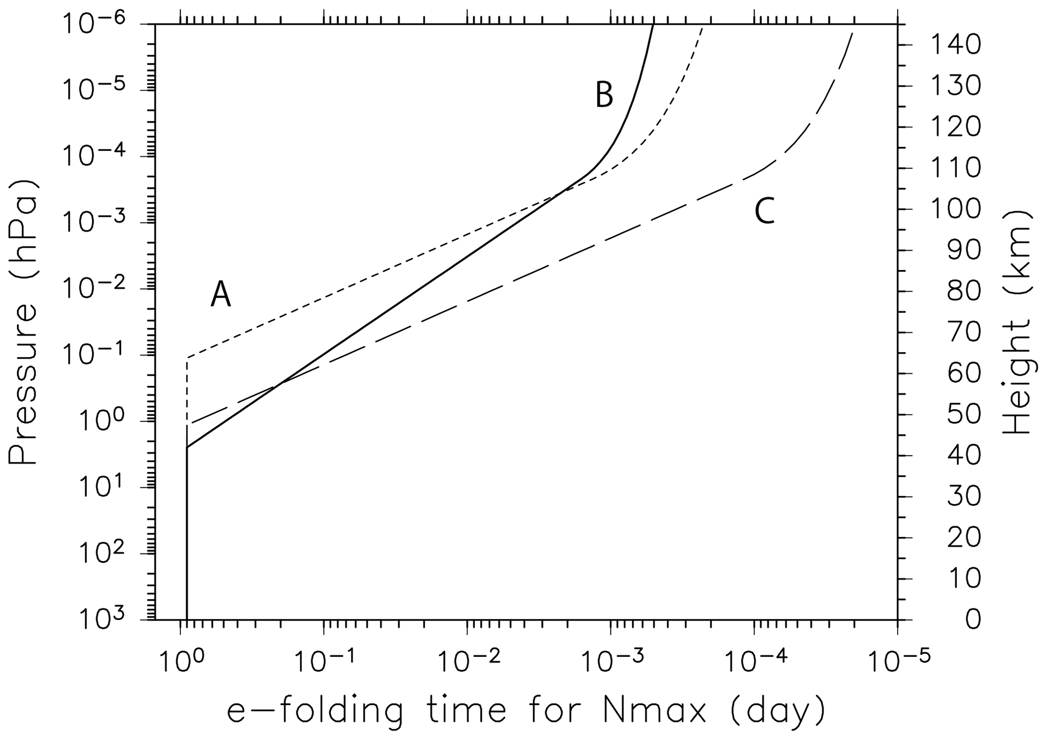
Figure 1 The vertical profiles of the horizontal diffusion coefficients given in the forecast model. Profile B was used for the data assimilation.

Figure 1 shows the three vertical profiles of the horizontal diffusion coefficient. The horizontal axis denotes the e-folding time at the highest resolved wavenumber (total wavenumber n=42). Note that a smaller value on the horizontal axis means stronger horizontal diffusion. The standard diffusion profile of the JAGUAR is denoted by A: the horizontal diffusion coefficient is constant below ∼ 65 km (0.1 hPa) and rapidly increases above. For this setting, we found synoptic-scale disturbances with large amplitudes that are not observed in the free runs around 0.1 hPa. To reduce the amplitudes of the waves, we performed experiments using two other vertical profiles of the horizontal diffusion coefficient denoted by B and C. The diffusion in the B and C profiles is stronger than A below ∼ 60 km, but the increase in the diffusion for B is small compared to A. The diffusion for B is smaller than A above ∼ 105 km. We also performed model runs with other diffusion profiles. We show results of the first (B) and second best (C) profiles as well as the default one.

A free run was performed using the model with each diffusion coefficient profile. The model fields at 00:00 UTC on 5 January of the climatological simulation were used for the same initial condition for the three free-run experiments. The results are examined for the zonal mean model fields averaged over 40 d from 00:00 UTC on 12 January to 23:59 UTC on 20 February at 68.4^∘ S as shown in Fig. 2. Zonal winds observed by the PANSY radar (69.0^∘ S, 39.6^∘ E) and zonal mean zonal winds calculated from the geopotential height of the MLS observation at 67.5–72.5^∘ S assuming the gradient wind balance are also plotted for comparison. We confirmed that similar results are obtained if we take a slightly different latitude and/or a slightly wider latitude range for the model and MLS data. The interannual variation, such as the SSW in the northern-latitude winter, and the intra-annual variation, such as the QBO in the equatorial region, are large. In contrast, it is expected that the interannual and longitudinal variations in the Southern Hemisphere in summer are relatively small because the Carney and Drazin theorem indicates that planetary waves from the troposphere cannot propagate in the westward background wind in the middle atmosphere. This is the reason we compared the observation and model only for the Southern Hemisphere.

Figure 2 Vertical profiles of the zonal mean zonal wind averaged for the time period of 12 January to 20 February from free runs with different horizontal diffusions (A: green curves, B: red curves, C: blue curves) for (a) 2016, (b) 2017, and (c) 2018. PANSY radar and MLS observations are also shown by black solid curves and dashed curves, respectively. Gray shading denotes the range of standard deviation for the PANSY radar observation during the time period. (d) Results of the data assimilation with the Ctrl parameter set for 2017.

It is also worth noting that the vertical axis in Fig. 2 denotes the geometric altitude. The log–pressure height vertical coordinate commonly used in GCM studies is approximately 5 km higher than the geometric height in the upper mesosphere at high latitudes. This difference is taken into account using the model's geopotential height as the vertical coordinate for comparison with the radar wind data, which are obtained as a function of geometric height.

The zonal wind for the experiment with the A profile is more eastward above 87 km and more westward below 85 km than observations. As a result, the vertical shear below 87.5 km is unrealistically strong. In contrast, the results of the experiments with the B and C diffusion profiles show similar profiles as the observations. The difference between the B and C experiments is observed in the vertical shear of zonal wind in the displayed upper mesosphere, which is large for B and small for C. The vertical shear is more realistic for B, although the wind magnitude itself is more realistic for C. We take B because this experiment has a zero-wind layer around 87 km, which is absent in the C experiment, as the zero-wind layer is an important feature observed in the upper mesosphere. We expect the model with the B diffusion coefficient profile to produce realistic vertical wind shear and hence potentially produce realistic wind fields including the zero-wind layer using the data assimilation.

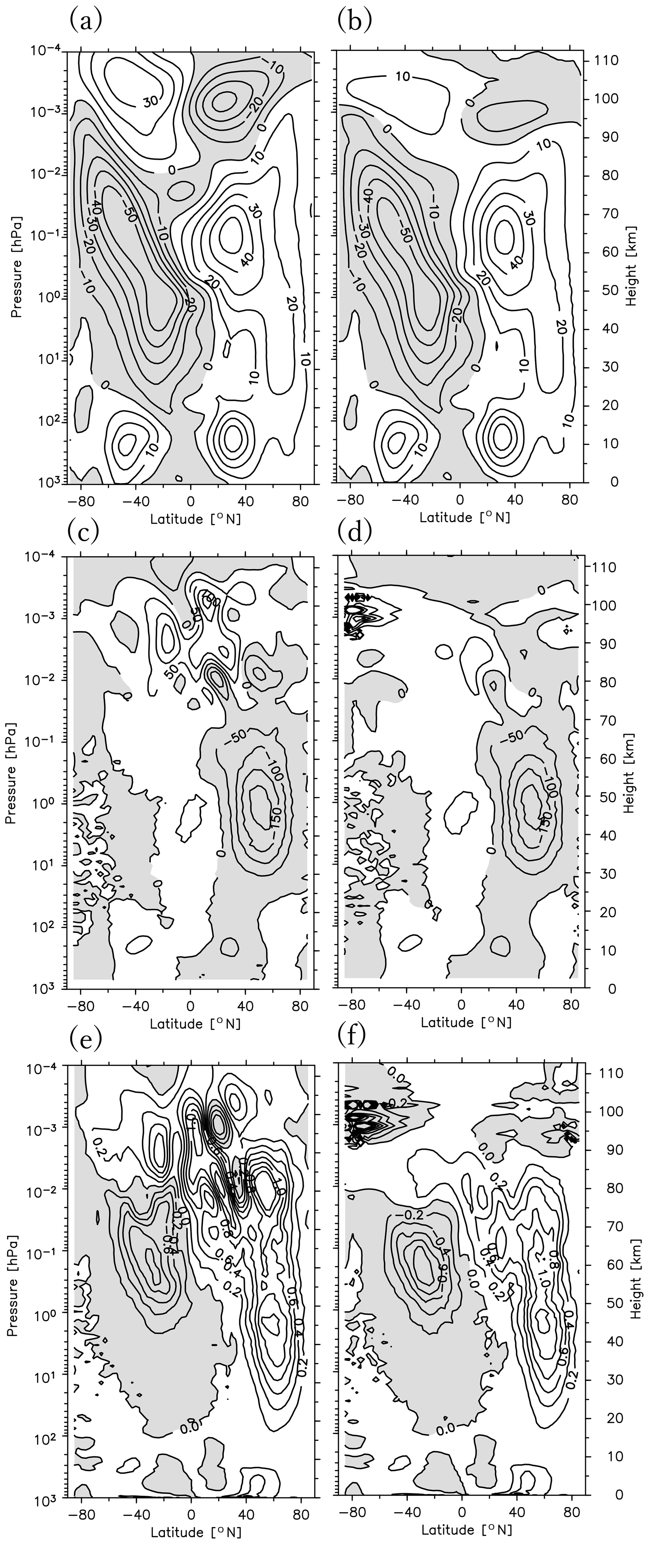
Figure 3 The meridional cross sections of the zonal mean zonal wind (a, b), the meridional component of the E–P flux (c, d), and the vertical component of the E–P flux (e, f). The images in panels (a), (c), and (e) (b, d, and f) were obtained using the results of the data assimilation for DB (Ctrl) (DC) and averaged for the time period of 12 January to 20 February 2017. Contour intervals are 10 m s⁻¹ for (a) and (b), 50 m² s⁻² for (c) and (d), and 0.2 m² s⁻² for (e) and (f).

Figure 2d shows the results of the data assimilation experiments with the B and C diffusion profiles for the time period of 12 January to 20 February 2017. The best set of parameters except for the diffusion profiles in the data assimilation, which will be shown later in detail, was used for these experiments. The results from the B experiment are more realistic in the vertical shear and the location of the zero-wind layer than those of the C experiment, although the difference is not large. Further comparison is performed for the latitude–height cross section of zonal mean zonal wind and Eliassen and Palm (E–P) flux (Fig. 3) from the data assimilation with the B (left) and C (right) diffusion profiles. The meridional structures for the zonal mean zonal wind and the E–P flux in the stratosphere are similar below ∼ 70 km. The difference is observed above. The zonal mean zonal wind and E–P flux are strongly damped above 70 km for C because of strong diffusion given there. This is probably unrealistic. The vertically fine structure is observed for the E–P flux in midlatitude and high-latitude regions from 90 to 100 km, which is probably not real but due instead to numerical instability. From these results, we concluded that the best profile of the horizontal diffusion coefficient is B.

3.1.2 Gravity wave source intensity

The source intensity in the model's non-orographic gravity wave parameterization is tuned as well. The amplitude of upward-propagating gravity waves increases with increasing altitude due to an exponential decrease in the atmospheric density. In the upper mesosphere, breaking gravity waves cause strong forcing to the background winds, which maintains the weak wind layer near the mesopause (Fritts and Alexander, 2003). As the gravity waves, which affect the mesosphere most in the summer, are non-orographically generated, we tuned the source intensity of the non-orographic gravity wave parameterization. It is expected that high source intensity lowers the wave breaking level and hence lowers the weak wind layer around the mesopause.

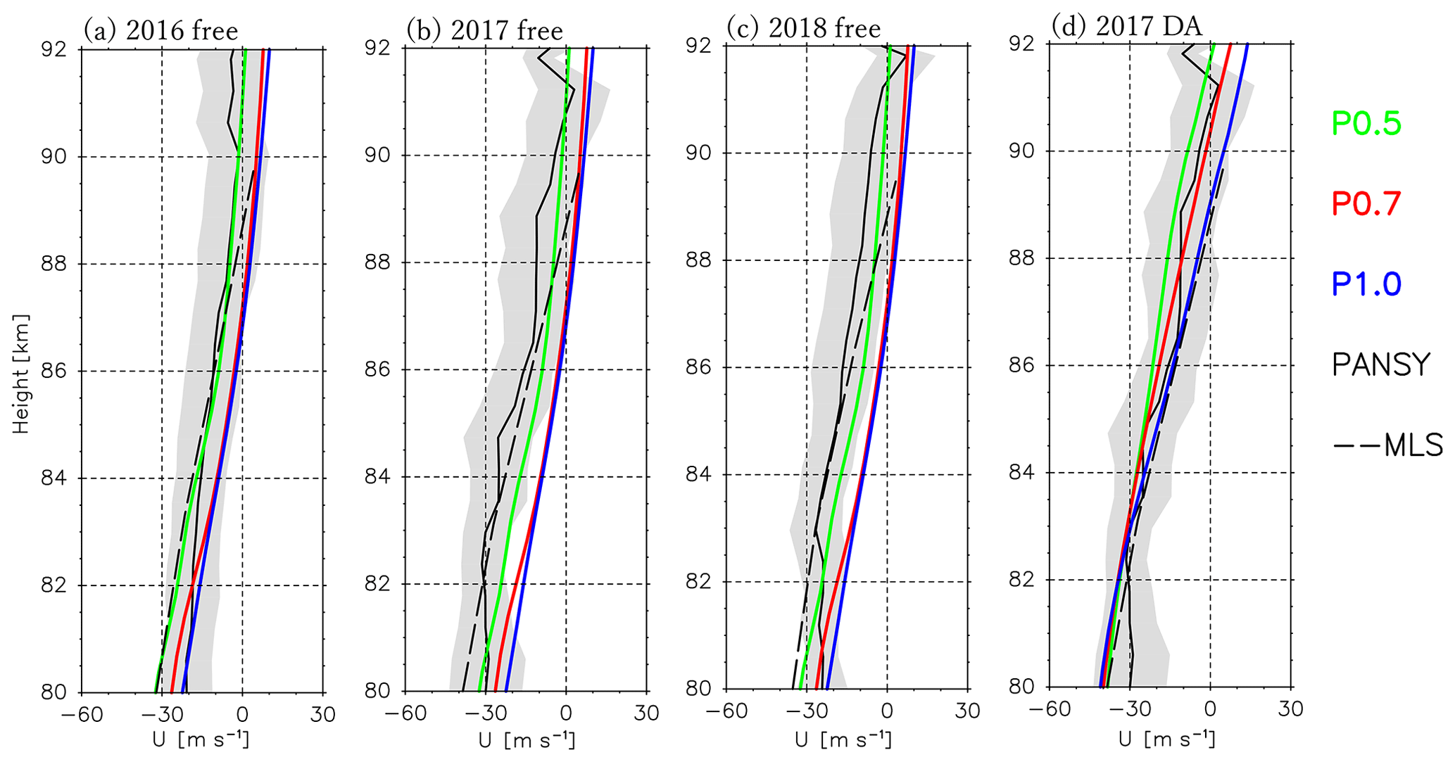
Figure 4 The vertical profiles of the zonal mean zonal wind averaged for the time period of 12 January to 20 February from free runs with gravity wave parameterizations of different source intensities (P0.5: green curves, P0.7: red curves, P1.0: blue curves) for (a) 2016, (b) 2017, and (c) 2018. PANSY radar and MLS observations are also shown by black solid curves and dashed curves, respectively. Gray shading denotes the range of standard deviation for the PANSY radar observation during the time period. (d) Results of the data assimilation with the Ctrl parameter set for 2017.

Figure 5 The day–latitude section of MLS bias at (a) 10 hPa, (b) 1 hPa, (c) 0.1 hPa, and (d) 0.01 hPa. The contour intervals are 0.5 K.

Figure 4a compares vertical profiles of the zonal mean zonal wind at 68.37^∘ S averaged for the time period of 12 January to 20 February from free runs with different source intensities of the non-orographic gravity wave parameterization. The original source intensity is denoted by P1.0, and the modified intensities are 0.5 and 0.7 times the original source intensity, denoted by P0.5 and P0.7, respectively. The PANSY radar and MLS observations are plotted for comparison similar to Fig. 2. Results of the climatological simulation are used as the initial condition for the free run, which is the same as for the free-run experiments with different horizontal diffusion coefficients.

As we expected, the zonal mean zonal wind is weaker and the height of the zero-wind layer is lower for stronger source intensity. It seems that the zonal wind is weaker and the zero-wind layer is lower for P1.0 than those in the observations.

Figure 4d shows the results of the data assimilation experiments with P0.5, P0.7, and P1.0 for the time period of 12 January to 20 February 2017. For these experiments, the best set of parameters except for the source intensity was used in the data assimilation, which will be shown later in detail. Although all the profiles are consistent with observations within the standard deviation range, the profile for P0.7 is the most similar to observations in terms of the magnitude and the height of the zero-wind layer. From these results, we determined that the best source intensity is 0.7 times the original one (i.e., P0.7).

3.2 Aura MLS bias correction

According to the Aura MLS data quality document (Livesey et al., 2018), the MLS temperature data have a bias compared to the SABER ones as a function of the pressure, which is −5 to +1 K for pressure levels of 1–0.1 hPa, −3 to 0 K for 0.1–0.01 hPa, and −10 K for 0.001 hPa. Thus, before performing the data assimilation, the MLS observation bias was removed as much as possible. Previous studies treated the bias correction in various ways: Hoppel et al. (2008) used bias-corrected SABER (v.1.06) data with the MLS data (v.2.2). Eckermann et al. (2009) used SABER (v.1.07) and MLS (v.2.2) temperatures for their assimilation in which the SABER (v.1.07) temperatures at altitudes below 2.7 hPa were bias-corrected using the mean difference from MLS (v.2.2), and the MLS temperatures above 2 hPa were bias-corrected using the mean difference relative to other satellite, suborbital, and analysis temperatures. Note that these studies used different versions of the SABER data (v.1.0X) from that we used (v.2.0). Pedatella et al. (2014b) did not perform the bias correction. Pedatella et al. (2016) adjusted the SABER temperatures to account for the bias between SABER (v.2.0) and MLS (v.2.2) temperatures. Eckermann et al. (2018) performed a bias correction for the MLS temperatures (v.4.0) above 5 hPa using the mean difference between MLS and SABER (v.2.0) temperatures, as well as the SABER temperatures for the pressure levels from 68 to 5 hPa using the mean difference between MLS and SABER. McCormack et al. (2017) and Pedatella et al. (2018) do not state explicitly whether or not a bias correction is applied, so it is not clear which bias correction was performed in their studies. We confirmed that the bias estimated in this study is similar to the globally averaged mean differences between MLS temperature and other correlative datasets shown in the data quality document (Liversey et al., 2018) at each height.

In this study, the MLS observation bias is first estimated as a function of the calendar day at each latitude and each pressure in a range of 177.838 to 0.001 hPa. As the reference for the correction, we used the TIMED SABER temperature data (v.2.0), which are considered to have little observation bias, at least in the altitude range from 85 to 100 km, as confirmed by Xu et al. (2006), who used data from the sodium lidar at Colorado State University, providing the absolute value of the temperature. Xu et al. (2006) attributed the disagreement below 85 km to high photon noise contaminating the lidar observations. Thus, we used the SABER temperature data for the Aura MLS bias estimation in the height range of 10–100 km.

The observation view of SABER is altered every ∼ 60 d by switching between northward (50^∘ S–82^∘ N) and southward (82^∘ S–50^∘ N) view modes. Thus, the latitudinal coverage of the SABER data is narrow compared to the MLS data. However, both datasets overlap for a long time period sufficient for statistical comparison between them.

The bias is estimated using data from 2005 to 2015. The original vertical resolution of MLS (∼ 1–5 km) is coarser than that of SABER (∼ 0.5 km). First, the vertical mean of the SABER data corresponding to the vertical resolution at each of the 55 height levels of MLS data is obtained. Next, by linear interpolation, data at the grid of 25^∘ (longitude) × 5^∘ (latitude) at a time interval of 3 h are made for MLS and SABER data. The MLS and SABER data made at a 3 h interval have a lot of missing values because observations are sparse. These missing values are not used for the bias calculation. This means that the bias was estimated using MLS and SABER data at nearly the same local time. Whereas the longitudinal variation of the bias is small (1 K at the most), there is large annual variation in addition to the dependence on latitude and height. Thus, the MLS bias T_bias is obtained as a function of the latitude (y), height (z), and calendar day (t):

$$\begin{array}{rl}{T}_{\mathrm{bias}}\left(y,z,t\right)& =T_{\mathrm{mean}}\left(y,z\right)+A\left(y,z\right)\cos \left(\mathrm{2}\mathit{\pi }{\displaystyle \frac{t}{\mathrm{365}}}\right)\\ & +B\left(y,z\right)\sin \left(\mathrm{2}\mathit{\pi }{\displaystyle \frac{t}{\mathrm{365}}}\right),\end{array}$$

where T_mean represents the annual mean, and the coefficients A and B are estimated by the least-squares method.

Figure 6 The vertical profile of the global average of the Aura MLS temperature bias (the solid black curve) with standard deviation (gray shading). Error bars denote reported bias (Livesey et al., 2018).

Figure 5 shows the estimated MLS bias as a function of calendar day and latitude at 10, 1, 0.1, and 0.01 hPa. The MLS bias shows a strong dependence on the altitude and latitude and has an annual cycle with amplitudes of 2 to 4 K. Figure 6 shows the vertical profiles of global mean Aura MLS bias along with the bias reported in the data quality document (Liversey et al., 2018). For example, the global mean MLS biases estimated by the present study are $-\mathrm{1.6}\pm \mathrm{0.7}$ K at 56.2 hPa, 2.0±1.4 K at 1 hPa, and $-\mathrm{3.8}\pm \mathrm{1.1}$ K at 0.316 hPa. These are comparable to the biases described in the data quality document, which are −2 to 0 K at 56.2 hPa, 0 to 5 K at 1 hPa, and −7 to 4 K at 0.316. This consistency indicates the validity of using the SABER data as a reference to estimate the MLS bias.

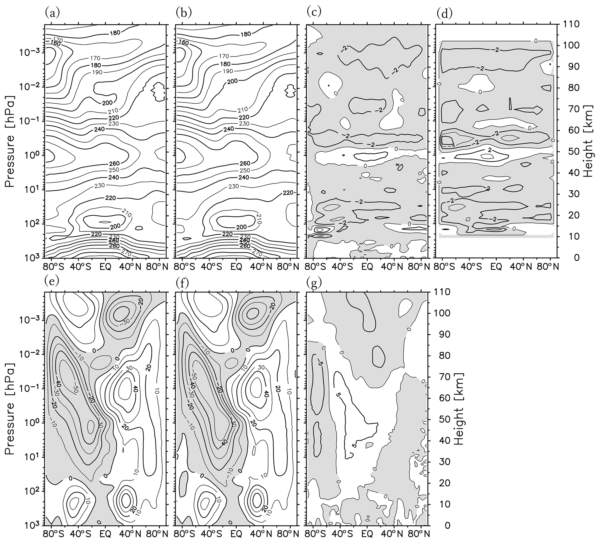
Figure 7 The meridional cross sections of zonal mean temperature (a, b) and zonal wind (e, f). The results in panels (a) and (e) (b and f) are from assimilating Aura MLS data without (with) bias correction, which are averaged for the time period of 12 January to 20 February 2017. (c) The difference between (a) and (b); (g) difference between (e) and (f). (d) The corrected bias for the same time period. Contour intervals are 10 K for (a) and (b), 2 K for (c) and (d), 10 m s⁻¹ for (e) and (f), and 5 m s⁻¹ for (g).

To evaluate the effect of the bias correction, data assimilation was performed using the MLS data with and without bias correction. Figure 7 compares the latitude and pressure section of the zonal mean temperature and zonal wind between the two analyses. The difference in zonal mean temperature between the two (Fig. 7c) resembles the corrected bias (Fig. 7d). In contrast, the difference in the zonal mean zonal wind is not very large (Fig. 7g). This is because the latitudinal difference in the bias, which largely affects the zonal mean zonal wind through the thermal wind balance, is not large compared to the vertical difference. In our study, the bias correction of the MLS data is made before the data assimilation, as in standard assimilation parameter setting.

3.3 Data assimilation setting optimization for 30 ensemble members

A series of sensitivity tests were performed to obtain the best values of each parameter in the data assimilation system with 30 ensemble members. This number of members is practical for the data assimilation up to the lower thermosphere with current supercomputer technology. The examined assimilation parameters are the gross error coefficient, localization length, inflation coefficient, and assimilation window length. The best parameter set obtained by the sensitivity tests is denoted by Ctrl in Table 1. There are six assimilation parameters to be examined. We performed an assimilation run with almost all combinations of the parameters. Several parameter settings did not work due to computational instability. We found a parameter set that provides the best assimilation results in our system. This best parameter set is placed as the control setting (Ctrl), and the parameter dependence of the assimilation performance is examined by using the results in which one of the parameters is changed from the Ctrl set. Section 3.3.5 gives a short summary of the data assimilation setting optimization for 30 ensemble members.

3.3.1 Gross error coefficient

The gross error check is a method of quality control (QC) for the observation data used for the assimilation. In this method, an observation is assimilated only if its OmF is smaller than expected, assuming that the forecast model provides a reasonable representation of the true atmosphere. In many previous studies, observations are not assimilated when the OmF exceeds 3–5 times the observational error for the troposphere and stratosphere. However, this criterion may not be suitable for the mesosphere and lower thermosphere, in which the systematic bias and predictability of the model are likely higher and lower, respectively (e.g., Pedatella et al., 2014a). Thus, the maximal allowable difference between the MLS observations and model forecasts normalized by the observational error, which is called the “gross error coefficient”, is set at 20 (hereafter referred to as the G20) for the MLS measurements as a control experiment of the present study, whereas it is set at 5 for the PREPBUFR dataset as in previous studies such as Miyoshi et al. (2007). Consequently, this setting uses most of the MLS observations to correct the model forecast. To investigate the effect of the enlarged gross error check coefficient, the result for the G20 is also compared to the experiment with the gross error coefficient of 5 for the MLS measurement (G5). Note that the other parameters in addition to the gross error coefficient are taken to be the same for the G20 (Ctrl) and G5 (see Table 1).

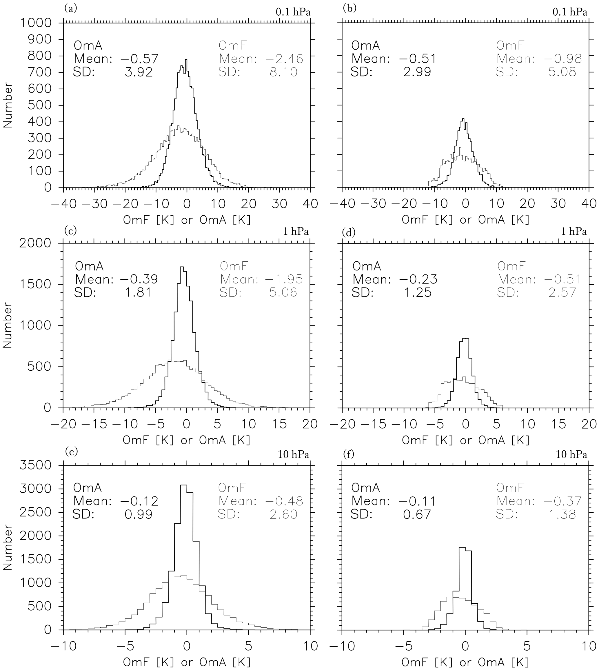
Figure 8 Histogram of the OmF (thin curves) and OmA (thick curves) at 0.1 hPa (a, b), 1 hPa (c, d), and 10 hPa (e, f). Panels (a), (c), and (e) are the results from G20 (b, d, and f for G5) for the time period of 12 January to 20 February 2017.

Figure 8 compares the histograms of the OmF (a gray curve) and OmA (a black curve) for the G20 (left) and G5 (right) experiments at 0.1, 1, and 10 hPa. For both settings, the mean OmF values are slightly negative, whereas both the mean bias and standard deviations of the OmA are smaller than those of the OmF at most pressure levels. As expected, the OmF is more widely distributed for the G20 than for the G5. This reflects the inclusion of more observations for the assimilation with the G20. Although the OmF distribution for the G20 is close to the normal distribution, the distribution of for the G5 seems distorted, probably by an overly strict selection of observations close to the model forecasts, which can be seen from the number of assimilated observations, as indicated by the area of the histogram in Fig. 8, which is only a half or a third the number for the G20.

Figure 9 shows vertical profiles of the mean OmF, OmA, and χ² (see Sect. 2.4). Absolute values of the mean OmA are smaller than those of the mean OmF at almost all levels for both the G20 and G5 experiments. Note that the bias of the OmA is smaller than the standard deviation, as shown in Fig. 8 as an example. The absolute values of the mean OmF for the G20 are 1.5–2 times larger than those for the G5, implying that more observations that deviate largely from the forecasts are assimilated for the G20. It is worth noting that the absolute value of the mean OmF tends to increase with height, indicating that the forecast is less reliable in the upper stratosphere and mesosphere. The χ² values with the G20 are larger than those with the G5 at all levels, reflecting a larger OmF for the G20. Generally speaking, such large χ² values with the G20 suggest that optimizing observation error and forecast spread is required. However, considering the current immature stage of the forecast model performance in the upper mesosphere and above, we permitted the large χ² values with the G20, as it allows us to use a large number of observations, which are sparse in the upper stratosphere and mesosphere. In fact, the correlation between our analysis and observation is greatly improved for the G20 compared with the G5 (shown later in Fig. 15). It will be shown later that the χ² values are improved by taking a larger number of ensemble members.

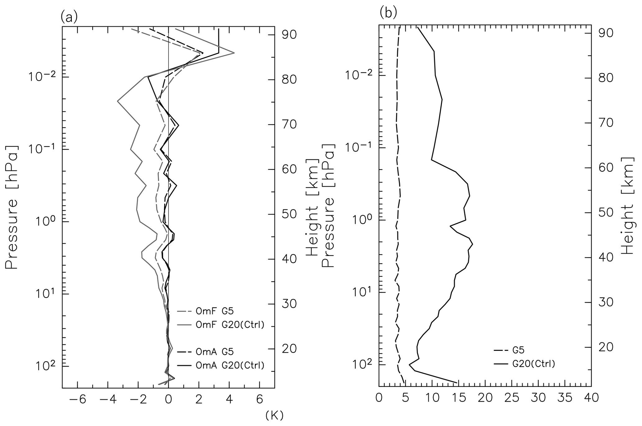
Figure 9 The vertical profiles of the global mean (a) OmF and OmA, as well as (b) χ². The gray (black) curves denote the OmF (OmA) in (a). Dashed and solid curves denote results from the G5 and G20 (Ctrl), respectively. Plotted is an average for the time period of 12 January to 20 February 2017.

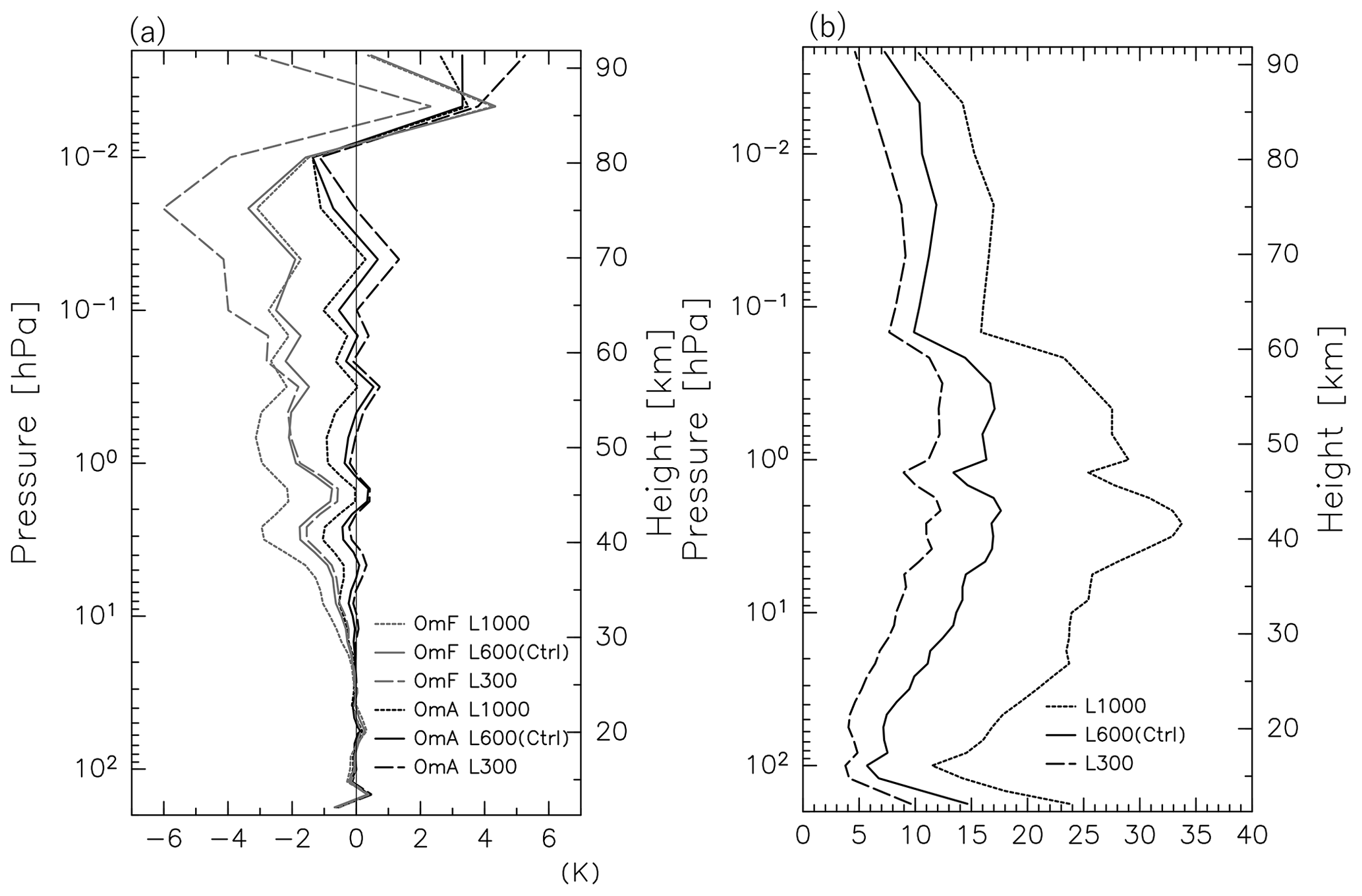
Figure 10 The vertical profiles of the global mean (a) OmF and OmA, as well as (b) χ². The gray (black) curves denote the OmF (OmA) in (a). Dashed, solid, and dotted curves denote results from L300, L600 (Ctrl), and L1000, respectively. Plotted is an average for the time period of 12 January to 20 February 2017.

3.3.2 Localization length

In the LETKF, the observation error is weighted with the inverse shape of the Gaussian function (observational localization) of the distance (d) between the location of the observation and the grid point:

$$\begin{array}{}\text{(23)}& R^{\prime }=R\cdot \exp \left[{\displaystyle \frac{d^{\mathrm{2}}}{\mathrm{2}{L}^{\mathrm{2}}}}\right],\end{array}$$

where R and R^′ are the original and modified observation error covariances, respectively, and L is a horizontal length scale that describes the distance to which the observation is effective in the assimilation. The parameter L is called the “localization length”, which is one of the key parameters that determine the LETKF performance. For a forecast model with a high degree of freedom, as in the present study, a small number of ensemble members may cause sampling errors in the forecast error covariance at a long distance (e.g., Miyoshi et al., 2014). The localization is introduced to reduce such spurious correlations at long distances.

A sensitivity test is performed by taking L=300 km (L300), L=600 km (L600, Ctrl), and L=1000 km (L1000) without changing the other parameters (see Table 1). For the vertical localization length, we used the same setting for all experiments. It is defined by the inverse of the Gaussian function (Eq. 23), with L=0.6 and $d=\ln (p_{\mathrm{obs}}/p_{\mathrm{0}})-\ln (p_{\mathrm{grid}}/p_{\mathrm{0}})$, where p_obs, p_grid, and p₀ are the pressures of the observation, grid point, and surface, respectively. Figure 10 shows the vertical profiles of the mean OmF, OmA, and χ² for the L300, L600 (Ctrl), and L1000. The magnitude of the mean OmF is largest for the L1000 below 0.3 hPa and for the L300 above between the three experiments. The OmA values are distributed around zero for L600, whereas they tend to be negative for the L1000, particularly at lower levels, and tend to be positive for the L300, particularly at upper levels. The χ² values are smallest for the L300 and largest for the L1000.

Table 2 The localization length dependence of the root mean square (RMS) difference (K) between the analysis temperature and the MLS temperature observation. The averaged data for the time period of 12 January to 20 February 2017 are shown.

This result suggests that the best localization length depends on the height. To see the height dependence in a different way, the root mean square (RMS) of the temperature difference from the (bias-corrected) MLS observations was calculated for each experiment at each height. Results are shown in Table 2 for typical levels of 10, 1, 0.1, 0.01, and 0.005 hPa in the stratosphere and mesosphere. A smaller RMS means that observations are better assimilated. The RMS is smallest for the L300 at lower levels of 10 and 1 hPa, for the L600 at 0.1 hPa, and for the L1000 at upper levels of 0.01 and 0.005 hPa, suggesting that optimal localization length depends on the height.

Based on the results, we employed the L600 as the best L to obtain a better analysis for all levels from the stratosphere to the upper mesosphere. Our assimilation does not necessarily provide the best analysis data for a limited height region, but it does ensure that the analysis has a sufficient, nearly uniform quality for the whole middle atmosphere.

3.3.3 Inflation coefficient

To avoid possible underestimations in the forecast error covariances due to the small number of ensembles used in the assimilation, a covariance inflation technique is employed (see Eq. 9). The inflation coefficient is generally set to ∼ 10 % for the tropospheric system (e.g., Miyoshi et al., 2007; Miyoshi and Yamane, 2007; Hunt et al., 2007). We tested three different inflation coefficients, namely 7 % (I7), 15 % (I15, Ctrl), and 25 % (I25). Note again that the sensitivity test was conducted by changing the inflation coefficient only (see Table 1).

Figure 11 shows meridional cross sections of the zonal mean ensemble spread of temperature for each assimilation run. The ensemble spread for the I7 is about 1 K at most in the mesosphere and lower thermosphere, which is smaller than the observation accuracy (1–3 K). In contrast, the ensemble spreads for the I15 and I25 are distributed in the range of the observation accuracy. The necessity of a larger inflation coefficient is likely due to the large diffusion coefficient in the upper mesosphere and lower thermosphere used in the forecast model (Fig. 1). However, a larger inflation coefficient leads to an unrealistically thin vertical structure of ensemble spreads in the lower mesosphere, which is conspicuous for the I25 (Fig. 11). Figure 12 shows the time series of the global mean temperature spreads for respective settings at 0.01 and 10 hPa. The temperature spreads vary slightly in time and seem stable after 13 January for both pressure levels.

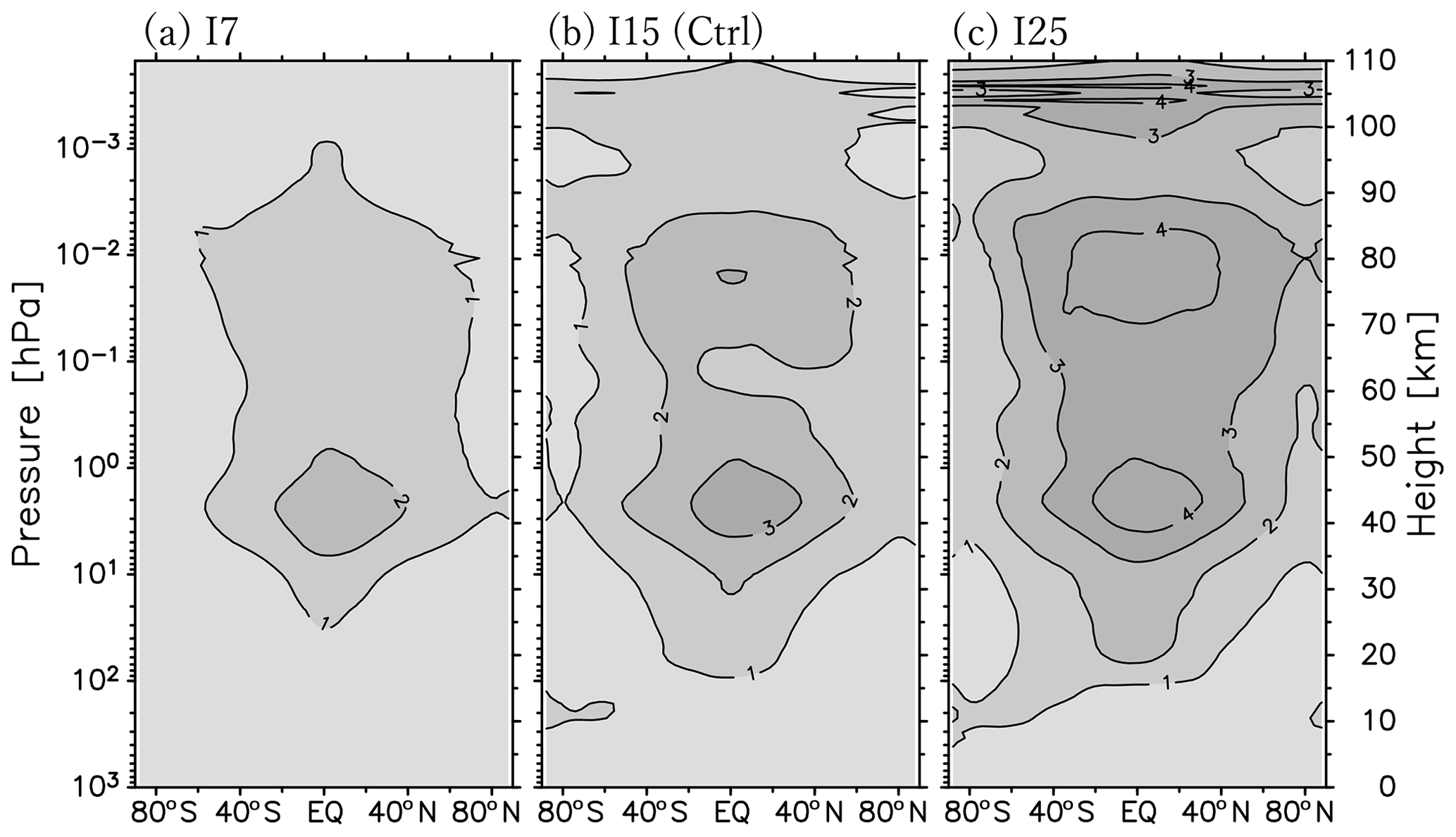
Figure 11 The meridional cross section of the zonal mean ensemble spread of temperature (K) for (a) I7, (b) I15 (Ctrl), and (c) I25 averaged for the time period of 12 January to 20 February 2017.

Figure 12 The time series of the global mean temperature spread for (a) 0.01 hPa and (b) 10 hPa. Dashed, solid, and dotted curves denote results from I7, I15 (Ctrl), and I25, respectively.

The vertical profiles of the mean OmF, OmA, and χ² for the I7, I15, and I25 are shown in Fig. 13. The absolute value of the OmF and OmA is the smallest for the I15 at most altitudes. The χ² values are also small for the I15 at most altitudes. Thus, we employed the best inflation coefficient of 15 % (i.e., I15).

Interestingly, the range of the best inflation coefficient also depends on the height from a viewpoint of χ²: the χ² values for the I15 are similar to those for the I25 but smaller than the I5 above 0.2 hPa, whereas they are similar to those for the I7 but smaller than the I25 below 0.2 hPa.

3.3.4 Assimilation window length

The length of the assimilation window, which is a time duration of forecast and observation to be assimilated during one assimilation cycle, is also examined. When the assimilation window is set to 6 h, the forecast is first performed for t=0–9 h, and next the analysis at t=6 h is obtained by the assimilation using the forecasts and observations for the time period of t=3–9 h in the assimilation. Note that this assimilation scheme uses future information to obtain the analysis at a certain time. The obtained analysis is used as an initial condition for the next forecast for 9 h (i.e., t=6–15 h). By repeating these processes of forecast and assimilation, an analysis is obtained every 6 h. Thus, the length of the assimilation window determines the length of the forecast run as well as the analysis interval.

A longer window has the advantage that more observations are assimilated at once, while taking the predicted physically balanced time evolution of dynamical fields into account. However, the longer forecast length may increase model errors. Moreover, the 4D-EnKF assumes a linear time evolution of the dynamical field during the assimilation window length. Thus, variations with strong nonlinearity or with timescales shorter than the assimilation window length are not taken into account. We tested assimilation windows of 3 h (W3), 6 h (W6, Ctrl), and 12 h (W12) (see Table 1). The W12 (W3) assimilation was performed using the forecasts for t=6–18 h (t=2–4 h) out of the forecast run over 18 h (4 h) and the corresponding observations.

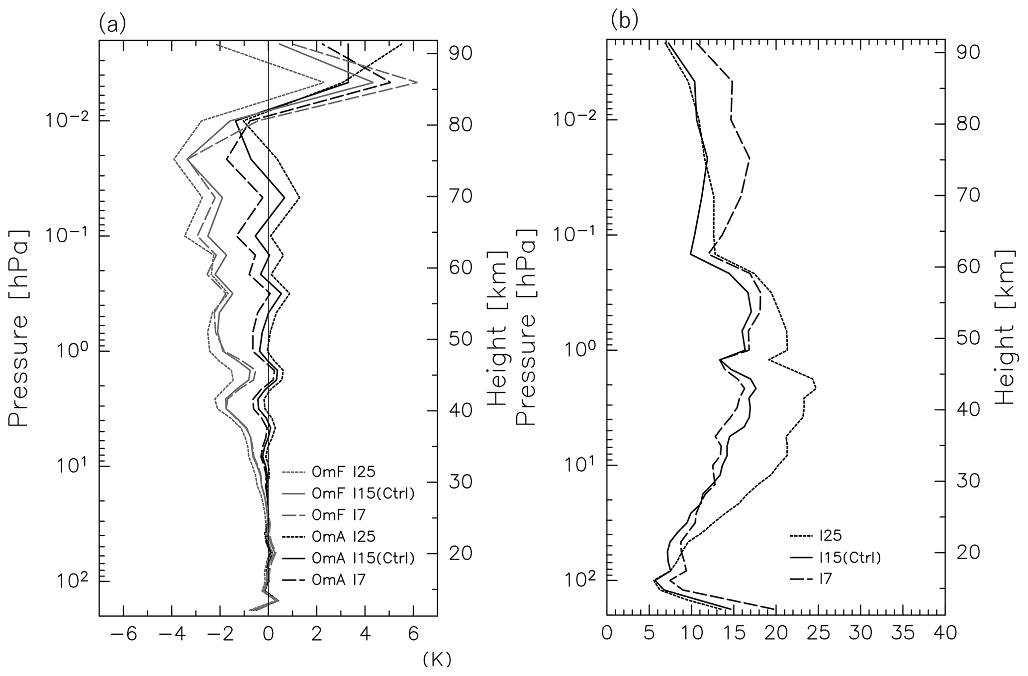
Figure 13 The vertical profiles of the global mean (a) OmF and OmA, as well as (b) χ². The gray (black) curves denote the OmF (OmA) in (a). Dashed, solid, and dotted curves denote results from I7, I15 (Ctrl), and I25, respectively. Plotted is an average for the time period of 12 January to 20 February 2017.

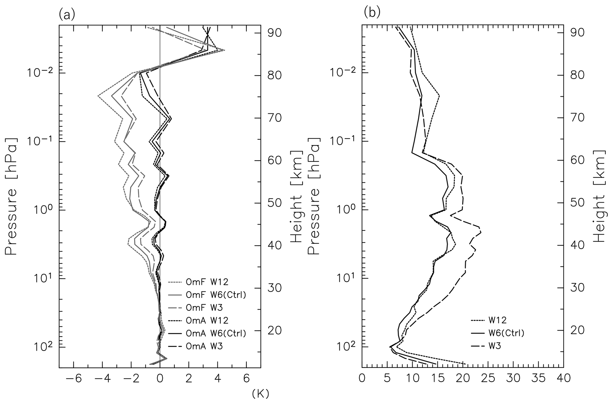
Figure 14 The vertical profiles of the global mean (a) OmF and OmA, as well as (b) χ². The gray (black) curves denote the OmF (OmA) in (a). Dashed, solid, and dotted curves denote results from W3, W6 (Ctrl), and W12, respectively. Plotted is an average for the time period of 12 January to 20 February 2017.

Figure 14 shows the vertical profiles of the mean OmF, OmA, and χ² for the three assimilations. The OmF for the W3 (W12) is calculated using the forecast for 3 h (12 h), while for the other experiments, whose assimilation window is 6 h, the forecast for 6 h is used. The mean OmF and OmA values for the W6 and W12 are larger than for the W3, suggesting larger forecast errors in longer windows. There are two possible reasons: first, forecast error is generally larger for a longer forecast time at a certain parameter setting. Second, relatively short-period disturbances such as quasi-2 d waves are dominant, particularly in the mesosphere (e.g., Pancheva et al., 2016), which requires a short assimilation window for their expression. However, χ² is significantly larger for the W3 than for the W6 and W12, particularly below 0.2 hPa, suggesting that the 3 h window may have been too short to develop forecast error spreads sufficiently, especially for the lower atmosphere. Based on these results, the length of 6 h is regarded as the best assimilation window.

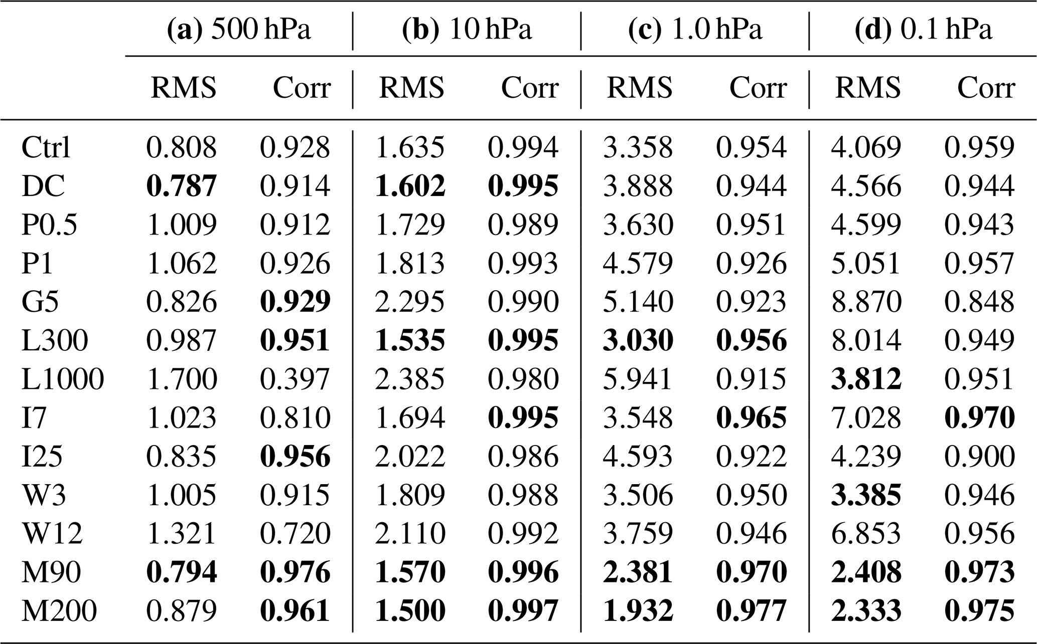
Table 3 The bias of the time series of zonal mean temperature at 70^∘ N for the time period from 15 January to 20 February 2017 from each assimilation experiment and from MERRA-2 (see Fig. 15). The RMS of the differences between the time series of each experiment and MERRA-2, as well as the correlation (Corr) between the time series from each experiment and from MERRA-2, is also shown. Results for (a) 500 hPa, (b) 10 hPa, (c) 1 hPa, and (d) 0.1 hPa are shown. The numerals showing a better performance than Ctrl are boldfaced.

3.3.5 Comparison of a series of sensitivity tests for data assimilation with 30 ensemble members

In Sect. 3.3.1 to 3.3.4, a series of sensitivity tests for each parameter in the data assimilation system with 30 ensemble members was performed as shown in Table 1. Figure 15 shows the time series of the zonal mean temperatures at 70^∘ N for 500, 10, 1, and 0.1 hPa for the time period of 15 January to 20 February 2017 from the respective assimilation tests shown in Table 1 (black curves). Gray curves represent the time series from MERRA-2. Using the time series shown in Fig. 16, the RMSs of the differences and correlations between the time series of each run and MERRA-2 are calculated and summarized in Table 3. The criteria of the major SSW were satisfied on 1 February.

The Ctrl time series is also quite similar to that of MERRA-2 in spite of the small number of ensemble members, including drastic temperature change during the major SSW event, although a warm bias of ∼4 K is observed at 0.1 hPa before and after the cooling time period associated with the warming at 10 hPa. It is worth noting that the G5 has a significant warm bias: ∼4 K at 10 hPa from 31 January to 5 February during the warming event, ∼10 K at 1 hPa on 23 January when a sudden temperature drop was observed, and ∼10 K at 0.1 hPa before and after the cooling time period (i.e., before 27 January and after 6 February). Such significantly large biases are probably due to the model bias because they are not observed for the Ctrl run, in which a much larger number of observations was assimilated.

3.4 The effect of ensemble size and an estimate of the optimal ensemble size for the data assimilation in the middle atmosphere

The EnKF statistically estimates the forecast error covariance using ensembles. A large ensemble size (i.e., a large number of ensemble members) is favorable because it reduces the sampling error of the covariance and improves the quality of the analysis. However, the ensemble size has a practical limit related to the allowable computational resources. An ensemble size of ∼ 30 is usually used in operational weather forecasting. Here, the minimum optimal ensemble size is estimated by performing additional experiments with 90 (M90) and 200 (M200) members and comparing them with the Ctrl experiment of 30 members (M30, Ctrl). No assimilation parameters, except for the ensemble size, are changed in the M90 and M200 experiments (see Table 1). Note that the best values of the assimilation parameters for the larger ensemble sizes may be different from those for Ctrl. For example, a larger ensemble size may allow for a larger localization length. However, further investigation was not made because a high computational cost is required.

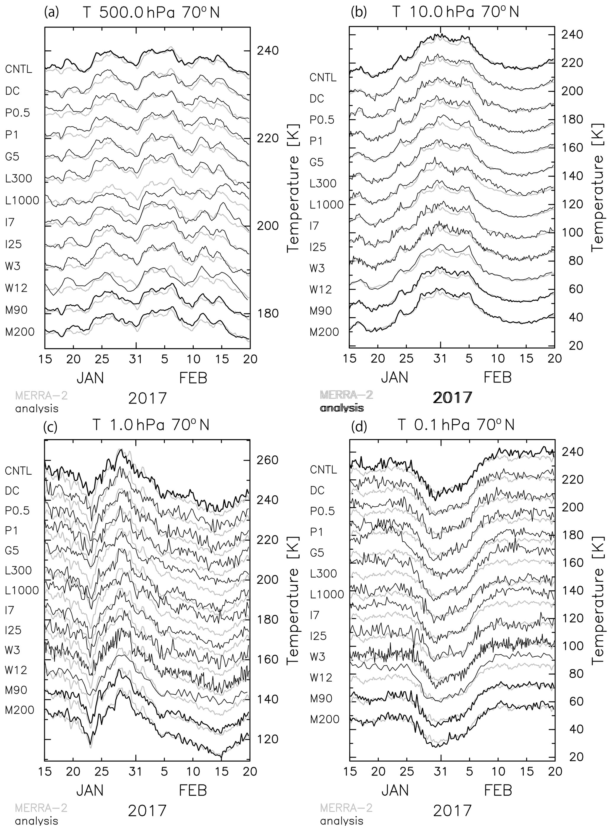
Figure 15 The time series of the zonal mean temperature at 70^∘ N for (a) 500 hPa, (b) 10 hPa, (c) 1 hPa, and (d) 0.1 hPa. The black curves show the results from each parameter setting (see Table 1). The right axis is given for the result of Ctrl, and the other curves are vertically shifted by (a) 5 K, (b) 15 K, (c) 10 K, and (d) 15 K. The gray curves show the time series calculated using MERRA-2 as a reference.

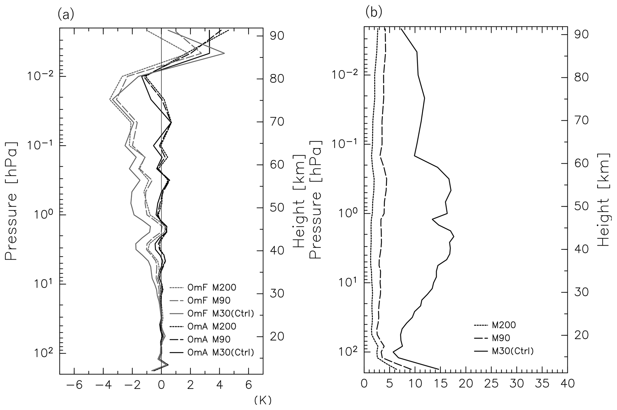
Figure 16 The vertical profiles of the global mean (a) OmF and OmA, as well as (b) χ². The gray (black) curves denote the OmF (OmA) in (a). Dashed, solid, and dotted curves denote results from M30 (Ctrl), M90, and M200, respectively. Plotted is an average for the time period of 12 January to 20 February 2017.

Figure 16 shows the vertical profiles of the mean OmF, OmA, and χ² for the M30 (Ctrl), M90, and M200. The OmFs for the M90 and M200 are significantly smaller than for the M30, particularly below 0.1 hPa (by ∼ 50 %), while the OmAs are comparable for the three runs. The difference between the OmFs of the M90 and M200 runs is small. Although the χ² values are ∼ 6–17 for M30, they are ∼ 3–4 for M90 and ∼ 1–2 for M200, which are close to the optimal values of χ². The reduced values of χ² by increasing the ensemble size are remarkable compared with those by optimizing the other parameters (Sect. 3.3). However, the M90 and M200 both require such large computational costs, as already stated, that they are not available for long-term reanalysis calculations. The time series obtained from the M90 and M200 are also shown in Fig. 15. Both time series agree well with the MERRA-2 time series and do not have even a slight warm bias like that observed at 0.1 hPa in the Ctrl time series.

In the following, an attempt is made to estimate the minimum number of ensemble members as a function of height using forecasts of ensemble members from the M200 experiment because 90 is a sufficient number for high-quality assimilation, judged from the similarity of the performances of the M90 and M200 runs. Figure 17 shows the correlation coefficient of forecasts at each longitude for a reference point of 180^∘ E for 40^∘ N at 10 and 0.01 hPa that are computed using 12, 25, 50, and 100 members randomly chosen from the M200 forecasts at 06:00 UTC, 21 January 2017. The longitudinal profile of the correlation coefficient for 200 members is also shown. The correlation is generally reduced as the distance from the reference point increases, with large ripples for the results of ensemble sizes smaller than 50, although the correlation profile near the reference point is expressed for all the members. Large ripples reaching ±0.6 observed for 12 members are considered spurious correlations caused by the under-sampling. In contrast, the correlation coefficients for 100 and 200 ensemble members are generally smaller than 0.2 except for a meaningfully high correlation region around the reference point. We performed the same analysis for other latitudes and heights and obtained similar results (not shown).

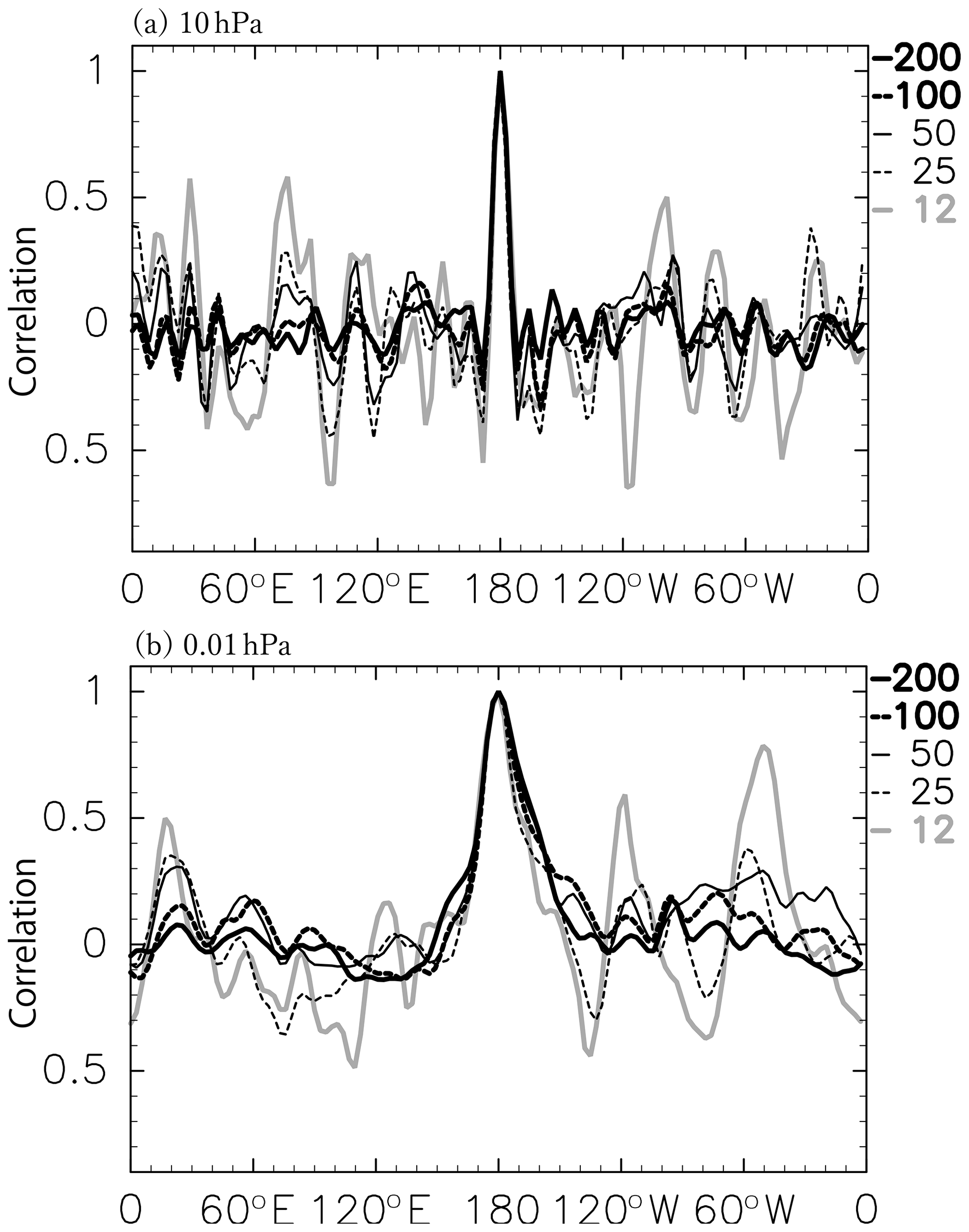
Figure 17 An example of ensemble correlation of temperature. Results for 40^∘ N at 10 hPa (a) and 0.01 hPa (b). Each curve shows the results of the 200 (a thick solid curve), 100 (thick dashed), 50 (thin solid), 25 (thin dashed), and 12 (thick gray) ensembles. We performed the same analysis for other latitudes and heights and obtained similar results.

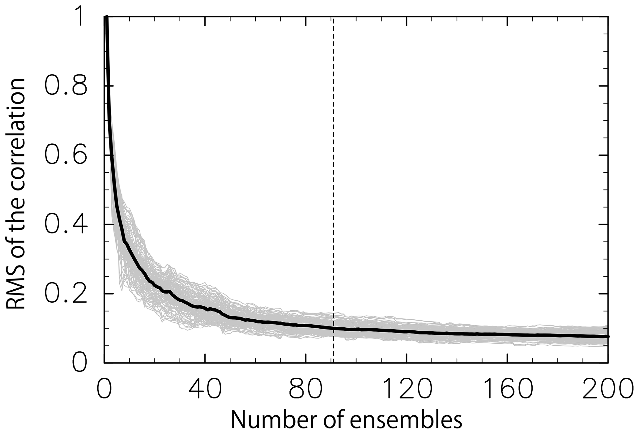
Figure 18 An example of the RMS of spurious correlation. Results for 40^∘ N at 0.01 hPa (06:00 UTC on 21 January 2017) as a function of the number of ensembles. The gray curves show the results of respective longitude, and a black curve shows the average. A dashed line shows the number of members for which the mean RMS is 0.1 (i.e., 91).

The RMS of the spurious correlation in the region outside the meaningful correlation region is used to estimate the minimum optimal number of ensemble members. The RMS is examined as a function of the number of ensemble members. Each edge longitude of the meaningful correlation region is determined where the correlation falls below 0.1 nearest the reference point, which are 171.6^∘ E and 171.6^∘ W for 10 hPa and 149.1^∘ E and 146.2^∘ W for 0.01 hPa for the case shown in Fig. 17. Note that the threshold value 0.1 to determine the edge longitude is arbitrary and is used as one of several possible appropriate values. The RMS of the spurious correlation is calculated by taking each longitude and latitude as a reference point. Figure 18 shows the results at 40^∘ N and 0.01 hPa as a function of the number of ensemble members as an example. Different curves denoted by the same thin line show the results for different longitudes. The thick curve shows mean RMS for all longitudes. Similar results were obtained at other latitudes (not shown). The mean RMS decreases as the number of ensemble members increases and falls to 0.1 for 91 ensemble members. Again, the choice of 0.1 is arbitrary, but from this result, we can estimate the minimum optimal ensemble size at 91. In a similar way, the minimum number of optimal ensemble members is estimated as a function of the latitude and height.

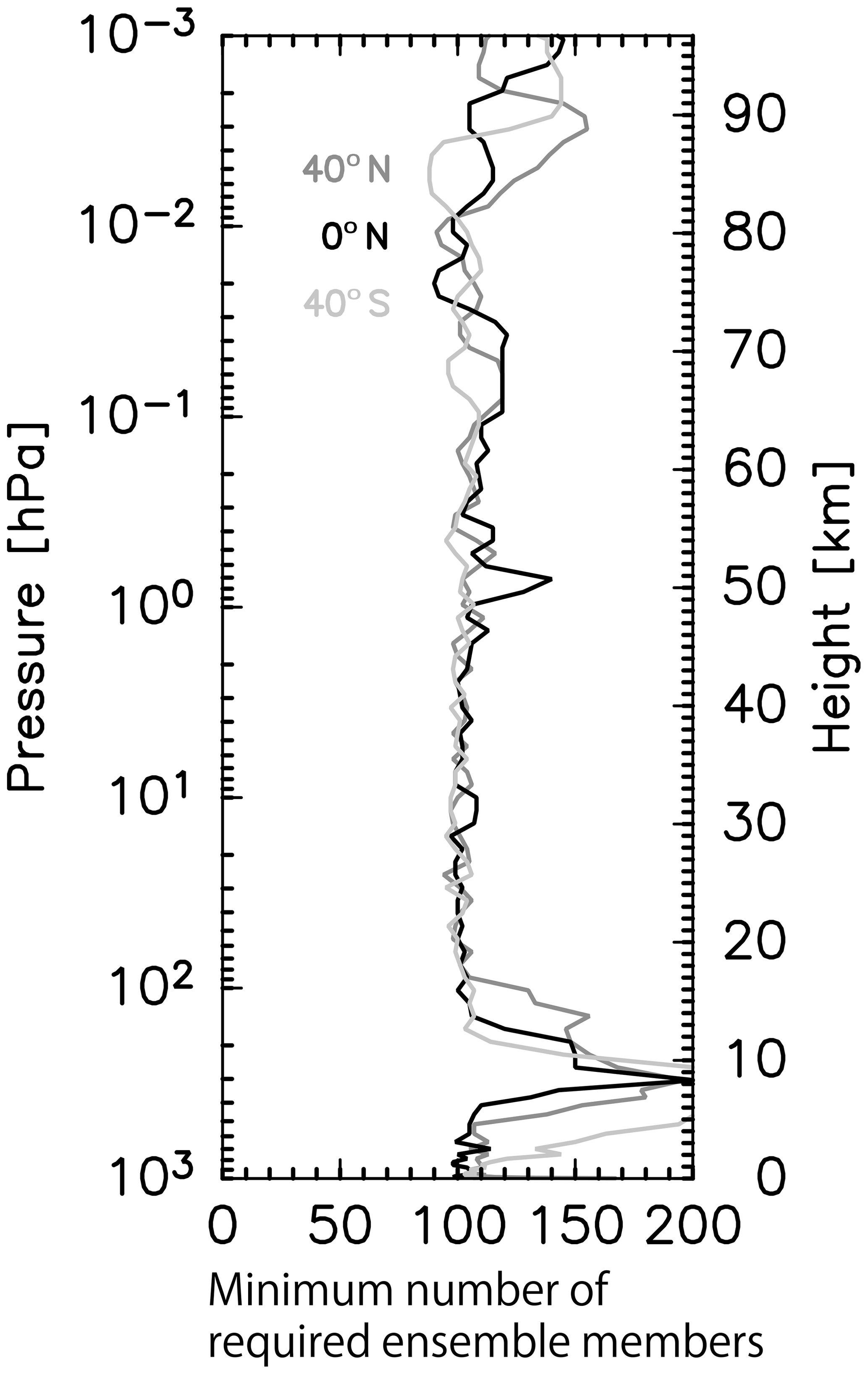
Figure 19 The vertical profiles of the minimum number of required ensemble members that were estimated from the RMS of spurious correlation. The black, dark gray, and light gray curves show the results for the Equator, 40^∘ N, and 40^∘ S, respectively.

Figure 19 shows the minimum optimal number of ensemble members as a function of the height for 40^∘ S, the Equator, and 40^∘ N. Roughly speaking, 100 members are sufficient below 80 km for all displayed latitudes except for 50 km at the Equator. The minimum optimal number of ensemble members above 80 km is larger than 100 and close to 150. From this result, more than 150 ensemble members likely give an optimal estimation of the forecast error covariance for the middle atmosphere. However, it is important to note that even if the number of ensemble members is smaller than 150, using the localization as examined in Sect. 3.3.2 will minimize the effect of the spurious error covariance due to under-sampling, as understood from the good performance of the Ctrl assimilation using 30 ensemble members.

4 Validation of the assimilation

4.1 Comparison with other reanalysis data

This paper gives the first results of the 4D-LETKF applied to the GCM that include the MLT region. Thus, to examine the performance of our assimilation system, the best result obtained from the M200 run among the assimilation experiments is compared with MERRA-2 as one of the standard reanalysis datasets. First, we calculated the spatial correlation of the geopotential height anomaly from the zonal mean as a function of the pressure level and time (Fig. 20). The correlation is higher than 0.9 between ∼900 and ∼1 hPa. The top height with the high correlation varies with time. This time variation may be related to the model predictability, although such a detailed analysis is beyond the scope of the present paper. The reduction of correlation near the ground is likely due to the difference in the resolution of topography.

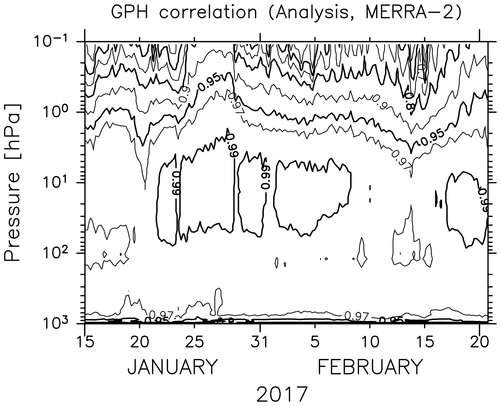
Figure 20 The zonal mean of the spatial correlation of the geopotential height anomaly from the zonal mean between the analysis (M200) and MERRA-2. Contours of 0.5, 0.6, 0.7, 0.8, 0.9, 0.95, 0.97, and 0.99 are shown.

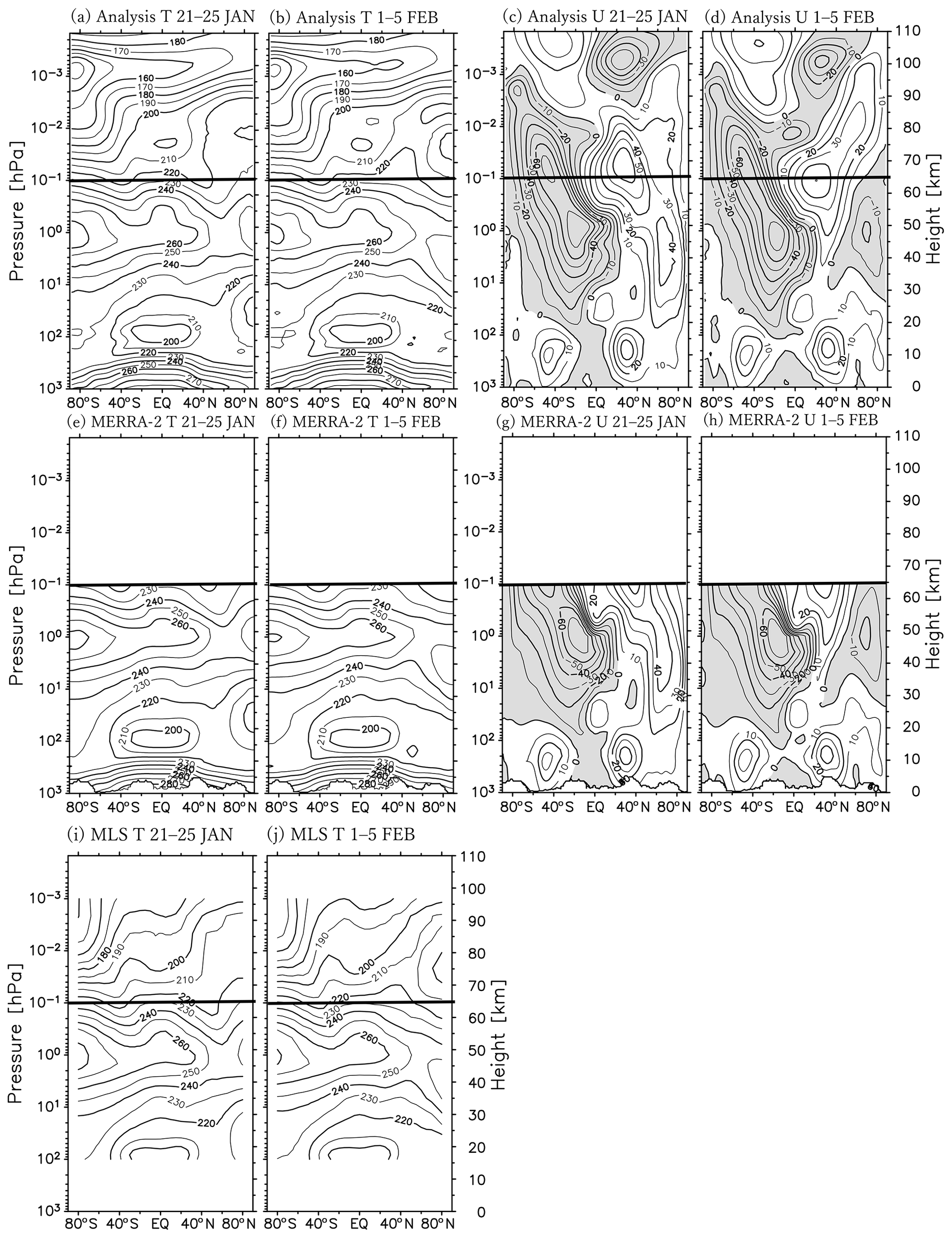
Figure 21 The meridional cross section of the zonal mean temperature (a, b, e, f, i, and j) and zonal wind (c, d, g, and h). Panels (a), (c), (e), (g), and (i) are averaged for the time period of 21–25 January 2017, and panels (b), (d), (f), (h), and (j) are for 1–5 February 2017. Panels (a–d) are the results of the data assimilation (M200), panels (e–h) are the results of the MERRA-2 data, and panels (i) and (j) are the results of the Aura MLS data. The contour intervals are 10 K for (a), (b), (e), (f), (i), and (j) and 10 m s⁻¹ for (c), (d), (g), and (h).

Table 4 Location, radar type, and vertical resolution used for the comparison with the analysis. “MST radar” stands for the mesosphere–stratosphere–troposphere radar.

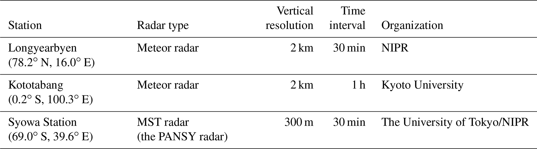
Next, the zonal mean zonal wind and temperature in the latitude–height section from our analysis and MERRA-2 are shown for the time periods before the major warming onset (i.e., 21–25 January) and after (i.e., 1–5 February) (Fig. 21). A thick horizontal bar shows the 0.1 hPa level up to which MERRA-2 pressure level data are provided. The overall structures of the two datasets are similar: the stratopause in the northern polar region is located at a height of ∼ 50 km (∼ 40 km) in the early (later) period. In the Northern Hemisphere, an eastward jet is observed at ∼ 63^∘ N in the wide height range of 20–53 km in the early period. A characteristic westward jet associated with the SSW is observed in the later period in both datasets. The spatial structure and magnitude of the westward jet are both quite similar. In the Southern Hemisphere, a summer westward jet is clearly observed in both sets of data. The poleward tilt with height and a maximum of $\sim -\mathrm{70}$ m s⁻¹ of the jet also accord well. A relatively large difference is observed around 55 km in the equatorial region. The eastward shear with height seems much stronger in MERRA-2 than in our analysis. As the geostrophic balance does not hold in the equatorial region, it may be difficult to reproduce wind by assimilation of only temperature data. This may be the reason for the large discrepancy observed in the equatorial upper stratosphere between the two datasets.

4.2 Comparison with MST and meteor radar observations

The winds obtained from the M200 assimilation experiment are also compared with wind observations by meteor radars at Longyearbyen (78.2^∘ N, 16.0^∘ E; Hall et al., 2002) at 91 km and Kototabang (0.2^∘ S, 100.3^∘ E; Batubara et al., 2011) at 92 km, as well as by the PANSY radar at Syowa Station (69.0^∘ S, 39.6^∘ E) at 85 km. Note that these radar observations were not assimilated and can thus be used for validation as independent reference data. Table 4 gives a brief description of these data. Figure 22 shows the time series of zonal wind and meridional wind observed at each site (black) and corresponding 6-hourly data from our data assimilation analysis (red). A 6 h running mean was made for the time series of the radar data, although the time intervals of original data are much shorter.

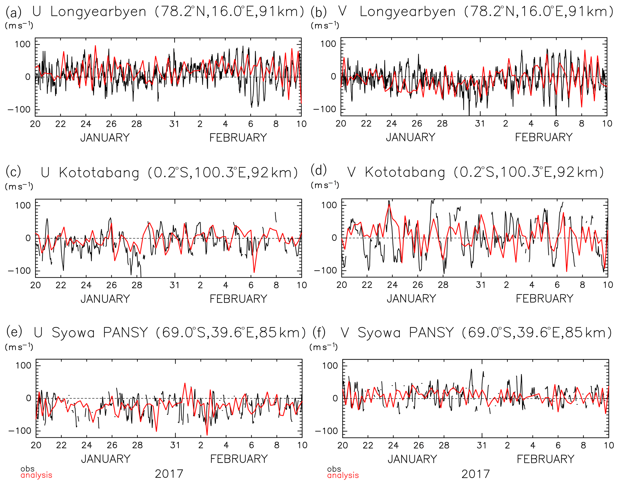
Figure 22 The time series of the zonal (a, c, e) and meridional (b, d, f) wind from 6-hourly analysis (red curves) and from observations (black curves) (a–b) by a meteor radar at Longyearbyen in the Arctic at a height of 91 km, (c–d) by a meteor radar at Kototabang near the Equator at 92 km, and (e–f) by the PANSY radar at Syowa Station in the Antarctic at 85 km. Although the time intervals of the radar observation data are 1 h for meteor radars and 30 min for the PANSY radar, the 6 h running mean time series are plotted.

Strong fluctuations with time-varying amplitudes are observed for both zonal and meridional radar winds for each station. The dominant time period is longer at Kototabang in the equatorial region than that of ∼ 12 h at Longyearbyen in the Arctic. The amplitudes of the meridional wind fluctuations there are larger than those of zonal wind fluctuations at Kototabang. These characteristics are consistent with the wind fluctuations estimated by our assimilation system. However, there are significant differences: the time variation of the amplitudes do not accord well with observations. Differences in the phases of the oscillations between observations and estimations are sometimes small and sometimes large.

In contrast, some consistency is observed for relatively long-period variations (periods longer than several days). At Longyearbyen, the slowly varying zonal wind component is slightly positive before 31 January and significantly positive from 1 to 6 February, while the slowly varying meridional wind tends to be significantly negative in the time period of 28–31 January. At Kototabang, the slowly varying zonal wind tends to be slightly negative before 29 January and almost zero afterward, while the slowly varying meridional wind is almost zero throughout the displayed time period. At Syowa Station, the slowly varying zonal wind tended to be negative from 23 to 30 January and after 2–5 February, while the slowly varying meridional wind tends to be positive from 24 to 31 January.

There are several plausible causes for the discrepancy in short-period variations. First, there may be room to improve the model performance to reproduce such short-period variations. Second, the Aura MLS provides data along a sun-synchronous orbits, and hence fluctuations associated with migrating tides may be hard for it to capture. Third, a large local increment added by the assimilation of the MLS data may cause spurious waves in the model. Fourth, there may be inertia–gravity waves with large amplitudes in the upper mesosphere (e.g., Sato et al., 2017; Shibuya et al., 2017), which cannot be captured with the relatively low-resolution GCM.

5 Summary and concluding remarks

A new advanced data assimilation system employing a 4D-LETKF method for the height region from the surface to the lower thermosphere has been developed using a GCM with a very high top that we called JAGUAR. Observation data from NCEP PREPBUFR and Aura MLS that covered the whole neutral atmosphere up to the lower thermosphere were used for the assimilation. The time period focused on by the present study was 10 January to 28 February 2017. This period includes a major SSW event that occurred on 1 February in the Arctic, for which an international observation campaign for the troposphere, stratosphere, and mesosphere was performed using a radar network.

Before optimizing the parameters of the data assimilation system, the vertical profile of the horizontal dissipation and source intensity of the non-orographic gravity wave parameterization used in JAGUAR were tuned by comparing them to the vertical profiles of gradient winds estimated from the MLS temperature and horizontal winds observed by the PANSY radar. The observation bias in the MLS temperature data was estimated using the SABER temperature data and subsequently corrected.

By performing a series of sensitivity experiments, the best values of the other parameters were obtained for the data assimilation system using 30 ensemble members as a practical assimilation system for the middle atmosphere. The best parameter set is called the Ctrl experiment in Table 1. The optimized value for each parameter in the assimilation of the atmospheric data up to the lower thermosphere was different from those used for the standard model covering the troposphere and stratosphere. There are several possible reasons for these differences: first, the model performance is not very mature for the MLT region. Second, the number of observation data and observable quantities are limited for the MLT region. Third, the dominant disturbances (and dynamics as well) are different from those in the lower atmosphere. Because of the first and second reasons, it is better to take a larger gross error check coefficient in order to include a larger percentage of the observation data. It was shown that the optimal localization length depends on the height: a smaller localization length is better for lower heights. Thus, the best length for the middle of the model altitude range (i.e., 0.1 hPa) was employed in the best parameter set. It was also shown that the inflation factor should be larger than for the standard model, although overly large factors do not give stable ensemble spreads. A shorter assimilation window seemed better for the MLT region, which is probably due to the dominance of short-period disturbances, such as quasi-2 d waves and tides. However, shorter assimilation windows have a problem. The number of available observation data becomes small and the analysis thus tends to be more reflected by the model forecasts that are not as mature as those for the lower atmosphere.

In addition, a minimum optimal number of ensemble members was examined using the results with an assimilation system of 200 ensemble members based on the erroneous ripple of correlation function. The minimum optimal number of ensemble members slightly depends on the height: about 100 members below 80 km and 150 members above. It should be noted, however, that the introduction of the finite localization length to the assimilation may work to avoid spurious correlation at distant locations even with a lower number of ensemble members than the optimal number.

The validity of the data obtained from our assimilation system was examined by comparing the MERRA-2 reanalysis dataset that has the highest top among the currently available reanalysis datasets. The correlation was greater than ∼ 0.95 up to 1 hPa, depending on time. A comparison with radar observations in the upper mesosphere was also performed. The time variation of horizontal winds with periods longer than several days obtained from our assimilation system was consistent with the radar observations. However, the accordance of fluctuations with short wave periods, particularly shorter than 1 d, was not adequate with their slight dependence on the latitude. Nevertheless, the analysis data from our assimilation system will be useful for the study of the detailed dynamical processes in the middle atmosphere, some of which are measured by a limited number of observation instruments. An international observation campaign by an MST radar network has been performed to capture the modulation of the stratosphere and mesosphere, including gravity waves initiated by the major SSW in the Arctic, which encompasses the event that the present study focused on. The low-resolution analysis product from the assimilation system developed in the present study will be used as an initial condition for a high-resolution JAGUAR model to simulate the real atmosphere, including gravity waves.

In future work, we plan to use more observation data in the middle atmosphere for the assimilation. These include satellite data, such as temperature observation data from SABER, radiance data from the SSMIS, and Global Navigation Satellite System (GNSS) radio occultation data, as well as wind data from radars in the mesosphere. We also plan to examine the impact of assimilating these data with observation system simulation experiments using simulation data from a high-resolution GCM. The predictability of the GCM will also be studied in the near future.

Appendix A

Here we show the equivalence of the two methods, namely the calculation of time development after the data assimilation and the 4D data assimilation with the calculation of time development. The case of $j\mathrm{2}=j\mathrm{1}+\mathrm{1}$, that is, x_j2=Mx_j1, is considered. In the first method, the analysis ${\mathit{x}}_{j\mathrm{1}}^{\text{a}}$ and the analysis error covariance matrix ${\mathbf{P}}_{j\mathrm{1}}^{\text{a}}$ at the time step j1 are written using Eqs. (7) and (8):

$$\begin{array}{}\text{(A1)}& {\displaystyle }& {\displaystyle }{\mathit{x}}_{j\mathrm{1}}^{\text{a}}={\mathit{x}}_{j\mathrm{1}}^{\text{f}}+{\mathbf{P}}_{j\mathrm{1}}^{\text{a}}{\mathbf{H}}^{\mathrm{T}}{\mathbf{R}}^{-\mathrm{1}}\left(\mathit{y}-\mathbf{H}{\mathit{x}}_{j\mathrm{1}}^{\text{f}}\right),\text{(A2)}& {\displaystyle }& {\displaystyle }{\mathbf{P}}_{j\mathrm{1}}^{\text{a}}=\left(\mathbf{I}-{\mathbf{P}}_{j\mathrm{1}}^{\text{f}}{\mathbf{H}}^{\mathrm{T}}{\left({\mathbf{HP}}_{j\mathrm{1}}^{\text{f}}{\mathbf{H}}^{\mathrm{T}}+\mathbf{R}\right)}^{-\mathrm{1}}\mathbf{H}\right){\mathbf{P}}_{j\mathrm{1}}^{\text{f}}.\end{array}$$

Using the model forecast matrix M, ${\mathit{x}}_{j\mathrm{2}}^{\text{a}}$ and ${\mathbf{P}}_{j\mathrm{2}}^{\text{a}}$ at the next time step j2 are obtained:

$$\begin{array}{}\text{(A3)}& {\mathit{x}}_{j\mathrm{2}}^{\text{a}}=\mathbf{M}{\mathit{x}}_{j\mathrm{1}}^{\text{a}}=\mathbf{M}{\mathit{x}}_{j\mathrm{1}}^{\text{f}}+{\mathbf{MP}}_{j\mathrm{1}}^{\text{a}}{\mathbf{H}}^{\mathrm{T}}{\mathbf{R}}^{-\mathrm{1}}\left(\mathit{y}-\mathbf{H}{\mathit{x}}_{j\mathrm{1}}^{\text{f}}\right),\end{array}$$

$$\begin{array}{}\text{(A4)}& \begin{array}{rl}{\mathbf{P}}_{j\mathrm{2}}^{\text{a}}& ={\mathbf{MP}}_{j\mathrm{1}}^{\text{a}}{\mathbf{M}}^{\mathrm{T}}\\ & =\mathbf{M}\left(\mathbf{I}-{\mathbf{P}}_{j\mathrm{1}}^{\text{f}}{\mathbf{H}}^{\mathrm{T}}{\left({\mathbf{HP}}_{j\mathrm{1}}^{\text{f}}{\mathbf{H}}^{\mathrm{T}}+\mathbf{R}\right)}^{-\mathrm{1}}\mathbf{H}\right){\mathbf{P}}_{j\mathrm{1}}^{\text{f}}{\mathbf{M}}^{\mathrm{T}}.\end{array}\end{array}$$

In the second method, the analysis ${\mathit{x}}_{j\mathrm{2}}^{\text{a}}$ is written as

$$\begin{array}{}\text{(A5)}& {\mathit{x}}_{j\mathrm{2}}^{\text{a}}={\mathit{x}}_{j\mathrm{2}}^{\text{f}}+{\mathbf{P}}_{j\mathrm{2}}^{\text{a}}{\mathbf{H}}^{{}^{\prime }\mathrm{T}}{\mathbf{R}}^{-\mathrm{1}}\left(\mathit{y}-{\mathbf{H}}^{\prime }{\mathit{x}}_{j\mathrm{2}}^{\text{f}}\right),\end{array}$$

where H^′ is the observation operator at the time step j2 and is related to H:

$$\begin{array}{}\text{(A6)}& {\mathbf{H}}^{\prime }={\mathbf{HM}}^{-\mathrm{1}}.\end{array}$$

By substituting this formula into Eq. (A5), the analysis ${\mathit{x}}_{j\mathrm{2}}^{\text{a}}$ is written as

$$\begin{array}{rl}{\mathit{x}}_{j\mathrm{2}}^{\text{a}}& =\mathbf{M}{\mathit{x}}_{j\mathrm{1}}^{\text{f}}+{\mathbf{P}}_{j\mathrm{2}}^{\text{a}}{\left({\mathbf{HM}}^{-\mathrm{1}}\right)}^{\mathrm{T}}{\mathbf{R}}^{-\mathrm{1}}\left(\mathit{y}-{\mathbf{HM}}^{-\mathrm{1}}{\mathit{x}}_{j\mathrm{2}}^{\text{f}}\right)\\ & =\mathbf{M}{\mathit{x}}_{j\mathrm{1}}^{\text{f}}+{\mathbf{P}}_{j\mathrm{2}}^{\text{a}}{\left({\mathbf{M}}^{-\mathrm{1}}\right)}^{\mathrm{T}}{\mathbf{H}}^{\mathrm{T}}{\mathbf{R}}^{-\mathrm{1}}\left(\mathit{y}-{\mathbf{HM}}^{-\mathrm{1}}{\mathit{x}}_{j\mathrm{2}}^{\text{f}}\right)\\ & =\mathbf{M}{\mathit{x}}_{j\mathrm{1}}^{\text{f}}+{\mathbf{MP}}_{j\mathrm{1}}^{\text{f}}{\mathbf{H}}^{\mathrm{T}}{\mathbf{R}}^{-\mathrm{1}}\left(\mathit{y}-\mathbf{H}{\mathit{x}}_{j\mathrm{1}}^{\text{f}}\right)\\ & =\mathbf{M}{\mathit{x}}_{j\mathrm{1}}^{\text{a}},\end{array}$$

which is identical to Eq. (A3).

Similarly, the analysis error covariance ${\mathbf{P}}_{j\mathrm{2}}^{\text{a}}$ is written as

$$\begin{array}{}\text{(A7)}& {\mathbf{P}}_{j\mathrm{2}}^{\text{a}}=\left(\mathbf{I}-{\mathbf{P}}_{j\mathrm{2}}^{\text{f}}{\mathbf{H}}^{{}^{\prime }\mathrm{T}}{\left({\mathbf{H}}^{\prime }{\mathbf{P}}_{j\mathrm{2}}^{\text{f}}{\mathbf{H}}^{{}^{\prime }\mathrm{T}}+\mathbf{R}\right)}^{-\mathrm{1}}{\mathbf{H}}^{\prime }\right){\mathbf{P}}_{j\mathrm{2}}^{\text{f}},\end{array}$$

which is transformed using Eq. (A6) to

$$\begin{array}{rl}{\mathbf{P}}_{j\mathrm{2}}^{\text{a}}=& \left(\mathbf{I}-{\mathbf{P}}_{j\mathrm{2}}^{\text{f}}{\left({\mathbf{HM}}^{-\mathrm{1}}\right)}^{\mathrm{T}}{\left({\mathbf{HM}}^{-\mathrm{1}}{\mathbf{P}}_{j\mathrm{2}}^{\text{f}}{\left({\mathbf{HM}}^{-\mathrm{1}}\right)}^{\mathrm{T}}+\mathbf{R}\right)}^{-\mathrm{1}}\right.\\ & \left.{\mathbf{HM}}^{-\mathrm{1}}\right){\mathbf{MP}}_{j\mathrm{1}}^{\text{f}}{\mathbf{M}}^{\mathrm{T}}\\ =& \left(\mathbf{I}-{\mathbf{P}}_{j\mathrm{2}}^{\text{f}}{\mathbf{M}}^{-\mathrm{T}}{\mathbf{H}}^{\mathrm{T}}{\left({\mathbf{HM}}^{-\mathrm{1}}{\mathbf{P}}_{j\mathrm{2}}^{\text{f}}{\mathbf{M}}^{-\mathrm{T}}{\mathbf{H}}^{\mathrm{T}}+\mathbf{R}\right)}^{-\mathrm{1}}{\mathbf{HM}}^{-\mathrm{1}}\right)\\ & {\mathbf{MP}}_{j\mathrm{1}}^{\text{f}}{\mathbf{M}}^{\mathrm{T}}\\ =& \left(\mathbf{I}-{\mathbf{MP}}_{j\mathrm{1}}^{\text{f}}{\mathbf{H}}^{\mathrm{T}}{\left({\mathbf{HP}}_{j\mathrm{1}}^{\text{f}}{\mathbf{H}}^{\mathrm{T}}+\mathbf{R}\right)}^{-\mathrm{1}}{\mathbf{HM}}^{-\mathrm{1}}\right){\mathbf{MP}}_{j\mathrm{1}}^{\text{f}}{\mathbf{M}}^{\mathrm{T}}\\ =& \mathbf{M}\left(\mathbf{I}-{\mathbf{P}}_{j\mathrm{1}}^{\text{f}}{\mathbf{H}}^{\mathrm{T}}{\left({\mathbf{HP}}_{j\mathrm{1}}^{\text{f}}{\mathbf{H}}^{\mathrm{T}}+\mathbf{R}\right)}^{-\mathrm{1}}\mathbf{H}\right){\mathbf{P}}_{j\mathrm{1}}^{\text{f}}{\mathbf{M}}^{\mathrm{T}}\\ =& {\mathbf{MP}}_{j\mathrm{1}}^{\text{a}}{\mathbf{M}}^{\mathrm{T}}.\end{array}$$

This is identical to Eq. (A4). These relations can be derived for any j2 other than $j\mathrm{2}=j\mathrm{1}+\mathrm{1}$.