Development of the MIROC-ES2L Earth system model and the evaluation of biogeochemical processes and feedbacks

This article describes the new Earth system model (ESM), the Model for Interdisciplinary Research on Climate, Earth System version 2 for Long-term simulations (MIROC-ES2L), using a state-of-the-art climate model as the physical core. This model embeds a terrestrial biogeochemical component with explicit carbon–nitrogen interaction to account for soil nutrient control on plant growth and the land carbon sink. The model's ocean biogeochemical component is largely updated to simulate the biogeochemical cycles of carbon, nitrogen, phosphorus, iron, and oxygen such that oceanic primary productivity can be controlled by multiple nutrient limitations. The ocean nitrogen cycle is coupled with the land component via river discharge processes, and external inputs of iron from pyrogenic and lithogenic sources are considered. Comparison of a historical simulation with observation studies showed that the model could reproduce the transient global climate change and carbon cycle as well as the observed large-scale spatial patterns of the land carbon cycle and upper-ocean biogeochemistry. The model demonstrated historical human perturbation of the nitrogen cycle through land use and agriculture and simulated the resultant impact on the terrestrial carbon cycle. Sensitivity analyses under preindustrial conditions revealed that the simulated ocean biogeochemistry could be altered regionally (and substantially) by nutrient input from the atmosphere and rivers. Based on an idealized experiment in which CO₂ was prescribed to increase at a rate of 1 % yr⁻¹, the transient climate response (TCR) is estimated to be 1.5 K, i.e., approximately 70 % of that from our previous ESM used in the Coupled Model Intercomparison Project Phase 5 (CMIP5). The cumulative airborne fraction (AF) is also reduced by 15 % because of the intensified land carbon sink, which results in an airborne fraction close to the multimodel mean of the CMIP5 ESMs. The transient climate response to cumulative carbon emissions (TCRE) is 1.3 K EgC⁻¹, i.e., slightly smaller than the average of the CMIP5 ESMs, which suggests that “optimistic” future climate projections will be made by the model. This model and the simulation results contribute to CMIP6. The MIROC-ES2L could further improve our understanding of climate–biogeochemical interaction mechanisms, projections of future environmental changes, and exploration of our future options regarding sustainable development by evolving the processes of climate, biogeochemistry, and human activities in a holistic and interactive manner.

1 Introduction

Originally, global climate projections using climate models were based on simulations using atmosphere-only physical models (Manabe et al., 1965). Numerical climate models evolved through the integration or improvement of component models on ocean circulation (Manabe and Bryan, 1969), land hydrological processes (Sellers et al., 1986), sea ice dynamics (e.g., Meehl and Washington, 1995), and aerosols (e.g., Takemura et al., 2000), most of which focus on physical aspects that affect how climate is formed. Cox et al. (2000) attempted to couple a carbon cycle model and a climate model to investigate the roles of biophysical and biogeochemical (carbon cycle) feedbacks on climate. Their results showed that such interactions are significant in projecting future climate due to processes and feedbacks beyond those incorporated in traditional climate models. Models that incorporate biogeochemical processes, such as that by Cox et al. (2000), are often called Earth system models (ESMs). Currently, the most comprehensive state-of-the-art ESMs include component models of the land and ocean carbon cycle, atmospheric chemistry, dynamic vegetation, and other biogeochemical cycles (e.g., Watanabe et al., 2011; Collins et al., 2011).

Among many processes and possible interactions in the Earth system, the carbon cycle and its feedback on climate remain the focus of simulation studies using ESMs because of the importance of anthropogenic CO₂ as the primary driver for climate change and the complexity of the natural carbon cycle that determines its fate. As ESMs simulate explicit climate–carbon interactions, they can simulate the temporal evolution of the atmospheric CO₂ concentration and the resultant climate change using anthropogenic CO₂ emissions as an input (Friedlingstein et al., 2006, 2014). It is also possible to make climate projections using prescribed CO₂ concentrations, and the diagnosed CO₂ fluxes in the simulations can be used to calculate the level of anthropogenic CO₂ emissions compatible with prescribed CO₂ pathways (Jones et al., 2013). Furthermore, ESM simulations can be diagnosed in terms of the relationship between anthropogenic CO₂ emissions and global temperature rise, i.e., the so-called transient climate response to cumulative carbon emissions (TCRE) (Allen et al., 2009; Matthews et al., 2009). The ESMs of the Coupled Model Intercomparison Project Phase 5 (CMIP5) revealed that the relationship is approximately linear (Gillett et al., 2013), which facilitates the estimation of the total amount of anthropogenic CO₂ emissions to restrict global warming below a specific mitigation target.

The feedback of the carbon cycle on climate is manifested through the regulation of the atmospheric CO₂ concentration, which can be decomposed into two feedback processes. The first process is the carbon cycle response to CO₂ increase. An elevated CO₂ concentration accelerates vegetation growth that intensifies the land carbon sink. Additionally, increased levels of atmospheric CO₂ accelerate CO₂ dissolution into the surface water of the ocean, and the absorbed CO₂ is transported into the deeper ocean via ocean circulation and biological processes. Consequently, an increase in atmospheric CO₂ triggered by external forcing (e.g., anthropogenic emissions) can be partly mitigated by natural CO₂ uptake, forming a negative feedback loop between the atmospheric CO₂ concentration and natural carbon uptake, i.e., the so-called CO₂–carbon feedback (Gregory et al., 2009) or carbon concentration feedback (Boer and Arora et al., 2009). The second feedback process is the carbon cycle response to global warming. Global warming induces the loss of carbon from the land to the atmosphere by accelerating ecosystem respiration (Arora et al., 2013; Todd-Brown et al., 2014; Friedlingstein et al., 2014), while ocean surface warming reduces the solubility of CO₂ in seawater. The intensification of upper-ocean stratification and weakening of the biological pump by global warming also prevent the effective transport of dissolved carbon into the deeper ocean (Frölicher et al., 2015; Yamamoto et al., 2018). Global warming might lead to localized intensification of the natural carbon sink (e.g., lengthening of the growing season and exposure of the ocean surface through melting of sea ice). However, state-of-the-art ESMs have projected global natural carbon loss due to warming, which suggests a positive feedback loop between climate change and natural carbon uptake, i.e., the so-called climate–carbon feedback (Friedlingstein et al., 2006; Arora et al., 2013).

Quantifications of the strength of the carbon cycle feedbacks and their comparison among ESMs were first made by Friedlingstein et al. (2006), who showed that all ESMs agreed with the positive sign of the climate–carbon feedbacks for both land and ocean. The latest comparison using CMIP5 ESMs was made by Arora et al. (2013). They found that the widest spread between the models was in the land carbon response to CO₂ increase, while the second greatest spread was in the land carbon response to warming. Two of the ESMs in their analysis employed explicit carbon–nitrogen (C–N) interactions in the land component for considering the limitation of soil N on land CO₂ uptake, and these two models showed the smallest land carbon response to CO₂ increase. Although it was pointed out later that the lowest response of the two C–N models was not necessarily induced by N limitation (Hajima et al., 2014b), the comparison study by Arora et al. (2013) aroused interest in terrestrial biogeochemical feedbacks other than the carbon cycle. The importance of N limitation on the land carbon sink has also been suggested following simulation studies using offline land models (e.g., Thornton et al., 2007; Sokolov et al., 2008; Zaehle and Friend, 2010) and diagnostic analyses using the simulation output of ESMs (e.g., Wieder et al., 2015).

Compared with land, the oceans showed better agreement among the CMIP5 ESMs (Arora et al., 2013) in terms of the strength of both CO₂–carbon and climate–carbon feedbacks. However, the ESMs showed substantial discrepancies in the spatiotemporal patterns of ocean CO₂ uptake, even in historical simulations. In particular, in the Southern Ocean, although the models indicated dominance of the region in relation to anthropogenic carbon uptake (Frölicher et al., 2015), the seasonality of the atmosphere–ocean CO₂ flux and the cumulative values in that region showed divergent patterns among the models (Anav et al., 2013; Frölicher et al., 2015; Kessler and Tjiputra, 2016).

The ecological response of the ocean in ESMs remains far from certain. A benchmark study by Anav et al. (2013) revealed that all CMIP5 ESMs underestimate net primary productivity (NPP) in the high latitudes of the Northern Hemisphere, where seawater temperature and N availability likely limit primary production (e.g., Moore et al., 2013). They also found that most models overestimate NPP in the Southern Hemisphere high latitudes, where the nutrient supply is sufficient because of strong upwelling but the iron supply is limited (Moore et al., 2013). Globally, the CMIP5 ESMs simulate NPP with different magnitudes, even in preindustrial conditions, and the global NPP response among the models to past and future climate change is largely divergent (Laufkötter et al., 2015), as is the sinking particle flux (Fu et al., 2016). Although such problems regarding oceanic NPP might be partly attributable to an inaccurate reproduction of oceanic physical fields by the models (Frölicher et al., 2015; Laufkötter et al., 2015), it is critical in simulations to accurately reproduce the relative abundances of nutrients in the euphotic zone and their availability to microorganisms. In particular, nutrients in the upper ocean are sustained by upwelling from the deeper ocean and inputs from external sources. Some studies suggest that nutrient availability to marine ecosystems could decline in the future through the reduction of nutrient upwelling because of intensified stratification (e.g., Ono et al., 2008; Whitney et al., 2013; Yasunaka et al., 2016). Conversely, other studies suggest that nutrient supply through atmospheric deposition and river discharge processes could be amplified in the future because of human activities (Gruber and Galloway, 2008; Mahowald et al., 2009) unless robust mitigation policies are adopted. Thus, to project the effects of biogeochemical feedback on climate, it is necessary to consider the response of ecological processes to changing nutrient inputs as well as the physical response.

On the basis of the above, we previously reviewed the CMIP5 exercises and discussed the perspective for new ESM development (Hajima et al., 2014a). In our ESM development, we prioritized the incorporation of explicit C–N interaction in the land biogeochemical component. The terrestrial nitrogen cycle regulates the carbon cycle by modulating soil nutrient availability to plants, regulating leaf N concentration and photosynthetic capacity, and changing the C:N ratio in plants and soils. In particular, CO₂ stimulation of plant growth (the so-called CO₂ fertilization effect) is the main driver of terrestrial CO₂–carbon feedback, while N limitation on plant growth might regulate the feedback strength (Arora et al., 2013; Hajima et al., 2014a, b). Thus, consideration of C–N coupling in the terrestrial ecosystem in an ESM will enable change in the land carbon sink capacity following a change in N dynamics induced by human perturbation (e.g., fertilizers) and/or atmospheric N deposition.

For the ocean, the biogeochemical component in our previous model (MIROC-ESM; Watanabe et al., 2011) was unchanged from that used for the first stage of the Coupled Climate Carbon Cycle Model Intercomparison Project (C4MIP; Friedlingstein et al., 2006; Yoshikawa et al., 2008). The ocean component simulated C and N cycles only, using simple parameterizations of ocean ecosystem dynamics with four types of N tracer and five C tracers (Watanabe et al., 2011) with fixed C:N ratios of the organic components. Furthermore, the ocean N cycle in the model was isolated from other subsystems; i.e., there was no N input into the ocean (e.g., biological N fixation, atmospheric N deposition, and riverine N input) or flux out of the system (e.g., outgassing and sedimentation). To account for changing inputs of N nutrients into the ocean in the simulations, we gave second priority to the coupling of the ocean N cycle to other subsystems by incorporating N exchange processes between the ocean and other components in the new ESM. The ocean N fixer (i.e., diazotrophs) can be strongly regulated by P availability (Shiozaki et al., 2018); therefore, inclusion of the ocean P cycle should be adopted together with improvement of the N cycle. Additionally, as the denitrification process is strongly regulated by the level of oxygen in seawater, it was also decided to include the oxygen cycle in the new model. Inclusion of the oxygen cycle provides potential to project future oceanic deoxygenation that is likely to threaten the habitable zone of marine ecosystems driven by changes in oxygen solubility, mixing, circulation, and respiration due to global warming (Oschlies et al., 2018; Yamamoto et al., 2015).

The third priority in developing a new ESM was the incorporation of Fe cycle processes. Fe is an essential micronutrient for phytoplankton. Thus, any model lacking consideration of the Fe cycle potentially overestimates primary productivity, especially in regions in which the subsurface macronutrient supply is enhanced but Fe availability is limited, e.g., the main oceanic upwelling “high-nutrient, low-chlorophyll” (HNLC) regions (Martin and Gordon, 1988; Moore et al., 2013). Similar to the N cycle, the ocean Fe cycle is also an open system. One of its main external sources is dissolved Fe from continental margins and from hydrothermal vents along mid-ocean ridges (Tagliabue et al., 2017). Thus, the continental and hydrothermal Fe supply is important in terms of determining the background Fe concentration in seawater. Additionally, the ocean Fe cycle is also connected to the land through the atmosphere (Jickells et al., 2005; Mahowald et al., 2009; Ito et al., 2019a). Fe-containing aerosols are emitted from dry land surfaces, open biomass burning, and fossil fuel combustion, and they are delivered to marine ecosystems via dry and wet deposition processes. These processes have been perturbed by climate change, land use change (LUC), and air pollution (Jickells et al., 2005; Mahowald et al., 2009; Ito et al., 2019a). Thus, consideration of atmospheric Fe deposition, in particular, is necessary to reflect the anthropogenic impact on future marine ecosystem dynamics via Fe cycle processes.

Here, we present a description of a new ESM, the Model for Interdisciplinary Research on Climate, Earth System version 2 for Long-term simulations (MIROC-ESL2), which considers explicit carbon and nitrogen cycles for land and carbon, nitrogen, iron, phosphate, and oxygen cycles for the ocean. In the model, the biogeochemical components are coupled interactively with physical climate components, enabling consideration of climate–biogeochemical feedbacks. The model description and experimental settings are presented in Sect. 2. The basic performance of the model, evaluated by executing a historical simulation and comparison of the results with observation-based studies, is presented in Sect. 3.1. To evaluate the sensitivity of the biogeochemical processes, experiments for sensitivity analysis were performed and the results compared with existing studies. In particular, the global temperature response to cumulative anthropogenic CO₂ emissions in the new model was quantified and compared with that of the CMIP5 ESMs to characterize the general features of the new model in relation to existing ESMs. The results of the sensitivity analyses are presented in Sect. 3.2. Finally, a summary and perspectives obtained from this study are offered in Sect. 4.

2 Methods

2.1 Model configurations

To comprehensively describe the MIROC-ES2L structure (Fig. 1), we first present the physical core of MIROC5.2, which is an updated version of MIROC5 used in CMIP5. Only a brief summary is presented here because a detailed description of the modeling of MIROC5 can be found in Watanabe et al. (2010), and an account of a simulation study performed by MIROC5.2 can be found in Tatebe et al. (2018). Additionally, a description of MIROC6, which shares almost the same structure and many of the characteristics of MIROC5.2 except for the atmospheric spatial resolution and cumulus treatments, can be found in Tatebe et al. (2019). In this paper, a description of the land and ocean biogeochemistry is presented in detail because those two components represent the main modifications from the previous version of the ESM (i.e., MIROC-ESM; Watanabe et al., 2011).

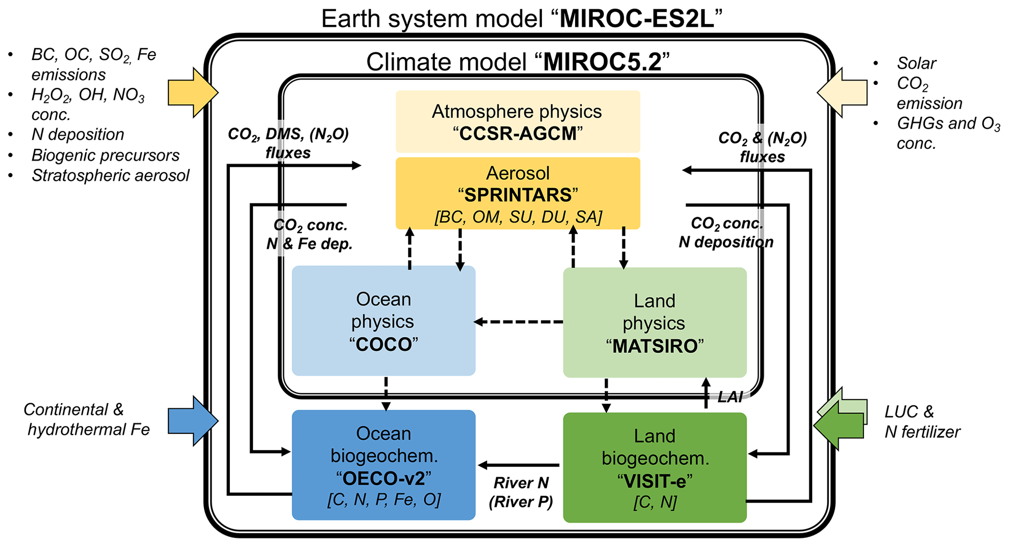
Figure 1 Schematic of component models in the new MIROC-ES2L Earth system model, the biogeochemical and biophysical interactions, and external forcing. The physical core of the model is MIROC5.2, which comprises an atmospheric climate model (CCSR-NIES AGCM or MIROC-AGCM) with an aerosol module (SPRINTARS), an ocean physical model (COCO) with a sea ice model, and a land physical model (MATSIRO) with a river submodel. The land biogeochemistry component (VISIT-e) simulates carbon and nitrogen cycles with an LUC submodel, and the ocean biogeochemistry component (OECO) simulates the cycles of carbon, nitrogen, iron, phosphorus, and oxygen. Color-boxed arrows indicate external forcing. Solid (dashed) black arrows represent biogeochemical (physical) variables exchanged between the component models (the exchanges of physical variables are almost the same as in MIROC-ESM; see Table 1 of Watanabe et al., 2011). Variables in square brackets represent the prognostic biogeochemical cycles and aerosol species (black carbon, BC; organic matter, OM; sulfate (including precursors), SU; dust, DU; sea salt, SA). The names of exchanged variables within parentheses are diagnosed variables, i.e., ocean–land riverine P flux diagnosed from the N flux and simulated land and ocean N₂O fluxes used for diagnostic purposes.

2.1.1 Physical core

The MIROC5.2 physical core comprises component models of the atmosphere, ocean, and land. The atmospheric model is based on a spectral dynamical core originally named the Center for Climate System Research–National Institute for Environmental Studies atmospheric general circulation model (CCSR-NIES AGCM; Numaguti et al., 1997), which is interactively coupled with an aerosol component model called the Spectral Radiation-Transport Model for Aerosol Species (SPRINTARS; Takemura et al., 2000, 2005). For the ocean, the CCSR Ocean Component (COCO) model (Hasumi, 2006) is used in conjunction with a sea ice component model. For land, the Minimal Advanced Treatments of Surface Interaction and Runoff (MATSIRO) model (Takata et al., 2003) is coupled to simulate the atmosphere–land boundary conditions and freshwater input into the ocean. Considering the application possibility of the ESM to long-term climate simulations of more than hundreds of years, e.g., paleoclimate studies (Ohgaito et al., 2013; Yamamoto et al., 2019), the horizontal resolution of the atmosphere is set to have T42 spectral truncation, which is approximately 2.8^∘ intervals for latitude and longitude. The vertical resolution is 40 layers up to 3 hPa with a hybrid σ–p coordinate, as in MIROC5. The horizontal coordination for the ocean is changed from the bipolar system employed in MIROC5 to a tripolar system in MIROC5.2 that is divided horizontally into 360×256 grids. (To the south of 63^∘ N, the longitudinal grid spacing is 1^∘ and the meridional spacing becomes fine near the Equator. In the central Arctic Ocean, the grid spacing is finer than 1^∘ because of the tripolar system.) The vertical levels increase from 44 to 62 with a hybrid σ–z coordinate system. For land, the same horizontal resolution as used for the atmosphere is employed; the vertical soil structure of the model has six layers down to the depth of 14 m. Subgrid fractions for two land use types (agriculture plus managed pasture and others) are considered for the physical processes.

For the AGCM, the schemes used for the dynamical core, radiation, cumulus convection, and cloud microphysics are mostly the same as in MIROC5; the major update of processes mainly concerns the aerosol module. The version used here treats atmospheric organic matter (OM) as one of the prognostic variables, and emissions of primary OM and precursors for secondary OM are diagnosed in the component. For land, the scheme for subgrid snow distribution is replaced by one incorporating a physically based approach (Nitta et al., 2014; Tatebe et al., 2019), and wetland formed temporarily in the snowmelt season is newly considered to reduce the warm bias in temperature in the European region during spring–summer (Nitta et al., 2017; Tatebe et al., 2019). The ocean and sea ice components are mostly the same as in MIROC5.

2.1.2 Land biogeochemical processes

The model of the land ecosystem–biogeochemistry component in MIROC-ES2L is the Vegetation Integrative SImulator for Trace gases model (VISIT; Ito and Inatomi, 2012a). This model simulates carbon and nitrogen dynamics on land (schematics for the carbon cycle can be found in Ito and Oikawa, 2002, and for the nitrogen cycle in Supplement Fig. S1). It has been used for ecological studies of the site–global scale (e.g., Ito and Inatomi, 2012b), impact assessments of climate change (e.g., Warszawski et al., 2013; Ito et al., 2016a, b), CO₂ flux inversion studies (e.g., Maksyutov et al., 2013; Niwa et al., 2017), and contemporary assessments of CO₂, CH₄, and N₂O emissions in the Global Carbon Projects (Le Quéré et al., 2016; Saunois et al., 2016; Tian et al., 2018). The early version of the model (Sim-CYCLE; Ito and Oikawa, 2002) was actually used as the land carbon cycle component in the first stage of the C4MIP project (Friedlingstein et al., 2006; Yoshikawa et al., 2008). The model covers major processes relevant to the global carbon cycle. Photosynthesis or gross primary productivity (GPP) is simulated based on the Monsi–Saeki theory (Monsi and Saeki, 1953), which provides a conventional scheme to simulate leaf-level photosynthesis in a semiempirical manner and for upscaling to canopy-level primary productivity. The allocation of photosynthate between carbon pools in vegetation (e.g., leaf, stem, and root) is regulated dynamically following phenological stages. The transfer of vegetation carbon into litter–soil pools is simulated using constant turnover rates, and in deciduous forests, seasonal leaf shedding occurs at the end of the growing period. The model focuses on biogeochemical processes and it does not explicitly simulate dynamic change in vegetation composition; therefore, the biogeochemical processes are simulated under a fixed biome distribution (Supplement Fig. S2). The carbon stored in litter (i.e., foliage, stem, and root litter) and humus (i.e., active, slow, and passive) pools is decomposed and released as CO₂ into the atmosphere under the influence of soil water and temperature. Further details on the carbon cycle processes in the model can be found in Ito and Oikawa (2002).

For the nitrogen cycle, the model considers two major nitrogen influxes to the ecosystem: biological nitrogen fixation (BNF) simulated based on the scheme of Cleveland et al. (1999) and external nitrogen sources such as fertilizer and atmospheric nitrogen deposition, which are prescribed in the forcing data. The fluxes of nitrogen out of the land ecosystem are simulated through N₂ and N₂O production during nitrification and denitrification in soils based on the scheme of Parton et al. (1996), leaching of inorganic nitrogen from soils, which is affected by the amount of soil nitrate and runoff rate, and NH₃ volatilization from soils (Lin et al., 2000; Thornley, 1998). Within the vegetation–soil system, organic nitrogen in the soil is supplied from litter fall, whereas inorganic nitrogen is released through soil decomposition processes (soil mineralization) and stored as two chemical forms (${\mathrm{NO}}_{\mathrm{3}}^{-}$ and ${\mathrm{NH}}_{\mathrm{4}}^{+}$). Inorganic nitrogen is taken up by plants, allocated to two vegetation pools (canopy and structural pools), and immobilized into a microbe pool. Finally, mineral nitrogen is lost via biotic–abiotic processes as mentioned above.

Although the original land component model covers most major carbon–nitrogen processes, for the purposes of inclusion in the new ESM and making fully coupled climate–carbon–nitrogen projections, the land model was modified for this study (hereafter, the modified version is called VISIT-e). First, the modified model represents the close interaction between carbon and nitrogen in plants. This is because the original model has only a loose interaction between these two cycles, and thus it cannot precisely predict the nitrogen limitation on primary productivity. To achieve this, the photosynthetic capacity in VISIT-e is modified to be controlled by the amount of nitrogen in leaves (leaf nitrogen concentration), which is determined by the balance between the nitrogen demand of plants and potential supply from the soil. Thus, if sufficient inorganic nitrogen is not available for plants, the leaf nitrogen concentration is gradually lowered, which reduces photosynthetic capacity and the plant production rate. This process is required to simulate the observed downregulation in elevated CO₂ experiments (e.g., Norby et al., 2010; Zaehle et al., 2014). Other modifications regarding the nitrogen cycle are described in Appendix A.

Second, although the original VISIT incorporates LUC and associated CO₂ emission processes, to take full advantage of the latest LUC forcing dataset (Land-Use Harmonization 2; Ma et al., 2019), additional LUC-related processes have been newly introduced in VISIT-e. The model assumes five types of land cover (each represented on a separate tile) in each land grid box (i.e., primary vegetation, secondary vegetation, urban, cropland, and pasture) with the same structure of carbon–nitrogen pools. All processes are calculated separately for each tile (i.e., no lateral interaction), and then the variables in the tile are summed after weighting by the areal fraction of each land use type. The LUC impact is modeled assuming two types of land use impact on the biogeochemistry. The first impact considers status-driven LUC processes, which affect land biogeochemistry even when the areal fractions of the tiles are fixed. For example, even when a simulation is conducted with fixed areal fractions (e.g., a spin-up run under 1850 conditions), crop harvesting, nitrogen fixation by N-fixing crops, and the decay of OM in product pools occur. The second type of land use impact includes transition-driven processes that happen only when areal changes occur among the tiles. For example, when an areal fraction is changed within a year (e.g., conversion of forest to urban land use), carbon and nitrogen in the harvested biomass are translocated between product pools. When cropland is abandoned and the area is reclassified as secondary forest, the apparent mean mass density of secondary forest is first diluted because of the increase in the less vegetated area, and then secondary forest starts regrowth toward a new stabilization state. A further detailed description of LUC modeling is given in Appendix A.

The land ecosystem component runs with a daily time step in the ESM. It has fixed spatial distribution patterns of 12 vegetation categories (see Supplement Fig. S2), and the land biogeochemistry is affected by daily averaged atmospheric conditions (CO₂ concentration, downward shortwave radiation, air temperature, and air pressure) and land abiotic conditions (soil water, soil temperature, and runoff rate as the base flow) simulated by the physical core of the ESM. In turn, daily averaged land variables simulated by VISIT-e are used by other components of the ESM (Fig. 1). For example, the simulated leaf area index (LAI) is referenced in the physical core of the model to simulate physical dynamics on the land surface (e.g., evapotranspiration, albedo, and surface roughness). Furthermore, the rate of net atmosphere–land CO₂ flux is used in the calculation of the atmospheric CO₂ concentration, and inorganic N leached from the soil is transported by rivers and subsequently used as an input of N nutrients to the ocean ecosystem. The chemical state of N in rivers is assumed conserved during transportation, and biogeochemical processes such as outgassing or sedimentation in freshwater systems are neglected in the present model. Additionally, although the model can simulate terrestrial carbon loss by erosion and dissolution of organic carbon, these processes are not activated to close the global mass conservation of carbon and nitrogen. Finally, although N₂O and NH₃ emissions are simulated, the emission fluxes are considered only for diagnostic purposes and they do not produce any change in the atmospheric radiation balance or air quality.

2.1.3 Ocean biogeochemical processes

The new ocean biogeochemical component model OECO2 (see Supplement Fig. S3 for a schematic) is a nutrient–phytoplankton–zooplankton–detritus-type model that is an extension of the previous model (Watanabe et al., 2011). Although only an overview of OECO2 is presented here, a detailed description can be found in Appendix B.

In OECO2, ocean biogeochemical dynamics are simulated with 13 biogeochemical tracers. Three of them are associated with cycles of macronutrients (nitrate and phosphate) and a micronutrient (dissolved Fe). The model has four organic tracers of “ordinary” nondiazotrophic phytoplankton, diazotrophic phytoplankton (nitrogen fixer), zooplankton, and particulate detritus. All OM in these four tracers is assumed to have an identical nutrient, oxygen, and micronutrient iron composition following the Redfield ratio of $\mathrm{C}:\mathrm{N}:\mathrm{P}:\mathrm{O}$ = $\mathrm{106}:\mathrm{16}:\mathrm{1}:\mathrm{138}$ (Takahashi et al., 1985) and C:Fe = $\mathrm{150}:{\mathrm{10}}^{-\mathrm{3}}$ (Gregg et al., 2003). Four other tracers are associated with carbon and/or calcium, i.e., dissolved inorganic carbon (DIC), total alkalinity, calcium, and calcium carbonate. The two other tracers are oxygen and nitrous oxide.

The nitrogen cycle in OECO2 is similar to that in the previous version (Yoshikawa et al., 2008; Watanabe et al., 2011), except the new model accounts for nitrogen influxes such as nitrogen deposition from the atmosphere (as external forcing), input of inorganic nitrogen from land via rivers, and BNF by diazotrophic phytoplankton (Fig. 1). Additionally, denitrification is also modeled as the dominant process of oceanic nitrogen loss, with an explicit distinction between the gaseous forms of N₂O and N₂ (see below for nitrogen fixation and denitrification processes). Loss of nitrogen through the sedimentation process is also considered. The phosphorus cycle is newly embedded in the model to represent strong phosphorous limitation on the growth of diazotrophic phytoplankton. The structure of the phosphorus cycle is generally similar to that of nitrogen except in two respects: (1) the riverine input of phosphate is the only process that introduces phosphorus into the ocean, and (2) there is no process of outgassing from the ocean, unlike the denitrification process in the nitrogen cycle. As the land ecosystem model cannot simulate the phosphorus cycle, the flux of phosphorous from rivers is diagnosed from the nitrogen flux, assuming that the phosphate brought to the river mouth satisfies the N:P ratio of 16:1, similar to the Redfield ratio.

The structure of the ocean iron cycle is also similar to that of nitrogen, except the following processes are modeled as iron input into the ocean. Two major sources of iron deposition from the atmosphere are included in the new model: lithogenic and pyrogenic sources. Mineral dust emission is diagnosed by the aerosol component module, depending on the near-surface wind speed, soil dryness, and bare ground cover, while iron emitted from biomass burning and the consumption of fossil fuel and biofuel follows external forcing. The latter emission dataset used in this study is shown in Supplement Fig. S4. The iron emissions from pyrogenic sources are estimated based on the iron content and emissions of particulate matter (Ito et al., 2018). A shift from coal to oil combustion is considered in relation to shipping (Fletcher, 1997; Endresen et al., 2007). The iron content of mineral dust is prescribed at 3.5 % (Duce and Tindale, 1991). The iron deposition from biomass burning is calculated from black carbon (BC) deposition and a ratio of 0.04 gFe gBC⁻¹ in fine particles at emission (Ito, 2011). The emission, transportation, and deposition processes are simulated explicitly by the atmospheric aerosol component. The iron from different sources has different solubility in seawater, and thus different amounts of iron are available for phytoplankton. The solubility of iron is prescribed at 79 % for oil combustion, 11 % for coal combustion, and 18 % for biomass burning (Ito, 2013). The solubility of iron for mineral dust is prescribed at 2 % (Jickells et al., 2005).

In addition to the Fe input from the atmosphere, recent studies suggest contributions of Fe supply from sediment and hydrothermal vents to ecosystem activities (Tagliabue et al., 2017). The contributions of these two natural Fe sources to the determination of the atmospheric CO₂ concentration and export production are similar to or greater than that of dust (Tagliabue et al., 2014). Therefore, these three Fe sources are also considered in the new ESM (Appendix B).

Ocean ecosystem dynamics are simulated based on the nutrient cycles of nitrate, phosphorous, and iron. The nutrient concentration, in conjunction with the controls of seawater temperature and the availability of light, regulates the primary productivity of the two types of phytoplankton. The model assumes that diazotrophic phytoplankton can prosper in regions in which phosphate is available but the nitrate concentration is small (<0.05 µmol L⁻¹). In the model, zooplankton is assumed to be independent of abiotic conditions (e.g., seawater temperature) and dependent on biotic conditions (phytoplankton and zooplankton concentrations), as in the previous model. The denitrification process is modeled to occur only in suboxic waters (<5 µmol L⁻¹) (Schmittner et al., 2008), and it is suppressed in water with a low nitrate concentration (<1 µmol L⁻¹). Detritus contains nitrate, phosphorus, iron, and carbon, most of which is remineralized while sinking downward. The detritus that reaches the ocean floor is removed from the system; however, a fraction of OM in the sediment is assumed to return to the bottom layer of the water column at a constant rate in each location (Kobayashi and Oka, 2018).

The ocean carbon cycle is formed by atmosphere–ocean CO₂ exchange, inorganic carbon chemistry, OM dynamics driven by marine ecosystem activities, and transportation and reallocation processes of ocean carbon within the interior. The formulations of atmosphere–ocean gas exchange, carbon chemistry, and related parameters follow protocols from the Ocean Model Intercomparison Project (OMIP; Orr et al., 2017). The production of DIC and total alkalinity is controlled by changes in inorganic nutrients and CaCO₃, following Keller et al. (2012).

Finally, the flux of dimethyl sulfide (DMS) from the ocean, which is produced by plankton and is a precursor of atmospheric sulfate aerosols, is diagnosed in the original aerosol module from the surface downward shortwave radiation flux. In MIROC-ES2L, this emission scheme is modified and the flux is calculated from the sea surface DMS concentration that is diagnosed from the simulated surface water chlorophyll concentrations and the corresponding mixed-layer depth (Appendix B). In the present model, this is the only pathway via which ocean biogeochemistry affects climate if the model is driven by a prescribed CO₂ concentration (Fig. 1). This modification of the DMS emission scheme increases the sulfate aerosol amount, particularly over high-latitude oceans during winter and in regions in which high surface wind speed occurs. The solar irradiance of the surface decreases in such regions; however, this effect is not sufficiently significant to change the mean physical climate states.

2.2 Experiments, forcing, and metrics

2.2.1 Experiments and forcing

To evaluate the performance and sensitivities of MIROC-ES2L, we conducted four groups of experiments comprising 11 experiments in total (Tables 1 and 2). The first group was a control run that comprised two types of experiments: a normal control run (CTL) in which the external forcing was set to preindustrial conditions and an alternative control run (CTL-D) used for sensitivity analysis of the ocean biogeochemistry, which is described later.

The second group, used for historical simulations, comprised three types of experiments during the period 1850–2014. All three experiments were driven by the Coupled Model Intercomparison Project Phase 6 (Eyring et al., 2016) official forcing datasets (version 6.2.1; details on the forcing datasets used in the simulations are summarized in Appendix C), and the CO₂ concentration was prescribed in the simulations (i.e., so-called concentration-driven experiments). The first comprised a conventional historical simulation (HIST), and the simulation result is used for direct comparison with observation-based studies to evaluate model performance. The second was a special experiment named HIST-NOLUC, which was designed to evaluate the impact of LUC on the climate and biogeochemistry. In this experiment, land use and agricultural management (fertilizer application) were fixed at preindustrial levels. This experimental configuration is the same as the LUMIP experiment in CMIP6 named land-noLu (Lawrence et al., 2016). The third experiment (HIST-BGC) was the same as HIST, except that the CO₂ increase only affects the carbon cycle processes (named in C4MIP of CMIP6 as hist-bgc; Jones et al., 2016). Thus, there was no CO₂-induced global warming in the experiment.

The third experimental group was used to evaluate the climate and carbon cycle feedbacks. This group comprised three types of idealized experiments, following experimental designs proposed by Eyring et al. (2016) and Jones et al. (2016). In the three experiments, the CO₂ concentration was prescribed to increase at the rate of 1.0 % per year from the preindustrial state throughout the 140-year period (i.e., the concentration finally reached a value of approximately 1140 ppmv), while other external forcing was maintained at the preindustrial condition. The three experiments were configured as follows: (1) 1PPY was a normal experiment in which both climate and biogeochemical processes respond to the CO₂ increase; (2) 1PPY-BGC was the same as 1PPY but the prescribed CO₂ increase affects only the carbon cycle processes; and (3) 1PPY-RAD was the same as 1PPY but the CO₂ increase affects only atmospheric radiation processes. In 1PPY-BGC, carbon cycle processes respond to the CO₂ increase without CO₂-induced global warming; thus, the result of this simulation is used to quantify the CO₂–carbon feedback. In 1PPY-RAD, as there is no direct CO₂ stimulation on the carbon cycle, climate change is the only cause of carbon cycle variation relative to the preindustrial control (CTL). Thus, this simulation result is used to evaluate the climate–carbon feedback (Arora et al., 2013; Schwinger et al., 2014).

The final group comprised a set of experiments to evaluate ocean biogeochemistry, focusing mainly on the processes newly introduced in MIROC-ES2L. This group comprised three types of experiments. The first experiment (NO-NR) was configured similarly to the CTL run, except the ocean component did not receive any riverine N input. Through this experiment, the impact of riverine N on ocean biogeochemistry could be evaluated. The second experiment (NO-NRD) was the same as NO-NR, except atmospheric N deposition additionally had no effect on ocean biogeochemistry. By evaluating the difference between NO-NR and NO-NRD, the impact of nitrogen deposition on ocean biogeochemistry could be evaluated. The final experiment (NO-FD) was configured with atmospheric Fe deposition onto the ocean surface switched off. To detect slight signals of ocean biogeochemistry arising from switching off the three processes (i.e., riverine N, N deposition, and Fe deposition), it was necessary to maintain consistency in the ocean physical fields between these experiments because a slight difference in the ocean physical fields produces perturbation on ocean biogeochemistry. In MIROC-ES2L, the ocean DMS emissions represent the feedback process of ocean biogeochemistry on the atmospheric physical processes; thus, biogeochemical change induced by the switching-off manipulations must change the DMS emission, which leads to inconsistency in the physical fields between the experiments. To avoid this occurrence, the DMS emission scheme in all three experiments was reverted to that used in the original aerosol component model, which is independent of the ocean ecosystem state (Appendix B). Similarly, the special control run (CTL-D), which was based on CTL, also had the DMS emission scheme changed to the same as NO-NR, NO-NRD, and NO-FD.

To conduct the experiments described above, preindustrial spin-up was performed in advance. Land and ocean biogeochemical components were decoupled from the ESM, and the spin-up run was conducted for 3000 years for the ocean component and 30 000 years for land by prescribing model-derived physical fields and other external forcing for the component models. In the final phase of the spin-up procedure, continuous spin-up, forced by the 1850-year condition of CMIP6 forcing, was performed for the entire system for 2483 years (Supplement Fig. S5). All the experiments listed in Table 1 were initiated from the final condition of this spin-up procedure.

Table 1 Summary of experimental details.

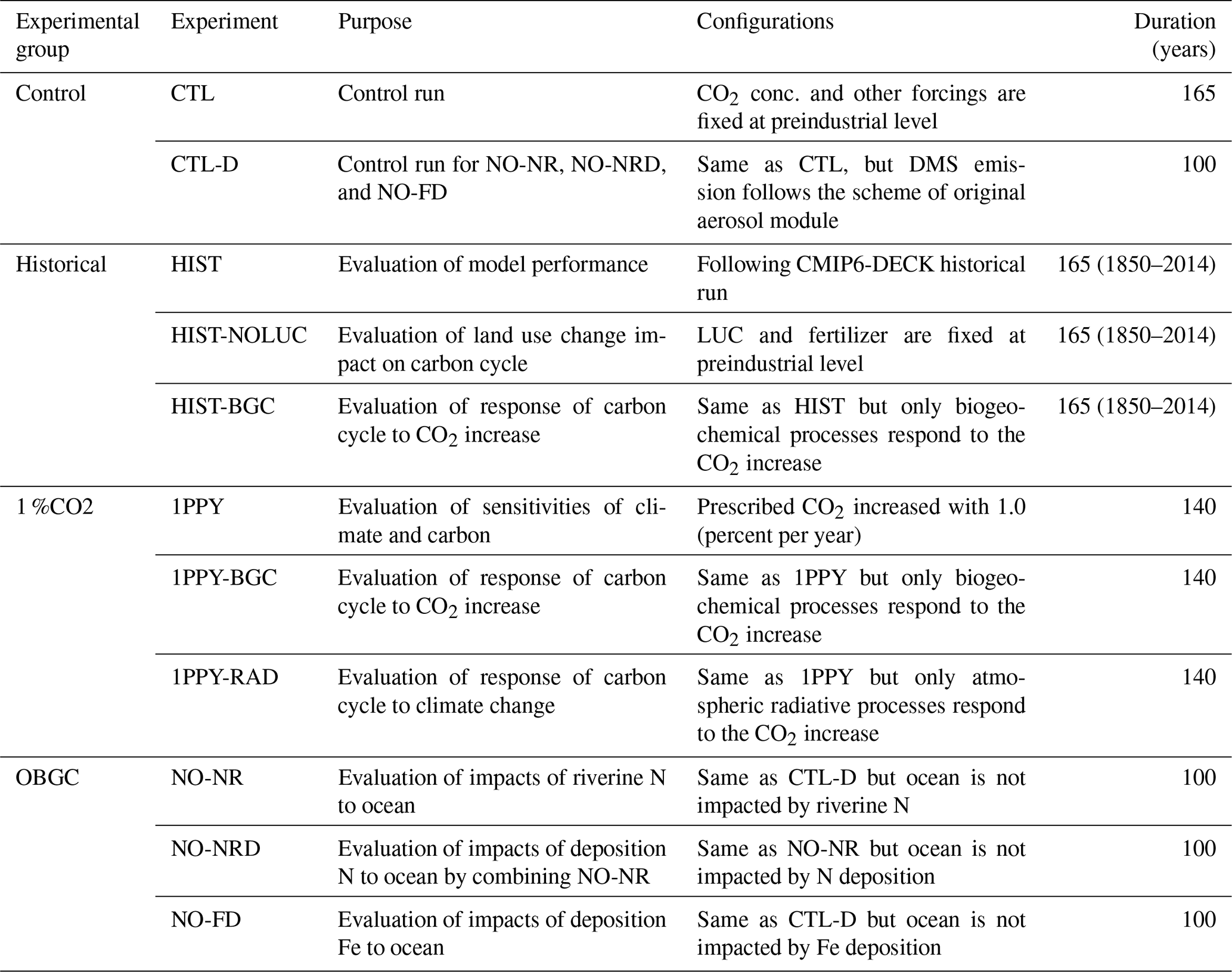
Table 2 Biogeochemical configurations in experiments, summarized as biogeochemical process settings. Bold characters represent the major differences between experiments within an experimental group.

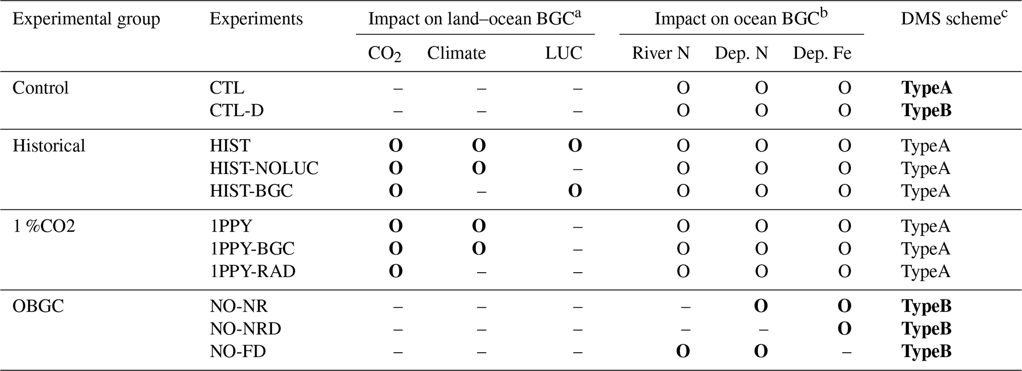
^a If the biogeochemical process in an experiment was affected by CO₂, climate, or land use change, the letter O is present; otherwise, the symbol – is used. ^b If the ocean biogeochemistry process detected fluxes of riverine nitrogen, atmospheric nitrogen deposition, or atmospheric iron deposition, the letter O is present; otherwise, the symbol – is used. ^c The TypeA DMS emission scheme is the default scheme in MIROC-ES2L, whereby DMS emissions are simulated as being dependent of the ocean biogeochemical states and the mixed-layer depth. TypeB is a scheme employed in the original aerosol component model in which DMS emissions are calculated independently of ocean biogeochemical states.

2.2.2 Evaluation of climate and carbon cycle response to CO₂

To evaluate the climate and carbon cycle response to CO₂ increase, we used the metrics of transient climate response (TCR), airborne fraction of CO₂ (AF), and TCRE, which have been previously used to characterize the entire climate–carbon cycle response to CO₂ increase in other models (Matthews et al., 2009; Hajima et al., 2012; Gillett et al., 2013). A similar analysis is made in this study, and the result is presented in Sect. 3.2.

First, TCRE is defined as the ratio of global mean near-surface air temperature change (T) to cumulative anthropogenic carbon emissions (CE) at the level of a doubled CO₂ concentration from the preindustrial state (hereafter, $\mathrm{2}\times {\mathrm{CO}}_{\mathrm{2}}^{\mathrm{PI}}$):

$$\begin{array}{}\text{(1)}& \mathrm{TCRE}=T/\mathrm{CE},\end{array}$$

which can be written as follows:

$$\begin{array}{}\text{(2)}& \mathrm{TCRE}=\left(\mathrm{CA}/\mathrm{CE}\right)\times (T/\mathrm{CA}),\end{array}$$

where CA is the atmospheric carbon increase until reaching $\mathrm{2}\times {\mathrm{CO}}_{\mathrm{2}}^{\mathrm{PI}}$. The first term on the right-hand side (CA∕CE) is identical to the definition of the cumulative airborne fraction of anthropogenic carbon emissions:

$$\begin{array}{}\text{(3)}& \mathrm{CA}/\mathrm{CE}=\mathrm{AF}.\end{array}$$

The second factor (T∕CA) can be represented by TCR as follows:

$$\begin{array}{}\text{(4)}& T/\mathrm{CA}=\mathrm{TCR}/\mathrm{CA},\end{array}$$

given that TCR is defined as T at $\mathrm{2}\times {\mathrm{CO}}_{\mathrm{2}}^{\mathrm{PI}}$. Thus, Eq. (2) can be expressed as follows:

$$\begin{array}{}\text{(5)}& \mathrm{TCRE}=\mathrm{AF}\times \left(\mathrm{TCR}/\mathrm{CA}\right).\end{array}$$

The result of the 1PPY simulation was used to evaluate TCRE, TCR, and AF. As CA is prescribed in the simulation, CE can be diagnosed by CE = CA + CL + CO, where CL and CO represent the change in land and ocean carbon storage, respectively. As shown by Matthews et al. (2009), AF summarizes the carbon cycle response to anthropogenic CE; the second term in Eq. (5) (TCR∕CA) captures the global temperature response to CO₂ increase in the models, and TCRE thus summarizes the two, i.e., the global temperature response to anthropogenic CO₂ emissions in the model.

To evaluate the strength of carbon cycle feedbacks in the model, the feedback strength is quantified by the so-called β and γ quantities (Friedlingstein et al., 2006; Arora et al., 2013). The former is a feedback parameter for CO₂–carbon feedback (carbon cycle response to atmospheric CO₂ increase), which can be calculated as follows:

$$\begin{array}{}\text{(6)}& {\displaystyle }& {\displaystyle }{\mathit{\beta }}_{\mathrm{L}}=\left({\mathrm{CL}}^{\mathrm{1}\mathrm{PPY}-\mathrm{BGC}}-{\mathrm{CL}}^{\mathrm{CTL}}\right)/{\mathrm{CA}}^{\mathrm{1}\mathrm{PPY}},\text{(7)}& {\displaystyle }& {\displaystyle }{\mathit{\beta }}_{\mathrm{O}}=\left({\mathrm{CO}}^{\mathrm{1}\mathrm{PPY}-\mathrm{BGC}}-{\mathrm{CO}}^{\mathrm{CTL}}\right)/{\mathrm{CA}}^{\mathrm{1}\mathrm{PPY}},\end{array}$$

where the subscripts L and O represent land and ocean, respectively, and the superscripts represent the experiment used for the calculation.

The quantity γ is a feedback parameter for climate–carbon feedback (carbon cycle response to climate change), which can be calculated using the results of the 1PPY-RAD and CTL simulations:

$$\begin{array}{}\text{(8)}& {\displaystyle }& {\displaystyle }{\mathit{\gamma }}_{\mathrm{L}}=\left({\mathrm{CL}}^{\mathrm{1}\mathrm{PPY}-\mathrm{RAD}}-{\mathrm{CL}}^{\mathrm{CTL}}\right)/T^{\mathrm{1}\mathrm{PPY}-\mathrm{RAD}},\text{(9)}& {\displaystyle }& {\displaystyle }{\mathit{\gamma }}_{\mathrm{O}}=\left({\mathrm{CO}}^{\mathrm{1}\mathrm{PPY}-\mathrm{RAD}}-{\mathrm{CO}}^{\mathrm{CTL}}\right)/T^{\mathrm{1}\mathrm{PPY}-\mathrm{RAD}}.\end{array}$$

3 Results and discussion

3.1 Model performance in historical simulation

3.1.1 Global climate: atmosphere and ocean physical fields

To evaluate the physical fields reproduced by MIROC-ES2L, the temporal evolutions of the global mean net radiation balance at the top of atmosphere (TOA) and anomalies of near-surface air temperature (SAT), sea surface temperature (SST), and upper-ocean (0–700 m) temperature were compared with observation datasets; the results are shown in Fig. 2. The model simulates a reasonably steady state of net TOA radiation balance in the CTL run, showing a trend of $-\mathrm{4.6}\times {\mathrm{10}}^{-\mathrm{5}}$ W m⁻² yr⁻¹ during the 165-year period. When comparing the net TOA radiation balance of the HIST simulation with satellite measurements (CERES EBAF-TOA edition 4.0 constrained by in situ measurements; Loeb et al., 2012, 2018), the model result is −0.63 W m⁻² (negative means net incoming radiation) during 2001–2010, which is within the range of $-\mathrm{0.5}\pm \mathrm{0.43}$ W m⁻² estimated by Loeb et al. (2012) for the corresponding period (Fig. 2a).

Following the net increase in incoming radiation, the SAT anomaly increases in the latter half of the 20th century (Fig. 2b). The warming trend during 1951–2011 is simulated as 0.1 K per decade, which is consistent with that of HadCRUT4 (version 4.6; Morice et al., 2012), i.e., 0.11 K per decade (Stocker et al., 2013). Observation datasets of SST (HadSST version 3.1.1; Kennedy et al., 2011) and upper-ocean temperature (Levitus et al., 2012) clearly display increasing trends in the corresponding period, which are successfully reproduced by the model (Fig. 2c and d). In addition to the warming trend in the latter half of the 20th century, the model captures the slowdown of SAT increase both in the 1950s and in the 1960s. These changes are likely induced by increased anthropogenic aerosol emissions and resultant cooling through indirect aerosol effects, together with cooling attributable to large volcanic eruptions in the 1960s (Wilcox et al., 2013; Nozawa et al., 2005). However, distinct deviations of the model results from HadCRUT4 are found for SAT and SST in the 1860s and particularly in the 1900s. This might be due to inevitable asynchronization between the simulation and observations on the phasing of the internal variability of the climate, as identified by Kosaka and Xie (2016). They reported that there should have been four major cooling events due to tropical Pacific variability in the 20th century, one of which was found in the 1900s. They also reported that the other three events were around 1940, 1970, and 2000; however, discrepancies arising from these three events are not so evident in this study, likely because of the single ensemble simulation. The model also exhibits a short-term response of the TOA radiation balance following episodic volcanic events (Fig. 2a, vertical dashed lines), with resultant cooling of SAT and SST (Fig. 2a–c) and further propagation into the deeper ocean with an extended cooling duration (Fig. 2d). Overall, the historical SAT increase in MIROC-ES2L, taking the difference between the averages of 1850–1900 and 2003–2012, is 0.69 K, while the HadCRUT4-based estimate by Stocker et al. (2013) is 0.78 K for the corresponding period. The model shows good performance in reproducing global physical fields. This is likely attributable to the inherited robust performance of the physical core of the model (MIROC5.2) because MIROC-ES2L has only two feedback pathways of biophysical processes on climate (DMS emissions from the ocean and terrestrial processes associated with LAI dynamics) when the model is driven by a prescribed CO₂ concentration. Both processes are likely to change the physical fields locally.

In addition to the radiation and temperature responses against historical external forcing, we briefly describe here the El Niño–Southern Oscillation (ENSO) and Atlantic meridional overturning circulation (AMOC) strength in MIROC-ES2L, both of which can affect interannual–multidecadal carbon cycle processes (Zickfeld et al., 2008; Pérez et al., 2013; Friedlingstein, 2015). In the HIST experiment, the standard deviation of the monthly SST anomaly in the Niño-3 region (5^∘ S–5^∘ N, 90–150^∘ W) was 1.57 K in 1950–2009, which is larger than that of HadSST (0.94 K). This unrealistically large ENSO amplitude tends to influence the simulated interannual global temperature variability (Fig. 2b), which is suggestive of a further effect on the interannual variability in biogeochemical fields (e.g., CO₂ flux in the tropics). The AMOC intensity, quantified by North Atlantic Deep Water transport across 26.5^∘ N, was approximately 13 Sv (1 Sv =10⁶ m³ s⁻¹) as the 1850–2014 average, which is smaller than the observational estimates of 17.2 Sv (McCarthy et al., 2015). In the HIST run, the AMOC strength was weakened at a rate of 0.01 Sv yr⁻¹ (i.e., reduction of 1.7 Sv during the 165 years of HIST), which seems slightly smaller than the recent estimate of AMOC weakening of 3±1 Sv from the mid-20th century (Caesar et al., 2018).

Figure 2 Comparison of HIST simulation results by MIROC-ES2L with observations: anomalies of (a) net radiation balance at the top of the atmosphere (TOA; upward positive), (b) global mean surface air temperature, (c) global mean sea surface temperature, and (d) global mean ocean temperature at 0–700 m of depth. Black, red, and blue lines represent historical simulations, historical observations, and pi-control simulations, respectively. Vertical dashed lines represent the timing of major volcanic eruptions (i.e., Krakatau in 1883, Santa Maria in 1902, Agung in 1963, El Chichón in 1982, and Pinatubo in 1991). In panel (a), the simulation results are presented as anomalies from the 1850–2014 average of the CTL run. In panels (b), (c), and (d), the results are presented as the anomalies from the 1961–1990 averages. Observation data for the radiation balance were obtained from the global product of CERES EBAF-TOA edition 4.0. Observation data for SAT and SST were obtained from HadCRUT4 (Morice et al., 2012) version 4.6 and HadSST (Kennedy et al., 2011) version 3.1.1, respectively. The ocean temperature anomaly updated from Levitus et al. (2012) is used to compare ocean temperature at 0–700 m of depth during the period 1955–2014.

Hereafter, we present an overview of the performance of the mean state of the physical fields, atmosphere, and land–ocean basic variables of the model in comparison with various observational-based data. The variables examined here are SAT, precipitation, SST, sea ice concentration, land snow cover, and mixed-layer depth, all of which are representative physical states associated with biogeochemical processes. The mixed-layer depth is defined as the depth at which the potential density becomes larger than that of the sea surface by 0.125 kg m⁻³. Figure 3 shows the climatology of SAT (air temperature at 2 m of height) averaged over 1989–2009 for annual, December–February (DJF), and June–August (JJA) means and the biases in comparison with the ERA-Interim dataset (Dee et al., 2011). The comparison suggests that the model performs well (biases <2 ^∘C) over the tropics and most of the global area in terms of both annual mean and seasonality. However, obvious warm biases exist over the Southern Ocean and Antarctica. This is a general tendency of CMIP5-class models, and both MIROC5 (Watanabe et al., 2010) and MIROC6 (Tatebe et al., 2019) also suffer from this problem. The warm bias in the Southern Ocean can be mainly attributed to a poor representation of cloud radiative processes (Bodas-Salcedo et al., 2012; Williams et al., 2013; Hyder et al., 2018) but also poor representations of the mixed-layer depth and deep convection in the open ocean attributable to the lack of modeled mesoscale processes in the Antarctic Circumpolar Current (Tatebe et al., 2019). A related warm bias in SST over the Southern Ocean is also confirmed, which is discussed later.

Figure 4 shows the precipitation distribution in the HIST experiment in comparison with the Global Precipitation Climatology Project (GPCP) dataset (Adler et al., 2003). Generally, the precipitation distribution is reasonably well represented in the model. The Intertropical Convergence Zone is reproduced well in the experiment, except that the simulated South Pacific Convergence Zone is shifted equatorward relative to the GPCP, which is the so-called double Intertropical Convergence Zone syndrome (Bellucci et al., 2010). Over continental areas, the model is effective in capturing the spatial pattern of both the annual mean precipitation and the seasonality. However, positive precipitation biases are evident in some tropical land regions such as central Africa, South and Southeast Asia, and South America. Additionally, arid and semiarid regions of central Asia, Australia, and the western side of North America also show a positive precipitation bias, although it is unclear in the bias map (see Supplement Fig. S6 for a comparison with the absolute precipitation rate of GPCP).

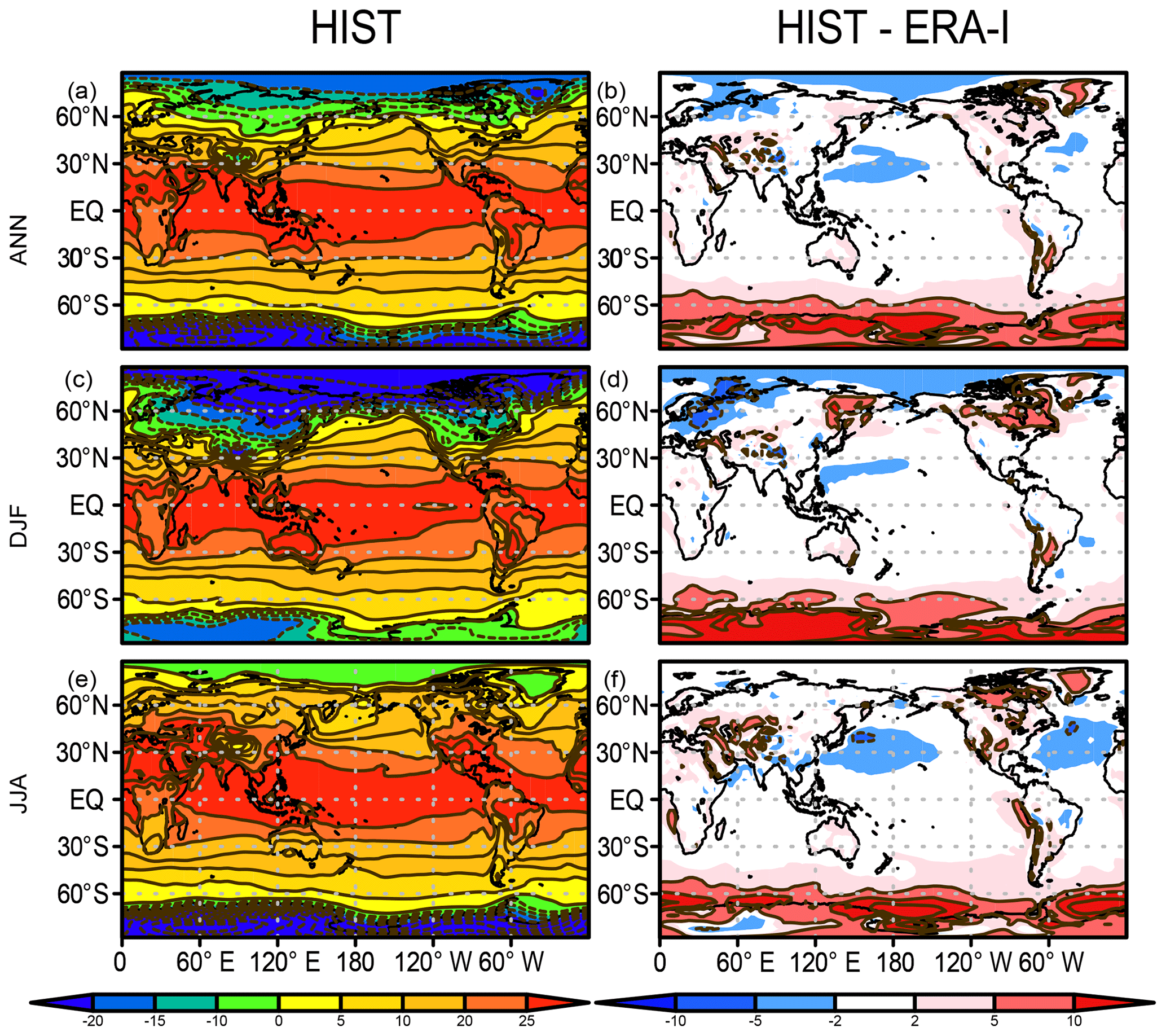
Figure 3 Air temperature at 2 m of height (^∘C) in the HIST simulation presented as a 1989–2009 climatology and the bias compared with the ERA-Interim dataset (Dee et al., 2011) for (a, b) annual, (c, d) DJF, and (e, f) JJA means.

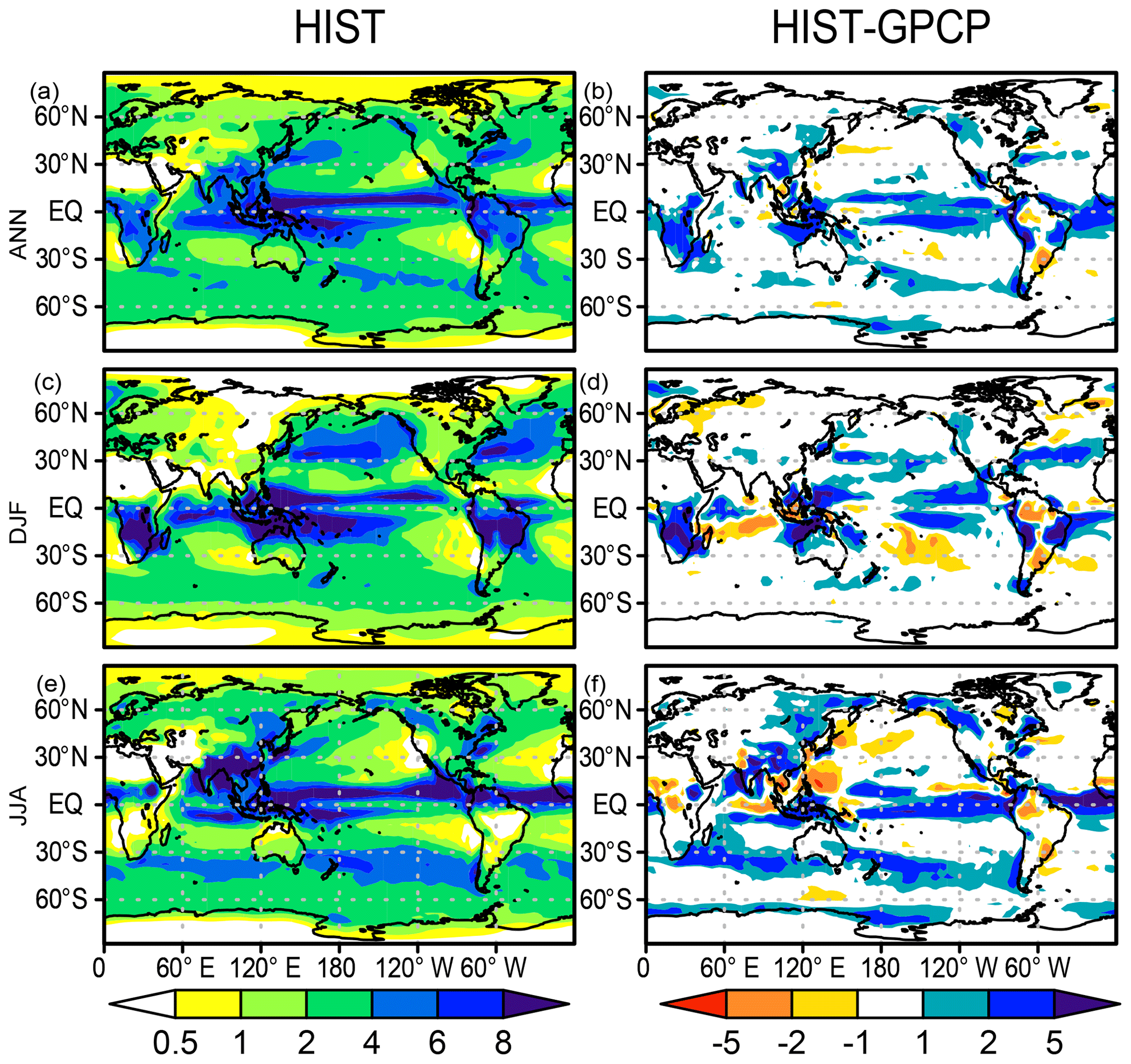
Figure 4 Precipitation distributions (mm d⁻¹) in the HIST simulation and biases relative to the GPCP dataset (Adler et al., 2003) for (a, b) annual, (c, d) DJF, and (e, f) JJA means averaged over 1981–2000.

When projecting future climate change, it is important for a model to reproduce the observed climatological patterns of key physical variables, as suggested by Ohgaito and Abe-Ouchi (2009). The biogeochemical tracers are also affected by the representation of the physical fields. Figure 5 presents the modeled SST and its bias with respect to the World Ocean Atlas 2013 (Locarnini et al., 2013). Generally, the model performs well, confirmed by the large extent of the area with minimal bias (colored white in Fig. 5). However, obvious bias is evident, e.g., the warm bias in the Southern Ocean, as already explained above (Fig. 3). A cold bias is also evident over the western North Pacific Ocean, which is attributable to the lack of narrow and swift western boundary currents owing to the coarse horizontal resolution in the ocean parts of the present ESM.

The model performance in simulating sea ice concentration and snow cover over land for both March and September is shown in Fig. 6 in comparison with observational data (Special Sensor Microwave Imager (SSM/I; Kaleschke et al., 2001) for sea ice concentration and the Moderate-resolution Imaging Spectroradiometer (MODIS; Hall et al., 2006) for snow cover. Sea ice extent in the Northern Hemisphere is represented well for both months, although the summertime concentration minimum is slightly smaller than observed. In the Southern Hemisphere, however, the sea ice extent is unrealistically underestimated because of the persistent warm bias described above. The extent of the snow-covered area is also represented well, likely owing to the updated scheme for subgrid snow representation (Nitta et al., 2014; Tatebe et al., 2019). However, the fine structure of the snow cover is lost in the simulation, which is likely attributable to the coarse resolution of the modeled atmosphere and land. The reasonable performance in reproducing land snow seasonality in the boreal region is important for land biogeochemistry and the physical climate because snowmelt (accumulation) and leaf flush (shedding) processes are mutually associated (Supplement Fig. S7).

Figure 7 shows the mixed-layer depth in comparison with the mixed-layer dataset of Argo with grid point value (MILA_GPV; Hosoda et al., 2010). The HIST simulation captures both the spatial pattern and the seasonality change in mixed-layer depth. In the Northern Hemisphere winter, the structure of the deep mixed layer over the western North Pacific is consistent with observations; however, the actual depth is overestimated owing to the lack of mesoscale eddies. The deep mixed layer in the subarctic North Atlantic is also consistent with observations, except there is less deep water formed in the Labrador Sea. Additionally, the shallow mixed layer in low latitudes is generally captured well by the simulation, and the depth that is maintained at around 100 m over the Southern Ocean is consistent with observations. In austral winter, MILA_GPV shows that the mixed layer develops to more than 200 m over the Indian Ocean and the Pacific sector of the Southern Ocean, whereas it is shallow (around 50 m) in the tropics and the Northern Hemisphere (Fig. 7d). The model captures the general pattern in austral winter, although the extent of the simulated deeper mixed-layer depth of more than 200 m in the Southern Ocean is larger than that of MILA_GPV (Fig. 7c).

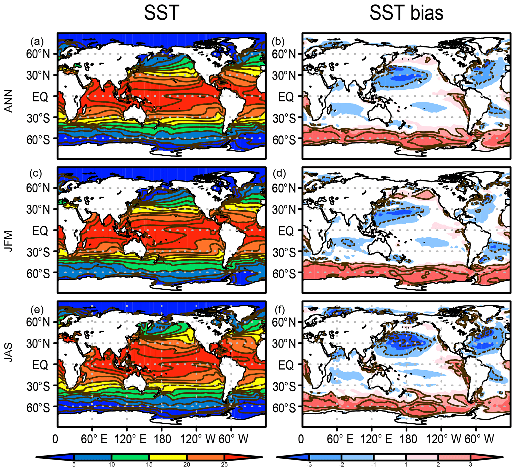
Figure 5 SST (^∘C) in the HIST simulation presented as a 1955–2012 climatology and the bias in comparison with WOA2013 (Locarnini et al., 2013) for (a, b) annual, (c, d) JFM, and (e, f) JAS means.

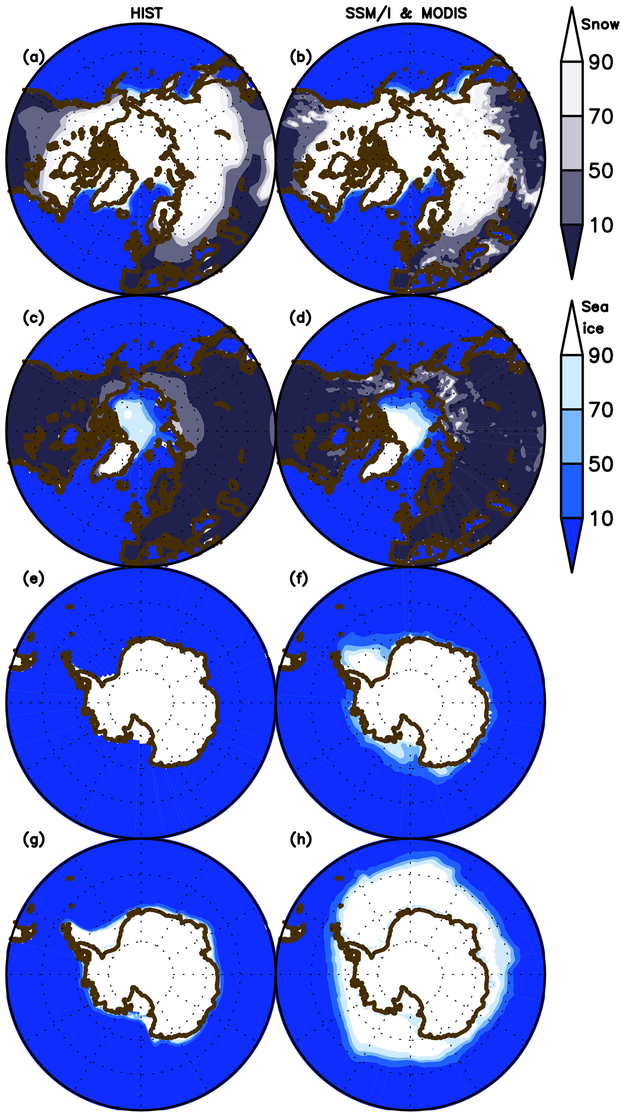
Figure 6 Northern Hemisphere sea ice concentration and land snow fraction (%) in the HIST simulation presented as a 2003–2013 climatology and in comparison with SSM/I (Kaleschke et al., 2001) and MODIS (Hall et al., 2006) data for (a, b) March and (c, d) September.

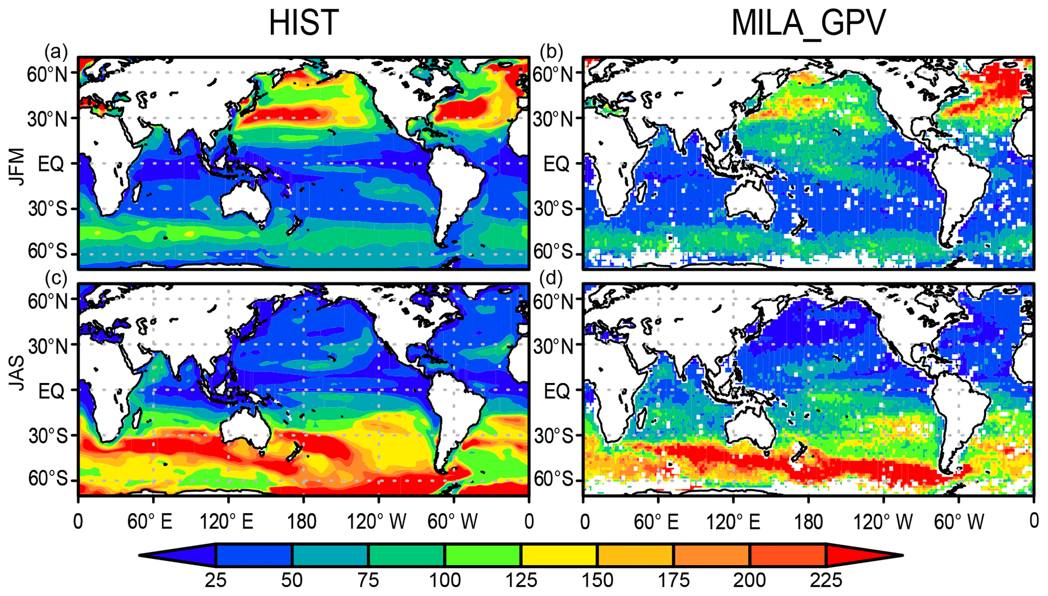
Figure 7 Mixed-layer depth (m) in the HIST simulation presented as a 2000–2010 climatology and comparison with the MILA_GPV dataset (Hosoda et al., 2010) for (a, b) JFM and (c, d) JAS means.

3.1.2 Global carbon budget

The simulated net CO₂ uptake by land and ocean in cumulative values (i.e., changes in total carbon of land and ocean) is shown in Fig. 8a and b, respectively. For land, the CTL run shows a slight reduction of carbon of 7.6 PgC during the 165 years (i.e., 4.6 PgC per century), which is within the acceptable range for the CMIP6 exercise (10 PgC per century; Jones et al., 2016). The dashed gray line in Fig. 8a is the result from HIST-NOLUC and shows a natural land carbon sink in MIROC-ES2L of 200 PgC during 1850–2014. This is comparable with the estimate of 185±50 PgC by Le Quéré et al. (2018) for the same period (vertical gray bar in Fig. 8a), which was obtained from multiple offline terrestrial ecosystem models with fixed land use. Additionally, LUC is one of the factors that drastically changes the historical land carbon amount because positive (negative) LUC emissions are directly linked to a reduction (increase) in land carbon. Based on bookkeeping methods, Le Quéré et al. (2018) estimated the cumulative CE derived from LUC during 1850–2014 as 195±75 PgC, whereas the simulated cumulative emissions by MIROC-ES2L diagnosed by the difference in land carbon amount between HIST-NOLUC and HIST are 156 PgC.

Through being affected by both environmental changes and LUCs, MIROC-ES2L demonstrates in the HIST simulation that land carbon is reduced by approximately 60 PgC from the beginning of the simulation until the middle of the 20th century (black line in Fig. 8a). This reduction should reflect LUC during this period because HIST-NOLUC does not show such a trend of decrease in the corresponding period (dashed gray line in Fig. 8a). From the 1960s, the model shows continuous carbon sequestration on land, which results in a positive net CO₂ uptake of 2.4 PgC yr⁻¹ in the 2000s (Table 3). This continuous increase in the latter half of the 20th century is due to the combined effects of CO₂ fertilization, vegetation recovery associated with LUC, and the increase in nitrogen input via deposition and the use of fertilizer. This is clearly displayed in Fig. 8c, where the historical land carbon change is decomposed into the responses to (1) CO₂ increase (blue line, diagnosed by HIST-NOLUC + HIST-BGC – HIST; see Table 2), (2) climate change (red line, by HIST – HIST-BGC), and (3) LUC (green line, by HIST – HIST-NOLUC). In the latter half of the 20th century, land carbon sequestration accelerated by CO₂ stimulation is clear, while climate change and the resultant terrestrial carbon loss also become evident. Additionally, land carbon reduction induced by LUC is slightly weakened in the corresponding period. During the historical period, MIROC-ES2L simulates a total land carbon change (CL) of 44 PgC. This number drops to within the independent estimate range of $-\mathrm{10}\pm \mathrm{90}$ PgC (vertical black bar in Fig. 8a), and the estimation uncertainties take into account both the terrestrial natural carbon sink and LUC emissions (calculated as (${\mathit{\sigma }}_{\mathrm{LUC}}^{\mathrm{2}}+{\mathit{\sigma }}_{\mathrm{SINK}}^{\mathrm{2}}{)}^{\mathrm{0.5}}$, where σ_LUC and σ_SINK represent the uncertainty range of LUC emissions and the land sink, respectively, in Le Quéré et al., 2018). The possible range for CL can be changed if we estimate it as the residual of other global carbon budgets (i.e., CL = FF – CA – CO, where FF is the cumulative fossil fuel carbon emission). Using the estimated ranges of FF, CA, and CO reported by Le Quéré et al. (2018) (i.e., 400±20, 235±5, and 150±20 PgC, respectively; the budget imbalance of 25 PgC is ignored here), the CL range is suggested to be 15±29 PgC. In this case, the result of MIROC-ES2L (44 PgC) is still within the estimation boundaries, although it is at the upper end of the suggested range.

For the ocean, the model shows an increase in carbon accumulation in the CTL run (Fig. 8b). This is partly because of carbon removal by the sedimentation process that is newly introduced into MIROC-ES2L. In this process, an amount of carbon is extracted from the ocean bottom, which should be compensated for by an equivalent input of carbon from the atmosphere through gas exchange processes. In the CTL run, the rate of carbon extracted from the ocean bottom is 0.068 PgC yr⁻¹ (Table 4), which suggests that the process removes 11 PgC throughout the entire simulation period of CTL (165 years). It is noted that Ciais et al. (2013) suggested that the ocean was a net source of CO₂ in the preindustrial era to an amount of 0.7 PgC yr⁻¹, whereas our model shows it as a net sink in the same condition. This is likely attributable to the lack of a process of riverine carbon input in our model. For example, Ciais et al. (2013) estimated that the ocean obtains an external carbon input of 0.9 PgC yr⁻¹ from rivers, 0.2 PgC yr⁻¹ of which is removed by ocean sedimentation and 0.7 PgC yr⁻¹ is lost from the ocean to the atmosphere via gaseous exchange. The sedimentation process cannot explain all the increase in oceanic carbon in the CTL run (30 PgC). Therefore, the remainder should be attributed to other reasons, e.g., the shortness of the spin-up period or imperfect mass conservation in the ocean biogeochemical component.

The HIST run shows the cumulative carbon uptake by the ocean, which is predominantly driven by CO₂ increase (Fig. 8b and d). In comparison with land, ocean carbon shows a relatively small response to climate change (red line in Fig. 8d), which is consistent with analysis of the carbon cycle feedback in an idealized scenario (Arora et al., 2013). Furthermore, the model shows weak or almost no response against LUC (green line in Fig. 8d), although the ocean component in the model actually receives increased nitrogen input from rivers attributable to LUC and agriculture (Fig. 9, Table 4). This suggests that the increase in riverine nitrogen input due to LUC and agriculture would not induce a significant global-scale impact on ocean carbon uptake in the historical period. The model simulates a cumulative carbon uptake of 163 PgC for 1850–2014, which is within the range of 150±20 PgC (vertical black bar in Fig. 8b) reported by Le Quéré et al. (2018).

Overall, MIROC-ES2L qualitatively captures the temporal evolution of carbon dynamics in the historical period; the cumulative carbon uptake by both land and ocean is within the range of the estimates by Le Quéré et al. (2018). However, the model might overestimate the net carbon uptake by the land and/or ocean or underestimate LUC emissions. This is because the cumulative fossil fuel emissions, diagnosed from the simulated atmosphere–land–ocean CO₂ fluxes and prescribed CO₂ concentration change (FF = CA + CL + CO; Appendix D), were 447 PgC, i.e., larger than the estimate of 400±20 PgC of Le Quéré et al. (2018). Additionally, this speculation is also supported by the diagnosed CO₂ concentration at the end of the HIST run (Appendix D); the diagnosed concentration is 376 ppmv, which is lower (by 22 ppmv) than that actually monitored. We note, however, that the likely biases in land–ocean carbon uptake, suggested by the larger diagnosed emissions and lower diagnosed CO₂ concentration, could be partially alleviated if the model were driven by anthropogenic CO₂ emissions. This is because in emission-driven mode, the relatively stronger land–ocean carbon uptake leads to a lower atmospheric CO₂ concentration, which could weaken the land and ocean sink through a negative CO₂–carbon feedback. Indeed, in emission-driven mode, the atmospheric CO₂ concentration in the historical run (esm-historical; Jones et al., 2016) is simulated to be 384 ppmv in 2014 (as an average of three ensemble experiments; data not shown but available via the Earth System Grid Federation servers), which is closer to the actual level monitored (but still lower by 14 ppmv). Additionally, in emission-driven mode, the land and ocean are mutually interlinked via the atmospheric CO₂ concentration; thus, a strong bias of CO₂ flux in one component can be modulated by the other. This mechanism might reduce the bias of CO₂ fluxes of the land and ocean simultaneously, or it might exacerbate the CO₂ flux by imposing the flux bias of one onto the other. For more detail, simulations and multimodel analyses based on emission-driven configurations are necessary, as designed in C4MIP (Jones et al., 2016).

Figure 8 Land and ocean carbon change (i.e., cumulative net carbon uptake by land and ocean) in historical simulations. (a, b) Simulation results of the historical (HIST, black lines), historical without land use change (HIST-NOLUC, dashed gray), historical without climate change (HIST-BGC, dashed red), and control (CTL, dashed blue) runs. For land calculation, the carbon amount change in product pools for land use is considered. Vertical bars represent uncertainty ranges estimated from Le Quéré et al. (2018). Black bars correspond to the HIST (1850–2014) run result, and the gray bar represents the uncertainty range for the natural carbon sink of land, which corresponds to the HIST-NOLUC run in this study. (c, d) The HIST run result shown again (black lines) together with the decomposed response of land–ocean carbon driven only by CO₂ increase (dashed blue), climate change (dashed red), and LUC (dashed green). Note that the ocean in MIROC-ES2L considers carbon removal via the sedimentation process onto ocean floor; thus, the model exhibits continuous carbon uptake, even in the CTL experiment.

Table 3 Key variables of global land biogeochemistry: preindustrial condition (average of 10 years) and the 2000s in the historical run (HIST).

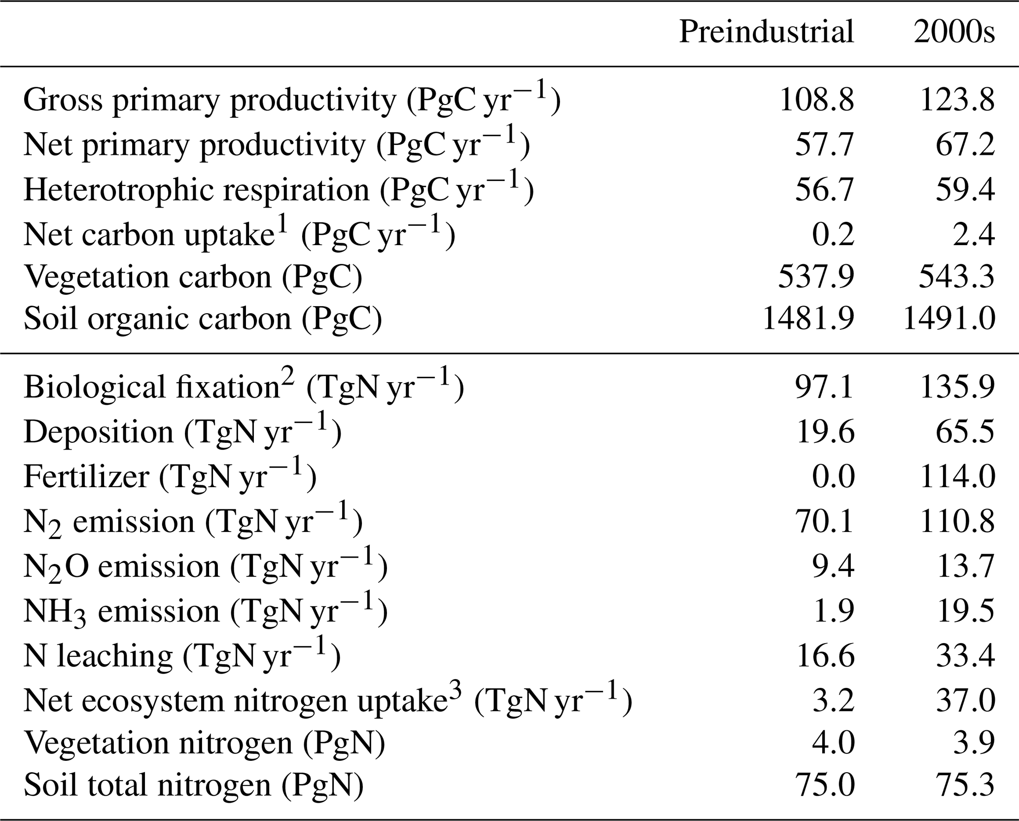
¹ Net carbon uptake is calculated as the net ecosystem productivity minus the carbon emissions from product pools for land use. ² BNF by agriculture is also included. ³ Net nitrogen uptake is calculated by annual changes in total nitrogen storage.

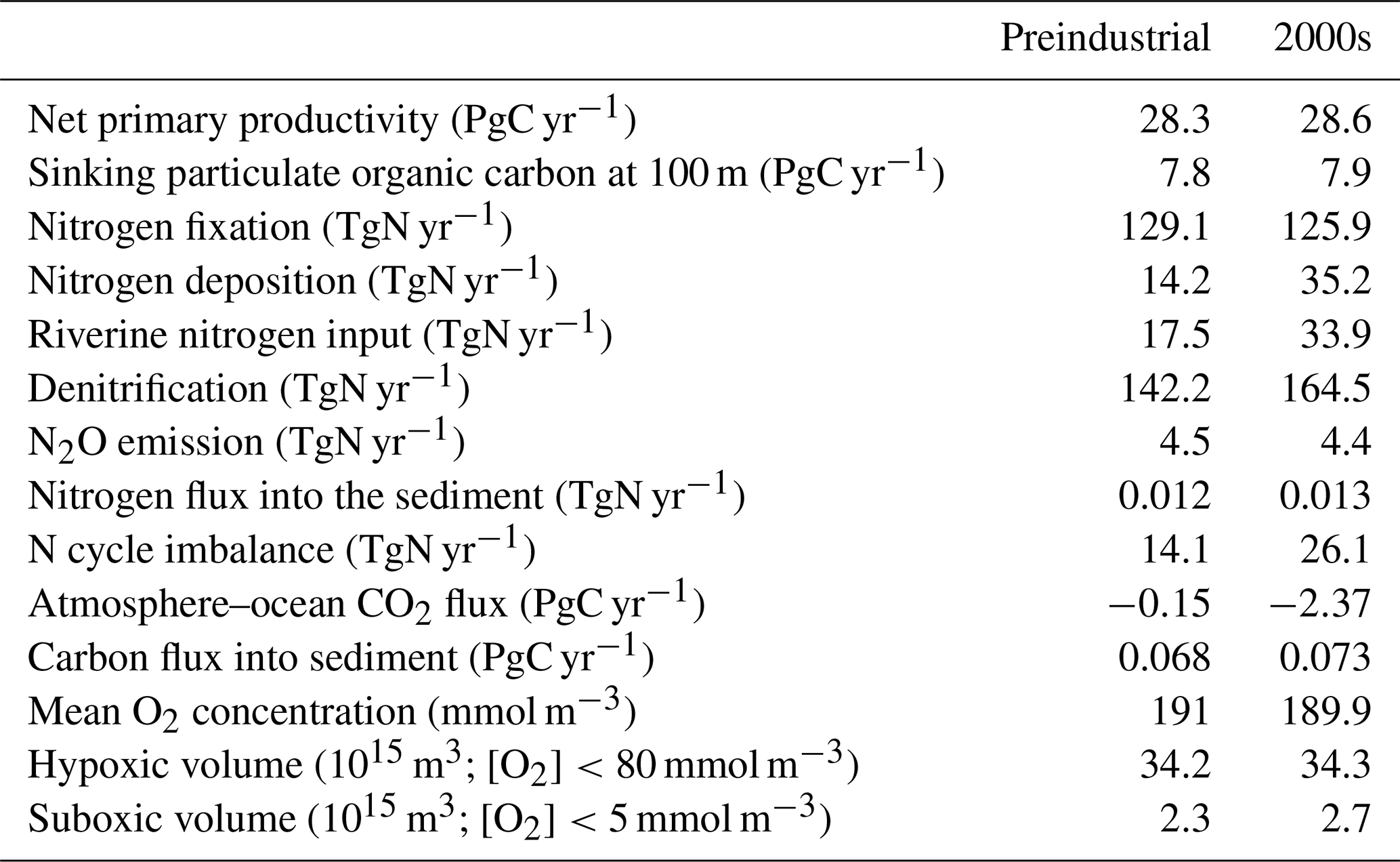
Table 4 Key global ocean biogeochemical fluxes and concentrations under the preindustrial control simulation and the 2000s.

3.1.3 Global nitrogen budget

MIROC-ES2L can simulate the global nitrogen cycle under interaction with the climate and carbon cycle, and the global N budget for land and ocean in the HIST simulation is shown in Fig. 9 as the component fluxes. Comparison of the terrestrial nitrogen budget in the 2000s with the preindustrial condition (Table 3) reveals that the annual inputs of nitrogen via deposition and fertilizer, which are controlled by forcing data, increase to 65.5 and 114 TgN yr⁻¹, respectively. Additionally, BNF is also increased by 40 % (39 TgN yr⁻¹), which is caused by the areal expansion of agriculture for N-fixing crops (Fig. 9, Supplement Fig. S8). Previous studies have shown similar levels of increase. For example, Gruber and Galloway (2008) reported a value of 35 TgN yr⁻¹, and the absolute magnitude of agricultural BNF in the present-day condition was estimated as 50–70 TgN yr⁻¹ by Herridge et al. (2008) and 40 TgN yr⁻¹ by Galloway et al. (2008).

For terrestrial nitrogen efflux, Gruber and Galloway (2008) reported N₂ emissions in the unperturbed state as 100 TgN yr⁻¹, i.e., larger than found in this study (72 TgN yr⁻¹). However, in the present-day condition, they estimated the absolute magnitude of N₂ emissions as 115 TgN yr⁻¹, which is reasonably close to our model result (111 TgN yr⁻¹). MIROC-ES2L simulates the historical increase in N₂O emission from soil as 4.3 TgN yr⁻¹ from the preindustrial condition to the 2000s, which is comparable with the estimate of approximately 4 TgN yr⁻¹ for 1861–2015 derived from a model comparison study (Tian et al., 2018). However, the absolute magnitude of terrestrial N₂O emission fluxes in preindustrial and present-day conditions is likely overestimated (Table 3; Hashimoto, 2012).

Although it is difficult to obtain observation-based estimates of how much nitrogen was accumulated by the land ecosystem in the historical period, the model demonstrates net nitrogen uptake by land in the 2000s as 37 TgN yr⁻¹ (Table 3). This positive uptake is likely caused by increased total nitrogen input into the land ecosystem. In addition to the increasing N input, the net positive N uptake by land is likely accelerated by the increased nitrogen demand by plants and soils that have higher C:N ratios under elevated CO₂ concentrations. This is because the net increase in land N uptake is also found in 1PPY-BGC (Supplement Table S1), even though the N inputs such as BNF, fertilizer, deposition, and climate conditions in the 1PPY-BGC simulation are almost unchanged from the CTL run. This suggests that atmospheric CO₂ increase in HIST has changed the C:N ratios in plants and soil and hence stimulated ecosystem nitrogen demand. The model demonstrates nitrogen loss by LUC at a rate of >50 TgN yr⁻¹ (Fig. 9). This is because the harvested biomass in the model is translocated to product pools, and the nitrogen contained in the biomass is assumed lost with implicit chemical form, together with carbon loss as CO₂.

Compared with land, the model simulates relatively stable dynamics of the oceanic nitrogen budget but with larger interannual variation (Fig. 9b). In the 2000s, oceanic BNF is simulated as 126 TgN yr⁻¹, which is almost at the same level (slightly below) as that of the preindustrial state, i.e., 129 TgN yr⁻¹ (Table 4). This number is close to previously reported estimates of approximately 130 TgN yr⁻¹ (Eugster and Gruber, 2012). The invariant behavior of BNF in the model suggests that the historical change in nitrogen input into the ocean is primarily attributable to two external sources: deposition and riverine input. Nitrogen deposition into the ocean, which is prescribed in the forcing data, shows an increase from 14 TgN yr⁻¹ in the preindustrial condition to 35 TgN yr⁻¹ in the 2000s. Riverine nitrogen input at a river mouth is shown to increase from 17.5 TgN yr⁻¹ in the preindustrial condition to 33.9 TgN yr⁻¹ in the 2000s (Table 4; this is discussed further in Sect. 3.1.5 and 3.2.3). In this study, the gross nitrogen input into the ocean in the present-day condition is simulated as 195 TgN yr⁻¹. The value is reasonably close to the estimate of 200 TgN yr⁻¹ by Wang et al. (2019) and that of 209 TgN yr⁻¹ by Galloway et al. (2004); however, it is smaller than other published estimates (e.g., 294 TgN yr⁻¹, Codispoti et al., 2001; 270 TgN yr⁻¹, Gruber and Galloway, 2008). Denitrification, the main source of ocean nitrogen loss, is simulated as 142 TgN yr⁻¹ for the preindustrial condition and 165 TgN yr⁻¹ for the 2000s. These values are within the wide range of total denitrification rates estimated by previous studies, i.e., 145–450 TgN yr⁻¹ (Eugster and Gruber, 2012). It should be noted that the present model used in this study does not include sedimentary denitrification. Thus, the expected N flux by sedimentary denitrification is imposed on water-column denitrification, and the rate of water-column denitrification is likely overestimated. Overall, the model exhibits an oceanic N imbalance of 26.1 TgN yr⁻¹ in the present-day condition (Fig. 9, Table 4).

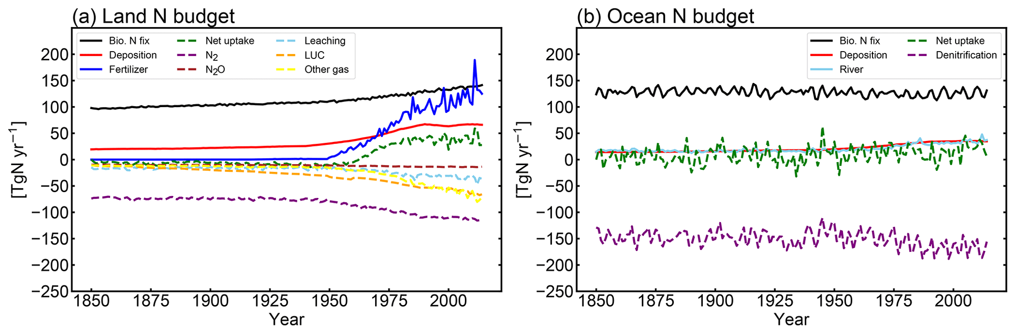
Figure 9 Rate of change of the global nitrogen budget in the (a) land and (b) ocean in the HIST simulation. Solid lines represent the nitrogen input into the land and ocean, and dashed lines represent its fate. Positive (negative) values mean a flux into (out of) the land and ocean. In panel (a), BNF (black line) considers both natural and agricultural fluxes. LUC (dashed orange line) is an emission derived from the decay of biomass in the LUC product pools. Other gases (yellow line) represent the sum of NH₃ emissions and the flux from abiotic sources. For the ocean, denitrification (purple line) includes both N₂ and N₂O emissions. The rate of nitrogen loss by the sedimentation process onto the ocean floor is not shown in the figure because of the small size of the flux (<0.015 TgN yr⁻¹). All nitrogen gas emissions are diagnosed and thus have no effect on the radiative balance in the atmosphere or on air quality change.

3.1.4 Land biogeochemistry

Model performance in relation to land biogeochemistry is evaluated based on the spatial distributions of three fundamental variables of the land carbon cycle in comparison with observation-based products. First, GPP in the HIST simulation is compared with the global product by Jung et al. (2011) (Fig. 10a–c). The model simulates high productivity (>2000 gC m⁻²) in the tropical forests of central Africa, Southeast Asia, and South America, although the productivity in these regions is generally still underestimated in comparison with the observation-based product. This underestimation is likely attributable to the use of the parameter values of photosynthetic capacities (K_PSAT1 and K_PSAT2 in Appendix A) from Kattge et al. (2009). This is because Kattge et al. (2009) also showed substantial depression of photosynthetic capacity in the tropics. The model captures the moderate productivity of vegetation in savanna regions such as the eastern side of South America and the marginal region surrounding central Africa. Moderate GPP is also found in the Northern Hemisphere in the region 20–45^∘ N, where a large proportion of land cover is dominated by both natural and agricultural vegetation (Supplement Fig. S2). The GPP gradient from moderate to lower GPP in the boreal to tundra regions of Eurasia and North America is captured well by the model. The model estimates global GPP at 124 PgC yr⁻¹ in the 2000s (Table 3), which is within the range of 106–140 PgC yr⁻¹ produced by the CMIP5 ESMs and is reasonably close to the value of 119 PgC yr⁻¹ derived from an observation product (1986–2005 average; Jung et al., 2011). The simulated GPP seasonality is also compared with that of Jung et al. (2011) (Supplement Fig. S9). It reveals a reasonable summertime peak and the seasonality of GPP in the extratropical Northern–Southern Hemisphere, where vegetation phenology is primarily controlled by air temperature. However, the region around 40^∘ N displays a longer growing season than that of Jung et al. (2011), and the tropics (20^∘ S–20^∘ N) show less seasonality, suggesting room for improvement of the phenology-related processes and surface climate fields in the corresponding region or biome types.

To evaluate the simulated vegetation carbon, we compare the model results of forest carbon, not total vegetation carbon, with those of Kindermann et al. (2008) (Fig. 10d–f). The model reproduces the reasonably high density of biomass in tropical forests, although the values are smaller than the observation product (Fig. 10f). This is partly attributable to the underestimation of GPP in this region, as described above. In high-latitude regions of the Northern Hemisphere (around 50^∘ N), the model overestimates biomass density, particularly in terms of the evergreen coniferous forests that extend across western Siberia and North America. GPP in these regions is captured reasonably well by the model (Fig. 10a and b), and thus the overestimation of boreal forest biomass is likely due to the underestimated turnover rate of forest carbon. A slight overestimation of biomass is also found in regions where intensive cultivation has occurred, i.e., Europe, Southeast–East Asia, and eastern America. The model estimates global vegetation carbon content including all types of vegetation at 543 PgC (Table 3).

In Fig. 10g–i, the model results of soil organic carbon (SOC) are compared with two different types of SOC products: harmonized soil property values for broad-scale modeling (WISE30sec) by Batjes (2016) and the Northern Circumpolar Soil Carbon Database version 2 (NCSCDv2) by Hugelius et al. (2013). The former is a global dataset that represents soil column SOC down to the depth of 2 m, whereas the latter targets only the high-latitudinal region of the Northern Hemisphere at different soil depths (∼1, ∼2, and ∼3 m). Comparison with WISE30sec confirms that the model successfully captures the spatial distribution of lower carbon accumulation in arid and tropical regions and higher SOC in boreal regions in the Northern Hemisphere. However, the simulated zonal mean SOC in the boreal regions is about half that of WISE30sec (Fig. 10i). This is likely attributable to the different treatment of frozen carbon in deeper soils in permafrost regions; i.e., WISE30sec covers the total SOC down to 2 m of depth including frozen carbon, while the model does not consider the frozen carbon and instead simulates only upper SOC as litter and lower SOC as humus. The model result in the boreal region is comparable with the NCSCDv2 estimation for 1 m of depth. We note, as mentioned by Todd-Brown et al. (2012), that large uncertainty remains in the estimation of the SOC amount, especially in boreal regions. Globally, SOC is simulated as 1491 PgC (Table 3) in this study, which is smaller than the value of 2060±215 PgC of WISE30sec (Batjes, 2016) but comparable with the range of 890–1660 PgC, as estimated by Todd-Brown et al. (2012) based on the Harmonized World Soil Database v1.2 (FAO/IIASA/ISRIC/ISS-CAS/JRC, 2012).

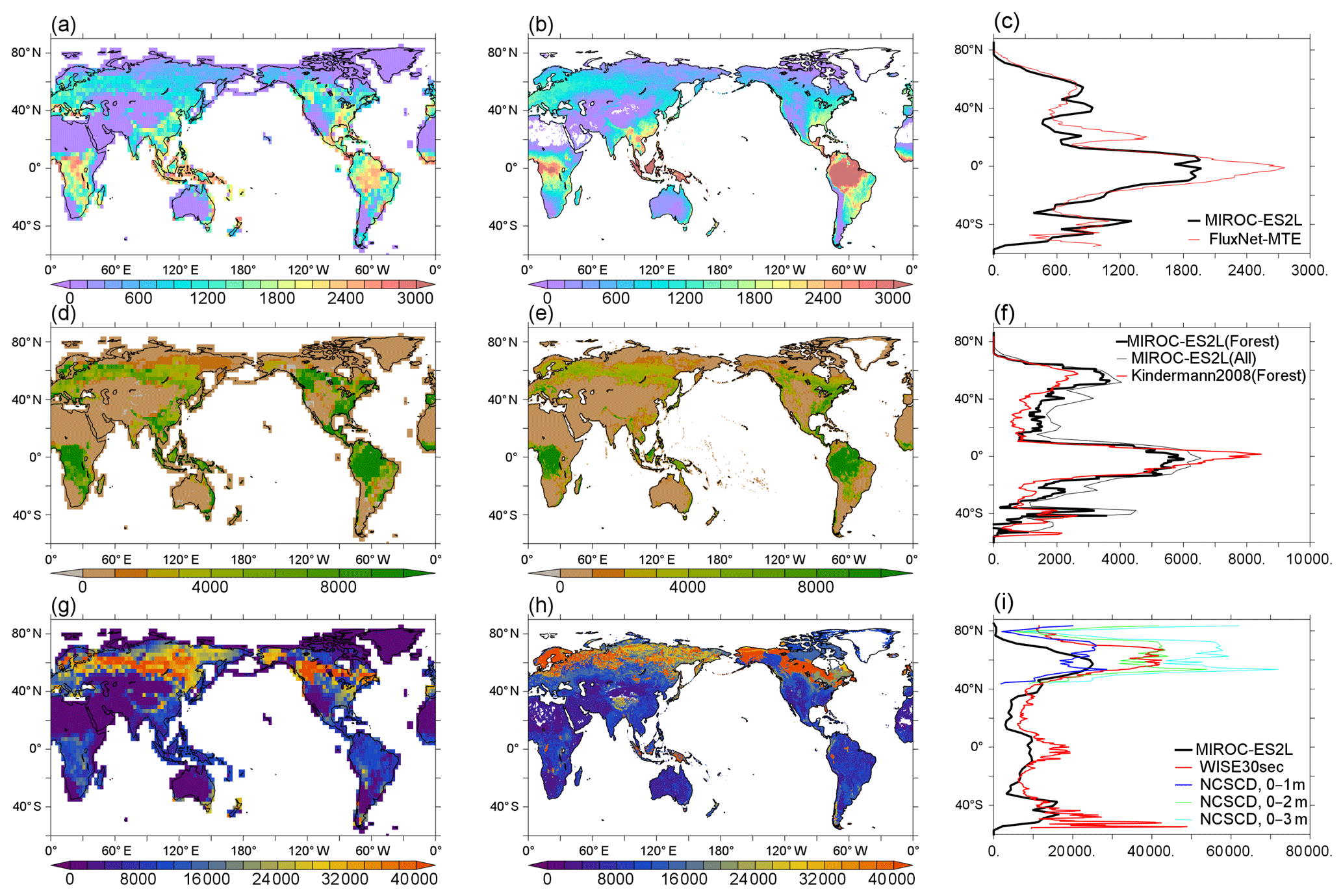
Figure 10 Comparison of the carbon flux and storage of the land ecosystem between the HIST simulation by MIROC-ES2L and an observation-based dataset. (a–c) A comparison of GPP (gC m⁻² yr⁻¹) averaged over 1982–2011: (a) model result, (b) FluxNet-MTE of Jung et al. (2011), and (c) zonally averaged distributions. (d–f) Vegetation carbon (gC m⁻²): (d) model result of forest carbon (obtained by masking the total vegetation carbon where forest coverage is <5 %), (e) forest carbon estimated by Kindermann et al. (2008), and (f) zonally averaged distributions; solid black and red lines represent forest carbon, and the dashed thin line is the total vegetation carbon simulated by the model. (g–i) SOC (gC m⁻²): (g) model result, (h) observation-based product of harmonized soil property values for broad-scale modeling (WISE30sec) by Batjes (2016), and (i) zonally averaged distributions in which the model result and WISE30sec are shown by black and red lines, respectively. Blue, green, and light blue lines in panel (h) are NCSCDv2 by Hugelius et al. (2013), which is an independent estimate of SOC in the high-latitude region of the Northern Hemisphere at different soil depths (blue: 0–1 m, green: 0–2 m, light blue: 0–3 m).

3.1.5 Ocean biogeochemistry

In this section, we evaluate the simulated surface and vertical distributions of nitrate, phosphate, dissolved Fe, NPP, oxygen, DIC, and alkalinity against observations (Fig. 11). Additionally, the ocean CO₂ flux is also compared with an observation-based estimation (Fig. 12). The observations comprise the World Ocean Atlas 2013 (WOA2013; Garcia et al., 2014a, b) for macronutrients and oxygen, the GEOTRACES dataset (updated to its 2015 version; Tagliabue et al., 2012) for dissolved iron, the Global Ocean Data Analysis Project version 2 (GLODAPv2; Lauvset et al., 2016) for DIC and alkalinity, and SeaWiFS (Behrenfeld and Falkowski, 1997) satellite observations for NPP.

Owing to the long spin-up, the drift in global averaged concentrations of biogeochemical tracers becomes close to zero. The linear drift of dissolved oxygen, NO₃, and Alk–DIC over the final 250 years of the spin-up is less than 3 % kyr⁻¹ (Supplement Table S3). This small bias is significant in providing results on ocean biogeochemistry and carbon cycle feedbacks that are quantitatively more correct (Séférian et al., 2016).

The simulated surface distributions of nitrate and phosphate are generally in agreement with the WOA2013 datasets (Fig. 11a and b). The surface macronutrient concentrations in HNLC regions (e.g., the Southern Ocean, North Pacific Ocean, and eastern equatorial Pacific Ocean) are higher than those produced by the ocean biogeochemical component of our previous model (Watanabe et al., 2011), and they are more consistent with the observed values. This increase in macronutrients in HNLC regions is reasonable because the implementation of the iron cycle and the iron limitation on phytoplankton growth can reduce macronutrient utilization in these regions. Ocean circulation also influences the distribution of nutrient concentrations. In the Southern Ocean, the deep mixed-layer depths simulated by the model can cause an overestimation of nutrient entrainment to the surface and thus produce a high nutrient bias (Fig. 7). The simulated global mean vertical profile of nitrate concentrations compares reasonably well with observed values, likely because the ocean circulation is represented adequately (Fig. 11a). To check the influence of ocean circulation on the tracer distributions, we compared the apparent oxygen utilization (AOU) between the model and observations (Supplement Fig. S10). Although the model captures the observed AOU distributions, the strong and deep AMOC causes an underestimation of AOU values in the Atlantic Ocean deep water. The largest bias is an underestimation in the North Pacific Ocean, which is caused by the strong deep circulation of the Pacific Ocean. It should be noted that the difficulty of simulating the Pacific Ocean deep circulation appears to be a general problem in present coarse-resolution models (Hasumi et al., 2010). Model–data agreement on vertical nitrate concentrations is also the result of the near balance between nitrogen cycle sources (i.e., nitrogen fixation, atmospheric nitrogen deposition, and riverine nitrogen input) and sinks (i.e., denitrification, N₂O emissions, and sedimentary loss) over the long spin-up period.

The concentration of dissolved iron in the open ocean is highest in the subtropical North Atlantic Ocean and in the Arabian Sea (Fig. 11c), which is consistent with the pattern observed in GEOTRACES. Such high concentrations are caused by enhanced dust deposition from the Sahara. In the remainder of the open ocean, dissolved iron concentrations are generally <0.2 µmol m⁻³, especially in HNLC regions. The model captures the main observed patterns in the surface ocean well. The very high iron concentrations (>1 µmol m⁻³) both observed and simulated along coasts and over continental margins are the result of iron input from sediment. The average simulated dissolved Fe concentration in the surface ocean (0–100 m) is 0.39 µmol m⁻³, which is lower than observed (0.52 µmol m⁻³) but within the range of the iron model intercomparison project (FeMIP; Tagliabue et al., 2016). One factor not accounted for in our model is the variation in the solubility of iron in aerosols, which depends not only on the source chemical composition but also on atmospheric processing during transport (Ito et al., 2019a). Consideration of different degrees of atmospheric Fe processing could reduce the overestimations of dissolved Fe concentration in the North Atlantic Ocean and North Pacific Ocean (Ito et al., 2019b). Our model also neglects variations in sedimentary iron flux. Observations have found that iron release or burial in sediment is dependent on the oxygen concentration of bottom water (Noffke et al., 2012), ambient temperature (Sanz-Lázaro et al., 2011), and the amount of OM that reaches the sea floor and is remineralized therein (Elrod et al., 2004). To simulate more realistic iron distributions, these processes should be considered in future studies.

Reproducing the spatial pattern of nutrient limitation on phytoplankton growth is crucial for the accurate prediction of primary production and for reflecting in the simulations the consequences of ongoing anthropogenic perturbations to oceanic nutrient cycles (Moore et al., 2013). The model reasonably reproduces the HNLC regions because of the iron limitation in the subarctic North Pacific Ocean, the equatorial Pacific Ocean, and the Southern Ocean (Supplement Fig. S11), although the subarctic North Pacific Ocean and the equatorial Pacific Ocean have larger HNLC zones than observed upwelling regions. This is likely because of an underestimation of surface iron concentrations and/or a relatively high half-saturation constant for iron uptake (Appendix B). Nitrogen limitation occurs throughout much of the low-latitude surface ocean where the nitrogen supply from the subsurface is relatively slow.

Based on the distribution pattern of nutrients and the limitations, annual NPP is simulated as 28.6 PgC yr⁻¹ (Table 4). This value is lower than a satellite-based estimate of 35–78 PgC yr⁻¹ (Carr et al., 2006), and it is also lower than the range of 30.9–78.7 PgC yr⁻¹ derived from the CMIP5 models (Bopp et al., 2013). This is likely attributable to the high half-saturation constant for iron uptake, as mentioned above. Although intense primary productivity in coastal regions is not resolved by the coarse grid, the modeled NPP agrees with the basin-scale patterns of observation-based NPP. The values of both modeled and observed NPP are high in regions of equatorial upwelling, the North Atlantic Ocean, and the Southern Ocean north of the polar front, whereas they are low in subtropical gyres (Fig. 11g). Global export production is estimated as 7.9 PgC yr⁻¹, which is the upper bound of the CMIP5 models (4.9–7.9 PgC yr⁻¹; Bopp et al., 2013).

The simulated surface distribution of dissolved oxygen compares reasonably well with observations (not shown). This is because the surface oxygen concentration is close to its solubility value, and it is strongly constrained by SST. At depth, oxygen minimum zones in the eastern equatorial Pacific Ocean, eastern tropical Atlantic Ocean, Arabian Sea, and Bay of Bengal are reproduced well (Fig. 11f). However, the model produces oxygen concentration values higher than observed; thus, it underestimates the hypoxic volume ([O₂] <80 mmol m⁻³) by a factor of 3 in comparison with data-based estimates (Bianchi et al., 2012). Note that existing global ocean biogeochemical models have difficulty in reproducing oxygen minimum zones owing to their coarse resolution and simple globally tuned parameterizations of vertical fluxes of OM (Cocco et al., 2013; Bopp et al., 2013). The positive bias in oxygen might be driven by wintertime mixing in the Southern Ocean and the North Pacific Ocean that is too intense (Fig. 7), which transports too much oxygen from the surface to depth.

The model also captures the global-scale patterns of observed DIC and alkalinity (Fig. 11d and e). High values of these tracers in subtropical gyres (and in the Southern Ocean for DIC) are found in the model output and observations. Salinity bias and the parameterization of calcium carbonate production in the model can contribute to the alkalinity bias. Overestimation of alkalinity in subtropical gyres leads to an overestimation of DIC because alkalinity affects the ocean's capacity to take up and store atmospheric CO₂.

Figure 12a shows the simulated annual mean air–sea CO₂ fluxes for the period 1985–2014 with observational estimates by Landschützer et al. (2014). Generally, the simulated spatial pattern is consistent with the data-derived estimates. The strongest carbon source to the atmosphere is found in the equatorial Pacific Ocean, and the most intense carbon sink is found in the North Atlantic Ocean. Model outgassing is weaker than the observational estimate in the North Pacific and equatorial Indian oceans. The model–data discrepancies are pronounced in the seasonal cycle of air–sea CO₂ fluxes in the Southern Ocean and the North Atlantic Ocean (Fig. 12b and c). In the Southern Ocean, the model simulates an opposite CO₂ flux seasonal phase, which could be driven by the bias in SST variability (Kessler and Tjiputra, 2016). In the North Atlantic Ocean, although the simulated seasonal phasing of CO₂ fluxes agrees with the observational estimate, the amplitude is overestimated. The processes driving the seasonal cycle should be investigated in future studies because simulating a proper regional seasonal cycle of air–sea CO₂ fluxes is important for future projections (Kessler and Tjiputra, 2016; Goris et al., 2018).

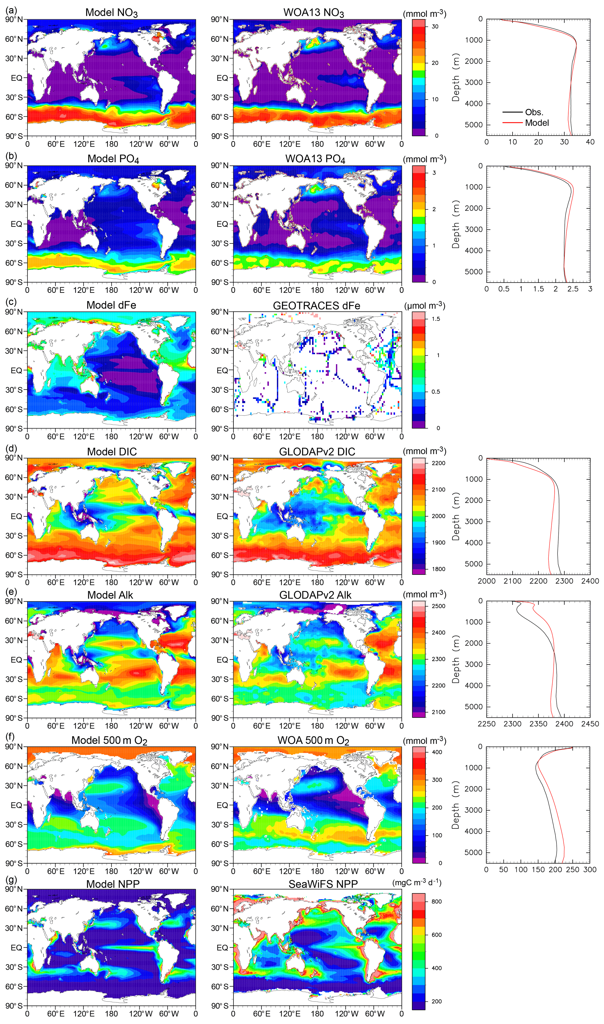
Figure 11 Comparison between model output and observations for key oceanic biogeochemical tracers. Simulated annual mean surface (a) nitrate, (b) phosphate, (c) DIC, (d) alkalinity, (e) dissolved oxygen at 500 m of depth, and (f) surface NPP for the 2000s are compared with observations from the WOA2013 (Garcia et al., 2014a, b) and GLODAPv2 datasets (Lauvset et al., 2016), as well as SeaWiFS (Behrenfeld and Falkowski, 1997) satellite observations. Left and central panels show the horizontal distributions of model output and observations. Right panels show the vertical distributions of model output (red lines) and observations (black lines).

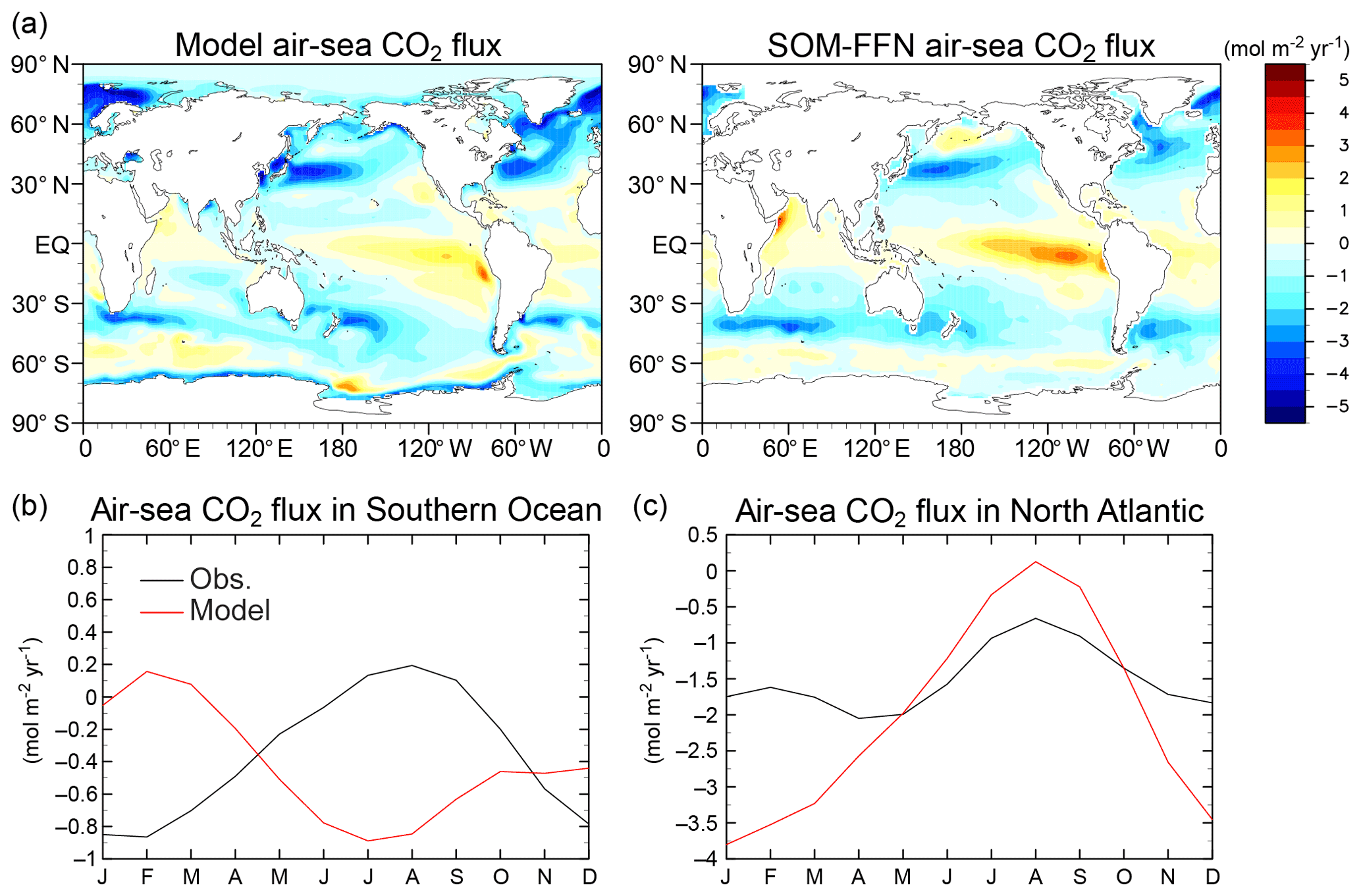
Figure 12 (a) Annual mean air–sea CO₂ fluxes from (left) the model and (right) observational estimates adopted from Landschützer et al. (2014). Seasonal cycle of air–sea CO₂ fluxes for (b) the Southern Ocean and (c) the North Atlantic Ocean. Red lines represent the model for the period 1985–2014, and black lines represent the observation-based estimates of Landschützer et al. (2014). Southern Ocean: 45–70^∘ S, North Atlantic Ocean: 30–70^∘ N.

3.2 Sensitivity analysis

3.2.1 Sensitivity of land biogeochemistry

To evaluate the sensitivities of modeled land biogeochemistry, we focus on GPP and its response to external forcing in the terrestrial system because this carbon flux is the primary driver of land carbon input. GPP change was calculated by taking the difference of the 2005–2014 averages between the HIST and CTL runs. Then, as diagnosed in Fig. 8c, the GPP change was decomposed into the response to (1) CO₂ increase, (2) climate change, and (3) LUC and agricultural change (Fig. 13) based on the simulation results of HIST, HIST-NOLUC, and HIST-BGC (Tables 1 and 2). Additionally, the GPP changes were further decomposed into the contributions from non-crop (i.e., the contribution of primary and secondary vegetation, urban areas, and pasture) and crop tiles by weighting the GPP of each tile by their areal fractions on a grid.

Figure 13d–f shows that CO₂ increase in the historical period is the main driver of change in the land carbon cycle and that the CO₂ fertilization effect prevails over most land areas except desert regions. Conversely, the GPP response to climate change shows both positive and negative signs (Fig. 13g–i) with relatively smaller magnitudes. Midlatitude and high-latitude regions of the Northern Hemisphere show a positive change in GPP that is likely attributable to lengthening of the vegetation growth season, enhanced plant growth following accelerated soil mineralization due to warming, and other mechanisms (e.g., soil water increase via precipitation and permafrost melting). In semiarid regions (i.e., Africa, South Asia, northern Australia, and the eastern side of South America), GPP shows a slight reduction. As these regions have less precipitation in comparison with the tropics, the reduction in GPP is likely associated with precipitation change.

In addition to the responses to CO₂ increase and climate change, the model demonstrates spatial variation in the response of GPP to LUC (Fig. 13j). Historical LUC reduces the non-crop GPP contribution (Fig. 13k), while the crop contribution is enhanced (Fig. 13l). In the tropics, LUC reduces the non-crop GPP but weakly increases crop GPP, which results in a net negative reduction of GPP as grid averages (Fig. 13j). Meanwhile, regions with intensive agriculture with nitrogen fertilizer input (e.g., western Europe, East Asia, and parts of North America) show a net positive change in GPP as grid averages, whereby increases in the crop contribution overcome reductions in the non-crop contribution (Figs. 13k and 12l). In the model, the crop contribution to GPP can be intensified by the following: (1) increasing the areal fraction of the crop tile following LUC forcing; (2) changing the vegetation type from natural vegetation to crop, whereby the latter has higher photosynthetic capacity than natural plant functional types (given as parameters that relate photosynthetic capacity to leaf nitrogen concentration; Appendix A); (3) applying nitrogen fertilizer to crop tiles; and (4) increasing nitrogen input via nitrogen-fixing crops, which is considered in the model to be a subcategory of crop tiles. Indeed, the total area of cropland increases in the 20th century in the HIST simulation (Supplement Fig. S2), which is reflected by the model producing an increase in nitrogen input via fertilizer application and biological fixation on the global scale (Fig. 9a).

By responding to CO₂ increase, climate change, and LUC, most land areas show increased GPP in the historical period (Fig. 13a), and regions with intensive agriculture show a greater increase in GPP than induced solely by the CO₂ fertilization effect (Fig. 13a and d). This suggests that modeled GPP is sensitive to land use and agricultural management forcing in addition to the increase in CO₂, and this might be one of the reasons for the slowing of LUC-induced land carbon reduction in the latter half of the 20th century in the HIST simulation (green line in Fig. 8c).

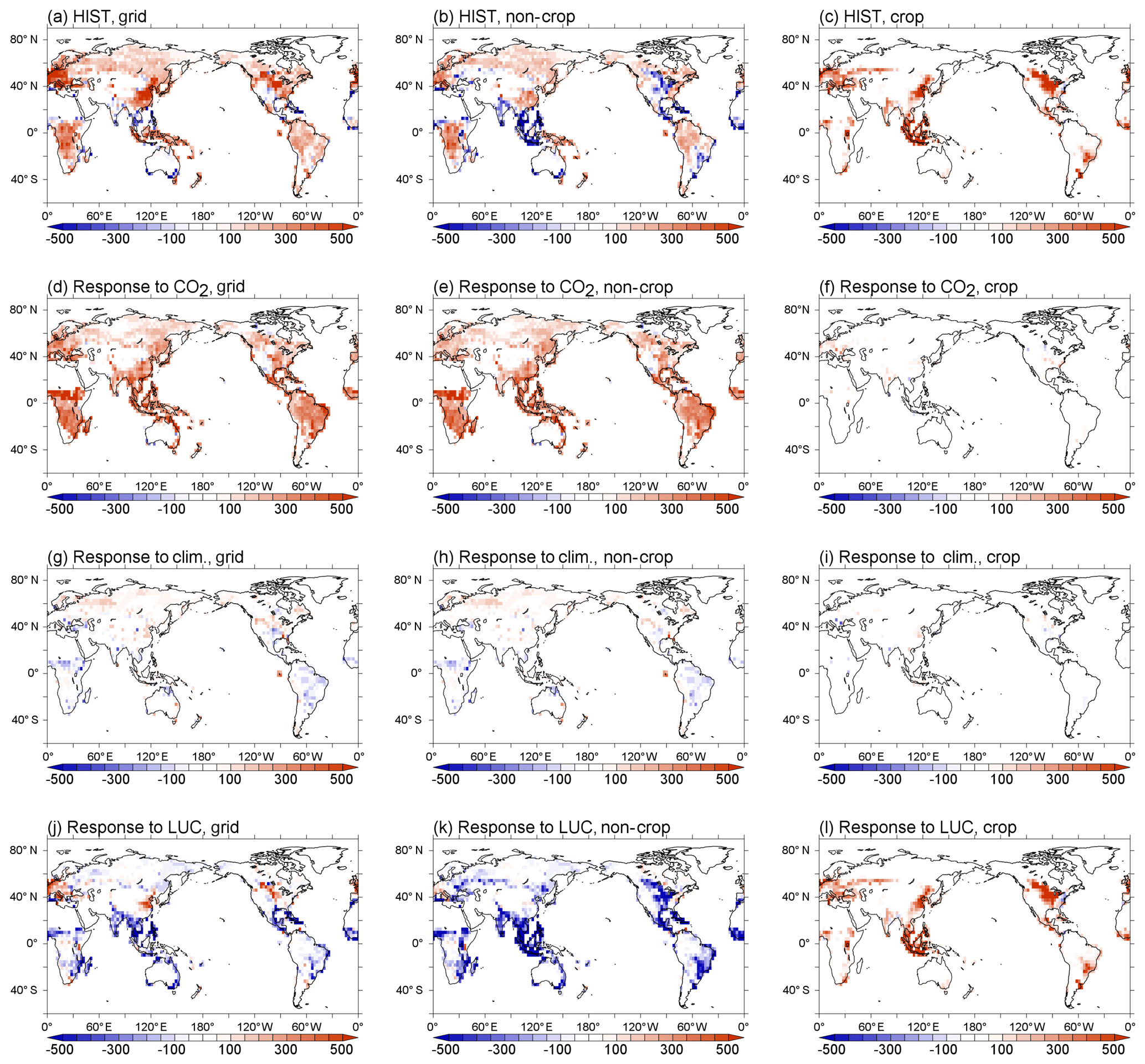
Figure 13 (a, b, c) Changes in GPP (gC m⁻² yr⁻¹) in HIST derived by taking the difference of the 2005–2014 averages of GPP between HIST and CTL. (d, e, f) GPP response to CO₂ increase diagnosed from simulation results of HIST, HIST-NOLUC, and HIST-BGC. (g, h, i) GPP response to climate change diagnosed by taking the difference between the simulation results of HIST and HIST-BGC. (j, k, l) GPP response to LUC obtained by taking the difference between HIST and HIST-NOLUC. GPP changes in each left-hand panel are further decomposed into contributions from (middle panels) non-crop tiles (primary vegetation, secondary vegetation, urban areas, and pasture) and (right-hand panels) crop tiles.

3.2.2 Sensitivity of ocean biogeochemistry

In this section, we investigate the sensitivity of oceanic NPP to external nutrient inputs from atmospheric deposition and river discharge processes under preindustrial conditions because these processes are newly incorporated into the ESM. Through the combination of the simulation results of CTL-D, NO-NR, NO-NRD, and NO-FD (Tables 1 and 2), the impacts of nutrient input on both the nutrient concentration and primary productivity are analyzed (Fig. 14 for N input assessment and Fig. 15 for Fe), and the spatial patterns of simulated nutrient limitation on NPP in the four experiments are examined (Fig. 16). Here, NO₃, Fe, and PO₄ limitation is diagnosed using the equations NO₃∕(kN + NO₃), Fe∕(kFe + Fe), and PO₄∕(kP + PO₄), respectively, as simulated in MIROC-ES2L (Eq. B17); Fig. 16 presents the strength of each limitation visualized by the intensity of each of the three primary colors (red, blue, and green). In the simulations, because changes in NPP and surface nutrient concentrations continued to change over several decades following the abrupt switching-off manipulation, the average over the final 10 years is used for the following analysis. The rapid response of NPP to changes in nutrient input is consistent with that found in previous research (Somes et al., 2016).

First, the impacts of riverine N input on the surface nutrient concentration and NPP are assessed by subtracting the zero-input scenario NO-NR from the control experiment CTL-D (Tables 1 and 2). Surface NPP is increased by riverine N input (by >10 gC m⁻³ yr⁻¹) in coastal areas such as the North Brazil Shelf and the Gulf of Mexico (Fig. 14a). In comparison with the pattern of the distribution of nutrient limitation (Fig. 16a and b), it is clear that a strong NPP increase in the open ocean occurs mainly in the Atlantic Ocean, which is under an N-limited condition. Conversely, NPP decreases in Fe-limited regions because the NPP increase in N-limited regions consumes surface dissolved Fe. Surface NO₃ concentrations increase only slightly in N-limited regions because NO₃ is immediately consumed locally by phytoplankton. A remarkable increase in surface NO₃ concentrations is found in Fe-limited regions such as the Kara Sea, North Atlantic Ocean, Hudson Bay, and Subantarctic Ocean. Global NPP increases by 0.7 PgC yr⁻¹ (by 2.5 % in comparison with NO-NR). This value is comparable with the finding of da Cunha et al. (2007), who estimated a 5 % increase in primary production due to riverine nutrient input. Note that nutrient retention in estuarine areas is not considered in our model. Thus, most nitrogen supplied from river mouths can easily be conveyed to the open ocean. Given that a recent modeling study estimated that approximately 75 % of riverine nitrogen globally escapes from shelf areas to the open ocean (Sharples et al., 2017), our results on the impact of riverine N on NPP should be viewed as an upper limit for the estimation.

Second, the effects of atmospheric N deposition on the surface nutrient concentration and NPP are evaluated by subtracting the zero-input scenario NO-NRD from the NO-NR experiment (Tables 1 and 2). Similar to riverine N input, atmospheric N deposition causes an increase in NPP in N-limited regions and a global increase in NO₃ (Figs. 14b, 16a and c). According to deposition flux, significant changes in NPP are found in coastal areas and low-latitude regions of the Pacific Ocean. Global NPP increases by 0.3 PgC yr⁻¹ (by 1 % in comparison with NO-NR), which is consistent with previous estimates (Duce et al., 2008; Moore et al., 2013).

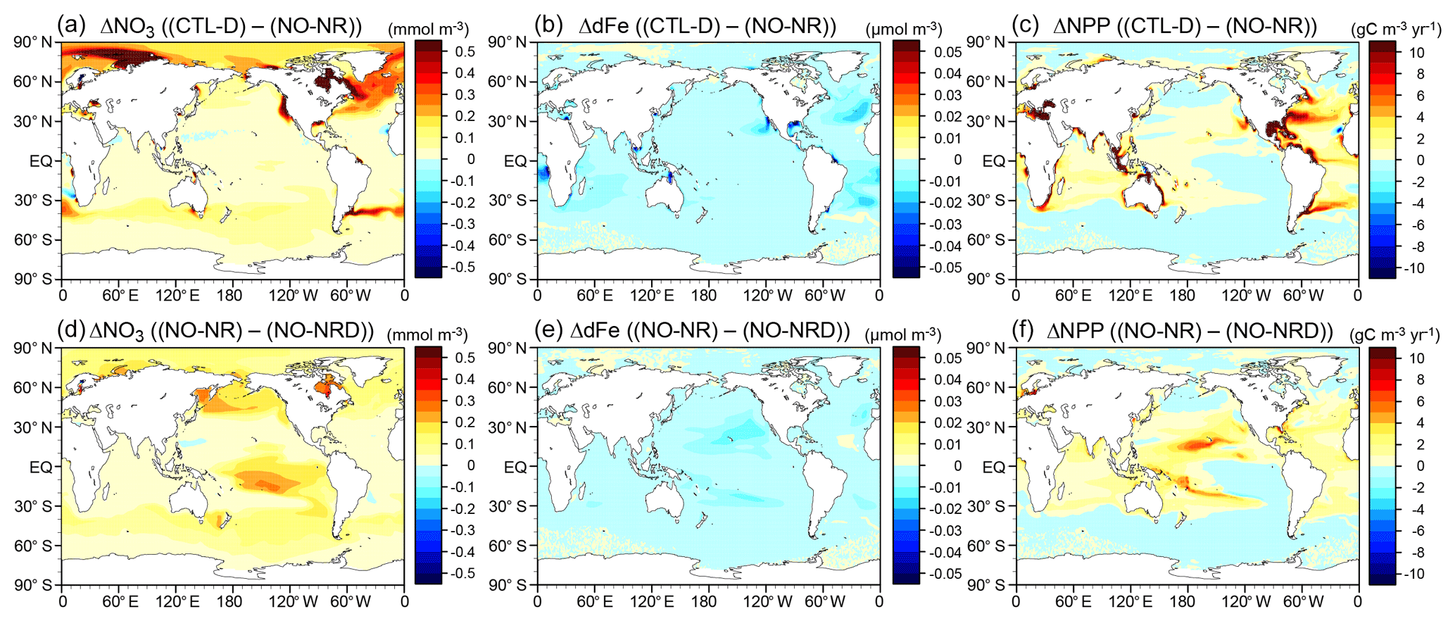
Figure 14 Changes in (a, d) surface nitrate, (b, e) dissolved iron, and (c, f) NPP driven by nitrogen input from (a–c) rivers (CTL-D – NO-NR) and (d–f) atmospheric deposition (NO-NR – NO-NRD).

Finally, changes in the surface nutrient concentration and NPP, driven by atmospheric Fe deposition, are calculated by subtracting the zero-input scenario NO-FD from the control experiment CTL-D (Tables 1 and 2). In contrast to N input, atmospheric Fe deposition causes an increase in NPP in Fe-limited regions and a decrease in N-limited regions (Figs. 15, 16a and d). A significant Fe increase is found in N-limited regions. Global NPP and export production increase by 1.8 and 0.8 PgC yr⁻¹, respectively (by 6.7 % and 11 %, respectively, in comparison with NO-FD). These percentage increases are consistent with previous estimations by Moore et al. (2013). However, the sensitivity of export production to Fe deposition from dust is higher than reported by Tagliabue et al. (2014), who estimated that export production increases by 0.06–0.11 PgC yr⁻¹. Therefore, it seems difficult to obtain robust sensitivity for both iron and the biological cycle to iron input because of the high uncertainty regarding the iron cycle among models. Although nitrogen input from both deposition and rivers has little effect on the spatial patterns of the distribution of nutrient limitation (Fig. 16a–c), iron input from the atmosphere changes the pattern in low-latitude regions from iron limitation to nitrogen limitation (Fig. 16a and d).

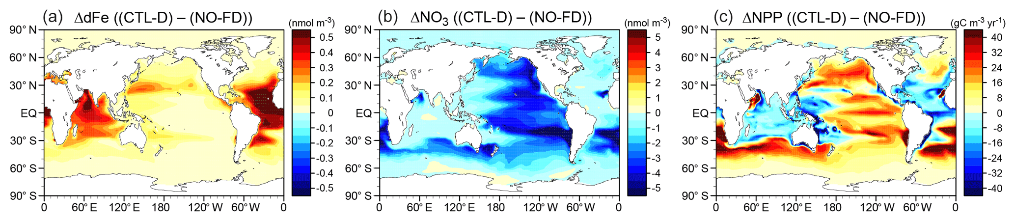
Figure 15 Changes in (a) surface dissolved iron, (b) nitrate, and (c) NPP driven by dissolved iron input from dust (CTL-D – NO-FD).

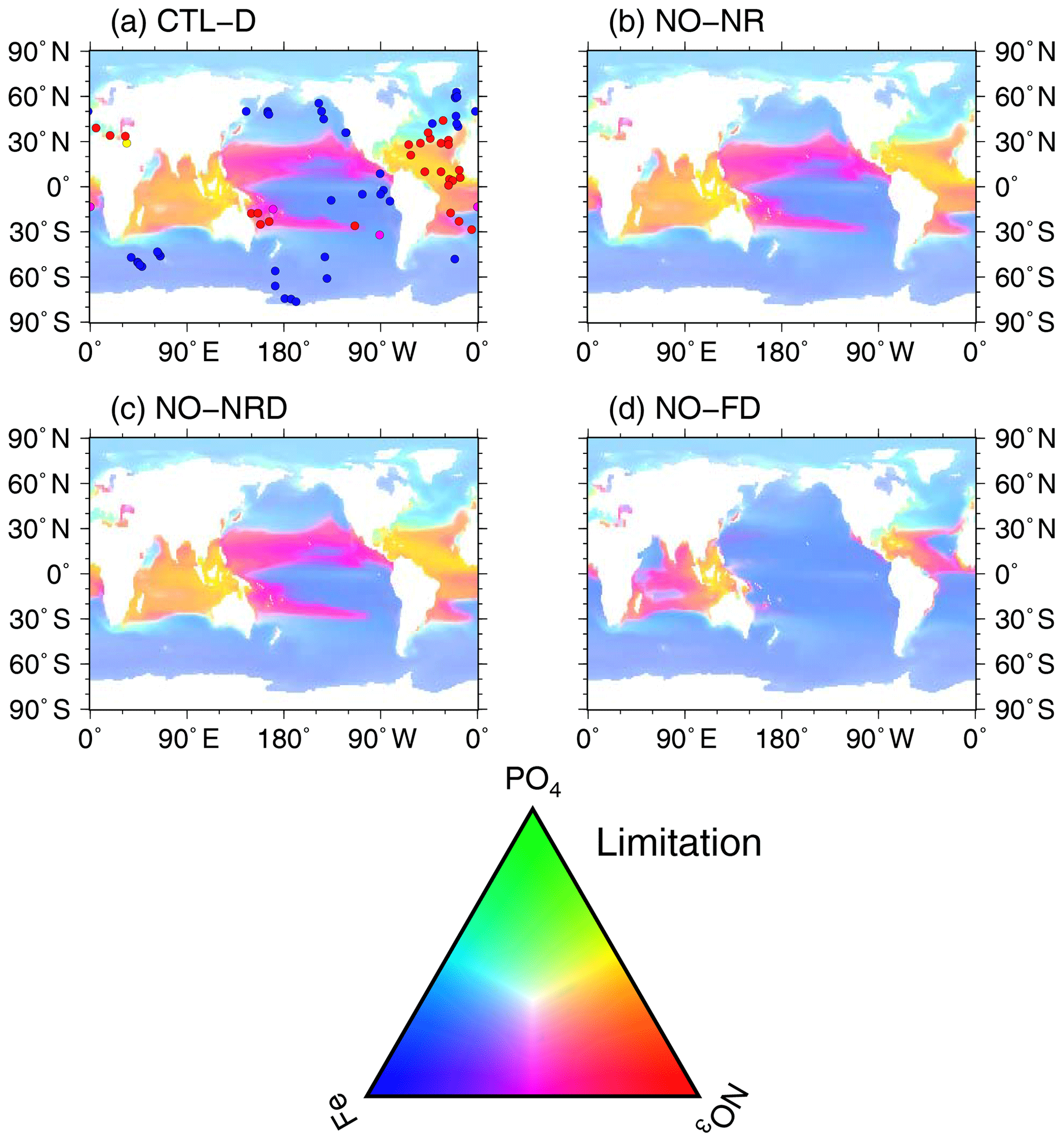
Figure 16 Limiting nutrient map for phytoplankton for (a) CTL-D, (b) NO-NR, (c) NO-NRD, and (d) NO-FD. Shading indicates limiting nutrient(s), e.g., red: N limitation, blue: Fe limitation, green: P limitation, magenta: N and Fe limitation, cyan: Fe and P limitation, yellow: P and N limitation (see bottom color triangle). Circles in (a) represent observed limiting nutrients from nutrient addition experiments (Moore et al., 2013).

Here, we examine model sensitivity against global inputs of both N and Fe into the ocean through atmospheric deposition and river discharge in the preindustrial condition. We note, however, that these two types of nutrient input have increased significantly since the preindustrial era because of human activities (Duce et al., 2008; Seitzinger et al., 2010; Krishnamurthy et al., 2010). Additionally, ongoing nutrient input increase can lead to a future increase in biological production, which might partly negate the production decrease driven by global warming. Conversely, the resultant increase in the export of OM would accelerate CO₂-induced ocean acidification and warming-induced deoxygenation in subsurface waters, which leads to major environmental pressures. Thus, the combined effects of global warming and anthropogenic nutrient input on ocean biogeochemical cycles should be explored in the future.

3.2.3 Sensitivity of riverine nitrogen

The coupling of land and ocean ecosystems via riverine nitrogen is one of the new features of MIROC-ES2L, and the potential impact of the process on ocean biogeochemistry has already been examined and discussed in Sect. 3.2.2. Here, we examine the response of river nitrogen loading itself against anthropogenic forcing by comparing the results of the CTL, HIST-NOLUC, and HIST simulations. As mentioned in Sect. 3.1.3, the global flux of riverine nitrogen input into the ocean is simulated at 17.5 TgN yr⁻¹ in the CTL experiment (Table 4), and the flux is almost doubled in the 2000s at 33.9 TgN yr⁻¹ in the HIST run. This number is larger than previous estimates of 19–25 TgN yr⁻¹ for the present-day condition (Smith et al., 2003; Mayorga et al., 2010; Dumont et al., 2005). This overestimation might be caused by the inability of the model to simulate all forms of nitrogen in rivers. For example, the model simulates only the dissolved inorganic nitrogen (DIN) flux; thus, the expected nitrogen flux with non-DIN forms (e.g., dissolved organic and particulate matter) might be partly imposed on the DIN flux in the simulations. Indeed, the global total nitrogen flux, including DIN, dissolved organic nitrogen, and particulate nitrogen, is estimated at 37–66 TgN yr⁻¹ (Beusen et al., 2016; Mayorga et al., 2010; Boyer et al., 2006; Seitzinger et al., 2005), which is closer to the result of MIROC-ES2L.

Another possible reason for the above overestimation is precipitation bias, which results in the overestimation of BNF on land. As mentioned in Sect. 3.1.1, the model has a positive precipitation bias on land in arid and desert regions (Supplement Fig. S6). As the scheme for the natural BNF flux employed in MIROC-ES2L is modeled to be controlled by the actual evapotranspiration rate (Cleveland et al., 1999), the precipitation bias in arid regions could easily lead to an overestimation of the BNF flux and an increase in riverine nitrogen loading. This is also evident when decomposing the global riverine flux into river basins and comparing the findings with a previous study by Dumont et al. (2005) (Fig. 17). MIROC-ES2L overestimates the DIN fluxes of large rivers such as the Amazon, Mississippi, and Yangtze rivers, even in the CTL experiment, in which all anthropogenic forcings are fixed at preindustrial levels. This suggests the necessity of improvement of the baseline flux of riverine nitrogen in the model. For more in-depth discussion, it will be necessary to explicitly simulate the organic and particulate nitrogen fluxes in rivers, and it might be necessary to simulate the explicit sedimentary and chemical reaction processes in freshwater and coastal zone systems.

In Fig. 17, the difference between the results of CTL and HIST-NOLUC mainly reflect the change induced by nitrogen deposition (and historical climate change) (Table 2), and the model demonstrates that deposition has increased N fluxes in many rivers. Additionally, the difference between HIST-NOLUC and HIST demonstrates the impact of LUC and agricultural management change (Table 2), and regions that have intensive agriculture within their watersheds (e.g., the basins of the Mississippi, Indus, Yellow, and Yangtze rivers) are simulated as strongly affected by the forcing change. The DIN discharge in each river is not always smaller in HIST-NOLUC than in HIST. This is because LAI in HIST-NOLUC is different to that in HIST, which is sometimes accompanied by a slight change in the surface climate via biophysical feedback. If the soil temperature is slightly warmer in HIST-NOLUC than in HIST, the soil mineralization rate in HIST-NOLUC should be accelerated, and thus the DIN loadings of rivers could be increased. This simulated trend in the historical period is qualitatively consistent with previous studies (Gruber and Galloway, 2008). Furthermore, the model simulates the global riverine flux to be increased by 16.4 TgN yr⁻¹ in the historical period. This value is quantitatively consistent with previous estimates, e.g., 16 TgN yr⁻¹ by Dumont et al. (2005) for DIN flux and 18 and 19 TgN yr⁻¹ by Beusen et al. (2016) and by Green et al. (2004), respectively, for total N flux. Although bias exists in the magnitude of riverine nitrogen flux both globally and locally, we confirm that the model can qualitatively capture the changes in riverine nitrogen flux during the historical period.

Figure 17 Simulated and observed DIN load per river basin: sorted by simulated (a) first 10 largest rivers and (b) second 10 largest rivers. Vertical gray bars represent observations (Dumont et al., 2005); blue, green, and yellow bars correspond to the results of the HIST, HIST-NOLUC, and CTL experiments, respectively.

3.2.4 TCR, AF, and TCRE

Here, the model sensitivity of the global climate–carbon cycle against CO₂ increase is analyzed by calculating TCR, AF, and TCRE from the results of the 1PPY, 1PPY-BGC, and 1PPY-RAD experiments (see Sect. 2.2.2 for the method). These quantities summarize the total performance of the climate, carbon cycle, and coupled climate–carbon cycle system in the models, which enables us to compare them with existing ESMs.

The TCR, AF, and TCRE derived from the 1PPY simulation are displayed in Table 5. The TCR of MIROC-ES2L is 1.5 K, which is lower than the multimodel mean of the CMIP5 ESMs but within the range of spread (1.8±0.5 K; Gillet et al., 2013). Compared with our previous ESM (i.e., MIROC-ESM; Watanabe et al., 2011), the TCR has decreased by 32 % because of the replacement of the physical core of the ESM from the MIROC3-based model to that of MIROC5 (Watanabe et al., 2010). The value of AF, which is a quantity that characterizes the carbon cycle response in an ESM but is dependent on TCR, was simulated at 0.61 in MIROC-ESM. This value is reduced to 0.52 in MIROC-ES2L; i.e., the new model has a stronger carbon sink than the previous version. The value of AF in the new model is of similar magnitude to the CMIP5 model average (0.53±0.06; Gillet et al., 2013). The lowered TCR and the moderate AF cause the new model to have moderate TCRE (1.3 K EgC⁻¹), which is smaller than that of the CMIP5 model average (1.6±0.5 K EgC⁻¹) by 19 %. Using TCRE, we can approximate the value of CE until the global temperature exceeds a specific mitigation target; CE for the 2 ^∘C warming target should be approximately 1540 PgC for MIROC-ES2L, 910 PgC for MIROC-ESM, and 950–1820 PgC for the CMIP5 models.

Table 5 Comparison of TCR, AF, and TCRE between MIROC-ES2L, MIROC-ESM, MIROC5.2, and CMIP5 ESMs in the 1PPY simulation. For MIROC-ES2L, both TCR and AF are calculated based on 20-year means of T2, CL, and CO centered on the 70th year of the 1PPY simulation (i.e., the time when the CO₂ concentration is doubled from the preindustrial condition), and TCRE is calculated based on TCR and AF. Numbers for the CMIP5 ESMs were obtained from Gillett et al. (2013) and are presented as the multimodel mean ±1σ.

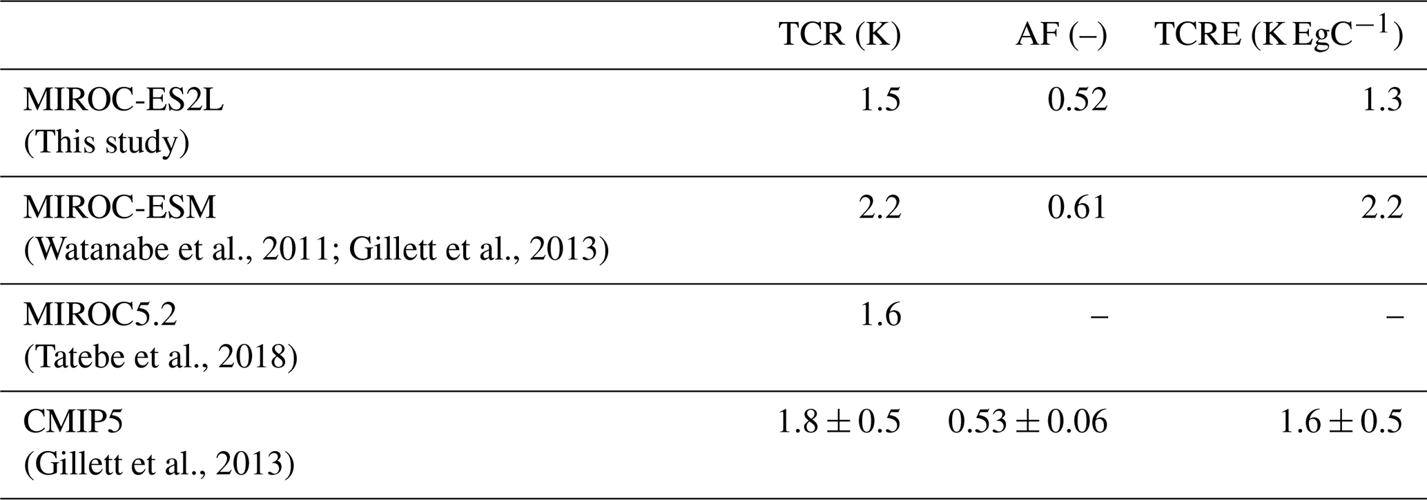
To further explore why AF is lowered in MIROC-ES2L, the strengths of the carbon cycle feedbacks were analyzed using the 1PPY-BGC and 1PPY-RAD simulation results (Table 6), and the findings were compared with the CMIP5 ESMs (Arora et al., 2013). The strength of the CO₂–carbon feedback (β) of land is simulated to be 0.52 PgC PgC⁻¹, which is slightly higher than the CMIP5 model average (0.43±0.21 PgC PgC⁻¹) and larger than that of MIROC-ESM by 48 %. The strength of oceanic CO₂–carbon feedback in the CMIP5 ESMs displays less spread among the models (0.38±0.03 PgC PgC⁻¹), and the result of MIROC-ES2L is within this spread (0.35 PgC PgC⁻¹). The absolute magnitude of the climate–carbon feedback (γ) for land and ocean in MIROC-ES2L is −71 and −4.5 PgC K⁻¹, respectively, both of which are less negative than the result of MIROC-ESM by 20 % for land and 63 % for ocean. Consequently, the land γ in MIROC-ES2L is within the range of the CMIP5 ESMs ($-\mathrm{58}\pm \mathrm{29}$ PgC K⁻¹), while the ocean γ is slightly larger than the upper range of the CMIP5 ESMs ($-\mathrm{7.8}\pm \mathrm{2.9}$ PgC K⁻¹).

As the quantities β and γ have different units, it is difficult to conclude which feedback process contributes most to the AF change. To compare them with the same unit, we used the quantity u proposed by Gregory et al. (2009). This quantity, which is defined as u_β=β and $u_{\mathit{\gamma }}=\mathit{\gamma }\times T/\mathrm{CA}$ (PgC PgC⁻¹), can relate the carbon cycle feedback parameters to AF, as AF $=\mathrm{1}/(\mathrm{1}+u_{\mathit{\beta }\mathrm{L}}+u_{\mathit{\beta }\mathrm{O}}+u_{\mathit{\gamma }\mathrm{L}}+u_{\mathit{\gamma }\mathrm{O}})$ (see Appendix E for the derivation). When comparing the u quantities of MIROC-ES2L with the CMIP5 models (Fig. 18), it is evident that the ocean component of MIROC-ES2L is less sensitive than the previous model for both CO₂–carbon and climate–carbon feedbacks. These two changes almost counteract each other; thus, the ocean component does not explain the reduced AF in the new model (Table 5). For land, the climate–carbon feedback (u_γ) in MIROC-ES2L is intermediate, while MIROC-ESM was one of the most sensitive models of the CMIP5 ESMs. Additionally, the magnitude of the land CO₂–carbon feedback (u_β) is increased from MIROC-ESM to MIROC-ES2L by 48 % (u_β=β). Therefore, the land component is the main cause of the lower AF, making the magnitude of both the CO₂–carbon and the climate–carbon feedbacks more positive and less negative, respectively, i.e., strengthening the land carbon sink.

Table 6 Comparison of CO₂–carbon and climate–carbon feedback parameters between MIROC-ES2L, MIROC-ESM, and the CMIP5 ESMs. As presented in Arora et al. (2013), TCR, AF, and TCRE are calculated at the time when the CO₂ concentration is quadrupled from the preindustrial condition (i.e., the 140th year in the 1PPY simulation) by taking the anomaly from the CTL run. Numbers for CMIP5 ESMs were obtained from Arora et al. (2013) and are presented as the multimodel mean ±1σ.

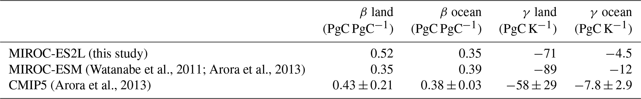
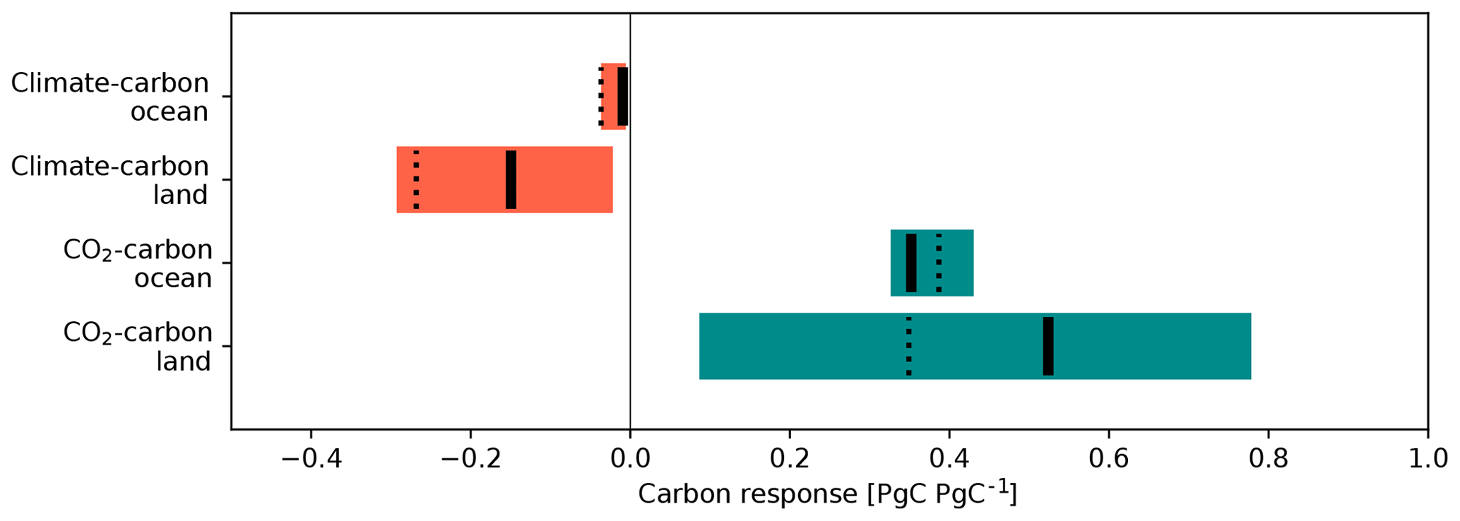
Figure 18 Comparison of the strength of CO₂–carbon and climate–carbon feedbacks between MIROC-ES2L and the CMIP5 models evaluated using the 1PPY, 1PPY-BGC, and 1PPY-RAD experiments. Vertical solid and dotted black bars represent MIROC-ES2L and MIROC-ESM, respectively, and the horizontal bars represent the range of the CMIP5 ESMs (mean ±1.65σ). To compare the two types of feedback strength with the same unit, land and ocean carbon storage change were both normalized by dividing the atmospheric carbon change, which corresponds to the u quantity proposed by Gregory et al. (2009): CE = CA ($\mathrm{1}+u_{\mathit{\beta }}+u_{\mathit{\gamma }}$), where u_β=β, $u_{\mathit{\gamma }}=\mathit{\gamma }\times \mathit{\alpha }$. If u>0 (u<0), the feedback sign is negative (positive). The calculations were based on the anomaly from the CTL run at the time of a quadrupled CO₂ concentration from the preindustrial condition (i.e., the 140th year of the 1PPY, 1PPY-BGC, and 1PPY-RAD simulations).

4 Summary and conclusions

In this study, a new Earth system model (MIROC-ES2L) was developed using a state-of-the-art climate model (MIROC5.2) as the physical core. This new ESM embeds a terrestrial biogeochemical component with explicit carbon–nitrogen interaction (VISIT-e) that accounts for the nutrient limitation of nitrogen on plant growth and therefore the change in the land carbon fluxes. Additionally, the ocean biogeochemical component (OECO2) is largely updated to simulate the biogeochemical cycles of carbon, nitrogen, phosphorus, iron, and oxygen such that oceanic primary productivity in the model is now controlled by multiple nutrient limitations. As a new challenge, land and ocean nitrogen cycles were coupled via river discharge processes; thus, marine productivity is now also affected by the riverine nitrogen input. Furthermore, iron-related processes such as emission, atmospheric transport, deposition, and utilization in the marine ecosystem are newly included to represent the micronutrient limitation on phytoplankton productivity. This is necessary to reproduce the HNLC regions and simulate ecosystem variability in response to changes in external iron inputs.

To evaluate the performance of the new model, a historical simulation following CMIP6 protocols and forcing datasets was performed for the 1850–2014 period, and the results were compared with observation-based products. The model reasonably reproduces the global changes in net TOA radiation balance, SAT, SST, and upper-ocean temperature. Considering the few biophysical feedbacks on climate in the model, the MIROC-ES2L good performance in simulating the physical fields is inherited from its original climate model (MIROC5.2), although persistent problems remain such as the warm bias in the Southern Ocean, as found in some climate models. Global carbon and nitrogen budgets in the historical simulation were also examined and discussed by comparing the results with existing studies. The model successfully captured the observation-based estimates of contemporary air–sea and air–land carbon fluxes in terms of cumulative values. The component fluxes of global nitrogen between land, atmosphere, and ocean are also reasonably reproduced by the model. The spatial distributions of fundamental variables of the land carbon cycle were also assessed through comparison with observation-based products, and the model produced reasonable patterns for primary productivity, forest carbon, and SOC. The spatial patterns of oceanic macronutrients and micronutrients, total inorganic carbon, alkalinity, oxygen, primary productivity, and oceanic CO₂ flux were all captured well in the historical simulation.

To assess the global climate–carbon cycle feedback in MIROC-ES2L, a sensitivity analysis was performed in which the atmospheric CO₂ concentration was prescribed to increase by 1 % yr⁻¹. Then, the values of TCR, AF, and TCRE were calculated and compared with those of the CMIP5 ESMs. TCR in the new model is reduced to 1.5 K, which is approximately 70 % of the previous model used for CMIP5, through the replacement of the physical core from the MIROC3-based model to that of MIROC5.2. AF is also reduced by 15 %. Further feedback analysis of the carbon cycle revealed that most of the AF reduction should be attributable to the intensified land carbon sink in the new model, which results in a level of AF that is close to the average of the CMIP5 ESMs. TCRE, which is a quantity that aggregates the temperature response as a result of the entire climate–carbon cycle processes against anthropogenic CO₂ emissions, is 1.3 K EgC⁻¹ in MIROC-ES2L. This is reduced from the value seen in the model used for CMIP5 by 32 %, and it is slightly smaller than the multimodel mean of the CMIP5 ESMs. Thus, MIROC-ES2L might be an “optimistic” model in terms of simulating global climate and carbon cycle change considering that some CMIP6-class models are likely to have higher climate sensitivity (Voosen, 2019). A multimodal comparison of feedback strengths using CMIP6 ESMs is necessary to clarify whether the climate and carbon cycle sensitivities in MIROC-ES2L are realistic and to establish constraints on each feedback process based on observations (e.g., Wenzel et al., 2016; Goris et al., 2018).

In the new model, the terrestrial nitrogen cycle processes and the interaction with the carbon cycle are modeled explicitly. By performing several types of simulations, it was clearly demonstrated that agricultural management such as fertilizer application has changed the carbon cycle (GPP) in the historical period, which suggests that the nitrogen cycle in the model alters the land carbon cycle. The model simulated the change in the total land carbon content during 1850–2014 at 44 PgC, which is within the estimated range of Le Quéré et al. (2018). However, historical terrestrial carbon change is highly uncertain because the change is processed by multiple responses against the external forcing of CO₂, LUC, and climate change, each of which has its own estimation uncertainty. Thus, as performed in this study, decomposition of the impact of these forcings in historical simulations and in multimodel comparisons would be helpful in specifying the processes that produce the large simulation spread of the land carbon budget among the ESMs. Furthermore, although we confirmed that the nitrogen cycle alters the carbon cycle in the model, this study did not quantify the extent to which the soil nutrient deficit could downregulate plant growth and reduce the natural carbon sink. For this, a sensitivity analysis associated with carbon–nitrogen interaction is planned in CMIP6 (Jones et al., 2016), and the multimodel comparison study will reveal the strength of the carbon–nitrogen feedback in MIROC-ES2L relative to other CMIP6-class ESMs.

In the new model, the ocean nitrogen cycle is modified to be an open system, and thus the model can reflect the influences of external sources of nitrogen via atmospheric deposition and river discharge. Our sensitivity analyses under the preindustrial condition suggested minor contributions of these two external sources to primary productivity on the global scale. However, regions in which primary productivity is constrained by nitrogen availability showed a strong positive NPP response to the relaxation of nitrogen limitation. It accelerates the use of other nutrients within the marine ecosystem in such regions and reduces iron and phosphorus availability in other regions. Furthermore, by switching on the process of iron deposition into the ocean, the model showed an increase of approximately 7 % in primary production under the preindustrial condition, which suggests that iron input has a relatively stronger impact than nitrogen. Coupling iron cycle processes in the model led to the successful reproduction of HNLC regions, and it will enable the model to project future biogeochemical changes induced by anthropogenic iron emissions associated with the use of fossil fuels and biomass burning. We note, however, that as an atmospheric chemistry module is not included in MIROC-ES2L, the atmospheric chemical reaction of iron-containing aerosols is ignored and the iron solubility to seawater is simply assumed constant. Considering the relatively strong impact of iron deposition on marine primary productivity in the model, we need further detailed evaluation and modification of the iron cycle processes in terms of both aerosol transport and marine biogeochemical responses.

In addition to such improvements in terms of the iron cycle, other factors should also be improved and extended in the ESM for future simulation study. First, a freshwater biogeochemistry module is required. In the present model, the chemical form of riverine nitrogen is assumed inorganic, but actual river flow contains OM and particulate matter that undergo biogeochemical processing during transport. Thus, inclusion of the transport of organic–inorganic matter and the modeling of freshwater biogeochemistry might be necessary. This conclusion is supported by the sensitivity analysis that showed a relatively strong regional-scale impact of riverine nitrogen on marine primary productivity, although the global-scale impact was demonstrated to be minor. Second, MIROC-ES2L can simulate natural emissions of nitrous oxide; however, the emissions did not change the radiative balance in the atmosphere. Nitrous oxide is one of the strongest greenhouse gases with a long lifetime. As diagnosed in this study, future nitrous oxide emissions could be controlled by land use and agriculture, as well as climate change. Therefore, full coupling of the nitrous oxide cycle with other associated atmospheric chemical processes should be incorporated in the next-generation ESM, together with the methane cycle, as suggested in previous studies (e.g., Collins et al., 2018). Third, a mechanistic model for the denitrification process in ocean sediment should be included in a future model. The present model simulates only the denitrification rate of the water column, and the flux from sediment is likely imposed on the water-column denitrification. As the timescale of the sedimentary process is likely longer than that of water-column denitrification, explicit modeling of sedimentary denitrification will be important, particularly for long-term simulations over timescales of millennia. Finally, we partly demonstrated the importance of external sources of nutrients for marine productivity, although its evaluation was performed under the preindustrial condition. As anthropogenic nutrient inputs under that condition are much smaller than under the present-day condition and could be amplified or mitigated in the future, a similar set of sensitivity simulations should be undertaken for present-day and future conditions.

ESMs represent powerful tools to investigate interactions between the climate, biogeochemistry, and human activities, and they have facilitated climate projections and quantifications of future emissions of greenhouse gases for achieving climate change mitigation goals. Such models are also valuable for examining how Earth system components might respond to different levels of mitigation policies and scenarios spanning from the business-as-usual scenario to one employing intensive measures such as geoengineering techniques. Furthermore, state-of-the-art ESMs can reproduce some of the dominant long-term environmental changes on Earth that are becoming evident or doubted in association with climate change, e.g., ocean acidification and hypoxia, global nitrogen loading, air pollution, and habitable zone changes in ecosystems. ESMs can simulate such problems and their interactions in a holistic and consistent manner. Such simulations have the potential to elucidate sustainable ways to mitigate climate change with less environmental stress. To support such applications, further efforts should be made to improve ESMs and to constrain model performance in collaboration with observation studies.

Appendix A: Land ecosystem–biogeochemical component

A1 Nitrogen cycle

The structure of carbon and nitrogen compartments and the flux calculations in VISIT-e mostly follow the original version of the model (Ito and Inatomi, 2012a). For N cycle and LUC processes, some major changes were brought to VISIT-e to couple the model with MIROC-ES2L; the details are described below.

A1.1 N compartment structure in VISIT-e

Terrestrial N dynamics in VISIT are simulated based on three major compartment groups of N storage: vegetation N (N_VEG), soil organic matter (N_SOM), and soil inorganic matter (N_IOM). The component N_VEG is composed of canopy N (N_CAN) and storage N (N_STG):

$$N_{\mathrm{VEG}}=N_{\mathrm{CAN}}+N_{\mathrm{STG}}.$$

The mass conservation equations for N_CAN and N_STG are as follows:

$$\begin{array}{}\text{(A1)}& {\displaystyle }\begin{array}{rl}& \mathrm{d}{N}_{\mathrm{CAN}}/\mathrm{d}t={\mathrm{FN}}_{\text{SBNF, CAN}}+{\mathrm{FN}}_{\text{UPTK, CAN}}+{\mathrm{FN}}_{\text{RALC}}\\ & -{\mathrm{FN}}_{\text{MORT, CAN}},\end{array}\text{(A2)}& {\displaystyle }\begin{array}{rl}& \mathrm{d}{N}_{\mathrm{STG}}/\mathrm{d}t={\mathrm{FN}}_{\text{SBNF, STG}}+{\mathrm{FN}}_{\text{UPTK, STG}}+{\mathrm{FN}}_{\text{WTHD}}\\ & -{\mathrm{FN}}_{\text{MORT, STG}},\end{array}\end{array}$$

where FN represents nitrogen flux, and the subscripts SBNF, UPTK, RALC, WTHD, and MORT represent symbiotic biological N fixation, N uptake by plants, reallocation of storage N to the canopy, withdrawal of canopy N to storage, and loss of N by mortality, respectively. In this study, biological N input into vegetation (represented by FN_SBNF) is modified from the original model; the details are described in Sect. A1.2.

The component N_SOM is composed of the three nitrogen pools of litter (N_LIT), humus (N_HUM), and microbes (N_LIT):

$$\begin{array}{}\text{(A3)}& N_{\mathrm{SOM}}=N_{\mathrm{LIT}}+N_{\mathrm{HUM}}+N_{\mathrm{MCR}}.\end{array}$$

The N conservation equations for the pools are as follows:

$$\begin{array}{}\text{(A4)}& {\displaystyle }\begin{array}{rl}& \mathrm{d}{N}_{\mathrm{LIT}}/\mathrm{d}t={\mathrm{FN}}_{\text{MORT, CAN}}+{\mathrm{FN}}_{\text{MORT, STG}}+{\mathrm{FN}}_{\mathrm{NBNF}}\\ & -{\mathrm{FN}}_{\mathrm{HUMF}}-{\mathrm{FN}}_{\text{MNRL, LIT}},\end{array}\text{(A5)}& {\displaystyle }\begin{array}{rl}& \mathrm{d}{N}_{\mathrm{HUM}}/\mathrm{d}t={\mathrm{FN}}_{\mathrm{HUMF}}+{\mathrm{FN}}_{\text{MORT, MCR}}\\ & -{\mathrm{FN}}_{\text{MNRL, HUM}},\end{array}\text{(A6)}& {\displaystyle }\mathrm{d}{N}_{\mathrm{MCR}}/\mathrm{d}t={\mathrm{FN}}_{\text{IMBL}}-{\mathrm{FN}}_{\text{MORT, MCR}},\end{array}$$

where the subscripts NBNF, HUMF, MNRL, and IMBL represent nonsymbiotic BNF, humification of litter, mineralization of litter and humus, and immobilization by microbes, respectively. The components FN_NBNF and FN_HUMF are new components of flux, which are described in Sect. A1.2 and A1.3, respectively.

The inorganic nitrogen is assumed to consist of N pools of ${\mathrm{NH}}_{\mathrm{4}}^{+}$ ($N_{{\mathrm{NH}}_{\mathrm{4}}}$) and ${\mathrm{NO}}_{\mathrm{3}}^{-}$ ($N_{{\mathrm{NO}}_{\mathrm{3}}}$):

$$\begin{array}{}\text{(A7)}& {\displaystyle }{N}_{\mathrm{IOM}}=N_{{\mathrm{NH}}_{\mathrm{4}}}+N_{{\mathrm{NO}}_{\mathrm{3}}}.\end{array}$$

The budget equation for $N_{{\mathrm{NH}}_{\mathrm{4}}}$ is as follows:

$$\begin{array}{}\text{(A8)}& \begin{array}{rl}& \mathrm{d}{N}_{{\mathrm{NH}}_{\mathrm{4}}}/\mathrm{d}t={\mathrm{FN}}_{\mathrm{DEPO},{\mathrm{NH}}_{\mathrm{4}}}+{\mathrm{FN}}_{\mathrm{FRTL},{\mathrm{NH}}_{\mathrm{4}}}\\ & +{\mathrm{FN}}_{\text{MNRL, LIT}}+{\mathrm{FN}}_{\text{MNRL, HUM}}-{\mathrm{FN}}_{\mathrm{UPTK},{\mathrm{NH}}_{\mathrm{4}}}\\ & -{\mathrm{FN}}_{\text{IMBL}}-{\mathrm{FN}}_{\text{N2ON}}-{\mathrm{FN}}_{\mathrm{NTRF}}-{\mathrm{FN}}_{\mathrm{NH}\mathrm{3}\mathrm{V}}\\ & -{\mathrm{FN}}_{\mathrm{ALOS},{\mathrm{NH}}_{\mathrm{4}}},\end{array}\end{array}$$

where the subscripts DEPO, FRTL, N2ON, NTRF, NH3V, and ALOS represent deposition, fertilizer, the N₂O emissions of the nitrification process, nitrification of ${\mathrm{NH}}_{\mathrm{4}}^{+}$, NH₃ volatilization, and abiotic N loss, respectively.

The budget equation for $N_{{\mathrm{NO}}_{\mathrm{3}}}$ is as follows:

$$\begin{array}{}\text{(A9)}& \begin{array}{rl}& \mathrm{d}{N}_{{\mathrm{NO}}_{\mathrm{3}}}/\mathrm{d}t={\mathrm{FN}}_{\mathrm{DEPO},{\mathrm{NO}}_{\mathrm{3}}}+{\mathrm{FN}}_{\mathrm{FRTL},{\mathrm{NO}}_{\mathrm{3}}}+{\mathrm{FN}}_{\mathrm{NTRF}}\\ & -{\mathrm{FN}}_{\mathrm{UPTK},{\mathrm{NO}}_{\mathrm{3}}}-{\mathrm{FN}}_{\mathrm{N}\mathrm{2}\mathrm{OD}}-{\mathrm{FN}}_{\mathrm{N}\mathrm{2}}\\ & -{\mathrm{FN}}_{\mathrm{LECH}}-{\mathrm{FN}}_{\mathrm{ALOS},{\mathrm{NO}}_{\mathrm{3}}},\end{array}\end{array}$$

where the subscripts N2OD and N2 represent N₂O and N₂ emissions in the denitrification process, respectively, and LECH represents N leaching.

In the above two equations, FN_DEPO and FN_FRTL are forced by external datasets, while FN_ALOS is the process newly introduced in this study, which is described in Sect. A1.4.

A1.2 Biological N fixation

BNF is calculated based on the actual evapotranspiration rate (Cleveland et al., 1999). In the original version of VISIT, all nitrogen fixed through BNF (FN_BNF) was assumed available for plants. As this assumption makes vegetation in the model less dependent on soil nutrient availability, the model is modified in that only a portion of BNF N is made directly available for plants. For this, FN_BNF is decomposed into symbiotic BNF (FN_SBNF) and nonsymbiotic BNF (FN_NBNF):

$$\begin{array}{}\text{(A10)}& {\mathrm{FN}}_{\mathrm{BNF}}={\mathrm{FN}}_{\mathrm{SBNF}}+{\mathrm{FN}}_{\mathrm{NBNF}}\end{array}$$

and

$$\begin{array}{}\text{(A11)}& {\displaystyle }& {\displaystyle }{\mathrm{FN}}_{\mathrm{SBNF}}={\mathit{\alpha }}_{\mathrm{SBNF}}\times {\mathrm{FN}}_{\mathrm{BNF}},\text{(A12)}& {\displaystyle }& {\displaystyle }{\mathrm{FN}}_{\mathrm{NBNF}}=(\mathrm{1}-{\mathit{\alpha }}_{\mathrm{SBNF}})\times {\mathrm{FN}}_{\mathrm{BNF}},\end{array}$$

where α_SBNF is the portion of N of symbiotic BNF. Here, α_SBNF is assumed to be 0.5 as the landscape-level parameter. Nitrogen fixed by the symbiotic process is used directly by plants, while N fixed by nonsymbiotic microbes is assumed to directly form part of the litter. The BNF in cropland is modeled differently, as shown in Sect. A2.3.

A1.3 Mineralization, humification, and immobilization

The mineralization rate of litter is the same as that in the original version, and it is calculated as follows:

$$\begin{array}{}\text{(A13)}& {\displaystyle }{\mathrm{FN}}_{\text{MNRL, LIT}}=N_{\mathrm{LIT}}\times ({\mathrm{FC}}_{\text{MNRL, LIT}}/C_{\mathrm{LIT}}),\end{array}$$

where FC_{MNRL, LIT} is the C mineralization rate of litter and C_LIT is the amount of C in the litter pool.

The humus N mineralization rate is similar to that of litter, but it is modified to be dependent on the humus C:N ratio (CN_HUM):

$$\begin{array}{}\text{(A14)}& \begin{array}{rl}& {\mathrm{FN}}_{\text{MNRL, HUM}}=N_{\mathrm{HUM}}\times ({\mathrm{FC}}_{\text{MNRL, HUM}}/C_{\mathrm{HUM}})\\ & \times (\mathrm{1}-f_{\mathrm{CN}}({\mathrm{CN}}_{\mathrm{HUM}}\left)\right)\end{array}\end{array}$$

and

$$\begin{array}{}\text{(A15)}& \begin{array}{rl}& f_{\mathrm{CN}}\left({\mathrm{CN}}_{\mathrm{HUM}}\right)=S_{min}\times \\ & \exp \left(\right(\log S_{max}-\log S_{min})/(R_{max}-R_{min})\\ & \times ({\mathrm{CN}}_{\mathrm{HUM}}-R_{min})).\end{array}\end{array}$$

Here, S_max and S_min are the maximum and minimum fractions of mineralized N that eventually move to the inorganic N pool ($N_{{\mathrm{NH}}_{\mathrm{4}}}$), respectively. R_max and R_min are the maximum and minimum C:N ratios in the humus pool, respectively. The term 1−f_CN(CN_HUM) controls the humus C:N ratio to be between R_max and R_min by accelerating humus N mineralization under a lower C:N ratio and decreasing it under a higher C:N ratio. Here, the values of $S_{max}=\mathrm{0.95}$ and $S_{min}=\mathrm{0.05}$ are assumed, and R_max and R_min are set to the values of 40 and 10, respectively.

The immobilization rate is simplified in VISIT-e, and it is modeled as a function of the mineralization rate of litter N, depending on the C:N status in the humus:

$$\begin{array}{}\text{(A16)}& {\mathrm{FN}}_{\mathrm{IMBL}}={\mathrm{FN}}_{\text{MNRL, LIT}}\times f_{\mathrm{CN}}\left({\mathrm{CN}}_{\mathrm{HUM}}\right).\end{array}$$

Thus, N immobilization is accelerated if the humus has a high C:N ratio, and it decreases under a lower C:N condition.

N flux by humification (N flow from litter to humus, FN_{HUMF, LIT}) is newly introduced in VISIT-e, and it is modeled as follows:

$$\begin{array}{}\text{(A17)}& {\mathrm{FN}}_{\text{HUMF, LIT}}=N_{\mathrm{LIT}}\times ({\mathrm{FC}}_{\text{HUMF, LIT}}/C_{\mathrm{LIT}}),\end{array}$$

where FC_{HUMF, LIT} is the rate of C flux in the humification process, which is simulated in the C cycle part of the model.

A1.4 Abiotic N loss

Abiotic N loss from soil (${\mathrm{FN}}_{\mathrm{ALOSS},{\mathrm{NH}}_{\mathrm{4}}}$ and ${\mathrm{FN}}_{\mathrm{ALOSS},{\mathrm{NO}}_{\mathrm{3}}}$) is newly introduced in VISIT-e to prevent infinite N accumulation in deserts and arid regions, where much N removal thorough biotic and hydrological processes cannot be expected. This new scheme is based on the findings of McCalley and Sparks (2009), and it is modeled as follows:

$$\begin{array}{}\text{(A18)}& {\displaystyle }\begin{array}{rl}& {\mathrm{FN}}_{\mathrm{ALOSS},{\mathrm{NH}}_{\mathrm{4}}}=S_{\mathrm{ALOSS}}\times \exp \left(K_{\mathrm{ALOSS}}\right(T_{\mathrm{sfc}}-\mathrm{50}\left)\right)\\ & \times N_{{\mathrm{NH}}_{\mathrm{4}}},\end{array}\text{(A19)}& {\displaystyle }\begin{array}{rl}& {\mathrm{FN}}_{\mathrm{ALOSS},{\mathrm{NO}}_{\mathrm{3}}}=S_{\mathrm{ALOSS}}\times \exp \left(K_{\mathrm{ALOSS}}\right(T_{\mathrm{sfc}}-\mathrm{50}\left)\right)\\ & \times N_{{\mathrm{NO}}_{\mathrm{3}}},\end{array}\end{array}$$

where S_ALOSS is a specific rate of abiotic loss that is set to the value of $\mathrm{7.26}\times {\mathrm{10}}^{-\mathrm{3}}$ (ngN m⁻² s⁻¹) (Schaeffer et al., 2003), and K_ALOSS is a constant to normalize the rate at 50 ^∘C. Here, the emitted gas is assumed an inert form of N.

A1.5 N limitation on plant productivity

To simulate soil nutrient (soil inorganic nitrogen) control on plant growth, VISIT-e is modified from the original model as follows.

First, the photosynthetic capacity (P_CSAT), which used to be given as the fixed parameter, is modified such that it is controlled by the N concentration in the leaf (N_FOL):

$$\begin{array}{}\text{(A20)}& P_{\mathrm{CSAT}}=K_{\mathrm{PSAT}\mathrm{1}}\times N_{\mathrm{FOL}}+K_{\mathrm{PSAT}\mathrm{2}}\end{array}$$

and

$$\begin{array}{}\text{(A21)}& N_{\mathrm{FOL}}=N_{\mathrm{CAN}}/\mathrm{LAI},\end{array}$$

where K_PSAT1 and K_PSAT2 are the slope and intercept, respectively, of the empirical relationship between N_FOL and P_CSAT, and LAI is the leaf area index. In this study, the parameters K_PSAT1 and K_PSAT2 were obtained from a meta-analysis study of Kattge et al. (2009). The leaf-level photosynthetic capacity is upscaled using the analytical method of the Monsi–Saeki theory, assuming a vertically uniform distribution of canopy N.

Second, actual N uptake by plants (FN_UPTK) is determined by the balance between N demand by plants (FN_DMND) and the potential supply from the soil (FN_SPPL), which allows the model to have a flexible C:N ratio in plant organs:

$$\begin{array}{}\text{(A22)}& {\mathrm{FN}}_{\mathrm{UPTK}}=min\mathit{\{}{\mathrm{FN}}_{\mathrm{SPPL}},{\mathrm{FN}}_{\mathrm{DMND}}\mathit{\}}.\end{array}$$

Here, FN_SPPL is assumed simply as the total amount of inorganic N in soil ($=N_{{\mathrm{NH}}_{\mathrm{4}}}+N_{{\mathrm{NO}}_{\mathrm{3}}}$). The component FN_DMND is the sum of the demand from plant organs:

$$\begin{array}{}\text{(A23)}& \begin{array}{rl}& {\mathrm{FN}}_{\mathrm{DMND}}={\mathrm{FN}}_{\text{DMND, CAN}}+{\mathrm{FN}}_{\text{DMND, ROT}}\\ & +{\mathrm{FN}}_{\text{DMND, STM}}\end{array}\end{array}$$

and

$$\begin{array}{}\text{(A24)}& {\displaystyle }\begin{array}{rl}& {\mathrm{FN}}_{\text{DMND, CAN}}=({\mathrm{FC}}_{\text{TRNS, CAN}}-{\mathrm{FC}}_{\text{GRSP, CAN}})\\ & /(C_{\mathrm{CAN}}/N_{\mathrm{CAN}}^{\prime }),\end{array}\text{(A25)}& {\displaystyle }\begin{array}{rl}& {\mathrm{FN}}_{\text{DMND, ROT}}=({\mathrm{FC}}_{\text{TRNS, ROT}}-{\mathrm{FC}}_{\text{GRSP, ROT}})\\ & /\left(R_{\mathrm{ROT}}\right),\end{array}\text{(A26)}& {\displaystyle }\begin{array}{rl}& {\mathrm{FN}}_{\text{DMND, STM}}=({\mathrm{FC}}_{\text{TRNS, STM}}-{\mathrm{FC}}_{\text{GRSP, STM}})\\ & /\left(R_{\mathrm{STM}}\right).\end{array}\end{array}$$

In the above, FC represents the carbon flux of the translocation of primary production (with subscript TRNS) and the carbon lost by growth respiration (GRSP). The subscripts CAN, ROT, and STM represent canopy, root, and stem, respectively. R_ROT and R_STM are fixed parameters used as reference C:N ratios in the root and stem, respectively, obtained from White et al. (2000). $N_{\mathrm{CAN}}^{\prime }$ is the canopy N that maximizes canopy productivity, which is determined numerically by considering the balance between GPP and canopy (foliage) respiration.

A2 Land use change

A2.1 Structure of LUC tiles

LUC by external forcing and its impact on land biogeochemistry are simulated with five main types of tiles (primary vegetation, secondary vegetation, urban, cropland, and pasture) in each land grid. The same structure of C and N compartments is shared among the tiles, and each tile has its own areal fraction in a grid (f_LUC):

$$\begin{array}{}\text{(A27)}& \begin{array}{rl}& f_{\text{LUC, PV}}+f_{\text{LUC, SV}}+f_{\text{LUC, UR}}+f_{\text{LUC, CR}}\\ & +f_{\text{LUC, PS}}=\mathrm{1}.\end{array}\end{array}$$

The crop tile further holds two subtiles and their areal fractions: nitrogen-fixing crops and others:

$$\begin{array}{}\text{(A28)}& f_{\text{LUC, CR}}=f_{\text{LUC, CRN}}+f_{\text{LUC, CRO }},\end{array}$$

where f_{LUC, CRN} is the areal fraction for the N-fixing crop and f_{LUC, CRO} is for the others. This subtile-level fraction is used for the estimation of nitrogen fixation by crops (see Sect. A2.3).

A2.2 Product pool and decomposition

The carbon and nitrogen in biomass removed by crop harvesting and by land use conversion (P) are allocated to three product pools with different turnover rates (1, 10, and 100 years):

$$\begin{array}{}\text{(A29)}& {\displaystyle }\mathrm{d}{M}_{\text{PROD, 1 year}}/\mathrm{d}t={\mathit{\epsilon }}_{\text{1 year}}\times P-{\mathrm{FM}}_{\text{LUCE, 1 year}},\text{(A30)}& {\displaystyle }\begin{array}{rl}& \mathrm{d}{M}_{\text{PROD, 10 years}}/\mathrm{d}t={\mathit{\epsilon }}_{\text{10 years}}\times P\\ & -{\mathrm{FM}}_{\text{LUCE, 10 years}},\end{array}\text{(A31)}& {\displaystyle }\begin{array}{rl}& \mathrm{d}{M}_{\text{PROD, 100 years}}/\mathrm{d}t={\mathit{\epsilon }}_{\text{100 years}}\times P\\ & -{\mathrm{FM}}_{\text{LUCE, 100 years}},\end{array}\end{array}$$

where M_PROD is the harvested biomass of C or N stored in the three product pools, and P is the harvested mass of C or N. Here, ε is the allocation fraction among the product pools (set in this study as ε_1 year=0.5, ε_10 years=0.45, and ε_100 years=0.05). FM_LUCE represents the volatilization rates of carbon (as CO₂) or nitrogen (as an inert form) from the three pools, which are calculated as follows:

$$\begin{array}{}\text{(A32)}& {\displaystyle }{\mathrm{FM}}_{\text{LUCE, 1 year}}=K_{\text{LUCE, 1 year}}\times M_{\text{PROD, 1 year}},\text{(A33)}& {\displaystyle }{\mathrm{FM}}_{\text{LUCE, 10 years}}=K_{\text{LUCE, 10 years}}\times M_{\text{PROD, 10 years}},\text{(A34)}& {\displaystyle }\begin{array}{rl}& {\mathrm{FM}}_{\text{LUCE, 100 years}}=K_{\text{LUCE, 100 years}}\\ & \times M_{\text{PROD, 100 years}},\end{array}\end{array}$$

where K_LUCE is the specific emission rate in each product pool, which is set to reduce the carbon and nitrogen in each pool by 99.9 % within 1, 10, and 100 years.

A3 LUC status-driven impact on biogeochemistry

Even if the areal fraction of each land use tile were fixed in a simulation, there could still be impacts of land use on land biogeochemistry, referred to here as the status-driven impact. This impact is specific to each tile, and it is summarized as follows:

1. prohibition of plant growth on an urban tile;

2. increased mortality of plants by grazing pressure on pasture tiles, assuming a 20 % increase in mortality rate for foliage;

3. annual crop harvesting on crop tiles (assuming 10 % of foliage is harvested) and loss of C and N from the product pools;

4. nitrogen fixation by N-fixing crop on crop tiles.

For (4), the total BNF rate on crop tiles (FN_SBNF) is modeled as follows:

$$\begin{array}{}\text{(A35)}& \begin{array}{rl}& {\mathrm{FN}}_{\mathrm{SBNF}}={\mathrm{FN}}_{\text{SBNF, CRO}}\times f_{\text{LUC, CRO}}\\ & +{\mathrm{FN}}_{\text{SBNF, CRN}}\times f_{\text{LUC, CRN}},\end{array}\end{array}$$

where FN_{SBNF, CRO} represents the rate of nitrogen fixation on non-N-fixing crop tiles, which is assumed the same as that in natural vegetation. FN_{SBNF, CRN} is the rate of nitrogen fixation on N-fixing crop tiles, which is calculated simply to satisfy a fixed ratio of BNF-derived N to all N taken up by N-fixing crops (0.66; from Herridge et al., 2008).

A4 LUC transition-driven impact on biogeochemistry

When the areal fractions of tiles are made to change following the forcing dataset, the apparent mass densities of C and N on a grid can be changed. For example, when a portion of a grid area is converted from category X to category Y in a year, the mass conservation between the “before (t)” and “after (t+1)” on a grid should be as follows:

$$\begin{array}{}\text{(A36)}& \begin{array}{rl}& M_X^t\times f_X^t+M_Y^t\times f_Y^t=M_X^{t+\mathrm{1}}\times f_X^{t+\mathrm{1}}\\ & +M_Y^{t+\mathrm{1}}\times f_Y^{t+\mathrm{1}}+P\end{array}\end{array}$$

and

$$\begin{array}{}\text{(A37)}& M_X^t=M_X^{t+\mathrm{1}},\end{array}$$

where M is the mass density per unit tile area, the subscripts X and Y represent categories of land use type, and the superscript t denotes time. By presenting the areal fraction change as Δf and the change in apparent mass density in category Y as ΔM_y, these equations can be written as follows:

$$\begin{array}{}\text{(A38)}& \begin{array}{rl}& M_X^t\times f_X^t+M_Y^t\times f_Y^t=M_X^t\times (f_X^t-\mathrm{\Delta }f)\\ & +(M_Y^t+\mathrm{\Delta }{M}_Y)\times (f_Y^t+\mathrm{\Delta }f)+P\end{array}\end{array}$$

and

$$\begin{array}{}\text{(A39)}& P=\mathrm{\Delta }f\times M_X^t\times K_{\mathrm{HARV}},\end{array}$$

where K_HARV determines the fraction of mass that enters the product pools instead of the tile of category Y. Here, K_HARV is always set to zero for litter and soil pools, and K_HARV=1 for vegetation pools in specific transition patterns (e.g., K_HARV=1 if the LUC transition type is urbanization, whereas K_HARV=0 if the LUC conversion is pasture abandonment). By solving the equations for ΔM_Y, we obtain the following:

$$\begin{array}{}\text{(A40)}& \mathrm{\Delta }{M}_Y=(\mathrm{\Delta }f\times (M_X^t-M_Y^t)-P)/(f_Y^t+\mathrm{\Delta }f).\end{array}$$

If ΔM_Y>0 (<0), the apparent mass density in tile Y is increased (decreased). The changes in apparent mass density lead to a mass imbalance of C and N, and therefore the storage of both C and N starts to move toward a rebalanced status under the given environmental conditions.

Appendix B: Ocean ecosystem–biogeochemical component

B1 Governing equations

The ocean ecosystem component (OECO2) embedded within the ocean circulation model is based on nutrient–phytoplankton–zooplankton–detritus (NPZD) type with four prognostic variables: nitrate (NO₃), ordinary nondiazotrophic phytoplankton (Phy), zooplankton (Zoo), and particulate detritus (Det). In addition, phosphate (PO₄), dissolved oxygen (O₂), dissolved iron (Fe), nitrous oxide (N₂O), and diazotrophic phytoplankton (nitrogen fixers, Diaz) are included. Biogeochemical tracers associated with the carbon cycle, i.e., dissolved inorganic carbon (DIC), alkalinity (Alk), calcium carbonate (CaCO₃), and calcium (Ca), are also included. Constant (∼ Redfield) stoichiometry relates the C, N, P, Fe, and O content of the biological variables and their exchanges with the inorganic variables (NO₃, PO₄, Fe, O₂, N₂O, Alk, and DIC).

Each variable changes its concentration C according to the following equation:

$$\begin{array}{}\text{(B1)}& {\displaystyle \frac{\partial C}{\partial t}}=\mathrm{Tr}+S,\end{array}$$

where Tr represents all transport terms associated with the physical processes, including advection, isopycnal and diapycnal diffusion, and convection, and S denotes the source minus sink terms that include the surface and bottom fluxes. Using the variables and parameters listed in Tables B1 and B2, the source minus sink terms for each prognostic variable can be obtained as follows.

First, the source minus sink term for NO₃ S(NO₃) is given by the following:

$$\begin{array}{}\text{(B2)}& \begin{array}{rl}& S\left({\mathrm{NO}}_{\mathrm{3}}\right)=G_{{\mathrm{NO}}_{\mathrm{3}}}\left(\mathrm{1}-\mathrm{0.8}{R}_{\mathrm{O}:\mathrm{N}}{\mathrm{\Gamma }}_{{\mathrm{NO}}_{\mathrm{3}}}{r}_{\mathrm{sox}}^{{\mathrm{NO}}_{\mathrm{3}}}\right)\\ & +{\mathrm{Dep}}_{{\mathrm{NO}}_{\mathrm{3}}}+{\mathrm{Riv}}_{{\mathrm{NO}}_{\mathrm{3}}},\end{array}\end{array}$$

where ${\mathrm{Dep}}_{{\mathrm{NO}}_{\mathrm{3}}}$ (${\mathrm{Riv}}_{{\mathrm{NO}}_{\mathrm{3}}}$) represents nitrogen deposition from the atmosphere (riverine input), and

$$\begin{array}{ll}{\displaystyle }& {\displaystyle }{G}_{{\mathrm{NO}}_{\mathrm{3}}}=\left({\mathit{\mu }}_{\mathrm{D}}\mathrm{Det}+{\mathit{\mu }}_P^{\ast }\mathrm{Phy}+E_{\mathrm{Z}}\mathrm{Zoo}-J_{\mathrm{O}}\mathrm{Phy}-u_{\mathrm{N}}{J}_{\mathrm{D}}\mathrm{Diaz}\right)\\ {\displaystyle }& {\displaystyle }{\mathrm{\Gamma }}_{{\mathrm{NO}}_{\mathrm{3}}}=\left\{\begin{array}{l}\mathrm{1}\text{if}{\mathrm{NO}}_{\mathrm{3}}>{{\mathrm{NO}}_{\mathrm{3}}}_{\mathrm{crit}},\\ \mathrm{0}\text{if}{\mathrm{NO}}_{\mathrm{3}}<{{\mathrm{NO}}_{\mathrm{3}}}_{\mathrm{crit}},\end{array}\right.\end{array}$$

where J_O (J_D) is the growth rate of ordinary nondiazotrophic (diazotrophic) phytoplankton (see Appendix B2). The nitrate uptake rate is given by $u_{\mathrm{N}}={\mathrm{NO}}_{\mathrm{3}}/(k_{\mathrm{N}}^{\mathrm{Diaz}}+{\mathrm{NO}}_{\mathrm{3}})$ (Schmittner et al., 2005). Denitrification (Denit) can be expressed as follows:

$${\displaystyle }\mathrm{Denit}=G_{{\mathrm{NO}}_{\mathrm{3}}}\left(-\mathrm{0.8}{R}_{\mathrm{O}:\mathrm{N}}{\mathrm{\Gamma }}_{{\mathrm{NO}}_{\mathrm{3}}}{r}_{\mathrm{sox}}^{{\mathrm{NO}}_{\mathrm{3}}}\right)-P_{{\mathrm{N}}_{\mathrm{2}}\mathrm{O}},$$

where $P_{{\mathrm{N}}_{\mathrm{2}}\mathrm{O}}$ is the source term of N₂O, which is discussed later. The source minus sink terms for Phy and Diaz, i.e., S(Phy) and S(Diaz), respectively, can be expressed as follows:

$$\begin{array}{}\text{(B3)}& {\displaystyle }& {\displaystyle }S\left(\mathrm{Phy}\right)=J_o\mathrm{Phy}-{\mathit{\mu }}_P^{\ast }\mathrm{Phy}-m_{\mathrm{Phy}}{\mathrm{Phy}}^{\mathrm{2}}-{\mathrm{Graze}}_{\mathrm{Phy}},\text{(B4)}& {\displaystyle }& {\displaystyle }S\left(\mathrm{Diaz}\right)=J_{\mathrm{D}}\mathrm{Diaz}-m_{\mathrm{Diaz}}\mathrm{Diaz}-{\mathrm{Graze}}_{\mathrm{Diaz}}.\end{array}$$

The term S(zoo) is estimated as follows:

$$\begin{array}{}\text{(B5)}& \begin{array}{rl}& S\left(\mathrm{Zoo}\right)=\mathit{\gamma }\left({\mathrm{Graze}}_{\mathrm{Phy}}+{\mathrm{Graze}}_{\mathrm{Diaz}}\right)\\ & -E_z\mathrm{Zoo}-m_{\mathrm{Zoo}}{\mathrm{Zoo}}^{\mathrm{2}}.\end{array}\end{array}$$

Then, S(Det) is given by the following:

$$\begin{array}{}\text{(B6)}& \begin{array}{rl}& S\left(\mathrm{Det}\right)=\left(\mathrm{1}-\mathit{\gamma }\right)\left({\mathrm{Graze}}_{\mathrm{Phy}}+{\mathrm{Graze}}_{\mathrm{Diaz}}\right)\\ & +m_{\mathrm{Phy}}{\mathrm{Phy}}^{\mathrm{2}}+m_{\mathrm{Diaz}}\mathrm{Diaz}+m_{\mathrm{Zoo}}{\mathrm{Zoo}}^{\mathrm{2}}\\ & -{\mathit{\mu }}_{\mathrm{D}}\mathrm{Det}-{\mathrm{Fsed}}_{\mathrm{Det}}-{\displaystyle \frac{\partial {\mathrm{Sink}}_{\mathrm{Det}}}{\partial z}},\\ & {\mathrm{Sink}}_{\mathrm{Det}}=\left\{\begin{array}{l}{w}_{\mathrm{D}}\mathrm{Det}\text{if}z<\mathrm{200}\mathrm{m}\\ {\mathrm{Sink}}_{\mathrm{Det}\mathrm{200}}{\left(\frac{z}{\mathrm{200}}\right)}^{\mathrm{0.875}}\text{if}z>\mathrm{200}\mathrm{m}\end{array}\right.,\end{array}\end{array}$$

where Fsed_Det represents the net flux of detritus between the ocean and ocean sediment (Kobayashi and Oka, 2018), and Sink_Det200 is the flux of sinking detritus at the depth of 200 m (Kawamiya et al., 2000).

Using the molar P:N ratio of organic matter, R_P:N, and the riverine input of phosphate (${\mathrm{Riv}}_{{\mathrm{PO}}_{\mathrm{4}}}$), the source minus sink term for PO₄ becomes

$$\begin{array}{}\text{(B7)}& S\left({\mathrm{PO}}_{\mathrm{4}}\right)=R_{\mathrm{P}:\mathrm{N}}{G}_{{\mathrm{NO}}_{\mathrm{3}}}+{\mathrm{Riv}}_{{\mathrm{PO}}_{\mathrm{4}}}.\end{array}$$

As the land ecosystem model cannot simulate the phosphorus cycle, it is assumed that phosphate is brought to the river mouth at a rate to satisfy ${\mathrm{Riv}}_{{\mathrm{NO}}_{\mathrm{3}}}:{\mathrm{Riv}}_{{\mathrm{PO}}_{\mathrm{4}}}=\mathrm{16}:\mathrm{1}$, similar to the Redfield ratio. The term S(O₂) can be estimated as follows:

$$\begin{array}{}\text{(B8)}& \begin{array}{rl}& S\left({\mathrm{O}}_{\mathrm{2}}\right)=-{\mathrm{\Gamma }}_{{\mathrm{O}}_{\mathrm{2}}}{R}_{\mathrm{O}:\mathrm{N}}{G}_{{\mathrm{NO}}_{\mathrm{3}}}+{\mathrm{Fsfc}}_{{\mathrm{O}}_{\mathrm{2}}}\\ & {\mathrm{\Gamma }}_{{\mathrm{O}}_{\mathrm{2}}}=\left\{\begin{array}{l}\mathrm{1}\text{if}{\mathrm{O}}_{\mathrm{2}}>{{\mathrm{O}}_{\mathrm{2}}}_{\mathrm{crit}},\\ \mathrm{0}\text{if}{\mathrm{O}}_{\mathrm{2}}<{{\mathrm{O}}_{\mathrm{2}}}_{\mathrm{crit}},\end{array}\right.\end{array}\end{array}$$

where ${\mathrm{Fsfc}}_{{\mathrm{O}}_{\mathrm{2}}}$ is the dissolved oxygen exchange with the atmosphere, according to the OMIP protocol (Orr et al., 2017). The term S(Fe) can be expressed as follows:

$$\begin{array}{}\text{(B9)}& S\left(\mathrm{Fe}\right)=R_{\mathrm{Fe}:\mathrm{N}}{G}_{{\mathrm{NO}}_{\mathrm{3}}}+\mathrm{Scav}+\mathrm{Dustin}+\mathrm{Sedin}+\mathrm{HTin},\end{array}$$

where Scav represents scavenging (Moore et al., 2004; Moore and Braucher, 2008), Dustin is the iron input from dust, Sedin is the iron input from sediment following both Moore et al. (2004) and Aumont and Bopp (2006), and HTin is the hydrothermal dissolved iron flux following Tagliabue et al. (2010).

The source minus sink term for N₂O is linked to the consumption of oxygen during the remineralization of OM (Ilyina et al., 2013):

$$\begin{array}{}\text{(B10)}& \begin{array}{rl}& S\left({\mathrm{N}}_{\mathrm{2}}\mathrm{O}\right)=r_{{\mathrm{N}}_{\mathrm{2}}\mathrm{O}}{\mathrm{\Gamma }}_{{\mathrm{O}}_{\mathrm{2}}}{R}_{\mathrm{O}:\mathrm{N}}\left({\mathit{\mu }}_{\mathrm{D}}\mathrm{Det}+{\mathit{\mu }}_P^{\ast }\mathrm{Phy}+E_Z\mathrm{Zoo}\right)\\ & +{\mathrm{Fsfc}}_{{\mathrm{N}}_{\mathrm{2}}\mathrm{O}},\end{array}\end{array}$$

where ${\mathrm{Fsfc}}_{{\mathrm{N}}_{\mathrm{2}}\mathrm{O}}$ is the N₂O exchange with the atmosphere according to Orr et al. (2017).

The source minus sink term for DIC can be expressed as follows:

$$\begin{array}{}\text{(B11)}& \begin{array}{rl}& S\left(\mathrm{DIC}\right)=R_{\mathrm{C}:\mathrm{N}}{G}_{{\mathrm{NO}}_{\mathrm{3}}}\left(\mathrm{1}-\mathrm{0.8}{R}_{\mathrm{O}:\mathrm{N}}{r}_{\mathrm{sox}}^{{\mathrm{NO}}_{\mathrm{3}}}\right)\\ & -G_{{\mathrm{CaCO}}_{\mathrm{3}}}+{\mathrm{Fsfc}}_{\mathrm{DIC}},\end{array}\end{array}$$

where Fsfc_DIC is the DIC exchange with the atmosphere according to the OMIP protocol (Orr et al., 2017) and $G_{{\mathrm{CaCO}}_{\mathrm{3}}}={\mathrm{Pr}}_{{\mathrm{CaCO}}_{\mathrm{3}}}-{\mathrm{Di}}_{{\mathrm{CaCO}}_{\mathrm{3}}}$

Then, S(Alk), S(CaCO₃), and S(Ca) can be estimated, respectively, as follows:

$$\begin{array}{}\text{(B12)}& {\displaystyle }& {\displaystyle }S\left(\mathrm{Alk}\right)=-\mathrm{2}{G}_{{\mathrm{CaCO}}_{\mathrm{3}}}-G_{{\mathrm{NO}}_{\mathrm{3}}},\text{(B13)}& {\displaystyle }& {\displaystyle }S\left({\mathrm{CaCO}}_{\mathrm{3}}\right)=G_{{\mathrm{CaCO}}_{\mathrm{3}}},\text{(B14)}& {\displaystyle }& {\displaystyle }S\left(\mathrm{Ca}\right)=-G_{{\mathrm{CaCO}}_{\mathrm{3}}}.\end{array}$$

B2 Growth rate of nondiazotrophic and diazotrophic phytoplankton

To simply evaluate the effect of iron limitation on the growth of ordinary nondiazotrophic phytoplankton and diazotrophic phytoplankton (nitrogen fixers), we modify the equations of phytoplankton growth rate by Keller et al. (2012) as follows. First, we estimate the maximum potential growth rate of phytoplankton ($J_{\mathrm{O}}^{max}$) and diazotrophic plankton ($J_{\mathrm{D}}^{max}$) that depend on temperature (T) (Schmittner et al., 2008).

$$\begin{array}{}\text{(B15)}& {\displaystyle }& {\displaystyle }{J}_{\mathrm{O}}^{\max }=a{e}^{\left(T/T_{\mathrm{b}}\right)}\text{(B16)}& {\displaystyle }& {\displaystyle }{J}_{\mathrm{D}}^{\max }=c_{\mathrm{D}}\max (\mathrm{0},a(e^{\left(T/T_{\mathrm{b}}\right)}-\mathrm{2.61}\left)\right)\end{array}$$

Once the maximum potential growth rate has been calculated, the realized growth rate of phytoplankton (J_O) is then determined by irradiance (I) and the concentrations of NO₃, Fe, and PO₄, while the growth rate of diazotrophic plankton (J_D) is determined by irradiance (I) and the concentrations of Fe and PO₄:

$$\begin{array}{}\text{(B17)}& {\displaystyle }\begin{array}{rl}& J_{\mathrm{O}}=min\left(J_{\mathrm{OI}},J_{\mathrm{O}}^{max}{\displaystyle \frac{{\mathrm{NO}}_{\mathrm{3}}}{k_{\mathrm{N}}+{\mathrm{NO}}_{\mathrm{3}}}},J_{\mathrm{O}}^{max}{\displaystyle \frac{\mathrm{Fe}}{k_{\mathrm{Fe}}+\mathrm{Fe}}},\right.\\ & \left.J_{\mathrm{O}}^{max}{\displaystyle \frac{{\mathrm{PO}}_{\mathrm{4}}}{k_{\mathrm{P}}+{\mathrm{PO}}_{\mathrm{4}}}}\right),\end{array}\text{(B18)}& {\displaystyle }{J}_{\mathrm{D}}=min\left(J_{\mathrm{DI}},J_{\mathrm{D}}^{max}{\displaystyle \frac{\mathrm{Fe}}{k_{\mathrm{Fe}}+\mathrm{Fe}}},J_{\mathrm{D}}^{max}{\displaystyle \frac{{\mathrm{PO}}_{\mathrm{4}}}{k_{\mathrm{P}}+{\mathrm{PO}}_{\mathrm{4}}}}\right).\end{array}$$

J_OI and J_DI in Eqs. (B17) and (B18) represent the light-limited growth rate of phytoplankton and diazotrophic phytoplankton, respectively, given by $J_{\mathrm{OI}}=\frac{J_{\mathrm{O}}^{\max }\mathit{\alpha }I}{\sqrt{(J_{\mathrm{O}}^{\max }{)}^{\mathrm{2}}+{\left(\mathit{\alpha }I\right)}^{\mathrm{2}}}}$ and $J_{\mathrm{DI}}=\frac{J_{\mathrm{D}}^{\max }\mathit{\alpha }I}{\sqrt{(J_{\mathrm{D}}^{\max }{)}^{\mathrm{2}}+{\left(\mathit{\alpha }I\right)}^{\mathrm{2}}}}$, where α=0.1 d⁻¹ and I is shortwave radiation at each depth (see Eq. 14 of Keller et al., 2012).

Table B1 Model parameters.

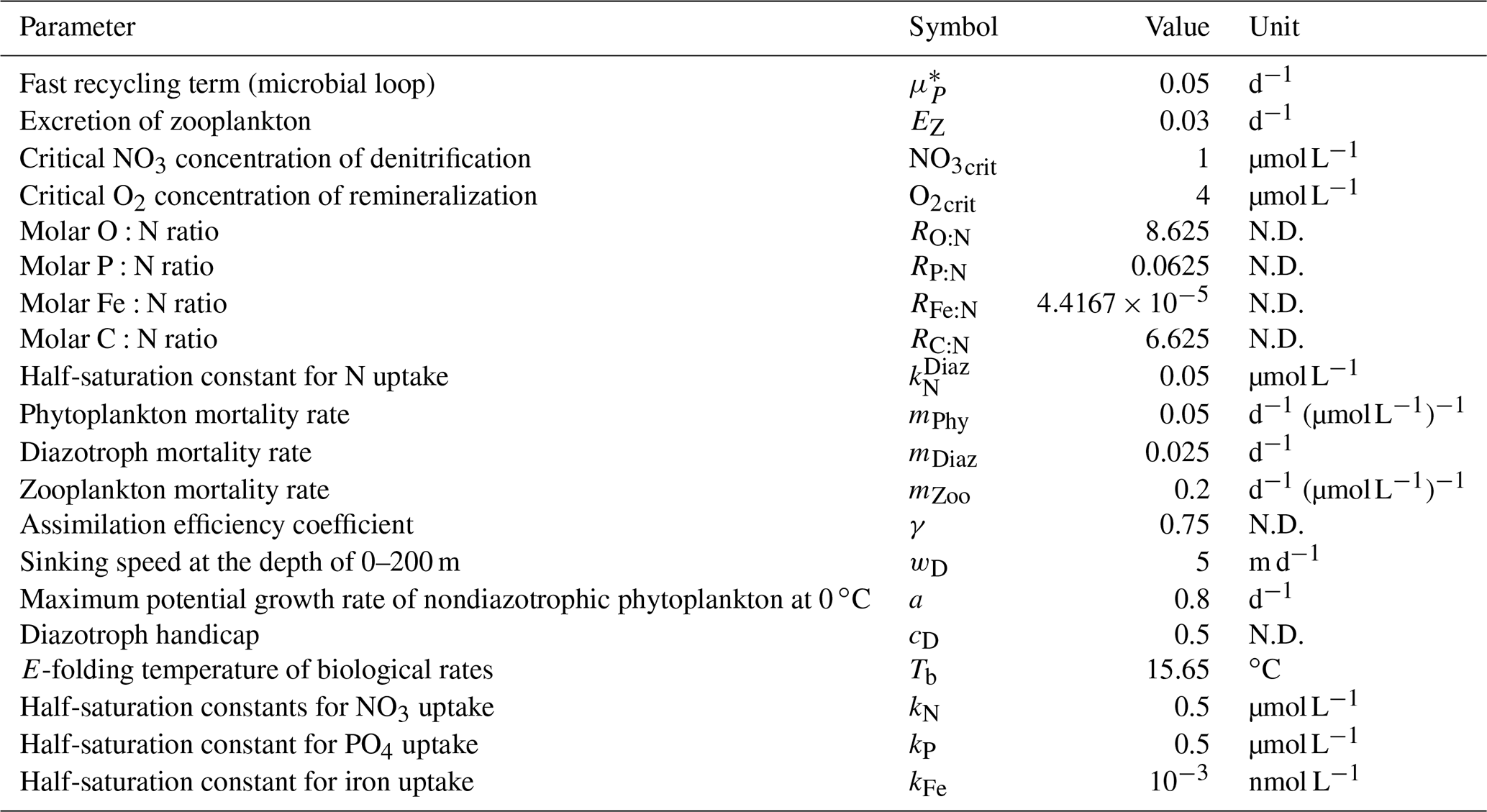
Table B2 Definitions of parameters and variables not mentioned specifically in the text.

Appendix C: Forcing data

The external forcing used for the HIST experiment is summarized in Table C1.

Table C1 List of forcing datasets for the HIST simulation: categories, variables, and references for the data creation and a description of how the datasets are applied in the HIST simulation in MIROC-ES2L.

Appendix D: Diagnosis of cumulative fossil fuel emission and atmospheric CO₂ concentration

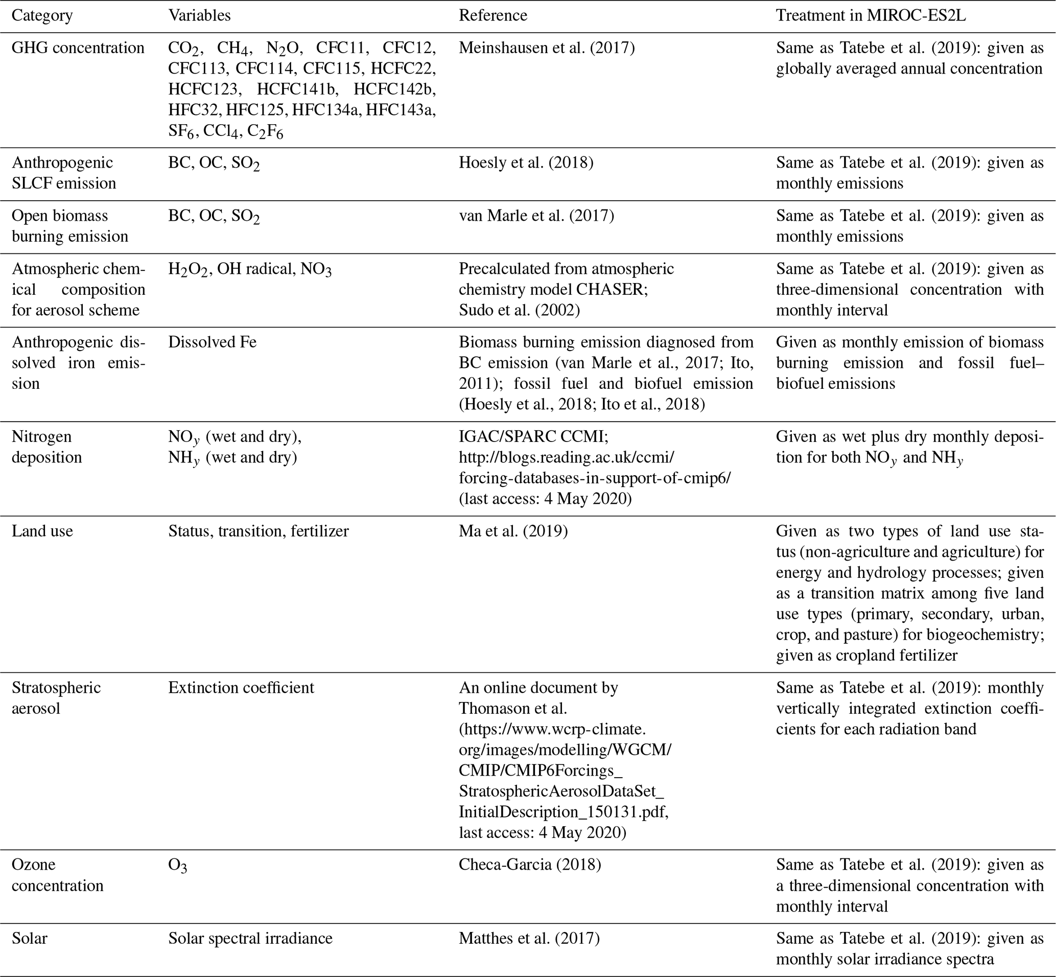
The global carbon budget can be written as follows:

$$\mathrm{CE}=\mathrm{CA}+\mathrm{CL}+\mathrm{CO},$$

where CE represents the cumulative emissions derived from fossil fuel and industry. CA, CL, and CO represent the changes in the carbon amount in the atmosphere, land, and ocean, respectively. When models are forced with a prescribed CO₂ concentration (CA), both CL and CO are diagnosed in the simulations. By expressing the prescribed CA as CA^P, the budget equation can be described as

$$\begin{array}{}\text{(D1)}& {\mathrm{CE}}^{\mathrm{D}}={\mathrm{CA}}^{\mathrm{P}}+\mathrm{CL}+\mathrm{CO},\end{array}$$

where CE^D is a diagnosed fossil fuel and industrial carbon emission, as analyzed in Jones et al. (2013).

If we can obtain the prescribed emission (CE^P) that is consistent with the historical atmospheric CO₂ concentration change, we can diagnose the CO₂ concentration (CA^D) as follows:

$$\begin{array}{}\text{(D2)}& {\mathrm{CA}}^{\mathrm{D}}={\mathrm{CE}}^{\mathrm{P}}-\mathrm{CL}-\mathrm{CO}.\end{array}$$

For CMIP6, CE^P during 1850–2014 was approximately 403 PgC, and the values of CL and CO in this study were 44 and 163 PgC, respectively. Thus, CA^D in this study was 193 PgC. This is equivalent to the CO₂ concentration change of 91 ppmv determined using a conversion factor of 2.12 (PgC ppmv⁻¹). Consequently, we can obtain the diagnosed CO₂ concentration at the end of the simulation (2014), i.e., 376 ppmv. We note that the estimate of anthropogenic CO₂ emissions from fossil fuel and industry has an uncertainty range. Le Quéré et al. (2018) estimate the cumulative emissions as 400±20 PgC for 1850–2014; however, this was not considered in this study. Additionally, there is a budget imbalance of 25 PgC in Le Quéré et al. (2018), which was also ignored in this study.

Appendix E: Feedback parameters of carbon cycle with same unit

As in Appendix D, the global carbon budget can be written as follows:

$$\begin{array}{}\text{(E1)}& \mathrm{CE}=\mathrm{CA}+\mathrm{CL}+\mathrm{CO}.\end{array}$$

Following Gregory et al. (2009), this carbon budget equation can relate the feedback parameters of land and ocean to AF. First, following the definition, CL and CO can be expressed by the feedback parameters of CO₂–carbon and climate–carbon feedbacks (β and γ, respectively) as follows:

$$\begin{array}{}\text{(E2)}& {\displaystyle }& {\displaystyle }\mathrm{CL}={\mathit{\beta }}_{\mathrm{L}}\mathrm{CA}+{\mathit{\gamma }}_{\mathrm{L}}T,\text{(E3)}& {\displaystyle }& {\displaystyle }\mathrm{CO}={\mathit{\beta }}_{\mathrm{O}}\mathrm{CA}+{\mathit{\gamma }}_{\mathrm{O}}T,\end{array}$$

where CA is the carbon increase in the atmosphere and T is global temperature change (T). Using Eqs. (E1)–(E3), the global carbon budget equation can be written as follows:

$$\begin{array}{}\text{(E4)}& \mathrm{CE}=\mathrm{CA}+\mathrm{CA}({\mathit{\beta }}_{\mathrm{L}}+{\mathit{\beta }}_{\mathrm{O}})+T({\mathit{\gamma }}_{\mathrm{L}}+{\mathit{\gamma }}_{\mathrm{O}}).\end{array}$$

Dividing both sides of the equation by CA leads to the following:

$$\begin{array}{}\text{(E5)}& \mathrm{CE}/\mathrm{CA}=\mathrm{1}+({\mathit{\beta }}_{\mathrm{L}}+{\mathit{\beta }}_{\mathrm{O}})+T({\mathit{\gamma }}_{\mathrm{L}}+{\mathit{\gamma }}_{\mathrm{O}})/\mathrm{CA}.\end{array}$$

Then, we define T∕CA =α, as used by Friedlingstein et al. (2006) or Arora et al. (2013), and we replace CE∕CA by 1∕AF (because AF = CA∕CE):

$$\begin{array}{}\text{(E6)}& \mathrm{1}/\mathrm{AF}=\mathrm{1}+({\mathit{\beta }}_{\mathrm{L}}+{\mathit{\beta }}_{\mathrm{O}})+\mathit{\alpha }({\mathit{\gamma }}_{\mathrm{L}}+{\mathit{\gamma }}_{\mathrm{O}}).\end{array}$$

The u quantity proposed by Gregory et al. (2009) is u_βL=β_L, u_βO=β_O, u_γL=αγ_L, and u_γO=αγ_O. Through replacement with the u terms, Eq. (E6) can be expressed as

$$\begin{array}{}\text{(E7)}& \mathrm{1}/\mathrm{AF}=\mathrm{1}+u_{\mathit{\beta }\mathrm{L}}+u_{\mathit{\beta }\mathrm{O}}+u_{\mathit{\gamma }\mathrm{L}}+u_{\mathit{\gamma }\mathrm{O}},\end{array}$$

and thus we obtain the following:

$$\begin{array}{}\text{(E8)}& \mathrm{AF}=\mathrm{1}/(\mathrm{1}+u_{\mathit{\beta }\mathrm{L}}+u_{\mathit{\beta }\mathrm{O}}+u_{\mathit{\gamma }\mathrm{L}}+u_{\mathit{\gamma }\mathrm{O}}).\end{array}$$

The unit of the u parameters is also dimensionless (AF unit: PgC PgC⁻¹).