the Creative Commons Attribution 4.0 License.
the Creative Commons Attribution 4.0 License.
 | 25 Mar 2020
PM2.5 ∕ PM10 ratio prediction based on a long short-term memory neural network in Wuhan, China
Xueling Wu
Ying Wang
Siyuan He
Zhongfang Wu
Air pollution is a serious problem in China that urgently needs to be addressed. Air pollution has a great impact on the lives of citizens and on urban development. The particulate matter (PM) value is usually used to indicate the degree of air pollution. In addition to that of PM2.5 and PM10, the use of the PM2.5 ∕ PM10 ratio as an indicator and assessor of air pollution has also become more widespread. This ratio reflects the air pollution conditions and pollution sources. In this paper, a better composite prediction system aimed at improving the accuracy and spatiotemporal applicability of PM2.5 ∕ PM10 was proposed. First, the aerosol optical depth (AOD) in 2017 in Wuhan was obtained based on Moderate Resolution Imaging Spectroradiometer (MODIS) images, with a 1 km spatial resolution, by using the dense dark vegetation (DDV) method. Second, the AOD was corrected by calculating the planetary boundary layer height (PBLH) and relative humidity (RH). Third, the coefficient of determination of the optimal subset selection was used to select the factor with the highest correlation with PM2.5 ∕ PM10 from meteorological factors and gaseous pollutants. Then, PM2.5 ∕ PM10 predictions based on time, space, and random patterns were obtained by using nine factors (the corrected AOD, meteorological data, and gaseous pollutant data) with the long short-term memory (LSTM) neural network method, which is a dynamic model that remembers historical information and applies it to the current output. Finally, the LSTM model prediction results were compared and analyzed with the results of other intelligent models. The results showed that the LSTM model had significant advantages in the average, maximum, and minimum accuracy and the stability of PM2.5 ∕ PM10 prediction.
- Article
(3864 KB) - Full-text XML
- BibTeX
- EndNote


Aerosol is a general term for solid and gas particles suspended in air. Aerosols can have an important impact on regional and global atmospheric environments, climates, and ecosystems and have long been an important issue in global environmental change research (Crutzen and Andreae, 1990). Particulate matter (PM) is usually separated and categorized based on its aerodynamic diameter, and the most widely monitored particles are PM10 and PM2.5. Particles with an aerodynamic particle size not exceeding 10 µm are called PM10. PM10 is primarily produced by industrial production, agricultural production, construction, roadside dust, various industrial processes, and natural processes such as the resuspension of local soil and dust storms. Particles with an aerodynamic particle size not exceeding 2.5 µm are called fine PM (PM2.5) and are mainly derived from anthropogenic emissions. PM2.5 is mainly produced by anthropogenic combustion for transportation and energy production, and it is particularly important in environmental policy and public health (Xie et al., 2011). Infectious disease research shows that there is a significant consistency between the PM2.5 environmental quality concentration and adverse effects on human health (Lelieveld et al., 2015). PM2.5 mainly causes damage to the respiratory and cardiovascular systems, including coughing, difficulty breathing, lowered lung function, and aggravated asthma, causing chronic bronchitis, arrhythmia, nonfatal heart disease, and premature death of patients with cardiopulmonary disease (Wu et al., 2011; Jia et al., 2012). In addition, since the scattering extinction contribution of PM2.5 particles accounts for 80 % of the extinction of the atmosphere, the concentration of PM2.5 is a key factor in determining the visibility of the atmosphere (Sisler and Malm, 1997). In view of the importance of aerosols and near-surface atmospheric PM2.5 to regional and global climates and environments, quantitative and accurate observations using a variety of observation methods have become a hot research topic domestically and internationally (Dominici et al., 2006). Since fine and coarse particles come from different sources, the PM2.5–PM10-scale model has different physicochemical properties, which can not only distinguish the type of aerosol in the PM but also provide the mixing ratio of dust and artificial aerosols (Sugimoto et al., 2015). The PM2.5–PM10 scale is the main indicator for macro analysis of the source of particulate pollution in a region, which is more practical than considering PM2.5 and PM10 separately. For the research conducted in an urban area of northwestern China, PM10 and PM2.5 concentration data were collected to reveal the spatiotemporal behavior of local PM and mineral dust fractions (Qingyu et al., 2018).
The aerosol optical depth (AOD) is defined as the integral of the extinction coefficient of a medium in the vertical direction, which describes the effect of aerosols on light reduction. A study conducted by Hidy in 2009 indicated that the estimation of the PM2.5 concentration near the ground by satellite remote sensing AOD has great research potential (Hidy, 2009). The advantage is that satellite remote sensing data are generally standardized data with high reliability and a wide spatial coverage, providing wide-area, spatially continuous, and real-time monitoring information for regional and global PM2.5 air quality assessment. There are many ways to obtain the AOD from satellite sensors such as the Geostationary Operational Environmental Satellites (GOES) (Prados et al., 2007), the Advanced Very High Resolution Radiometer (AVHRR) (Gao et al., 2016), and the Moderate Resolution Imaging Spectroradiometer (MODIS) (Levy et al., 2013). MODIS data are one of the most widely used data sources for deriving ground PM2.5 concentrations with AOD (Hu et al., 2014). There are many ways to obtain AOD through MODIS data. For example, Yang et al. used the data collected by Landsat 8 satellite images to retrieve the AOD in Beijing by means of the Dark Target method and the visible near-infrared atmospheric correction method. The accuracy was verified by the Aerosol Robotic Network (AERONET) observation data (Ou et al., 2017). The Dark Blue AOD retrieval method was used to complement the Dark Target results by retrieving the AOD over bright arid land surfaces, such as deserts (Sayer et al., 2013). In addition, a new method that considers bidirectional reflectance of the surface was proposed, which is suitable for calculating the AOD in arid or semiarid regions (Xinpeng et al., 2018).
Although the relationship between the AOD and PM has been proven by many scholars, since the PM concentration level is usually measured at the surface, the correlation between them is affected by the planetary boundary layer height (PBLH) and relative humidity (RH) (Stirnberg et al., 2018; Chen et al., 2017). When studying the seasonal PM10–AOD correlation in northern Italy, Arvani et al. (2016) found that the introduction of PBLH and RH correction can significantly improve the bin-averaged PM–AOD correlation. After the vertical and RH correction methods were applied to the air quality station in Beijing, the determination coefficient R2 of the AOD and PM10 increased by 0.13, and the correlation between the AOD and PM2.5 increased from 0.48 to 0.62 (Wang et al., 2010). These calibration methods usually require the use of meteorological data to perform the calculations, and the addition of meteorological data to the evaluation of PM concentration can provide more reliable results. For instance, Jung et al. (2017) joined meteorological data to obtain an improved model of the surface PM2.5 from 2005 to 2015 to estimate the PM concentration for the entire main island of Taiwan.
Many statistical models have been used for the ground PM estimation of AOD and other predictors, such as linear regression models (Kim et al., 2019), random forest models (Stafoggia et al., 2019), neural network models (Sowden et al., 2018), and generalized additive models (Chen et al., 2018). However, with the introduction of new machine learning models, the traditional regression model reflects the inability to balance time, space, and random precision. The time precision mentioned in this article refers to the accuracy of inputting time-series data to predict the subsequent period results; the spatial precision refers to the accuracy of inputting all-time data of spatial points to predict the result of another spatial point; the random accuracy refers to the accuracy of inputting data of any time and space to predict the random selection data. One way to overcome these limitations is the long short-term memory (LSTM) model. The LSTM network is ideal for learning from experience so that time series can be classified, processed, and predicted with very long unknown time lags between important events. In the study of PM2.5 monitoring and prediction in smart cities, Chiou-Jye and Ping-Huan (2018) proposed that the prediction accuracy of the convolutional neural network (CNN)-LSTM model is the highest compared to the prediction accuracies of several other classic machine learning methods.
At present, air quality monitoring is still mainly based on monitoring stations, and it is difficult to acquire large-scale and accurate prediction results. In order to reduce the dependence on monitoring stations and achieve the goal of broad, rapid, and accurate air quality predictions, this paper aims to use a machine learning algorithm, combined with AOD and gaseous pollutant and meteorological data, to obtain a spatially and temporally reliable prediction model. This paper used a total of 59 AOD results for all of 2017 by the dense dark vegetation (DDV) method using MODIS level-2 data of Wuhan with a spatial resolution of 1 km. Since there were only 10 air quality stations in Wuhan, to ensure accuracy, the AOD values were extracted at the air quality station site, and the integration of the AOD, air pollutants, and meteorological data was also based on the station site. AOD* was obtained by correcting AOD using the PBLH and RH. Then, the R2-based optimal subset selection method was used to select the most relevant factor for PM2.5 ∕ PM10 from the meteorological factors and air pollutants. Finally, the space and timescales and random PM2.5 ∕ PM10 predictions were determined and performed, respectively, via the LSTM model, and the prediction results of the LSTM model and other classical models were compared and analyzed. The results showed that the average error of the LSTM model prediction results is very low, both spatially and temporally, and the stability of the prediction model is significantly better than that of other models.
Wuhan is the provincial capital of Hubei Province. The administrative extent is between 113.683 and 115.083∘ E and 29.967 and 31.367∘ N, and the total area is 8494.41 km2 (Zhou and Chen, 2018). The largest distance is between the eastern and western parts of Wuhan and is 134 km, and the maximum distance from north to south is 155 km. Wuhan is the city with the largest population, is the largest provincial capital city, has the most complicated road traffic, and has the most developed economy in the central part of the country (Jiao et al., 2017). The Yangtze River flows through Wuhan, and there are hundreds of lakes in Wuhan. The terrain of Wuhan is mainly plains, with low levels in the middle of the region and low mountains, hills, and ridges to the south and north. The climate type is a humid, north subtropical monsoon climate with high temperatures in summer, low temperatures in winter, and an annual average temperature of 15.9 ∘C. Sunshine hours and total radiation are also at high levels, and the annual average precipitation is approximately 1300 mm. June and August receive the most precipitation in Wuhan, and summer precipitation accounts for approximately 40 % of the annual rainfall. In recent years, the air quality in Wuhan has been improved. In 2017, the number of days in which the annual air quality level was acceptable was 255 d, and the acceptability rate was 69.9 %. At the same time, the number of days with light pollution, moderate pollution, heavy pollution, and severe pollution were 86, 17, 6, and 1 d, respectively.
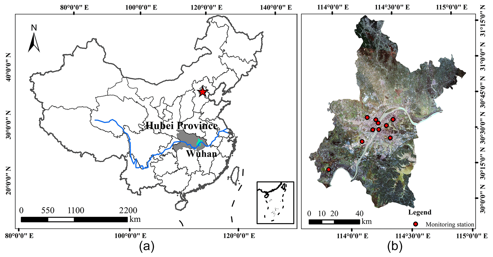
Figure 1Location of the study area in China (a: map of China; b: map of Wuhan area using bands 4, 3, and 2 of Landsat 8 OLI (Operational Land Imager) image).
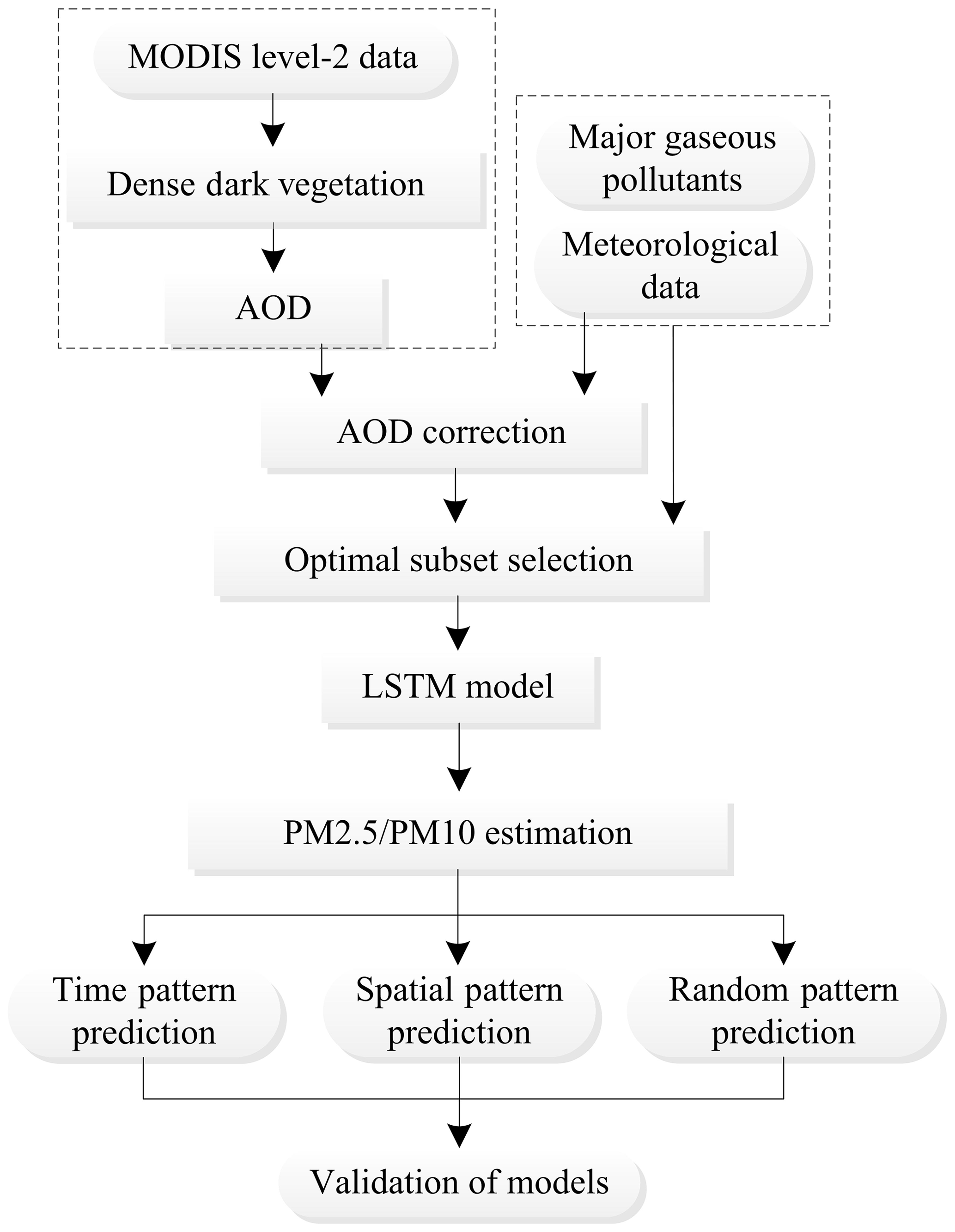
The data that our environmental monitoring station can monitor is only real-time data with no predicting of subsequent data in advance. If we want to predict the state of the air afterwards, we can use other relevant factors for reference. The AOD, which has a great relationship with PM, is an important parameter in the study of atmospheric aerosols. Gaseous pollutants are also a key factor in air quality. In addition, changes in meteorological conditions have an impact on PM. Therefore, we used the true air quality data from the ground monitoring stations as the inspection standard for verification and extracted the values of PM2.5, PM10, and gaseous pollutant with the data from the monitoring stations. After retrieving the AOD with the MODIS images five times a month, on average, in 2017, the AOD values at the monitoring stations were extracted, and the values of the meteorological data were also interpolated at the same point. Then, the AOD was corrected to obtain the AOD*, and gaseous pollutant data at the monitoring stations were added. The best set that predicted air quality was selected, and machine learning techniques were used to obtain models that can make space and time series predictions (Fig. 2).
3.1 AOD retrieval
MODIS is an important sensor on the Terra and Aqua satellites. The Terra satellite passes from north to south at approximately 10:30 LT, and Aqua moves from south to north at 13:30 LT. Wuhan is located in the central and eastern parts of Hubei Province at the southeast corner of the h27v05 frame; therefore, we chose to use the images collected by Terra because of its higher image quality. The MODIS data have 36 spectral bands, ranging from 0.4 to 14.4 µm, of which seven bands can be used to retrieve the AOD, while the best bands for over-land aerosol retrieval are 0.47, 0.66, and 2.12 µm, especially in areas with dense vegetation. We downloaded the MOD02_L1B data for the region in Wuhan in 2017 via the website (https://ladsweb.modaps.eosdis.nasa.gov, last access: 8 June 2018) and removed a number of days with a large amount of clouds, finally obtaining 59 images with a spatial resolution of 1 km. According to the DDV method (Li et al., 2014), after radiation correction, geometric correction, angle data resampling, and angle data geometric correction and synthesis, cloud detection processing was performed; then, a lookup table file was generated according to the “6S” (second simulation of the satellite signal in the solar spectrum) atmospheric radiation model, and the AOD was acquired (Fig. 3). After verifying with the MOD04_L2 aerosol product data released by the National Aeronautics and Space Administration (NASA), the results of the retrieval were considered valid and used later. Figure 4 shows the results of the AOD retrieval on 18 July.
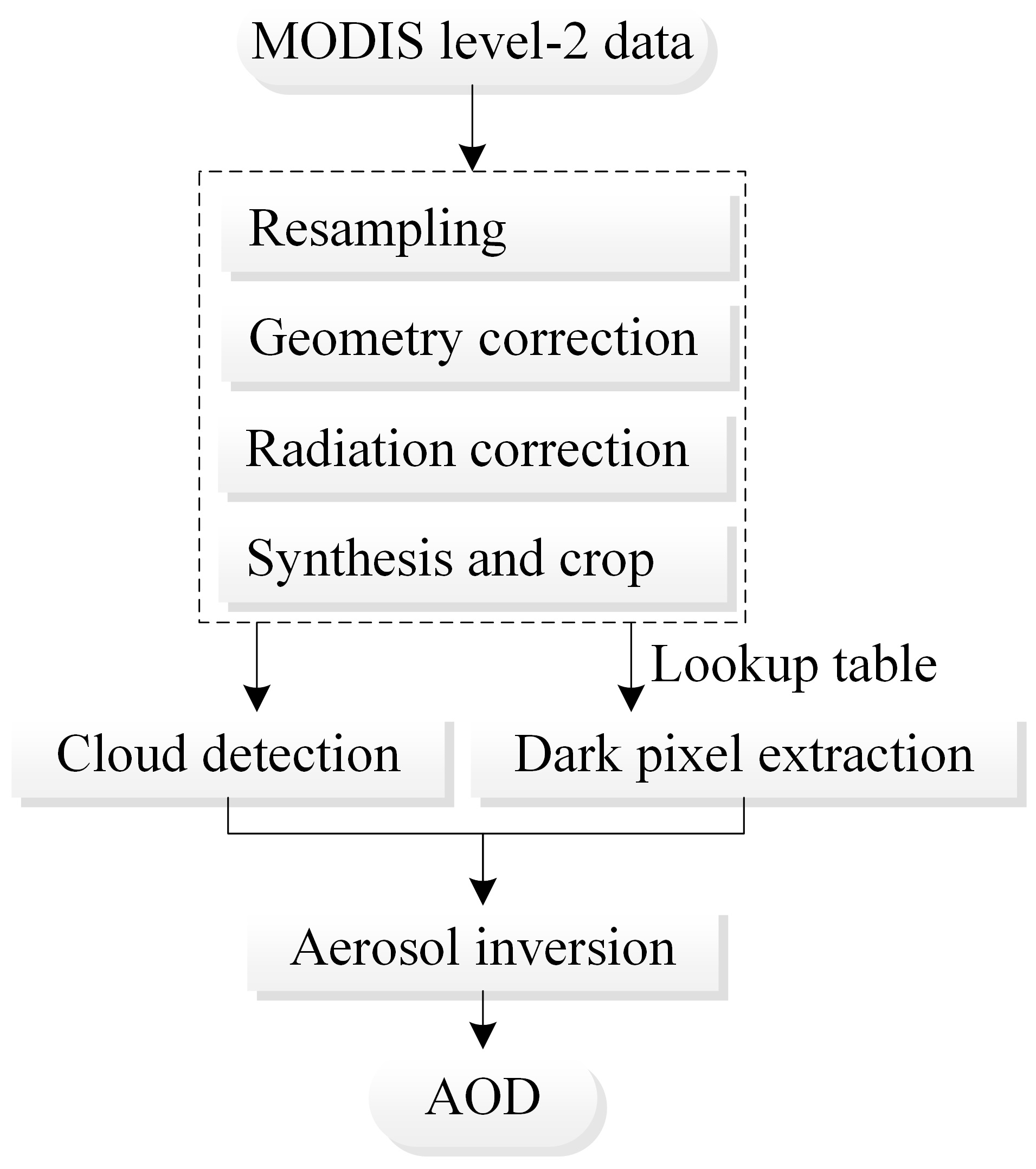

Figure 4AOD retrieval on 18 July.
3.2 Ground-level air quality and gaseous pollutant data
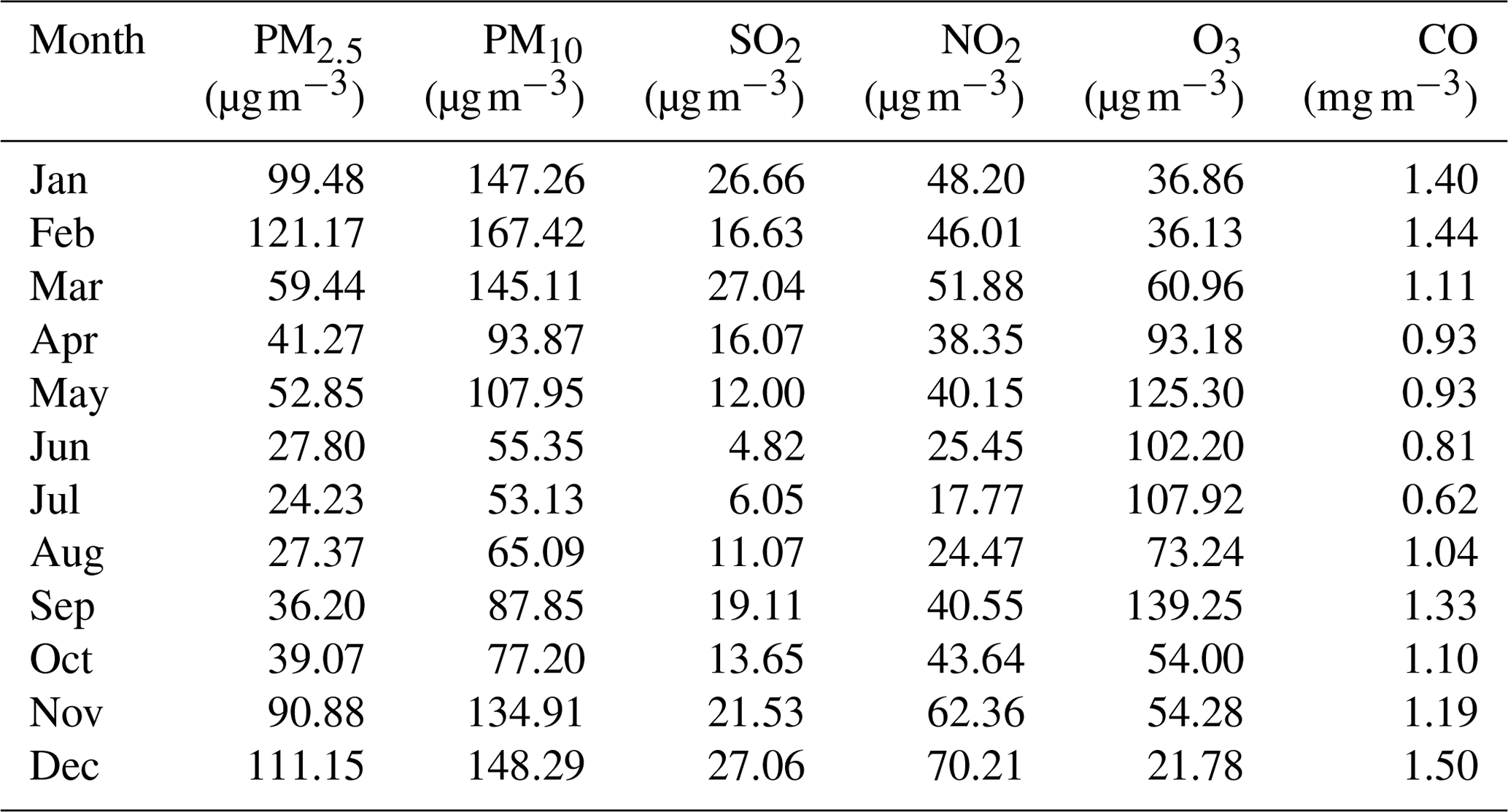
The Ministry of Ecology and Environment of China has established 10 national environmental quality control stations in Wuhan. The shortest distance between points is more than 3 km, and the average distance is about 10 km. Each station continuously collects hourly average concentration values of PM2.5, PM10, SO2, NO2, O3, and CO and publishes the daily average concentration values. The calculations in this paper were based on these daily averaged data, which were released by the China National Environmental Monitoring Center (http://webinterface.cnemc.cn/cskqzlrbxsb2092932.jhtml, last access: 14 May 2018). The monthly average concentration data of PM2.5, PM10, and gaseous pollutants obtained from these data in 2017 are shown in Table 1. During the year, the trends in PM2.5 and PM10 were roughly the same. The maximum values of PM2.5 and PM10 reached 121.17 and 167.42 µg m−3, respectively, in February. From February to July, the values dropped rapidly, reaching minimum levels in July of 24.23 and 53.13 µg m−3, respectively. After July, the concentration of PM2.5 continued to rise, and the growth rate accelerated. The concentration of PM10 also increased after July but decreased between September and October. NO2 is mainly derived from the high-temperature combustion process of fossil fuels. The combustion of nitrogen-containing fuels (such as coal) and nitrogen-containing chemicals can directly release NO2. In general, motor vehicle emissions are one of the main sources of urban NO2. SO2 is a ubiquitous pollutant in cities. The SO2 in the air mainly comes from the industrial production of thermal power generation and other industries, such as the following: the combustion of fixed-source fuels; the production of nonferrous metals; the production of steel, chemical, and sulfur plants; and discharge from small heating boilers and civil coal furnaces. Natural processes, such as volcanic activity, also emit a certain amount of SO2. CO is a colorless, odorless, flammable, and toxic gas that is a product of the incomplete combustion of carbonaceous fuels. The concentrations of SO2, NO2, and CO showed regularity. The concentration in summer was the lowest, followed by spring and autumn, and the highest was in winter. The lowest value was in June or July, and the highest was in December. O3 is a representative pollutant for photochemical smog, which is formed and enriched by nitrogen oxides and hydrocarbons in the air under intense sunlight and through a series of complex atmospheric chemical reactions. Although O3 in the upper stratosphere has important anti-radiation protection for life on Earth, O3 at low altitudes in cities is a very harmful pollutant. The trend in the O3 concentration was different, where the winter value was low and then increased in spring with time. In summer, the O3 concentration fluctuated at a higher level and decreased in autumn.
Table 1Monthly average concentrations of PM2.5, PM10, and gaseous pollutants in Wuhan in 2017.
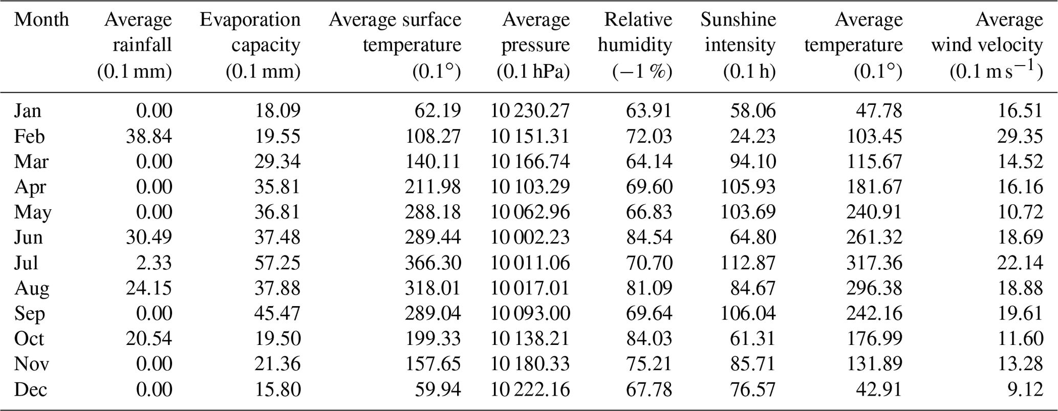
3.3 Meteorological data
The quality of air is closely related to meteorological conditions. The meteorological data obtained in this paper derive from the National Meteorological Information Center of China's National Meteorological Information Network (http://data.cma.cn/site/index.html, last access: 9 October 2018) and include average rainfall, evaporation capacity, RH, sunshine intensity, average surface temperature, average wind velocity, average air pressure, and average temperature. The data obtained were daily average data in 2017. A total of five meteorological stations exist near the Wuhan area. To obtain meteorological data near the air quality monitoring stations, data from the meteorological stations needed to be interpolated. We believe that the kriging method is the most appropriate for examining the spatial characteristics of meteorological data. The kriging method is a multistep process that includes exploratory statistical analysis of the data, variogram modeling, surface creation, and studying the various surfaces. The kriging method interpolates unknown samples according to the distribution characteristics of a few well-known data points in a finite neighborhood. After taking into account the size, shape, and spatial orientation of the sample points, combining the spatial relationship between the known sample points and the unknown samples, and adding the structural information provided by the variogram, kriging performs a linear unbiased optimal estimation of the unknown samples in the spatial range. After comparing the kriging, natural neighbor, spline, and inverse distance weighted methods, we found that the results acquired by setting 12 interpolation points and using the spherical model of the kriging method were smoother and more suitable for the study area. The monthly averages of the meteorological data at all of the calculated sites are shown in Table 2. The seasonal changes reflected by several meteorological data results were more obvious. The average surface temperature and average temperature were higher in summer and lower in winter. The average air pressure had a completely opposite trend. The sunshine intensity and evaporation capacity were lower in winter and fluctuated in the other three quarters. The rainfall was concentrated in summer and autumn, while the average wind velocity and RH had no obvious seasonal characteristics.
4.1 AOD correction
The PBLH refers to the thickness of the planetary boundary layer and is an important physical parameter for numerical atmospheric models and environmental evaluations (Su et al., 2018). The PBLH is calculated by a commonly used national standard method in China. The national standard method is performed according to the method specified in the Chinese national standard GB/T13201-91 (http://www.mee.gov.cn/gzfw_13107/kjbz/qthjbhbz/qt/201605/t20160522 342349.shtml, last access: 14 December 2019). This method assumes that the thermal conditions of the near-surface layer depend, to a large extent, on the degree of ground heating and cooling. This method takes into account the thermal and dynamic factors and quantifies the solar elevation angle, cloud volume, and wind speed. Then, according to the specified local parameters, the atmospheric stability is classified into A, B, C, and D categories according to the Pasquill stability classification:
When the atmospheric stability is E and F,
where h (in meters) is the thickness of the mixing layer; U10 (in meters per second) is the average wind velocity at a height of 10 m, which is 6 m s−1; as and bs are the mixing layer coefficients; f is the ground rotation parameter; Ω is the ground rotation angular velocity, with a value of rad s−1; and φ (in degrees) is the geographic latitude.
The aerosol hygroscopic growth factor f(RH), where RH is the relative humidity, describes the extent to which the aerosol extinction cross section or scattering coefficient increases with increasing RH, depending on a variety of factors, such as the temperature absorption properties of the aerosol (Cai et al., 2018). The common formula for calculating f(RH) is
Since the parameters describing atmospheric physical conditions, such as air pressure, atmospheric temperature and atmospheric humidity change, existing much more in the vertical than horizontal direction, it is often assumed that the atmosphere has a structure in which the horizontal direction is uniform and the vertical direction is layered. For the single homogeneous distribution of spherical aerosol particles, the near-surface particle concentration can be obtained by measuring a dry air sample. The expression is as follows:
where ρ (in grams per cubic meter) is the average density of the particles and n(r) is the particle spectral distribution function under ambient humidity, which is related to the particle size.
Given the wavelength of the radiation, the aerosol optical thickness from the ground to a height of H can be expressed as
To convert Qext,amb under ambient humidity to Qext,dry under dry conditions, a hygroscopic growth factor f(RH) is required. This factor represents the ratio of normalized particle scattering efficiency under ambient RH and dry conditions and is a function of humidity:
A normalized particle scattering efficiency Qext and a parameterized expression of the effective radius reff are introduced for replacement in the above formula:
Finally, the relationship between the AOD and near-surface PM2.5 mass concentration is introduced as follows:
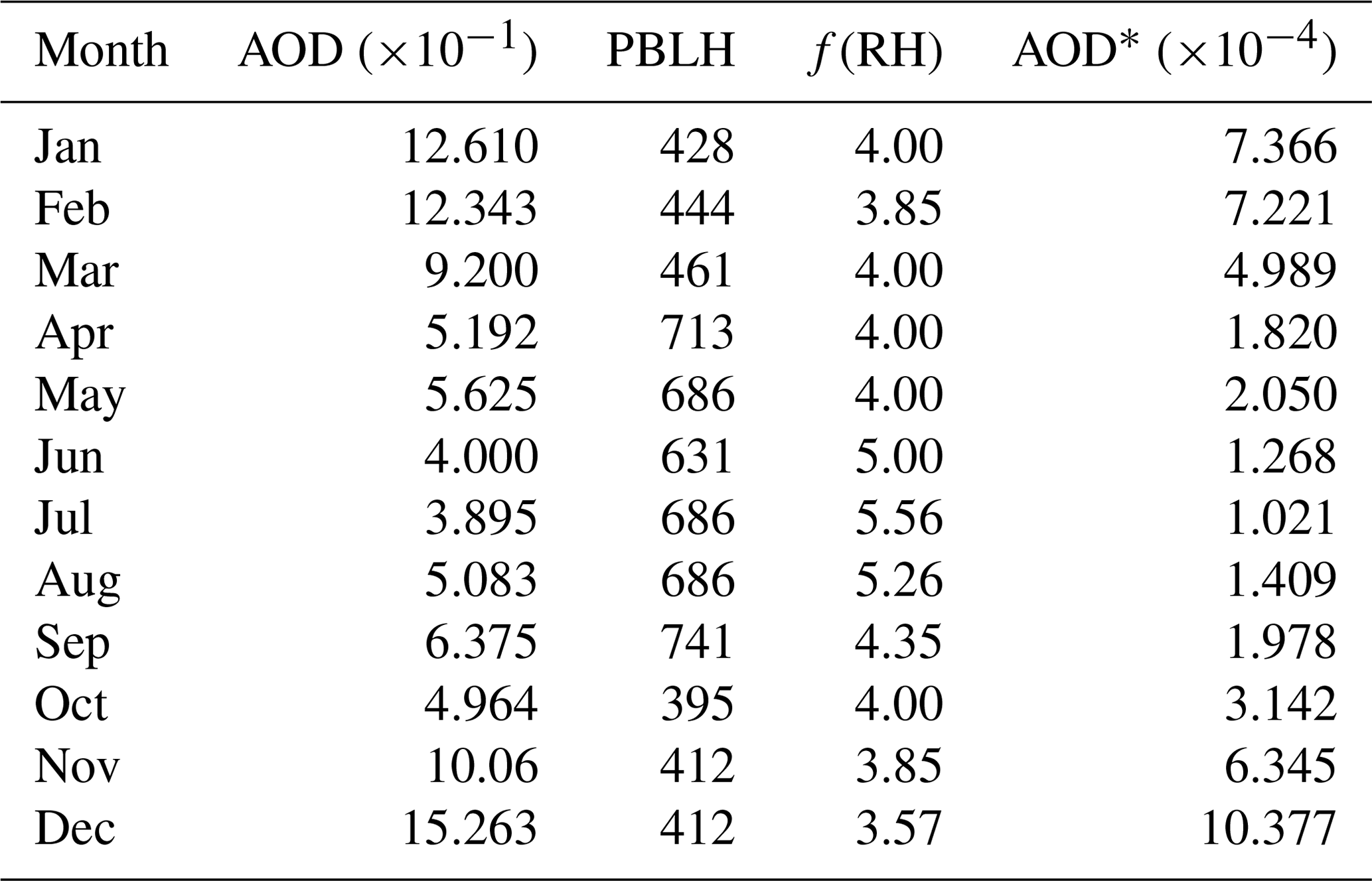
where S (in square meters per gram) represents the specific extinction efficiency of the aerosol under ambient humidity conditions. H stands for aerosol elevation. In practice, the PBLH approximation is often used instead of H. According to the above relationship between the AOD and PM2.5, it can be inferred that if the AOD is corrected by the factors PBLH and f(RH), the corrected AOD*, that is, AOD∕(PBLH ×f(RH)), is expected to have better correlation with PM. Taking the monthly average value as an example, the parameters PBLH and f(RH) used by the AOD correction algorithm, and the corrected AOD* are shown in Table 3. The monthly average data of PM2.5 ∕ PM10, AOD, and AOD* are shown in Fig. 5. In fact, after calculating the linear correlations of the AOD and AOD* with PM2.5 ∕ PM10, the correlation increased from 0.838 to 0.873.

4.2 Selection factors
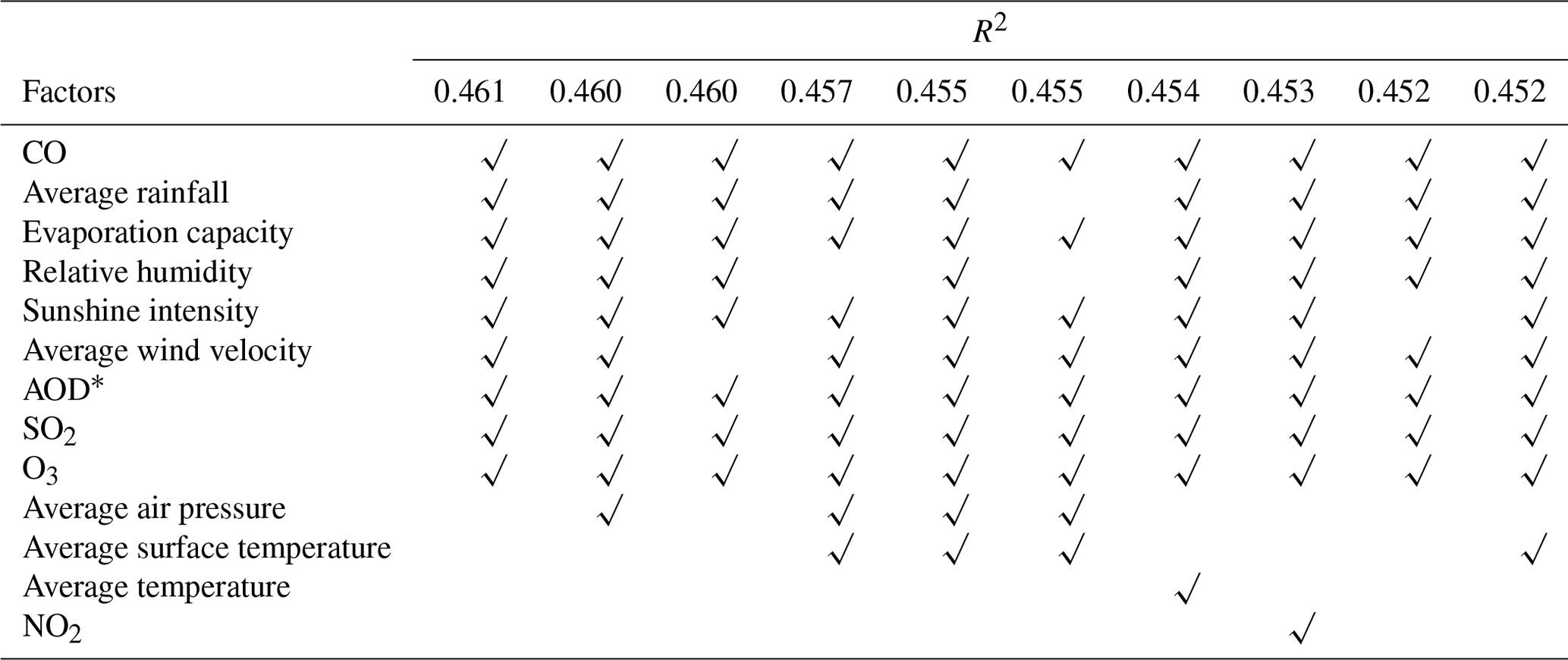
When choosing a subset, the choice of independent variables should be practical. How to choose the best subset of variables in order to establish a better regression equation has been a hot research topic. The process of the optimal subset method is as follows: first, in a set containing multiple independent variables, freely selecting and combining from each independent variable; next, combining all independent variables and dependent variables to establish all possible equations; and then the best independent variable combination model is selected from all of the fitted regression equations. The optimal subset method can determine an optimal regression equation from all possible subsets via some criteria and has been widely used in weather and climate predictions. Using the correlation coefficient R2 as the evaluation index and the optimal subset of PM2.5 ∕ PM10 as the dependent variable, the highest R2 is 0.461. The independent variables in the subset are as follows: AOD*; average rainfall; evaporation capacity; RH; sunshine intensity; average wind velocity; and SO2, CO, and O3 concentrations. The factors selected by the optimal subset method are shown in Table 4. This table shows the top 10 scores for R2 scores and the corresponding factor combinations. The symbol “√” indicates that the factor is selected.
4.3 RNNs and the LSTM model
The recurrent neural network (RNN) is a powerful deep neural network that uses its internal memory to process input sequences with any timing. In the RNN model, compared with the common multilayer neural network, the interconnection layer is added between the nodes of the hidden layer, and the directional loop is formed by the connection between the hidden layer neural units; then, the internal state of the network is created, and the dynamic time series behavior is presented (Bao and Zeng, 2013). The RNN can handle any sequence length in principle, but in an actual situation, the standard RNN model cannot store sequence information about the past and lacks the ability to establish remote structure connections. This kind of “forgetting” limitation cannot record long-term information. Thus, these networks are more prone to instability when generating sequences, resulting in a time dependency problem. This problem is not unique to RNNs but exists in almost all generation models. The LSTM model is a network that is used to address long-term time-dependent dependencies. It is a time RNN suitable for processing and predicting important events with relatively long intervals and delays in time series (Weninger et al., 2014, 2015; Pei et al., 2015).
The key to distinguishing the LSTM model from the traditional RNN is that the traditional RNN has only one hidden layer output value state h, and h changes with the convolution process and is insensitive to long-term or long-distance events. The LSTM model adds a cell state c to store the long-term status. The calculation process after adding c is shown in Fig. 6, where x, h, and c are vectors. At time t, there are three inputs to the LSTM: the input value xt of the current time network, the output value ht−1 of the LSTM model at the previous time, and the cell state ct−1 of the previous time. The two outputs of the LSTM are the current time LSTM output value ht and the current state of the unit ct.

Figure 6 emphasizes the calculation process of the cell state c, and the overall process of the LSTM model is shown in Fig. 7. The key point of the LSTM model is how to control the state c. The idea of the LSTM model is to use three control switches to control it. The switches implemented in the algorithm are known as “gates”, which are fully connected layers whose input is a vector, and the output is a real vector between 0 and 1 (Srivastava and Lessmann, 2018). The input gate determines how much of the input xt of the network is saved to the cell state ct at the current moment, the forget gate determines how much the cell state ct−1 at the previous moment is retained as the current moment ct, and the output gate controls how much the cell state ct is output to the current output value ht of the LSTM. Assuming W is the weight vector of a gate and b is the bias value, then the gate can be expressed as:
These three gates are defined as follows:
where it, ft, and ot are the values of the input, forget, and output gates, respectively; σ is the activation function; and bi, bf, and bo are their respective bias values. The structure of the LSTM model is shown in Fig. 7. The inputs are in terms of time, space, and randomness, and the outputs are their results.
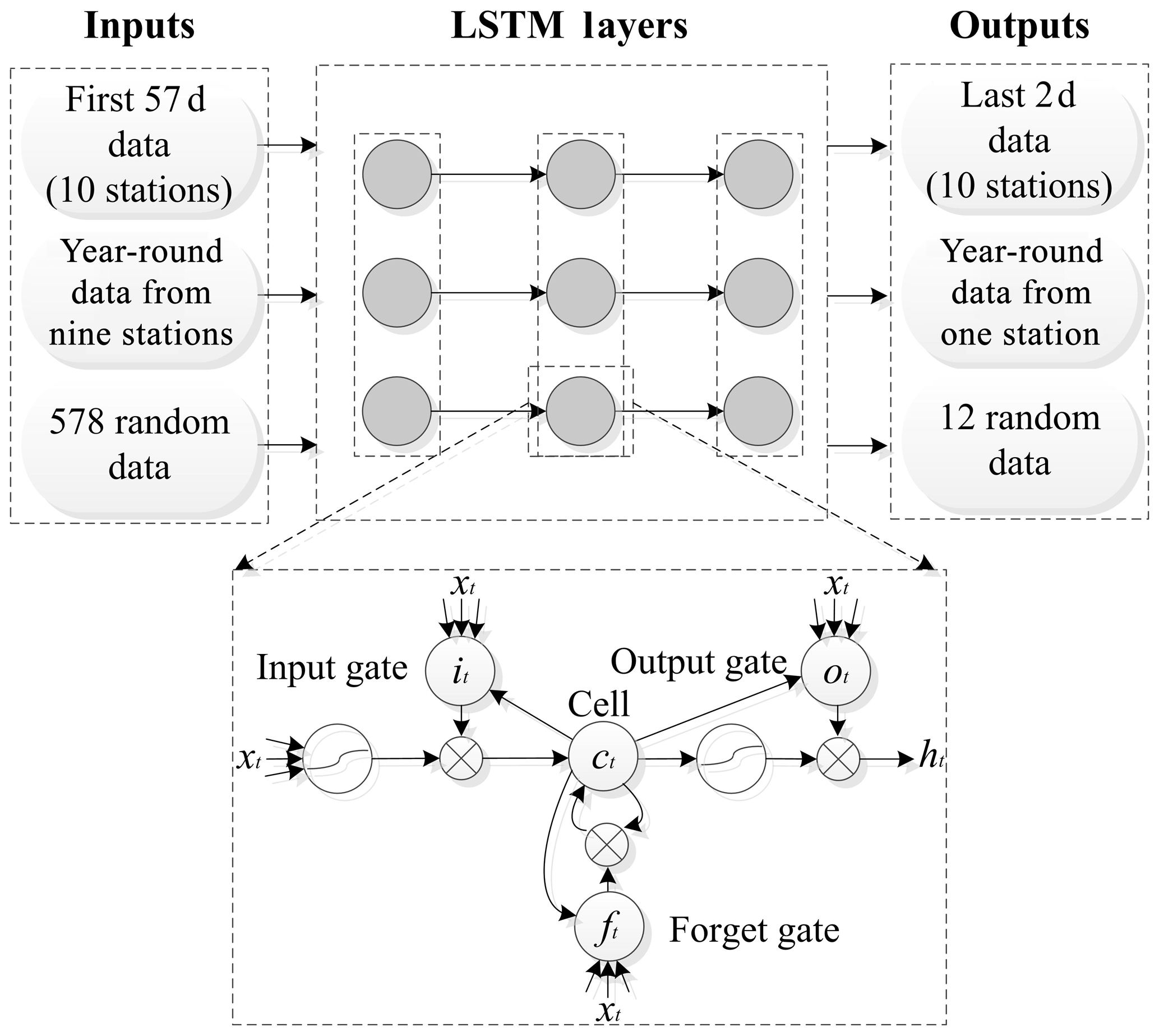
Time, space, and random prediction patterns can be used to judge the practicability of the prediction model from various perspectives. The time model took the first 57 data points from 2017 as input and predicted the last 2 d by applying the LSTM model. The spatial model used the data from the nine stations throughout the year as the input and obtained prediction results for the one remaining station. The random model randomly extracted 578 data for the input and the remaining 12 data for the verification. The error rate was obtained by comparing the prediction results with the actual values from monitoring. The implementation of the LSTM models is based on Keras, which is a high-level neural network application programming interface written in Python.
To determine the appropriate number of layers for the LSTM method, except for the data used for prediction, we divided the data set involved in the model construction into three parts: 40 % of the data were used as the training samples for modeling, 30 % of the data were used as the test samples, and the remaining 30 % of the data were used as verification data. We tried to use various LSTM architecture layers for the comparison. After obtaining the results of various LSTM architecture layers, we found that the results obtained using the LSTM architecture with four layers were the best, with the first three layers and the dense layer as the last layer. The role of the dense layer is to complete the final output of unique values. Because the LSTM uses the activation function as the gate, the outputs of the gates must be between 0 and 1, and the output ranges of both types of activation functions must be satisfied. We determined that the activation function for setting the forget gate and the input gate was defined as a sigmoid function. After adjusting the number of neurons, the number of epochs, and the batch size, the loss function we obtained has converged without overfitting.
5.1 Time pattern prediction
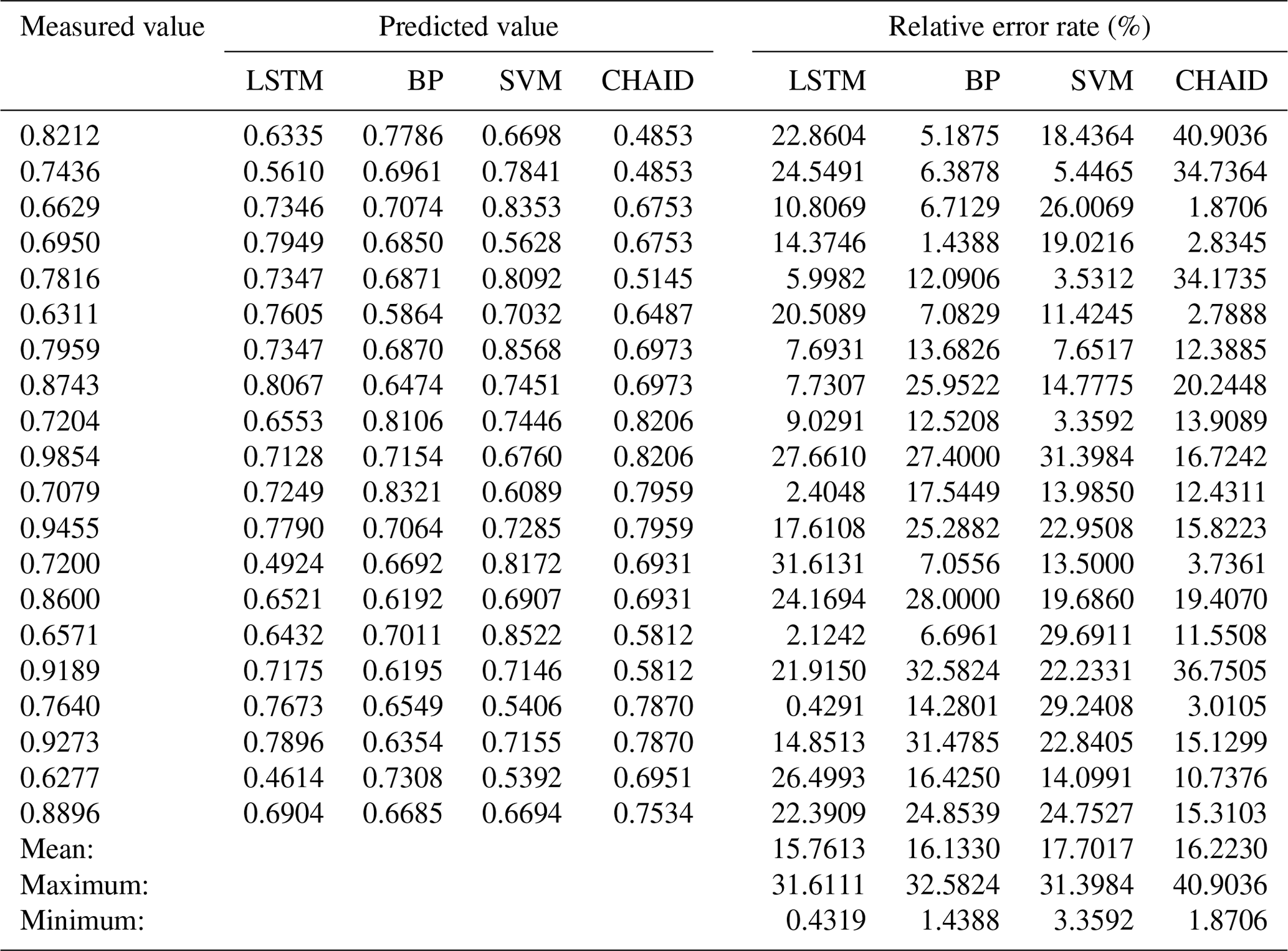
Using the input of the first 57 d in the 2017 data from 10 sites, there were 570 input samples, and the data used to verify the model were from the last 2 d in 2017. These 2 d were 25 and 31 December. In winter, with a high PM2.5 ∕ PM10 value, the ratios were more concentrated above 0.6. We compared the prediction results of the LSTM model with the back propagation (BP) neural network, support vector machine (SVM), and chi-squared automatic interaction detection (CHAID) decision tree models. Then, we calculated the error rate between the predicted value and the measured value (Table 5). Among the four algorithms, the average error of the LSTM model was the smallest, 15.7613, and its minimum error was also the smallest, only 0.4319, but its maximum error value was a little larger than SVM maximum errors values. The BP network method and the SVM had similar prediction results; the average error was not too large, and the maximum error value was small, while the minimum error value was larger. Although the average error of the CHAID model was small, the minimum error and the maximum error values were both bad. None of the four prediction methods could accurately predict the case where the PM2.5 ∕ PM10 value was greater than 0.9. The maximum value that the LSTM was able to predict was 0.8067. In air quality research, predictions of higher values are particularly important, because only a successful prediction of poor air quality can be used to promptly remind people to take preventive measures, such as wearing masks. This table was produced in site order, i.e., the first and second data entries are from the same site for the last 2 d of 2017, and the third and fourth data are from another site. The actual data for PM2.5 ∕ PM10 on the first day were generally lower than those on the next day, and the data from seven of the sites on the last day were larger than 0.8. Only the LSTM model can produce stable and higher predictions. In the other models, the average value of PM2.5 ∕ PM10 on the day when the air quality is bad is less than 0.7, while the average value of PM2.5 ∕ PM10 of the LSTM model is 0.726. This result indicates that LSTM produced better predictions at higher values than the other machine learning model algorithms.
Table 5The results and relative error rates of the time pattern predictions.
5.2 Spatial pattern prediction
One station was used as the output to be predicted; the other nine sites were inputs, and the prediction results of the spatial pattern were obtained. The output site is located in the southwest corner of Wuhan, which is the farthest from the other stations, and the distance from the nearest station is 34.7 km. Since the prediction site had no input data for the whole year and is far away from the other nine stations, the prediction result was less accurate than the time and random prediction results. However, this prediction method can better reflect the applicability of the model to spatial prediction. The relative error rates of the predicted results of the four models are shown in Table 6. The average error rate of the LSTM model was still the lowest, along with the maximum error value and minimum error rate, which was much smaller than that of the other models. In this spatial prediction, the accuracy of the prediction result when the PM2.5 ∕ PM10 ratio was lower than 0.2 was the lowest, and the accuracy of the prediction result when the PM2.5 ∕ PM10 ratio was larger than 0.8 was better than that when the PM2.5 ∕ PM10 ratio was lower than 0.2. The prediction results in other cases were much better. In addition, we also conducted experiments using one station located in the central area of Wuhan as the output. The results of the LSTM model showed that the prediction results at this point were much better than those at the southwest point, and the average error rate was 25.1664 %.
Table 6The results and relative error rates of the spatial pattern prediction.
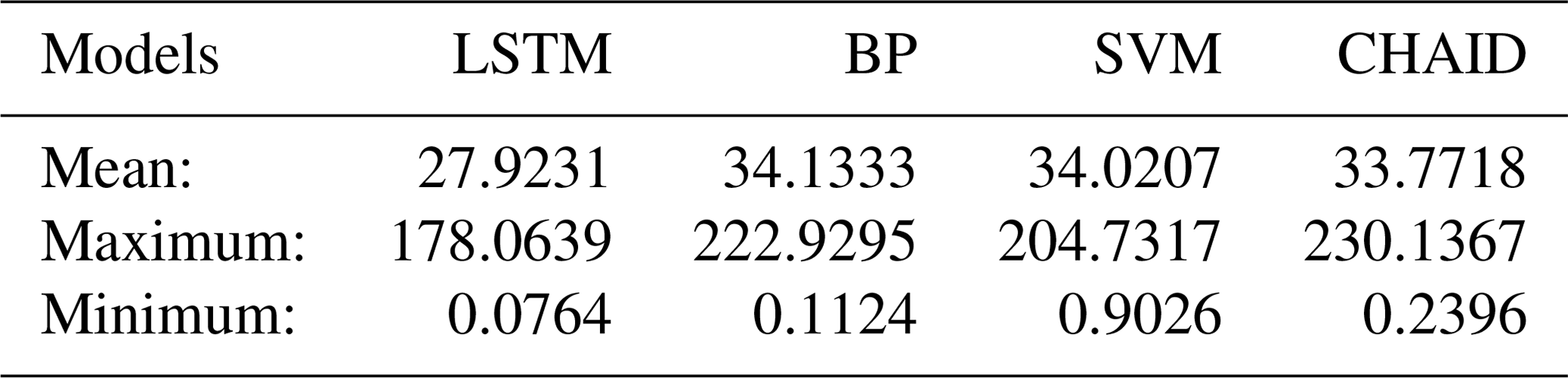
Table 7The results and relative error rates of the random pattern prediction.

5.3 Random pattern prediction
The random pattern prediction randomly selected 12 data points as the outputs among all 590 data points. The randomly selected measured data ranged from 0.2222 to 0.9843, covering the entire range of monitored values. After calculating the prediction results and relative error rates of the four models, the average, maximum, and minimum error rates of the LSTM model were the smallest, and the results were significantly better than those of the other methods (Table 7). The predictions for the maximum and minimum values were also relatively good. However, it could be found that the prediction results obtained by these models were concentrated between 0.35 and 0.75, and the prediction results of the minimum and maximum values were generally poor. The random pattern prediction was based on the completely random selection of time and space aspects and can reflect the effect of air quality prediction under various climatic conditions well. The superiority of the LSTM model prediction in the random prediction pattern was more obvious than in the other patterns, which indicates that under irregular conditions, the LSTM model is more suitable for making predictions.
AOD inversion based on remote sensing technology is being increasingly used for air quality research and is important for monitoring and predicting air quality at a large scale. The proposed PM2.5 ∕ PM10 ratio reflects the air quality and impact of human activities, which is strongest in winter and summer and weakest in spring and autumn. In this paper, we used the DDV method to invert the 59 AOD data points in Wuhan in 2017 based on MODIS images. After the AOD was corrected by the PBLH and RH, the AOD*, which had a greater correlation with PM2.5 ∕ PM10, was obtained, which indicated that the method of correction with the PBLH and RH was effective. After combining gas pollutants and meteorological data, the optimal subset method was used to find the set of factors that were most suitable for the prediction of PM2.5 ∕ PM10. Since the LSTM model uses the gates as switches, better PM2.5 ∕ PM10 prediction results can be obtained. We can also obtain a model that can predict air pollution anytime and anywhere by means of relative factors. Therefore, we set up three prediction patterns: time, space, and random patterns. Among the four intelligent models for comparison, the LSTM model was the most effective, followed by the SVM model, and the CHAID decision tree model was the least effective. The relatively good results of the LSTM model were reflected in not only a higher average prediction accuracy but also the better prediction of maximum and minimum values. Moreover, the accuracy of the LSTM model was more stable. Since LSTM is a time-recurrent neural network that is suitable for processing and predicting events with relatively long intervals and delays in time series, the time pattern prediction results for the three prediction models are the most accurate, and the spatial pattern prediction results without any time data are the least accurate. However, the predictions for the maximum and minimum values were always below average, especially the prediction of the maximum value. The next focuses for improvement will be the optimization of the algorithm and the improvement of the prediction accuracy.
Code content and experimental data can be accessed through the following website: https://doi.org/10.17632/zk9k53zw3z.3 (Wu, 2019).
All authors worked collectively. XW contributed to the conceptualization, methodology, funding acquisition, and project administration; YW contributed to data curation, formal analysis, software, and original draft writing; SH helped perform the analysis with constructive discussions; and ZW partly performed the data curation and processing.
The authors declare that they have no conflict of interest.
We thank David Topping and anonymous referees for their valuable comments.
This study was jointly supported by the Open Fund of Key Laboratory of Urban Land Resources Monitoring and Simulation, MNR (grant no. KF-2019-04-045); the National Natural Science Foundation of China (grant no. 41871355); and the Fundamental Research Funds for the Central Universities, China University of Geosciences (Wuhan) (grant no. CUGQY1936).
This paper was edited by David Topping and reviewed by two anonymous referees.
Arvani, B., Pierce, R. B., Lyapustin, A. I., Wang, Y., and Teggi, S.: Seasonal monitoring and estimation of regional aerosol distribution over Po valley, northern Italy, using a high-resolution MAIAC product, Atmos. Environ., 141, 106–121, 2016.
Bao, G. and Zeng, Z.: Multistability of periodic delayed recurrent neural network with memristors, Neural Comput. Appl., 23, 1963–1967, 2013.
Cai, H., Gui, K., and Chen, Q.: Changes in haze trends in the Sichuan-Chongqing region, China, 1980 to 2016, Atmosphere, 9, 277, https://doi.org/10.3390/atmos9070277, 2018.
Chen, Q. X., Yuan, Y., Huang, X., Jiang, Y. Q., and Tan, H. P.: Estimation of surface-level PM2.5, concentration using aerosol optical thickness through aerosol type analysis method, Atmos. Environ., 159, 26–33, 2017.
Chen, Z. Y., Zhang, T. H., Zhang, R., Zhu, Z. M., Ou, C. Q., and Guo, Y.: Estimating PM2.5 concentrations based on non-linear exposure-lag-response associations with aerosol optical depth and meteorological measures, Atmos. Environ., 173, 30–37, 2018.
Chiou-Jye, H. and Ping-Huan, K.: A deep CNN-LSTM model for particulate matter (PM2.5) forecasting in smart cities, Sensors, 18, 2220, https://doi.org/10.3390/s18072220, 2018.
Crutzen, P. J. and Andreae, M. O.: Biomass burning in the tropics: impact on atmospheric chemistry and biogeochemical cycles, Science, 250, 1669–1678, 1990.
Dominici, F., Peng, R. D., Bell, M. L., Pham, L., Mcdermott, A., Zeger, S. L., and Samet, J. M.: Fine particulate air pollution and hospital admission for cardiovascular and respiratory diseases, JAMA-J. Am. Med. Assoc., 295, 1127–1134, 2006.
Gao, L., Li, J., Chen, L., Zhang, L., and Heidinger, A. K.: Retrieval and validation of atmospheric aerosol optical depth from AVHRR over China, IEEE T. Geosci. Remote, 54, 1–12, 2016.
Hidy, G.: Remote sensing of particulate pollution from space: have we reached the promised land?, Air Repair, 59, 642–644, 2009.
Hu, X., Waller, L. A., Lyapustin, A., Wang, Y., and Liu, Y.: Estimating ground-level PM2.5 concentrations in the Southeastern United States using MAIAC AOD retrievals and a two-stage model, Remote Sens. Environ., 140, 220–232, 2014.
Jia, X., Song, X., Shima, M., Tamura, K., Deng, F., and Guo, X.: Effects of fine particulate on heart rate variability in Beijing: a panel study of healthy elderly subjects, Int. Arch. Occ. Env. Hea., 85, 97–107, 2012.
Jiao, L., Xu, G., Xiao, F., Liu, Y., and Zhang, B.: Analyzing the impacts of urban expansion on green fragmentation using constraint gradient analysis, Prof. Geogr., 69, 553–566, https://doi.org/10.1080/00330124.2016.1266947, 2017.
Jung, C. R., Hwang, B. F., and Chen, W. T.: Incorporating long-term satellite-based aerosol optical depth, localized land use data, and meteorological variables to estimate ground-level PM2.5, concentrations in Taiwan from 2005 to 2015, Environ. Pollut., 237, 1000–1010, 2017.
Kim, D., Kim, J., Jeong, J., and Choi, M.: Estimation of health benefits from air-quality improvement using the MODIS AOD dataset in Seoul, Korea, Environ. Res., 173, 452–461, 2019.
Lelieveld, J., Evans, J. S., Fnais, M., Giannadaki, D., and Pozzer, A.: The contribution of outdoor air pollution sources to premature mortality on a global scale, Nature, 525, 367-371, 2015.
Levy, R. C., Mattoo, S., Munchak, L. A., Remer, L. A., Sayer, A. M., Patadia, F., and Hsu, N. C.: The Collection 6 MODIS aerosol products over land and ocean, Atmos. Meas. Tech., 6, 2989–3034, https://doi.org/10.5194/amt-6-2989-2013, 2013.
Li, L., Yang, J., and Wang, Y.: An improved dark object method to retrieve 500m-resolution AOT (aerosol optical thickness) image from MODIS data: a case study in the pearl river delta area, China, ISPRS J. Photogramm., 89, 1–12, 2014.
Ou, Y., Chen, F., Zhao, W., Yan, X., and Zhang, Q.: Landsat 8-based inversion methods for aerosol optical depths in the Beijing area, Atmos. Pollut. Res., 8, 267–274, 2017.
Pei, E., Le, Y., Jiang, D., and Sahli, H.:ultimodal dimensional affect recognition using deep bidirectional long short-term memory recurrent neural networks, in: 2015 International Conference on Affective Computing and Intelligent Interaction (ACII), Xi'an, 21–24 September 2015, 208–214, 2015.
Prados, A. I., Kondragunta, S., Ciren, P., and Knapp, K. R.: Goes aerosol/smoke product (GASP) over north America: comparisons to AERONET and MODIS observations, J. Geophys. Res., 112, D15201, https://doi.org/10.1029/2006jd007968, 2007.
Qingyu, G., Fuchun, L., Liqin, Y., Rui, Z., Yanyan, Y., and Haiping, L.: Spatial-temporal variations and mineral dust fractions in particulate matter mass concentrations in an urban area of northwestern China, J. Environ. Manage., 222, 95–103, 2018.
Sayer, A. M., Hsu, N. C., Bettenhausen, C., and Jeong, M.-J.: Validation and uncertainty estimates for MODIS collection 6 “Deep Blue” aerosol data, J. Geophys. Res.-Atmos., 118, 7864–7872, https://doi.org/10.1002/jgrd.50600, 2013.
Sisler, J. F. and Malm, W. C.: Characteristics of Winter and Summer Aerosol Mass and Light Extinction on the Colorado Plateau, J. Air Waste Manage., 47, 317–330, 1997.
Sowden, M., Mueller, U., and Blake, D.: Review of surface particulate monitoring of dust events using geostationary satellite remote sensing, Atmos. Environ., 183, 154–164, 2018.
Stafoggia, M., Bellander, T., Bucci, S., Davoli, M., de Hoogh, K., de' Donato, F., Gariazzo, C., Lyapustin, A., Michelozzi, P., Renzi, M., Scortichini, M., Shtein, A., Viegi, G., Kloog, I., and Schwartz, J.: Estimation of daily PM10 and PM2.5 concentrations in Italy, 2013–2015, using a spatiotemporal land-use random-forest model, Environ. Int., 124, 170–179, 2019.
Stirnberg, R., Cermak, J., and Andersen, H.: An analysis of factors influencing the relationship between satellite-derived aod and ground-level PM10, Remote Sensing, 10, 1353, https://doi.org/10.3390/rs10091353, 2018.
Su, T., Li, Z., and Kahn, R.: Relationships between the planetary boundary layer height and surface pollutants derived from lidar observations over China: regional pattern and influencing factors, Atmos. Chem. Phys., 18, 15921–15935, https://doi.org/10.5194/acp-18-15921-2018, 2018.
Sugimoto, N., Shimizu, A., and Matsui, I.: A method for estimating the fraction of mineral dust in particulate matter using PM2.5-to-PM10 ratios, Particuology, 28, 114–120, 2015.
Srivastava, S. and Lessmann, S.: A comparative study of LSTM neural networks in forecasting day-ahead global horizontal irradiance with satellite data, Sol. Energy, 162, 232–247, 2018.
Wang, Z., Chen, L., Tao, J., Zhang, Y., and Su, L.: Satellite-based estimation of regional particulate matter (PM) in Beijing using Vertical-and-RH correcting method, Remote Sens. Environ., 114, 50–63, 2010.
Weninger, F., Geiger, Jürgen, WöLlmer, M., Schuller, B., and Rigoll, G.: Feature enhancement by deep LSTM networks for ASR in reverberant multisource environments, Comput. Speech Lang., 28, 888–902, 2014.
Weninger, F., Erdogan, H., Watanabe, S., Vincent, E., and Schuller, B.: Speech Enhancement with LSTM Recurrent Neural Networks and its Application to Noise-Robust ASR, International Conference on Latent Variable Analysis and Signal Separation, Springer International Publishing, 9237, 91–99, 2015.
Wu, S., Deng, F., Niu, J., Huang, Q., Liu, Y., and Guo, X.: Exposures to PM2.5 components and heart rate variability in taxi drivers around the Beijing 2008 Olympic games, Sci. Total Environ., 409, 2478–2485, 2011.
Wu, X.: PM2.5∕PM10 Ratio Prediction Based on a Long Short-term Memory Neural Network in Wuhan, China, https://doi.org/10.17632/zk9k53zw3z.3, 2019.
Xie, P., Liu, X., Liu, Z., Li, T., Zhong, L., and Xiang, Y.: Human health impact of exposure to airborne particulate matter in pearl river delta, China, Water Air Soil Poll., 215, 349–363, 2011.
Xinpeng, T., Sihai, L., Lin, S., and Qiang, L.: Retrieval of aerosol optical depth in the arid or semiarid region of northern Xinjiang, China, Remote Sensing, 10, 197, https://doi.org/10.3390/rs10020197, 2018.
Zhou, X. and Chen, H.: Impact of urbanization-related land use land cover changes and urban morphology changes on the urban heat island phenomenon, Sci. Total Environ., 635, 1467–1476, 2018.