Modular Assessment of Rainfall–Runoff Models Toolbox (MARRMoT) v1.2: an open-source, extendable framework providing implementations of 46 conceptual hydrologic models as continuous state-space formulations

This paper presents the Modular Assessment of Rainfall–Runoff Models Toolbox (MARRMoT): a modular open-source toolbox containing documentation and model code based on 46 existing conceptual hydrologic models. The toolbox is developed in MATLAB and works with Octave. MARRMoT models are based solely on traceable published material and model documentation, not on already-existing computer code. Models are implemented following several good practices of model development: the definition of model equations (the mathematical model) is kept separate from the numerical methods used to solve these equations (the numerical model) to generate clean code that is easy to adjust and debug; the implicit Euler time-stepping scheme is provided as the default option to numerically approximate each model's ordinary differential equations in a more robust way than (common) explicit schemes would; threshold equations are smoothed to avoid discontinuities in the model's objective function space; and the model equations are solved simultaneously, avoiding the physically unrealistic sequential solving of fluxes. Generalized parameter ranges are provided to assist with model inter-comparison studies. In addition to this paper and its Supplement, a user manual is provided together with several workflow scripts that show basic example applications of the toolbox. The toolbox and user manual are available from https://github.com/wknoben/MARRMoT (last access: 30 May 2019; https://doi.org/10.5281/zenodo.3235664). Our main scientific objective in developing this toolbox is to facilitate the inter-comparison of conceptual hydrological model structures which are in widespread use in order to ultimately reduce the uncertainty in model structure selection.

1 Introduction

Rainfall–runoff modelling is useful to extrapolate our hydrologic understanding beyond measurement availability (Beven, 2009, 2012). We can challenge and improve our understanding of the way catchments function through model-based hypothesis testing (Beven, 2002; Clark et al., 2011; Fenicia et al., 2008b; Kirchner, 2006, 2016) and simulate the impact of changes in climatic conditions and catchment characteristics such as land use change (Bathurst et al., 2004; Ewen and Parkin, 1996; Klemeš, 1986; Peel and Blöschl, 2011; Seibert and van Meerveld, 2016; Wagener et al., 2010). Many different modelling approaches are possible, ranging from lumped, empirical, deterministic bucket-style models to distributed, process-oriented, stochastic, 3-D physics-based models (Beven, 2012). Each of these approaches has its own advantages and drawbacks concerning the level of spatial detail, the amount of model “realism” in terms of the processes represented, input data requirements, and computational time. The toolbox presented in this paper uses deterministic, spatially lumped bucket-style models, also referred to as conceptual hydrological models. Note that this definition of a conceptual model is different from the definition used by authors discussing the modelling process, wherein the conceptual model is a step between having a mental, perceptual model of a catchment and the collection of equations referred to as a mathematical or procedural model (e.g. Beven, 2012; Clark and Kavetski, 2010; Gupta et al., 2012; Refsgaard and Henriksen, 2004).

Every application of a rainfall–runoff model is complicated by various aspects of uncertainty (e.g. Beven and Freer, 2001b; Pechlivanidis et al., 2011; Peel and Blöschl, 2011). Uncertainty is introduced during the measurement of model input variables, such as precipitation (e.g. Oudin et al., 2006) and temperature (e.g. Bárdossy and Singh, 2008), and derived variables such as potential evapotranspiration (e.g. Andréassian et al., 2004; Oudin et al., 2005, 2006). Uncertainty is also present in measurements against which model output is compared, such as streamflow (e.g. Di Baldassarre and Montanari, 2009; McMillan et al., 2010), water table depth (e.g. Freer et al., 2004), and water quality (e.g. McMillan et al., 2012). Values of model parameters can be uncertain due to the dependency of “optimal” parameter values on climatic conditions during model calibration (e.g. Coron et al., 2012; Fowler et al., 2016), due to the choice of calibration algorithm (Arsenault et al., 2014), or due to the performance metric used (e.g. Efstratiadis and Koutsoyiannis, 2010; Gupta et al., 2009). Finally, the choice of model structure (i.e. the collection of equations and their internal connections that make up the model) itself is uncertain (Andréassian et al., 2009; Coron et al., 2012; Van Esse et al., 2013; Fenicia et al., 2008a, 2014; Krueger et al., 2010). Currently, a wide variety of models is available. They may be different in spatial and temporal resolution, include different processes, be deterministic or stochastic, be based on top-down or bottom-up philosophies, or be different in some other way. This paper contributes to the investigation of model structure uncertainty of lumped, deterministic conceptual models. We hope to make progress towards answering a core question in hydrologic modelling: out of the overwhelming number of available models, which one is the most appropriate choice for a given catchment?

Conceptual models tend to have low data requirements (catchment-averaged forcing instead of spatially explicit) and are less computationally intensive than spatially explicit models. They are used in both scientific and operational settings (Perrin et al., 2001). A wide range of conceptual model structures exists, e.g. SACRAMENTO (Burnash, 1995; National Weather Service, 2005), TOPMODEL (Beven and Freer, 2001a), SIMHYD (Chiew et al., 2002), the TANK model (Sugawara, 1995), and many more, but there is no clear basis to choose between the different models (Beven, 2012). Models are different in both their internal structure (i.e. which storages are represented and how they are connected) and in their choice of flux equations (i.e. whether and how any given flux is quantified with a mathematical equation). Choosing the right model for a catchment in which hydrological responses are measured is difficult because achieving a “good” value on a performance metric is a necessary but not sufficient condition to determine whether a model produces the “right results for the right reasons” (Kirchner, 2006). Different model structures can achieve superficially similar performance metrics but might reach this point through wildly different internal dynamics (de Boer-Euser et al., 2017; Goswami and O'Connor, 2010; Perrin et al., 2001). Therefore, good simulation metrics do not necessarily tell us which model structure is more appropriate for this catchment. Choosing a suitable model structure when the catchment is ungauged is even more challenging. This model structure uncertainty is largely unquantified, even for existing models with a long legacy of “successful” (often defined as having achieved a high value for some performance metric) applications. However, comparison of different models can be an expensive task if each model needs to be set up individually. Model inter-comparison studies are further complicated by the fact that documented computer code is unavailable for many model structures.

In recent years multi-model frameworks have received considerable attention. These provide a standardized framework in which several models are presented, users can construct new models, or both. This reduces the time cost of a model comparison study, allows for a fair comparison of different model structures in a test case, and allows the investigator to isolate choices in the model development process. Examples include the Modular Modelling System (MMS; Leavesley et al., 1996), the Rainfall–Runoff Modelling Toolbox (RRMT; Wagener et al., 2002), the Framework for Understanding Structural Errors (Clark et al., 2008), a fuzzy model selection framework (Bai et al., 2009), SUPERFLEX (Fenicia et al., 2011; Kavetski and Fenicia, 2011), the Catchment Modelling Framework (CMF; Kraft et al., 2011), and the Structure for Unifying Multiple Modelling Alternatives (SUMMA; Clark et al., 2015a, b). These frameworks are limited to a small number of existing models (e.g. MMS, RRMT), use a predefined internal organization of stores (FUSE), consist of generic model elements (i.e. stores, fluxes, and lags) that are not easily recognizable as existing models (e.g. CMF, SUPERFLEX), or are more physics-based and thus difficult to use with conceptual models (e.g. SUMMA). Thus, despite these many existing frameworks, there is a need for a new framework that provides a user-friendly, standardized way to construct and compare existing, widely used conceptual models without constraining the allowed model architecture a priori.

This paper introduces the Modular Assessment of Rainfall–Runoff Models Toolbox (MARRMoT) to fill a gap in the current selection of multi-model frameworks. MARRMoT provides an open-source, easy-to-use, expandable framework that currently includes 46 different conceptual model formulations. This provides all the benefits of a multi-model framework: models are constructed in a modular fashion from separate flux equations, which allows for easy modification of the provided models and expansion of the framework with new models or fluxes; good practices for numerical model solving are implemented as standard options; and all MARRMoT models require and provide standardized inputs and outputs. The large number of models in the framework will facilitate studies that lead to more generalizable conclusions about model and/or catchment functioning. This work also provides a pragmatic overview of the wide variety of different flux equations and model structures that are currently used, facilitating studies and discussion beyond direct model comparison. Due to the code being open source, transparency and repeatability of research are encouraged, additions to the framework are possible, and the community can find and correct any mistakes. Finally, MARRMoT is provided with extensive documentation about the models included, the conversion of flux equations to computer code, recommendations for generalized parameter ranges for model sensitivity analysis and/or calibration, a user manual explaining framework setup, functioning, and use, and several example workflow scripts that make the use of the framework possible even with minimal programming experience.

2 MARRMoT design considerations

MARRMoT takes inspiration from earlier modular frameworks (e.g. FUSE, Clark et al., 2008; FLEX, Fenicia et al., 2011) and uses modular code with individual flux equations as the basic building blocks. Multi-model frameworks benefit from modular implementation because this simplifies the programming of the framework and makes it easier to (i) reuse components of a model in a different context, including cases in which the same basic equation is used by multiple models, and (ii) add new options to the framework (Clark et al., 2008). Section 2.1 gives a brief outline of the project scope and design philosophy. MARRMoT follows several good practices for model development which are briefly described in Sect. 2.2 to 2.5.

2.1 Scope

MARRMoT's scope is limited to conceptual hydrological models and the code currently includes no spatial discretization of inputs or catchment response. Models are expected to be used in a lumped fashion, although users could create their own interface to use MARRMoT code to represent within-catchment variability using multiple lumped model structures. Required model inputs are standardized across all MARRMoT models, and every model only requires time series of precipitation, potential evapotranspiration, and optionally temperature (used by certain snow modules). Model outputs are equally standardized and provide time series of simulated flow, total evaporation fluxes, and optionally model states and internal fluxes. The models are set up such that they can use a user-specified time step size (e.g. daily, hourly) which is currently effectively the temporal resolution of the forcing data. Models and flux equations internally account for this time step size so that parameter values can use consistent units, regardless of the temporal resolution of the forcing data. The main goal of this setup is ease of use so that it is straightforward to switch between different model structures within an experiment.

MARRMoT models are based on written documentation only, not on existing computer code. This choice is motivated by our aim to produce traceable code and by several practical concerns. The documentation we base our models on is traceable through our cited sources. Computer code for hydrologic models tends to be less traceable than their documentation: code might be unavailable, code might not be accompanied by a persistent identifier, or multiple versions of the same model (using the same model name) might be available, which complicates finding the “original” computer code. This is supported by various authors who developed the original models: “Today many versions of the HBV model exist, and new codes are constantly developed by different groups ... ” (Lindström et al., 1997); “... TOPMODEL is not a single model structure [...] but more a set of conceptual tools” (Beven et al., 1995).

2.2 Separation of model equations and equation solving

First, MARRMoT uses a distinct separation of model equations as state-space formulations and the numerical approach used to solve these equations. In the theoretical process of developing a new hydrological model, the modeller ideally goes through several distinct steps (e.g. Beven, 2012; Clark and Kavetski, 2010; Gupta et al., 2012). To start, the modeller develops a mental, perceptual model of catchment behaviour based on observations and/or other knowledge (i.e. expert opinion). Next, this model is simplified into an abstraction that shows the connection of the most important fluxes and storages (also termed a conceptual model, but this is a distinctly different meaning than when applied to a bucket-type hydrologic model). These relations are then formalized as ordinary differential equations (ODEs) and their constitutive functions in a mathematical model. Finally, creating computer code to solve these equations sequentially as a time series is done with the procedural model. In practice, however, these stages are often not distinct and tend to overlap (e.g. Kavetski et al., 2003), a process referred to as “ad hoc” modelling. Overlap of the mathematical and procedural model can lead to altered model behaviour and difficulty with parameter estimation (Clark and Kavetski, 2010; Kavetski and Clark, 2010; Kavetski et al., 2003). A clear separation between model equations and the code used to solve those equations gives computer code that is easier to understand and update with new time-stepping schemes or flux equations relative to code into which the model equations are interwoven with the numerical scheme.

2.3 Robust numerical approximation of model equations

Second, MARRMoT gives the possibility to choose a numerical method to approximate the ODEs in discrete time steps. Currently, a fixed-step implicit Euler method is recommended as default, and an explicit Euler method is provided for result matching with previous studies. Many implementations of hydrologic models use the explicit Euler method to approximate storage changes (Schoups et al., 2010; Singh and Woolhiser, 2002). The explicit Euler method relies on storage values at the start of a time step to estimate flux sizes in the current time step: FLUX(t) = f(STORE(t-1)). This method is easy to implement and fast to compute but has several disadvantages: it has low accuracy and only conditional stability, which can lead to large numerical errors and the amplification of such errors under certain conditions (Clark and Kavetski, 2010; Kavetski and Clark, 2010; Schoups et al., 2010). Implicit methods such as implicit Euler instead rely on an iterative procedure that relates flux size to storage at the end of a time step: FLUX(t) = f(STORE(t)). These methods require more intensive iterative computation but avoid the aforementioned issues even when implemented with fixed time step sizes (Kavetski et al., 2006; Schoups et al., 2010). Higher-order numerical approximation methods are currently not provided in MARRMoT but can be included in a straightforward manner. Note that fixed time step size refers to the use of a single time step size throughout a simulation (i.e. no adaptive sub-stepping is used; see Sect. 5.3.5) and does not prescribe the time step size (e.g. hourly, daily)

2.4 Smoothing of threshold discontinuities in model equations

Third, MARRMoT removes threshold discontinuities in model equations through logistic smoothing (Clark et al., 2008; Kavetski and Kuczera, 2007). Hydrologic processes are often characterized by thresholds, e.g. snowmelt starts when a certain temperature is exceeded and saturation excess flow occurs when the soil is saturated. Introducing threshold behaviour into hydrologic models leads to discontinuities in the model's objective function, which can complicate parameter estimation when small changes in parameter values may lead to large changes in objective function value or in the gradient thereof (Kavetski and Kuczera, 2007). Smoothing model equations avoids these discontinuities but also involves a fundamental change to the model equations. Kavetski and Kuczera (2007) recommend logistic functions to smooth threshold equations that closely resemble the original threshold function but are continuous throughout the function's domain. MARRMoT smooths storage-based thresholds with a logistic function (Clark et al., 2008):

$$\begin{array}{}\text{(1)}& {\displaystyle }{Q}_{\mathrm{o}}=Q_{\mathrm{in}}\left(\mathrm{1}-\mathrm{\Phi }\left(S,S_{\max },{\mathit{\rho }}_{\mathrm{S}},\mathit{\epsilon }\right)\right),\text{(2)}& {\displaystyle }\mathrm{\Phi }\left(S,S_{\max },{\mathit{\rho }}_{\mathrm{S}},\mathit{\epsilon }\right)={\displaystyle \frac{\mathrm{1}}{\mathrm{1}+e^{\frac{S-S_{\max }+\mathit{\omega }\mathit{\epsilon }}{\mathit{\omega }}}}},\end{array}$$

where Q_o and Q_in are flux output and input, respectively, and ϕ the smoothing operator. S and S_max are current and maximum storage, respectively, ω represents the degree of smoothing according to ω=ρ_SS_max, and ε is a coefficient that ensures that S does not exceed S_max. ρ_S and ε can be specified by the user or used with default values of 0.01 and 5.00, respectively (Clark et al., 2008). Temperature-based thresholds are smoothed with a different logistic function (Kavetski and Kuczera, 2007):

$$\begin{array}{}\text{(3)}& {\displaystyle }{P}_{\mathrm{S}}=P\mathrm{\Phi }\left(T,T_{\mathrm{t}},{\mathit{\rho }}_{\mathrm{T}}\right),\text{(4)}& {\displaystyle }\mathrm{\Phi }\left(T,T_{\mathrm{0}},{\mathit{\rho }}_{\mathrm{T}}\right)={\displaystyle \frac{\mathrm{1}}{\mathrm{1}+e^{\frac{T-T_{\mathrm{0}}}{{\mathit{\rho }}_{\mathrm{T}}}}}},\end{array}$$

where P_S is precipitation as snow, P incoming precipitation, and ϕ the smoothing operator. T and T₀ are the current and threshold temperatures, respectively, and ρ_T is the smoothing parameter with default value 0.01.

2.5 Simultaneous solving of model equations

Fourth, MARRMoT solves all model equations simultaneously rather than sequentially. Operator-splitting (OS) numerical approximations integrate fluxes sequentially and can be useful in cases such as large systems of partial differential equations, for which computational speed would otherwise be a limiting factor (Fenicia et al., 2011). Sequential calculation of model fluxes is common practice in many hydrologic models (e.g. SACRAMENTO and GR4J), but this approach assumes that fluxes occur in a predetermined order. It is preferable to integrate model fluxes simultaneously to avoid “physically unsatisfying assumption(s)” (Fenicia et al., 2011; Santos et al., 2018). MARRMoT follows this recommendation, barring certain cases in which the model is divided into two distinct parts due to a delay function, in which case simultaneous solving of the first and second part of the model is impossible.

3 MARRMoT

MARRMoT provides MATLAB code for 46 conceptual models following the good model development practices outlined in Sect. 2. This section provides a summary of the framework because it is infeasible to discuss every individual model here. References to the Supplement guide the interested reader to a more in-depth discussion of each model and its implementation in MARRMoT. In addition to this paper, the MARRMoT documentation includes the following.

• Sect. S2: Model descriptions. This document contains descriptions of all 46 models in a standardized format. Each description includes a short introduction to the model, a list of parameters, a model schematic, and a discussion of the ODEs and constitutive functions that describe the model's storage changes and fluxes.

• Sect. S3: Flux equation code. This document contains an overview of the 105 different flux equations used in MARRMoT and their implementation as computer code.

• Sect. S4: Unit hydrograph overview. This document contains an overview of the eight different unit hydrograph routing schemes used in MARRMoT.

• Sect. S5: Parameter ranges. This document contains an overview of recommended parameter ranges for the 46 models based on published literature about hydrologic process and model application studies. The ranges are standardized across models so that similar processes use similar parameter ranges. Use of the recommended ranges is optional.

• User manual: this document helps a user set up MARRMoT for use in either MATLAB or Octave, outlines the inner workings of the standardized models, provides several workflow examples, and provides examples on how to create a new flux equation or model.

3.1 General MARRMoT outline

Figure 1 shows the setup of the MARRMoT framework, including what the framework requires (i.e. data, model options, etc.) and provides for a given modelling study. Each model has its own separate model function, which contains both the numerical implementation of the model (i.e. the ODEs and fluxes that make up this model, as given in Sects. S2, S3, and S4) and the necessary code to handle user input, run the model to produce a time series, and generate output. The user is expected to provide the following inputs: time series of climate variables, initial values for each model store, choice of numerical integration method and settings for MATLAB solvers, and values for each model parameter. Note that the solver selection relates to time-stepping numerics, not parameter selection and/or optimization. Optionally, MARRMoT's provided parameter range guidance (Sect. S5) can inform the choice of parameter values. Parameter ranges have been standardized as much as possible across all models such that similar processes use the same range of possible parameter values across models (e.g. this ensures that all models that have an interception component with a maximum capacity can use the same range, 0–5 mm, for their respective interception capacity parameter). Each model generates a time series of total simulated flow and total simulated evaporation as default output. Optionally, users can request variables with time series of storages and internal fluxes, as well as a summary of the main water balance components. The user manual provides several workflow examples that showcase possible uses of MARRMoT: the examples cover (i) the application of a single model with a single parameter set to a single catchment, (ii) random parameter sampling from provided parameter ranges for a single model, (iii) the application of three different models to a single catchment, and (iv) calibration of a single parameter set for a single model. These examples can easily be adapted to work with multiple catchments if desired.

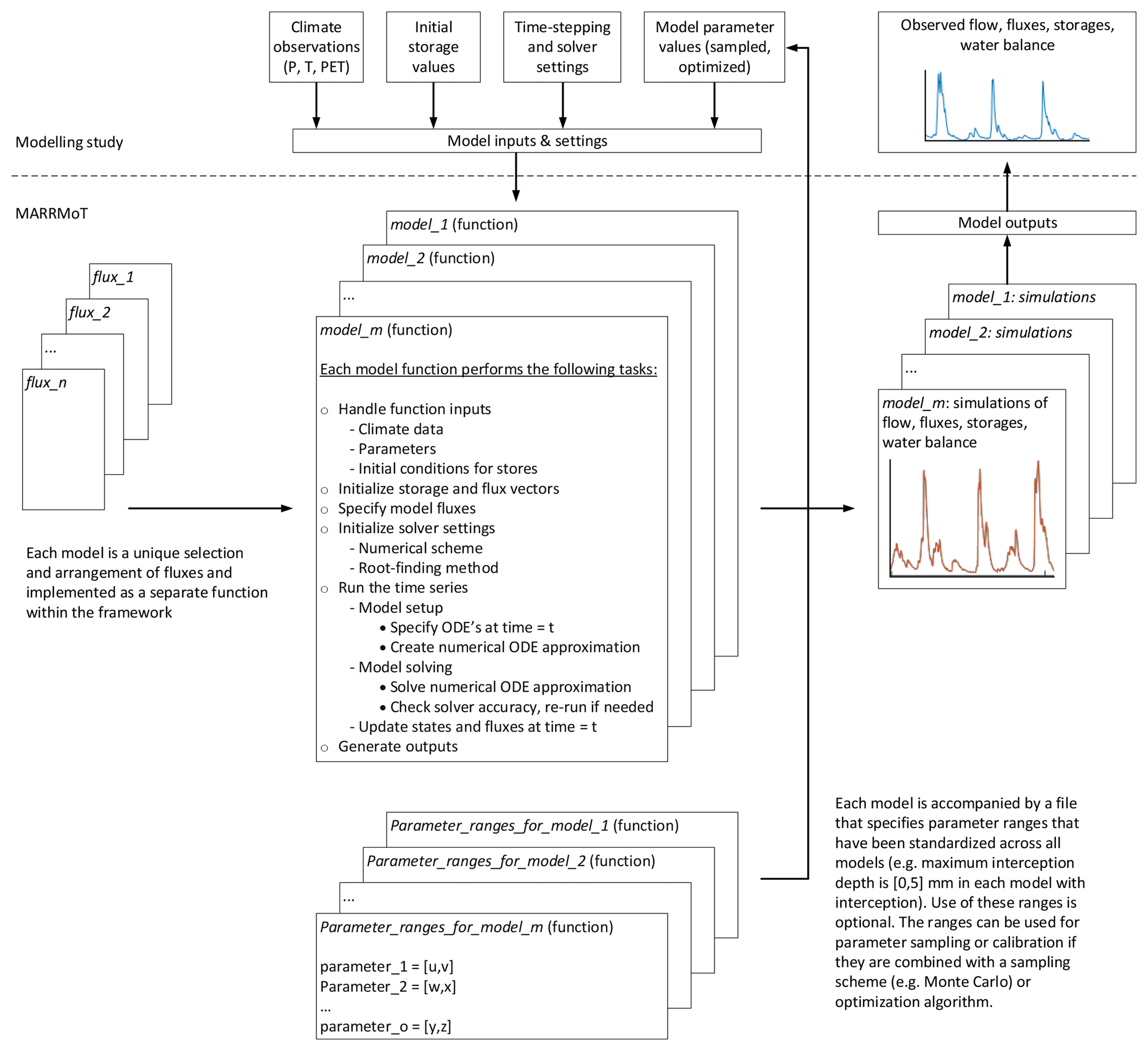
Figure 1 Schematic overview of the MARRMoT framework. MARRMoT provides 46 conceptual models implemented in a standardized way (part below the dotted line). Each model is a unique collection and arrangement of fluxes, but the code-wise setup of each model is the same. Inputs required to run a model are time series of climate variables, values for the model parameters (which can optionally be sampled or optimized using provided, standardized ranges), and initial conditions for each model store. The model returns time series of simulated flow, fluxes, and storages and a summary of the simulated water balance.

The basic building blocks inside each model function are flux functions. Each flux function describes a single flux, for example evaporation from an interception store, water exchange between two soil moisture stores, or baseflow from groundwater. Flux functions are kept separate from the model functions, and each model calls several flux functions as needed. This allows for consistency across models (if errors are present in any flux function, at least they are the same in all models), easy implementation of new flux equations, and facilitation of studies that are specifically interested in differences between various mathematical equations that all represent the same flux or process. The inputs required and output returned by each flux function vary. See Sect. S3 for a full overview of the mathematical functions used to represent fluxes in each model description, relevant constraints, numerical implementation of each flux in MARRMoT, and a list of models that use each flux function. Various models use a unit hydrograph approach to delay flows within the model and/or simulate flow routing. See Sect. S4 for a full overview of the unit hydrographs currently implemented in MARRMoT.

3.2 Summary of included models

Table 1 shows an overview of the model structures currently implemented in MARRMoT and the main reference(s) that these model structures are based on (see Sect. 5.3.3 for a discussion of the comparability of MARRMoT models and their original counterparts). Some of the source models have a long history of application, and others are part of model comparison or development studies. MARRMoT development was not guided by a specific modelling objective (e.g. droughts, floods), and the current selection of model structures mainly aims for variety in the range of model structures. The user manual provides guidance on changing and expanding the framework, and, due to its open nature, these additions can be shared with the wider community. Each model is internally different from the others, either through using different configurations of stores and their connections, through using different flux equations, or both. Models with sequential numbering (e.g. mopex1, mopex2) are part of the same study and tend to be similar but more elaborate as the number increases. Detailed model descriptions can be found in Sect. S2. The model code as currently provided was extensively checked for water balance errors during development using multiple parameter sets for each model, both randomly sampled and using all combinations of extreme values with MARRMoT's provided parameter ranges. These errors were generally of the order of 1E-12 or smaller, showing that the water balance is properly accounted for in each model.

Figure 2 provides a summarized overview of the model differences expressed through the number of stores, number of parameters, and hydrological processes represented. Models use between one and eight stores and between 1 and 23 parameters. The number of parameters tends to increase with the number of stores, but exceptions exist. Most model stores are used to track moisture availability (i.e. across all models 162 stores are used, 155 of which track moisture availability); deficit stores are much rarer (i.e. only 7 out of 162 stores are used to track moisture deficit). Soil moisture storage is the most commonly modelled concept occurring in every model. Routing stores (e.g. “fast flow routing”) are included in 18 models, groundwater stores in 13 models, snow storage in 12, interception in 10, unit hydrograph routing also in 10, surface depression storage in 2, and channel storage in 1 model. However, these numbers should not be seen as representative of all conceptual models because our model overview is necessarily incomplete and some of our models are part of model development studies (wherein a model is modified until satisfactory performance is obtained). These studies skew the number of stores in certain categories.

Table 1 MARRMoT models. Model IDs are used throughout this paper and the MARRMoT documentation. The MARRMoT function names include a longer identifier that either refers to the name of the original model (e.g. m05_ihacres_7p_1s) or to the area of original application (e.g. m_01_collie1_ 1p_1s, which was used in the Collie River basin). The column “Main changes” specifies structural changes between the MARRMoT model and the original model description (note that MARRMoT models are created solely based on the cited sources and not on any computer code). Not mentioned are cases in which (i) model equations needed to be modified to account for the time step size at which the model is used; (ii) ordinary differential equations were not given in the original source; (iii) modelled processes were only described qualitatively in the original source without equations; and/or (iv) model equations were smoothed in their MARRMoT implementations (these can be traced through the overview of flux equations in Sect. S3).

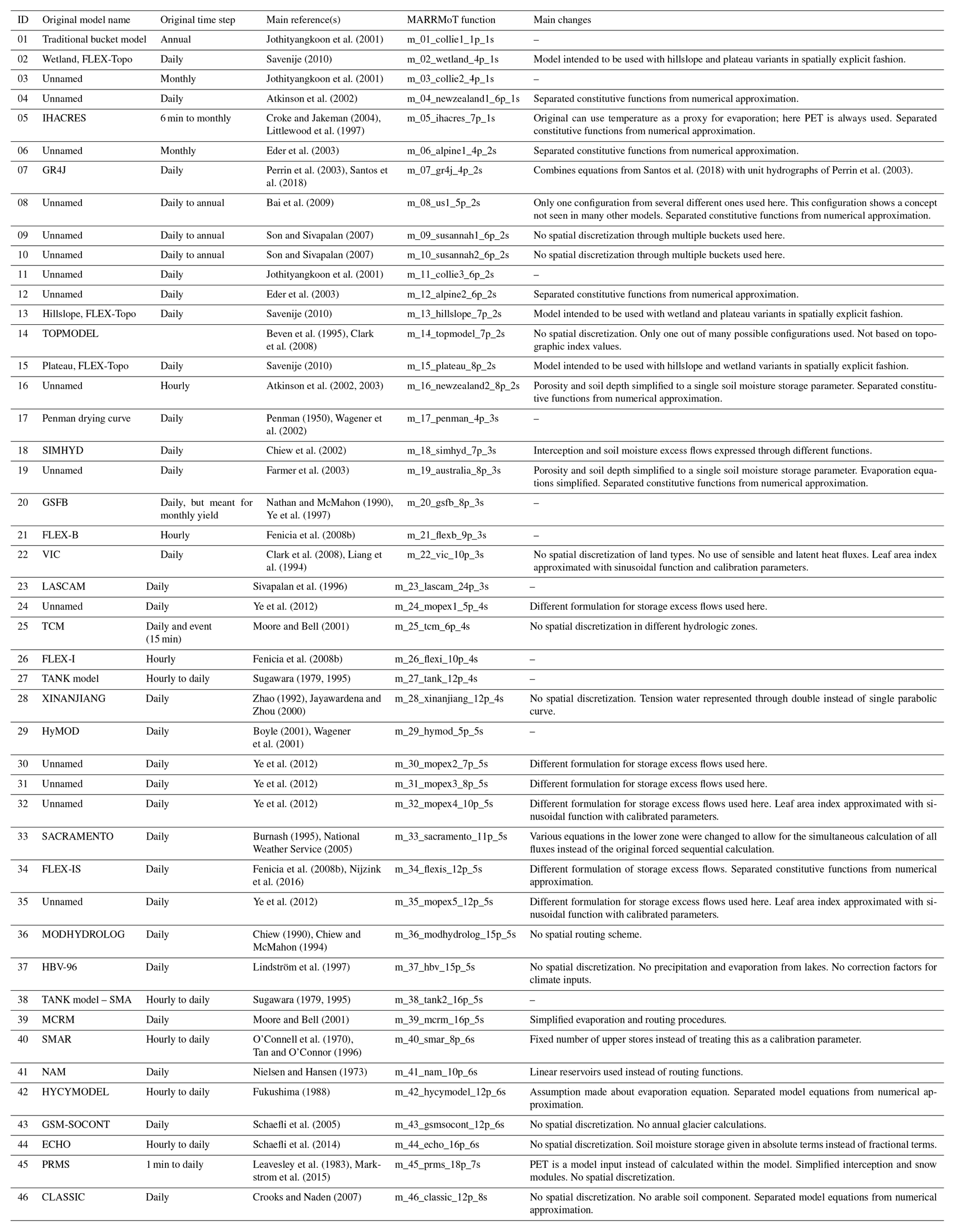
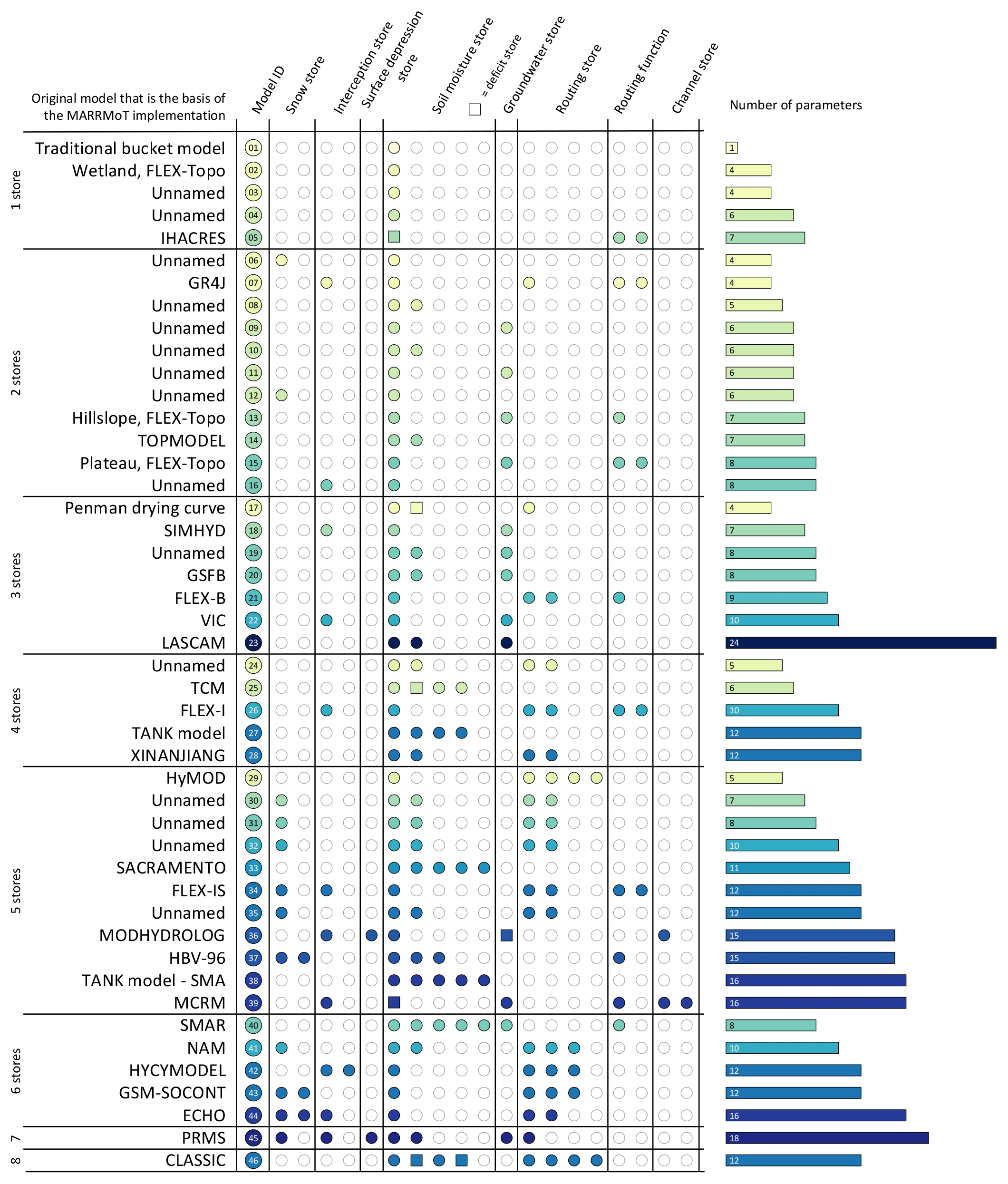
Figure 2 Overview of MARRMoT models. Models are sorted vertically by number of stores (one at the top, eight at the bottom). The columns show broad categories of hydrologic process that can be represented by a model. Coloured circles indicate the model has a store dedicated to the representation of this hydrological process (squares indicate a deficit store). The bar plot on the right shows each model's number of parameters. Colouring refers to the number of parameters.

4 46-model application test case

To demonstrate the potential of the framework, we calibrated all 46 MARRMoT models to flow observations at Hickory Creek near Brownstown, Illinois (USGS ID: 05592575). This catchment was randomly selected from the CAMELS dataset (Addor et al., 2017). The catchment is small, with an area of approximately 115 km², and located at 176 m a.s.l. at latitude 38.9^∘. It has a strong seasonal cycle, with temperatures varying between −20 ^∘C in extreme winters and nearly 30 ^∘C in summers. Average annual rainfall is approximately 1117 mm, 6.4 % of which occurs as snowfall. The runoff ratio is around 29 % of precipitation. The flow regime is flashy (baseflow index is 0.18) and ephemeral (no flow is observed 18 % of the time). High flows (95th percentile flow is 3.7 mm d⁻¹) are more common in winter and spring, while low flows (5th percentile flow is 0 mm d⁻¹) are more common in summer and autumn. Soils are a mixture of silt (60 %), clay (24 %), and sand (16 %).

PET input was estimated using climate data included in CAMELS and the Priestley–Taylor method (Priestley and Taylor, 1972). Model calibration uses the time period 1989–1998, and model evaluation uses the period 1999–2009. Initial states are found by iteratively running each model with data from the year 1989 until model states reach an equilibrium. The calibration algorithm is the covariance matrix adaptation evolution strategy (CMA-ES; Hansen et al., 2003), using the Kling–Gupta efficiency (KGE; Gupta et al., 2009) as the objective function. CMA-ES optimizes a single parameter set per model using MARRMoT's provided parameter ranges. Note that parameter optimization and sampling are currently not part of the provided tools, but connecting MARRMoT to various calibration algorithms or Monte Carlo sampling strategies is straightforward (the user manual provides several basic workflow examples).

Figure 3a shows KGE values during calibration and evaluation for each model. Each result is coloured to indicate the number of calibrated parameters. The number of model parameters seems unrelated to model performance, and several models with higher numbers of parameters are outperformed by the simplest one-parameter bucket model. After analysing the components present in most successful models (not shown), we can speculate that a saturation excess mechanism is key to achieving satisfactory calibration efficiency values in this catchment and that this catchment's flashy behaviour could be related to rainfall events on soil with low available storage.

Figure 3b shows values for two common hydrologic signatures, calculated for time series of simulated flow by each model (blue and white dots, with shading showing the KGE value during calibration) and for observations (red dot). These signatures are calculated for the calibration period. There is significant scatter around the observed signature values, and models with “good” calibration efficiency (darker shades) are not necessarily closer to the observed signature values than models with lower calibration performance. From this we can conclude that even though certain model structures can achieve “high” values for a given objective function, there is no guarantee that the simulated flow series have the same statistical properties as the observed time series the models were calibrated against. Furthermore, this shows that a saturation-excess model can achieve high efficiency values, but the full hydrologic behaviour in this catchment is likely more nuanced than a single runoff generation mechanism.

Note that our findings in this test case are not new, but this test case highlights the power of multi-model comparison frameworks: from two simple plots we have deduced a plausible important runoff mechanism in this catchment, found that this mechanism alone cannot satisfactorily explain the catchment's hydrologic behaviour, and that a higher number of model parameters does not necessarily result in more realistic or better-performing models. Further investigation of the model structures and their performance could lead us to more insights about hydrologic behaviour and inter-model differences, but that is beyond the scope of this test case.

5 Discussion

5.1 Encouraging debate about reproducibility

Reproducibility of computational hydrology is rarely achieved, primarily because data and code are not regularly made available (Hutton et al., 2016). In the case of hydrologic models, this results in many different versions of the same model being in circulation, made either by different people with different interpretations of the original publication and/or including their own model variant. Without publicly available code, only stating a model's name in a study is insufficient for knowing which equations and numerical methods make up that particular instance of the model. Conclusions from any modelling study are thus conditional on a certain set of equations that are unknown to the reader, which makes the generalizability of findings low. However, there is a trend in hydrology towards open and shareable research. Large-scale hydrologic datasets (e.g. CAMELS, Addor et al., 2017; CAMELS-CL, Alvarez-Garreton et al., 2018; GSIM, Do et al., 2018; Gudmundsson et al., 2018) are commonly made available, and certain journals already enforce better coding and sharing practices. Much work is being done on benchmarking data uncertainty (e.g. McMillan et al., 2012) and model performance (e.g. Seibert et al., 2018), which encourages objective conclusions about the strengths and weaknesses of any model and investigation. By making a multi-model toolbox based on various established models available as open-source code, we hope to contribute to this trend of more transparent and reproducible science. Furthermore, this toolbox lowers the threshold for model comparison studies and can help to diminish “legacy” reasons for model application (i.e. choosing to use a certain model for reasons other than the model's perceived appropriateness for the task at hand, such as convenience or past experience; Addor and Melsen, 2019).

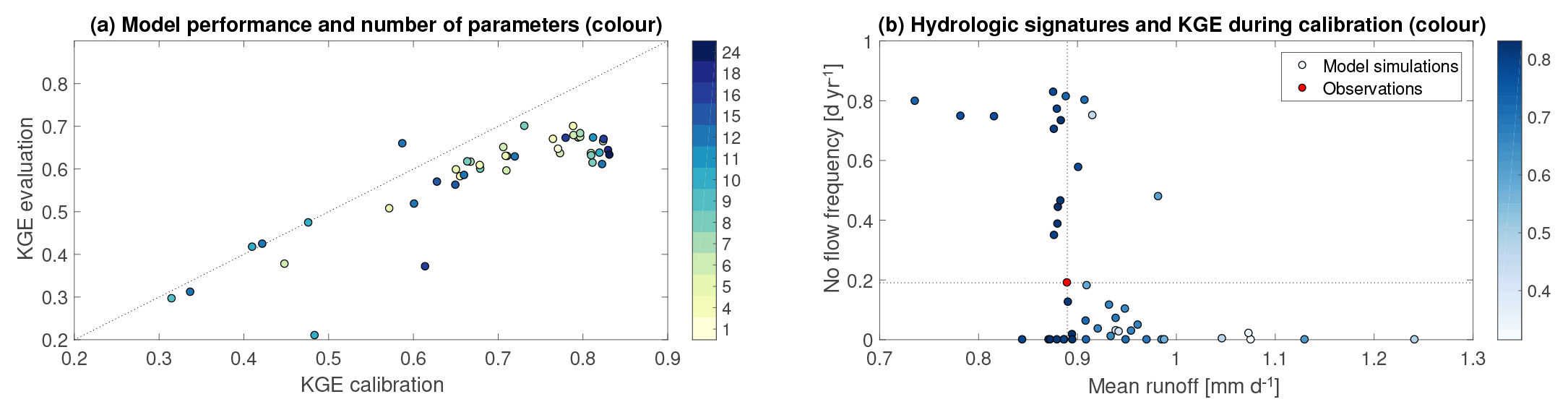
Figure 3 Example of MARRMoT application to Hickory Creek near Brownstown (USA). (a) Model performance during calibration (1989–1998) and evaluation (1999–2009) periods. Each dot represents a single model and is coloured according to the model's number of calibrated parameters. (b) Comparison of simulated average flow and no-flow frequency signature values and observed values for those signatures (red dot bisected with lines).

5.2 The state of conceptual hydrologic models

Our model overview (Sect. S2) and compilation of these models in a single framework allows for unique lessons and insights into the current state of conceptual models (conditional on the sample of model structures we have selected).

The core of this selection of conceptual models is a soil moisture accounting (SMA) module. Every model includes some form of soil moisture store in which moisture is kept and from which moisture is evaporated. Despite this, surface processes, rather than those in the subsurface (both vadose and groundwater zones), tend to be modelled in the greatest detail. For example, intricate snow (e.g. Lindström et al., 1997; Schaefli et al., 2005), interception (e.g. Fukushima, 1988), and surface depression storage (e.g. Chiew and McMahon, 1994; Leavesley et al., 1983; Markstrom et al., 2015) conceptualizations exist among the models, but subsurface processes tend to be much more abstract. This is the same observation as made in Vinogradov et al. (2011). This is understandable because surface processes are easier to observe and formulate hypotheses about, but the subsurface is a crucial component in the water balance (as evidenced by the presence of an SMA component in every single model). A next step in conceptual modelling can be to explicitly formulate hypotheses of subsurface catchment configurations and testing these. For example, the “fill-and-spill” hypothesis (Tromp-Van Meerveld and McDonnell, 2006) could be compared to more traditional subsurface conceptualizations such as linear reservoirs. Framing research as testing alternative hypotheses (Clark et al., 2011) and using modelling tools such as MARRMoT allows for the testing of these ideas in a controlled manner.

A striking difference exists among models that take evaporation from multiple stores. Certain models use the potential evapotranspiration (PET) rate to limit evaporation from each individual store (e.g. MODHYDROLOG, Chiew and McMahon, 1994; NAM, Nielsen and Hansen, 1973; HYCYMODEL, Fukushima, 1988), whereas others use PET as the maximum that can be evaporated from all stores combined (e.g. ECHO, Schaefli et al., 2014; PRMS, Leavesley et al., 1983; Markstrom et al., 2015; CLASSIC, Crooks and Naden, 2007). This can lead to situations in which a model evaporates water at a net rate higher than PET. Depending on the way PET is estimated (see e.g. McMahon et al., 2013, for an overview of PET estimation methods) and which reference crop is used compared to the vegetation in the catchment being modelled, either assumption might be appropriate. Evaporation is a significant component of the water balance (McMahon et al., 2013) and a proper choice in any modelling effort is thus important.

Another difference is the distinction between process-aggregated and process-explicit models. Process-aggregated models (e.g. GR4J, Perrin et al., 2003; IHACRES, Croke and Jakeman, 2004; Littlewood et al., 1997) do not attempt to model individual hydrologic processes but focus on the flows resulting from an aggregation of overall catchment behaviour. Process-explicit models (e.g. MODHYDROLOG, Chiew and McMahon, 1994; FLEX-Topo, Savenije, 2010) explicitly include a variety of hydrologic processes deemed important for a certain modelling purpose. Process-aggregated models tend to have a small number of parameters, which can be preferable when calibrating a model to streamflow only. Process-explicit models are more intuitive when simulating changing conditions due to their explicit process representation, under the strong assumption that the model's equations and parameters can be related to the real-world processes the model intends to simulate.

Summarizing, even within this subset of all hydrologic models, conceptual models exist in a wide variety of shapes and sizes. They are easy-to-use tools to test whether detailed findings from experimental catchments are applicable to many different catchment types worldwide. This approach combines the thorough understanding developed in well-monitored catchments with the ability to generalize conclusions through extensive testing of these findings in other places.

5.3 MARRMoT considerations

5.3.1 Reliance on imperfect methods

MARRMoT uses built-in MATLAB root-finding methods to solve the ODE approximations on every time step. Currently, fzero is the default option for models with one store and fsolve is the default in multi-store models. lsqnonlin is used as a slower but more robust alternative if the former methods are not sufficiently accurate (compared to a user-specified accuracy tolerance). In most cases, this setup performs within acceptable bounds of accuracy. However, for special cases (e.g. very small maximum storage values), the root-finding method might return solutions that are outside the bounds of expected model behaviour (e.g. storages values below 0, storages higher than their maximum capacity, or complex numbers), even if “realistic” solutions also exist. Additional constraints must be introduced into the flux equations to prevent this behaviour because in a large-sample study these issues are difficult to troubleshoot if they occur during the sampling of several thousand combinations of models and catchments. This involves a fundamental change to model equations necessitated by the use of these solvers. More robust solvers such as lsqnonlin allow for the specification of bounds to the solution space but are less computationally efficient. The current trade-off favours constraints implemented into the fluxes and the default use of faster root-finding methods over the more elegant, but much slower, solution provided by lsqnonlin. Further optimization of the root-finding methods is considered outside the scope of this version of MARRMoT. Note that settings for these root-finding methods are specified within each model file because certain settings are model-dependent. Progress display is disabled for all three functions (fzero, fsolve, lsqnonlin) by default but can be enabled by the user. The model-dependent Jacobian matrix is specified for fsolve and lsqnonlin. The maximum number of function evaluations is capped at 1000 for lsqnonlin. All other root-finding options are left at default MATLAB values (see the MATLAB documentation of the root-finding methods for further details). Users are encouraged to experiment with these settings to find those that work for their specific problem.

5.3.2 Speed versus readability

Several considerations during MARRMoT design have been heavily influenced by readability and user-friendliness over computational efficiency. Implementing fluxes as anonymous functions rather than regular functions leads to reduced computational speed but increased clarity of the code.

MATLAB was chosen due to similar concerns. Fortran or a similar compiled language would grant significant speed-ups but reduce user-friendliness.

5.3.3 Correspondence between MARRMoT and original publications

During MARRMoT development, we have tried to stay close to the original publications that introduced the models. Differences are unavoidable, however, due to our criteria of creating a uniform framework. Most changes have to do with spatial discretization, whereby we reduced the level of detail in a model to make all 46 models lumped.

For certain models (e.g. SACRAMENTO; Burnash, 1995; National Weather Service, 2005) model code and numerical implementation are so interwoven that far-reaching changes were required to make these models fit into this generalized framework. For all models, it is likely that the use of the default implicit Euler scheme will provide different results to previous studies that use the (much more common) explicit Euler scheme. Furthermore, the smoothing of model equations will also cause differences to arise with previous studies. We strongly recommend that readers compare the original publication of each model with the version given in this toolbox to place the results from the MARRMoT models in a proper context of earlier work with these models. We emphasize that our models are based on publications that describe existing models, not on existing computer code. Thus, we neither guarantee nor expect that our code performs exactly like the original version of each model's code (if indeed such a version exists and can be found and agreed upon for any given model). To illustrate this point, we compare performance of MARRMoT model m07 (based on the GR4J model) with the R implementation of GR4J (part of the airGR package; Coron et al., 2017, 2019), and we compare MARRMoT model m37 (based on HBV-96) with HBV Light (Seibert and Vis, 2012). MARRMoT m07 is an example of a model that has changed significantly from the original source as a result of combining the original documentation (Perrin et al., 2003) with a more recent state-space version of GR4J (Santos et al., 2018), while both MARRMoT m37 and HBV Light are similar to HBV-96. We thus expect larger deviations between simulations from MARRMoT m07 and airGR-GR4J than we expect between simulations from MARRMoT m37 and HBV Light. In both cases, we selected 10 000 parameter sets from MARRMoT's parameter ranges through Latin hypercube sampling. In the case of GR4J, both MARRMoT and airGR versions use the same four parameters. In the case of HBV, the MARRMoT version has several additional snow parameters and a capillary rise parameter, while HBV Light has various elevation and input correction factors. These have all been fixed at values that effectively disable their impact on model simulations. We then simulated 5 years of streamflow in Hickory Creek (see Sect. 4) using both versions of both models. For comparison purposes, we use the Kling–Gupta efficiency (KGE; Gupta et al., 2009) to express the similarity between simulations and observations. Figure 4 shows the results of this comparison.

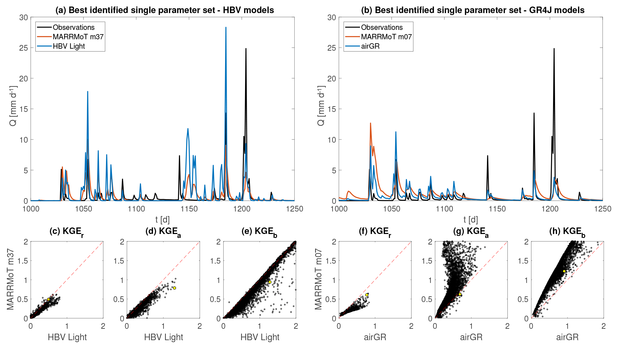
Figure 4 Comparison of two MARRMoT models and freely available model codes based on the same source material. (a) Close-up of hydrographs generated by MARRMoT m37 and HBV Light using the same parameter values for their shared parameters. (b) Close-up of hydrographs generated by MARRMoT m07 and airGR-GR4J using the same parameter values. (c)–(e) Constitutive components of the Kling–Gupta efficiency (KGE) obtained by HBV Light and MARRMoT m37 for 10 000 parameter sets in a single catchment. The yellow dot indicates the parameter set used to generate (a). (f)–(h) Constitutive components of the KGE obtained by airGR-GR4J and MARRMoT m07 for 10 000 parameter sets in a single catchment. The yellow dot indicates the parameter set used to generate (b).

Figure 4a shows that for the best-performing parameter set in our sample (in terms of KGE value), the hydrographs generated by MARRMoT m37 and HBV Light are relatively similar. Figure 4c–e show a decomposition of KGE values into their three constitutive components that express the linear correlation (KGE_r), the ratio of simulated and observed standard deviations (KGE_a), and the ratio of simulated and observed means (KGE_b). For a given parameter set, MARRMoT m37 and HBV Light generate simulations that are relatively similar (i.e. close to the 1:1 line). HBV Light tends to produce more variable flows than MARRMoT m37 (high standard deviation and mean of simulated flows). The reason for this is difficult to investigate because although HBV Light is freely available, its source code is not. Differences between the two models' equations and the numerical approximation of these equations are likely explanations.

Figure 4b shows that for the best-performing parameter set in our sample (in terms of KGE value), the hydrographs generated by MARRMoT m07 and airGR-GR4J are relatively different. Most notable, MARRMoT m07 recessions are much slower and higher than those from airGR-GR4J. Figure 4f–h indicate that for parameter sets close to the optimal points (i.e. (0,0)), MARRMoT m07 and airGR-GR4J show similar performance. For parameter sets further away from the perfect simulation, MARRMoT m07 shows an increasing tendency to simulate more variable flows (higher standard deviation and mean components) than airGR-GR4J. However, differences between MARRMoT m07 and airGR-GR4J are not unexpected because MARRMoT m07 also uses equations from state-space GR4J (Santos et al., 2018) and the models' equations are thus not identical.

Concluding, we emphasize again that MARRMoT models are based on existing publications only and not on computer code. Differences with other models using the same name are unavoidable. We hope that by making MARRMoT available as open-source code, future studies can go beyond simply stating the model name without publishing any model code and can instead refer to an open-source, traceable version of the model(s) used.

5.3.4 Parameter optimization and sampling

MARRMoT provides model code and recommended parameter ranges but does not include any parameter optimization, parameter sampling, or sensitivity analysis methods. This is a conscious choice because these methods continue to be developed and keeping the latest, state-of-the-art version of each packaged in the MARRMoT distribution is infeasible. We refer the reader to e.g. Arsenault et al. (2014) for a recent discussion of various optimization methods, to e.g. Beven and Binley (2014) for a recent discussion of generalized likelihood uncertainty estimation (GLUE), and to e.g. Pianosi et al. (2015) for a recent publication of an open-source sensitivity analysis toolbox. Application of any of these methods with MARRMoT models is straightforward. The user manual provides workflow examples for parameter sampling and parameter calibration, which can be used as a starting point to integrate parameter optimization, sampling, or sensitivity analysis methods.

5.3.5 Possible extensions

Lists of contemporary relevant hydrologic models are hard to come by. Such a list would always be incomplete because new models and model variants continue to be developed. As such, there is no reason to assume that the current 46 models in MARRMoT showcase all possible lumped conceptual hydrologic models. Likewise, although MARRMoT includes a wide variety of flux equations, this list should not be assumed to be complete. The MARRMoT user manual therefore provides detailed guidance on creating new model and flux functions, and the code's location and licensing on GitHub allows these new models to be shared freely. Extensions to the framework are thus possible and encouraged.

Currently lacking in the code is the possibility to use adaptive time stepping. Fixed-step implicit Euler approximations are sufficiently accurate for most applications (Clark and Kavetski, 2010; Kavetski and Clark, 2010; Schoups et al., 2010), but adaptive time stepping can provide additional benefits (Clark et al., 2008; Kavetski and Clark, 2011; Schoups et al., 2010). Our initial assessment is that it would be relatively straightforward to replace the current fixed-step time-stepping implementation with adaptive time stepping (see e.g. Clark and Kavetski, 2010, for further reading on adaptive time stepping).

6 Conclusions

This paper introduces the Modular Assessment of Rainfall–Runoff Models Toolbox (MARRMoT). This modelling framework is based on a review of conceptual hydrologic models. Across these models, over 100 different flux equations and eight different unit hydrographs (UHs) are used. These are implemented as separate functions and each model draws from this library to select the fluxes and UHs it needs. This results in standardized implementations of 46 unique, lumped model structures. The framework is implemented in MATLAB, can be used in Octave, and is provided as open-source software (https://github.com/wknoben/MARRMoT, last access: 30 May 2019; https://doi.org/10.5281/zenodo.3235664). Requirements for running a model are simple: (i) time series of precipitation, potential evapotranspiration, and optionally temperature, (ii) initial storage values, (iii) settings that specify the numerical integration method (currently provided are implicit Euler (recommended) and explicit Euler) and MATLAB solver behaviour, and (iv) values for the model parameters (these can be sampled or optimized from parameter ranges provided as part of MARRMoT). MARRMoT comes with documentation that describes (i) each model and its equations, (ii) the conversion from model equations to computer code, (iii) the implementation of eight different types of unit hydrographs, and (iv) the references used to inform standardized parameter ranges,. The user manual provides guidance on navigating the MATLAB functions in which each model is implemented, several examples of how the framework can be used (with workflow scripts that show the MATLAB code required for these analyses), information on how to create new models or flux functions, and several small modifications that can speed up the model code by disabling certain output messages from MATLAB's built-in solvers. The main purpose of MARRMoT is to enable multi-model comparison studies and objective testing of model hypotheses. Additional benefits can be gained from the framework's documentation, which provides an easy-to-navigate comparison of 46 unique conceptual hydrologic models. MARRMoT is provided to the community in the hopes that it will be useful and to encourage a growing trend of open and reproducible science.