the Creative Commons Attribution 4.0 License.
the Creative Commons Attribution 4.0 License.
 | 29 Mar 2019
Application of random forest regression to the calculation of gas-phase chemistry within the GEOS-Chem chemistry model v10
Christoph A. Keller
Atmospheric chemistry models are a central tool to study the impact of chemical constituents on the environment, vegetation and human health. These models are numerically intense, and previous attempts to reduce the numerical cost of chemistry solvers have not delivered transformative change.
We show here the potential of a machine learning (in this case random forest regression) replacement for the gas-phase chemistry in atmospheric chemistry transport models. Our training data consist of 1 month (July 2013) of output of chemical conditions together with the model physical state, produced from the GEOS-Chem chemistry model v10. From this data set we train random forest regression models to predict the concentration of each transported species after the integrator, based on the physical and chemical conditions before the integrator. The choice of prediction type has a strong impact on the skill of the regression model. We find best results from predicting the change in concentration for long-lived species and the absolute concentration for short-lived species. We also find improvements from a simple implementation of chemical families (NOx = NO + NO2).
We then implement the trained random forest predictors back into GEOS-Chem to replace the numerical integrator. The machine-learning-driven GEOS-Chem model compares well to the standard simulation. For ozone (O3), errors from using the random forests (compared to the reference simulation) grow slowly and after 5 days the normalized mean bias (NMB), root mean square error (RMSE) and R2 are 4.2 %, 35 % and 0.9, respectively; after 30 days the errors increase to 13 %, 67 % and 0.75, respectively. The biases become largest in remote areas such as the tropical Pacific where errors in the chemistry can accumulate with little balancing influence from emissions or deposition. Over polluted regions the model error is less than 10 % and has significant fidelity in following the time series of the full model. Modelled NOx shows similar features, with the most significant errors occurring in remote locations far from recent emissions. For other species such as inorganic bromine species and short-lived nitrogen species, errors become large, with NMB, RMSE and R2 reaching >2100 % >400 % and <0.1, respectively.
This proof-of-concept implementation takes 1.8 times more time than the direct integration of the differential equations, but optimization and software engineering should allow substantial increases in speed. We discuss potential improvements in the implementation, some of its advantages from both a software and hardware perspective, its limitations, and its applicability to operational air quality activities.
- Article
(6251 KB) - Full-text XML
- BibTeX
- EndNote


Atmospheric chemistry is central to many environmental problems, including climate change, air quality degradation, stratospheric ozone loss and ecosystem damage. Atmospheric chemistry models are important tools to understand these issues and to formulate policy. These models solve the three-dimensional system of coupled continuity equations for an ensemble of m species concentrations expressed as number density (molec. cm−3) via operation splitting of transport and local processes:
U denotes the wind vector, (Pi(c)−Li(c)ci) are the local chemical production and loss, Ei is the emission rate, and Di is the deposition rate of species i. We ignore here molecular diffusion as it is negligibly slow compared to advection. The first term of Eq. (1) is the transport operator and involves no coupling between the chemical species. The second term is the chemical operator, which connects the chemical species through a system of simultaneous ordinary differential equations (ODEs) that describe the chemical production and loss:
The numerical solution of Eq. (1) is computationally expensive as the equations are numerically stiff and require implicit integration schemes such as Rosenbrock solvers to guarantee numerical stability (Sandu et al., 1997a, b). As a consequence, 50 %–90 % of the computational cost of an atmospheric chemistry model such as GEOS-Chem can be spent on the integration of the chemical kinetics (Long et al., 2015; Nielsen et al., 2017; Eastham et al., 2018; Hu et al., 2018).
Previous efforts to increase the efficiency of the integration (with an associated reduction in accuracy) have involved dynamical reduction in the chemical mechanism (adaptive solvers) (Santillana et al., 2010; Cariolle et al., 2017), separation of slow and fast species (Young and Boris, 1977), quasi-steady state approximation (Whitehouse et al., 2004a) or approximation of the chemical kinetics using polynomial functions (repro-modelling) (Turányi, 1994). Other approaches have attempted to simplify the chemistry leading to a reduction in the number of reactants and species (Whitehouse et al., 2004b; Jenkin et al., 2008). However, none of these approaches have been transformative in their reduction in time spent on chemistry.
We discuss here the potential of a machine learning algorithm (in this case random forest regression) as an alternative approach to explicitly solving Eq. (1) with a numerical solver in the chemistry model GEOS-Chem. Figure 1 illustrates the approach: during each model time step, GEOS-Chem sequentially solves a suite of operations relevant to the simulation of atmospheric chemistry. In the original model, solving the chemistry is the computationally most expensive step. Our aim is to replace it with a machine learning algorithm while keeping all other processes unchanged. Conceptually, this approach is comparable to previous efforts to speed up the solution of the chemical equations through more efficient integration.

Figure 1Schematic overview of the use of a random forest regression algorithm as an alternative to the chemistry solver. The original numerical model (GEOS-Chem) sequentially solves the operations relevant to atmospheric chemistry, with the chemical integrator being the computationally most expensive step (left side). Using training data produced from the full model, we generate a machine learning emulator that can then be used instead of the chemical integrator (right side). All other model processes are the same as in the original model.
Machine learning is becoming increasingly popular within the natural sciences (Mjolsness and DeCoste, 2001) and specifically within the Earth system sciences to either simulate processes that are poorly understood or to emulate computationally demanding physical processes (notably convection) (Krasnopolsky et al., 2005, 2010; Krasnopolsky, 2007; Jiang et al., 2018; Gentine et al., 2018; Brenowitz and Bretherton, 2018). Machine learning has also been used to replace the chemical integrator for other chemical systems such as those found in combustion and been shown to be faster than solving the ODEs (Blasco et al., 1998; Porumbel et al., 2014). Recently, Kelp et al. (2018) found order-of-magnitude speed-ups for an atmospheric chemistry box model using a neural network emulator, although their solution suffers from rapid error propagation when applied over multiple time steps. Machine learning emulators have also been explored to directly predict air pollution concentration in future time steps (Mallet et al., 2009), as well as for chemistry–climate simulations focusing on model predictions of time-averaged concentrations for selected species such as ozone (O3) and the hydroxyl radical (OH) over timescales of days to months (Nicely et al., 2017; Nowack et al., 2018). In contrast, the algorithm presented here is optimized to capture the small-scale variability of the entire chemical space within a timescale of minutes, with only a small loss of accuracy when used repeatedly over multiple time steps. To do so, we use the numerical solution of the GEOS-Chem chemistry model to produce a training data set of output before and after the chemical integrator (Sect. 2.1 and 2.2), train a machine learning algorithm to emulate this integration (Sect. 2.3, 2.4 and 2.5), and then describe and assess the trained machine learning predictors (Sect. 2.6, 2.7, 2.8 and 2.9). Section 3 describes the results of using the machine learning predictors to replace the chemical integrator in GEOS-Chem. In Sect. 4 we discuss potential future directions for the uses of this methodology and in Sect. 5 we draw some conclusions.
2.1 Chemistry model description
All model simulations were performed using the NASA Goddard Earth Observing System Model, version 5 (GEOS-5) with version 10 of the GEOS-Chem chemistry embedded (Long et al., 2015; Hu et al., 2018). GEOS-Chem (http://geos-chem.org, last access: 18 March 2019) is an open-source global model of atmospheric chemistry that is used for a wide range of science and operational applications. The code is freely available through an open license (http://acmg.seas.harvard.edu/geos/geos_licensing.html, last access: 18 March 2019). Simulations were performed on the Discover supercomputing cluster of the NASA Center for Climate Simulation (https://www.nccs.nasa.gov/services/discover, last access: 18 March 2019) at cube sphere C48 horizontal resolution, roughly equivalent to 200 km×200 km. The vertical grid comprises 72 hybrid-sigma vertical levels extending up to 0.01 hPa. The model uses an internal dynamic and chemical time step of 15 min.
The model chemistry scheme includes detailed tropospheric chemistry of oxides of hydrogen, nitrogen, bromine, volatile organic compounds and ozone (HOx–NOx–BrOx–VOC–ozone), as originally described by Bey et al. (2001), with the addition of halogen chemistry by Parrella et al. (2012) plus updates to isoprene oxidation as described by Mao et al. (2013). Photolysis rates are computed online by GEOS-Chem using the Fast-JX code of Bian and Prather (2002) as implemented in GEOS-Chem by Mao et al. (2010) and Eastham et al. (2014). The gas-phase mechanism comprises 150 chemical species and 401 reactions and is solved using the kinetic pre-processor (KPP) Rosenbrock solver (Sandu and Sander, 2006). There are 99 (very) short-lived species which are not transported, and we seek to emulate the evolution of the other 51 transported species.
While the GEOS model with GEOS-Chem chemistry can be run as a chemistry–climate model where the chemical constituents (notably ozone and aerosols) directly feed back to the meteorology, we disable this option here and use prescribed ozone and aerosol concentrations for the meteorology instead. This ensures that any differences between the reference model and the machine learning model can be attributed to imperfections in the emulator rather than changes in meteorology due to chemistry–climate feedbacks.
2.2 Training data
To produce our training data set we run the model for 1 month (July 2013). Each hour we output the three-dimensional instantaneous concentrations of each transported species immediately before and after chemical integration, along with a suite of environmental variables that are known to impact chemistry: temperature, pressure, relative humidity, air density, cosine of the solar zenith angle, cloud liquid water and cloud ice water. In addition, we output all photolysis rates since those are an essential element for chemistry calculations. Alternatively, one could also envision directly embedding the (computationally demanding) photolysis computation into the machine learning model, such that the emulator takes as input variables additional environmental variables relevant to photolysis (e.g. cloud cover, overhead ozone and aerosol loadings) and then emulates photolysis computation along with chemistry.
Each grid cell 1 h output constitutes one training sample, consisting of 126 input “features”: the 51 transported species concentrations, 68 photolysis rates and the 7 meteorological variables. We restrict our analysis to the troposphere (lowest 25 model levels) since this is the focus of this work. Each hour thus produces a total of 327 600 training samples, and so an overall data set of 2.4×10⁸ samples is produced over the full month. We withhold a randomly selected 10 % of the samples to act as validation data while the remaining samples act as training data.
2.3 Random forest regression
We use the random forest regression (RFR) algorithm (Breiman, 2001) to emulate the integration of atmospheric chemistry. Figure 2 shows a schematic of RFR. It is a commonly used, and conceptually simple, supervised learning algorithm that consists of an ensemble (or forest) of decision trees. Each tree contains a tree-like sequence of decision nodes, based on which the tree splits into its various branches until the end of the tree (“the leaf”) is reached. This leaf is the prediction of the decision tree. Each decision node is based on whether one of the input features is above a certain value. An important aspect of the random forest is that each tree of the forest is trained on a subset of the full training data, thus providing a slightly different approximation of the model. A prediction is then made by averaging the predictions of the individual trees.
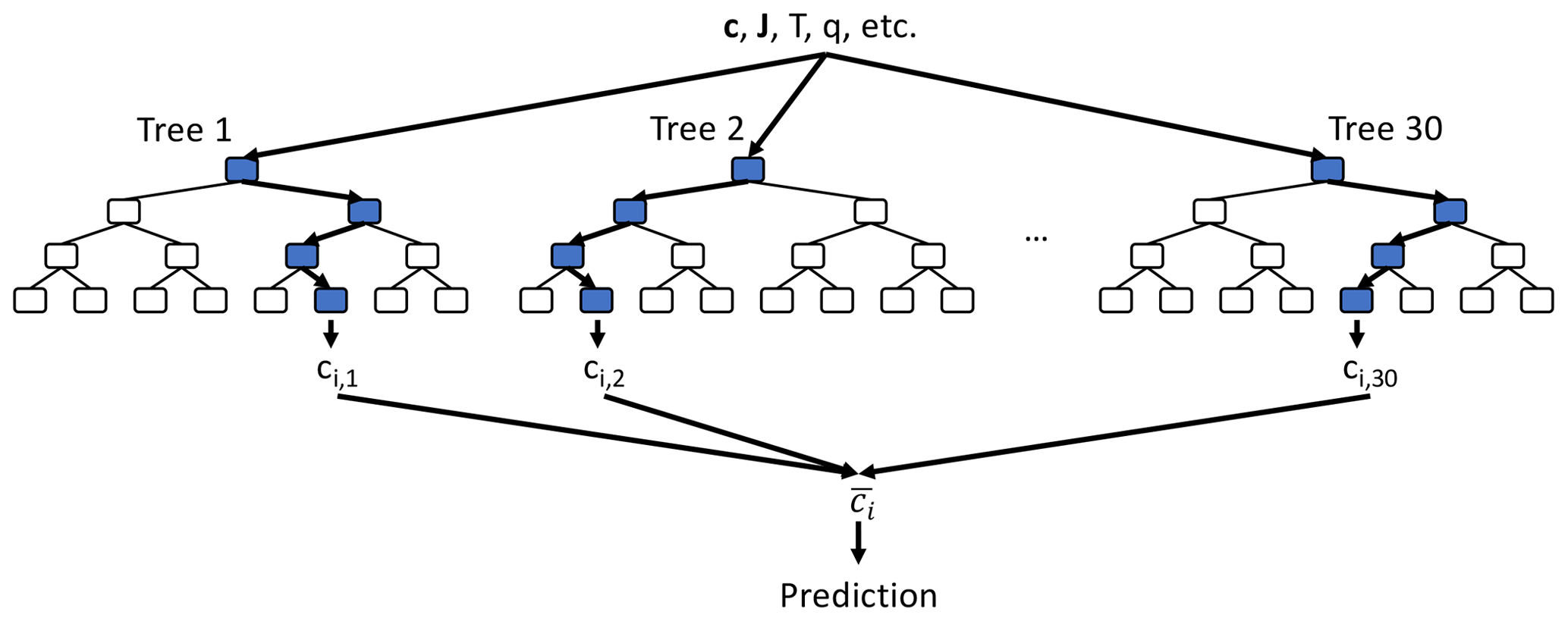
Figure 2Schematic of random forest algorithm. For each species ci, we use a random forest consisting of 30 individual decision trees, each up to 12 layers deep (only the first four layers are shown). All decision trees take the same inputs (e.g. species concentration vector c at given location, photolysis rates J, temperature T, humidity q) and each decision tree node uses one of the input features plus a threshold value to determine the tree path for the given set of input features. The final prediction is made by averaging the 30 individual tree predictions ().
The RFR algorithm is less prone to over-fitting and produces predictions that are more stable than a single decision tree (Breiman, 2001). Random forests are widely used since they are relatively simple to apply, suitable for both classification and regression problems, do not require data transformation, and are less susceptible to irrelevant or highly correlated input features. In addition, random forests allow for easy evaluation of the factors controlling the prediction, the decision structure and the relative importance of each input variable. Analysing these features can offer valuable insights into the control factors of the underlying mechanism, as discussed later. We discuss the potential for other algorithms in Sect. 4.
2.4 Implementation
For each of the 51 chemical species transported in the chemistry model, we generate a separate random forest predictor. This predictor can be applied to all model grid cells, i.e. it captures all chemical regimes encountered by the respective target species. Conceptually, one can imagine that each tree path represents a different chemical regime, so it is important to generate trees that are large enough to encompass the entire solution space. We find a good compromise between computational complexity and accuracy of the solutions for random forests consisting of 30 trees with a maximum of 10 000 leaves (prediction values) per tree. These hyper-parameter were determined by trial and error, and we find very little sensitivity of our results to changes (±50 %) to the number of trees and/or number of leaves. Each tree is trained on a different sub-sample of the training data by randomly selecting 10 % of the training sample. In order to balance the training samples across the full range of model values, the training samples are evenly drawn from each decile of the predictor variable. This prevents over-sampling of ocean grid cells, which are typically characterized by very uniform chemistry. Our results show very little sensitivity to the size of the training sample as long as it covers the full solution space.
The Python software package scikit-learn (http://scikit-learn.org/stable/, last access: 18 March 2019) (Pedregosa et al., 2011) was used to build the forests. We distributed the training of the entire forest (30 trees for 51 species) onto 1530 CPUs, and each tree took 1 h to train. After training, all forest data (i.e. all tree node decisions and leaf values) were written into text files.
The forests were then embedded as a Fortran 90 subroutine into the GEOS-Chem chemistry module. Using an ad-hoc approach, the module first loads all tree nodes (archived after the training) into local memory and then evaluates each of the 1530 trees in series upon calling the random forest emulator. Each grid cell calls the same random forest emulator separately, passing to it all local information required to evaluate the trees (species concentrations, photolysis rates, environmental variables). No attempts were made to optimize the prediction algorithm beyond the existing Message Passing Interface grid-domain splitting.
2.5 Choice of predictor
We find that the quality of the RFR model (as implemented back into the GEOS-Chem model) depends critically on the choice of the predictor. Most simplistically, we could predict the concentration of a species after the integration step. However, many of the species in the model are log-normally distributed in which case predicting the logarithm of the concentration may provide a more accurate solution; we could also predict the change in the concentration after the integrator, the fractional change in the concentration, the logarithm of the fractional change, etc. After some trial and error, and based on chemical considerations, we choose two types of prediction: the change in concentration after going through the integrator, and the concentration after the integrator. We describe the first as the “tendency”. This fits with the differential equation perspective for chemistry given in Eq. (1). However, if we incorporate only this approach we find that errors rapidly accrue. This is due to errors in the prediction of short-lived species such as NO, NO3 and Br. For these compounds, concentrations can vary by many orders of magnitude over an hour, and even small errors in the tendencies build up quickly when they are included in the full model. For these short-lived compounds, we use a second type of prediction where the RFR predicts the concentration of the compound after the integrator. We describe this as a prediction of the “concentration”. From a chemical perspective, this is similar to placing the species into steady state, where the concentration after the integrator does not depend on the initial concentration but is a function of the production (P) and loss (L⋅c) such that . We imitate this process by explicitly removing the predictor species from the input features, which we find improves performance.
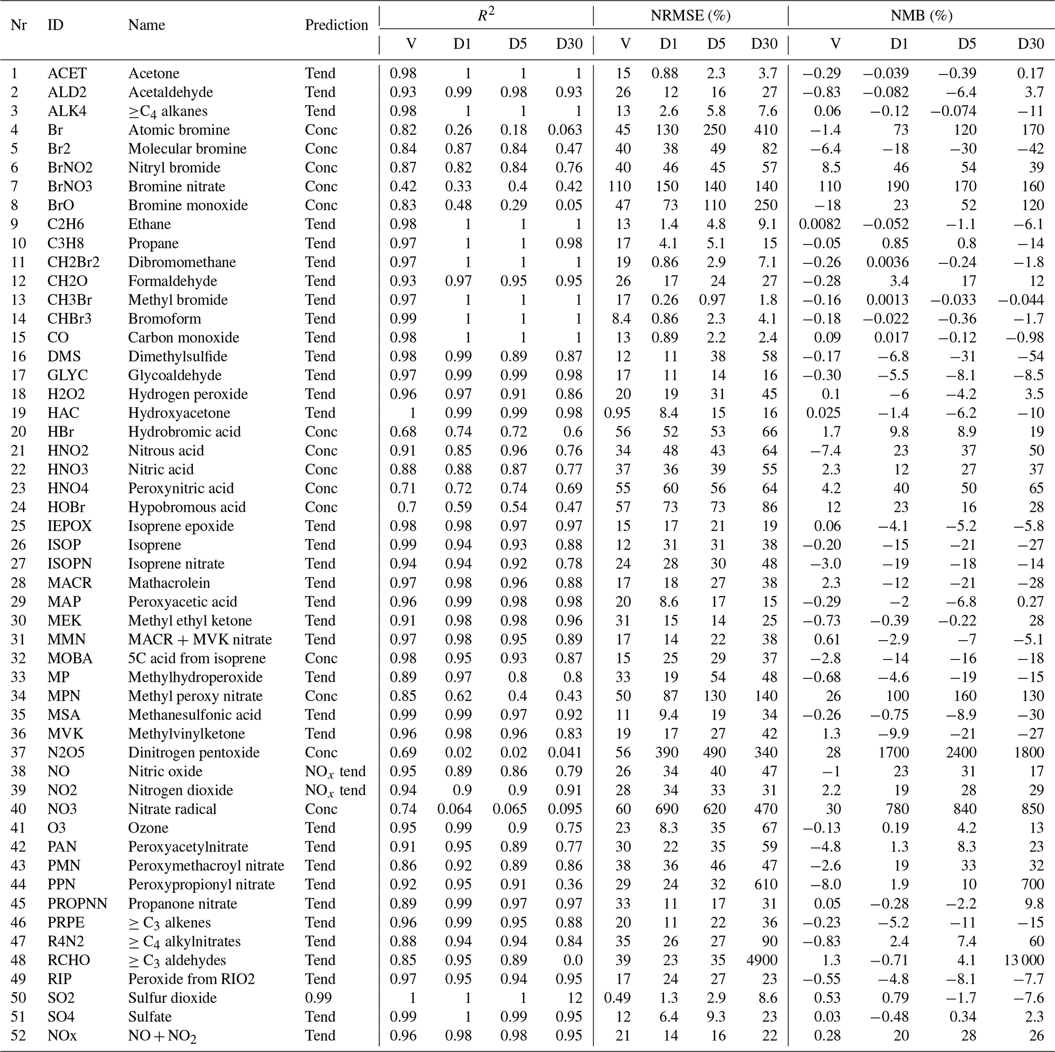
The choice between predicting the tendency or the concentration is based on the standard deviation of the ratio of the concentration after chemistry to the concentration before chemistry (σ(c∕c0)) in the training data. This ratio is relatively stable and close to 1.00 for long-lived species but highly variable for short-lived species. Based on trial and error, we use a standard deviation threshold of 0.1 to distinguish between long-lived species (σ<0.1) and short-lived species (σ≥0.1). Table 1 lists the prediction type used for each species. We discuss the treatment of NO and NO2 species in Sect. 2.7.
Table 1Overview of the performance of the RFR model with the NOx family treatment. Shown are the Pearson correlation R2, normalized root mean square error (NRMSE) and normalized mean bias (NMB). Comparison against the validation data set (10 % of training data withheld from training) are indicated with a “V”. Comparisons between the RFR simulation and the full GEOS-Chem model for July 2014 at 00:00 UTC after the 1st, 5th and 30st simulation day are indicated with “D1”, “D5” and “D30”, respectively. Prediction type of each species (concentration, tendency, NOx family treatment) is given in the prediction column.
2.6 Feature importance
The importance of different input variables (features) for making a prediction of O3 tendency is shown in Fig. 3a. The importance metric is the fraction of decisions in the forest that are made using a particular feature, with the variability indicating the standard deviation of that value between the trees. Consistent with our understanding of atmospheric chemistry, features such as NO, formaldehyde (CH2O), the cosine of the solar zenith angle (“SUNCOS”), bromine species and nitrogen reservoirs all appear within the top 20. From a chemical perspective, these features make sense given the global sources and sinks of O3 in the lower to middle troposphere.
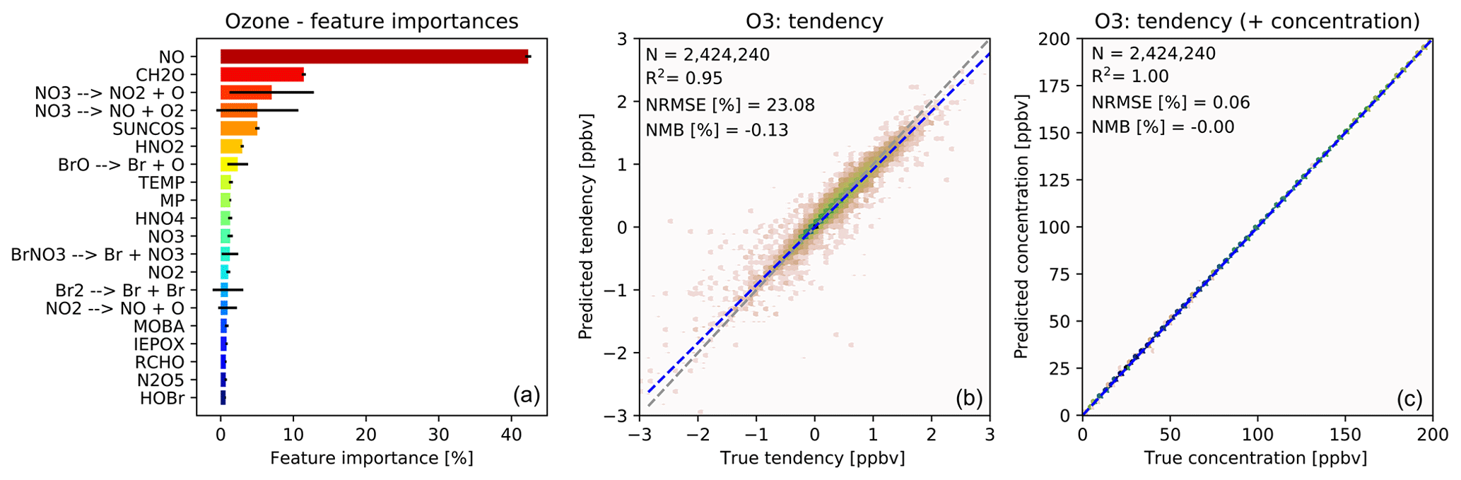
Figure 3Characteristics of random forest trained to predict tendencies of O3 due to chemistry. (a) Importance of input variables (features) for random forests trained to predict tendency of ozone due to chemistry. Shown are the 20 most important features for the entire random forest, as averaged over all 30 decision trees. The black bars indicate the standard deviation for each feature across the 30 decision trees. The arrows indicate photolytic conversion (i.e. NO3 photolyses to NO2 plus O). (b) Validation of random forest prediction skill for ozone: comparison of ozone tendency validation data (x axis) vs. predicted values (y axis). Number of validation points (N), correlation coefficient (R2), normalized root mean square error (NRMSE) and normalized mean bias (NMB) are given in the inset. (c) Same validation but with tendency added to the concentration before integration.
For ozone prediction, 6 out of the 20 most important input features are related to photolysis. Most of the photolysis rates are highly correlated, and the individual decision trees use different photolysis rates for decision making. This results in very large standard deviations for the photolysis input features across the 30 decision trees, as indicated by the black bars in Fig. 3a.
Note that the concentration of O3 is not among the 20 most important input features for the prediction of O3 tendency. If, instead, the random forest model is trained to predict the concentration of O3, the initial O3 concentration dominates the input feature importance, explaining more than 99 % of the prediction. However, when predicting the ozone tendency, the random forest algorithm is more sensitive to availability of NOx, VOCs, photolysis, etc., rather than the initial concentration of O3. For regions producing ozone (dominated by the reaction) the O3 concentration is not the primary source of variability. Similarly, for regions loosing ozone the dominant source of variability is the variability in photolysis rates (multiple orders of magnitude) rather than the variability in O3 concentration (less than an order of magnitude).
Fig. 3b shows the performance of the O3 tendency predictor against the validation data. The predictor is not perfect, with an R2 of 0.95 and a normalized root mean square error (NRMSE) of 23 %, but it is essentially unbiased with a normalized mean bias (NMB) of −0.13 % (descriptions of the metrics can be found in Sect. 2.8). However, as shown in Fig. 3c, the model becomes almost perfect when the tendency is added to the initial concentration – which is the operation to be performed by the chemistry model.
2.7 Prediction of NOx
For NO and NO2 we find that the random forest has difficulties predicting the species concentrations independently of each other. This can result in unrealistically large changes in total NOx (). Given the central role of NOx for tropospheric chemistry, a quick deterioration of model performance occurs (see Sect. 3.1). For these species we thus adopt a different methodology: instead of making predictions for the species individually, we predict the tendency for a family comprising their sum (NO + NO2) and then predict the ratio of NO to NOx. NO2 is then calculated by subtracting NO from NOx. Thus, the overall number of forests that needs to be calculated does not change. This has the advantage of treating NOx as a long-lived family “species” and includes a basic conservation law, but it allows the NO and NO2 concentration to still vary rapidly.
Figure 4 shows the feature importance and the comparison with the validation data for the prediction of the NOx family tendency. The features make chemical sense, with NO2 and NO but also acetaldehyde (a tracer of PAN chemistry) and HNO2, a short-lived nitrogen species, playing important roles. The importance of SO2 may reflect heterogeneous N2O5 chemistry, with SO2 being a proxy for available aerosol surface area (note that we do not provide any aerosol information to the RFR). As shown in Fig. 4b, the NOx predictor gives the “true” NOx tendencies from the validation data with an R2 of 0.96, NRMSE of 21 % and NMB of 0.28 %. While the NRMSE is relatively high, we find that the ability of the model to produce an essentially unbiased prediction is more critical for the long-term stability of the model. As for O3, the NOx skill scores become almost perfect when adding the tendency perturbations to the concentration before integration (Fig. 4c).
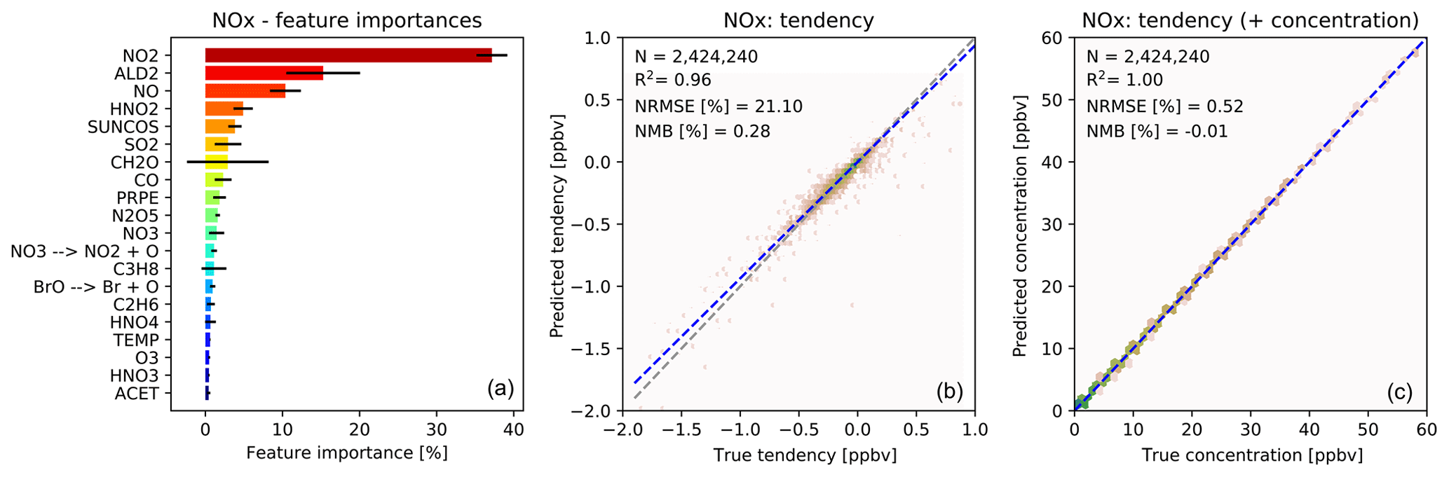
Figure 5 shows the feature importance and performance of the predictor for the ratio of NO to NOx. Again the features make chemical sense with the top three features (photolysis, temperature and O3) being those necessary to calculate the NO-to-NO2 ratio from the well known Leighton relationship (Leighton, 1961). The performance of the NO-to-NOx ratio predictor is very good, and the prediction is also unbiased.
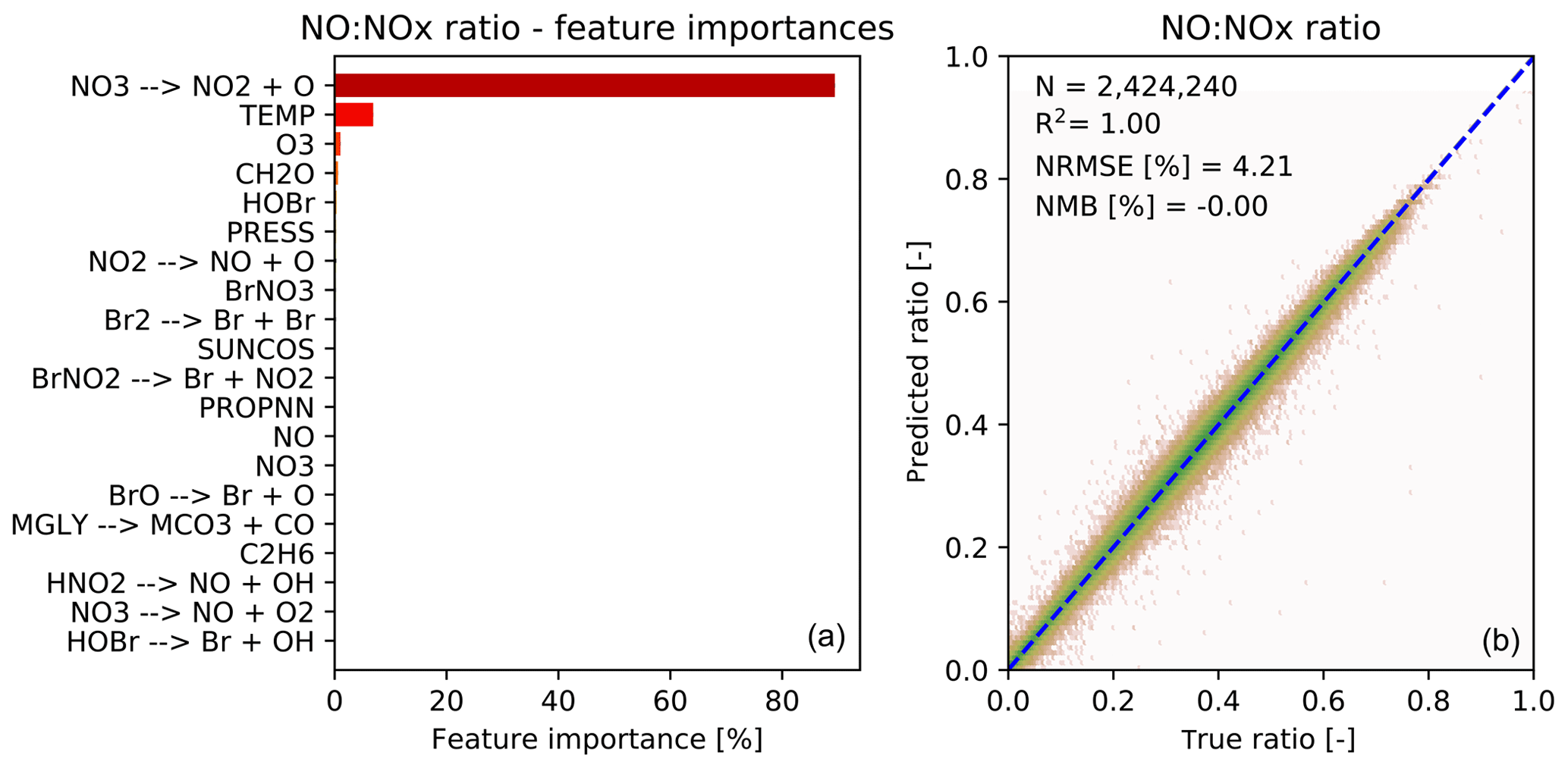
Figure 5Characteristics of random forest trained to predict the NO∕NOx ratio after chemistry. (a) 20 most important features for the NO∕NOx random forest, as averaged over all 30 decision trees. The black bars indicate the standard deviation of the feature importance; (b) Comparison of predicted NO∕NOx ratios (y axis) vs. true NO∕NOx ratios (x axis) for the validation data (not used for training). Number of validation points (N), correlation coefficient (R2), normalized root mean square error (NRMSE) and normalized mean bias (NMB) are given in the inset.
2.8 Evaluation metrics
We now move to a systematic evaluation of the performance of the RFR models, both against the validation data and when implemented back into the GEOS-Chem model. We use three standard statistical metrics for this comparison. For each species c, we compute the Pearson correlation coefficent (R2),
the root mean square error normalized by the standard deviation σ (NRMSE),
and the normalized mean bias (NMB):
where denotes the concentration predicted by the RFR model, c is the concentration calculated by GEOS-Chem, and N is the total number of grid cells.
2.9 Performance against the validation data
Ten percent of the training data was withheld to form a validation data set. Columns “V” in Table 1 provide an evaluation of each predictor against the validation data for the three metrics discussed in Sect. 2.8. For most species the RFR predictors do a good job of prediction: R2 values are greater than 0.90 for 35 of the 51 species, NRMSEs are below 20 % for 21 species and NMBs are below 1 % for 29 species, respectively. Those species which do less well are typically those that are shorter lived, such as inorganic bromine species or some nitrogen species (NO3, N2O5). The performance of NO and NO2 after implementing the NOx family and ratio methodology is consistent with other key species.
Although we do not have a perfect methodology for predicting some species, we believe that it does provide a useful approach to predicting the concentration of the transported species after the chemical integrator. We now test this methodology when the RFR predictors are implemented back into GEOS-Chem.
To test the practical prediction skill of the RFR models, we run four simulations of GEOS-5 with GEOS-Chem for the same month (July) but a different year (2014) than was used to train the RFR model. This simulation differs from the training simulation not only in meteorology but also in emissions, with local differences in NOx, CO and VOC emissions of up to 20 %. As such, this experiment also evaluates the ability of the RFR model to capture the sensitivity of chemistry to changes in emissions.
The first simulation is a standard simulation where we use the standard GEOS-Chem integrator; the second is a simulation where we replace the chemical integrator with the RFR predictors described earlier (with the family treatment of NOx); the third uses the RFR predictors but directly predicts the NO and NO2 concentrations instead of NOx; the fourth has no tropospheric chemistry and the model just transports, emits and deposits species. In all simulations the stratospheric chemistry uses a linearized chemistry scheme (Murray et al., 2012). This buffers the impact of the RFR emulator over the long-term since all simulations use the same relaxation scheme in the stratosphere. For the time frame of 1 month considered here, we consider this impact to be negligible in the lowest 25 model levels.
We evaluate the performance of the second, third and fourth model configuration against the first. We first focus on the statistical evaluation of the best RFR model configuration (second model configuration) for all species and then turn our attention to the specific performance of surface O3 and NO2, two critical air pollutants.
3.1 Statistics
Table 1 and summarizes the prediction skill of the random forest regression model (using the NOx family method) for all 51 species plus NOx. We sample the whole tropospheric domain at three time steps during the 2014 test simulation: after 1 simulation day (“D1”), after 5 simulation days (“D5”) and after 30 simulation days (“D30”). For each time slice, we calculate a number of metrics (Sect. 2.8) for the RFR model performance.
The model with the RFR predictors shows good skill (R2>0.8, root mean square error (RMSE) <50 %, NMB <30 %) for key long-lived species such as O3, CO, NOx, SO2 and and for most VOCs, even after 30 days of integration. The NRMSEs can build up to relatively large numbers over the period of the simulation, with O3 getting up to 67 % after 30 days, but the mean bias remains relatively low at 13 %. For the stability of the simulation, it is more important to have an overall unbiased estimation, as this prevents systematic buildups or drawdowns in concentrations that can eventually render the model unstable. For 36 of the 52 species (including NOx), the NMB remains below 30 % at all times. The model has more difficulties with shorter-lived species such as inorganic bromine species (e.g. atomic bromine, bromine nitrate) and nitrogen species such as NO3 and N2O5. These species show poor performance with R2 values below 0.1 even after the first day.
The hourly evolution of the metrics for O3 over a 30-day simulation is shown in Fig. 6. We show here the performance of the model with the family treatment of NOx (solid line), with separate NO and NO2 (dashed line), and with no chemistry at all (dotted line). For all metrics, the random forest simulation predicting family treatment of NOx performs better than a simulation predicting NO and NO2 independently and a simulation with no chemistry. We use the latter as a minimum threshold to compare the RFR methodology. The metrics of the RFR model decrease over the course of the first 15 simulation days (1440 integration steps) but stabilize with an R2 of 0.8, an NRMSE of 65 % and an NMB of less than 15 %. The simulation with the chemistry switched off degrades rapidly, highlighting the comparative skill of the RFR model to predict ozone over the entire 30-day period. The simulation with NO and NO2 predicted independently of each other closely follows the NOx family simulation during the first 2–3 days but quickly deteriorates afterwards, as the compounding effect of NO and NO2 prediction errors leads to an accelerated degradation of model performance.
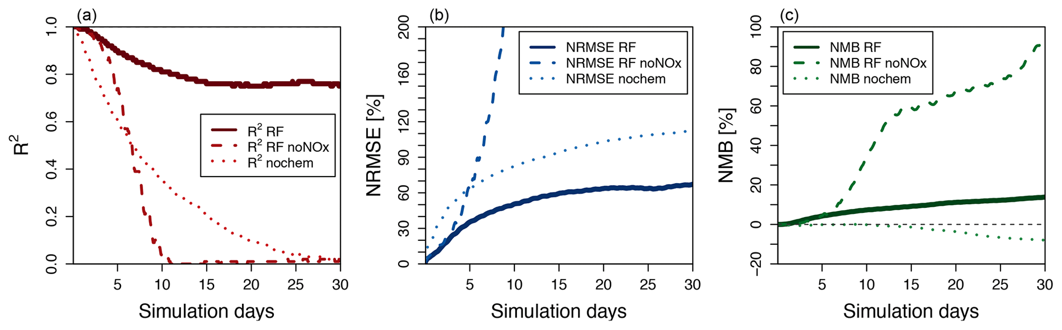
Figure 6Thirty-day evolution of R2 (a), NRMSE (b) and NMB (c) for three different model simulations of O3 run for July 2014 compared to the full GEOS-Chem simulation. The solid line represents the standard random forest (RF) simulation using the family prediction of NOx. The dashed line uses RF predictors for NO and NO2 individually (this simulation becomes unstable after 23 days). The dotted line represents a simulation with no chemistry. The grey line in (c) indicates a 0 value.
Although there are some obvious issues associated with the RFR simulation, it is evident that for many applications, the model has sufficient fidelity to be useful. We now focus on the model's ability to simulate surface O3 and NO2, two important air pollutants.
3.2 Surface concentrations of O3 and NOx
Figure 7 compares concentration maps of surface O3 at 00:00 UTC calculated by the full-chemistry model (upper row), the RFR model (middle row) and their ratio (bottom row) after 1, 5, 10 and 30 days of simulation. After 1 day there are only small differences between the full model and the RFR model. However, these differences grow over the period of the simulation as errors accumulate. By the time the model has been run for 10 days, the model has become significantly biased over clean background regions, in particular over the Pacific Ocean. The differences between the reference model and the RFR simulation grow more slowly after 10 days (see also Fig. 6), resulting in the model differences between day 10 and day 30 being small relative to the difference between day 1 and day 10. It appears that the RFR model finds a new “chemical equilibrium” for surface O3 on the timescale of a few days. This new equilibrium overestimates O3 in clean background regions such as the tropical Pacific and underestimates O3 in the Arctic.
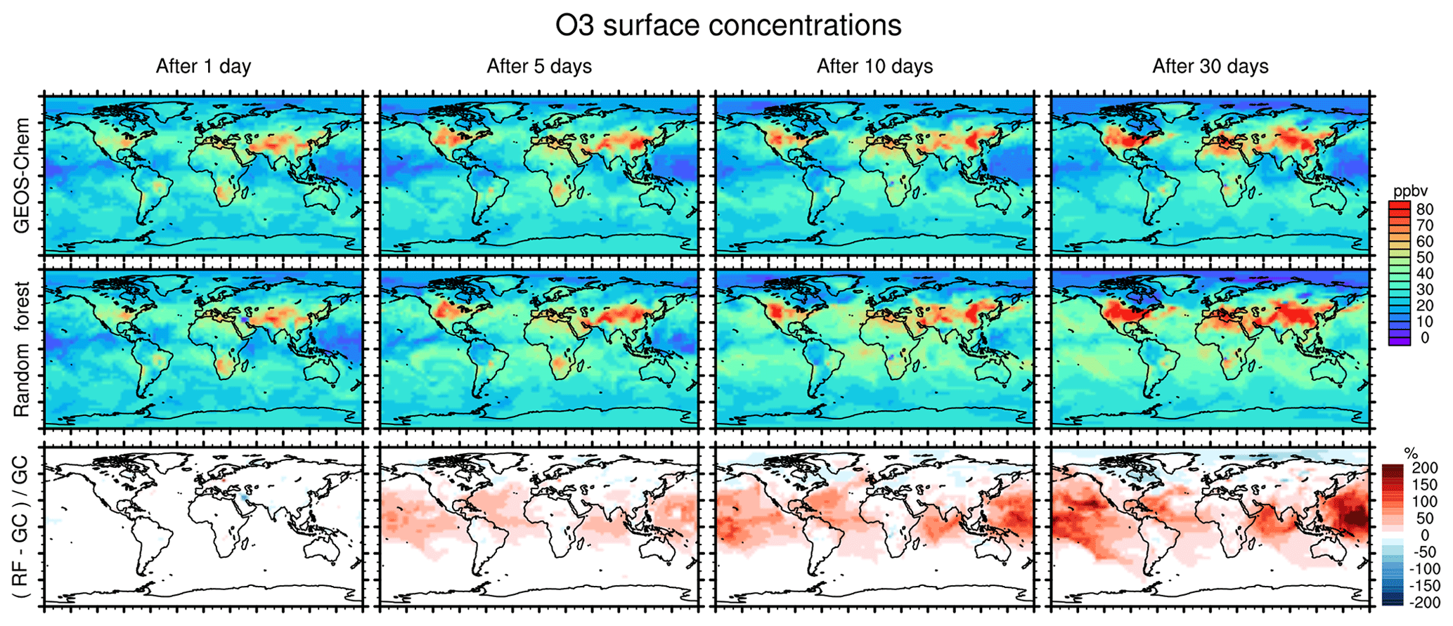
Figure 7Concentration maps of surface O3 mixing ratio after 1 simulation day (column 1), 5 simulation days (column 2), 10 simulation days (column 3) and 30 simulation days (column 4), as calculated by the full GEOS-Chem model (row 1) and the standard random forest (RF) model with the NOx family treatment (row 2). Row 3 shows the percentage difference between the RF simulation and GEOS-Chem (GC).
Figure 8 similarly compares concentration maps of surface NOx. Reflecting the shorter lifetime of NOx, the errors here grow more quickly compared to O3 but level off after 5 days as a new chemical equilibrium is reached. The RFR model shows large differences compared to the GEOS-Chem model in regions where NOx concentrations are low and remote from recent emission, with NOx being highly overestimated in the tropics and underestimated at the poles. This pattern is highly consistent with the ones seen for O3, suggesting that the relative change in NOx drives the change in O3, as would also be the case in a full-chemistry model.
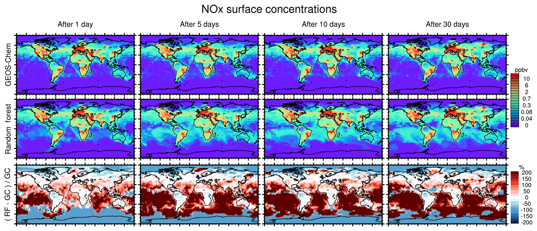
Figure 8Concentration maps of surface NOx (NO + NO2) after 1 simulation day (column 1), 5 simulation days (column 2), 10 simulation days (column 3) and 30 simulation days (column 4), as calculated by the full GEOS-Chem model (row 1) and the standard random forest (RF) model with the NOx family treatment (row 2). Row 3 shows the percentage difference between the RF simulation and GEOS-Chem (GC).
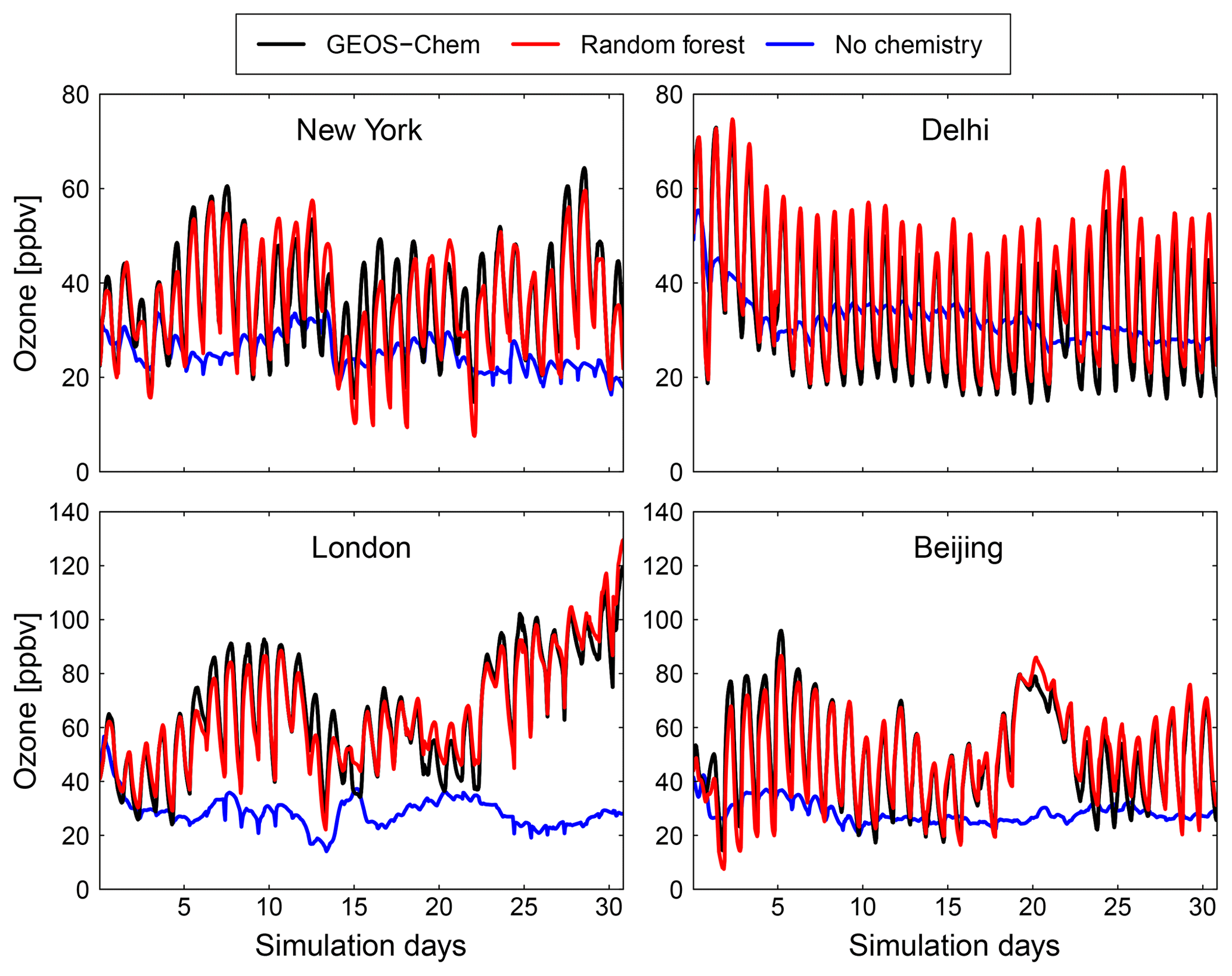
Figure 9Comparison of surface concentration of O3 at four locations (New York, Delhi, London and Beijing) for the GEOS-Chem reference simulation (black), the RFR model with the NO3 family treatment (red) and a simulation with no chemistry (blue).
Figures 9 and 10 show time series of O3 and NOx mixing ratios at four polluted locations (New York, Delhi, London and Beijing) as generated by the full-chemistry model (black line), the RFR model (red), and the model with no chemistry (blue). The RFR model closely follows the full model at these locations and captures the concentrations patterns with an accuracy of 10 %–20 %. Especially for NOx it is hard to distinguish the RFR model from the full model, whereas the simulation without any chemistry shows a distinctly different pattern. These differences are significantly less than one would expect from running two different chemistry models for the same period (e.g. Stevenson et al., 2006; Cooper et al., 2014; Young et al., 2018; Brasseur et al., 2018). Events such as that in Beijing on day 20 are well simulated by the RFR model, which is able to follow the full model, whereas the simulation without chemistry follows a distinctly different path that is solely determined by the net effects of emission, deposition and (vertical and horizontal) transport.
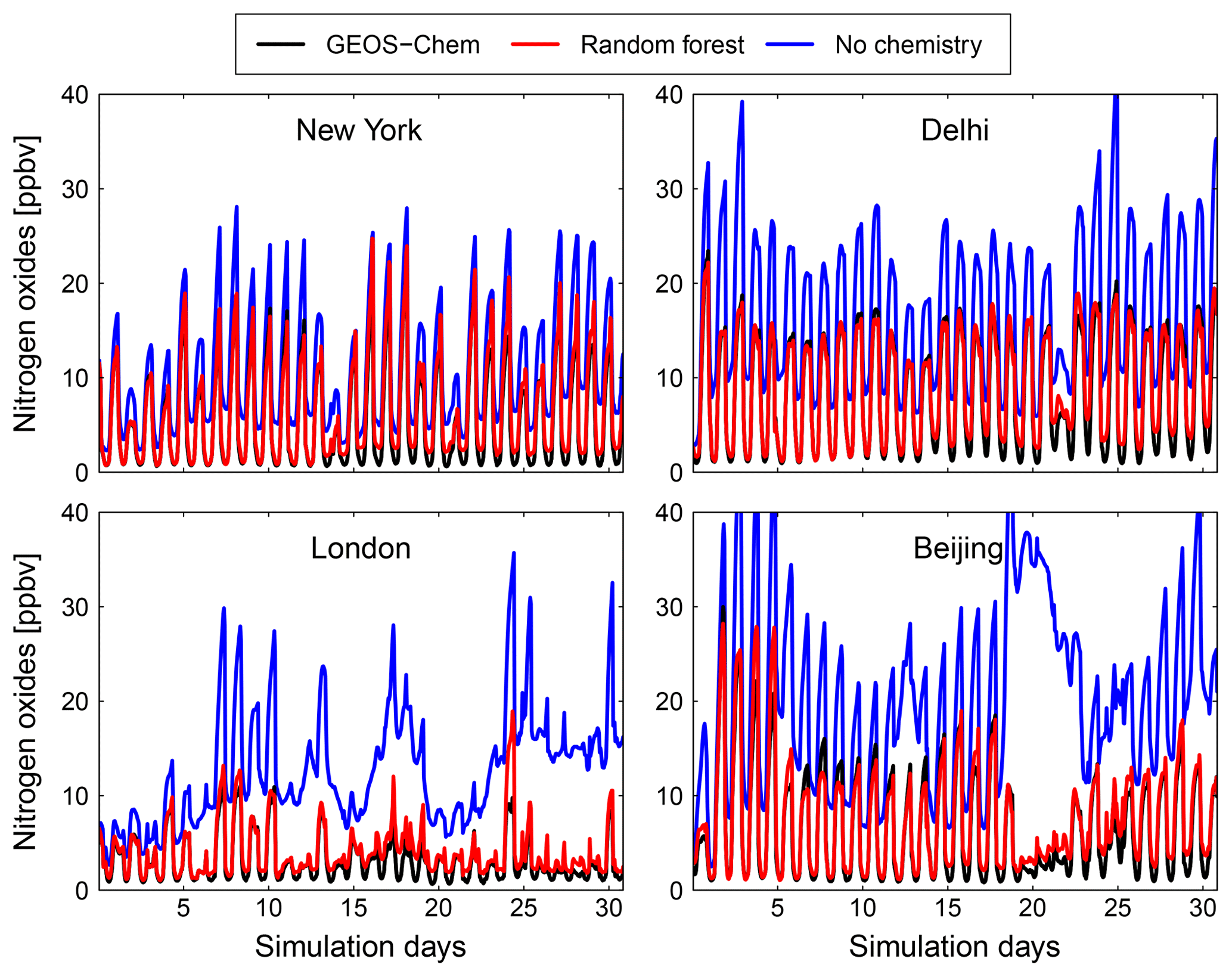
Figure 10Comparison of surface concentration of nitrogen oxides (NOx = NO + NO2) at four locations (New York, Delhi, London and Beijing) for the GEOS-Chem reference simulation (black), the RFR model with the NO3 family treatment (red) and a simulation with no chemistry (blue).
Although our analysis has not provided a complete analysis of the RFR model performance, we have shown that it is capable of providing a simulation of many key facets of the atmospheric chemistry system (O3, NOx) on the timescale of days to weeks. We now discuss future routes to improve the system and some applications.
We have shown that a machine learning algorithm, here random forest regression, can simulate the general features of the chemical integrator used to represent the chemistry scheme in an atmospheric chemistry model. This represents the first stage in producing a fully practical methodology. Here we discuss some of the issues we have found with our approach, potential solutions, some limitations and where we think a machine learning model could provide useful applications.
4.1 Speed, algorithms and hardware
The current RFR implementation takes about twice as long to solve the chemistry as the currently implemented integrator approach. While the evaluation of a single tree is fast (average execution time is ms on the Discover computer system), calculating them all for every forest and for every transported species (30×51) in series results in a total average execution time of 2.6 ms, which is 85 % slower than the average execution time of 1.4 ms using the standard model integrator.
We emphasize that this implementation is a proof of concept. Unlike for the chemical integrator, little work has been undertaken to optimize the algorithm parameters (e.g. optimizing the number of trees or the number of leaves per tree) or the Fortran90 implementation of the forests. For example, random forest have relatively large memory footprints that scale linearly with number of forests and trees. Efficient access of these data through optimal co-location of related information (e.g. grouping memory by branches) could dramatically reduce CPU register loading costs, as could moving from double precision to single precision or even integer maths. In the current implementation, we load all tree data onto every CPU separately without attempts of memory sharing. Thus we believe that different software structures, algorithms and memory management may allow significant increases in the speed achieved.
A fundamental attractiveness of the random forest algorithm is its almost perfect parallel nature, even among species within the same grid cell: the nodes of all trees (and across all forests) solely depend on the initial values of the input features and thus can be evaluated independently of one another (in contrast, the system of coupled ODEs solved by the chemical solver requires coupling between the species). This would readily allow for parallelization of the chemistry operator, which has up to this point not been possible. This may allow other hardware paradigms (e.g. graphical processing units) to be exploited in calculating the chemistry.
We have implemented the replacement for the chemical integrator using the random forest regression algorithm. Our choice here was based on the conceptual ease of the algorithm. However, other algorithms are capable of fulfilling the same function. Neural networks have been used extensively in many Earth system applications (e.g. Krasnopolsky et al., 2010; Brenowitz and Bretherton, 2018; Silva and Heald, 2018), and gradient boosting frameworks such as XGBoost (Chen and Guestrin, 2016) are becoming increasingly popular. A number of different algorithms need to be tested and explored for both speed and accuracy before a best-case algorithm can been found.
4.2 Training data
We have trained the random forest regression models on a single month of data. For a more general system the models will need to be trained with a more temporally extensive data set. Models are, however, able to generate large volumes of data. A year's worth of training data over the full extent of the model's atmosphere would result in a potentially very large (2×10¹⁰) training data set. Applying this methodology to spatial scales relevant to air quality applications (on the order of 10 km) will result in even larger data sets (1013). However, not all items from the training data are of equal value. Much of the atmosphere is made up of chemically similar air masses (e.g. central Pacific, remote free troposphere) which are highly represented in the training data but are not very variable. Most of the interest from an air quality perspective lies in small regions of intense chemistry. If a way can be found to reduce the complete training data set such that the sub-sample represents a statistical description of the full data, the amount of training data can be significantly reduced and thus the time needed to train the system.
The features being used to train the predictors could also be reconsidered. The current selection reflects an initial estimate of the appropriate features. It is evident that different and potentially better choices could be made. For example, we have included all photolysis rates, but these correlate very strongly and so a greatly reduced number of photolysis inputs (potentially from a principal components analysis) could achieve the same results but with a reduced number of features. Including other parameters such as the concentrations of the aerosol tracers may also improve the simulation.
4.3 Conservation laws and error checking
One of the fundamental laws of chemistry is the conservation of atoms. One interpretation of that has been applied here to the prediction of the change in NOx together with predictions for NO:NOx. Since the concentration of NOx changes much more slowly than the change in concentration of either NO or NO2, this approach attempts to improve the prediction of these short-lived nitrogen species, which are difficult to predict. Our results show that this does indeed increase the stability of the system, and it represents a first step towards ensuring the conservation of atoms in machine-learning-based chemistry models. A larger nitrogen family (NO, NO2,NO3, N2O5, HONO, HO2NO2, etc.) might increase stability further, as could other chemical families such as BrOx, which showed significant errors both compared to the validation data and the evaluation of the chemistry model.
The solution space of a chemistry model is constrained by mass-balance requirements, and chemical concentrations tend to mean-revert to the equilibrium concentration implied by the chemical boundary conditions (emissions, deposition rates, sunlight intensity, etc.). A successful machine learning method should have the same qualities in order to prevent runaway errors that can arise from systematic model errors, e.g. if the model constantly over- or under-predicts certain species or if it violates the conservation of mass balance. Because each model prediction feeds into the next one, small errors compound and quickly lead to systematic model errors. Possible solutions for this involve prediction across multiple time steps, which have shown to yield more stable solutions for physical systems (Brenowitz and Bretherton, 2018), or the use of additional constraints that measure the connectivity between chemical species, e.g. through the consideration of the stoichiometric coefficients of all involved reaction rates.
4.4 Possible implementations
The ability to represent the atmospheric chemistry as a set of individual machine learning models (one for each species) rather than as one simultaneous integration has numerous advantages. In locations where the impact of a (relatively short-lived) molecule is known to be insignificant (for example isoprene over the polar regions or dimethyl sulfide (DMS) over the deserts), the differential equation approach continues to solve the chemistry for all species. However, with this machine learning methodology, there would be no need to call the machine learning algorithm for a species with a concentration below a certain threshold or for certain chemical environments (e.g. nighttime): the chemistry could continue without updating the change in the concentration of these species. Thus it would be easy to implement a dynamical chemistry approach which uses a simple lookup table with predefined threshold rates to evaluate whether the concentration of a compound needs to be updated or not. If it did, the machine learning algorithm could be run; if it did not, the concentration would remain untouched and the evaluation of the random forest emulator is skipped (for this species). This approach could reduce the computational burden of atmospheric chemistry yet further.
The machine learning methodology could also be implemented to work seamlessly with the integrator. For example, the full numerical integrator can be used over regions of particular interest (populated areas for an air quality model or a research domain for a research model), while outside of these regions (over the ocean or in the free troposphere for an air quality model or outside of the research domain for a research model) the machine learning could be used. This would provide a “best of both worlds” approach which provides higher chemical accuracy where necessary and faster but lower-accuracy solutions where appropriate.
Our methodology uses the output from the atmospheric chemistry model to generate the training data set. Another approach would be to use a series of box model simulations using initial conditions covering the appropriate chemical concentration ranges to generate the training data. This could allow the chemical complexity that is known to exist (e.g. Aumont et al., 2005; Jenkin et al., 1997) to be encoded in a way which would make it suitable for use in an atmospheric chemistry model. Much of this chemical complexity occurs in relatively small volumes of the atmosphere, for example, urban environments or over forested areas. These are areas with large emissions of complex volatile organic compounds which have a complex degradation chemistry. It would be possible to develop a machine-learning-based chemistry, trained on a number of box model simulations of the complex chemistry, which would represent this chemical complexity in a more efficient form, and to use this machine learning chemistry in only those grid boxes that require the full complex chemistry.
4.5 Limitations
This is the first step in constructing a new methodology for the representation of chemistry in atmospheric models. There are a number of limitations that should be explored in future work. Firstly, the machine learning methodology can only be applied within the range of the data used for the training. Applying the algorithm outside of this range would likely lead to inaccurate results. For example, the model here has been trained for the present-day environment. Although the training data set has seen a range of atmospheric conditions, it has only seen a limited range of methane (CH4) concentrations or temperatures. Thus applying the model to the pre-industrial period or the future, where the CH4 concentration and temperature may be significantly different than in the present day, would likely result in errors. Similarly, exploring scenarios where the emissions into the atmosphere change significantly (for example large changes in NOx emissions vs. VOC emissions) again will likely ask the model to make predictions outside of the range of training data. A simple check would be to evaluate the (surface) NOx∕VOC ratios observed in the new model and compare them against the ranges used in the training: if the ratios in the updated model are significantly different from the training data, the RFR model likely needs to be retrained.
The same limitations also apply to model resolution: due to the non-linear nature of chemistry, the numerical solution of chemical kinetics is resolution-dependent, and a machine learning algorithm may not capture this. Thus, care should be taken when applying these approaches outside of the range of the training data.
4.6 Potential uses
Despite the limitations discussed here, there are a number of potential, exciting applications for this kind of methodologies.
The meteorological community has successfully exploited ensembles of predictions to explore uncertainties in weather forecasting (e.g. Molteni et al., 1996). However, air quality forecasting has not been able to explore this tool due to the computational burden involved. Using a computationally cheap machine learning approach, air quality forecasts based on ensemble predictions could become affordable. Ideally, in such a system the primary ensemble member would include the fully integrated numerical solution of the differential equations, while secondary members use the machine learning emulator. Since air quality forecasts are much more sensitive to boundary conditions (e.g. emissions) than initial conditions, the different machine learning members would be used to capture the sensitivity of the air quality forecast to emission scenarios, changes in dry or wet deposition parameters, uncertainties in the chemical rate constants etc. Data assimilation can be applied to determine the initial state for all models, and then the ensembles could be used for probabilistic air quality forecasting. This application is also less sensitive to long-term numerical instability of the machine learning model as the emulator is only used to produce 5–10 day forecasts, while the initial conditions are anchored to the full-chemistry model for every new forecast.
The data assimilation methodology itself could benefit from a machine learning representation of atmospheric chemistry. Data assimilation is often computationally intense, requiring the calculation of the adjoint of the model or running large numbers of ensemble simulations (Carmichael et al., 2008; Sandu and Chai, 2011; Inness et al., 2015; Bocquet et al., 2015). The ability to run these calculations faster would offer significant advantages.
Another potential application area for machine-learning-based chemistry emulators are chemistry–climate simulations. Unlike air quality applications, which focus on small-scale variations in air pollutants over comparatively short periods of time of days to weeks, chemistry–climate studies require long simulation windows of the order of decades. Because of this, machine learning models used for these applications need to be optimized such that they accurately reproduce the (long-term) response of selected species – e.g. ozone and OH – to key drivers such as temperature, photolysis rates and NOx (Nicely et al., 2017; Nowack et al., 2018). The method presented here could be optimized for such an application by simplifying the problem set, with the model trained to reproduce daily or even monthly averaged species concentrations.
We have shown that a suitably trained machine-learning-based approach can replace the integration step within an atmospheric chemistry model run on the timescale of days to weeks. The application of some chemical intuition, by which we separate long-lived from short-lived species, and a basic application of the conservation of atoms to the NOx family leads to significant improvements in model performance. The machine learning implementation is slower than the current model, but very little optimization and software development has thus far been applied to the code.
Methodologies similar to this may offer the potential to accelerate the calculation of chemistry for some atmospheric chemistry applications such as ensembles of air quality forecasts and data assimilation. Future work on both the algorithm and the methodology is necessary to produce a useful solution, but this first step shows promise.
The GEOS-Chem model output used for training and validation is available in netCDF format via the data repository of the University York (https://doi.org/10.15124/e291fdb4-f035-419c-948e-c8c7c978f8d6, Evans and Keller, 2019). A copy of the random forest training code (written in Python) and the model emulator (Fortran) is available upon request from Christoph Keller. GEOS-Chem (http://geos-chem.org, last access: 18 March 2019) is freely available through an open license (http://acmg.seas.harvard.edu/geos/geos_licensing.html, last access: 18 March 2019). The GEOS-5 global modelling system is available through the NASA Open Source Agreement, Version 1.1, and can be accessed at https://gmao.gsfc.nasa.gov/GEOS_systems/geos5_access.php (last access: 18 March 2019), with further instruction available at https://geos5.org/wiki/index.php?title=GEOS-5_public_AGCM_Documentation_and_Access (last access: 18 March 2019).
MJE and CAK came up with the concept and together wrote the paper. MJE developed the algorithm and CAK implemented it into the GEOS model. Both authors devised the experiments.
The authors declare that they have no conflict of interest.
Christoph A. Keller acknowledges support by the NASA Modeling, Analysis and Prediction (MAP) Program. Resources supporting the model simulations were provided by the NASA Center for Climate Simulation at the Goddard Space Flight Center (https://www.nccs.nasa.gov/services/discover). Mat J. Evans acknowledges support from the UK Natural Environment Research Council from the MAGNIFY and BACCUS grants (NE/M013448/1 and NE/L01291X/1). The authors thank Jiawei Zhuang, Makoto M. Kelp, Christopher W. Tessum, J. Nathan Kutz, and Noah D. Brenowitz for valuable discussion.
This paper was edited by David Topping and reviewed by Johannes Flemming.
Aumont, B., Szopa, S., and Madronich, S.: Modelling the evolution of organic carbon during its gas-phase tropospheric oxidation: development of an explicit model based on a self generating approach, Atmos. Chem. Phys., 5, 2497–2517, https://doi.org/10.5194/acp-5-2497-2005, 2005. a
Bey, I., Jacob, D. J., Yantosca, R. M., Logan, J. A., Field, B. D., Fiore, A. M., Li, Q., Liu, H. Y., Mickley, L. J., and Schultz, M. G.: Global modeling of tropospheric chemistry with assimilated meteorology: Model description and evaluation, J. Geophys. Res.-Atmos., 106, 23073–23095, https://doi.org/10.1029/2001JD000807, 2001. a
Bian, H. and Prather, M. J.: Fast-J2: Accurate Simulation of Stratospheric Photolysis in Global Chemical Models, J. Atmos. Chem., 41, 281–296, https://doi.org/10.1023/A:1014980619462, 2002. a
Blasco, J., Fueyo, N., Dopazo, C., and Ballester, J.: Modelling the Temporal Evolution of a Reduced Combustion Chemical System With an Artificial Neural Network, Combust. Flame, 113, 38–52, https://doi.org/10.1016/S0010-2180(97)00211-3, 1998. a
Bocquet, M., Elbern, H., Eskes, H., Hirtl, M., Žabkar, R., Carmichael, G. R., Flemming, J., Inness, A., Pagowski, M., Pérez Camaño, J. L., Saide, P. E., San Jose, R., Sofiev, M., Vira, J., Baklanov, A., Carnevale, C., Grell, G., and Seigneur, C.: Data assimilation in atmospheric chemistry models: current status and future prospects for coupled chemistry meteorology models, Atmos. Chem. Phys., 15, 5325–5358, https://doi.org/10.5194/acp-15-5325-2015, 2015. a
Brasseur, G. P., Xie, Y., Petersen, A. K., Bouarar, I., Flemming, J., Gauss, M., Jiang, F., Kouznetsov, R., Kranenburg, R., Mijling, B., Peuch, V.-H., Pommier, M., Segers, A., Sofiev, M., Timmermans, R., van der A, R., Walters, S., Xu, J., and Zhou, G.: Ensemble forecasts of air quality in eastern China – Part 1: Model description and implementation of the MarcoPolo–Panda prediction system, version 1, Geosci. Model Dev., 12, 33–67, https://doi.org/10.5194/gmd-12-33-2019, 2019. a
Breiman, L.: Random Forests, Mach. Learn., 45, 5–32, https://doi.org/10.1023/A:1010933404324, 2001. a, b
Brenowitz, N. D. and Bretherton, C. S.: Prognostic Validation of a Neural Network Unified Physics Parameterization, Geophys. Res. Lett., 45, 6289–6298, https://doi.org/10.1029/2018GL078510, 2018. a, b, c
Cariolle, D., Moinat, P., Teyssèdre, H., Giraud, L., Josse, B., and Lefèvre, F.: ASIS v1.0: an adaptive solver for the simulation of atmospheric chemistry, Geosci. Model Dev., 10, 1467–1485, https://doi.org/10.5194/gmd-10-1467-2017, 2017. a
Carmichael, G. R., Sandu, A., Chai, T., Daescu, D. N., Constantinescu, E. M., and Tang, Y.: Predicting air quality: Improvements through advanced methods to integrate models and measurements, J. Comput. Phys., 227, 3540–3571, https://doi.org/10.1016/j.jcp.2007.02.024, 2008. a
Chen, T. and Guestrin, C.: XGBoost: A Scalable Tree Boosting System, ArXiv e-prints, 1603.02754, available at: http://arxiv.org/abs/1603.02754 (last access: 18 March 2019), 2016. a
Cooper, O. R., Parrish, D. D., Ziemke, J., Balashov, N. V., Cupeiro, M., Galbally, I. E., Gilge, S., Horowitz, L., Jensen, N. R., Lamarque, J.-F., Naik, V., Oltmans, S. J., Schwab, J., Shindell, D. T., Thompson, A. M., Thouret, V., Wang, Y., and Zbinden, R. M.: Global distribution and trends of tropospheric ozone: An observation-based review, Elementa, 2, 000 029, https://doi.org/10.12952/journal.elementa.000029, 2014. a
Eastham, S. D., Weisenstein, D. K., and Barrett, S. R.: Development and evaluation of the unified tropospheric–stratospheric chemistry extension (UCX) for the global chemistry-transport model GEOS-Chem, Atmos. Environ., 89, 52–63, https://doi.org/10.1016/j.atmosenv.2014.02.001, 2014. a
Eastham, S. D., Long, M. S., Keller, C. A., Lundgren, E., Yantosca, R. M., Zhuang, J., Li, C., Lee, C. J., Yannetti, M., Auer, B. M., Clune, T. L., Kouatchou, J., Putman, W. M., Thompson, M. A., Trayanov, A. L., Molod, A. M., Martin, R. V., and Jacob, D. J.: GEOS-Chem High Performance (GCHP v11-02c): a next-generation implementation of the GEOS-Chem chemical transport model for massively parallel applications, Geosci. Model Dev., 11, 2941–2953, https://doi.org/10.5194/gmd-11-2941-2018, 2018. a
Evans, M. J. and Keller, C. A.: Dataset associated with Keller and Evans, GMD, 2019, University or York, 28 February 2019, https://doi.org/10.15124/e291fdb4-f035-419c-948e-c8c7c978f8d6, made available under a Creative Commons Attribution (CC BY 4.0) licence at https://pure.york.ac.uk/portal/en/datasets/dataset-associated-with-keller-and-evans-gmd-2019(e291fdb4-f035-419c-948e-c8c7c978f8d6).html last access: 18 March 2019. a
Gentine, P., Pritchard, M., Rasp, S., Reinaudi, G., and Yacalis, G.: Could Machine Learning Break the Convection Parameterization Deadlock?, Geophys. Res. Lett., 45, 5742–5751, https://doi.org/10.1029/2018GL078202, 2018. a
Hu, L., Keller, C. A., Long, M. S., Sherwen, T., Auer, B., Da Silva, A., Nielsen, J. E., Pawson, S., Thompson, M. A., Trayanov, A. L., Travis, K. R., Grange, S. K., Evans, M. J., and Jacob, D. J.: Global simulation of tropospheric chemistry at 12.5 km resolution: performance and evaluation of the GEOS-Chem chemical module (v10-1) within the NASA GEOS Earth system model (GEOS-5 ESM), Geosci. Model Dev., 11, 4603–4620, https://doi.org/10.5194/gmd-11-4603-2018, 2018. a, b
Inness, A., Blechschmidt, A.-M., Bouarar, I., Chabrillat, S., Crepulja, M., Engelen, R. J., Eskes, H., Flemming, J., Gaudel, A., Hendrick, F., Huijnen, V., Jones, L., Kapsomenakis, J., Katragkou, E., Keppens, A., Langerock, B., de Mazière, M., Melas, D., Parrington, M., Peuch, V. H., Razinger, M., Richter, A., Schultz, M. G., Suttie, M., Thouret, V., Vrekoussis, M., Wagner, A., and Zerefos, C.: Data assimilation of satellite-retrieved ozone, carbon monoxide and nitrogen dioxide with ECMWF's Composition-IFS, Atmos. Chem. Phys., 15, 5275–5303, https://doi.org/10.5194/acp-15-5275-2015, 2015. a
Jenkin, M., Watson, L., Utembe, S., and Shallcross, D.: A Common Representative Intermediates (CRI) mechanism for VOC degradation. Part 1: Gas phase mechanism development, Atmos. Environ., 42, 7185–7195, https://doi.org/10.1016/j.atmosenv.2008.07.028, 2008. a
Jenkin, M. E., Saunders, S. M., and Pilling, M. J.: The tropospheric degradation of volatile organic compounds: a protocol for mechanism development, Atmos. Environ., 31, 81–104, https://doi.org/10.1016/S1352-2310(96)00105-7, 1997. a
Jiang, G., Xu, J., and Wei, J.: A Deep Learning Algorithm of Neural Network for the Parameterization of Typhoon–Ocean Feedback in Typhoon Forecast Models, Geophys. Res. Lett., 45, 3706–3716, https://doi.org/10.1002/2018GL077004, 2018. a
Kelp, M. M., Tessum, C. W., and Marshall, J. D.: Orders-of-magnitude speedup in atmospheric chemistry modeling through neural network-based emulation, ArXiv e-prints, 1808.03874, available at: https://arxiv.org/abs/1808.03874 (last access: 18 March 2019), 2018. a
Krasnopolsky, V. M.: Neural network emulations for complex multidimensional geophysical mappings: Applications of neural network techniques to atmospheric and oceanic satellite retrievals and numerical modeling, Rev. Geophys., 45, RG3009, https://doi.org/10.1029/2006RG000200, 2007. a
Krasnopolsky, V. M., Fox-Rabinovitz, M. S., and Chalikov, D. V.: New Approach to Calculation of Atmospheric Model Physics: Accurate and Fast Neural Network Emulation of Longwave Radiation in a Climate Model, Mon. Weather Rev., 133, 1370–1383, https://doi.org/10.1175/MWR2923.1, 2005. a
Krasnopolsky, V. M., Fox-Rabinovitz, M. S., Hou, Y. T., Lord, S. J., and Belochitski, A. A.: Accurate and Fast Neural Network Emulations of Model Radiation for the NCEP Coupled Climate Forecast System: Climate Simulations and Seasonal Predictions, Mon. Weather Rev., 138, 1822–1842, https://doi.org/10.1175/2009MWR3149.1, 2010. a, b
Leighton, P.: Photochemistry of Air Pollution, Academic Press, New York, ISBN 9780323156455, 1961. a
Long, M. S., Yantosca, R., Nielsen, J. E., Keller, C. A., da Silva, A., Sulprizio, M. P., Pawson, S., and Jacob, D. J.: Development of a grid-independent GEOS-Chem chemical transport model (v9-02) as an atmospheric chemistry module for Earth system models, Geosci. Model Dev., 8, 595–602, https://doi.org/10.5194/gmd-8-595-2015, 2015. a, b
Mallet, V., Stoltz, G., and Mauricette, B.: Ozone ensemble forecast with machine learning algorithms, J. Geophys. Res.-Atmos., 114, D05307, https://doi.org/10.1029/2008JD009978, 2009. a
Mao, J., Jacob, D. J., Evans, M. J., Olson, J. R., Ren, X., Brune, W. H., Clair, J. M. St., Crounse, J. D., Spencer, K. M., Beaver, M. R., Wennberg, P. O., Cubison, M. J., Jimenez, J. L., Fried, A., Weibring, P., Walega, J. G., Hall, S. R., Weinheimer, A. J., Cohen, R. C., Chen, G., Crawford, J. H., McNaughton, C., Clarke, A. D., Jaeglé, L., Fisher, J. A., Yantosca, R. M., Le Sager, P., and Carouge, C.: Chemistry of hydrogen oxide radicals (HOx) in the Arctic troposphere in spring, Atmos. Chem. Phys., 10, 5823–5838, https://doi.org/10.5194/acp-10-5823-2010, 2010. a
Mao, J., Paulot, F., Jacob, D. J., Cohen, R. C., Crounse, J. D., Wennberg, P. O., Keller, C. A., Hudman, R. C., Barkley, M. P., and Horowitz, L. W.: Ozone and organic nitrates over the eastern United States: Sensitivity to isoprene chemistry, J. Geophys. Res.-Atmos., 118, 11256–11268, https://doi.org/10.1002/jgrd.50817, 2013. a
Mjolsness, E. and DeCoste, D.: Machine Learning for Science: State of the Art and Future Prospects, Science, 293, 2051–2055, https://doi.org/10.1126/science.293.5537.2051, 2001. a
Molteni, F., Buizza, R., Palmer, T. N., and Petroliagis, T.: The ECMWF Ensemble Prediction System: Methodology and validation, Q. J. Roy. Meteor. Soc., 122, 73–119, https://doi.org/10.1002/qj.49712252905, 1996. a
Murray, L. T., Jacob, D. J., Logan, J. A., Hudman, R. C., and Koshak, W. J.: Optimized regional and interannual variability of lightning in a global chemical transport model constrained by LIS/OTD satellite data, J. Geophys. Res.-Atmos., 117, d20307, https://doi.org/10.1029/2012JD017934, 2012. a
Nicely, J. M., Salawitch, R. J., Canty, T., Anderson, D. C., Arnold, S. R., Chipperfield, M. P., Emmons, L. K., Flemming, J., Huijnen, V., Kinnison, D. E., Lamarque, J.-F., Mao, J., Monks, S. A., Steenrod, S. D., Tilmes, S., and Turquety, S.: Quantifying the causes of differences in tropospheric OH within global models, J. Geophys. Res.-Atmos., 122, 1983–2007, https://doi.org/10.1002/2016JD026239, 2017. a, b
Nielsen, J. E., Pawson, S., Molod, A., Auer, B., da Silva, A. M., Douglass, A. R., Duncan, B., Liang, Q., Manyin, M., Oman, L. D., Putman, W., Strahan, S. E., and Wargan, K.: Chemical Mechanisms and Their Applications in the Goddard Earth Observing System (GEOS) Earth System Model, J. Adv. Model. Earth Sy., 9, 3019–3044, https://doi.org/10.1002/2017MS001011, 2017. a
Nowack, P., Braesicke, P., Haigh, J., Abraham, N. L., Pyle, J., and Voulgarakis, A.: Using machine learning to build temperature-based ozone parameterizations for climate sensitivity simulations, Environ. Res. Lett., 13, 104016, https://doi.org/10.1088/1748-9326/aae2be, 2018. a, b
Parrella, J. P., Jacob, D. J., Liang, Q., Zhang, Y., Mickley, L. J., Miller, B., Evans, M. J., Yang, X., Pyle, J. A., Theys, N., and Van Roozendael, M.: Tropospheric bromine chemistry: implications for present and pre-industrial ozone and mercury, Atmos. Chem. Phys., 12, 6723–6740, https://doi.org/10.5194/acp-12-6723-2012, 2012. a
Pedregosa, F., Varoquaux, G., Gramfort, A., Michel, V., Thirion, B., Grisel, O., Blondel, M., Prettenhofer, P., Weiss, R., Dubourg, V., Vanderplas, J., Passos, A., Cournapeau, D., Brucher, M., Perrot, M., and Duchesnay, E.: Scikit-learn: Machine Learning in Python, J. Mach. Learn. Res., 12, 2825–2830, 2011. a
Porumbel, I., Petcu, A. C., Florean, F. G., and Hritcu, C. E.: Artificial Neural Networks for Modeling of Chemical Source Terms in CFD Simulations of Turbulent Reactive Flows, in: Modeling and Optimization of the Aerospace, Robotics, Mechatronics, Machines-Tools, Mechanical Engineering and Human Motricity Fields, Vol. 555, Applied Mechanics and Materials, Trans Tech Publications, 395–400, 2014. a
Sandu, A. and Chai, T.: Chemical Data Assimilation – An Overview, Atmosphere, 2, 426–463, https://doi.org/10.3390/atmos2030426, 2011. a
Sandu, A. and Sander, R.: Technical note: Simulating chemical systems in Fortran90 and Matlab with the Kinetic PreProcessor KPP-2.1, Atmos. Chem. Phys., 6, 187–195, https://doi.org/10.5194/acp-6-187-2006, 2006. a
Sandu, A., Verwer, J., Blom, J., Spee, E., Carmichael, G., and Potra, F.: Benchmarking stiff ode solvers for atmospheric chemistry problems II: Rosenbrock solvers, Atmos. Environ., 31, 3459–3472, https://doi.org/10.1016/S1352-2310(97)83212-8, 1997a. a
Sandu, A., Verwer, J., Loon, M. V., Carmichael, G., Potra, F., Dabdub, D., and Seinfeld, J.: Benchmarking stiff ode solvers for atmospheric chemistry problems-I. implicit vs explicit, Atmos. Environ., 31, 3151–3166, https://doi.org/10.1016/S1352-2310(97)00059-9, 1997b. a
Santillana, M., Sager, P. L., Jacob, D. J., and Brenner, M. P.: An adaptive reduction algorithm for efficient chemical calculations in global atmospheric chemistry models, Atmos. Environ., 44, 4426–4431, https://doi.org/10.1016/j.atmosenv.2010.07.044, 2010. a
Silva, S. J. and Heald, C. L.: Investigating Dry Deposition of Ozone to Vegetation, J. Geophys. Res.-Atmos., 123, 559–573, https://doi.org/10.1002/2017JD027278, 2018. a
Stevenson, D. S., Dentener, F. J., Schultz, M. G., Ellingsen, K., van Noije, T. P. C., Wild, O., Zeng, G., Amann, M., Atherton, C. S., Bell, N., Bergmann, D. J., Bey, I., Butler, T., Cofala, J., Collins, W. J., Derwent, R. G., Doherty, R. M., Drevet, J., Eskes, H. J., Fiore, A. M., Gauss, M., Hauglustaine, D. A., Horowitz, L. W., Isaksen, I. S. A., Krol, M. C., Lamarque, J.-F., Lawrence, M. G., Montanaro, V., Müller, J.-F., Pitari, G., Prather, M. J., Pyle, J. A., Rast, S., Rodriguez, J. M., Sanderson, M. G., Savage, N. H., Shindell, D. T., Strahan, S. E., Sudo, K., and Szopa, S.: Multimodel ensemble simulations of present-day and near-future tropospheric ozone, J. Geophys. Res.-Atmos., 111, D08301, https://doi.org/10.1029/2005JD006338, 2006. a
Turányi, T.: Parameterization of reaction mechanisms using orthonormal polynomials, Comput. Chem., 18, 45–54, https://doi.org/10.1016/0097-8485(94)80022-7, 1994. a
Whitehouse, L. E., Tomlin, A. S., and Pilling, M. J.: Systematic reduction of complex tropospheric chemical mechanisms, Part I: sensitivity and time-scale analyses, Atmos. Chem. Phys., 4, 2025–2056, https://doi.org/10.5194/acp-4-2025-2004, 2004a. a
Whitehouse, L. E., Tomlin, A. S., and Pilling, M. J.: Systematic reduction of complex tropospheric chemical mechanisms, Part II: Lumping using a time-scale based approach, Atmos. Chem. Phys., 4, 2057–2081, https://doi.org/10.5194/acp-4-2057-2004, 2004b. a
Young, P. J., Naik, V., Fiore, A. M., Gaudel, A., Guo, J., Lin, M. Y., Neu, J. L., Parrish, D. D., Rieder, H. E., Schnell, J. L., Tilmes, S., Wild, O., Zhang, L., Ziemke, J. R., Brandt, J., Delcloo, A., Doherty, R. M., Geels, C., Hegglin, M. I., Hu, L., Im, U., Kumar, R., Luhar, A., Murray, L., Plummer, D., Rodriguez, J., Saiz-Lopez, A., Schultz, M. G., Woodhouse, M. T., and Zeng, G.: Tropospheric Ozone Assessment Report: Assessment of global-scale model performance for global and regional ozone distributions, variability, and trends, Elementa, 6, 10, https://doi.org/10.1525/elementa.265, 2018. a
Young, T. R. and Boris, J. P.: A numerical technique for solving stiff ordinary differential equations associated with the chemical kinetics of reactive-flow problems, J. Phys. Chem., 81, 2424–2427, https://doi.org/10.1021/j100540a018, 1977. a