Meso-NH-ISO v1.0: a water stable isotopologue scheme in the non-hydrostatic mesoscale atmospheric model Meso-NH – application to a 2D West African squall line

Better understanding how convective processes impact the isotopic composition of atmospheric water has implications for understanding phenomena such as squall lines or tropical cyclones, and for reconstructions of past rainfall extreme events. With this motivation, we implemented water stable isotopologues (HD¹⁶O and H${}_{\mathrm{2}}^{\mathrm{18}}$O) in the non-hydrostatic mesoscale atmospheric model Meso-NH and its one-moment bulk mixed-phase microphysics scheme. The water stable isotopologues are subject to the same dynamical and physical processes as the light water, but undergo isotopic fractionation during water phase changes. Both equilibrium and kinetic fractionation processes that occur during water phase changes involving water vapor are taken into account. The implementation is validated on a test case of a 2D simulation of a tropical squall line observed in June 1981 during the COPT 81 field campaign in the Sahel region. The isotopic version of Meso-NH (Meso-NH-ISO) captures the expected evolution of the isotopic composition of both precipitation and water vapor along the squall line. This work opens the door to future isotopic studies using realistic cases of mesoscale convective systems (squall lines, tropical cyclones).

1 Introduction

The isotopic composition of water vapor and precipitation (deuterium and oxygen-18) is a useful tool to better understand convective processes in the present-day water cycle, such as the contribution of rainfall evaporation to the moistening of the lower troposphere (Worden et al., 2007) or the contribution of convective detrainment and sublimation of ice crystals to the moistening of the upper troposphere and lower stratosphere (Moyer et al., 1996; Webster and Heymsfield, 2003; Hanisco et al., 2007).

The isotopic composition of precipitation recorded in climate archives has also significantly contributed to the reconstruction of past changes in precipitation in tropical regions (Wang et al., 2001; Cruz et al., 2009). This is based on the observation that precipitation is more depleted when precipitation rate is larger, called the amount effect (Dansgaard, 1964). Convective processes, such as convective downdraft, mesoscale descent, rain evaporation below cloud, and rain melt under stratiform clouds, contribute to the amount effect (Worden et al., 2007; Risi et al., 2008a; Kurita, 2013; Risi et al., 2021). Since these processes are expected to vary with the organization and characteristics of tropical convection, the water isotopic composition also depends on the proportion of stratiform versus convective rain (Aggarwal et al., 2016), on the mesoscale organization of convection (Lawrence et al., 2004; Risi et al., 2008b; Chakraborty et al., 2016; Vimeux et al., 2024) or on the convective depth (Moore et al., 2014; Torri et al., 2017; Lacour et al., 2017).

All these applications of water stable isotopologues observations require a better understanding of how convective processes impact the isotopic composition of water vapor and precipitation. A large number of modeling studies have relied on models with parameterized convection (e.g. Lee et al., 2007; Bony et al., 2008), but these models are limited by the shortcomings and uncertainties associated with the parameterization of convection (Randall et al., 2003; Webb et al., 2015). To explicitly resolve convective motions, we need models that resolve the non-hydrostatic equations of motion at a resolution of the order of the kilometer or finer, such as cloud-resolving models or large-eddy simulation models. Several such models have been implemented with water stable isotopes in the past few years. The DHARMA cloud model integrates the evolution of HD¹⁶O within a bin microphysics scheme explicitly representing cloud condensation nuclei, water droplets, and ice crystals using 16 mass bins, as described by Smith et al. (2006). The 2-moment bin mixed-phase microphysics scheme DESCAM has recently been extended to simulate the evolution of oxygen-18 within a 1.5D dynamical framework (Hiron and Flossmann, 2020). Such bin microphysics schemes are undoubtedly an advantage for accounting for different isotopic compositions depending on particle size, but it comes at a very high computational cost. Thus, DHARMA and DESCAM typically track only one water stable isotopologue in addition to light water species. On the other hand, numerical models employing bulk microphysics schemes usually simulate the evolution of both HD¹⁶O and H${}_{\mathrm{2}}^{\mathrm{18}}$O. This includes models such as SAM-ISO (Blossey et al., 2010), COSMO-ISO (Pfahl et al., 2012), WRF-ISO (Moore et al., 2016), and, more recently, NICAM-WISO (Tanoue et al., 2023). All these models incorporate the evolution of the two isotopologues into a bulk microphysics scheme. The microphysics schemes in SAM-ISO, WRF-ISO, and NICAM-WISO typically describe the evolution of water vapor, cloud water, rain, cloud ice, snow, and graupel mass. However, graupel is not considered in COSMO-ISO.

Here, we implemented water stable isotopologues in the non-hydrostatic atmospheric model Meso-NH (Lac et al., 2018). This model is flexible enough to be used for idealized simulations, realistic case studies or global simulations, and can deal with scales ranging from synoptic to large eddy scales. In the past few years, it has taken part in various model intercomparison projects, such as RCEMIP (Wing et al., 2018) or DYAMOND (Stevens et al., 2019). Its physical package can also be shared with the LMDZ general circulation model (Hourdin et al., 2020) and can be used in the non-hydrostatic version of the icosahedral DYNAMICO model (Dubos et al., 2015). Our ultimate goal is to simulate realistic case studies with various mesoscale convective systems, including tropical cyclones and squall lines. In the meanwhile, a first step is to implement water stable isotopologues in Meso-NH. The goal of this article is to describe this implementation, and to validate it on a simple case. The Meso-NH model and its one-moment microphysical scheme are shortly described in the first section. The second section is dedicated to the description of the newly implemented water isotope scheme in Meso-NH. In a third section, first results from a 2D simulation of a Sahelian squall line observed during the COPT 81 field campaign are presented.

2 The Meso-NH model

The water stable isotopologues scheme described in Sect. 3 is implemented in version 5-5-0 of the Meso-NH model, and is coupled to the one-moment bulk microphysics scheme (ICE3, Pinty and Jabouille, 1998).

2.1 Short overview of Meso-NH

Meso-NH is a non-hydrostatic mesoscale atmospheric model (Lac et al., 2018). It enables simulating atmospheric phenomena from the small-scale (down to a few meters) to the synoptic-scale (up to several tens of kilometers). A large set of physical parameterizations are available for convection (Bechtold et al., 2001; Pergaud et al., 2009), cloud microphysics (Pinty and Jabouille, 1998; Cohard and Pinty, 2000; Vié et al., 2016; Taufour et al., 2024), turbulence (Cuxart et al., 2000), aerosols (Tulet et al., 2005, 2006), and radiation (Morcrette, 1991; Mlawer et al., 1997; Hogan and Bozzo, 2018). Meso-NH can be coupled with the surface modeling platform SurfEx (Masson et al., 2013) that accounts for natural land surface, urbanized areas, lakes, and oceans. Thus, Meso-NH offers a perfect setting for any simulation of physico-chemical processes in the atmosphere. The reader is referred to Lac et al. (2018) for a more complete description of Meso-NH capabilities for a range of Earth system prediction applications.

2.2 The ICE3 microphysics scheme

ICE3 is a bulk mixed-phase one-moment microphysics scheme (Caniaux et al., 1994; Pinty and Jabouille, 1998) that predicts the mass mixing ratio r of six water species (water vapor, cloud water, raindrops, primary ice crystals, snow aggregates, and graupel). For any species, the mixing ratio is the mass of the species divided by the reference mass of dry air ρ_a.

For cloud droplets, the total number concentrations (N_c) is fixed at 300×10⁶ m⁻³ over land and 100×10⁶ m⁻³ over oceans. For pristine ice, the total number concentration N_i is diagnosed based on the Meyers et al. (1992) parameterization of heterogeneous nucleation. The concentration of the precipitating particles (raindrops, snow/aggregates and graupel) is parameterized according to Caniaux et al. (1994), with the total number concentration given by N=Cλ^x. C and x are empirical constants deduced from observations (see Table 1). λ is the slope parameter of the particle size distribution. In ICE3, the particle size distribution is assumed to follow a generalized Gamma distribution:

$$\begin{array}{}\text{(1)}& n\left(D\right)=Ng\left(D\right)=N{\displaystyle \frac{\mathit{\alpha }}{\mathrm{\Gamma }\left(\mathit{\nu }\right)}}(\mathit{\lambda }D{)}^{\mathit{\alpha }\mathit{\nu }}{D}^{-\mathrm{1}}{e}^{-(\mathit{\lambda }D{)}^{\mathit{\alpha }}}\end{array}$$

where D is the diameter of the particle, g(D) the normalized generalized Gamma distribution and Γ() the Gamma function. α and ν are free shape parameters; their values are given in Table 1. The pth moment of the law writes:

$$\begin{array}{}\text{(2)}& M\left(p\right)=\underset{\mathrm{0}}{\overset{\mathrm{\infty }}{\int }}{D}^{p}g\left(D\right)\mathrm{d}D={\displaystyle \frac{\mathrm{1}}{{\mathit{\lambda }}^p}}{\displaystyle \frac{\mathrm{\Gamma }(\mathit{\nu }+p/\mathit{\alpha })}{\mathrm{\Gamma }\left(\mathit{\nu }\right)}}.\end{array}$$

Table 1 Set of parameters used to characterize each hydrometeor category in the ICE3 microphysics scheme

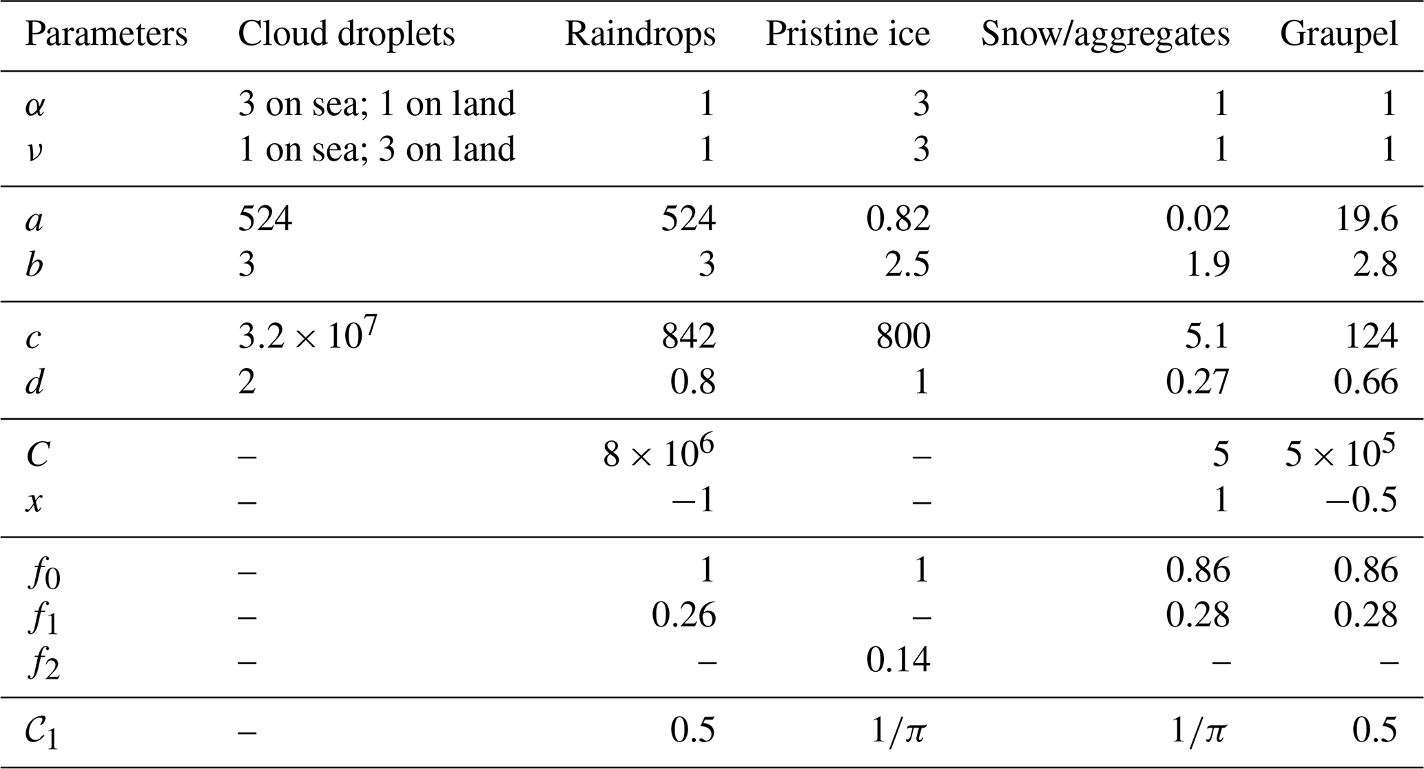
It is also assumed that the mass (m) and terminal fall speed (v) of hydrometeors are related to the particle diameter D following power laws:

$$\begin{array}{}\text{(3)}& m\left(D\right)=a{D}^b\end{array}$$

and

$$\begin{array}{}\text{(4)}& v\left(D\right)=c{D}^d{\left({\displaystyle \frac{{\mathit{\rho }}_{\mathrm{0}}}{{\mathit{\rho }}_{\text{a}}}}\right)}^{\mathrm{0.4}}\end{array}$$

where a, b, c and d are constants given in Table 1. ρ₀ is the reference air density at the surface. Then the mixing ratio is defined by:

$$\begin{array}{}\text{(5)}& r=\underset{\mathrm{0}}{\overset{+\mathrm{\infty }}{\int }}m\left(D\right)n\left(D\right)\mathrm{d}D=aNM\left(b\right)\end{array}$$

while the slope parameter of the particle size distribution writes:

$$\begin{array}{}\text{(6)}& \mathit{\lambda }={\left({\displaystyle \frac{{\mathit{\rho }}_{\text{a}}r\mathrm{\Gamma }\left(\mathit{\nu }\right)}{aN\mathrm{\Gamma }(\mathit{\nu }+b/\mathit{\alpha })}}\right)}^{-\mathrm{1}/b}.\end{array}$$

Each type of hydrometeor has one or more initiation and growth processes as shown in Fig. 1. Warm-phase processes are based on the Kessler (1969) scheme. Raindrops are formed by autoconversion of cloud droplets (AUT), grow through accretion of cloud droplets (ACC), and can evaporate (EVA). Pristine ice crystals are initiated through heterogeneous nucleation (HEN) or by homogeneous nucleation (HON) when the temperature is below −35 °C. These ice crystals grow by deposition (DEP) and through the Bergeron-Findeisen process (BER). Snow/aggregates are formed by autoconversion of pristine ice crystals (AUT), then grow by aggregation of ice crystals (AGG) and by light riming due to collection of cloud droplets (RIM) or to accretion of raindrops (ACC). Then graupel are formed by heavy riming of snow (RIM and ACC) or by contact freezing of ice crystals on raindrops (CFR). They further grow by dry and wet growth mode (DRY, WET). Snow/aggregates and graupel can grow or ablate by water vapor deposition (DEP) or sublimation (SUB). When the temperature drops below 0 °C, ice crystals are immediately transformed into cloud droplets (MLT). Snow/aggregates are converted progressively into graupel particles that melt while falling. The fast vapor exchanges with cloud droplets (CND/EVA) and pristine ice crystals (DEP/SUB) are treated using an implicit adjustment scheme.

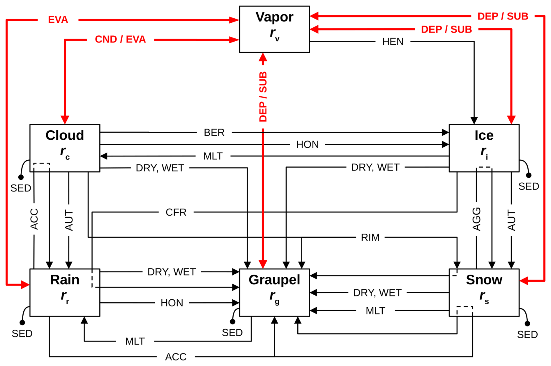
Figure 1 Diagram of the microphysical processes of ICE3. Red arrows show processes involving isotopic fractionation.

The time-step dependency in the original ICE3 scheme is suppressed according to Riette (2020). To eliminate time-step dependency, key modifications include integration of heat budgets to constrain physical processes (e.g., melting) and to fix flawed calculations (e.g., snow-to-graupel conversion). Other adjustments include graupel growth modes (dry/wet), continuous cloud droplet shedding, and symmetric hail/graupel processes, reducing time-step biases. For large time steps (>10 s), time-splitting enables more frequent process interactions. These changes significantly reduce time-step dependency with a modest computational overhead (see Appendix B in Riette, 2020).

3 Formulation of water stable isotopologues in Meso-NH-ISO

3.1 Water stable isotopologues variables

The introduction of water isotopologues into Meso-NH was achieved using a similar approach to previous studies in the development of isotopic models (e.g. Blossey et al., 2010). Analogously, the original water prognostic variables in the model are taken to represent the most common standard light water, H${}_{\mathrm{2}}^{\mathrm{16}}$O. To integrate heavy isotopes in Meso-NH, prognostic variables and equations describing the water cycle of each isotopologue are introduced into the model. As for light water, the mass mixing ratio of each heavy water isotopologue (r^iso) for each water species is a prognostic variable of the model. In practice, each water variable for light molecule H${}_{\mathrm{2}}^{\mathrm{16}}$O is duplicated for heavy molecules HD¹⁶O and H${}_{\mathrm{2}}^{\mathrm{18}}$O. Therefore 12 additional variables are tracked in the model. These additional variables are subject to the same physical processes as the light water variables, and evolve according to:

$$\begin{array}{}\text{(7)}& {\displaystyle \frac{\partial }{\partial t}}\left({\mathit{\rho }}_{\text{a}}{r}^{\mathrm{iso}}\right)+\mathbf{\nabla }\cdot \left({\mathit{\rho }}_{\text{a}}{r}^{\mathrm{iso}}\mathit{U}\right)={\mathit{\rho }}_{\text{a}}{S}^{\mathrm{iso}}\end{array}$$

where U is the 3D air velocity. The source term S^iso includes the turbulent diffusion, the sedimentation by gravity, the microphysical evolution of the particles, and their isotopic fractionation if any. The equations for the source term are given in Sect. 3.2 for non-fractionating processes, and in Sect. 3.3 for fractionating processes. The introduction of water isotopologues in Meso-NH does not interfere with any of the model physics or dynamics. We checked that the model results before and after the introduction of isotopologues are exactly the same.

During the post-processing of model outputs, several diagnostics are computed. The water content in heavy isotopes (HD¹⁶O or H${}_{\mathrm{2}}^{\mathrm{18}}$O) is expressed as:

$$\begin{array}{}\text{(8)}& \mathit{\delta }=\left[{\displaystyle \frac{R}{R_{\mathrm{VSMOW}}}}-\mathrm{1}\right]\end{array}$$

where R stands for either R_D or $R_{{}^{\mathrm{18}}\text{O}}$, and VSMOW is the Vienna Standard Mean Ocean Water. R_D and $R_{{}^{\mathrm{18}}\text{O}}$ are defined as the ratio of deuterium over hydrogen atoms and of ¹⁸O over ¹⁶O atoms in the water, respectively. The isotope ratio R is thus defined for each water species as $r^{\text{iso}}/r$. Although δ is dimensionless, in what follows, δ from Eq. (8) is multiplied by 1000 to express it in ‰, the common unit.

To first order, δD variations in water phases are 8 times those in δ¹⁸O (Craig, 1961). However, slight deviations in δD−δ¹⁸O slopes occur and are mainly due to kinetic effects such as evaporative effects. The later can be quantified by deuterium excess (d-excess) defined as follows (Dansgaard, 1964):

$$\begin{array}{}\text{(9)}& d\text{-excess}=\mathit{\delta }\mathrm{D}-\mathrm{8}\times {\mathit{\delta }}^{\mathrm{18}}\mathrm{O}.\end{array}$$

It is computed for each hydrometeor, and reflects the diffusivity differences between H${}_{\mathrm{2}}^{\mathrm{18}}$O and HD¹⁶O. As a result, when rain evaporation takes place deuterium excess in precipitation decreases.

3.2 Non-fractionating processes

The mass exchange of heavy isotopes during microphysical processes not involving isotopic fractionation is proportional to their relative mass mixing ratio in the reservoir from which the flux comes from. Thus, for each microphysical process without isotopic fractionation, the mass transfer rate for heavy water (Δr^iso) is proportional to the mass transfer rate calculated for standard water provided by the microphysics scheme (Δr). For example, during the accretion of cloud droplets by snow (ACC), the mass mixing ratio transfer rate for HD¹⁶O and H${}_{\mathrm{2}}^{\mathrm{18}}$O writes:

$$\begin{array}{}\text{(10)}& {\left.\mathrm{\Delta }{r}^{\mathrm{iso}}\right|}_{\mathrm{ACC}}={\left.\mathrm{\Delta }r\right|}_{\mathrm{ACC}}\times {\displaystyle \frac{r^{\mathrm{iso}}}{r}}.\end{array}$$

Microphysical processes that do not involve any phase changes do not fractionate, such as processes converting cloud droplets to rain (autoconversion of cloud droplets AUT, growth of raindrops by accretion of cloud droplets ACC) or ice crystals to snow (autoconversion of ice crystals to snow AUT, growth of snow by aggregation of ice crystals AGG). Some microphysical processes involving phase changes are also assumed not to fractionate. For example, when cloud ice melts into cloud droplets (MLT), we assume total melt of each ice crystal, so that there is no fractionation. The same rationale applies for all processes between snow, rain and graupel (MLT, RIM, HON).

Concerning the Bergeron process (BER), we assume it does not fractionate. The Bergeron process is the evaporation of cloud droplets followed by the ice deposition in mixed-phase clouds, when the air is subsaturated with respect to liquid and supersaturated with respect to ice. Since ice deposition in supersaturated conditions is associated with kinetic fractionation, the Bergeron process is often assumed to fractionate (Ciais and Jouzel, 1994). When the Bergeron process is at play in convective updrafts, it acts to enrich the vapor and decrease its d-excess at altitudes above the 0 °C isotherm (Bolot et al., 2013). In ICE3, the mass transfer rate from cloud droplets to ice crystals is assumed to equal the water vapor deposition rate onto pristine ice crystals, which in turn equals the cloud droplets' evaporation rate. This keeps the water vapor reservoir neutral. Therefore, we ignore fractionation during the Bergeron process, as in Blossey et al. (2010). Due to this assumption, we may slightly overestimate the isotopic depletion and the d-excess in the upper troposphere. This is not an issue for science applications focusing on surface precipitation or low-level water vapor, but future refinements might be required for applications in the upper-troposphere.

3.3 Fractionating processes

Isotopic fractionation occurs due to differences in mass and symmetry between the different water molecules. Molecular mass differences induce equilibrium fractionation. Due to a lower saturation vapor pressure for heavy isotopes, the heavier molecules concentrate in the condensed phase. Additionally, kinetic fractionation is induced by diffusivity differences, with a lower diffusivity of heavy isotopes. Then, in order to provide a comprehensive understanding of the distribution of isotopes in water and of the related physical processes, it is necessary to take into account both equilibrium and kinetic fractionation processes that occur during water phase changes.

The following sections explain how isotope fractionation processes are incorporated into Meso-NH. Logic variables controlling the code segments of the model that account for isotopic fractionation can be enabled or disabled to simplify sensitivity analysis, as used by Arnault et al. (2021).

3.3.1 Condensation and evaporation of cloud water

In the ICE3 microphysics scheme, as in most one-moment bulk microphysics scheme, the parameterization of the condensation/evaporation processes consists of a saturation adjustment aimed at restoring the thermodynamic equilibrium between water vapor and cloud droplets. Since the equilibration time for small droplets is normally of the order of seconds, an equilibrium approach may also be used for heavy isotopes (Blossey et al., 2010). Thus, the isotopic fractionation that occurs during droplet condensation within the cloud is considered to be at equilibrium (Bony et al., 2008; Blossey et al., 2010; Arnault et al., 2021), and the differences in molecular diffusivity between the molecules are not taken into account.

At equilibrium:

$$\begin{array}{}\text{(11)}& R_{\text{c}}={\mathit{\alpha }}_{\text{l}/\text{v}}\times R_{\text{w}}\end{array}$$

where R_c and R_w are the isotopic composition of cloud droplets and water vapor, respectively, and ${\mathit{\alpha }}_{\text{l}/\text{v}}$ is the isotopic equilibrium fractionation factor over liquid. Then if the water variables are advanced by one model time step:

$$\begin{array}{}\text{(12)}& {\displaystyle \frac{r_{\text{c}}^{\text{iso}}+{\left.\mathrm{\Delta }{r}^{\text{iso}}\right|}_{\text{CND/EVA}}}{r_{\text{c}}+{\left.\mathrm{\Delta }r\right|}_{\text{CND/EVA}}}}={\mathit{\alpha }}_{\text{l}/\text{v}}\times {\displaystyle \frac{r_{\text{v}}^{\text{iso}}-{\left.\mathrm{\Delta }{r}^{\text{iso}}\right|}_{\text{CND/EVA}}}{r_{\text{v}}-{\left.\mathrm{\Delta }r\right|}_{\text{CND/EVA}}}}.\end{array}$$

Given $B=\frac{r_{\text{c}}+{\left.\mathrm{\Delta }r\right|}_{\text{CND/EVA}}}{r_{\text{v}}-{\left.\mathrm{\Delta }r\right|}_{\text{CND/EVA}}}$, Eq. (12) leads to:

$$\begin{array}{}\text{(13)}& {\left.\mathrm{\Delta }{r}^{\text{iso}}\right|}_{\text{CND/EVA}}={\displaystyle \frac{{\mathit{\alpha }}_{\text{l}/\text{v}}{r}_{\text{v}}^{\text{iso}}B-r_{\text{c}}^{\text{iso}}}{\mathrm{1}+{\mathit{\alpha }}_{\text{l}/\text{v}}B}}.\end{array}$$

Cloud droplets evaporation is also treated in Eq. (13) when Δr|_CND/EVA is negative; it is also assumed to be at equilibrium.

3.3.2 Rain evaporation

For raindrops, due to their larger size, the isotopic equilibrium assumption is not valid, and the mass transfer between the drop and the surrounding vapor must be modeled explicitly. In Meso-NH, the evaporation rate of a raindrop is derived following Pruppacher and Klett (1997) and Seinfeld and Pandis (2016), and the rate of change of a raindrop mass (m_r) finally writes

$$\begin{array}{}\text{(14)}& {\left.{\displaystyle \frac{\mathrm{d}{m}_{\text{r}}}{\mathrm{d}t}}\right|}_{\text{EVA}}=\mathrm{4}\mathit{\pi }{\mathcal{C}}_{\mathrm{1}}Df{S}_{\text{l}}{A}_{\text{w}}^{-\mathrm{1}}\end{array}$$

where D is the raindrop diameter, f the mean ventilation coefficient, 𝒞₁ the parameter of the capacitance-diameter relationship (see values in Table 1), and S_l the supersaturation over liquid water. A_w is a thermodynamic function that writes

$$\begin{array}{}\text{(15)}& A_{\text{w}}={\displaystyle \frac{{\mathcal{R}}_{\text{v}}T}{e_{\text{sw}}\left(T\right)D_{\text{v}}}}+{\displaystyle \frac{L_{\text{v}}^{\mathrm{2}}}{k_{\text{a}}{\mathcal{R}}_{\text{v}}{T}^{\mathrm{2}}}}\end{array}$$

with ℛ_v the specific gas constant for water vapor, e_sw(T) the saturation vapor pressure at the ambient temperature T, L_v the latent heat of vaporization, and k_a the heat conductivity of air. 𝒟_v is the molecular diffusivity of light water vapor in air. As established by Hall and Pruppacher (1976) for temperatures between −80 and 40 °C, it follows:

$$\begin{array}{}\text{(16)}& {\mathcal{D}}_{\text{v}}=\mathrm{0.211}\times {\mathrm{10}}^{-\mathrm{4}}{\left({\displaystyle \frac{T}{T_{\mathrm{0}}}}\right)}^{\mathrm{1.94}}\left({\displaystyle \frac{p_{\mathrm{0}}}{p}}\right)\end{array}$$

with p the pressure, T₀=273.15 K and p₀=1013.25 Pa.

The mean ventilation coefficient f is parameterized following Pruppacher and Klett (1997):

$$\begin{array}{}\text{(17)}& f=f_{\mathrm{0}}+f_{\mathrm{1}}\mathit{\chi }+f_{\mathrm{2}}{\mathit{\chi }}^{\mathrm{2}}\end{array}$$

where $\mathit{\chi }=N_{\mathit{\text{Sc}},\text{v}}^{\mathrm{1}/\mathrm{3}}{N}_{\mathit{\text{Re}}}^{\mathrm{1}/\mathrm{2}}$, and f₀, f₁ and f₂ are ventilation coefficients whose values follow Pruppacher and Klett (1997) and are given in Table 1. N_Sc,v is the Schmidt number for water vapor; it is set to 0.63. N_Re is the Reynolds number of the flow around a particle of diameter D:

$$\begin{array}{}\text{(18)}& N_{\mathit{\text{Re}}}={\displaystyle \frac{v\left(D\right)D}{\mathit{\nu }\left(T\right)}}={\displaystyle \frac{v\left(D\right)D{\mathit{\rho }}_{\text{a}}}{\mathit{\eta }\left(T\right)}}\end{array}$$

with ν(T) the kinematic viscosity of air, and η(T) (Pa s) the dynamic viscosity of air which can be approximated by $\mathit{\eta }\left(T\right)=\mathrm{1.718}\times {\mathrm{10}}^{-\mathrm{5}}+\mathrm{0.0049}\times {\mathrm{10}}^{-\mathrm{5}}(T-T_{\mathrm{0}})$ (Pruppacher and Klett, 1997).

To get the mass mixing ratio rate of change for raindrops, Eq. (14) is integrated over the whole size distribution

$$\begin{array}{}\text{(19)}& \begin{array}{rl}{\left.\mathrm{\Delta }{r}_{\text{r}}\right|}_{\text{EVA}}& ={\displaystyle \frac{\mathrm{1}}{{\mathit{\rho }}_{\text{a}}}}\mathrm{4}\mathit{\pi }{\mathcal{C}}_{\mathrm{1}}{S}_{\text{l}}{A}_{\text{w}}^{-\mathrm{1}}\underset{\mathrm{0}}{\overset{\mathrm{\infty }}{\int }}D(f_{\mathrm{0}}+f_{\mathrm{1}}\mathit{\chi }+f_{\mathrm{2}}{\mathit{\chi }}^{\mathrm{2}})\\ & \cdot n\left(D\right)\mathrm{d}D.\end{array}\end{array}$$

By replacing the Reynolds number with its expression in χ and substituting the expression for v(D) from Eq. (4)

$$\begin{array}{}\text{(20)}& \mathit{\chi }=N_{\mathit{\text{Sc}},\text{v}}^{\mathrm{1}/\mathrm{3}}\times {\left({\displaystyle \frac{{\mathit{\rho }}_{\mathrm{0}}}{{\mathit{\rho }}_{\text{a}}}}\right)}^{\mathrm{0.2}}{\left({\displaystyle \frac{{\mathit{\rho }}_{\text{a}}c{D}^{d+\mathrm{1}}}{\mathit{\eta }\left(T\right)}}\right)}^{\mathrm{1}/\mathrm{2}}.\end{array}$$

If $c^{\prime }=N_{\mathit{\text{Sc}},\text{v}}^{\mathrm{1}/\mathrm{3}}\times {\left(\frac{{\mathit{\rho }}_{\mathrm{0}}}{{\mathit{\rho }}_{\text{a}}}\right)}^{\mathrm{0.2}}{\left(\frac{{\mathit{\rho }}_{\text{a}}c}{\mathit{\eta }\left(T\right)}\right)}^{\mathrm{1}/\mathrm{2}}$, the expression of $\mathit{\chi }=c^{\prime }{D}^{\frac{d+\mathrm{1}}{\mathrm{2}}}$ is introduced in Eq. (19). Using the definition of the pth moment of the size distribution law (Eq. 2), the variation in raindrop mixing ratio during evaporation is

$$\begin{array}{}\text{(21)}& \begin{array}{rl}{\left.\mathrm{\Delta }{r}_{\text{r}}\right|}_{\text{EVA}}& ={\displaystyle \frac{\mathrm{1}}{{\mathit{\rho }}_{\text{a}}}}\mathrm{4}\mathit{\pi }{\mathcal{C}}_{\mathrm{1}}{S}_{\text{l}}{A}_{\text{w}}^{-\mathrm{1}}N\left[f_{\mathrm{0}}M\right(\mathrm{1})+f_{\mathrm{1}}{c}^{\prime }M\left({\displaystyle \frac{d+\mathrm{3}}{\mathrm{2}}}\right)\\ & +f_{\mathrm{2}}{c}^{\prime }M(d+\mathrm{2})].\end{array}\end{array}$$

Assuming f₂=0 for raindrops (Table 1) in Eq. 21, the mixing ratio transfer rate for evaporating raindrops is

$$\begin{array}{}\text{(22)}& \begin{array}{rl}{\left.\mathrm{\Delta }{r}_{\text{r}}\right|}_{\text{EVA}}& ={\displaystyle \frac{\mathrm{1}}{{\mathit{\rho }}_{\text{a}}}}\mathrm{4}\mathit{\pi }{\mathcal{C}}_{\mathrm{1}}{S}_{\text{l}}{A}_{\text{w}}^{-\mathrm{1}}N\left[f_{\mathrm{0}}M\right(\mathrm{1})\\ & +f_{\mathrm{1}}{c}^{\prime }M\left({\displaystyle \frac{d+\mathrm{3}}{\mathrm{2}}}\right)].\end{array}\end{array}$$

For H${}_{\mathrm{2}}^{\mathrm{18}}$O and HD¹⁶O isotopologues, Eq. (14) writes:

$$\begin{array}{}\text{(23)}& {\left.{\displaystyle \frac{\mathrm{d}{m}_{\text{r}}^{\text{iso}}}{\mathrm{d}t}}\right|}_{\text{EVA}}=\mathrm{4}\mathit{\pi }{\mathcal{C}}_{\mathrm{1}}D{\mathcal{D}}_{\text{v}}^{\text{iso}}{f}^{\text{iso}}\left({\mathit{\rho }}_{\text{w}}^{\text{iso}}-{\mathit{\rho }}_{\text{w,D}}^{\text{iso}}\right)\end{array}$$

with m^iso the mass of a raindrop of diameter D containing heavy isotopes, and ${\mathit{\rho }}_{\text{w}}^{\text{iso}}$ and ${\mathit{\rho }}_{\text{w,D}}^{\text{iso eq}}$ the density of heavy water vapor for the environment and on the surface of the raindrop, respectively. The molecular diffusivity of the heavy molecules ${\mathcal{D}}_{\text{v}}^{\text{iso}}$ is deduced from the molecular diffusivity of standard water, H${}_{\mathrm{2}}^{\mathrm{16}}$O, with the ratio of the diffusivity coefficients ${\mathcal{D}}_{\text{v}}^{\mathrm{iso}}/{\mathcal{D}}_{\text{v}}$ obtained from the experiments of Merlivat (1978) for H${}_{\mathrm{2}}^{\mathrm{18}}$O and HD¹⁶O. f^iso is the mean ventilation factor for heavy water: $f^{\text{iso}}=f_{\mathrm{0}}+f_{\mathrm{1}}{\mathit{\chi }}_{\text{iso}}+f_{\mathrm{2}}{\mathit{\chi }}_{\text{iso}}^{\mathrm{2}}$ with ${\mathit{\chi }}_{\text{iso}}=(N_{\mathit{\text{Sc}},\text{v}}^{\text{iso}}{)}^{\mathrm{1}/\mathrm{3}}{N}_{\mathit{\text{Re}}}^{\mathrm{1}/\mathrm{2}}$. The same f₀, f₁ and f₂ parameters as for light water are used (Table 1). However, the Schmidt number is scaled with the specific molecular diffusivity of the heavy molecules: ${\text{N}}_{\mathit{\text{Sc}},\text{v}}^{\text{iso}}={\text{N}}_{\mathit{\text{Sc}},\text{v}}\times {\mathcal{D}}_{\text{v}}/{\mathcal{D}}_{\text{v}}^{\text{iso}}$. Using the same reasoning as for light water to derive the variation in mass of an evaporating raindrop of heavy isotope water, the rate of change of a raindrop containing heavy isotopes is

$$\begin{array}{}\text{(24)}& \begin{array}{rl}{\left.{\displaystyle \frac{\mathrm{d}{m}_{\text{r}}^{\text{iso}}}{\mathrm{d}t}}\right|}_{\text{EVA}}& =\mathrm{4}\mathit{\pi }{\mathcal{C}}_{\mathrm{1}}D{\mathcal{D}}_{\text{v}}^{\text{iso}}{f}^{\text{iso}}{\displaystyle \frac{e_{\text{sw}}\left(T\right)}{{\mathcal{R}}_{\text{v}}T}}\\ & \cdot \left[R_{\text{w}}\right(S_{\text{l}}+\mathrm{1})-{\displaystyle \frac{R_{\text{l}}}{{\mathit{\alpha }}_{\text{l}/\text{v}}}}\\ & \cdot \left(\mathrm{1}+{\displaystyle \frac{L_{\text{v}}^{\mathrm{2}}}{{\mathcal{R}}_{\text{v}}{k}_{\text{a}}{f}^{\text{iso}}D{T}^{\mathrm{2}}}}{\left.{\displaystyle \frac{\mathrm{d}{m}_{\text{r}}}{\mathrm{d}t}}\right|}_{\text{EVA}}\right)]\end{array}\end{array}$$

with R_w and R_l the isotope ratio in water vapor and liquid condensate, respectively, and ${\mathit{\alpha }}_{\text{l}/\text{v}}=R_{\text{l}}/R_{\text{w}}$ the isotopic equilibrium fractionation factor between liquid and vapor. This equation can thus be integrated over the raindrop size distribution to get the evolution of the raindrop mixing ratio for heavy isotope water

$$\begin{array}{}\text{(25)}& \begin{array}{rl}{\left.\mathrm{\Delta }{r}_{\text{r}}^{\mathrm{iso}}\right|}_{\text{EVA}}& ={\displaystyle \frac{\mathrm{1}}{{\mathit{\rho }}_{\text{a}}}}\mathrm{4}\mathit{\pi }{\mathcal{C}}_{\mathrm{1}}{\mathcal{D}}_{\text{v}}^{\text{iso}}{\displaystyle \frac{e_{\text{sw}}\left(T\right)}{{\mathcal{R}}_{\text{v}}T}}N\\ & \cdot [\left(R_{\text{w}}(S_{\text{l}}+\mathrm{1})-{\displaystyle \frac{R_{\text{l}}}{{\mathit{\alpha }}_{\text{l}/\text{v}}}}\right)\\ & \cdot \left(f_{\mathrm{0}}M\left(\mathrm{1}\right)+f_{\mathrm{1}}{c}^{\prime \text{iso}}M\left({\displaystyle \frac{d+\mathrm{3}}{\mathrm{2}}}\right)\right)\\ & +{\displaystyle \frac{R_{\text{l}}}{{\mathit{\alpha }}_{\text{l}/\text{v}}}}{\displaystyle \frac{L_{\text{v}}^{\mathrm{2}}}{{\mathcal{R}}_{\text{v}}{k}_{\text{a}}{T}^{\mathrm{2}}}}{\mathit{\rho }}_{\text{a}}{\left.\mathrm{\Delta }{r}_{\text{r}}\right|}_{\text{EVA}}]\end{array}\end{array}$$

with

$$\begin{array}{}\text{(26)}& \begin{array}{rl}{c}^{\prime \text{iso}}& =(N_{\text{Sc,v}}^{\text{iso}}{)}^{\mathrm{1}/\mathrm{3}}\times {\left({\displaystyle \frac{{\mathit{\rho }}_{\mathrm{0}}}{{\mathit{\rho }}_{\text{a}}}}\right)}^{\mathrm{0.2}}{\left({\displaystyle \frac{{\mathit{\rho }}_{\text{a}}c}{\mathit{\eta }\left(T\right)}}\right)}^{\mathrm{1}/\mathrm{2}}\\ & =c^{\prime }{\left({\displaystyle \frac{{\mathcal{D}}_{\text{v}}}{{\mathcal{D}}_{\text{v}}^{\text{iso}}}}\right)}^{\mathrm{1}/\mathrm{3}}.\end{array}\end{array}$$

Since ICE3 is a bulk microphysics scheme, diffusion and kinetic effects are not explicitly treated for each particle size. In Eq. (25), the bulk effect of particle size is expressed in M(1) and $M\left(\right(d+\mathrm{3})/\mathrm{2})$ (see Eq. 2). A high slope parameter of the size distribution λ means a narrow particle size distribution and numerous small particles. On the contrary, a low λ means a large size distribution and presence of large particles. For large raindrops, the ventilation effect increases (e.g. Pruppacher and Klett, 1997), and it is expected to be further amplified for a raindrop containing heavy isotope water (Eqs. 25 and 26).

3.3.3 Diffusional growth of ice hydrometeors

For ice particles, an equation similar to the one for liquid particles (Eq. 14) is derived in the ICE3 scheme:

$$\begin{array}{}\text{(27)}& {\left.{\displaystyle \frac{\mathrm{d}m}{\mathrm{d}t}}\right|}_{\text{DEP}}=\mathrm{4}\mathit{\pi }{\mathcal{C}}_{\mathrm{1}}D{S}_{\text{i}}{A}_{\text{i}}^{-\mathrm{1}}f\end{array}$$

where S_i the supersaturation over ice, which is explicitly calculated by the microphysical scheme as $S_{\text{i}}=r_{\text{v}}/r_{\text{si}}-\mathrm{1}$. r_si is the saturation vapor mixing ratio over ice: $r_{\text{si}}\left(T\right)=M_{\text{v}}{e}_{\text{si}}\left(T\right)/\left[M_{\text{d}}\right(p-e_{\text{si}}\left(T\right)\left)\right]$, with p the pressure (Pa), e_si(T) the saturation vapor pressure over ice (Pa) at ambient temperature T, and M_v and M_d the molar mass of water vapor and dry air (kg mol⁻¹), respectively. A_i is a thermodynamic function that writes

$$\begin{array}{}\text{(28)}& A_{\text{i}}={\displaystyle \frac{{\mathcal{R}}_{\text{v}}T}{e_{\text{si}}\left(T\right)D_{\text{v}}}}+{\displaystyle \frac{L_{\text{s}}^{\mathrm{2}}}{k_{\text{a}}{\mathcal{R}}_{\text{v}}{T}^{\mathrm{2}}}}\end{array}$$

with L_s the latent heat of sublimation (J kg⁻¹).

In the case of heavy isotopes, the same approach as Blossey et al. (2010) in SAM-iso is followed. By analogy with the evaporation of rain, the rate of change of the mass of a precipitating ice particle can write:

$$\begin{array}{}\text{(29)}& \begin{array}{rl}{\left.{\displaystyle \frac{\mathrm{d}{m}^{\text{iso}}}{\mathrm{d}t}}\right|}_{\text{DEP}}& =\mathrm{4}\mathit{\pi }{\mathcal{C}}_{\mathrm{1}}D{\mathcal{D}}_{\text{v}}^{\text{iso}}{f}^{\text{iso}}{\displaystyle \frac{e_{\text{si}}\left(T\right)}{{\mathcal{R}}_{\text{v}}T}}\\ & \cdot \left[R_{\text{w}}\right(S_{\text{i}}+\mathrm{1})-{\displaystyle \frac{R_{\text{i}}}{{\mathit{\alpha }}_{\text{i}/\text{v}}}}\\ & \cdot \left(\mathrm{1}+S_{\text{i}}{A}_{\text{i}}^{-\mathrm{1}}{\displaystyle \frac{L_{\text{s}}^{\mathrm{2}}}{{\mathcal{R}}_{\text{v}}{k}_{\text{a}}{T}^{\mathrm{2}}}}\right)]\end{array}\end{array}$$

with R_i the isotope ratio in ice, and ${\mathit{\alpha }}_{\text{i}/\text{v}}$ the equilibrium fractionation factor between ice and water vapor. Due to the low diffusivity of heavy isotopes, it is assumed that water vapor interacts with a thin layer at the surface of ice particle during deposition. Then the ratio $r^{\text{iso}}/r$ in the outer layer can be approximated by the ratio $({\left.\mathrm{\Delta }{r}^{\text{iso}}\right|}_{\text{DEP}}/{\left.\mathrm{\Delta }r\right|}_{\text{DEP}})$ at the surface of ice particle. Therefore, the isotope ratio in ice also writes

$$\begin{array}{}\text{(30)}& R_{\text{i}}={\displaystyle \frac{{\left.\mathrm{\Delta }{r}^{\mathrm{iso}}\right|}_{\text{DEP}}}{{\left.\mathrm{\Delta }r\right|}_{\text{DEP}}}}.\end{array}$$

Using Eq. (27) in Eq. (29) to eliminate 𝒞₁, one finally get

$$\begin{array}{}\text{(31)}& {\left.\mathrm{\Delta }r\right|}_{\text{DEP}}={\mathit{\alpha }}_{\text{i}/\text{v}}{\mathit{\alpha }}_{\text{K}}{R}_{\text{w}}{\left.\mathrm{\Delta }r\right|}_{\text{DEP}}\end{array}$$

where α_K is the kinetic fractionation coefficient defined by Jouzel and Merlivat (1984):

$$\begin{array}{}\text{(32)}& {\mathit{\alpha }}_{\text{K}}={\displaystyle \frac{(\mathrm{1}+F)(S_{\text{i}}+\mathrm{1})}{{\mathit{\alpha }}_{\text{i}/\text{v}}\frac{f{\mathcal{D}}_{\text{v}}}{f^{\text{iso}}{\mathcal{D}}_{\text{v}}^{\text{iso}}}{S}_{\text{i}}+\mathrm{1}+F(S_{\text{i}}+\mathrm{1})}}\end{array}$$

with $F=\frac{{\mathcal{D}}_{\text{v}}{L}_{\text{s}}^{\mathrm{2}}{e}_{\text{si}}\left(T\right)}{k_{\text{a}}{\mathcal{R}}_{\text{v}}^{\mathrm{2}}{T}^{\mathrm{3}}}$. Jouzel and Merlivat (1984) neglected the influence of ventilation for water vapor deposition on ice crystals. In their appendix, they computed the $f/f^{\text{iso}}$ ratio for columnar ice crystals: it is a decreasing function of the length of the column, but with values very near to 1. Here, for small ice crystals, the $f/f^{\text{iso}}$ ratio is 1, while for larger particles, this ratio decreases, leading to a slight enhancement of α_K.

Sublimation of ice, snow and graupel particles is assumed to occur without isotopic fractionation. As in previous studies (Bony et al., 2008; Blossey et al., 2010; Pfahl et al., 2012), it is assumed that the mass transfer rate for heavy water (Δr^iso) associated with sublimation is proportional to the mass transfer rate calculated for standard water and provided by the microphysics scheme (Δr|_SUB) ratio equal to its mean ratio

$$\begin{array}{}\text{(33)}& {\left.\mathrm{\Delta }{r}^{\text{iso}}\right|}_{\text{SUB}}={\displaystyle \frac{r^{\text{iso}}}{r}}\times {\left.\mathrm{\Delta }r\right|}_{\text{SUB}}\end{array}$$

where r and r^iso are the mixing ratio of ice, snow or graupel for H${}_{\mathrm{2}}^{\mathrm{16}}$O, and H${}_{\mathrm{2}}^{\mathrm{18}}$O or HD¹⁶O, respectively.

4 Simulation of a 2D Sahelian squall line

4.1 The West African squall line on 23–24 June 1981 during COPT 81

We tested Meso-NH-ISO with a 2D simulation of a West African squall line that occurred during the night of 23 to 24 June 1981 in the northern Ivory Coast (5°37^′ W, 9°25^′ N). This tropical squall line was extensively observed by several radars, soundings and a network of surface observations as part of the COPT 81 field campaign (Roux et al., 1984; Chong et al., 1987; Chalon et al., 1988; Roux, 1988) and simulated in different 2D and 3D numerical experiments (Redelsperger and Lafore, 1988; Lafore and Moncrieff, 1989; Chang and Yoshizaki, 1993; Caniaux et al., 1994). This case was chosen because a previous simulation was done with a 2D version of Meso-NH (Caniaux et al., 1994) and successfully reproduced the major observed features. In short, the radar observations clearly identified an intense convective region, a well-developed stratiform part with a forward anvil cloud, and the transition zone in between (Chalon et al., 1988). Specifically, the squall line exhibited in its convective part a line of short-lived convective cells that fastly propagated (around 50 km h⁻¹) toward the south-east. In the stratiform region, a trailing anvil cloud developed above 6 km. Chalon et al. (1988) estimated that 80 % of precipitation occurred in the convective region, whereas the rest occurred in the stratiform region. They also roughly estimated substantial evaporation of rain in the stratiform region below the anvil cloud (around 40 % in mass). A density current of cold air in the stratiform region induced a low-level frontward flow that initiated and maintained updrafts in convective region. We also chose to test Meso-NH-ISO with a squall line simulation due to the isotopic observations available in both water vapor and precipitation in the West African region during such events, and idealized simulations of such events in previous studies (Risi et al., 2008a, 2010, 2023; Tremoy et al., 2014).

4.2 Simulation set-up

The horizontal axis is composed of 320 grid-points with a horizontal grid spacing of 1.25 km. The vertical grid contains 46 levels up to an altitude of 22 km, with a grid spacing varying from 70 m on the ground to 700 m at the top of the domain.

The simulation is initialized following Caniaux et al. (1994). The atmosphere is initially homogeneous and the initial sounding for temperature and humidity comes from Redelsperger and Lafore (1988). The isotopic composition of water vapor is initialized following a Rayleigh distillation, assuming initial conditions at the surface of $\mathit{\delta }{\text{D}}_{\text{v}}=-\mathrm{110}$ ‰ and ${\mathit{\delta }}^{\mathrm{18}}{\text{O}}_{\text{v}}=-\mathrm{15}$ ‰, leading to d-excess_v=10 ‰, consistent with initial conditions in Risi et al. (2010).

A cold pool is used to initiate convection: a 0.01 K cooling rate is applied for 10 min in a region 12 km long and 4 km height. A Galilean transformation of 13 m s⁻¹ is applied all along the simulation to keep the convective system in the simulation domain. The simulation lasts 8 h which corresponds to the time needed by the squall line to reach and stay in a mature stage according to Caniaux et al. (1994). Open boundary conditions are used in the x-direction. It means that where inflow occurs at the domain boundary, the prognostic variables, including the isotopic composition, are imposed by the values in the initial soundings at that height (Lafore et al., 1998).

The one-moment ICE3 microphysics scheme (Pinty and Jabouille, 1998) presented in Sect. 2.2 was used, along with the water stable isotopologues scheme. Vertical and horizontal turbulent fluxes are computed with the turbulent mixing length equal to the squared root of the grid mesh (Cuxart et al., 2000).

For the sake of simplicity, surface fluxes are deactivated. This is justified by the fact that over the 8 h of simulation, the influence of surface fluxes is small, and there is no time to reach an equilibrium between surface fluxes and precipitation.

4.3 Evolution of rain and water vapor isotopic composition during the 8 h simulation

Figure 2 shows the evolution of precipitation rate and the isotopic composition of precipitation at the surface along the course of the simulation. The squall line builds and precipitation rate grows during the first 5 h of the simulation. Then, precipitation rate reaches a plateau between 5 and 6 h before declining. During the last 3 h of the simulation, the isotopic composition of precipitation (δ¹⁸O_p, δD_p and d-excess_p) settles into a quasi-steady state. Figure 3 shows the same for the near-surface water vapor. Although water vapor mixing ratio reaches a steady state after 5 h, the isotopic composition of water vapor (δ¹⁸O_v, δD_v) keeps depleting, suggesting that the simulation is not into steady-state for this phase.

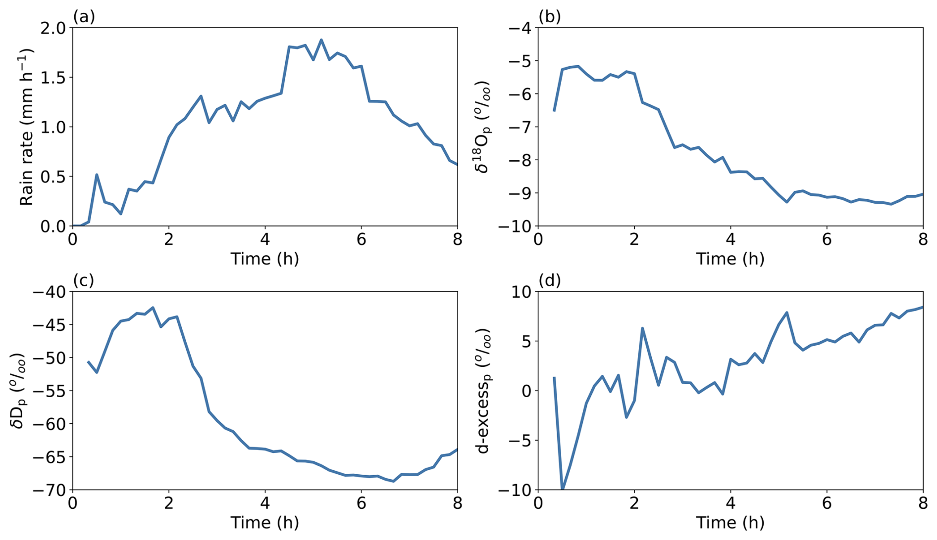
Figure 2 Temporal evolution of (a) the instantaneous surface rain rate (mm h⁻¹), and the isotopic composition of the rain (‰): (b) δ¹⁸O_p, (c) δD_p and (d) d-excess_p. Variables are averaged over the whole domain every 10 min.

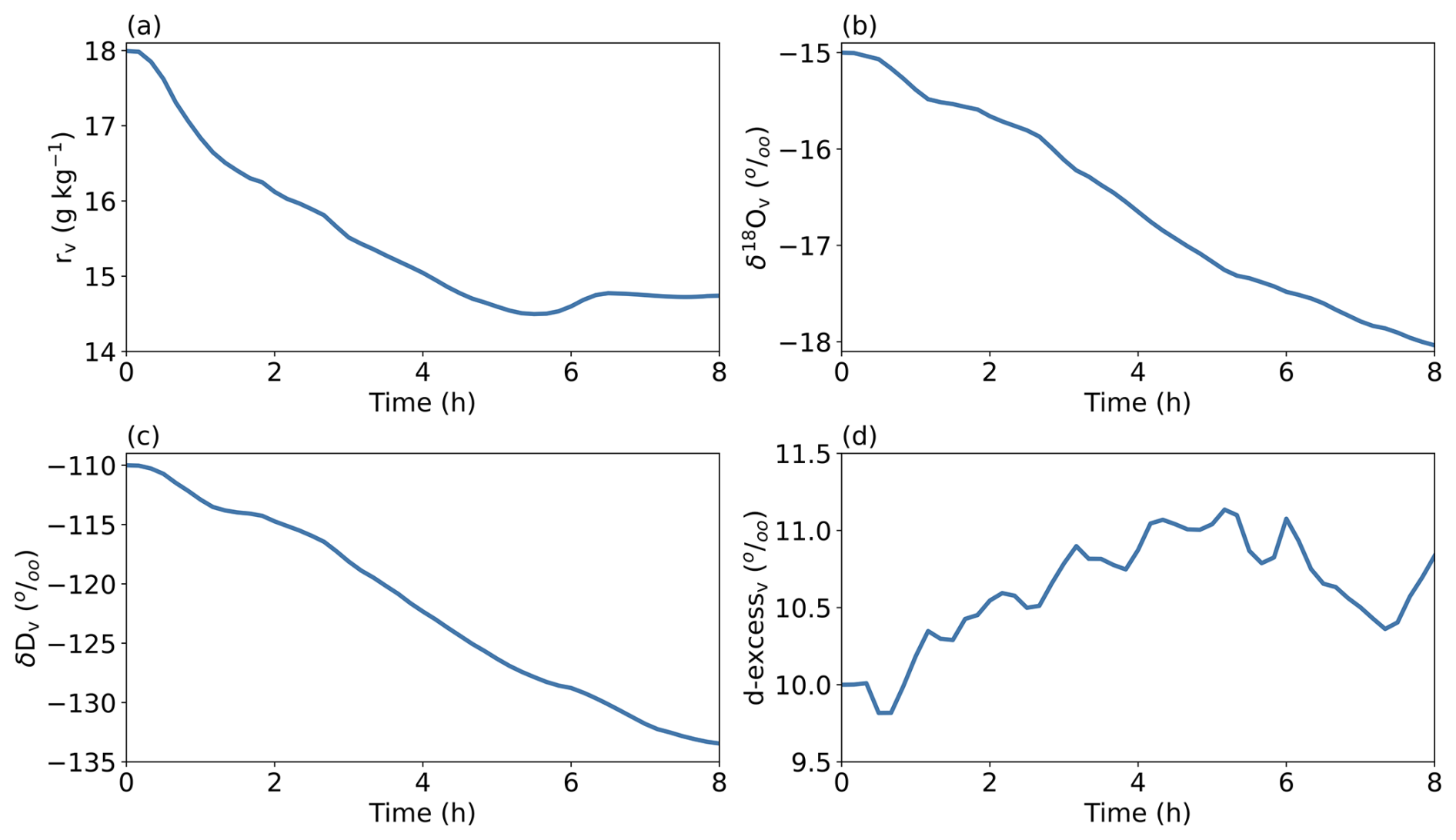
Figure 3 Temporal evolution of (a) the near-surface water vapor mixing ratio (g kg⁻¹), and the isotopic composition of water vapor (‰): (b) δ¹⁸O_v, (c) δD_v and (d) d-excess_v. Variables are averaged over the whole domain every 10 min.

We investigated to understand why the isotopic composition of rain reaches a quasi-steady state in contrast to the isotopic composition of water vapor. During the simulation, convective mixing dries out and depletes the boundary layer (below 1.5 km), and moistens and enriches the free troposphere (Fig. 4a–b). These trends persist throughout the simulation, fading at the end of the simulation as convection weakens significantly after 6–7 h. Water vapor mixing ratio reaches a quasi-steady state at the end of the simulation because the drying effect of convective mixing is offset by the moistening effect of droplet evaporation (Fig. 4c). The isotopic composition of water vapor does not reach equilibrium at the end of the simulation because the depleted effect of convective mixing is reinforced by the depleted effect of droplet evaporation. The isotopic composition of the precipitation appears to reach equilibrium, but this is because two effects compensate each other: (1) the water vapor in the boundary layer, with which the rain equilibrates, is increasingly depleted, so it tends to deplete the rain; (2) the water vapor in the free troposphere, where the droplets form, is more enriched, so it tends to enrich the rain (Fig. 4d).

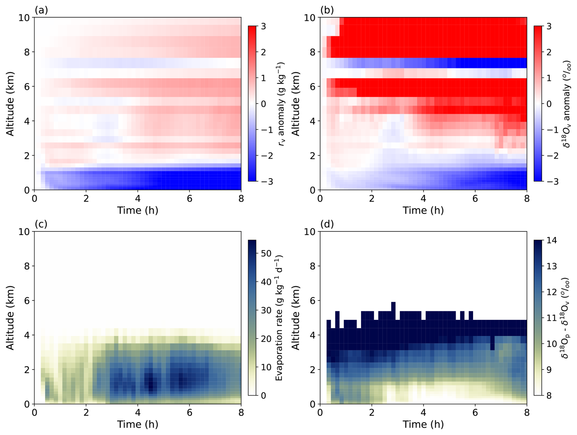
Figure 4 Evolution of some vertical profiles along the course of the simulation: (a) water vapor mixing ratio (r_v, g kg⁻¹) anomaly with respect to the initial vertical profile, (b) isotopic composition of water vapor (δ¹⁸O_v, ‰) anomaly with respect to the initial vertical profile, (c) rain evaporation rate ($\mathrm{g}{\mathrm{kg}}^{-\mathrm{1}}{\mathrm{d}}^{-\mathrm{1}}$), (d) difference between the isotopic composition of rain and that of the water vapor (δ¹⁸O_p−δ¹⁸O_v).

4.4 Structure and dynamics of the squall line

We describe here the structure and the dynamic of the squall line after 6 h of simulation when rain rate is at its highest level and the squall line has reached a mature stage (as already observed in the simulation done by Caniaux et al., 1994). Figure 5 shows the cross section of several parameters sensitive to squall line's structure and dynamic that are shown schematically on Fig. 6 for a better understanding of the description of Fig. 5.

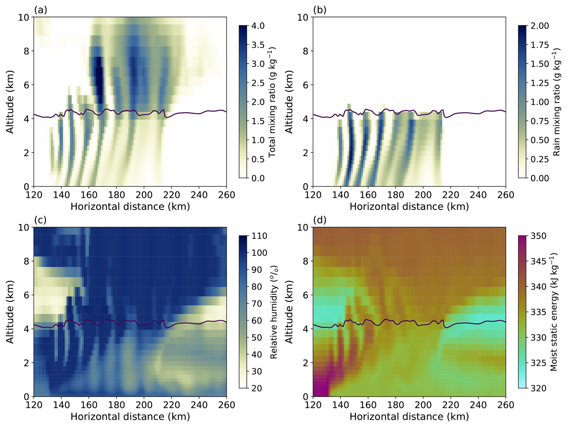
Figure 5 Vertical cross section of the (a) total condensed water mixing ratio (g kg⁻¹), (b) rain mixing ratio (g kg⁻¹), (c) relative humidity (%) and (d) moist static energy (kJ kg⁻¹) after 6 h. The total water condensed mixing ratio is the sum of the mixing ratio of all hydrometeors (cloud droplets, rain, cloud ice, snow/aggregates and graupel). The relative humidity is calculated for saturation over water for temperatures over 0 °C, and for saturation over ice for temperatures below 0 °C. The black line corresponds to the 0 °C isotherm.

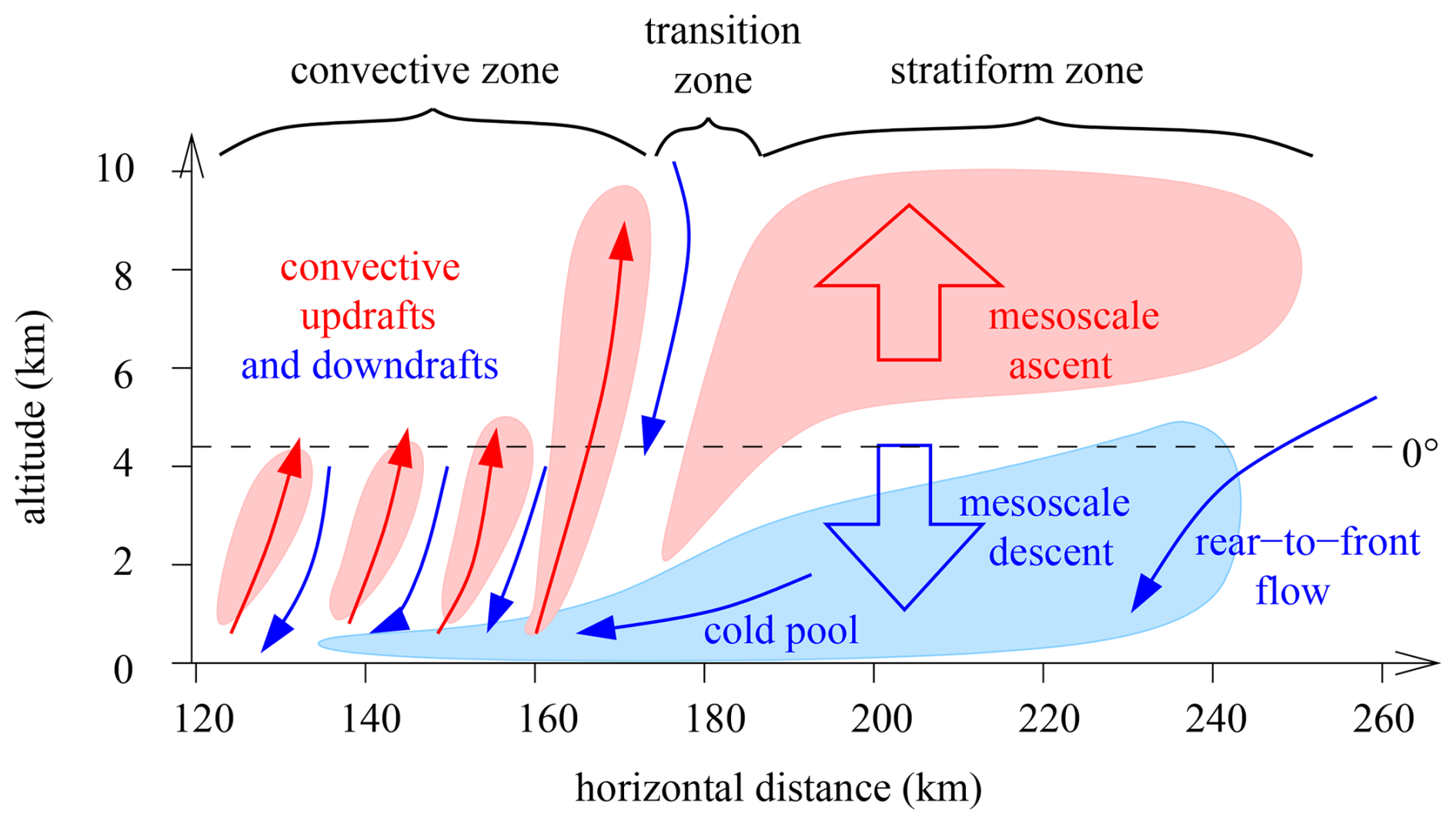
Figure 6 Schematic of the main structural components of a squall line moving from right to left with the three convective, transition and stratiform zones along with horizontal and vertical dynamic.

To visualize the cloud shape, Fig. 5a shows the cross section of the total condensed water (the sum of the mixing ratio of all hydrometeors) along the x-direction. Strong values of condensed water content correspond to strong updrafts. We can see that there is a series of several updrafts from about 135 to 165 km, about 10 km apart from each other, corresponding to various convective cells at different stages, from the shallowest near the front of the squall line (at around 135 km) to the deepest at the rear (at around 165 km). From about 165 to 230 km, most of the condensed water is confined above the melting level, corresponding to the stratiform region, or anvil, of the squall line. This structure is consistent with previous studies (Houze, 1977; Gamache and Houze, 1981; Lafore et al., 1988).

Figure 5b shows the cross section of rain water content. The rain mixing ratio is the strongest below each convective updraft where most of it reaches the ground, whereas below the anvil, most of the rain evaporates before reaching the ground.

Figure 5c and d show the cross section of the relative humidity and the moist static energy, respectively. The high values of relative humidity near or at saturation correspond to the cloud, while lower values correspond to the environment or to subsiding air. The high values of moist static energy correspond to ascending air from the boundary layer to higher altitude, whereas lower values correspond to mid-tropospheric environment or subsiding air. The two snapshots exhibit expected features for well-developed squall lines. We can clearly see the convective region composed of several convective updrafts transporting air from the boundary layer to higher levels from about 135 to 165 km as mentioned above (high relative humidity and moist static energy). We also clearly detect lower relative humidity and moist static energy within downdrafts. The stratiform region is clearly developed. It corresponds to the cloudy area that extends behind the convective zone above around 4 km height from about 195 to 260 km. Below the stratiform region, the cold pool is identified by the dry air with low moist static energy (Fig. 5c and d). It extends frontwards towards the front of the line, around 130 km. Between convective and stratiform zones, the transition region is identified in the simulation by patches of dry subsiding air between around 165 an 195 km and below 4 km height (Fig. 5c).

4.5 Simulated isotopic composition of rain and water vapor after 6 h of simulation

Updrafts in the convective zone are transient, i.e. their exact location varies with time (not shown). Thus, rather than calculating temporal averages when the squall line is most intense, we analyze snapshots at a given time step. In the following, we chose to show results after 6 h of simulation as we can clearly distinguish between the convective and stratiform zones as described in the previous section. We checked that results are qualitatively similar whatever the snapshot we chose during the time interval of 5 to 6 h. Although the stratiform zone is in development earlier in the simulation, we also show isotopic results after 4 h of simulation in the supplementary material to show that (1) the non isotopic steady state has no impact on results and (2) the expected isotopic characteristics are well reproduced elsewhere in the simulation with a squall line at a different stage of development.

To document the isotopic results, we plot two figures. Figure 7a–d shows the cross section of anomalies of the isotopic composition (δ¹⁸O and d-excess) of both water phases. The isotopic anomalies are relative to the domain-mean at each level. In addition, the cross section of the isotopic composition of water vapor and rain are shown in Fig. S1 in the Supplement. We also show on Fig. 7e the difference between the isotopic composition of rain (δ¹⁸O_p) and the isotopic composition of rain in equilibrium with water vapor ((δ¹⁸O_p)_eq deduced from ${\mathit{\alpha }}_{\text{l,v}}=({\mathit{\delta }}^{\mathrm{18}}{\text{O}}_{\text{v}}+\mathrm{1})/\left(\right({\mathit{\delta }}^{\mathrm{18}}{\text{O}}_{\text{p}}{)}_{\text{eq}}+\mathrm{1})$), hereafter named the isotopic disequilibrium for δ¹⁸O (δ¹⁸O_p−(δ¹⁸O_p)_eq). A similar disequilibrium is calculated for d-excess (d-excess_p − (d-excess_p)_eq) and shown on Fig. 7f. The absolute isotopic values are shown on Fig. S1a–d. Figure 8 shows the isotopic composition of both water phases at the surface along the x-direction.

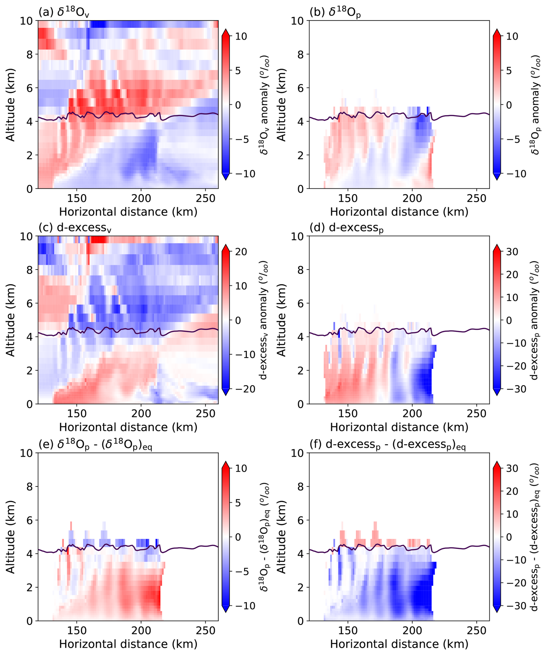
Figure 7 Vertical cross section after 6 h of (a) δ¹⁸O_v, (b) δ¹⁸O_p, (c) d-excess_v, (d) d-excess_p, (e) δ¹⁸O_p − (δ¹⁸O_p)_eq and (f) d-excess_p − (d-excess_p)_eq. Panels (a) to (d) are anomalies calculated by subtracting the average value of the variable at a given altitude from the local value of the variable. The black line corresponds to the 0 °C isotherm. Similar panels with absolute values can be seen on Fig. S1.

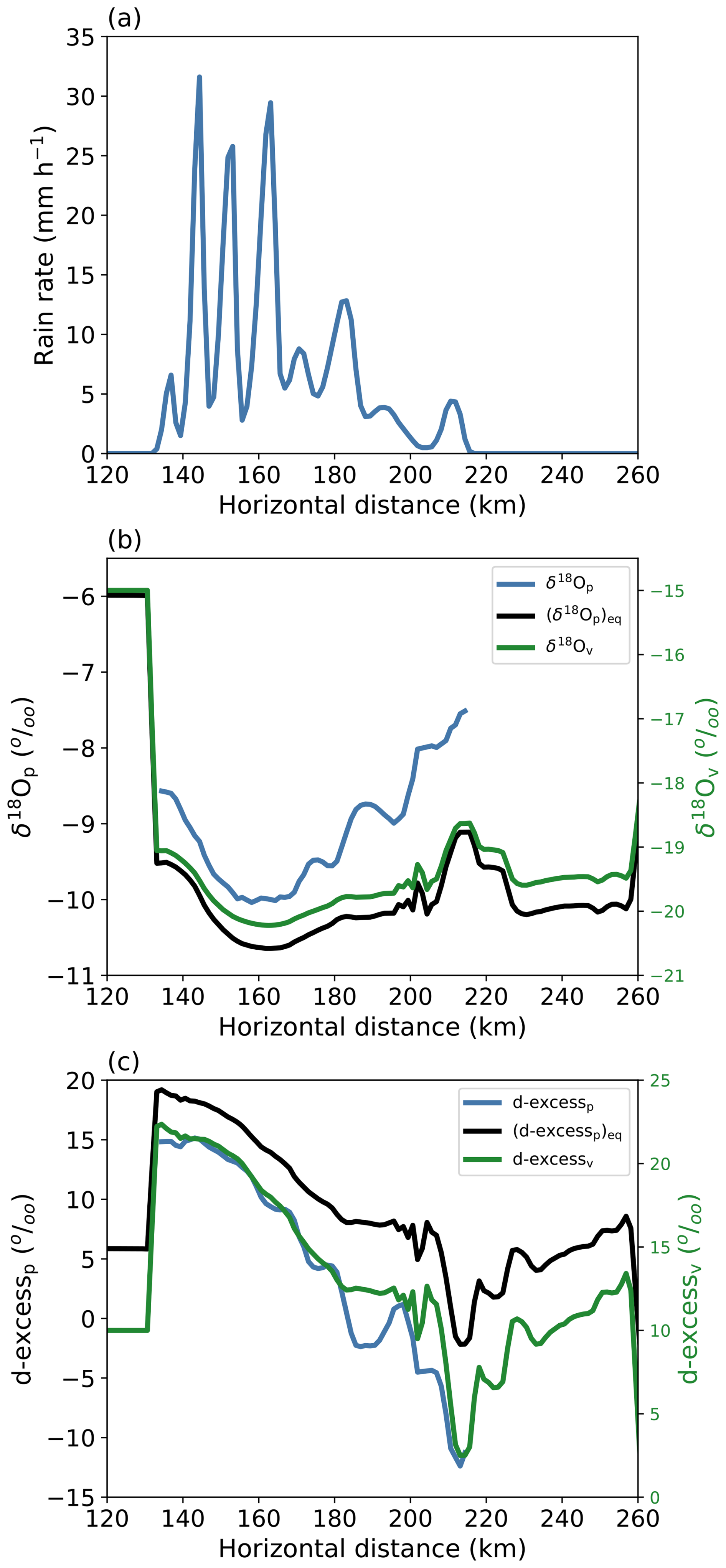
Figure 8 Evolution of the surface rain rate (a), δ¹⁸O (b), and and d-excess (c) along the x-direction after 6 h of simulation. In (b) and (c), the blue, black and green lines correspond to the isotopic composition of rain, rain in isotopic equilibrium with water vapor, and water vapor, respectively. In (b) and (c), the isotopic composition of rain (water vapor) is on the left-y (right-y) axis.

4.5.1 Description of the isotopic variations in the 2D domain

In the convective zone, we clearly distinguish on Fig. 7a the previously identified updrafts with enriched water vapor exported from the surface layer and, in between, downdrafts with lower δ¹⁸O_v reflecting export of depleted water vapor from higher altitude. The narrow vertical plumes of higher δ¹⁸O_p (see Fig. 7b from 1 to 3.5 km) and lower d-excess_p (see Fig. 7d from 1 to 3.5 km) reflect the rain evaporation which preferentially occurs within downdrafts consistent with previous studies (Kurita, 2013; Risi et al., 2021, 2010). The lower d-excess_p when evaporation processes are at play is interpreted as the kinetic effects during rain evaporation. The rain evaporation in narrow downdrafts is also suggested by positive (negative) isotopic disequilibrium for δ¹⁸O_p (d-excess_p) (Fig. 7e–f) (rain evaporation leads rain to be more enriched than expected at isotopic equilibrium and d-excess_p to be lower than expected at isotopic equilibrium, see for example Graf et al., 2019). Both vertical motions and rain evaporation in the convective zone can be seen also in d-excess_v (Fig. 7c). The lower d-excess_v in updrafts suggests the export of low d-excess_v from the surface layer toward higher altitude. The higher d-excess_v in downdrafts is related to rain evaporation (under strong rain, a low fraction of rain evaporation tends to increase d-excess_v) and to air subsidence exporting higher d-excess_v from higher altitude.

In the stratiform zone, under the anvil cloud, the water vapor is more depleted in average than in the convective zone (Fig. 7a) as expected from the progressive depletion of water vapor by rain evaporation, meso-scale downdrafts and higher condensation altitude (Aggarwal et al., 2016; Kurita, 2013; Risi et al., 2021). We can see lower values of δ¹⁸O_p at around 210 km and above 3 km (Fig. 7b). This could reflect that rain originates from snow melt, which is more depleted than the rain that would has formed locally because the snow has formed at higher altitude as already suggested by Risi et al. (2010, 2021) (see also Fig. S2). This is in agreement with the negative disequilibrium for δ¹⁸O_p in this area (Fig. 7e). In contrast, between 200 and 215 km and below 3 km, δ¹⁸O_p is higher and d-excess_p is lower down to the surface (Fig. 7b–d) reflecting the enriched effect of rain evaporation on δ¹⁸O_p and the lowering effect on d-excess_p, consistently with the positive (negative) disequilibrium for δ¹⁸O_p (d-excess_p) in this area (Fig. 7e–f). The impact of rain evaporation is also seen on δ¹⁸O_v in this part of the domain (Fig. 7a) with the expected depleted effect on δ¹⁸O_v. The expected higher d-excess_v is also seen between 200 and 215 km but in a restricted region between 0.5 to 2.5 km height (Fig. 7c).

In the transition zone, the expected isotopic characteristics are more visible on the precipitation phase. We identify in the three dry air patches shown on Fig. 5c (roughly located at 165, 175 and 190 km) both higher values of δ¹⁸O_p and lower values of d-excess_p suggesting that evaporation processes are at play, consistently with strong positive (negative) disequilibrium for δ¹⁸O_p (d-excess_p) (Fig. 7e–f).

Given the major role of evaporation processes in controlling the isotopic composition of both rain and water vapor, we further analyzed theses processes in Sect. 4.5.3.

4.5.2 Description of temporal evolution of the surface isotopic composition

Our simulation exhibits four precipitation maxima in the convective zone corresponding to the aforementioned convective updrafts, followed by lower precipitation in the transition region with two peaks (Fig. 8a). Two precipitation peaks are also seen in the stratiform region: the first one located at 195 km is attributed to stratiform rain as the later falls diagonally toward the front of the system as shown on Fig. 5b. This is consistent with surface observations although usually only one convective precipitation maximum is found (Risi et al., 2010).

Our simulation shows a W-shaped δ¹⁸O_p (Fig. 8b, blue lines). Two local isotopic minima are observed in the convective zone and at the onset of stratiform region at about 160 and 195 km respectively. In the transition region, the peak in the middle of the W is actually formed in our simulation by a double-isotopic peaks (at around 175 and 190 km). This W-shape has often been observed in the isotopic composition of precipitation of squall lines (Rindsberger et al., 1990; Taupin and Gallaire, 1998; Risi et al., 2010). Typically, δ¹⁸O_p in our simulation can be compared to the isotopic variations observed in precipitation collected along the squall line that occurred on 18 August 2006 in Niamey (see Fig. 2 in Risi et al., 2010).

Regarding the simulated δ¹⁸O_v, there is a sharp decrease right after 130 km corresponding to the cold pool front which is observed for more than 85 % of squall lines in Niamey from 2010 to 2012 (Tremoy et al., 2014). Then, δ¹⁸O_v decreases along the convective zone before slightly increasing (about 1 ‰) in the transition and stratiform zones as observed in about 30 % of squall lines in Tremoy et al. (2014).

According to previous studies dealing with conceptual and cloud resolving models (Risi et al., 2021, 2023), the main processes depleting near-surface water vapor in convective and stratiform zones are mesoscale descents, rain evaporation in a moist environment, and enhanced rain-water vapor diffusive exchanges (as rain falls into layers that are more and more enriched, diffusive exchanges tend to enrich the precipitation and deplete water vapor around it). The isotopic decrease in precipitation along the convective zone follows to first order that in the water vapor, both phases being in close equilibrium at the surface (Fig. 8b, black lines).

The decreasing trend in δ¹⁸O_p is however interrupted from the transition zone. Superimposed on the increasing δ¹⁸O_p trend, the two peaks that form the middle of the W reflect the enrichment of rain by evaporation during its fall in dry air (Fig. 5c) as suggested by Risi et al. (2010). Rain is always enriched by evaporation processes but the drier the air, the more enriching evaporation is for a constant fraction of evaporated rain.

The δ¹⁸O_p recovery after 195 km, corresponding to the right limb of the W-shaped pattern, is attributed to increasing evaporative enrichment in the stratiform zone in a drier environment (Risi et al., 2010; Tremoy et al., 2014; Risi et al., 2023) (see also next section).

Deuterium excess in precipitation continuously falls along the simulated squall line and attains strong negative values (−10 ‰) after 210 km during the second precipitation peak in the stratiform zone (Fig. 8c, blue lines) as observed for some squall lines in Risi et al. (2010). This is consistent with rain evaporation aforementioned increasing from the transition zone. We also observe two decreases in d-excess_p in the transition region in phase with the δ¹⁸O_p double peaks consistently with rain evaporation. Deuterium excess in water vapor also decreases along the squall line as observed by Tremoy et al. (2014) for more than 85 % of observed squall lines.

4.5.3 Analysis of the rain evaporation processes

Figure 9a shows the disequilibrium for δ¹⁸O_p at different altitudes (surface, 1 and 4 km). Positive values mean that the rain is more enriched than if it was at equilibrium with water vapor, reflecting evaporative processes. Negative values mean that the rain is more depleted than if it was at equilibrium with water vapor, reflecting rain falling from higher altitude and further depleted.

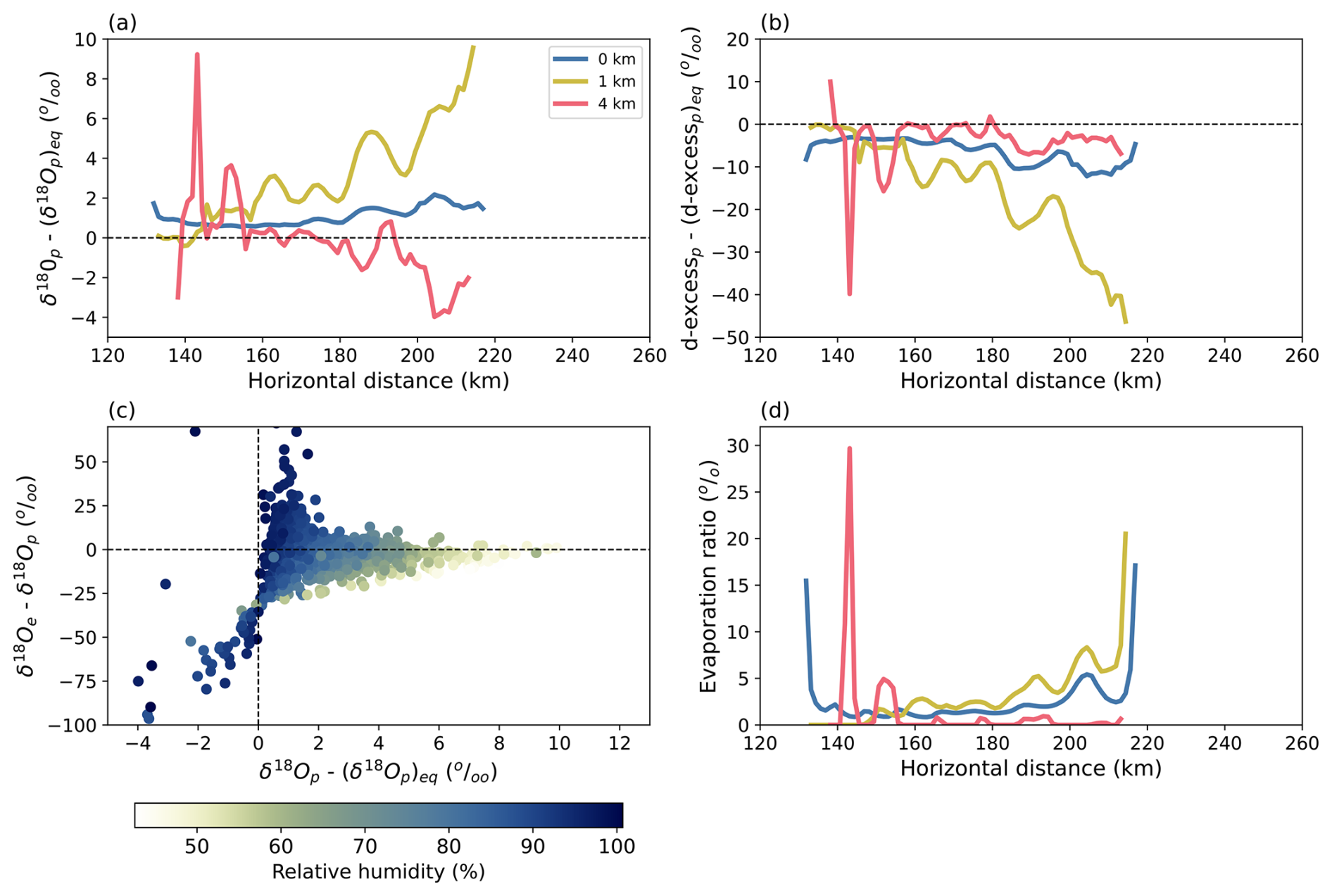
Figure 9 Difference between the isotopic composition of the rain and of the rain at isotopic equilibrium with the vapor at different altitudes for δ¹⁸O (a) and d-excess (b) along the x-direction after 6 h of simulation. (c) Scatter plot of the difference between the δ¹⁸O in the evaporation flux and in the rain (δ¹⁸O_e−δ¹⁸O_p), as a function of the δ¹⁸O in the rain and in the vapor at isotopic equilibrium (δ¹⁸O_p−(δ¹⁸O_p)_eq), for all x-values and altitudes where rain occurs. Markers are colored by relative humidity. (d) Fraction of rain that evaporates along the x-direction after 6 h of simulation at different altitudes. The blue, golden and red lines correspond to the isotopic composition at the surface, 1 km altitude and 4 km altitude, respectively.

At 4 km altitude, rain is more depleted than expected from isotopic equilibrium with water vapor, meaning that it falls from higher altitude (Fig. 9a). This phenomenon increases with the x-direction, reflecting the transition from the convective to the stratiform region, where condensation occurs higher (Fig. 5a). At 1 km, rain is more enriched than expected from equilibrium with water vapor, reflecting evaporative enrichment. This phenomenon increases with x-direction, reflecting the drier and drier air in the mesoscale descent under the anvil. At the surface, the disequilibrium for δ¹⁸O_p is still positive but weaker than at 1 km. The rain is closer to the isotopic equilibrium with the vapor as described in Lee and Fung (2008). The effect of rain evaporation on isotopic results at the surface is also likely reduced because of the presence of a humid surface layer (Fig. 5c). Diffusive exchanges are thus favored instead of rain evaporation leading to first order to isotopic equilibrium between rain and water vapor (Fig. 8, black lines).

The same phenomenon is at play for deuterium excess (Fig. 9b). At 4 km altitude, the rain has a higher d-excess_p than if at equilibrium with water vapor, because the rain falls from higher altitude and d-excess_v typically increases with altitude. At 1 km height, the rain has a smaller d-excess_p due to the impact of rain evaporation that enhances with x-direction. At surface, the disequilibrium for d-excess_p is slightly negative but we can not exclude that the humid surface layer reduces this disequilibrium through diffusive exchanges between both water phases.

The processes controlling the disequilibrium between rain and water vapor are illustrated in Fig. 9c, showing the difference between the δ¹⁸O in the evaporation flux and in the rain (δ¹⁸O_e − δ¹⁸O_p), as a function of the disequilibrium for δ¹⁸O_p for all x-values and altitudes where rain occurs. Where relative humidity is high (dark blue shades), any small disequilibrium between rain and water vapor implies diffusive exchanges between both phases to bring them in equilibrium. For example, if rain is more depleted than expected (negative δ¹⁸O_p−(δ¹⁸O_p)_eq), then δ¹⁸O_e is much more depleted than δ¹⁸O_p to bring rain and water vapor to equilibrium. As a result, rain and water vapor are close to equilibrium (near-zero δ¹⁸O_p−(δ¹⁸O_p)_eq). In contrast, where relative humidity is small (beige shades), the fraction of rain that evaporates is large, and thus the evaporation flux has almost the same δ¹⁸O as rain (near-zero values of δ¹⁸O_e−δ¹⁸O_p). The strong evaporation leads to evaporative enrichment of rain (high values of δ¹⁸O_p−(δ¹⁸O_p)_eq). This behavior is expected, giving us confidence in our implementation of isotopic processes associated with rain evaporation.

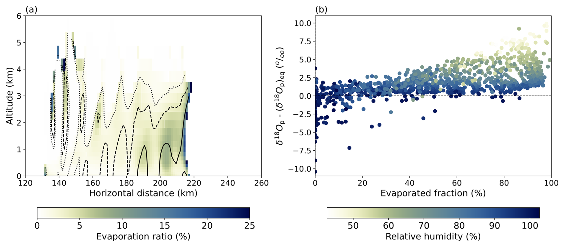
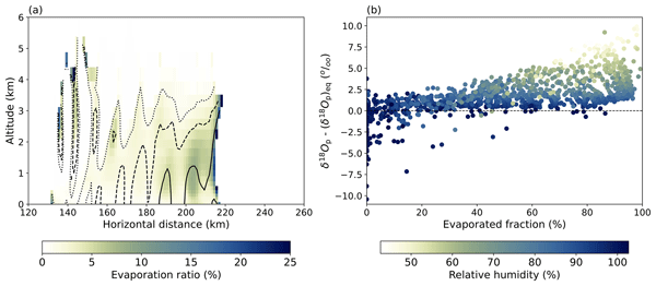
Figure 10 (a) Vertical cross section of the fraction of rain that evaporates (colors; %) after 6 h of simulation. The dotted, dashed and solid lines show respectively the 30 %, 60 % and 90 % isolines of vertically integrated evaporated fraction (f_EVA). The estimate of the vertically integrated evaporated fraction assumes a drop fall velocity of 5.6 m s⁻¹. Similar results are obtained for a lower (2.8 m s⁻¹) and a higher (11.2 m s⁻¹) drop fall velocity. (b) Scatter plot of the isotopic disequilibrium (δ¹⁸O_p−(δ¹⁸O_p)_eq) as a function of the vertically integrated evaporated fraction (f_EVA), for all x-values and altitudes where rain occurs. Markers are colored by relative humidity (%).

As a first exploration, we defined an estimate of the evaporated fraction of rain in the model. We show on Figs. 9d and 10a the ratio between the tendency of rain evaporation (evaporation flux derivative as a function of time) and the mixing ratio of rain. This ratio is the rain-normalized evaporated fraction of rain in each grid (0 % means that no evaporation occurred, 100 % means that all rain evaporated):

$$\begin{array}{}\text{(34)}& R_{\text{EVA}}={\displaystyle \frac{\mathrm{\Delta }r{|}_{\text{EVA}}\times \mathrm{\Delta }t}{r_{\text{r}}}}\times \mathrm{100}\end{array}$$

with Δt the model time step.

We also calculated at each level z the fraction of the rain that has evaporated during its fall since it was produced, f_EVA, as the ratio between the rain evaporation flux to the rain flux if the evaporation was absent (Fig. 10):

$$\begin{array}{}\text{(35)}& f_{\text{EVA}}\left(z\right)={\displaystyle \frac{E\left(z\right)}{P\left(z\right)+E\left(z\right)}}\end{array}$$

where P(z) is the rain flux at level z and E(z) is the rain evaporation flux between level z and the top of the domain. P(z) is calculated as $P\left(z\right)=r_{\mathrm{r}}\times {\mathit{\rho }}_{\text{a}}\left(z\right)\times V_{\mathrm{t}}$ where r_r is the rain mixing ratio and V_t is a terminal velocity taken as 5.6 m s⁻¹. E(z) is calculated as:

$$\begin{array}{}\text{(36)}& E\left(z\right)=\underset{z^{\prime }=z}{\overset{z_{\mathrm{top}}}{\int }}\mathrm{\Delta }r{|}_{\text{EVA}}\left(z^{\prime }\right)\times {\mathit{\rho }}_{\text{a}}\left(z^{\prime }\right)\times \mathrm{d}{z}^{\prime }\end{array}$$

In the convective zone, evaporation occurs in the narrow dry downdrafts between 2 and 4.5 km height and evaporation rate can attain up to around 25 % in a few grids (Figs. 9d and 10a). In the transition zone, rain evaporation is present within the dry patches of subsiding air from about 0.5 to 3.5 km with an evaporation rate varying between 0 % and 10 % at a given level. At last, Figs. 9d and 10a clearly show that rain evaporation is present almost all over the domain under the anvil cloud and reaches a maximum at the edge of the stratiform zone (at about 215 km) where evaporation rate attains close to 25 % all along the vertical dimension from the near-surface to 3.5 km height. The vertically integrated evaporated fraction of rain reaches a maximum (higher than 60 %) in the convective zone in downdrafts where relative humidity is lower and below the stratiform zone with values higher than 90 % (Fig. 10a). The expected influence of evaporative effects on the isotopic composition of precipitation is clearly captured by our simulation as shown on Fig. 10b. The isotopic disequilibrium (δ¹⁸O_p−(δ¹⁸O_p)_eq) increases with positive values as the vertically integrated evaporated fraction increases and the relative humidity decreases.

This 2D spatial pattern of the rain evaporation is consistent with the spatial isotopic variations of water vapor and precipitation, giving us confidence again in our implementation of isotopic processes associated with rain evaporation. Our estimate for the vertically integrated evaporated fraction of rain can be compared to previously published values. Based on a box model aiming at reproducing the near-surface observations, Tremoy et al. (2014) concluded that for a majority of squall lines, the rain evaporation rate varies between 10 % and 35 % with a maximum at the rear of the stratiform zone that can attain almost 60 % in a few cases. Using cloud resolving model in radiative-convective equilibrium to simulate an idealized squall line, Risi et al. (2023) simulated a similar range for the rain evaporation rate in the convective and stratiform zones, increasing up to 90 % in the trailing environment as also obtained in our simulation below the stratiform cloud.

5 Conclusions

This paper presents the implementation of water stable isotopologues in the non-hydrostatic mesoscale model Meso-NH. This development is tested with the simulation of a squall line that occurred at night on 23–24 June 1981 during the COPT 81 intensive field campaign. We chose this squall line as it was subject to comprehensive observations on the field and as a 2D simulation was done by Caniaux et al. (1994) with Meso-NH. Our simulation successfully reproduces the main expected spatial structure of a mature and intense squall line after 6 h of simulation: a convective zone, a transition zone and a stratiform zone where different processes are expected to produce different isotopic fractionation on water vapor and precipitation.

It is worth noting that even though the isotopic composition of near-surface vapor isotopes continues to evolve late in the simulation, while water vapor amounts and isotopic composition of precipitation isotopes settle into a quasi-steady-state, the results are actually consistent with observations after 6 h. This is also true earlier in the simulation as shown for example after 4 h of simulation when the convective zone is formed and the stratiform region is developing (Figs. S3 to S7). This result suggests that the non-isotopic steady state in near-surface water vapor at the end of the simulation does not prevent us from exploring the isotopic variations of water in our simulation.

The Meso-NH-ISO model captures well the main isotopic features expected as seen in many observations:

• Regarding the spatial pattern of the isotopic composition of water in the 2D domain: (i) In the convective zone, our simulation well reproduces the enriched and depleted water vapor in updrafts and downdrafts respectively reflecting both vertical motions of water and rain evaporation processes. (ii) In the transition zone, the impact of rain evaporation processes on the isotopic composition of precipitation is also well reproduced in the dry plumes of subsiding air with an enrichment of δ¹⁸O_p, low – even negative – values of d-excess_p and a positive disequilibrium for δ¹⁸O_p. (iii) In the stratiform zone, our simulation captures the expected processes. The low δ¹⁸O_p in altitude reflects the higher altitude of condensation in this zone. The negative values of d-excess_p and the highest values of δ¹⁸O_p below the anvil cloud reflect rain evaporation processes, specifically at the rear of the stratiform zone where our estimate of the fraction of rain that evaporates is the stronger. Indeed, the fraction of the rain that has evaporated during its fall can be higher than 90 %. The analysis of evaporation processes in our simulation shows that these processes act as expected in modulating the isotopic composition of water in the 2D domain.

• Regarding the comparison with the observations of the isotopic composition of water at the surface: (i) Along the squall line, δ¹⁸O_p evolves along a W-shaped pattern as observed for numerous squall lines by Rindsberger et al. (1990), Taupin and Gallaire (1998), and Risi et al. (2010). The increasing δ¹⁸O_p in the middle of the W and at the end of the W, attributed in previous studies to rain evaporation in a drier environment in the transition zone and at the rear of the stratiform zone, are well reproduced in our simulation. (ii) δ¹⁸O_v decreases along the convective zone before slightly increasing in the transition and stratiform zones as observed in about 30 % of squall lines in Tremoy et al. (2014). The lowering of δ¹⁸O_v has been explained in previous studies as reflecting mesoscale descents, rain evaporation and favored diffusive exchange between rain and water vapor in moist environment. (iii) Deuterium excess in precipitation and water vapor decreases along the squall line as already observed in Risi et al. (2010) and Tremoy et al. (2014) respectively that is consistent with rain evaporation, mesoscale descents and presence of a enhanced diffusive exchanges at surface.

The plans for this implementation is to use Meso-NH-ISO for realistic cases of squall lines and cyclones in order to better understand what are the controls on the isotopic composition of water in convective systems. For example, Vimeux et al. (2024) recently showed the presence of a very organized signal in the isotopic composition of water vapor within cyclones on an hourly scale, empirically linked to the spatial structure of cyclones. Observations alone and general atmospheric climate models, even with a high spatial resolution, have not been able to decipher the processes controlling isotopic variations in water vapor and therefore to quantify them. Future simulations with Meso-NH-ISO should enable further advances on this aspect with the final objective of better studying and quantifying convective processes from water stable isotopologues. Furthermore, Meso-NH now features a two-moment mixed-phase microphysical scheme (LIMA, Vié et al., 2016; Taufour et al., 2024) which does not assume a saturation adjustment for ice. Plans are in place to integrate the stable water isotopologue scheme with LIMA in the near future, in order to benefit from the advantages of a two-moment microphysical scheme and to better account for the fractionation of heavy isotopologues during both the liquid-vapor and vapor-ice transitions.

Appendix A

Table A1 List of symbols.